Opportunities for and Impacts of Carsharing: A Survey of the Austin, Texas Market

By

Bin (Brenda) Zhou

Graduate Student Researcher The University of Texas at Austin

6.508. Cockrell Jr. Hall Austin, TX 78712-1076

brendazhou@mail.utexas.edu

Kara M. Kockelman (Corresponding author)

Associate Professor and William J. Murray Jr. Fellow Department of Civil, Architectural and Environmental Engineering

The University of Texas at Austin 6.9 E. Cockrell Jr. Hall Austin, TX 78712-1076

kkockelm@mail.utexas.edu Phone: 512-471-0210 FAX: 512-475-8744

The following paper is a pre-print and the final publication can be found in the

International Journal of Sustainable Transportation 5 (3): 135-152, 2011. Presented at the 87th Annual Meeting of the Transportation Research Board, January 2008.

ABSTRACT:

Carsharing involves the communal ownership and use of a fleet of vehicles, typically on an hourly basis (Millard-Ball et al. 2005). Austin CarShare (ACS) was launched in the fall of 2006, making Austin the first city in Texas with carsharing services. While many studies have discussed the positive impacts of carsharing, few have examined widespread public opinion of carsharing. This study undertook the challenge of investigating traveler preferences during ACS’s service launch, in order to anticipate latent demand for such services.

The survey provides rich information on public opinion of different aspects of the ACS program, as well as the expected demand on the service and possible changes in travel patterns. Supplementing the survey results with spatial data, membership models of two pricing plans reveal that households with higher vehicle ownership and income-to-adults ratios are less likely to join the program, while level of education exhibits a convex relationship with the probability of joining the Freedom Plan, ceteris paribus. Although potential carsharing users share similar characteristics, the two plans serve slightly different customer sets and have the potential to supplement one another.

1. INTRODUCTION Automobile use is the source of many current woes, including air pollution (Kearney and

De Young 1996), greenhouse gas emissions (Walsh 1993), loss of life and property (Evans 2004), and, of course, traffic congestion (Schrank and Lomax 2005). Carsharing is an innovative approach to reducing the negative impacts of private vehicle ownership, while providing a relatively low-cost and flexible transportation alternative.

As indicated by its name, carsharing provides an individual or business access to a fleet of shared-use vehicles on demand. It distinguishes access from ownership such that program members reap the benefits of private vehicle access without the onus of ownership. Members pay a fee each time they use a vehicle, based on mileage traveled and/or travel duration. Other types of fees also exist in many carsharing programs, including security deposits, one-time membership fees, and annual or monthly fees.

Carsharing began in Switzerland in 1948, and became popular in the early 1990’s (Shaheen and Cohen 2006). European evidence indicates that carsharing members drive less than they did before becoming members, and some sell one or more of their personal vehicles after joining (Steininger et al. 1996; Meijkamp 1998; Koch 2001). The United States’ first commercial carsharing organization was Car Sharing Portland, in the state of Oregon (Katzev 2003). Established in 1998, it was preceded by two demonstration programs: Mobility Enterprise (a research program launched by Purdue University in Indiana) and San Francisco’s Short-Term Auto Rental (STAR) program (Shaheen et al. 1998). U.S. carsharing membership experienced exponential growth between 1998 and 2004 (quadrupling membership levels each year, on average), with something of a slow down during 2005 (with only 46% more members added that year) (Shaheen et al. 2006). According to Shaheen’s (2007) recent count, there are 18 carsharing organizations in the U.S., with 134,094 members for about 3,637 vehicles.

Carsharing is gaining popularity worldwide, but U.S. public opinion remains unclear, particularly in regions without pedestrian friendly and transit ready environments. In addition, while several studies have suggested that carsharing reduces congestion, improves air quality, and enhances regional accessibility for non-auto-owning populations while increasing transit share and reducing reliance on the private automobile (see, e.g., Steininger et al. 1996; Rodier and Shaheen 2004; and Shaheen and Rodier 2005)1, less attention has been paid to the anticipated demand for such programs and associated factors. To address these issues, this study investigates Austinites’ preferences for such services using a self-complete survey that took advantage of several distribution channels. Multivariate models of choice behavior help disentangle various demographic, location and other factors’ effects on program participation.

The following sections discuss survey implementation and the collected data, as well as the results of models of plan membership.

2. SURVEY DESIGN AND DISTRIBUTION Since ACS was being launched at the time of the survey, almost no respondents had prior

experience with carsharing. The stated response data used here cannot guarantee that the respondents will actually behave as they stated. Nevertheless, the objective of understanding

1 While environmental and economic benefits are commonly associated with carsharing programs, behavioral results can and do vary over time. For example, Cervero (2003) noted that in the first year of joining City CarShare, members tended to increased their VMTs relative to a “control group” (of persons who had indicated an interest in joining but had not yet joined) because of their new access to carsharing vehicles; however, the second-year study found an overall decline in VMT by members (Cervero and Tsai 2004).

public opinion of carsharing before actually experiencing the service is reasonable. At the time of the survey, many Austinites had been exposed to the concepts, operations, and expected benefits of ACS via local media. In addition, a color brochure from ACS was distributed together with a paper survey and internet survey respondents were provided links to the ACS website http://www.austincarshare.org/, helping respondents understand the nature of Austin’s carsharing program.

The survey consists of five sections, requesting demographic information, current travel patterns, attitudes toward program attributes, expected changes in travel patterns (when participating in the ACS program) and attitudes toward various program scenarios. Pilot survey feedback and solicitation of expert reviews enhanced instrument design. The final questionnaire totaled eight pages (as shown at http://utwired.engr.utexas.edu/trafficSurvey/) and required approximately 20 minutes to complete.

The survey was developed in both hard-copy and online formats, and was distributed door-to-door in various neighborhoods, as well as by advertising the questionnaire’s URL via card distribution and posted fliers. The survey’s URL also was advertised by hyperlinks shown in the homepages and emails of several neighborhood associations, Austin CarShare (http://www.austincarshare.org/), the Capital Area Metropolitan Planning Organization (CAMPO), UT student organizations, and UT’s division of parking and transportation.

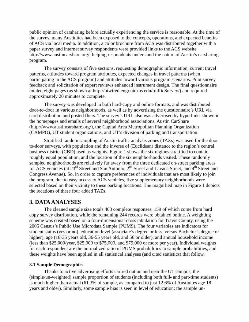
Stratified random sampling of Austin traffic analysis zones (TAZs) was used for the door-to-door surveys, with population and the inverse of (Euclidean) distance to the region’s central business district (CBD) used as weights. Figure 1 shows the six regions stratified to contain roughly equal population, and the location of the six neighborhoods visited. These randomly sampled neighborhoods are relatively far away from the three dedicated on-street parking areas for ACS vehicles (at 23rd Street and San Antonio, 2nd Street and Lavaca Street, and 4th Street and Congress Avenue). So, in order to capture preferences of individuals that are most likely to join the program, due to easy access to ACS vehicles, five supplementary neighborhoods were selected based on their vicinity to these parking locations. The magnified map in Figure 1 depicts the locations of these four added TAZs.

3. DATA ANALYSES The cleaned sample size totals 403 complete responses, 159 of which come from hard

copy survey distribution, while the remaining 244 records were obtained online. A weighting scheme was created based on a four-dimensional cross tabulation for Travis County, using the 2005 Census’s Public Use Microdata Sample (PUMS). The four variables are indicators for student status (yes or no), education level (associate’s degree or less, versus Bachelor’s degree or higher), age (18-35 years old, 36-55 years old, and 56 or older), and annual household income (less than $25,000/year, $25,000 to $75,000, and $75,000 or more per year). Individual weights for each respondent are the normalized ratio of PUMS probabilities to sample probabilities, and these weights have been applied in all statistical analyses (and cited statistics) that follow.

3.1 Sample Demographics

Thanks to active advertising efforts carried out on and near the UT campus, the (simple/un-weighted) sample proportion of students (including both full- and part-time students) is much higher than actual (61.3% of sample, as compared to just 12.6% of Austinites age 18 years and older). Similarly, some sample bias is seen in level of education: the sample un-

weighted average education level is 3.48 (on a five-point scale2), while it is only 3.11 for the general, adult population. And, as one might expect, sample age and income levels are lower than Austin averages: sample age averages 2.32 on a six-point scale3, as compared to 3.13 (among Austin’s adult population); and annual household income averages 3.49 (versus 4.04) on an eight-point scale4.

The other three demographic variables (gender, household size and household vehicle ownership) have relatively little bias: 52.9% versus 51.2% males, 2.80 versus 2.83 persons (on a six-point scale, capped at 6+ persons per household), and 1.77 versus 1.89 vehicles (on a six-point scale capped at 6 vehicles per household). Therefore, only student status, education level, age and household income were used to develop and assign respondent weights, to much better reflect the true Austin or Travis County population. Table 1 offers summary statistics for all sample variables (both before and after weighting). Once the distributions of these four demographic variables were controlled for (by weighting the sample according to PUMS), the corrected sample characteristics mirror the population. The following analyses and statistics in this section are all based on the demographically weighted sample’s distribution.

3.2 Current Travel Patterns

Current travel needs are a key component in assessing potential demand for carsharing vehicles. Austin does not have many mixed use neighborhoods or substantial public transit infrastructure, and driving alone dominates mode choice for five of the six trip purposes: work (71.1% of the weighted sample), food shopping (78.6%), non-food shopping (75.3%), errands/personal activities (76.0%) and social activities (57.5%). Only in the case of school travel (by college students, ages 18 and up) did other modes actively compete: 47% of students listed driving alone as their most common mode, followed by bus (25.4%) and walking (13.6%).

The great majority (80%) of respondents report spending less than 30 minutes traveling from home (one-way) for six trip purposes. Food shopping trips tend to be shorter in duration (just 5.4% over 30 minutes, and 25.1% reporting travel times of 5 minutes).Roughly half the corrected sample reports spending $250 to $499 for car insurance and $50 to $199 for maintenance (for their primary vehicle) every six months. About One-third (32.9%) reports spending $50 to $99 per month on gasoline for their primary vehicle, and nearly one-third (31.2%) spends $100 to $200 per month. The great majority of respondents (84.4%) spend less than $25 (the lowest category listed in the survey) on parking each month. It seems parking expenditures are relatively modest among all car-related expenditures. Even though few Austinites pay for parking, ACS provides free parking in metered spaces and high-density locations, as an incentive to join the program.

While similar fractions of respondents report making 3 or fewer trips on a normal

2 The five education levels are as follows: 1 = less than high school, 2 = high school diploma or equivalent, 3= Associate’s or technical degree, 4 = Bachelor’s degree, and 5 = Master’s degree or higher. While the PUMS data offer these five categories, only a two-level indicator variable was used to weight the data records in the multivariate regression analyses, since bins would have been too small (have too few observations) if all five education levels had been used. 3 The six age categories are as follows: 1 = 18-20 years old, 2 = 21-35 years old, 3 = 36-45 years old, 4 = 46-55 years old, 5 = 56-65 years old, and 6 = 66 or older. 4 The eight income categories are as follows: 1 = less than $15,000 per year, 2 = $15,000 to $24,999, 3 = $25,000 to $49,999, 4 = $50,000 to $74,999, 5 = $75,000 to $99,999, 6 = $100,000 to $149,999, 7 = $150,000 to $199,999, and 8 = $200,000 or more.

weekday (specified as “last Thursday” in the questionnaire) as on a normal Saturday (67.8% vs. 70.0%), a fair number (14.2%) report making 6 or more trips on Saturdays, as opposed to weekdays (6.2%, when time is more constrained). This statistic suggests that carsharing demand is likely to peak on the weekends, when many (relatively short) activities are pursued.

Only 24.1% of the population-weighted respondents report being somewhat or very dissatisfied with their current travel patterns. While many people may not find current surface transportation conditions (including congestion levels) in Austin to be “satisfactory”, they do appear to be largely satisfied with and/or accustomed to their current travel patterns, including modes chosen and expenditure levels. Nevertheless, 24.1% is significant in terms of a potential base of members for the ACS program. System attributes or conditions that respondents most wish to change are travel times (too long), travel costs (too high) and inconveniences in car maintenance. These concerns relate nicely to the benefits of a carsharing program. An ACS membership may dramatically reduce travel costs for car-owning members (by allowing sale of one’s vehicle or other mode shifts), while “freeing” members from the burden of car maintenance. In addition, ACS has the potential to reduce its members’ mileage demands (by incentivizing greater use of bus and non-motorized modes, as well as closer destination choices and fewer “un-planned” trips), thereby alleviating traffic congestion and reducing system travel times.

3.3 Opinions on Program Attributes

Initially, ACS had only three dedicated on-street parking locations5 (two in downtown and one in “West Campus”, near the University of Texas). The survey reveals that less than 30% of the corrected-sample’s respondents are willing to walk more than a half mile to their reserved car, and less than half are willing to spend more than 5 minutes on a bus in order to reach the dedicated parking locations. Obviously, vehicle accessibility can be critical to the program’s success.

ACS is currently offering two pricing plans, as specified in Table 2. The survey results suggest that Freedom Plan is slightly preferred to the scaled-back Limited Plan. Since access to ACS vehicles positively influences one’s stated willingness to join ACS and several sample neighborhoods were selected based on their vicinity to the dedicated parking locations, access to ACS vehicles is included in the weighting scheme, in order to correct for or counter-balance such sample biases. The probabilities of joining the two pricing plans for the demographically and spatially weighted sample, together with the weighting scheme, are discussed in detail in the following section, related to program participation.

Keeping their current travel expenses in mind, more than half of the (corrected) sample perceives the hourly and per-mile rates for both plans to be “too high” or “far too high”. Most ranked scheduling reliability, overall convenience and program cost as the most important factors in making the decision to join (or not join) ACS. In contrast, environmental considerations, condition and type of vehicles, and current gasoline price are not key factors. Moreover, even though the U.S. has experienced dramatic increases in gasoline prices in recent years (Bomberg and Kockelman, 2007), current gas prices do not appear to be important factors in most respondents’ decision-making. The rather high cost of vehicle use under both plans (at 44¢/mile – as compared to fuel costs of roughly 15¢/mile, assuming a 20 mile/gallon vehicle and $3/gallon 5 Currently, ACS has four parking locations, with the newest on the north side of the UT campus, in an area called Hyde Park.

gas price) may contribute to this insensitivity.

In terms of the greatest obstacle to joining the ACS program, 38.0% suggest that they can not join because they need a car too often. And 15.3% state that the program is too costly. Of course, this perception varies quite a bit, by location, culture, and demographic. For example, the high cost of car ownership is the primary reason given by those joining Leiden’s car-sharing program in the Netherlands (Meijkamp 1998), and expected financial saving is listed as the second most important reason for joining Car Sharing Portland (Katzev 2003). While many Austinites may not fully appreciate the potential financial advantages of car-sharing, most of those who end up joining certainly would.

3.4 Expected Change in Travel Behavior

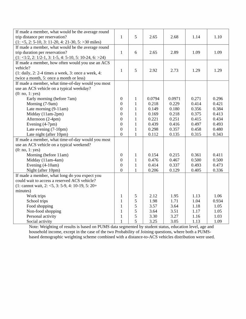
The survey also examined how respondents expect to behave if made a member of the ACS program and if a carsharing vehicle were available “near” their home6. Under these strong assumptions, 21.2% of the population-weighted sample expects to sell at least one of their private vehicles eventually. This is consistent with findings in Meijkamp (1998), Cervero and Tsai (2004) and Shaheen and Rodier (2005). In terms of anticipated demands on ACS vehicles, 31.3% expect to drive just 5 to10 miles in a round-trip reservation, and 38.5% expect to drive between 1 and 5 hours per reservation. In addition, 35.7% expect to make a reservation just once a week – or less often. Of course, use frequency may be very difficult for most respondents to judge, especially before actually experiencing ACS services, and 30.5% simply chose the “Do not know” option7. On a normal weekday, the most popular time for using carsharing appears to be the early evening (4 to 7pm). In contrast, stated weekend demand is found to peak mid-day (11am to 4pm).

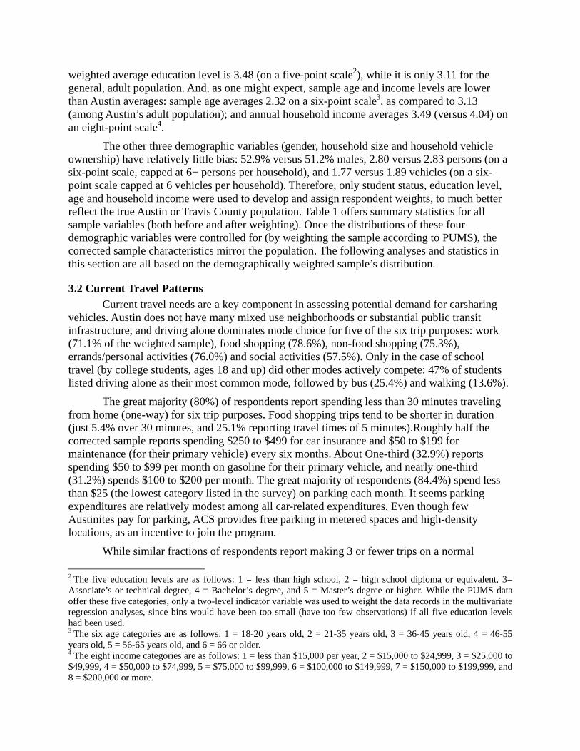
Not surprisingly, people are less willing to wait to access reserved cars (if the scheduled car were delayed) for work/school trips, relative to other trip types. Figure 2 shows the shifts in acceptable wait times across trip purposes. Ideally, ACS might choose to track trip purpose with each reservation and ensure that business-related trips have highest priority if supply falls short.

Austinites are generally hesitant to rely much on ACS vehicles. About half suggested they expected to make 1 or fewer trips per week using ACS vehicles for any of the six trip purposes (after, hypothetically becoming a member). In addition to the public’s general unfamiliarity with such innovative programs, Austin’s limited public transit system, and relatively low intensity development patterns (average density of Travis County is 1.37 persons per acre) contribute to the relative low use of carsharing service across the city’s general population.

4. Program Participation As discussed above, proximity to ACS vehicles will influence one’s decision to join the

program, and five neighborhoods near ACS vehicle parking locations were deliberately chosen for door-to-door survey distribution. Therefore, in addition to the four demographic attributes controlled for in the previous section, distance to the service area was added to the weighting scheme when analyzing the likelihood of program participation/ACS membership.

6 “Near” is defined to mean within 20 minutes by walking, 10 minutes by bus – not including waiting time, and 5 minutes by car – if someone is able to drive the respondent to the reserved vehicles 7 While most questions in this section of the survey offered a “Do not know” option, the reservation frequency question exhibited the highest proportion of respondents choosing this option.

CAMPO’s population counts at the TAZ level were stratified into six categories based on an average of Euclidean distances (for all zone pixels [each measuring 60 ft x 60 ft]) to the nearest dedicated on-street parking space for an ACS vehicle. The number of Austinites residing within 0.5 mile, 0.5 to 1 mile, 1 to 2 miles, 2 to 5 miles, 5 to 10 miles, and over 10 miles to the nearest parking location provide the population proportions here. The numbers of respondents whose homes are located in these six spatial strata in the demographically weighted sample were weighted as the normalized ratio of population probabilities to sample probabilities. This spatial weight was later multiplied by the demographic (non-spatial) weight for each respondent, and these compound weights have been applied in the program participation projection and associated regression models, described below8.

Distributions of (ordered) responses to questions about respondents’ likelihood of joining the two pricing plans vary noticeably when results are weighted. Table 3 shows the results from the unweighted/original sample, the demographically weighted sample, and the compound weighted (both demographically and spatially) sample, indicating that the demographically weighted data over-estimate favorable/high-likelihood-of-joining responses (including “definitely” will join, “very likely”, “probably” and “decent chance” of joining). Such results underscore the fact that demographic unbiasing is inadequate in cases where proximity and/or other spatial effects are at play.

Population-corrected responses to the likelihood-of-joining questions provide some sense of membership potential for the ACS program. Since ACS requires members be at least 21 years of age, have a valid driver’s license, at least two years driving experience, and a good driving record9, one might assume that 70% of Travis County’s age 21+ population (or roughly 430,000 persons) qualifies for membership. In this fashion, the sample-corrected stated probabilities suggest that 6,333 Austinites could be expected to “definitely join” the Freedom Plan, but just 64 for the Limited Plan10. If probabilities for the other response categories are assumed to be 0.8 (“very likely” will join), 0.5 (probably), 0.3 (decent chance), 0.2 (maybe), 0.05 (probably not) and 0.0 (definitely not), the expected number of joiners is a whopping 57,500 Travis County residents (or 13.4% of the assumed-to-qualify population) will join the Freedom Plan and a staggering 45,850 (10.7% of the total qualified population) could be expected to join the Limited Plan.

Of course, these high numbers are highly unlikely, given that San Francisco’s popular City CarShare program presently has just 5,169 members while the city itself has at least 350,000 qualified adults (Nesbitt 2007). Nevertheless, a recent Swedish study (Vägverket, 2003) also found a high stated probability of joining: 25% of respondents stated a willingness to join such a carsharing program11, yet only 0.08% currently are members (Schillander, 2007). Such exaggeration of willingness to join carshaing coincides with the regular bias in goods valuation

8 Compound weights were not used in the earlier analyses, of sample responses simply because those other questions are not clearly related to the actual locations of the vehicles. In fact, several are hypothetical in nature, and assume vehicles are near the respondent. 9 Austin CarShare (2007) defines a good driving record as “no more than one moving violation or accident in the last 18 months, no more than 2 violations or accidents in the last 3 years, and no DWI/DUIs in the last seven years”. 10 The questionnaire asked the probability of joining the two pricing plans within the next six months, but such forecasts may be more likely to represent the total, long-term potential market in Austin, if ACS vehicles remain in their current locations (west of the UT campus and downtown). 11 Among the 25%, 6% said they were definite about this and the rest 19% responded that their decisions were probable.

studies when using stated preference surveys. Many studies find that respondents state higher prices than what they really are willing to pay (see, e.g. Cummings et al. 1995; Fox et al. 1998; List and Shogren 1998). Two meta-analyses have investigated the magnitudes of such bias, as well as influential factors using regression techniques (List and Gallet 2001; Murphy et al. 2005), but the underlying causes and methods for correcting such bias remain largely unclear (Murphy et al. 2005). In order to counteract sample deviations from population norms, this study controls for both demographic features and respondent locations, in an effort to avoid observable biases. Evidently, these corrections are not enough to counteract the optimism bias inherent in responses to the ACS participation questions. Further improvement on the predictive power will require a rather in-depth understanding of optimism in stated preference surveys, and/or longitudinal data acquisition that tracks actual behaviors of respondents; these are beyond the scope of this study.

The questionnaire was designed to ask two separate questions about the probability of joining each plan in an ordered fashion: definitely not (1), probably not (2), maybe (3), decent chance (4), probably (5), very likely (6), and definitely (7) – without noting the possible exclusive nature of joining the two plans. The paired responses to these two questions produce a Pearson correlation coefficient of +0.574 (with statistical significance at the p=0.01 level), indicating that most respondents did not evaluate the two plans in tandem. For this reason, two ordered probit models12 were calibrated in order to examine factors influencing the probability-of-joining decision under the two pricing plans, thus helping carsharing providers identify potential customers and important program attributes

Nevertheless, these data do allow further investigation in identifying influential factors on respondent impressions of the ACS program. The following model discussions hone in on key attributes of potential members.

5. MODELS A key survey objective is to anticipate how people will respond to carsharing

opportunities. Respondents were given a detailed program description, but had not actually experienced the service. The questionnaire was designed to ask two separate questions about the probability of joining each plan in an ordered fashion: definitely not (1), probably not (2), maybe (3), decent chance (4), probably (5), very likely (6), and definitely (7) – without noting the possible exclusive nature of joining the two plans. The paired responses to these two questions produce a Pearson correlation coefficient of +0.574 (with statistical significance at the p=0.01 level), indicating that most respondents did not evaluate the two plans in tandem. For this reason, two ordered probit models13 were calibrated in order to examine factors influencing the probability-of-joining decision under the two pricing plans, thus helping carsharing providers identify potential customers and important program attributes. The variables controlled for are respondent demographics14, home-zone attributes, access to ACS vehicles and regional shopping centers, and mode of survey completion (paper vs. online). These control variables and model results are described below.

12 For more detail on ordered probit model specifications, readers may wish to refer to Green’s (2000) econometrics textbook. 13 For more detail on ordered probit model specifications, readers may wish to refer to Green’s (2000) econometrics textbook. 14 When a continuous measure (such as household income) was categorized (or “binned”), mid-point values were used.

5.1 Supplementary Spatial Data

The GIS-encoded addresses of homes and workplaces/schools provide network distance estimates for each respondent’s commute (using CAMPO’s year-2005 network). Location information for the region’s largest 18 retail centers was hoped to illuminate the impact of shopping access on respondent’s decisions to join ACS. And Euclidean distances to the nearest dedicated on-street parking location for ACS vehicles (vis-a-vis each respondent’s home address) reflect ACS vehicle access.

The Capital Area Council of Governments (CAPCOG) provided land use parcel maps for 2005. Zonal land use attribute considered is a land use balance which measures deviations in local land use percentages, relative to a “perfect” (equal-proportions) land use balance (Kockelman 1997). This explanatory variable was defined as follows:

( ) ( )−=J

jjj PP

JEntropy ln

ln

1 (1)

where J is the number of land use types under consideration and Pj is the fraction of the zone that is of land use type j. This land use balance term ranges from 0 to 1, with 0 indicating that all neighboring developed uses are of a single type and 1 indicating that all uses are present equally. Only 3 developed land uses (residential, “basic” industrial, and “non-basic” [including commercial, office and civic uses]) were included in this entropy equation, so there were no penalties for a large extent of undeveloped area.

In addition to land use data, employment data by type (basic, retail and service) and household counts were obtained from CAMPO and used to represent development intensity (at the TAZ level for the year 2005). Median household income by zone is used as a proxy for general home-neighborhood quality of each respondent. Finally, previous studies have found an increase in non-motorized mode use by carsharing members (e.g. Cooper et al. 2000). Therefore, the number of bus stops in each TAZ was calculated using the local transit agency’s (Capital Metro’s) GIS point shape file for the year 2007.

5.2 Probability of Joining ACS’s Freedom Plan

Table 4’s ordered-probit model results for the Freedom Plan suggest that higher household vehicle ownership, higher income (per household adult), and student status (full-time or part-time) decrease one’s expectation of joining the Freedom Plan. Interestingly, the model indicates a convex dependence on education level, with higher joining probabilities for both less-educated and well-educated people. As expected, the Euclidean distance to the nearest dedicated ACS parking location is estimated to have a negative effect on participation likelihood. In terms of home zone attributes, increases in median household income, household density, transit access (measured as the number of transit stops per square mile in the home zone) and land use entropy are estimated to increase the probability of joining, while increases in local employment density are estimated to reduce such probabilities.

While one can well expect that wealthier households will be less likely to sign up for carsharing, the impact of student status is surprising – and practically very significant, as demonstrated in Table 5’s estimates of marginal effects for each of the seven response categories. In fact, students older than 21 years of age represent a key target market for carsharing programs. Perhaps U.T.’s extensive shuttle service and “free” bus service (for UT students) is more

attractive than paid carsharing with few service areas. In addition, persons under 21 years of age are simply not eligible for ACS membership, due to insurance issues (see, e.g. Shaheen et al. 2006), which may temper one’s hypothesized desire to joining ACS15. Of course, student status also may serve as a proxy for very low household income and ACS membership is not cheap.

As one example, in the “definitely join” Freedom Plan outcome category, student status is estimated to be equivalent to having another 3.29 vehicles, another $27,180 per year per adult, or living 5.80 miles further away from the nearest dedicated parking location. Given such practical significance of student status and the large number of students attending the UT’s very centrally located campus, it appears critical that ACS confront this challenge and take actions to promote student participation (such as on-campus marketing campaigns, with free short-term membership opportunities, letters to parents of students, and so forth).

As expected, Euclidean distance to the nearest dedicated parking location is both statistically and practically significant, with relatively high marginal effects for all seven outcome categories (Table 5). In contrast, transit access in one’s home zone offers low practical significance. For example, the marginal effects of the distance to an ACS parking location is 39 times as influential as that of transit access, suggesting that 39 transit stops per mile are needed to counteract the negative impact of one added mile from the service area.

In terms of land use intensity and balance, the model results reveal that people living in wealthier and more mixed- or balanced-use neighborhoods are more likely to join the Freedom Plan, ceteris paribus. In addition, the model indicates the people living in neighborhoods with higher population density but lower jobs density report a higher likelihood of joining. Carsharing agencies like ACS may do well to target residents of such neighborhoods, by providing vehicles and advertising.

Notably, mode of survey completion is not statistically significant, indicating that difference in stated participation probabilities (for paper versus on-line survey responses) is negligible, after appropriate weighting and controls for demographic variables, home-zone attributes, and access to ACS vehicles. While an on-line mode of completion often is associated with greater “self-selection” (by respondents, into the data sample) and with persons more interested in program participation, these results suggest it offers no predictive power. In other words, the on-line respondents may offer as representative a sample as the hand-delivered survey instruments – and any over-statement of participation likelihood may stem entirely from optimism bias, rather than sample bias.

5.3 Probability of Joining ACS’s Limited Plan

Similar to the model for joining the Freedom Plan, an ordered probit model of joining the Limited Plan shows that higher vehicle ownership and income levels decrease participation likelihood (as suggested by parameter estimates in the lower portion of Table 4). While the coefficients on such variables are similar to those in the Freedom Plan (i.e., -0.165 versus -0.232 for vehicle ownership, and -0.0200 versus -0.0106 for the income per adult variable), their practical significance differs in some outcome categories. In general, changes in income-to-adult ratios have fewer impacts on one’s decision to join the Limited Plan, and these two variables are less important in one’s decision to “definitely” join.

15The survey instructions asked these younger respondents to complete the survey as if they are eligible to join the program.

The model results reveal how part-time student status and part-time worker status decrease one’s reported likelihood of joining. Similar to the results of the Freedom Plan model, part-time student status is both statistically and practically significant here. (And, as compared to part-time student status, part-time employment is less important from both statistical and practical respects.)

Euclidean distance to the nearest shopping center is estimated to reduce the participation likelihood. Perhaps when the nearest shopping center is rather far from home, carsharing is not so economical for such trips (under the Limited Plan), thanks to the higher hourly rates ($7/hour versus $4/hour in the Freedom Plan). In terms of home zone attributes, only basic employment density is statistically significant, exhibiting the same negative impact as (total) employment density in the Freedom Plan model. Finally, since the Limited Plan is designed with an eye towards occasional users, it seems reasonable to expect fewer influential factors in the Limited Plan model, as is the case (when comparing Table 6 to Table 4 results).

In general, such empirical estimates of land use and demographic effects are meaningful, for appraising potential customer bases in new neighborhoods and new cities. As one might expect, in a policy of active carsharing, land use variables may play as important a role as person attributes. Such land use attributes help identify heterogeneity in markets for more successful roll-out and management of carsharing programs.

6. CONCLUSIONS The survey investigated public opinions of Austin’s new carsharing program from

multiple perspectives. While certain question results appear to suggest that Austinites do not respond to the innovative idea very positively16, concerns expressed about current travel patterns relate nicely to the benefits of ACS. These include reduced costs of travel, relief from congestion, and added convenience in car maintenance.

The survey results also offer demand projections by time of day, frequency and potential participants. For example, normal weekday demand is expected to peak in the afternoon to late evening (2 pm to 10 pm). Interestingly, frequency-of-use responses are highly variable, due in part, no doubt, to the fact that respondents had not yet experienced ACS service at the time of the survey (which coincided with the launch of the ACS program). Like other stated preference surveys, this study is subject to an optimism bias, indicating that as many as 13.2% of Austinites report at least a “decent chance” of joining the Freedom Plan in the coming months. The demographical and spatial corrections employed here (via observational weighting techniques) are not enough to correct such over-statements and more research is needed to counteract this tendency in stated response settings. Focus groups and in-depth interviews also would be useful here. These more qualitative methods were not used here due to time and budget constraints, but their use does offer opportunities for future enhancements of this work.

In addition to willingness to join responses, questions about program perceptions were asked. Noticeably, the survey reveals that Austinites think ACS is costly (especially the Limited Plan for less-frequent users), and have a strong preference for shorter walk and bus times to access their reserved ACS vehicles.

16 For example, more than half the population-corrected sample states that hourly and mileage rates are high or too high, and the anticipated frequency of using the service appears to be low, once made a member.

Two ordered probit models were built to examine which factors are most influential in impacting a person's (reported) likelihood of joining either of ACS’s two pricing plans. The model results are generally reasonable and tangible. For example, higher vehicle ownership and income-to-adult ratios decrease such likelihood, while education exhibits a convex relationship (with both less-educated and well-educated persons expressing a higher willingness to join the Freedom Plan). The final versions of the two models share similar variables with relatively comparable magnitudes, indicating that potential users have similar characteristics. However, the model for Freedom Plan membership recognizes several additional variables17, and the Limited Plan model did manage to include the impacts of two other variables18, suggesting that these two plans serve slightly different customers and have the potential to supplement each other.

The weighting techniques, model specifications and supplementary (spatial) data used in this work offer various advantages over analyses found in other car-sharing studies, and they are applicable to many other contexts. The opinions revealed through this survey provide valuable input to the challenges and opportunities for ACS operation. The membership models should assist carsharing programs in the U.S. and abroad in identifying potential customers and launching effective outreach. The stated travel behaviors after becoming a program member should help systems prepare for upcoming demand on services. They also offer an estimate of the likely impacts of carsharing on private vehicle ownership and use, as well as on issues like congestion, global warming and air quality and on improving the quality of life of current and future Austinites. Optimally implemented and competitively priced, carsharing programs may offer travelers around the globe the promise of something better.

17 The additional variables are: education level, Euclidean distance to the nearest dedicated parking location, transit stops in the home zone, and home zonal attributes, like median household income, household density and land use balance. 18 The two variables are part-time employment status and Euclidean distance to the nearest shopping center.

REFERENCES

Austin CarShare (2007) http://carshareaustin.org/enrollmentinfo.php. Accessed in July 2007. Bomberg, M. and Kockelman, K. (2007) Traveler response to the 2005 gas price spike. Meeting

Compendium of the Transportation Research Board’s 86th Annual Meeting, Washington, DC.

Cervero, R. (2003) City CarShare: First-year travel demand impacts. Transportation Research Record, 1839, 159-166.

Cervero, R. and Tsai, Y. (2004) City CarShare in San Francisco: second-year travel demand and car ownership impacts. Transportation Research Record, 1887, 117-127.

Cooper, G., Howes, D. and Mye, P. (2000) The Missing Link: An Evaluation of CarSharing Portland, Inc. Oregon Department of Environmental Quality, Portland.

Cummings, R.G., Harrison, G.W. and Rutstrom, E.E. (1995) Homegrown values and hypothetical surveys: is the dichotomous choice approach incentive-compatible? American Economic Review 85, 260-266.

Evans, L. (2004) Traffic Safety. Science Serving Society, Bloomfield Hills, Michigan. Fox, J.A., Shogren, J.F., Hayes, D.J. and Kliebenstein, J.B. (1998) CVM-X: calibrating

contingent values with experimental auction markets. American Journal of Agricultural Economics 80, 455-465.

Greene, W. (2000). Econometric Analysis. Upper Saddle River: Prentice-Hall. Katzev, R. (2003) Car sharing: A new approach to urban transportation problems. Analyses of

Social Issues and Public Policy, 3 (1) 65-86. Kearney, A. and De Young, R. (1996) Changing commuter travel behavior: Employer-initiated

strategies. Journal of Environmental System, 24 (4), 373-393. Koch, H. (2001) User needs report: MoSUS (Mobility Services for Urban Sustainability) Project,

DG TREN (Directorate General for Energy and Transport), European Commission, http://www.communauto.com/images/Moses_USER_NEEDS_REPORT_new.pdf. Accessed February 2007.

Kockelman, K.M. (1997) Travel behavior as a function of accessibility, land use mixing, and land use balance: evidence from the San Francisco Bay Area. Transportation Research Record, 1607, 117-125.

List, J.A. and Gallet, C. (2001) What experimental protocol influence disparities between actual and hypothetical stated values? Environmental and Resource Economics 20, 241-254.

List, J.A. and Shogren, J.F. (1998) Calibration of the difference between actual and hypothetical valuations in a field experiment. Journal of Economic Behavior and Organization 37, 193-205.

Meijkamp, R. (1998) Changing consumer behavior through eco-efficient services: An empirical study of car sharing in the Netherlands. Business Strategy and the Environment, 7 (4), 234-244.

Millard-Ball, A., Murray, G., Schure, J.T., Fox, C. and Burkhardt, J. (2005) Carsharing: where and how it succeeds. Transit Cooperative Research Program Report 10, Transportation Research Board, Washington, DC.

Murphy, J.J., Allen, P.G., Stevens, T.H. and Weatherhead, D. (2005) A meta-analysis of hyphothetical bias in stated preference valuation. Environmental and Resource Economics, 30, 313-325.

Nesbitt, Bryce (2007) IT Director for City CarShare. Phone message, left July 23, 2007.

Rodier, C. and Shaheen, S.A. (2004) Carsharing and car-free housing: predicted travel, emission and economic benefits, a case study of the Sacramento, California region. Presented at the 83rd Annual Meeting of the Transportation Research Board, Washington D.C., January 2004.

Schrank, D. and Lomax, T. (2005) The 2005 Urban Mobility report. (Accessed February, 2007 from http://tti.tamu.edu/documents/mobility_report_2005_wappx.pdf.) Texas Transportation Institute, The Texas A&M University System.

Schillander, P. (2007) Email correspondence in October 2007. Shaheen, S., Sperling, D. and Wagner, C. (1998) Carsharing in Europe and North America: past

present and future. Transportation Quarterly, 52 (3), 35-52. Shaheen, S., Schwartz, A. and Wipyewski, K. (2004) Policy considerations for carsharing and

station cars: monitoring growth, trends and overall impacts. Transportation Research Record, 1887, 128-136.

Shaheen, S.A. and Rodier, C. (2005) Travel effects of a suburban commuter carsharing service: CarLink case study. Transportation Research Record, 1927, 182-188.

Shaheen, S.A. and Cohen, A.P. (2006) Worldwide carsharing growth: an international comparison. Forthcoming in Transportation Research Record.

Shaheen, S.A., Cohen, A.P., and Roberts, J.D. (2006) Carsharing in North America: market growth, current developments and future potential. Transportation Research Record, 1986, 116-124.

Shaheen, Susan (2007) Email correspondence in July 2007. Steininger, K., Vogl, C. and Zettl, R. (1996) Car-sharing organizations: The size of the market

segment and revealed change in mobility behavior. Transport Policy, 3 (4), 177-185. Vägverket, (2003) Make Space for Car Sharing.

http://www.communauto.com/images/03.coupures_de_presse/Vagverket2003.pdf. Accessed on October 2007.

Walsh, M. (1993) Highway vehicle activity trends and their implications for global warming: The United States in an international context. In Transportation and Global Climate Change. Edited by D.L. Greene and D.J. Santini. Washington D. C. American Council for an Energy-Efficient Economy.

Figure 1: Travis County’s Traffic Analysis Zones, as Stratified and Sampled

Note: Grey and white shading distinguish equal-population slices of Travis County TSZs, for stratified sampling scheme.

Figure 2: Acceptable Wait Times for Reserved Vehicles, by Trip Purpose

0

0.1

0.2

0.3

0.4

0.5

0.6

Cannotwait at all

Less than 5minutes

5 to 9minutes

10 to 19minutes

20 or moreminutes

Length of Time

Per

cent

age

Work Trip

School Trip

Food Shopping

Non-food Shopping

Personal Activity

Social Activity

Table 1: Summary Statistics

Variables Min. Max. Mean Standard Deviation

Un-weighted

Weighted Un-

weighted Weighted

Household size 1 53 3.00 2.67 3.14 2.19 Number of children 0 4 0.526 0.593 0.789 0.890 Number of workers 0 4 1.74 1.65 1.08 0.868 Number of vehicles 0 6 1.77 1.69 1.18 1.17 Members with driver licenses 0 53 2.50 2.21 3.03 2.03 Gender (0: female, 1: male)

0 1 0.529 0.480 0.500 0.500

Age (1: 18-20, 2: 21-35, 3: 36-45, 4: 46-55, 5: 56-65, 6: 66+ years old)

1 6 2.32 3.02 1.23 1.34

Marital status (0: not married, 1: married)

0 1 0.314 0.429 0.465 0.496

Student status (1: full-time, 2: part-time, 3: not a student)

1 3 1.89 2.77 0.937 0.616

Employment status (1: full-time, 2: part-time, 3: homemaker, 4: unemployed & looking for a job, 5: unemployed & not looking for a job 6: retired)

1 6 2.44 2.00 1.53 1.53

Education level (1: less than high school, 2: high school, 3: Associate’s, 4: Bachelor’s, 5: Mater’s or higher)

2 5 3.48 3.23 1.28 1.20

Household annual income (1: < $15k, 2: $15-25k, 3: $25-50k, 4: $50-75k, 5: $75-100k, 6: $100-150k, 7: $150-200k, 8: $200k+)

1 8 3.49 3.95 2.08 1.87

Mode for work trips (0: no, 1: yes) Walk Bicycle Motorcycle Drive alone Carpool Bus Taxi

0 0 0 0 0 0 0

1 1 1 1 1 1 0

0.0714 0.0986 0.0170 0.582

0.0408 0.190

0

0.0144 0.0612

0.00735 0.711

0.0592 0.147

0

0.258 0.299 0.130 0.494 0.198 0.393

0

0.119 0.240

0.0855 0.454 0.236 0.354

0 Mode for school trips (0: no, 1: yes) Walk Bicycle Motorcycle Drive alone Carpool Bus Taxi

0 0 0 0 0 0 0

1 1 1 1 1 1 0

0.263 0.162

0.0154 0.220

0.0386 0.301

0

0.136 0.0896

0.00549 0.470

0.0443 0.254

0

0.441 0.369 0.124 0.415 0.193 0.460

0

0.345 0.287

0.0742 0.501 0.207 0.437

0 Mode for food shopping (0: no, 1: yes) Walk Bicycle

0 0

1 1

0.0767 0.0307

0.0440 0.0335

0.266 0.173

0.205 0.180

Motorcycle Drive alone Carpool Bus Taxi

0 0 0 0 0

1 1 1 1 0

0.0102 0.665 0.171

0.0460 0

0.0116 0.786

0.0591 0.0663

0

0.101 0.473 0.377 0.210

0

0.107 0.411 0.236 0.249

0 Mode for Non-food shopping (0: no, 1: yes) Walk Bicycle Motorcycle Drive alone Carpool Bus Taxi

0 0 0 0 0 0 0

1 1 1 1 1 1 1

0.0524 0.0236

0.00262 0.652 0.202

0.0654 0.00262

0.0194 0.0316

0.00273 0.753 0.116

0.0775 0.000379

0.223 0.156

0.0512 0.477 0.402 0.248

0.0512

0.138 0.175

0.0522 0.432 0.320 0.268

0.0195 Mode for personal activity (0: no, 1: yes) Walk Bicycle Motorcycle Drive alone Carpool Bus Taxi

0 0 0 0 0 0 0

1 1 1 1 1 1 0

0.0974 0.0667 0.0128 0.690

0.0615 0.0718

0

0.0506 0.0536

0.00875 0.760

0.0545 0.0726

0

0.297 0.250 0.113 0.463 0.241 0.258

0

0.219 0.226

0.0933 0.428 0.227 0.260

0 Mode for social activity (0: no, 1: yes) Walk Bicycle Motorcycle Drive alone Carpool Bus Taxi

0 0 0 0 0 0 0

1 1 1 1 1 1 1

0.0807 0.0495

0.00781 0.484 0.299

0.0703 0.00781

0.0272 0.0441

0.00842 0.575 0.234

0.0877 0.0241

0.273 0.217

0.0882 0.500 0.459 0.256

0.0882

0.163 0.206

0.0915 0.495 0.424 0.283 0.154

One-way travel time (1: <5, 2: 5-14, 3: 15-29, 4: 30-44, 5: 45-59, 6: 60-89, 7: 90+ minutes) Work trips School trips Food shopping Non-food shopping Personal activity Social activity

1 1 1 1 1 1

7 6 7 7 7 7

2.64 2.44 2.00 2.60 2.65 2.79

2.68 2.41 2.09 2.66 2.84 3.02

0.997 0.971 0.826 0.882 0.873 0.963

0.963 1.14 1.13 1.07 1.25 1.26

Car insurance for the primary vehicle in the past 6 months (1: <$250, 2: $250-$499, 3: $500-$749, 4: $750-$999, 5: $1000+)

1 5 2.43 2.36 0.984 0.890

Maintenance for the primary vehicle in the past 6 months (1: <$50, 2: $50-$99, 3: $100-$199, 4: $200-$299, 5: $300-$399, 6: $400-$499, 7: $500+)

1 7 3.57 3.59 1.91 1.88

Gasoline expenditure for the primary vehicle in the 1 5 3.07 3.19 1.06 1.09

past month (1: <$25, 2: $25-$49, 3: $50-$99, 4: $100-$199, 5: $200+) Parking expenditure for the primary vehicle in the past month (1: <$25, 2: $25-$49, 3: $50-$99, 4: $100-$149, 5: $150-$199, 6: $200+)

1 6 1.41 1.27 0.969 0.741

Financing expenditure for the primary vehicle in the past month, if leasing (1: <$100, 2: $100-$199, 3: $200-$299, 4: $300-$399, 5: $400-$499, 6: $500+)

1 6 2.31 2.36 1.85 1.39

Financing expenditure for the primary vehicle in the past month, if taking a loan (1: <$100, 2: $100-$199, 3: $200-$299, 4: $300-$399, 5: $400-$499, 6: $500+)

1 6 3.08 3.21 1.64 1.65

But ticket expenditure in the past month (1: $0, 2: <$5, 3: $5-$9, 4: $10-$14, 5: $15+)

1 5 1.28 1.76 0.835 1.24

Satisfaction with current travel situation (1: very satisfied, 2: somewhat satisfied, 3: neutral, 4: somewhat unsatisfied, 5: very unsatisfied）

1 5 2.25 2.41 1.17 1.25

Importance of changing (1: most important – 5: least important) Travel costs too high Travel time too long Walking distances too long Difficulty in finding a parking Inconvenience in car maintenance

1 1 1 1 1

5 5 5 5 5

2.68 2.64 3.13 2.86 3.46

2.60 2.89 2.99 3.20 3.04

1.31 1.41 1.48 1.41 1.41

1.40 1.45 1.46 1.38 1.53

Travel frequency per week (1: 1 trip or less, 2: 2 trips, 3: 3 trips, 4: 4 trips, 5: 5 or more) Work trips School trips Food shopping Non-food shopping Personal activity Social activity

1 1 1 1 1 1

5 5 5 5 5 5

3.39 3.49 1.76 1.48 2.37 2.33

3.80 2.17 2.23 1.77 2.72 2.61

1.78 1.85 0.966 0.840 1.24 1.21

1.70 1.77 1.13 1.12 1.38 1.35

One-way trips during last Thursday (1: <2, 2: 2-3, 3: 4-5, 4, 6+ trips)

1 4 2.16 2.14 0.910 0.855

One-way trips during last Saturday (1: <2, 2: 2-3, 3: 4-5, 4, 6+ trips)

1 4 2.25 2.15 0.967 0.996

“Freedom Plan” pricing (1: far too high, 2: too high, 3: appropriate, 4: too low) Membership fee Hourly rate Mileage rate Night owl rate

1 1 1 1

4 4 4 4

2.78 2.36 2.46 2.91

2.77 2.35 2.28 2.84

0.537 0.683 0.651 0.491

0.597 0.657 0.756 0.554

“Limited Plan” pricing (1: far too high, 2: too high, 3: appropriate, 4: too low) Membership fee Hourly rate

1 1

4 4

2.73 2.07

2.67 2.17

0.658 0.719

0.706 0.683

Mileage rate Night owl rate

1 1

4 4

2.47 2.96

2.38 2.84

0.660 0.630

0.720 0.746

Longest distance willing to walk to a reserved ACS car (1: <1/4, 2: 1/4-1/2, 3: 1/2-3/4, 4: 3/4-1, 5: 1-5, 6: 5+ miles)

1 5 2.14 2.16 1.10 1.17

Longest time willing to take the bus to a reserved ACS car (1: 0, 2: <5, 3: 5-9, 4: 10-14, 5: 15-19, 6: 20+ minutes)

1 6 2.67 2.69 1.38 1.51

Importance of program attributes (1: very important., 2: somewhat important, 3: not too important, 4: not at all important, 5: no opinion) Scheduling reliability Overall convenience Program cost Condition and type of vehicles Environmental considerations Current gasoline prices

1 1 1 1 1 1

5 5 5 5 5 5

1.23 1.31 1.56 2.11 2.17 2.26

1.30 1.43 1.63 1.86 2.01 2.12

0.645 0.621 0.762 0.916 1.08 1.02

0.867 0.890 0.928 0.982 1.19 1.19

Probability of joining the “Freedom Plan” (1: definitely not, 2: probably not, 3: maybe, 4: decent change, 5: probably, 6: very likely, 7: definitely)

1 7 2.14 2.32 1.29 1.37

Probability of joining the “Limited Plan” (1: definitely not, 2: probably not, 3: maybe, 4: decent change, 5: probably, 6: very likely, 7: definitely)

1 7 2.02 2.05 1.20 1.32

The greatest obstacle to joining ACS (0: no, 1: yes) Need a car too often The program is too costly Transit won’t meet my needs My future travel needs are uncertain I really don’t like to walk I really don’t like to take the bus Worried that ACS cars wouldn’t be available at the last minute

0 0 0 0 0 0 0

1 1 1 1 1 1 1

0.309 0.167 0.131 0.109

0.0137 0.0273 0.101

0.380 0.153 0.174

0.0609 0.00167 0.0186 0.0975

0.463 0.373 0.338 0.312 0.116 0.163 0.302

0.486 0.360 0.380 0.240

0.0409 0.135 0.297

If made a member, how would your household’s car ownership change? (0: no, 1: yes) Keep all existing cars Sell 1 car immediately Sell 1 car eventually Sell 2 or more cars

0 0 0 0

1 1 1 1

0.424 0.0670 0.149

0.00993

0.410 0.0581 0.146

0.00780

0.495 0.250 0.356

0.0993

0.492 0.234 0.354

0.0881 If made a member, how often would you use ACS for (1: most frequent – 6: least frequent) Work trips School trips Food shopping Non-food shopping Personal activity Social activity

1 1 1 1 1 1

6 6 6 6 6 6

3.95 4.07 2.97 3.30 2.92 3.42

3.45 4.66 2.80 3.18 3.00 3.77

2.14 2.02 1.42 1.31 1.46 1.65

2.18 1.78 1.56 1.37 1.56 1.59

If made a member, what would be the average round trip distance per reservation? (1: <5, 2: 5-10, 3: 11-20, 4: 21-30, 5: >30 miles)

1 5 2.65 2.68 1.14 1.10

If made a member, what would be the average round trip duration per reservation? (1: <1/2, 2: 1/2-1, 3: 1-5, 4: 5-10, 5: 10-24, 6: >24)

1 6 2.65 2.89 1.09 1.09

If made a member, how often would you use an ACS vehicle? (1: daily, 2: 2-4 times a week, 3: once a week, 4: twice a month, 5: once a month or less)

1 5 2.92 2.73 1.29 1.29

If made a member, what time-of-day would you most use an ACS vehicle on a typical weekday? (0: no, 1: yes) Early morning (before 7am) Morning (7-9am) Late morning (9-11am) Midday (11am-2pm) Afternoon (2-4pm) Evening (4-7pm) Late evening (7-10pm) Late night (after 10pm)

0 0 0 0 0 0 0 0

1 1 1 1 1 1 1 1

0.0794 0.218 0.149 0.169 0.221 0.439 0.298 0.112

0.0971 0.229 0.180 0.218 0.251 0.416 0.357 0.135

0.271 0.414 0.356 0.375 0.415 0.497 0.458 0.315

0.296 0.421 0.384 0.413 0.434 0.493 0.480 0.343

If made a member, what time-of-day would you most use an ACS vehicle on a typical weekend? (0: no, 1: yes) Morning (before 11am) Midday (11am-4am) Evening (4-10am) Night (after 10pm)

0 0 0 0

1 1 1 1

0.154 0.476 0.414 0.206

0.215 0.467 0.337 0.129

0.361 0.500 0.493 0.405

0.411 0.500 0.473 0.336

If made a member, what long do you expect you could wait to access a reserved ACS vehicle? (1: cannot wait, 2: <5, 3: 5-9, 4: 10-19, 5: 20+ minutes) Work trips School trips Food shopping Non-food shopping Personal activity Social activity

1 1 1 1 1 1

5 5 5 5 5 5

2.12 1.98 3.57 3.64 3.30 3.25

1.95 1.71 3.64 3.51 3.27 3.05

1.13 1.04 1.18 1.17 1.16 1.13

1.06 0.934 1.05 1.05 1.03 1.09

Note: Weighting of results is based on PUMS data segmented by student status, education level, age and household income, except in the case of the two Probability of Joining questions, where both a PUMS-based demographic weighting scheme combined with a distance-to-ACS vehicles distribution were used.

Table 2: Austin CarShare Pricing Plans Freedom Plan

(for regular users) Limited Plan

(for infrequent users) Application Fee $25 $25 Refundable Deposit $300 $300 Membership Fee $10/month $50/year Hourly Rate $4/hour $7/hour Mileage Rate 44¢/mile 44¢/mile Daily Cap $48/day None Special Night Owl Rate (11pm - 7am)

$2/hour None

Table 3: Response Distributions for Likelihood of Joining the Pricing Plans Freedom Plan y = 1 y = 2 y = 3 y = 4 y = 5 y = 6 y = 7 Total Without weight 145 149 57 23 13 10 4 401 Demographic weight 107.2 145.1 59.1 20.0 20.1 34.8 16.0 402 Compound weight 112.1 166.9 70.6 16.8 13.2 17.3 5.9 403 Limited Plan y = 1 y = 2 y = 3 y = 4 y = 5 y = 6 y = 7 Total Without weight 162 146 47 20 17 7 1 400 Demographic weight 157.2 138.9 47.0 16.9 23.1 18.1 0.1 401 Compound weight 180.3 116.6 59.0 10.6 21.6 14.0 0.1 402

Notes: The seven ordered responses for likelihood of joining the Plan are “definitely not” (1), “probably not” (2), “maybe” (3), “decent chance” (4), “probably” (5), “very likely” (6), and “definitely” (7).

Table 4: Ordered Probit Model Results for Probability of Joining the ACS Plans Freedom Plan

Explanatory Variables Coefficients t-statistics Vehicle ownership -0.165 -1.81 Income-to-adults ratio ($1,000 per adult) -0.0200 -4.14 Student -1.03 -3.22 Education level -1.55 -1.93 Education level-Squared 0.217 1.85 Euclidean distance to the nearest dedicated parking spot (in miles)

-0.0937 -2.40

Median household income in home zone (1,000 dollars/household)

0.0192 2.46

Household density in home zone (1,000 households/mile2)

0.216 3.12

Employment density in home zone (1,000 jobs/ mile2)

-0.112 -3.07

Entropy in home zone 2.36 2.03 Transit stops density in home zone (stops /mile2)

0.00240 3.06

Threshold 1 -2.37 -1.47 Threshold 2 -1.03 -0.654 Threshold 3 -0.263 -0.160 Threshold 4 0.0254 -0.0156 Threshold 5 0.343 0.211 Threshold 6 1.11 0.696

Number of observations 403 Pseudo R2 0.128

Limited Plan Explanatory Variables Coefficients t-statistics

Vehicle ownership -0.232 -2.27 Income-to-adults ratio (1,000 dollars/adult) -0.0106 -2.58 Part-time student -1.27 -2.15 Part-time employment -0.377 -1.74 Euclidean distance to the nearest shopping center (in miles)

-0.222 -4.57

Basic employment density in home zone (1,000 jobs/ mile2)

-0.173 -2.11

Threshold 1 -1.86 -4.96 Threshold 2 -0.833 -2.25 Threshold 3 -0.117 -0.37 Threshold 4 0.0586 0.179 Threshold 5 0.582 1.89 Threshold 6 2.45 7.66

Number of observations 402

Pseudo R2 0.154 Notes: Model results are based on a demographically and spatially weighted sample. The seven ordered responses for likelihood of joining the Plan are “definitely not” (1), “probably not” (2), “maybe” (3), “decent chance” (4), “probably” (5), “very likely” (6), and “definitely” (7).

Table 5: Estimates of Marginal Effects in Model of Joining the Freedom and Limited Plans

Freedom Plan P(y = 1) P(y = 2) P(y = 3) P(y = 4) P(y = 5) P(y = 6) P(y = 7)

Vehicle ownership 0.0448 0.00260 -0.0188 -0.00723 -0.00678 -0.0101 -0.00450 Income-to-adults ratio (1,000 dollars/adult) 0.00543 0.000314 -0.00228 -0.000876 -0.000822 -0.00122 -0.000545 Student 0.319 -0.0824 -0.117 -0.0352 -0.0299 -0.0392 -0.0148 Education level 0.0383 0.0168 -0.0185 -0.00828 -0.00823 -0.0133 -0.00682 Euclidean distance to the nearest dedicated parking spot (in miles)

0.0255 0.00147 -0.0107 -0.00411 -0.00385 -0.00572 -0.00256

Median household income in home zone (1,000 dollars/household)

-0.00521 -0.000302 0.00219 0.000841 0.000789 0.00117 0.000523

Household density in home zone (1,000 households/mile2)

-0.0587 -0.00340 0.0247 0.00947 0.00888 0.0132 0.00590

Employment density in home zone (1,000 jobs/ mile2)

0.0303 0.00176 -0.0127 -0.00489 -0.00459 -0.00681 -0.00304

Entropy in home zone -0.00641 -0.000371 0.00269 0.00103 0.000969 0.00144 0.000643 Transit stops density in home zone (stops /mile2)

-0.000651 -0.0000377 0.000273 0.000105 0.0000985 0.000146 0.0000653

Limited Plan P(y = 1) P(y = 2) P(y = 3) P(y = 4) P(y = 5) P(y = 6) P(y = 7)

Vehicle ownership 0.0665 -0.00619 -0.0234 -0.00610 -0.0153 -0.0153 -0.000192 Income-to-adults ratio (1,000 dollars/adult) 0.00303 -0.000282 -0.00107 -0.000278 -0.000699 -0.000699 -0.00000876Part-time student 0.363 -0.134 -0.122 -0.0233 -0.0490 -0.0352 -0.000253 Part-time employment 0.110 -0.0178 -0.0398 -0.00951 -0.0226 -0.0201 -0.000204 Euclidean distance to the nearest shopping center (in miles)

0.0634 -0.00589 -0.0223 -0.00582 -0.0146 -0.0146 -0.000183

Basic employment density in home zone (thousand jobs/ mile2)

0.0495 -0.00460 -0.0174 -0.00454 -0.0114 -0.0114 -0.000143

Notes: 1. The seven responses are definitely not (1), probably not (2), maybe (3), decent chance (4), probably (5), very likely (6), and definitely (7). 2. Marginal effects are calculated for each individual, and then averaged to reflect the weighted sample.

3. The marginal effect of student status (an indicator variable) is the difference in probabilities that result when this variable takes its two values (1 for students, and 0 otherwise) with other variables held constant. 4. The marginal effect of entropy in home zone is the change in probabilities caused by a one-percent change in this variable.