Opponent Aware Reinforcement Learning

Vıctor Gallegoa,˚, Roi Naveiroa, David Rıos Insuaa, David Gomez-Ullatea,b

aInstitute of Mathematical Sciences (ICMAT), National Research Council. C/NicolasCabrera, 13-15, 28049, Madrid, Spain.

bDepartment of Computer Science, School of Engineering, Universidad de Cadiz, Spain.

Abstract

In several reinforcement learning (RL) scenarios such as security settings,there may be adversaries trying to interfere with the reward generating processfor their own benefit. We introduce Threatened Markov Decision Processes(TMDPs) as a framework to support an agent against potential opponents ina RL context. We also propose a level-k thinking scheme resulting in a novellearning approach to deal with TMDPs. After introducing our framework andderiving theoretical results, relevant empirical evidence is given via extensiveexperiments, showing the benefits of accounting for adversaries in RL whilethe agent learns.

Keywords: Markov Decision Process, Reinforcement Learning, SecurityGames.

1. Introduction

Over the last decade, an increasing number of processes are being auto-mated through the use of machine learning (ML) algorithms, being essentialthat these are robust and reliable, if we are to trust operations based ontheir output. State-of-the-art ML algorithms perform extraordinarily wellon standard data, but recently they have been shown to be vulnerable toadversarial examples, data instances specifically targeted at fooling algorithms[1]. As a fundamental underlying hypothesis, these ML developments rely onthe use of independent and identically distributed data for both the trainingand test phases, [2]. However, security aspects in ML, which form part ofthe field of adversarial machine learning (AML), questions the previous iid

˚Corresponding author: victor.gallego@icmat.es

Preprint submitted to XXXXX August 26, 2019

arX

iv:1

908.

0877

3v1

[cs

.LG

] 2

2 A

ug 2

019

data hypothesis given the presence of adaptive adversaries ready to modifythe data to obtain a benefit; consequently, the training and test distributionsphases might differ. Therefore, as reviewed in [3], there is a need to modelthe actions of other agents.

Stemming from the pioneering work in adversarial classification (AC)in [4], the prevailing paradigm used to model the confrontation betweenadversaries and learning-based systems in AML has been game theory, [5],see the recent reviews [6] and [7]. This entails well-known common knowledgehypothesis, [8], which, from a fundamental point of view, are not sustainablein security applications as adversaries tend to hide and conceal information.In recent work [9], we have presented a novel framework for AC based onAdversarial Risk Analysis (ARA) [10]. ARA provides one-sided prescriptivesupport to an agent, maximizing her expected utility, treating the adversaries’decisions as random variables. To forecast them, we model the adversaries’problems. However, our uncertainty about their probabilities and utilities ispropagated leading to the corresponding random optimal adversarial decisionswhich provide the required forecasting distributions. ARA makes operationalthe Bayesian approach to games, as presented in [11] or [12], facilitating aprocedure to predict adversarial decisions.

The AML literature has predominantly focused on the supervised setting[6]. Our focus in this paper will be in reinforcement learning (RL). In it,an agent takes actions sequentially to maximize some cumulative reward(utility), learning from interactions with the environment. With the adventof deep learning, deep RL has faced an incredible growth [13, 14]. However,the corresponding systems may be also targets of adversarial attacks [15, 16]and robust learning methods are thus needed. A related field of interest ismulti-agent RL [17], in which multiple agents try to learn to compete orcooperate. Single-agent RL methods fail in these settings, since they do nottake into account the non-stationarity arising from the actions of the otheragents. Thus, opponent modelling is a recent research trend in RL, see theSection 2 for a review of related literature. Here we study how the ARAframework may shed light in security RL and develop new algorithms.

One of the main contributions of the paper is that of introducing TMDPs,a framework to model adversaries that interfere with the reward generatingprocesses in RL scenarios, focusing in supporting a specific agent in itsdecision making process. In addition, we provide several strategies to learn anopponent’s policy, including a level-k thinking scheme and a model averagingalgorithm to update the most likely adversary. To showcase its generality, we

2

evaluate our framework in diverse scenarios such as matrix games, a securitygridworld game and security resource allocation games. We also show how ourframework compares favourably versus a state of the art algorithm, WoLF-PHC. Unlike previous works in multi-agent RL that focus on a particularaspect of learning, we propose a general framework and provide extensiveempirical evidence of its performance.

2. Background and Related Work

Our focus will be on RL. It has been widely studied as an efficientcomputational approach to Markov decision processes (MDP) [18], whichprovide a framework for modelling a single agent making decisions whileinteracting within an environment. We shall refer to this agent as the decisionmaker (DM, she). More precisely, a MDP consists of a tuple pS,A, T , Rqwhere S is the state space with states s; A denotes the set of actions aavailable to the DM; T : S ˆ A Ñ ∆pSq is the transition distribution,where ∆pXq denotes the set of all distributions over the set X; and, finally,R : S ˆAÑ ∆pRq is the reward distribution modelling the utility that theagent perceives from state s and action a.

In such framework, the aim of the agent is to maximize the long termdiscounted expected utility

Eτ

«

8ÿ

t“0

γtRpat, stq

ff

(1)

where γ P p0, 1q is the discount factor and τ “ ps0, a0, s1, a1, . . .q is a trajectoryof states and actions. The DM chooses actions according to a policy π : S Ñ∆pAq, her objective being to find a policy maximizing (1). An efficientapproach to solving MDPs is Q-learning, [19]. With it, the DM maintainsa function Q : S ˆA Ñ R that estimates her expected cumulative reward,iterating according to the update rule

Qps, aq :“ p1´ αqQps, aq ` α´

rps, aq ` γmaxa1

Qps1, a1q¯

, (2)

where α is a learning rate hyperparameter and s1 designates the state that theagent arrives at, after having chosen action a in state s and received rewardrps, aq.

We focus on the problem of prescribing decisions to a single agent ina non stationary environment as a result of the presence of other learning

3

agents that interfere with her reward process. In such settings, Q-learningmay lead to suboptimal results, [17]. Thus, in order to support the agent, wemust be able to reason about and forecast the adversaries’ behaviour. Severalmodelling methods have been proposed in the AI literature, as thoroughlyreviewed in [3]. We are concerned with the ability of our agent to predict heradversary’s actions, so we restrict our attention to methods with this goal,covering three main general approaches: policy reconstruction, type-basedreasoning and recursive learning. Methods in the first group fully reconstructthe adversary’s decision making problem, generally assuming some parametricmodel and fitting its parameters after observing the adversary’s behaviour.A dominant approach, known as fictitious play [20], consists of modellingthe other agents by computing the frequencies of choosing various actions.As learning full adversarial models could be computationally demanding,type-based reasoning methods assume that the modelled agent belongs to oneof several fully specified types, unknown a priori, and learn a distribution overthe types; these methods may not reproduce the actual adversary behaviour asnone of them explicitly includes the ability of other agents to reason, in turn,about its opponents’ decision making. Using explicit representations of theother agents’ beliefs about their opponents could lead to an infinite hierarchyof decision making problems, as illustrated in [21] in a much simpler classof problems. Level-k thinking approaches [22] typically stop this potentiallyinfinite regress at a level in which no more information is available, fixingthe action prediction at that depth through some non-informative probabilitydistribution.

These modelling tools have been widely used in AI research but, to thebest of our knowledge, their application to Q-learning in multi-agent settingsremains largely unexplored. Relevant extensions have rather focused onmodelling the whole system through Markov games, instead of considering asingle DM’s point of view, as we do here. The three better-known solutionsinclude minimax-Q learning [23], where at each iteration a minimax problemneeds to be solved; Nash-Q learning [24], which generalizes the previousalgorithm to the non-zero sum case; or the friend-or-foe-Q learning [25], inwhich the DM knows in advance whether her opponent is an adversary or acollaborator. Within the bandit literature, [26] introduced a non-stationarysetting in which the reward process is affected by an adversary. Our frameworkdeparts from that work since we explicitly model the opponent through severalstrategies described below.

The framework we propose is related to the work of [27], in which the

4

authors propose a deep cognitive hierarchy as an approximation to a responseoracle to obtain more robust policies. We instead draw on the level-k thinkingtradition, building opponent models that help the DM predict their behaviour.In addition, we address the issue of choosing between different cognition levelsfor the opponent. Our work is also related with the iPOMDP frameworkin [28], though the authors only address the planning problem, whereas weare interested in the learning problem as well. In addition, we introduce amore simplified algorithmic apparatus that performs well in our problems ofinterest. The work of [29] also addressed the setting of modelling opponentsin deep RL scenarios; however, the authors rely on using a particular neuralnetwork architecture over the deep Q-network model. Instead, we tacklethe problem without assuming a neural network architecture for the playerpolicies, though our proposed scheme can be adapted to that setting. Thework [30] adopted a similar experimental setting to ours, but their methodsapply mostly when both players get to exactly know their opponents’ policyparameters (or a maximum-likelihood estimator of them), whereas our workbuilds upon estimating the opponents’ Q-function and does not require directknowledge of the opponent’s internal parameters.

In summary, all of the proposed multi-agent Q-learning extensions areinspired by game theory with the entailed common knowledge assumptions [8],which are not realistic in the security domains of interest to us. To mitigatethis assumption, we consider the problem of prescribing decisions to a singleagent versus her opponents, augmenting the MDP to account for potentialadversaries conveniently modifying the Q-learning rule. This will enable us toadapt some of the previously reviewed modelling techniques to the Q-learningframework, explicitly accounting for the possible lack of information aboutthe modelled opponent. In particular, we propose here to extend Q-learningfrom an ARA [10] perspective, through a level-k scheme [22, 31].

3. Threatened Markov Decision Processes

In similar spirit to other reformulations of MDPs, such as ConstrainedMarkov Decision Processes [32] (in which restrictions along state trajectoriesare considered) or Configurable Markov Decision Processes [33] (in which theDM is able to modify the environment dynamics to accelerate learning), wepropose an augmentation of a MDP to account for the presence of adversarieswhich perform their actions modifying state and reward dynamics, thusmaking the environment non-stationary. In this paper, we mainly focus on

5

the case of a DM (agent A, she) facing a single opponent (B, he). However,we provide an extension to a setting with multiple adversaries in Section 3.4.

Definition 1. A Threatened Markov Decision Process (TMDP) is a tuplepS,A,B, T , R, pAq in which S is the state space; A denotes the set of actionsavailable to the supported agent A; B designates the set of threat actions b, oractions available to the adversary B; T : S ˆAˆB Ñ ∆pSq is the transitiondistribution; R : S ˆ A ˆ B Ñ ∆pRq is the reward distribution, the utilitythat the agent perceives from a given state s and a pair pa, bq of actions; andpApb|sq models the DM’s beliefs about her opponent’s move, i.e., a distributionover the threats for each state s P S.

In our approach to TMDPs, we modify the standard Q-learning update rule(2) by averaging over the likely actions of the adversary. This way the DMmay anticipate potential threats within her decision making process, andenhance the robustness of her decision making policy. Formally, we firstreplace (2) by

Qps, a, bq :“ p1´ αqQps, a, bq`

` α´

rps, a, bq ` γmaxa1

EpApb|s1q rQps1, a1, bqs

¯ (3)

where s1 is the state reached after the DM and her adversary, respectively,adopt actions a and b from state s. We then compute its expectation overthe opponent’s action argument

Qps, aq :“ EpApb|sq rQps, a, bqs . (4)

We use the proposed rule to compute an ε´greedy policy for the DM,when she is at state s, i.e., choose with probability p1 ´ εq the actiona˚ “ arg maxa rQps, aqs or a uniformly random action with probability ε.Appendix A provides a proof of the convergence of the rule. Though in theexperiments we focus on such ε´greedy strategy, other sampling methods canbe straightforwardly used, such as a softmax policy (see Appendix D.1 foran illustration) to learn mixed strategies.

As we do not assume common knowledge, the agent will have uncertaintyregarding the adversary’s policy modelled by pApb|sq. However, we make thestandard assumption within multi-agent RL that both agents observe theiropponent’s actions (resp. rewards) after they have committed to them (resp.received them). We propose two approaches to estimating the opponent’s

6

policy pApb|sq under such assumption. We start with a case in which theadversary is considered non-strategic, that is, he acts without awareness ofthe DM, and then provide a level-k scheme. After that, in Section 3.3 weoutline a method to combine different opponent models, so we can deal withmixed behavior.

3.1. Non-strategic opponent

Consider first a stateless setting. In such case, the Q-function (3) maybe written as Qpai, bjq, with ai P A the action chosen by the DM and bj P Bthe action chosen by the adversary, assuming that A and B are discreteaction spaces. Suppose the DM observes her opponent’s actions after he hasimplemented them. She needs to predict the action bj chosen by her opponent.A typical option is to model her adversary using an approach inspired byfictitious play (FP), [20]: she may compute the expected utility of action aiusing the stateless version of (4)

ψpaiq “ EpApbqrQpa, bqs “ÿ

bjPBQpai, bjqpApbjq,

where pApbjq reflects A’s beliefs about her opponent’s actions and is computedusing the empirical frequencies of the opponent past plays, with Qpai, bjqupdated according to (a stateless version of) (3). Then, she chooses the actionai P A maximizing her expected utility ψpaiq. We refer to this variant asFPQ-learning. Observe that while the previous approach is clearly inspiredby FP, it is not the same scheme, since only one of the players (the DM) isusing it to model her opponent, as opposed to the standard FP algorithm inwhich all players adopt it.

As described in [34], adapting ARA to a game setting requires re-framingFPQ-learning from a Bayesian perspective. Let pj “ pBpbjq be the probabilitywith which the opponent chooses action bj. We may place a Dirichlet priorpp1, . . . , pnq „ Dpα1, . . . , αnq, where n is the number of actions available tothe opponent. Then, the posterior is Dpα1 ` h1, . . . , αn ` hnq, with hi beingthe count of action bi, i “ 1, ..., n. If we denote its posterior density functionas fpp|hq, the DM would choose the action ai maximizing her expected utility,

7

which adopts the form

ψpaiq “

ż

»

–

ÿ

bjPBQpai, bjqpj

fi

fl fpp|hqdp

“ÿ

bjPBQpai, bjqEp|hrpjs9

ÿ

bjPBQpai, bjqpαj ` hjq.

The Bayesian perspective may benefit the convergence of FPQ-learning, aswe include prior information about the adversary behavior when relevant.

Generalizing the previous approach to account for states is straightforward.The Q-function has now the form Qps, ai, bjq. The DM needs to assessprobabilities pApbj|sq, since it is natural to expect that her opponent behavesdifferently depending on the state. The supported DM will choose her actionat state s by maximizing

ψspaiq “ÿ

bjPBQps, ai, bjqpApbj|sq.

Since S may be huge, even continuous, keeping track of pApbj|sq may incur inprohibitive memory costs. To mitigate this, we take advantage of Bayes ruleas pApbj|sq 9 pps|bjqppbjq. The authors of [35] proposed an efficient methodfor keeping track of pps|bjq, using a hash table or approximate variants, suchas the bloom filter, to maintain a count of the number of times that an agentvisits each state; this is only used in the context of single-agent RL to assistfor a better exploration of the environment. We propose here to keep trackof n bloom filters, one for each distribution pps|bjq, for tractable computationof the opponent’s intentions in the TMDP setting. This scheme may betransparently integrated within the Bayesian paradigm, as we only need tostore an additional array with the Dirichlet prior parameters αi, i “ 1, . . . , nfor the ppbjq part. Note that, potentially, we could store initial pseudocountas priors for each bj|s initializing the bloom filters with the correspondingparameter values.

As a final comment, if we assume the opponent to have memory ofthe previous stage actions, we could straightforwardly extend the abovescheme using the concept of mixtures of Markov chains [36], thus avoidingan exponential growth in the number of required parameters and linearlycontrolling model complexity. For example, in case the opponent belief model

8

is pApbt|at´1, bt´1, stq, so that the adversary recalls the previous actions at´1and bt´1, we could factor it through a mixture

pApbt|at´1, bt´1, stq “ w1pApbt|at´1q ` w2pApbt|bt´1q ` w3pApbt|stq,

withř

iwi “ 1, wi ě 0, i “ 1, 2, 3.

3.2. Level-k thinking

The previous section described how to model a non-strategic (level-0)opponent. This can be relevant in several scenarios. However, if the opponentis strategic, he may model our supported DM as a level-0 thinker, thus makinghim a level-1 thinker. This chain can go up to infinity, so we will have todeal with modelling the opponent as a level-k thinker, with k bounded bythe computational or cognitive resources of the DM.

To deal with it, we introduce a hierarchy of TMDPs in which TMDPkirefers to the TMDP that agent i needs to optimize, while considering its rivalas a level-pk ´ 1q thinker. Thus, we have the process:

• If the supported DM is a level-1 thinker, she optimizes TMDP1A. She

models B as a level-0 thinker (using Section 3.1).

• If she is a level-2 thinker, the DM optimizes TMDP2A and models B as

a level-1 thinker. Consequently, this “modelled” B optimizes TMDP1B,

and while doing so, he models the DM as level-0.

• In general, we have a chain of TMDPs:

TMDPkA Ñ TMDPk´1B Ñ TMDPk´2A Ñ ¨ ¨ ¨

Exploiting the fact that TMDPs correspond to repeated interaction settings(and, by assumption, both agents observe all past decisions and rewards),each agent may estimate their counterpart’s Q-function, Qk´1: if the DM isoptimizing TMDPkA, she will keep her own Q-function (we refer to it as Qk),and also an estimate Qk´1 of her opponent’s Q-function. This estimate maybe computed by optimizing TMDPk´1B and so on until k “ 1. Finally, the toplevel DM’s policy is given by

arg maxaik

Qkps, aik , bjk´1q,

9

where bjk´1is given by

arg maxbjk´1

Qk´1ps, aik´2, bjk´1

q,

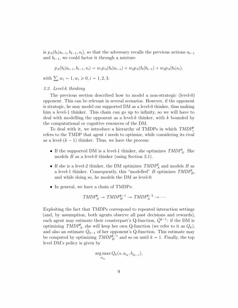
and so on, until we arrive at the induction basis (level-1) in which the opponentmay be modelled using the FPQ-learning approach in Section 3.1. Algorithm1 specifies the approach for a level-2 DM.

Therefore, we need to account for her Q-function, Q2, and that of heropponent (who will be level-1), Q1. Figure 1 provides a schematic view ofthe dependencies.

Algorithm 1 Level-2 thinking update rule

Require: Q2, Q1, α2, α1 (DM and opponent Q-functions and learning rates,respectively).Observe transition ps, a, b, rA, rB, s

1q

Q1ps, b, aq :“ p1´ α1qQ1ps, b, aq ` α1prB ` γmaxb1 EpBpa1|s1q”

Q1ps1, b1, a1q

ı

q

Compute B’s estimated ε´greedy policy pApb|s1q from Q1ps, b, aq

Q2ps, a, bq :“ p1´ α2qQ2ps, a, bq ` α2prA ` γmaxa1 EpApb1|s1q rQ2ps1, a1, b1qsq

Level-2 (DM, denoted as A)

Q2, pApb|sq ø Level-1 (Adv., denoted as B)

Q1, pBpa|sq ø Level-0 (DM)

Figure 1: Level-k thinking scheme, with k “ 2

Note that in the previous hierarchy of policies the decisions are obtainedin a greedy manner, by maximizing the lower level Q estimate. We may gaininsight in a Bayesian fashion by adding uncertainty to the policy at each level.For instance, at a certain level in the hierarchy, we could consider ε´greedypolicies that with probability 1´ ε choose an action according to the previousscheme and, with probability ε, select a random action. Thus, we may imposedistributions pkpεq at each level k of the hierarchy. The mean of pkpεq maybe an increasing function with respect to the level k to account for the factthat uncertainty is higher at the upper thinking levels.

10

3.3. Combining Opponent Models

We have discussed a hierarchy of opponent models. In most situations theDM will not know which type of particular opponent she is facing. To dealwith this, she may place a prior ppMiq denoting her beliefs that her opponentis using a model Mi, for i “ 1, . . . ,m, the range of models that might describeher adversary’s behavior, with

řmi“0 ppMiq “ 1.

As an example, she might place a Dirichlet prior. Then, at each iteration,after having observed her opponent’s action, she may update her belief ppMiq

by increasing the count of the model Mi which caused that action, as in thestandard Dirichlet-Categorical Bayesian update rule (Algorithm 2). This ispossible since the DM maintains an estimate of the opponent’s policy foreach opponent model Mi, denoted pMi

pb|sq. If none of the opponent modelshad predicted the observed action bt, then we may not perform an update(as stated in Algorithm 2 and done in the experiments) or we could increasethe count for all possible actions.

Algorithm 2 Opponent average updating

Require: ppM |Hq9 pn1, n2, . . . , nmq, where H is the sequencepb0, b1, . . . , bt´1q of past opponent actions.Observe transition pst, at, bt, rA,t, rB,t, st`1q.For each opponent model Mi, set bi to be the predicted action by modelMi.If bi “ bt then update posterior:

ppM |pH||btqq9 pn1, . . . , ni ` 1, . . . , nmq

Note that this model averaging scheme subsumes the framework of cogni-tive hierarchies [37], since a belief distribution is placed over the different levelsof the hierarchy. However, it is more flexible since more kinds of opponentscan be taken into account, for instance a minimax agent as exemplified in[34].

3.4. Facing multiple opponents

TMDPs may be extended to the case of a DM facing more than oneadversary. Then, the DM would have uncertainty about all of her opponentsand she would need to average her Q-function over all likely actions of alladversaries. Let pApb

1, . . . , bM |sq represent the DM’s beliefs about her M

11

adversaries’ actions. The extension of the TMDP framework to multipleadversaries will require to account for all possible opponents in the DM’s Qfunction taking the form Qps, a, b1, . . . , bMq. Finally, the DM would need toaverage this Q over b1, . . . , bM in (3) and proceed as in (4).

In case the DM is facing non-strategic opponents, she could learn pApb1, . . . ,

bM |sq in a Bayesian way, as explained in Section 3.1. This would entailplacing a Dirichlet prior on the nM dimensional vector of joint actions of alladversaries. However, keeping track of those probabilities may be unfeasibleas the dimension scales exponentially with the number of opponents. Thecase of conditionally independent adversaries turns out to be much simpleras we can use the fact that pApb

1, . . . , bM |sq “ pApb1|sq ¨ . . . pApb

M |sq. In thiscase, we could learn each pApb

i|sq for i “ 1, . . . ,M separately, as explained inprevious sections.

3.5. Computational complexity

As described before, a level-k Q-learner has to estimate the Q function ofa level-pk´ 1q Q-learner, and so on. Assuming the original Q-learning updaterule has time complexity OpT p|A|qq, with T being a factor depending on thenumber of actions of the DM, the update rule from Algorithm 1 has timecomplexity OpkT pmaxt|A|, |B|uqq, i.e., linear in the level of the hierarchy.

Regarding space complexity, the overhead is also linear in the level k sincethe DM only needs to store k Q-functions, so the complexity is OpkMp|S|, |A|¨|B|qq with Mp|S|, |A| ¨ |B|q accounting for the memory needed to store theQ-function in tabular form.

4. Experiments and Results

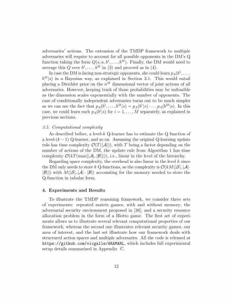
To illustrate the TMDP reasoning framework, we consider three setsof experiments: repeated matrix games, with and without memory; theadversarial security environment proposed in [38]; and a security resourceallocation problem in the form of a Blotto game. The first set of experi-ments allows us to illustrate several relevant computational properties of ourframework, whereas the second one illustrates relevant security games, ourarea of interest, and the last set illustrate how our framework deals withstructured action spaces and multiple adversaries. All the code is released athttps://github.com/vicgalle/ARAMARL, which includes full experimentalsetup details summarized in Appendix C.

12

4.1. Repeated Matrix Games

We first consider experiments with agents without memory, then agentswith memory, and, finally, discuss general conclusions. As initial baseline,we focus on the stateless version of a TMDP and analyze the policies learntby the DM, and analyze the policies learnt by the DM, who will be the rowplayer in the corresponding matrix game, against various kinds of opponents.In all the iterated games, agent i P tA,Bu aims at optimizing

ř8

t“0 γtrit, and

we set the discount factor γ “ 0.96 for illustration purposes.

4.1.1. Memoryless Repeated Matrix Games

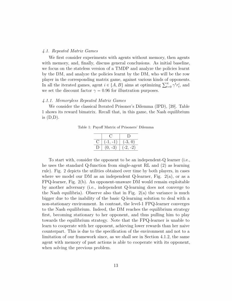
We consider the classical Iterated Prisoner’s Dilemma (IPD), [39]. Table1 shows its reward bimatrix. Recall that, in this game, the Nash equilibriumis (D,D).

Table 1: Payoff Matrix of Prisoners’ Dilemma

C DC (-1, -1) (-3, 0)D (0, -3) (-2, -2)

To start with, consider the opponent to be an independent-Q learner (i.e.,he uses the standard Q-function from single-agent RL and (2) as learningrule). Fig. 2 depicts the utilities obtained over time by both players, in caseswhere we model our DM as an independent Q-learner, Fig. 2(a), or as aFPQ-learner, Fig. 2(b). An opponent-unaware DM would remain exploitableby another adversary (i.e., independent Q-learning does not converge tothe Nash equilibria). Observe also that in Fig. 2(a) the variance is muchbigger due to the inability of the basic Q-learning solution to deal with anon-stationary environment. In contrast, the level-1 FPQ-learner convergesto the Nash equilibrium. Indeed, the DM reaches the equilibrium strategyfirst, becoming stationary to her opponent, and thus pulling him to playtowards the equilibrium strategy. Note that the FPQ-learner is unable tolearn to cooperate with her opponent, achieving lower rewards than her naivecounterpart. This is due to the specification of the environment and not to alimitation of our framework since, as we shall see in Section 4.1.2, the sameagent with memory of past actions is able to cooperate with its opponent,when solving the previous problem.

13

(a) Q-learner vs Q-learner (b) FPQ-learner (blue) vs Q-learner (red)

Figure 2: Rewards obtained in IPD. We plot the trajectories of 10 simulations with shadedcolors. Darker curves depict mean rewards.

(a) Q-learner vs Q-learner (b) FPQ-learner (blue) vs Q-learner (red)

Figure 3: Rewards in ISH game

(a) Q-learner vs Q-learner (b) FPQ-learner (blue) vs Q-learner (red)

Figure 4: Rewards in IC game

14

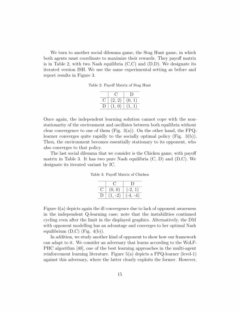
We turn to another social dilemma game, the Stag Hunt game, in whichboth agents must coordinate to maximize their rewards. They payoff matrixis in Table 2, with two Nash equilibria (C,C) and (D,D). We designate itsiterated version ISH. We use the same experimental setting as before andreport results in Figure 3.

Table 2: Payoff Matrix of Stag Hunt

C DC (2, 2) (0, 1)D (1, 0) (1, 1)

Once again, the independent learning solution cannot cope with the non-stationarity of the environment and oscillates between both equilibria withoutclear convergence to one of them (Fig. 3(a)). On the other hand, the FPQ-learner converges quite rapidly to the socially optimal policy (Fig. 3(b)).Then, the environment becomes essentially stationary to its opponent, whoalso converges to that policy.

The last social dilemma that we consider is the Chicken game, with payoffmatrix in Table 3. It has two pure Nash equilibria (C, D) and (D,C). Wedesignate its iterated variant by IC.

Table 3: Payoff Matrix of Chicken

C DC (0, 0) (-2, 1)D (1, -2) (-4, -4)

Figure 4(a) depicts again the ill convergence due to lack of opponent awarenessin the independent Q-learning case; note that the instabilities continuedcycling even after the limit in the displayed graphics. Alternatively, the DMwith opponent modelling has an advantage and converges to her optimal Nashequilibrium (D,C) (Fig. 4(b)).

In addition, we study another kind of opponent to show how our frameworkcan adapt to it. We consider an adversary that learns according to the WoLF-PHC algorithm [40], one of the best learning approaches in the multi-agentreinforcement learning literature. Figure 5(a) depicts a FPQ-learner (level-1)against this adversary, where the latter clearly exploits the former. However,

15

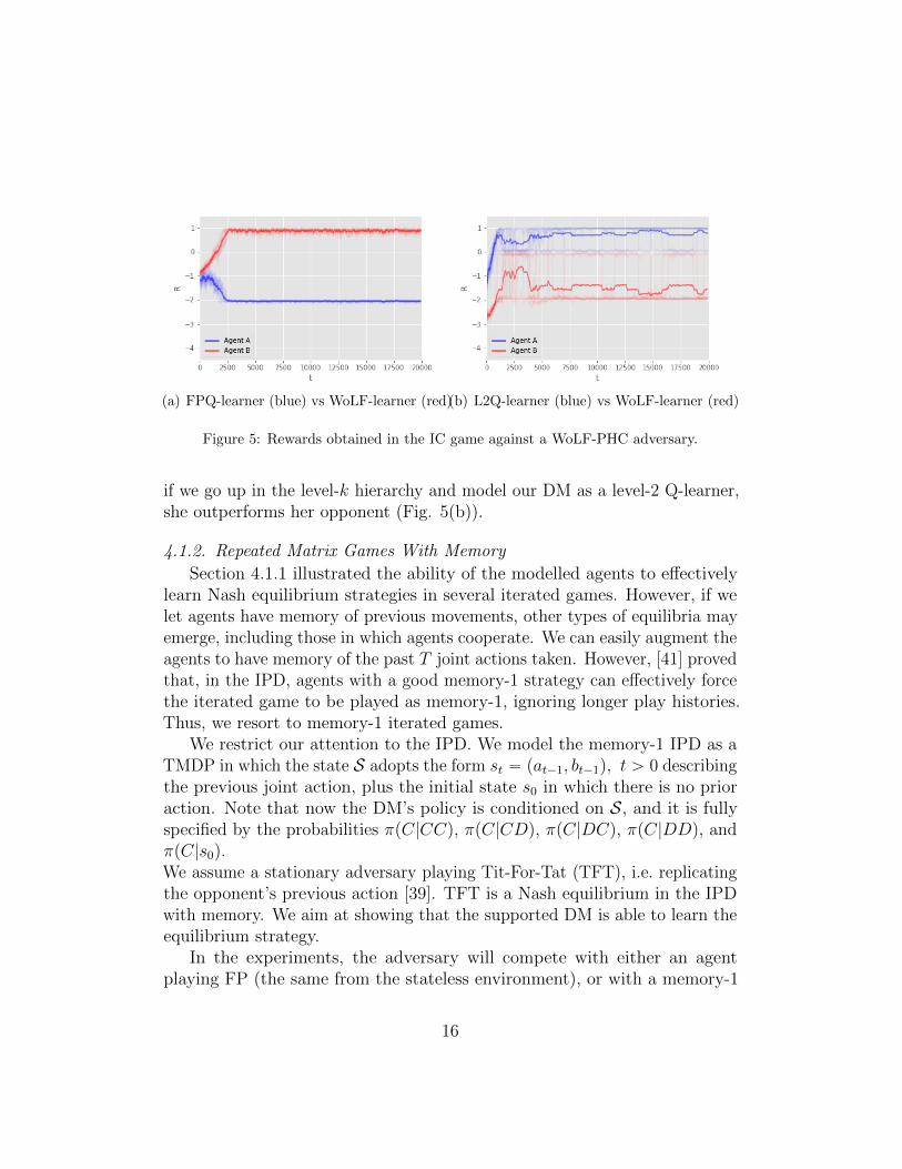
(a) FPQ-learner (blue) vs WoLF-learner (red)(b) L2Q-learner (blue) vs WoLF-learner (red)

Figure 5: Rewards obtained in the IC game against a WoLF-PHC adversary.

if we go up in the level-k hierarchy and model our DM as a level-2 Q-learner,she outperforms her opponent (Fig. 5(b)).

4.1.2. Repeated Matrix Games With Memory

Section 4.1.1 illustrated the ability of the modelled agents to effectivelylearn Nash equilibrium strategies in several iterated games. However, if welet agents have memory of previous movements, other types of equilibria mayemerge, including those in which agents cooperate. We can easily augment theagents to have memory of the past T joint actions taken. However, [41] provedthat, in the IPD, agents with a good memory-1 strategy can effectively forcethe iterated game to be played as memory-1, ignoring longer play histories.Thus, we resort to memory-1 iterated games.

We restrict our attention to the IPD. We model the memory-1 IPD as aTMDP in which the state S adopts the form st “ pat´1, bt´1q, t ą 0 describingthe previous joint action, plus the initial state s0 in which there is no prioraction. Note that now the DM’s policy is conditioned on S, and it is fullyspecified by the probabilities πpC|CCq, πpC|CDq, πpC|DCq, πpC|DDq, andπpC|s0q.We assume a stationary adversary playing Tit-For-Tat (TFT), i.e. replicatingthe opponent’s previous action [39]. TFT is a Nash equilibrium in the IPDwith memory. We aim at showing that the supported DM is able to learn theequilibrium strategy.

In the experiments, the adversary will compete with either an agentplaying FP (the same from the stateless environment), or with a memory-1

16

Figure 6: Rewards obtained by the DM for players: FPQ memoryless player vs TFT player(G1) and FPQ memory-1 player vs TFT player (G2).

agent also playing FP. Figure 6 represents the utilities attained by theseagents in both duels. As can be seen, a memoryless FPQ player cannotlearn an optimal policy and forces the TFT agent to play defect. In contrast,augmenting this agent to have memory of the previous move allows him tolearn the optimal policy (TFT), that is, he learns to cooperate, leading to ahigher cumulative reward.

4.1.3. Discussion

We have shown through our examples some qualitative properties of theproposed framework. Explicitly modelling an opponent (as in the level-1 orFPQ-learner) is beneficial to maximize the rewards attained by the DM, asshown in the ISH and IC games. In both games, the DM obtains higher rewardas a level-1 thinker than as a naive Q-learner against the same opponent.Also, going up in the hierarchy helps the DM to cope with more powerfulopponents such as the WoLF-PHC algorithm.

In the two previous games, a level-1 DM makes both her and her opponentreach a Nash equilibrium, in contrast with the case in which the DM is anaive learner, where clear convergence is not assured. In both games thereexist two pure Nash equilibria, and the higher-level DM achieved the mostprofitable one for her, effectively exploiting her adversary.

The case of the IPD is specially interesting. Though the level-1 DM alsoconverges to the unique Nash equilibrium (Fig. 2(b)), it obtains less rewardthan its naive counterpart (Fig. 2(a)). Recall that the naive Q-learner wouldremain exploitable by another opponent. We argue that the FPQ-learner

17

did not learn to cooperate, and thus achieves lower rewards, due to thespecification of the game and not as a limitation of our approach. To allowfor the emergence of cooperation in the IPD, agents should remember pastactions taken by all players. If we specify an environment in which agentsrecall the last pair of actions taken, the FPQ-learner is able to cooperate (Fig.6) with an opponent that plays a Nash optimum strategy in this modifiedsetting, Tit-For-Tat.

4.2. AI Safety Gridworlds and Markov Security Games

A suite of RL safety benchmarks has been recently introduced in [38]. Wefocus on the safety friend or foe environment, in which the supported DMneeds to travel a room and choose between two identical boxes, hiding positiveand negative rewards, respectively. The reward assignment is controlled byan adaptive opponent. Figure 7 shows the initial state in this game. The bluecell depicts the DM’s initial state, gray cells represent the walls of the room.Cells 1 and 2 depict the adversary’s targets, who decides which one will hidethe positive reward. This case may be interpreted as a spatial Stackelberggame in which the adversary is planning to attack one of two targets, andthe defender will obtain a positive reward if she travels to the chosen target.Otherwise, she will miss the attacker and will incur in a loss.

As shown in [38], a deep Q-network (and, similarly, the independenttabular Q-learner as we show) fails to achieve optimal results because thereward process is controlled by the adversary. By explicitly modelling it, weactually improve Q-learning methods achieving better rewards. An alternativeapproach to security games in spatial domains was introduced in [42]. Theauthors extend the single-agent Q-learning algorithm with an adversarialpolicy selection inspired by the EXP3 rule from the adversarial multi-armedbandit framework in [26]. However, although robust, their approach doesnot explicitly model an adversary. We demonstrate that by modelling anopponent the DM can achieve higher rewards.

4.2.1. Stateless Variant

We first consider a simplified environment with a singleton state and twoactions. In a spirit similar to [38], the adaptive opponent estimates the DM’sactions using an exponential smoother. Let p “ pp1, p2q be the probabilitieswith which the DM will, respectively, choose targets 1 or 2 as estimated by theopponent. At every iteration, the opponent updates his knowledge through

p :“ βp` p1´ βqa,

18

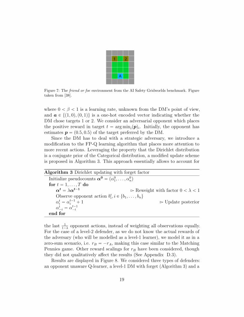
Figure 7: The friend or foe environment from the AI Safety Gridworlds benchmark. Figuretaken from [38].

where 0 ă β ă 1 is a learning rate, unknown from the DM’s point of view,and a P tp1, 0q, p0, 1qu is a one-hot encoded vector indicating whether theDM chose targets 1 or 2. We consider an adversarial opponent which placesthe positive reward in target t “ arg minippqi. Initially, the opponent hasestimates p “ p0.5, 0.5q of the target preferred by the DM.

Since the DM has to deal with a strategic adversary, we introduce amodification to the FP-Q learning algorithm that places more attention tomore recent actions. Leveraging the property that the Dirichlet distributionis a conjugate prior of the Categorical distribution, a modified update schemeis proposed in Algorithm 3. This approach essentially allows to account for

Algorithm 3 Dirichlet updating with forget factor

Initialize pseudocounts α0 “ pα01, . . . , α

0nq

for t “ 1, . . . , T doαt “ λαt´1 Ź Reweight with factor 0 ă λ ă 1Observe opponent action bti, i P tb1, . . . , bnuαti “ αt´1i ` 1 Ź Update posteriorαt´i “ αt´1´i

end for

the last 11´λ

opponent actions, instead of weighting all observations equally.For the case of a level-2 defender, as we do not know the actual rewards ofthe adversary (who will be modelled as a level-1 learner), we model it as in azero-sum scenario, i.e. rB “ ´rA, making this case similar to the MatchingPennies game. Other reward scalings for rB have been considered, thoughthey did not qualitatively affect the results (See Appendix D.3).

Results are displayed in Figure 8. We considered three types of defenders:an opponent unaware Q-learner, a level-1 DM with forget (Algorithm 3) and a

19

Figure 8: Rewards for the DM against the adversarial opponent

level-2 agent. The first one is exploited by the adversary achieving suboptimalresults. In contrast, the level-1 DM with forget effectively learns a stationaryoptimal policy (reward 0). Finally, the level-2 agent learns to exploit theadaptive adversary achieving positive rewards.

Note that the actual adversary behaves differently from how the DMmodels him, i.e. he is not exactly a level-1 Q-learner. Even so, modelling himas a level-1 agent gives the DM sufficient advantage.

4.2.2. Facing more powerful adversaries

Until now the DM has interacted against an exponential smoother adver-sary, which may be exploited if the DM is a level-2 agent. We study now theoutcome of the process if we consider more powerful adversaries.

First of all, we parameterize our opponent as a level-2 Q-learner, insteadof the exponential smoother. To do so, we specify the rewards he shallreceive as rB “ ´rA, i.e., for simplicity we consider a zero-sum game, yet ourframework allows for the general-sum case. Figure 9(a) depicts the rewardsfor both the DM (blue) and the adversary (red). We have computed thefrequency for choosing each action, and both players select either action withprobability 0.5˘ 0.002 along 10 different random seeds. Both agents achievethe Nash equilibrium, consisting of choosing between both actions with equalprobabilities, leading to an expected cumulative reward of 0, as shown in thegraph.

Increasing the level of our DM to make her level-3, allows her to exploita level-2 adversary, Fig. 9(b). However, this DM fails to exploit a level-1

20

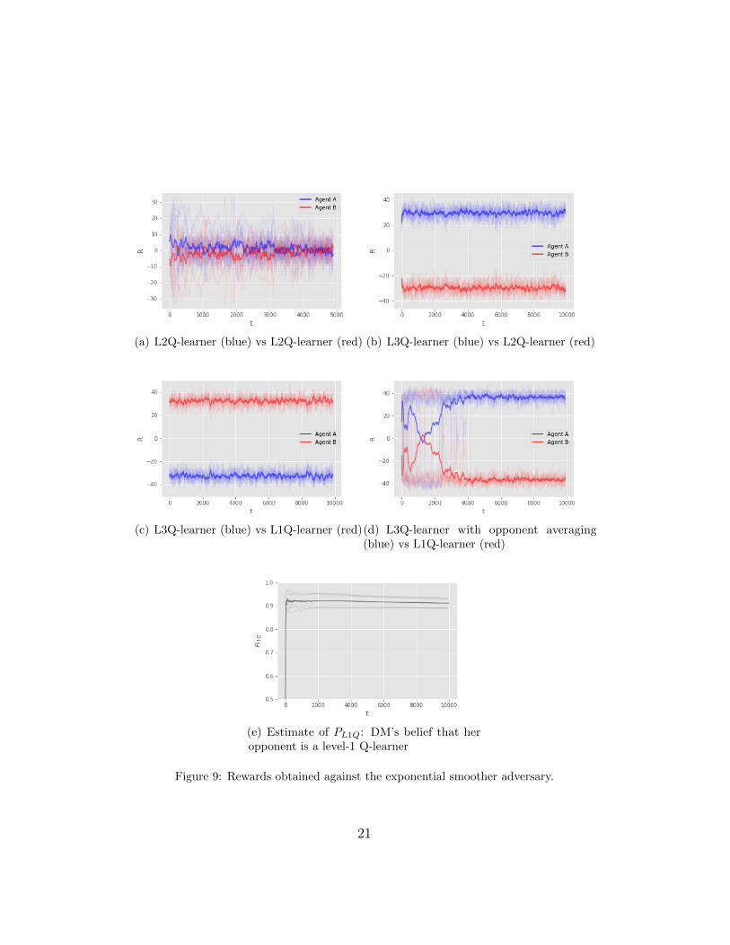
(a) L2Q-learner (blue) vs L2Q-learner (red) (b) L3Q-learner (blue) vs L2Q-learner (red)

(c) L3Q-learner (blue) vs L1Q-learner (red)(d) L3Q-learner with opponent averaging(blue) vs L1Q-learner (red)

(e) Estimate of PL1Q: DM’s belief that heropponent is a level-1 Q-learner

Figure 9: Rewards obtained against the exponential smoother adversary.

21

opponent (i.e., a FPQ-learner), Fig. 9(c). The explanation to this apparentparadox is that the DM is modelling her opponent as a more powerful agentthan he actually is, so her model is inaccurate and leads to poor performance.However, the previous “failure” suggests a potential solution to the problemusing type-based reasoning, Section 3.3. Figure 9(d) depicts the rewardsof a DM that keeps track of both level-1 and level-2 opponent models andlearns, in a Bayesian manner, which one is she actually facing. The DM keepsestimates of the probabilities PL1Q and PL2Q that her opponent is acting as ifhe was a level-1 or a level-2 Q-learner, respectively. Figure 9(e) depicts theevolution of PL1Q, and we can observe that it places most of the probabilityin the correct opponent type.

4.2.3. Spatial Variant

We now compare the independent Q-learner and a level-2 Q-learner againstthe same adaptive opponent (exponential smoother) in the spatial gridworlddomain, see Fig. 7. Target rewards are delayed until the DM arrives at oneof the respective locations, obtaining ˘50 depending on the target chosenby the adversary. Each step is penalized with a reward of -1 for the DM.Results are displayed in Figure 10(a). Once again, the independent Q-learneris exploited by the adversary, obtaining even more negative rewards than inFigure 8 due to the penalty taken at each step. In contrast, the level-2 agentis able to approximately estimate the adversarial behavior, modelling himas a level-1 agent, thus being able to obtain positive rewards. Figure 10(b)depicts rewards of a DM that keeps opponent models for both level-1 andlevel-2 Q-learners. Note that although the adversary is of neither class, theDM achieves positive rewards, suggesting that the framework is capable ofgeneralizing between different model opponents.

4.3. TMDPs for Security Resource Allocation

We illustrate the multiple opponent concepts of Section 3.4 introducing anovel suite of resource allocation experiments which are relevant in securitysettings. We propose a modified version of Blotto games [43]: the DM needsto distribute limited resources over several positions which are susceptible ofbeing attacked. In the same way, each of the attackers has to choose differentpositions where they can deploy their attacks. Associated with each of theattacked positions there is a positive (negative) reward of value 1 (-1). Ifthe DM deploys more resources than the attacks deployed in a particularposition, she wins the positive reward; the negative reward will be equally

22

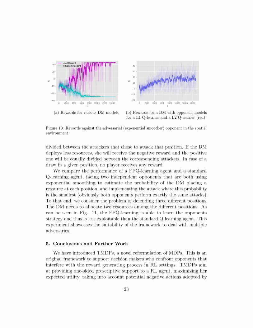
(a) Rewards for various DM models (b) Rewards for a DM with opponent modelsfor a L1 Q-learner and a L2 Q-learner (red)

Figure 10: Rewards against the adversarial (exponential smoother) opponent in the spatialenvironment.

divided between the attackers that chose to attack that position. If the DMdeploys less resources, she will receive the negative reward and the positiveone will be equally divided between the corresponding attackers. In case of adraw in a given position, no player receives any reward.

We compare the performance of a FPQ-learning agent and a standardQ-learning agent, facing two independent opponents that are both usingexponential smoothing to estimate the probability of the DM placing aresource at each position, and implementing the attack where this probabilityis the smallest (obviously both opponents perform exactly the same attacks).To that end, we consider the problem of defending three different positions.The DM needs to allocate two resources among the different positions. Ascan be seen in Fig. 11, the FPQ-learning is able to learn the opponentsstrategy and thus is less exploitable than the standard Q-learning agent. Thisexperiment showcases the suitability of the framework to deal with multipleadversaries.

5. Conclusions and Further Work

We have introduced TMDPs, a novel reformulation of MDPs. This is anoriginal framework to support decision makers who confront opponents thatinterfere with the reward generating process in RL settings. TMDPs aimat providing one-sided prescriptive support to a RL agent, maximizing herexpected utility, taking into account potential negative actions adopted by

23

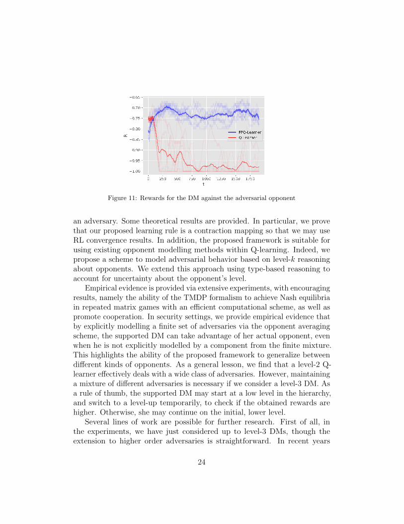
Figure 11: Rewards for the DM against the adversarial opponent

an adversary. Some theoretical results are provided. In particular, we provethat our proposed learning rule is a contraction mapping so that we may useRL convergence results. In addition, the proposed framework is suitable forusing existing opponent modelling methods within Q-learning. Indeed, wepropose a scheme to model adversarial behavior based on level-k reasoningabout opponents. We extend this approach using type-based reasoning toaccount for uncertainty about the opponent’s level.

Empirical evidence is provided via extensive experiments, with encouragingresults, namely the ability of the TMDP formalism to achieve Nash equilibriain repeated matrix games with an efficient computational scheme, as well aspromote cooperation. In security settings, we provide empirical evidence thatby explicitly modelling a finite set of adversaries via the opponent averagingscheme, the supported DM can take advantage of her actual opponent, evenwhen he is not explicitly modelled by a component from the finite mixture.This highlights the ability of the proposed framework to generalize betweendifferent kinds of opponents. As a general lesson, we find that a level-2 Q-learner effectively deals with a wide class of adversaries. However, maintaininga mixture of different adversaries is necessary if we consider a level-3 DM. Asa rule of thumb, the supported DM may start at a low level in the hierarchy,and switch to a level-up temporarily, to check if the obtained rewards arehigher. Otherwise, she may continue on the initial, lower level.

Several lines of work are possible for further research. First of all, inthe experiments, we have just considered up to level-3 DMs, though theextension to higher order adversaries is straightforward. In recent years

24

Q-learning has benefited from advances from the deep learning community,with breakthroughs such as the deep Q-network (DQN) which achieved super-human performance in control tasks such as the Atari games [13], or asinner blocks inside systems that play Go [14]. Integrating these advancesinto the TMDP setting is another possible research path. In particular, theproposed Algorithm 1 can be generalized to account for the use of deepQ-networks instead of tabular Q-learning as presented here. We show detailsof the modified algorithm in Appendix B. Indeed, the proposed schemeis model agnostic, i.e., it does not matter if we represent the Q-functionusing a look-up table or a deep neural network, so we expect it to be usablein both shallow and deep multi-agent RL settings. In addition, there areseveral other ways to model the adversary’s behavior that do not require tolearn opponent Q-values, for instance by using policy gradient methods [44].Finally, it might be interesting to explore similar expansions to semi-MDPs,in order to perform hierarchical RL or to allow for time-dependent rewardsand transitions between states.

Acknowledgements. VG acknowledges support from grant FPU16-05034, RN acknowledges support from the Spanish Ministry for his grantFPU15-03636. DRI is grateful to the MINCIU MTM2017-86875-C3-1-Rproject and the AXA-ICMAT Chair in Adversarial Risk Analysis. All authorsacknowledge support from the Severo Ochoa Excellence Programme SEV-2015-0554. We are also very grateful to the numerous pointers and suggestionsby the referees. This version of the manuscript was prepared while the authorswere visiting SAMSI within the Games and Decisions in Risk and Reliabilityprogram.

25

Appendix A. Sketch of proof of convergence of the update rulefor TDMPs (Eqs. (3) and (4))

Consider an augmented state space so that transitions are of the form

ps, bqaÝÑ ps1, b1q

a1ÝÑ . . . .

Under this setting, the DM does not observe the full state since she doesnot know the action b taken by her adversary. However, if she knows hispolicy ppb|sq, or has a good estimate of it, she can take advantage of thisinformation.

Assume for now that we know the current opponent’s action b. TheQ-function would satisfy the following recursive update [19],

Qπps, a, bq “

ř

s1

ř

b1 pps1, b1|s, a, bq

“

Rabss1 ` Eπpa1|s1,b1q rQπps1, a1, b1qs

‰

,

where we have taken into account explicitly the structure of the state spaceand used Rab

ss1 “ E rrt`1|st`1 “ s1, st “ s, at “ a, bt “ bs. As the next oppo-nent action is conditionally independent of his previous action, the previousDM action and the previous state, given the current state, we may writepps1, b1|s, a, bq “ ppb1|s1qpps1|s, a, bq. Thus

Qπps, a, bq “

ř

s1 pps1|s, a, bq

“

Rabss1 ` Eppb1|s1qEπpa1|s1,b1q rQπps1, a1, b1qs

‰

as Rabss1 does not depend on the next opponent action b1. Finally, the optimal

Q-function verifies

Q˚ps, a, bq “ÿ

s1

pps1|s, a, bq”

Rabss1 ` γmax

a1Eppb1|s1q rQ˚ps1, a1, b1qs

ı

,

since in this case πpa|sq “ arg maxaQ˚ps, aq. Observe now that:

Lemma 1. Given q : S ˆ B ˆAÑ R, the operator H

pHqqps, b, aq “ÿ

s1

pps1|s, b, aq“

rps, b, aq ` γmaxa1

Eppb1|s1qqps1, b1, a1q‰

.

is a contraction mapping under the supremum norm.

26

Proof. We prove that }Hq1 ´Hq2}8 ď γ}q1 ´ q2}8.

}Hq1 ´Hq2}8 ““ max

s,b,a|ÿ

s1

pps1|s, b, aq“

rps, b, aq ` γmaxa1

Eppb1|s1qq1ps1, b1, a1q

´ rps, b, aq ´ γmaxa1

Eppb1|s1qq2ps1, b1, a1q‰

| “

“ γmaxs,b,a|ÿ

s1

pps1|s, b, aq“

maxa1

Eppb1|s1qq1ps1, b1, a1q

´maxa1

Eppb1|s1qq2ps1, b1, a1q‰

| ď

“ γmaxs,b,a

ÿ

s1

pps1|s, b, aq|maxa1

Eppb1|s1qq1ps1, b1, a1q

´maxa1

Eppb1|s1qq2ps1, b1, a1q| ď

“ γmaxs,b,a

ÿ

s1

pps1|s, b, aqmaxa1,z|Eppb1|zqq1pz, b1, a1q

´ Eppb1|zqq2pz, b1, a1q| ď“ γmax

s,b,a

ÿ

s1

pps1|s, b, aqmaxa1,z,b1|q1pz, b1, a1q ´ q2pz, b1, a1q| “

“ γmaxs,b,a

ÿ

s1

pps1|s, b, aq}q1 ´ q2}8 “

“ γ}q1 ´ q2}8.

Then, using the proposed learning rule (3), we would converge to the optimalQ for each of the opponent actions. The proof follows directly from thestandard Q-learning convergence proof, see e.g. [45], and making use of theprevious Lemma.

However, at the time of making the decision, we do not know what actionhe would take. Thus, we suggest to average over the possible opponent actions,weighting each by ppb|sq, as in (4).

Appendix B. Generalization to deep-Q learning

The tabular version of Q-learning introduced in Algorithm 1 does notscale well when the state or action spaces dramatically grow in size. To this

27

end, we expand the framework to the case when the Q-functions are insteadrepresented using a function approximator, typically a deep Q-network [13].Algorithm 4 shows the details. The parameters φA and φB refer to the weightsof the corresponding networks approximating the Q-values.

Algorithm 4 Level-2 thinking update rule using neural approximators.

Require: QφA , QφB , α2, α1 (DM and opponent Q-functions and learningrates, respectively).Observe transition ps, a, b, rA, rB, s

1q.

φB :“ φB´α1BQφBBφB

ps, b, aq“

QφBps, b, aq ´ prB ` γmaxb1 EpBpa1|s1qQφBps1, b1, a1qq

‰

Compute B’s estimated ε´greedy policy pApb|s1q from QφBps, b, aq.

φA :“ φA´α2BQφABφA

ps, a, bq“

QφAps, a, bq ´ prA ` γmaxa1 EpApb1|s1qQφAps1, a1, b1qq

‰

Appendix C. Experiment Details

We describe hyperparameters and other technical details used in theexperiments.

Repeated matrix games

Memoryless Repeated Matrix Games

In all three games (IPD, ISH, IC) we considered a discount factor γ “ 0.96,a total of max steps T “ 20000, initial ε “ 0.1 and learning rate α “ 0.3. TheFP-Q learner started the learning process with a Beta prior Bp1, 1q.

Repeated Matrix Games With Memory

In the IPD game we considered a discount factor γ “ 0.96, a total of maxsteps T “ 20000, initial ε “ 0.1 and learning rate α “ 0.05. The FP-Q learnerstarted the learning process with a Beta prior Bp1, 1q.

AI Safety Gridworlds

Stateless Variant

Rewards for the DM are 50,´50 depending on her action and the targetchosen by the adversary. We considered a discount factor γ “ 0.8 and a totalof 5000 episodes. For all three agents, the initial exploration parameter wasset to ε “ 0.1 and learning rate α “ 0.1. The FP-Q learner with forget factorused λ “ 0.8.

28

Spatial Variant

Episodes end at a maximum of 50 steps or agent arriving first at target1 or 2. Rewards for the DM are ´1 for performing any action (i.e., a stepin some of the four possible directions) or 50,´50 depending on the targetchosen by the adversary. We considered a discount factor γ “ 0.8 and a totalof 15000 episodes. For the level-2 agent, initial εA “ εB “ 0.99 with decayingrules εA :“ 0.995εA and εB :“ 0.9εB every 10 episodes and learning ratesα2 “ α1 “ 0.05. For the independent Q-learner we set initial exploration rateε “ 0.99 with decaying rule ε :“ 0.995ε every 10 episodes and learning rateα “ 0.05.

TMDPs for Security Resource Allocation

For both the Q-learning and the FPQ-learning agents we considered adiscount factor γ “ 0.96, ε “ 0.1 and a learning rate of 0.1.

Appendix D. Additional Results

Appendix D.1. Alternative policies

Although we have focused in pure strategies, dealing with mixed onesis straightforward as it just entails changing the ε´greedy policy with thesoftmax policy.

In this Appendix we perform an experiment in which we replace theε´greedy policy of the DM with a softmax policy in the spatial gridworldenvironment from Section 4.2. Actions at state s are taken with probabilityproportional to Qps, aq. See Figure D.12 for several simulation runs of a level-2 Q-learner versus the adversary, showing that indeed changing the policysampling scheme does not make the DM worse than its ε´greedy alternative.

Appendix D.2. Robustness to hyperparameters

We perform several experiments in which we try different values of thehyperparameters, just to highlight the robustness of the framework. TableD.4 displays mean rewards (and standard deviations) for five different randomseeds, over different hyperparameters of Algorithm 1. Except in the casewhere the initial exploration rate ε0 is set to a high value (0.5, which makesthe DM to achieve a positive mean reward), the other settings showcase thatthe framework (for the level-2 case) is robust to different learning rates.

29

Figure D.12: Rewards for the DM against the adversarial opponent, using a softmax policy.

Table D.4: Results on hyperparameter robustness of Algorithm 1 on the spatial gridworld.

α2 α1 ε0 Mean Reward0.01 0.005 0.5 15.46˘ 47.210.01 0.005 0.1 40.77˘ 27.480.01 0.005 0.01 46.32˘ 16.150.01 0.02 0.5 15.58˘ 47.170.01 0.02 0.1 43.05˘ 23.650.01 0.02 0.01 47.81˘ 10.830.1 0.05 0.5 15.30˘ 47.270.1 0.05 0.1 42.82˘ 24.080.1 0.05 0.01 48.34˘ 8.100.1 0.2 0.5 15.97˘ 47.030.1 0.2 0.1 43.05˘ 23.660.1 0.2 0.01 48.51˘ 6.960.5 0.25 0.5 15.95˘ 47.040.5 0.25 0.1 43.06˘ 23.640.5 0.25 0.01 48.41˘ 7.680.5 1.0 0.5 15.19˘ 47.310.5 1.0 0.1 42.98˘ 23.710.5 1.0 0.01 48.53˘ 6.82

30

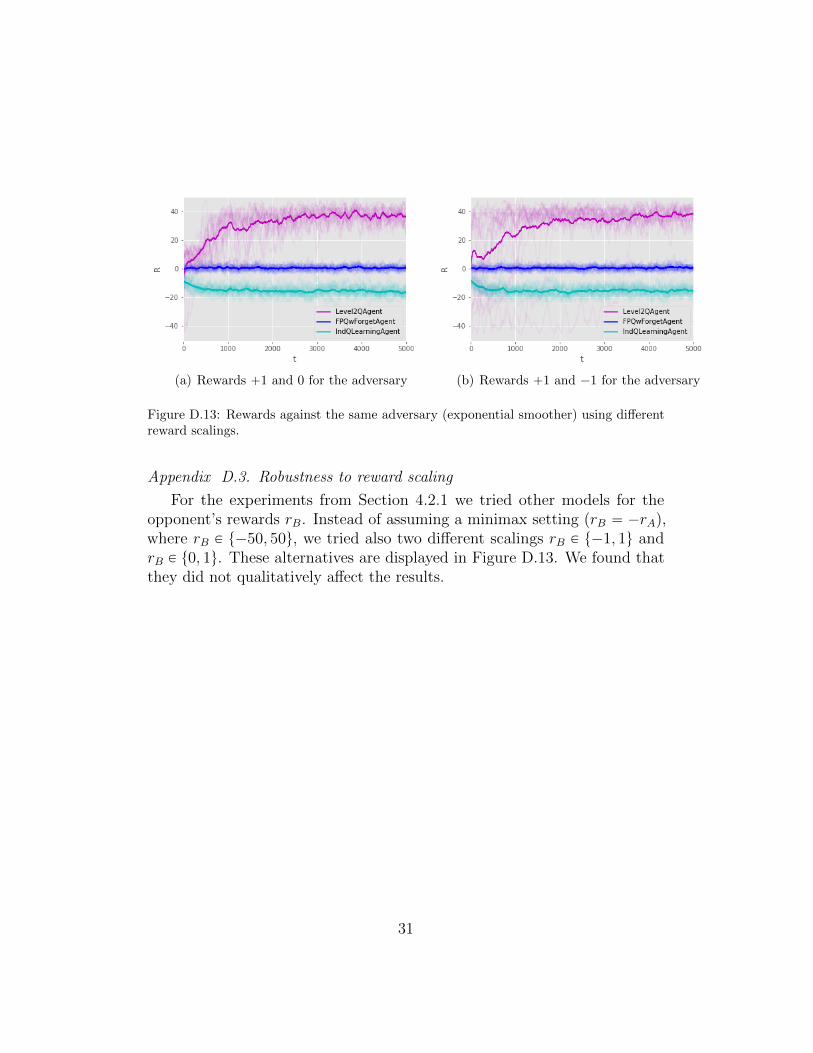
(a) Rewards `1 and 0 for the adversary (b) Rewards `1 and ´1 for the adversary

Figure D.13: Rewards against the same adversary (exponential smoother) using differentreward scalings.

Appendix D.3. Robustness to reward scaling

For the experiments from Section 4.2.1 we tried other models for theopponent’s rewards rB. Instead of assuming a minimax setting (rB “ ´rA),where rB P t´50, 50u, we tried also two different scalings rB P t´1, 1u andrB P t0, 1u. These alternatives are displayed in Figure D.13. We found thatthey did not qualitatively affect the results.

31

References

References

[1] I. J. Goodfellow, J. Shlens, C. Szegedy, Explaining and harnessingadversarial examples, arXiv preprint arXiv:1412.6572 (2014).

[2] J. G. Carbonell, Introduction:paradigms for machine learning, ArtificialIntelligence 40 (1989) 1 – 9.

[3] S. V. Albrecht, P. Stone, Autonomous agents modelling other agents:A comprehensive survey and open problems, Artif. Intell. 258 (2018)66–95.

[4] N. Dalvi, P. Domingos, S. Sanghai, D. Verma, et al., Adversarialclassification, in: Proceedings of the tenth ACM SIGKDD internationalconference on Knowledge discovery and data mining, ACM, 2004, pp.99–108.

[5] I. Menache, A. Ozdaglar, Network games: Theory, models, and dynamics,Synthesis Lectures on Communication Networks 4 (2011) 1–159.

[6] B. Biggio, F. Roli, Wild patterns: Ten years after the rise of adversarialmachine learning, Pattern Recognition 84 (2018) 317 – 331.

[7] Y. Zhou, M. Kantarcioglu, B. Xi, A survey of game theoretic approachfor adversarial machine learning, Wiley Interdisciplinary Reviews: DataMining and Knowledge Discovery (2018) e1259.

[8] S. Hargreaves-Heap, Y. Varoufakis, Game Theory: A Critical Introduc-tion, Taylor & Francis, 2004.

[9] R. Naveiro, A. Redondo, D. R. Insua, F. Ruggeri, Adversarial classifi-cation: An adversarial risk analysis approach, International Journal ofApproximate Reasoning (2019).

[10] D. R. Insua, J. Rios, D. Banks, Adversarial risk analysis, Journal of theAmerican Statistical Association 104 (2009) 841–854.

[11] J. B. Kadane, P. D. Larkey, Subjective probability and the theory ofgames, Management Science 28 (1982) 113–120.

32

[12] H. Raiffa, The Art and Science of Negotiation, Belknap Press of HarvardUniversity Press, 1982.

[13] V. Mnih, K. Kavukcuoglu, D. Silver, A. A. Rusu, J. Veness, M. G.Bellemare, A. Graves, M. Riedmiller, A. K. Fidjeland, G. Ostrovski,et al., Human-level control through deep reinforcement learning, Nature518 (2015) 529.

[14] D. Silver, J. Schrittwieser, K. Simonyan, I. Antonoglou, A. Huang,A. Guez, T. Hubert, L. Baker, M. Lai, A. Bolton, et al., Mastering thegame of go without human knowledge, Nature 550 (2017) 354.

[15] S. Huang, N. Papernot, I. Goodfellow, Y. Duan, P. Abbeel, Adversarialattacks on neural network policies, arXiv preprint arXiv:1702.02284(2017).

[16] Y.-C. Lin, Z.-W. Hong, Y.-H. Liao, M.-L. Shih, M.-Y. Liu, M. Sun,Tactics of adversarial attack on deep reinforcement learning agents,arXiv preprint arXiv:1703.06748 (2017).

[17] L. Busoniu, R. Babuska, B. De Schutter, Multi-agent reinforcementlearning: An overview, in: Innovations in multi-agent systems andapplications-1, Springer, 2010, pp. 183–221.

[18] R. A. Howard, Dynamic Programming and Markov Processes, MIT Press,Cambridge, MA, 1960.

[19] R. S. Sutton, A. G. Barto, Reinforcement learning: An introduction,MIT press, 2018.

[20] G. W. Brown, Iterative solution of games by fictitious play, ActivityAnalysis of Production and Allocation (1951) 374–376.

[21] J. Rios, D. R. Insua, Adversarial risk analysis for counterterrorismmodeling, Risk Analysis: An International Journal 32 (2012) 894–915.

[22] D. O. Stahl, P. W. Wilson, Experimental evidence on players’ models ofother players, Journal of economic behavior & organization 25 (1994)309–327.

33

[23] M. L. Littman, Markov games as a framework for multi-agent reinforce-ment learning, in: Machine Learning Proceedings 1994, Elsevier, 1994,pp. 157–163.

[24] J. Hu, M. P. Wellman, Nash Q-learning for general-sum stochastic games,Journal of machine learning research 4 (2003) 1039–1069.

[25] M. L. Littman, Friend-or-Foe Q-learning in General-Sum Games, in:Proceedings of the Eighteenth International Conference on MachineLearning, Morgan Kaufmann Publishers Inc., 2001, pp. 322–328.

[26] P. Auer, N. Cesa-Bianchi, Y. Freund, R. E. Schapire, Gambling in a riggedcasino: The adversarial multi-armed bandit problem, in: Foundationsof Computer Science, 1995. Proceedings., 36th Annual Symposium on,IEEE, 1995, pp. 322–331.

[27] M. Lanctot, V. Zambaldi, A. Gruslys, A. Lazaridou, K. Tuyls, J. Perolat,D. Silver, T. Graepel, A unified game-theoretic approach to multiagentreinforcement learning, in: Advances in Neural Information ProcessingSystems, 2017, pp. 4190–4203.

[28] P. J. Gmytrasiewicz, P. Doshi, A framework for sequential planning inmulti-agent settings, Journal of Artificial Intelligence Research 24 (2005)49–79.

[29] H. He, J. Boyd-Graber, K. Kwok, H. Daume III, Opponent modeling indeep reinforcement learning, in: International Conference on MachineLearning, 2016, pp. 1804–1813.

[30] J. Foerster, R. Y. Chen, M. Al-Shedivat, S. Whiteson, P. Abbeel, I. Mor-datch, Learning with opponent-learning awareness, in: Proceedings ofthe 17th International Conference on Autonomous Agents and Multi-Agent Systems, International Foundation for Autonomous Agents andMultiagent Systems, 2018, pp. 122–130.

[31] D. O. Stahl, P. W. Wilson, On players’ models of other players: Theoryand experimental evidence, Games and Economic Behavior 10 (1995)218–254.

[32] E. Altman, Constrained Markov Decision Processes, volume 7, CRCPress, 1999.

34

[33] A. M. Metelli, M. Mutti, M. Restelli, Configurable Markov Deci-sion Processes, International Conference on Machine Learning (2018).arXiv:1806.05415.

[34] D. R. Insua, D. Banks, J. Rios, Modeling opponents in adversarial riskanalysis, Risk Analysis 36 (2016) 742–755.

[35] H. Tang, R. Houthooft, D. Foote, A. Stooke, O. X. Chen, Y. Duan,J. Schulman, F. DeTurck, P. Abbeel, # exploration: A study of count-based exploration for deep reinforcement learning, in: Advances inNeural Information Processing Systems, 2017, pp. 2750–2759.

[36] A. E. Raftery, A model for high-order markov chains, Journal of theRoyal Statistical Society. Series B (Methodological) (1985) 528–539.

[37] C. F. Camerer, T.-H. Ho, J.-K. Chong, A cognitive hierarchy model ofgames, The Quarterly Journal of Economics 119 (2004) 861–898.

[38] J. Leike, M. Martic, V. Krakovna, P. A. Ortega, T. Everitt, A. Lefrancq,L. Orseau, S. Legg, AI safety gridworlds, arXiv preprint arXiv:1711.09883(2017).

[39] R. Axelrod, The Evolution of Cooperation, Basic, New York, 1984.

[40] M. Bowling, M. Veloso, Rational and convergent learning in stochasticgames, in: Proceedings of the 17th international joint conference onArtificial intelligence-Volume 2, Morgan Kaufmann Publishers Inc., 2001,pp. 1021–1026.

[41] W. H. Press, F. J. Dyson, Iterated prisoners dilemma contains strategiesthat dominate any evolutionary opponent, Proceedings of the NationalAcademy of Sciences 109 (2012) 10409–10413.

[42] R. Klima, K. Tuyls, F. Oliehoek, Markov security games: Learning inspatial security problems, NIPS Workshop on Learning, Inference andControl of Multi-Agent Systems (2016).

[43] S. Hart, Discrete Colonel Blotto and General Blotto Games, InternationalJournal of Game Theory 36 (2008) 441–460.

35

[44] J. Baxter, P. L. Bartlett, Direct gradient-based reinforcement learn-ing, in: 2000 IEEE International Symposium on Circuits and Systems.Emerging Technologies for the 21st Century. Proceedings (IEEE Cat No.00CH36353), volume 3, IEEE, 2000, pp. 271–274.

[45] F. S. Melo, Convergence of q-learning: A simple proof, Tech. Rep.(2001).

36