Handbook of Constraint Programming 1Francesca Rossi, Peter van Beek, Toby Walshc© 2006 Elsevier All rights reserved

Chapter 15

Operations Research Methods inConstraint Programming

J. N. Hooker

A number of operations research (OR) methods have found their way into constraint pro-gramming (CP). This development is entirely natural, since OR and CP have similar goals.

OR is essentially a variation on the scientific practice of mathematical modeling. Itdescribes phenomena in a formal language that allows one to deduce consequences in arigorous way. Unlike a typical scientific model, however, an OR model has a prescriptive aswell as a descriptive purpose. It represents a human activity with some freedom of choice,rather than a natural process. The laws of nature become constraints that the activity mustobserve, and the goal is to maximize some objective subject to the constraints.

CP’s constraint-oriented approach to problem solving poses a prescriptive modelingtask very similar to that of OR. CP historically has been less concernedwith finding optimalthan feasible solutions, but this is a superficial difference. It is to be expected, therefore,that OR methods would find application in solving CP models.

There remains a fundamental difference, however, in the way that CP and OR under-stand constraints. CP typically sees a constraint as a procedure, or at least as invokinga procedure, that operates on the solution space, normally by reducing variable domains.OR sees a constraint set as a whole cloth; the solution algorithm operates on the entireproblem rather than the constraints in it. Both approaches have their advantages. CP candesign specialized algorithms for individual constraints or subsets of constraints, therebyexploiting substructure in the problem that OR methods are likely to miss. OR algorithms,on the other hand, can exploit global properties of the problem that CP can only partiallycapture by propagation through variable domains.

15.1 Schemes for Incorporating OR into CP

CP’s unique concept of a constraint governs how OR methods may be imported into CP.The most obvious role for an OR method is to apply it to a constraint or subset of con-straints in order to reduce variable domains. Thus if the constraints include some linear

2 15. Operations Research Methods in Constraint Programming

inequalities, one can minimize or maximize a variable subject to those inequalities, therebypossibly reducing the variable’s domain. The minimization or maximization problem is alinear programming (LP) problem, which is an OR staple.

This is an instance of the most prevalent scheme for bringing OR into CP: create arelaxationof the CP problem in the form of an OR model, such as an LP model. Solutionof the relaxation then contributes to domain reduction or helps guide the search. Other ORmodels that can play this role include mixed integer linear programming (MILP) models(which can themselves be relaxed), Lagrangean relaxations, and dynamic programmingmodels. OR has also formulated specialized relaxations for a wide variety of commonsituations and provides tools for relaxing global constraints.

A relaxation provides several benefits to a CP solver. (a) It can tighten bounds on avariable. (b) Its solution may happen to be feasible in the original problem. (c) If not, thesolution can guide the search in a promising direction. (d) The solution may allow one tofilter domains in other ways, for instance by using reduced costs or Lagrange multipliers,or by examining the state space in dynamic programming. (e) In optimization problems,the solution can provide a bound on the optimal value that can be used to prune the searchtree. (f) More generally, by pooling relaxations of several constraints in a single OR-basedrelaxation, one can exploit global properties of the problem that are only partially capturedby constraint propagation.

Other hybridization schemes decompose the problem so that CP and OR can attackthe parts of the problem to which they are best suited. To date, the schemes receivingthe most attention have been branch-and-price algorithms and generalizations of Bendersdecomposition. CP-basedbranch and price typically uses CP for “column generation”; thatis, to identify variables that should be added dynamically to improve the solution during abranching search. Benders decomposition often uses CP for “row generation”; that is, togenerate constraints (nogoods) that direct the main search procedure.

OR/CP combinations of all three types can bring substantial computational benefits.Table 15.1 lists a sampling of some of the more impressive results. These represent only asmall fraction, however, of hybrid applications; over 70 are cited in this chapter.

Even this collection omits entire areas of OR/CP cooperation. One is the use of con-cepts from operations research to design filters for certain global constraints, such as theapplication of matching and network flow theory to all-different, cardinality, and relatedconstraints, and particularly to “soft” versions of these constraints. These ideas are cov-ered in Chapter 7 and are therefore not discussed here. Two additional areas are heuristicmethods and stochastic programming, both of which have a long history in OR. These arediscussed in Chapters 8 and 21, respectively.

15.2 Plan of the Chapter

This chapter surveys the three hybridization schemesmentioned above: relaxation, branch-and-price methods, and Benders decomposition.

Sections 15.3–15.9 are devoted to relaxation, and of these the first four deal primarilywith linear relaxations. Section 15.3 summarizes the elementary theory of linear program-ming (LP), which is used repeatedly in the chapter, and the role of LP in domain filtering.Section 15.4 briefly describes the formulation of MILP models. These are useful primarilybecause one can find LP relaxations for a wide variety of constraints by creating a MILP

J. N. Hooker 3

Table 15.1: Sampling of computational results for methods that combine CP and OR.

Problem Contribution to CP Speedup

CP plus relaxations similar to those used in MILP

Lesson timetabling [51] Reduced-cost variable fixing 2 to 50 times faster than CP.using an assignment problemrelaxation.

Minimizing piecewise Convex hull relaxation of 2 to 200 times faster than MILP. Solvedlinear costs [105] piecewise linear function two instances that MILP could not solve.

Boat party & flow shop Convex hull relaxation of Solved 10-boat instance in 5 min thatscheduling [77] disjunctions, covering MILP could not solve in 12 hours. Solved

inequalities flow shop instances 3 to 4 times faster.

Product Convex hull relaxation of 30 to 40 times faster than MILP (whichconfiguration [121] element constraints, reduced was faster than CP).

cost variable fixing.

Automatic digital Lagrangean relaxation 1 to 10 times faster than MILP (whichrecording [113] was faster than CP).

Stable set problems [66] Semi-definite programming Significantly better suboptimal solutionsrelaxation. than CP in fraction of the time.

Structural design [23] Linear quasi-relaxation of Up to 600 times faster than MILP.nonlinear model with discrete Solved 2 problems in< 6 min that MILPvariables. could not solve in 20 hours.

Scheduling with LP relaxation. Solved 67 of 90 instances, while CPearliness and solved only 12.tardiness costs [14]

CP-based branch and price

Traveling tournament Branch-and-price framework. First to solve 8-team instance.scheduling [44]

Urban transit crew Branch-and-price framework. Solved problems with 210 trips, whilemanagement [133] traditional branch and price could

accommodate only 120 trips.

Benders-based integration of CP and MILP

Min-cost multiple MILP master problem, CP 20 to 1000 times faster than CP, MILP.machine scheduling [81] feasibility subproblem

Min-cost multiple Updating of single MILP Additional factor of 10 over [81]machine scheduling [120] master (branch and check)

Polypropylene batch MILP master problem, CP Solved previously insoluble problemscheduling [122] feasibility subproblem. in 10 min.

Call center CP master, LP subproblem. Solved twice as many instances asscheduling [16] traditional Benders.

Min cost and min MILP master problem, CP 100 to 1000 times faster than CP, MILP.makespan planning optimization subproblem Solved significantly larger instances.& cumulative sched. [71]

Min no. late jobs and MILP master problem, CP . Min late jobs 100-1000 times faster thanmin tardiness planning optimization subproblem MILP, CP; min tardiness significantly& cumulative sched. [72] with LP relaxation faster, better solutions when suboptimal.

4 15. Operations Research Methods in Constraint Programming

model for them and dropping the integrality restrictions on the variables. Section 15.5 isa brief introduction to cutting planes, which can strengthen LP relaxations. Section 15.6describes linear relaxations for some popular global constraints, while Section 15.7 pro-vides continuous relaxations for piecewise linear constraints and disjunctions of nonlinearsystems. Sections 15.8 and 15.9 deal with Lagrangean relaxation and dynamic program-ming, which can also provide useful relaxations.

Sections 15.10 and 15.11 are devoted to the remaining hybridization schemesdiscussedhere, branch-and-price methods and Benders decomposition. The final section brieflyexplores the possibility of full CP/OR integration.

15.3 Linear Programming

Linear programming (LP) has a number of advantages that make it the most popular ORmodel discussed here. Although limited to linear inequalities (or equations) with contin-uous variables, it is remarkably versatile for representing real-world situations. It is evenmore versatile as a relaxation. It has an elegant duality theory that lends itself to sensitivityanalysis and domain filtering. Finally, the LP problem is extremely well solved. It is rarefor a practical LP instance, however large, to present any difficulty for a state-of-the-artsolver.

LP relaxation provides all of the benefits of relaxation that were mentioned earlier. Inparticular, a solution that is infeasible in the original problem can guide the search by sug-gesting how to branch. If a variablexj is required to be integral in the original problem,then an nonintegral valuexj in the solution of the LP relaxation suggests branching byrequiringxj ≤ bxjc in one branch andxj ≥ dxje in the other. Rounding of LP solu-tions, a technique widely used in approximation algorithms, can also be used a guide tobacktracking [58].

Semidefinite programming[4, 129] generalizes LP and has been used in a CP contextas a relaxation for the stable set problem [66]. It can also serve as a basis for approximationalgorithms [57].

15.3.1 Optimal Basic Solutions

Without loss of generality an LP problem can be written

min cx

Ax ≥ b, x ≥ 0, x ∈ <n (15.1)

whereA is anm × n matrix. This can be read, “minimizecx subject to the constraintsAx ≥ b, x ≥ 0.” In OR terminology, anyx ∈ <n is asolutionof (15.1), and anyx ≥ 0for which Ax ≥ b is a feasiblesolution. The problem isinfeasibleif there is no feasiblesolution. It isunboundedif (15.1) is feasible but has no optimal solution.

The feasible set of (15.1) is a polyhedron, and the vertices of the polyhedron correspondto basicfeasible solutions. Since the objective functioncx is linear, it is intuitively clearthat some vertex is optimal unless the problem is unbounded. It is useful to develop thisidea algebraically.

J. N. Hooker 5

The LP problem is first rewritten in equality form

min cx

Ax = b, x ≥ 0, x ∈ <n (15.2)

An inequality constraintax ≥ a0 can always be converted to an equality constraint byintroducing a surplus variables0 ≥ 0 and writingax − s0 = a0.

Assume for the moment that (15.2) is feasible. Suppose further thatm ≤ n andA hasrankm. If A is partitioned as[B N ], whereB is any set ofm independent columns, then(15.2) can be written

min cBxB + cN xN

BxB + NxN = b, xB, xB ≥ 0(15.3)

The variablesxB that correspond to the columns ofB are designatedbasicvariables be-causeB is a basis for<m. One can solve the equality constraints forxB in terms of thenonbasic variablesxN :

xB = B−1b − B−1NxN (15.4)

Thus any feasible solution of (15.4) has the form(xB , xN) = (B−1b − B−1NxN , xN )for somexN ≥ 0. SettingxN = 0 yields a basic solution(B−1b, 0), which correspondsto a vertex of the feasible polyhedron ifB−1b ≥ 0.

Substituting (15.4) into the objective function of (15.3) allows cost to be expressed asa function of the nonbasic variablesxN :

cBB−1b + (cN − cBB−1N )xN

Thus cBB−1b is the cost of the basic solution(B−1b, 0). The row vectorr = cN −cBB−1N contains thereduced costsassociated with the nonbasic variablesxN . Sinceevery feasible solution of (15.3) can be obtained by settingxN to some nonnegative value,the cost can be smaller thancBB−1b only if at least one reduced cost is negative. So thebasic solution(B−1b, 0) is optimal ifr ≥ 0.

15.3.2 Simplex Method

Given a basic feasible solution(B−1b, 0), the simplex methodcan find a basic optimalsolution of (15.3) or show that (15.3) is unbounded. Ifr ≥ 0, the solution(B−1b, 0)is already optimal. Otherwise increase any nonbasic variablexj with negative reducedcost rj. If the column ofB−1N in (15.4) that corresponds toxj is nonnegative, thenxj can increase indefinitely without driving any component ofxB negative, which means(15.3) is unbounded. Otherwise increasexj until some basic variablexi hits zero. Thiscreates a new basic solution. The column ofB corresponding toxi is moved out ofB andthe column ofN corresponding toxj is moved in. B−1 is quickly recalculated and theprocess repeated.

The procedure terminates with an optimal or unbounded solution if one takes care notto cycle through solutions in which one or more basic variables vanish (degeneracy). Astarting basic feasible solution can be obtained by solving a “Phase I” problem in whichthe objective is to minimize the sum of constraint violations. The starting basic variables

6 15. Operations Research Methods in Constraint Programming

in the Phase I problem are temporary slack or surplus variables added to represent theconstraint violations that result when the other variables are set to zero.

More than half a century after its invention by George Dantzig, the simplex method isstill the most widely used method in state-of-the-art solvers.Interior point methods arecompetitive for large problems and are also available in commercial solvers.

15.3.3 Duality and Sensitivity Analysis

Thedualof a linear programming problem (15.1) is

maxλb

λA ≤ c, λ ≥ 0, λ ∈ <m (15.5)

The dual can be understood as seeking the tightest lower boundv on the objective functioncx that can be inferred from the constraintsAx ≥ b, x ≥ 0. One consequence of theFarkas Lemma, a classical result of mathematical programming, is thatcx ≥ v can beinferred from a feasible systemAx ≥ b, x ≥ 0 if and only if some nonnegative linearcombinationλAx ≥ λb of Ax ≥ b dominatescx ≥ v. SinceλAx ≥ λb dominatescx ≥ vwhenλA ≤ c andλb ≥ v, (15.5) is simply the problem of finding the tightest lower boundv. The dual (15.5) and theprimal problem (15.1) therefore have the same optimal value ifboth are feasible and unbounded (strong duality).

The dual provides sensitivity analysis, which in turn leads to domain filtering. Notefirst that the valueλb of any dual feasible solution provides a lower bound on the valuecxof any primal feasible solution (weak duality). This is becauseλb ≤ λAx ≤ cx, wherethe first inequality is due toAx ≤ b andλ ≥ 0, and the second inequality toλA ≥ candx ≥ 0. Now supposex∗ is optimal in the primal andλ∗ is optimal in the dual. Ifthe right-hand sideb of the primal constraints is perturbed to obtain a new problem withconstraintsAx ≥ b + ∆b, only the objective function of the dual changes, specifically toλ(b + ∆b). Thusλ∗ is still dual feasible and provides a lower boundλ∗(b + ∆b) on theoptimal value of the perturbed primal problem. In other words, the perturbation increasesthe optimal valueλ∗b of the original problem by at leastλ∗∆b.

The dual multipliers inλ∗ are readily available when the primal is solved. In fact,λ∗ = cBB−1, as can be verified by writing the dual of (15.3). These multipliers indicatethe sensitivity of the optimal cost to small changes inb. In addition the reduced costsare closely related to the dual multipliers, sincer = cN − cBB−1N = cN − λ∗N . Thereduced cost of a single nonbasic variablexj is rj = cj − λ∗Aj, whereAj is the columnof N (and ofA) corresponding toxj.

A related property of the dual solution iscomplementary slackness, which means thata dual variable can be positive only if the corresponding primal constraint is tight in anoptimal solution. Thus ifx∗ andλ∗ are optimal in the primal and dual, respectively, thenλ∗(Ax∗ − b) = 0. This is becauseλ∗b = cx∗, by strong duality, which together withλ∗b ≤ λ∗Ax∗ ≤ cx∗ impliesλ∗b = λ∗Ax∗ or λ∗(Ax∗ − b) = 0.

15.3.4 Domain Filtering

The dual solution can help filter variable domains. Suppose that the LP problem (15.1) isa relaxation of a problem that is being solved by CP. There is an upper boundU on thecostcx. For instance,U might be the cost of the best feasible solution found so far in a

J. N. Hooker 7

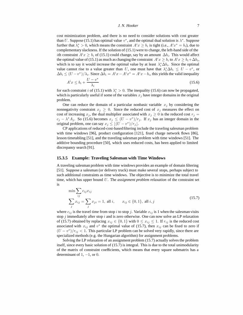
cost minimization problem, and there is no need to consider solutions with cost greaterthanU . Suppose (15.1) has optimal valuev∗, and the optimal dual solution isλ∗. Supposefurther thatλ∗

i > 0, which means the constraintAix ≥ bi is tight (i.e.,Aix∗ = bi), due tocomplementary slackness. If the solution of (15.1) were to change, the left-hand side of theith constraintAix ≥ bi of (15.1) could change, say by an amount∆bi. This would affectthe optimal value of (15.1) as much as changing the constraintAix ≥ bi to Aix ≥ bi+∆bi,which is to say it would increase the optimal value by at leastλ∗

i ∆bi. Since the optimalvalue cannot rise to a value greater thanU , one must have thatλ∗

i ∆bi ≤ U − v∗, or∆bi ≤ (U −v∗)/λi. Since∆bi = Aix−Aix∗ = Aix− bi, this yields the valid inequality

Aix ≤ bi +U − v∗

λi(15.6)

for each constrainti of (15.1) withλ∗i > 0. The inequality (15.6) can now be propagated,

which is particularly useful if some of the variablesxj have integer domains in the originalproblem.

One can reduce the domain of a particular nonbasic variablexj by considering thenonnegativity constraintxj ≥ 0. Since the reduced cost ofxj measures the effect oncost of increasingxj, the dual multiplier associated withxj ≥ 0 is the reduced costrj =cj − λ∗Aj. So (15.6) becomesxj ≤ (U − v∗)/rj. If xj has an integer domain in theoriginal problem, one can sayxj ≤ b(U − v∗)/rjc.

CP applications of reduced-cost-basedfiltering include the traveling salesman problemwith time windows [96], product configuration [121], fixed charge network flows [86],lesson timetabling [51], and the traveling salesman problem with time windows [51]. Theadditive bounding procedure [50], which uses reduced costs, has been applied to limiteddiscrepancy search [91].

15.3.5 Example: Traveling Salesman with Time Windows

A traveling salesman problem with time windows provides an example of domain filtering[51]. Suppose a salesman (or delivery truck) must make several stops, perhaps subject tosuch additional constraints as time windows. The objective is to minimize the total traveltime, which has upper boundU . Theassignment problem relaxationof the constraint setis

min∑

ij

cijxij

∑

j

xij =∑

j

xji = 1, all i, xij ∈ {0, 1}, all i, j(15.7)

wherecij is the travel time from stopi to stopj. Variablexij is 1 when the salesman visitsstopj immediately after stopi and is zero otherwise. One can now solve an LP relaxationof (15.7) obtained by replacingxij ∈ {0, 1} with 0 ≤ xij ≤ 1. If rij is the reduced costassociated withxij andv∗ the optimal value of (15.7), thenxij can be fixed to zero if(U − v∗)/rij < 1. This particular LP problem can be solved very rapidly, since there arespecialized methods (e.g. the Hungarian algorithm) for assignment problems.

Solving the LP relaxation of an assignment problem (15.7) actually solves the problemitself, since every basic solution of (15.7) is integral. This is due to the total unimodularityof the matrix of constraint coefficients, which means that every square submatrix has adeterminant of1, −1, or 0.

8 15. Operations Research Methods in Constraint Programming

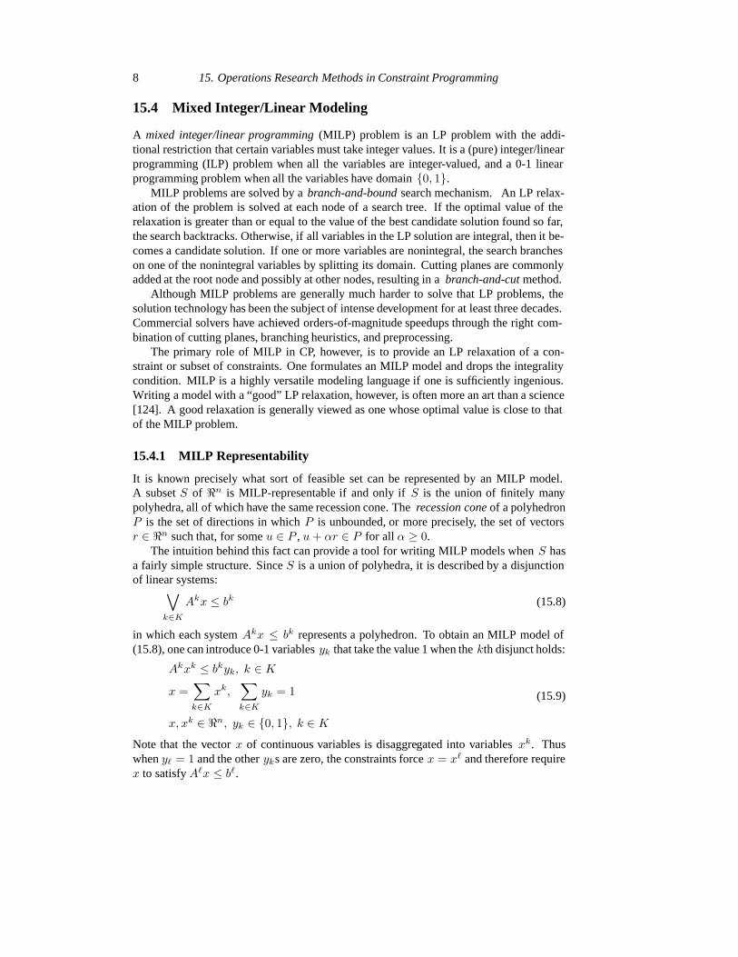
15.4 Mixed Integer/Linear Modeling

A mixed integer/linear programming(MILP) problem is an LP problem with the addi-tional restriction that certain variables must take integer values. It is a (pure) integer/linearprogramming (ILP) problem when all the variables are integer-valued, and a 0-1 linearprogramming problem when all the variables have domain{0, 1}.

MILP problems are solved by abranch-and-boundsearch mechanism. An LP relax-ation of the problem is solved at each node of a search tree. If the optimal value of therelaxation is greater than or equal to the value of the best candidate solution found so far,the search backtracks. Otherwise, if all variables in the LP solution are integral, then it be-comes a candidate solution. If one or more variables are nonintegral, the search brancheson one of the nonintegral variables by splitting its domain. Cutting planes are commonlyadded at the root node and possibly at other nodes, resulting in abranch-and-cutmethod.

Although MILP problems are generally much harder to solve that LP problems, thesolution technology has been the subject of intense development for at least three decades.Commercial solvers have achieved orders-of-magnitude speedups through the right com-bination of cutting planes, branching heuristics, and preprocessing.

The primary role of MILP in CP, however, is to provide an LP relaxation of a con-straint or subset of constraints. One formulates an MILP model and drops the integralitycondition. MILP is a highly versatile modeling language if one is sufficiently ingenious.Writing a model with a “good” LP relaxation, however, is often more an art than a science[124]. A good relaxation is generally viewed as one whose optimal value is close to thatof the MILP problem.

15.4.1 MILP Representability

It is known precisely what sort of feasible set can be represented by an MILP model.A subsetS of <n is MILP-representable if and only ifS is the union of finitely manypolyhedra, all of which have the same recession cone. Therecession coneof a polyhedronP is the set of directions in whichP is unbounded, or more precisely, the set of vectorsr ∈ <n such that, for someu ∈ P , u + αr ∈ P for all α ≥ 0.

The intuition behind this fact can provide a tool for writing MILP models whenS hasa fairly simple structure. SinceS is a union of polyhedra, it is described by a disjunctionof linear systems:

∨

k∈K

Akx ≤ bk (15.8)

in which each systemAkx ≤ bk represents a polyhedron. To obtain an MILP model of(15.8), one can introduce 0-1 variablesyk that take the value 1 when thekth disjunct holds:

Akxk ≤ bkyk, k ∈ K

x =∑

k∈K

xk,∑

k∈K

yk = 1

x, xk ∈ <n, yk ∈ {0, 1}, k ∈ K

(15.9)

Note that the vectorx of continuous variables is disaggregated into variablesxk. Thuswheny` = 1 and the otheryks are zero, the constraints forcex = x` and therefore requirex to satisfyA`x ≤ b`.

J. N. Hooker 9

.................................................................................................................................................................................................................................................................................................................................................................................................................................................................................................................................................................................................................................................................................................................

.................................................

..................................................

.................................................

..................................................

.................................................

..................................................

.................................................

..................................................

........

........

........

........

........

........

........

........

........

........

........

........

........

........

........

........

........

........

........

........

........

........

........

........

........

........

........

........

........

........

........

........

........

........

........

........

........

........

........

.

........

........

........

........

........

........

........

........

........

........

........

........

........

........

........

........

........

........

........

........

........

........

........

........

........

........

........

........

........

........

........

........

........

........

........

........

........

........

........

.

x1

x2

f..........................

.

.

.

.

.

.

.

.

.

.

.

.

.

.

.

.

.

.

.

.

.

.

.

.

.

.

.

.

.

.

.

.

.

.

.

.

.

.

.

.

.

.

.

.

.

.

.

.

.

.

.

.

.

.

.

.

.

.

.

.

.

.

.

.

.

.

.

.

.

.

.

.

.

.

.

.

.

.

.

.

.

.

.

.

.

.

.

.

.

.

.

.

.

.

.

.

.

.

.

.

.

.

.

.

.

.

.

.

.

.

.

.

.

.

.

.

.

.

.

.

.

.

.

.

.

.

.

.

.

.

.

.

.

.

.

.

.

.

.

.

.

.

.

.

.

.

.

.

.

.

.

.

.

.

.

.

.

.

.

.

.

.

.

.

.

.

.

.

.

.

.

.

.

.

.

.

.

.

.

.

.

.

.

.

.

.

.

.

.

.

.

.

.

.

.

.

.

.

.

.

.

.

.

.

.

.

.

.

.

.

.

.

.

.

.

.

.

.

.

.

.

.

.

.

.

.

.

.

.

.

.

.

.

.

.

.

.

.

.

.

.

.

.

.

.

.

.

.

.

.

.

.

.

.

.

.

.

.

.

.

.

.

.

.

.

.

.

.

.

.

.

.

.

.

.

.

.

.

.

.

.

.

.

.

.

.

.

.

.

.

.

.

.

.

.

.

.

.

.

.

.

.

.

.

.

.

.

.

.

.

.

.

.

.

.

.

.

.

.

.

.

.

.

.

.

.

.

.

.

.

.

.

.

.

.

.

.

.

.

.

.

.

.

.

.

.

.

.

.

.

.

.

.

.

.

.

.

.

.

.

.

.

.

.

.

.

.

.

.

.

.

.

.

.

.

.

.

.

.

.

.

.

.

.

.

.

.

.

.

.

.

.

.

.

.

.

.

.

.

.

.

.

.

.

.

.

.

.

.

.

.

.

.

.

.

.

.

.

.

.

.

.

.

.

.

.

.

.

.

.

.

.

.

.

.

.

.

.

.

.

.

.

.

.

.

.

.

.

.

.

.

.

.

.

.

.

.

.

.

.

.

.

.

.

.

.

.

.

.

.

.

.

.

.

.

.

.

.

.

.

.

.

.

.

.

.

.

.

.

.

.

.

.

.

.

.

.

.

.

.

.

.

.

.

.

.

.

.

.

.

.

.

.

.

.

.

.

.

.

.

.

.

.

.

.

.

.

.

.

.

.

.

.

.

.

.

.

.

.

.

.

.

.

.

.

.

.

.

.

.

.

.

.

.

.

.

.

.

.

.

.

.

.

.

.

.

.

.

.

.

.

.

.

.

.

.

.

.

.

.

.

.

.

.

.

.

.

.

.

.

.

.

.

.

.

.

.

.

.

.

.

.

.

.

.

.

.

.

.

.

.

.

.

.

.

.

.

.

.

.

.

.

.

.

.

.

.

.

.

.

.

.

.

.

.

.

.

.

.

.

.

.

.

.

.

.

.

.

.

.

.

.

.

.

.

.

.

.

.

.

.

.

.

.

.

.

.

.

.

.

.

.

.

.

.

.

.

.

.

.

.

.

.

.

.

.

.

.

.

.

.

.

.

.

.

.

.

.

.

.

.

.

.

.

.

.

.

.

.

.

.

.

.

.

.

.

.

.

.

.

.

.

.

.

.

.

.

.

.

.

.

.

.

.

.

.

.

.

.

.

.

.

.

.

.

.

.

.

.

.

.

.

.

.

.

.

.

.

.

.

.

.

.

.

.

.

.

.

.

.

.

.

.

.

.

.

.

.

.

.

.

.

.

.

.

.

.

.

.

.

.

.

.

.

.

.

.

.

.

.

.

.

.

.

.

.

.

.

.

.

.

.

.

.

.

.

.

.

.

.

.

.

.

.

.

.

.

.

.

.

.

.

.

.

.

.

.

.

.

.

.

.

.

.

.

.

.

.

.

.

.

.

.

.

.

.

.

.

.

.

.

.

.

.

.

.

.

.

.

.

.

.

.

.

.

.

.

.

.

.

.

.

.

.

.

.

.

.

.

.

.

.

.

.

.

.

.

.

.

.

.

.

.

.

.

.

.

.

.

.

.

.

.

.

.

.

.

.

.

.

.

.

.

.

.

.

.

.

.

.

.

.

.

.

.

.

.

.

.

.

.

.

.

.

.

.

.

.

.

.

.

.

.

.

.

.

.

.

.

.

.

.

.

.

.

.

.

.

.

.

.

.

.

.

.

.

.

.

.

.

.

.

.

.

.

.

.

.

.

.

.

.

.

.

.

.

.

.

.

.

.

.

.

.

.

.

.

.

.

.

.

.

.

.

.

.

.

.

.

.

.

.

.

.

.

.

.

.

.

.

.

.

.

.

.

.

.

.

.

.

.

.

.

.

.

.

.

.

.

.

.

.

.

.

.

.

.

.

.

.

.

.

.

.

.

.

.

.

.

.

.

.

.

.

.

.

.

.

.

.

.

.

.

.

.

.

.

.

.

.

.

.

.

.

.

.

.

.

.

.

.

.

.

.

.

.

.

.

.

.

.

.

.

.

.

.

.

.

.

.

.

.

.

.

.

.

.

.

.

.

.

.

.

.

.

.

.

.

.

.

.

.

.

.

.

.

.

.

.

.

.

.

.

.

.

.

.

.

.

.

.

.

.

.

.

.

.

.

.

.

.

.

.

.

.

.

.

.

.

.

.

.

.

.

.

.

.

.

.

.

.

.

.

.

.

.

.

.

.

.

.

.

.

.

.

.

.

.

.

.

.

.

.

.

.

.

.

.

.

.

.

.

.

.

.

.

.

.

.

.

.

.

.

.

.

.

.

.

.

.

.

.

.

.

.

.

.

.

.

.

.

.

.

.

.

.

.

.

.

.

.

.

.

.

.

.

.

.

.

.

.

.

.

.

.

.

.

.

.

.

.

.

.

.

.

.

.

.

.

.

.

.

.

.

.

.

.

.

.

.

.

.

.

.

.

.

.

.

.

.

.

.

.

.

.

.

.

.

.

.

.

.

.

.

.

.

.

.

.

.

.

.

.

.

.

.

.

.

.

.

.

.

.

.

.

.

.

.

.

.

.

.

.

.

.

.

.

.

.

.

.

.

.

.

.

.

.

.

.

.

.

.

.

.

.

.

.

.

.

.

.

.

.

.

.

.

.

.

.

.

.

.

.

.

.

.

.

.

.

.

.

.

.

.

.

.

.

.

.

.

.

.

.

.

.

.

.

.

.

.

.

.

.

.

.

.

.

.

.

.

.

.

.

.

.

.

.

.

.

.

.

.

.

.

.

.

.

.

.

.

.

.

.

.

.

.

.

.

.

.

.

.

.

.

.

.

.

.

.

.

.

.

.

.

.

.

.

.

.

.

.

.

.

.

.

.

.

.

.

.

.

.

.

.

.

.

.

.

.

.

.

.

.

.

.

.

.

.

.

.

.

.

.

.

.

.

.

.

.

.

.

.

.

.

.

.

.

.

.

.

.

.

.

.

.

.

.

.

.

.

.

.

.

.

.

.

.

.

.

.

.

.

.

.

.

.

.

.

.

.

.

.

.

.

.

.

.

.

.

.

.

.

.

.

.

.

.

.

.

.

.

.

.

.

.

.

.

.

.

.

.

.

.

.

.

.

.

.

.

.

.

.

.

.

.

.

.

.

.

.

.

.

.

.

.

.

.

.

.

.

.

.

.

.

.

.

.

.

.

.

.

.

.

.

.

.

.

.

.

.

.

.

.

.

.

.

.

.

.

.

.

.

.

.

.

.

.

.

.

.

.

.

.

.

.

.

.

.

.

.

.

.

.

.

.

.

.

.

.

.

.

.

.

.

.

.

.

.

.

.

.

.

.

.

.

.

.

.

.

.

.

.

.

.

.

.

.

.

.

.

.

.

.

.

.

.

.

.

.

.

.

.

.

.

.

.

.

.

.

.

.

.

.

(i)

........

........

........

........

........

........

........

........

........

........

........

........

........

........

........

........

........

........

........

........

........

........

........

.......................

...................

Recessioncone of P1

........

........

........

........

........

........

........

........

........

........

........

........

........

........

........

........

........

........

........

........

........

........

........

.......................

...................

.................................................

..................................................

.................................................

.....................................................................

...................

Recessioncone of P2

.................................................................................................................................................................................................................................................................................................................................................................................................................................................................................................................................................................................................................................................................................................................

.................................................

..................................................

.................................................

..................................................

.................................................

..................................................

.................................................

..................................................

........

........

........

........

........

........

........

........

........

........

........

........

........

........

........

........

........

........

........

........

........

........

........

........

........

........

........

........

........

........

........

........

........

........

........

........

........

........

........

.

........

........

........

........

........

........

........

........

........

........

........

........

........

........

........

........

........

........

........

........

........

........

........

........

........

........

........

........

........

........

........

........

........

........

........

........

........

........

........

.

........

........

........

........

........

........

........

........

........

........

........

........

........

........

........

........

........

........

........

........

........

........

........

........

........

........

........

........

........

........

........

........

........

........

........

........

........

........

........

.

x1

x2

f

M

.

.

.

.

.

.

.

.

.

.

.

.

.

.

.

.

.

.

.

.

.

.

.

.

.

.

.

.

.

.

.

.

.

.

.

.

.

.

.

.

.

.

.

.

.

.

.

.

.

.

.

.

.

.

.

.

.

.

.

.

.

.

.

.

.

.

.

.

.

.

.

.

.

.

.

.

.

.

.

.

.

.

.

.

.

.

.

.

.

.

.

.

.

.

.

.

.

.

.

.

.

.

.

.

.

.

.

.

.

.

.

.

.

.

.

.

.

.

.

.

.

.

.

.

.

.

.

.

.

.

.

.

.

.

.

.

.

.

.

.

.

.

.

.

.

.

.

.

.

.

.

.

.

.

.

.

.

.

.

.

.

.

.

.

.

.

.

.

.

.

.

.

.

.

.

.

.

.

.

.

.

.

.

.

.

.

.

.

.

.

.

.

.

.

.

.

.

.

.

.

.

.

.

.

.

.

.

.

.

.

.

.

.

.

.

.

.

.

.

.

.

.

.

.

.

.

.

.

.

.

.

.

.

.

.

.

.

.

.

.

.

.

.

.

.

.

.

.

.

.

.

.

.

.

.

.

.

.

.

.

.

.

.

.

.

.

.

.

.

.

.

.

.

.

.

.

.

.

.

.

.

.

.

.

.

.

.

.

.

.

.

.

.

.

.

.

.

.

.

.

.

.

.

.

.

.

.

.

.

.

.

.

.

.

.

.

.

.

.

.

.

.

.

.

.

.

.

.

.

.

.

.

.

.

.

.

.

.

.

.

.

.

.

.

.

.

.

.

.

.

.

.

.

.

.

.

.

.

.

.

.

.

.

.

.

.

.

.

.

.

.

.

.

.

.

.

.

.

.

.

.

.

.

.

.

.

.

.

.

.

.

.

.

.

.

.

.

.

.

.

.

.

.

.

.

.

.

.

.

.

.

.

.

.

.

.

.

.

.

.

.

.

.

.

.

.

.

.

.

.

.

.

.

.

.

.

.

.

.

.

.

.

.

.

.

.

.

.

.

.

.

.

.

.

.

.

.

.

.

.

.

.

.

.

.

.

.

.

.

.

.

.

.

.

.

.

.

.

.

.

.

.

.

.

.

.

.

.

.

.

.

.

.

.

.

.

.

.

.

.

.

.

.

.

.

.

.

.

.

.

.

.

.

.

.

.

.

.

.

.

.

.

.

.

.

.

.

.

.

.

.

.

.

.

.

.

.

.

.

.

.

.

.

.

.

.

.

.

.

.

.

.

.

.

.

.

.

.

.

.

.

.

.

.

.

.

.

.

.

.

.

.

.

.

.

.

.

.

.

.

.

.

.

.

.

.

.

.

.

.

.

.

.

.

.

.

.

.

.

.

.

.

.

.

.

.

.

.

.

.

.

.

.

.

.

.

.

.

.

.

.

.

.

.

.

.

.

.

.

.

.

.

.

.

.

.

.

.

.

.

.

.

.

.

.

.

.

.

.

.

.

.

.

.

.

.

.

.

.

.

.

.

.

.

.

.

.

.

.

.

.

.

.

.

.

.

.

.

.

.

.

.

.

.

.

.

.

.

.

.

.

.

.

.

.

.

.

.

.

.

.

.

.

.

.

.

.

.

.

.

.

.

.

.

.

.

.

.

.

.

.

.

.

.

.

.

.

.

.

.

.

.

.

.

.

.

.

.

.

.

.

.

.

.

.

.

.

.

.

.

.

.

.

.

.

.

.

.

.

.

.

.

.

.

.

.

.

.

.

.

.

.

.

.

.

.

.

.

.

.

.

.

.

.

.

.

.

.

.

.

.

.

.

.

.

.

.

.

.

.

.

.

.

.

.

.

.

.

.

.

.

.

.

.

.

.

.

.

.

.

.

.

.

.

.

.

.

.

.

.

.

.

.

.

.

.

.

.

.

.

.

.

.

.

.

.

.

.

.

.

.

.

.

.

.

.

.

.

.

.

.

.

.

.

.

.

.

.

.

.

.

.

.

.

.

.

.

.

.

.

.

.

.

.

.

.

.

.

.

.

.

.

.

.

.

.

.

.

.

.

.

.

.

.

.

.

.

.

.

.

.

.

.

.

.

.

.

.

.

.

.

.

.

.

.

.

.

.

.

.

.

.

.

.

.

.

.

.

.

.

.

.

.

.

.

.

.

.

.

.

.

.

.

.

.

.

.

.

.

.

.

.

.

.

.

.

.

.

.

.

.

.

.

.

.

.

.

.

.

.

.

.

.

.

.

.

.

.

.

.

.

.

.

.

.

.

.

.

.

.

.

.

.

.

.

.

.

.

.

.

.

.

.

.

.

.

.

.

.

.

.

.

.

.

.

.

.

.

.

.

.

.

.

.

.

.

.

.

.

.

.

.

.

.

.

.

.

.

.

.

.

.

.

.

.

.

.

.

.

.

.

.

.

.

.

.

.

.

.

.

.

.

.

.

.

.

.

.

.

.

.

.

.

.

.

.

.

.

.

.

.

.

.

.

.

.

.

.

.

.

.

.

.

.

.

.

.

.

.

.

.

.

.

.

.

.

.

.

.

.

.

.

.

.

.

.

.

.

.

.

.

.

.

.

.

.

.

.

.

.

.

.

.

.

.

.

.

.

.

.

.

.

.

.

.

.

.

.

.

.

.

.

.

.

.

.

.

.

.

.

.

.

.

.

.

.

.

.

.

.

.

.

.

.

.

.

.

.

.

.

.

.

.

.

.

.

.

.

.

.

.

.

.

.

.

.

.

.

.

.

.

.

.

.

.

.

.

.

.

.

.

.

.

.

.

.

.

.

.

.

.

.

.

.

.

.

.

.

.

.

.

.

.

.

.

.

.

.

.

.

.

.

.

.

.

.

.

.

.

.

.

.

.

.

.

.

.

.

.

.

.

.

.

.

.

.

.

.

.

.

.

.

.

.

.

.

.

.

.

.

.

.

.

.

.

.

.

.

.

.

.

.

.

.

.

.

.

.

.

.

.

.

.

.

.

.

(ii)

........

........

........

........

........

........

........

........

........

........

........

........

........

........

........

........

........

........

........

........

........

........

........

.......................

...................

Recessioncone of P1, P2

1

Figure 15.1:(i) Feasible set of a fixed charge problem, consisting of the union of polyhedraP1 (heavy line) andP2 (shaded area). (ii) Feasible set of the same problem with the boundx1 ≤ M , whereP ′

2 is the shaded area.

There are a number of devices for writing MILP formulations when (15.10) does notyield a practical model. A comprehensive discussion of these may be found in [127].

15.4.2 Example: Fixed Charge Function

MILP representability is illustrated by the fixed charge function, which occurs frequentlyin modeling. Suppose the costx2 of producing quantityx1 is bounded below by zero whenthe production quantityx1 is zero, andf + cx1 otherwise, wheref is the fixed cost andcthe unit variable cost. IfS is the set of feasible points(x1, x2), thenS is the union of twopolyhedraP1 andP2 (Fig 15.1a). The recession cone ofP1 is P1 itself, and the recessioncone ofP2 is the set of all vectors(x1, x2) with x2 ≥ cx1 ≥ 0. Since these cones are notidentical,S is not MILP-representable.

However, in practice one can put a sufficiently large upper boundM on x1. Now therecession cone of each of the resulting polyhedraP1, P

′2 (Fig. 15.1b) is the same (namely,

P1), and the feasible setS′ = P1 ∪ P ′2 is therefore MILP-representable.P1 is the poly-

hedron described byx1 ≤ 0, x1, x2 ≥ 0, andP ′2 is described bycx1 − x2 ≤ −f, x1 ≤

10 15. Operations Research Methods in Constraint Programming

M, x1 ≥ 0. So (15.9) becomes

x11 ≤ 0

x11, x

22 ≥ 0

cx21 − x2

2 ≤ −fy2

0 ≤ x1 ≤ My2

x1 = x11 + x2

1

x2 = x12 + x2

2

y1 + y2 = 1

y1, y2 ∈ {0, 1}(15.10)

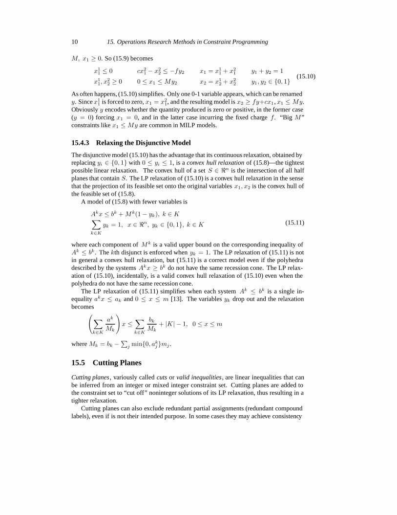
As often happens, (15.10) simplifies. Only one 0-1 variable appears, which can be renamedy. Sincex1

1 is forced to zero,x1 = x21, and the resulting model isx2 ≥ fy+cx1, x1 ≤ My.

Obviouslyy encodes whether the quantity produced is zero or positive, in the former case(y = 0) forcing x1 = 0, and in the latter case incurring the fixed chargef . “Big M ”constraints likex1 ≤ My are common in MILP models.

15.4.3 Relaxing the Disjunctive Model

The disjunctive model (15.10) has the advantage that its continuous relaxation, obtained byreplacingyi ∈ {0, 1} with 0 ≤ yi ≤ 1, is aconvex hull relaxationof (15.8)—the tightestpossible linear relaxation. The convex hull of a setS ∈ <n is the intersection of all halfplanes that containS. The LP relaxation of (15.10) is a convex hull relaxation in the sensethat the projection of its feasible set onto the original variablesx1, x2 is the convex hull ofthe feasible set of (15.8).

A model of (15.8) with fewer variables is

Akx ≤ bk + Mk(1 − yk), k ∈ K∑

k∈K

yk = 1, x ∈ <n, yk ∈ {0, 1}, k ∈ K (15.11)

where each component ofMk is a valid upper bound on the corresponding inequality ofAk ≤ bk. Thekth disjunct is enforced whenyk = 1. The LP relaxation of (15.11) is notin general a convex hull relaxation, but (15.11) is a correct model even if the polyhedradescribed by the systemsAkx ≥ bk do not have the same recession cone. The LP relax-ation of (15.10), incidentally, is a valid convex hull relaxation of (15.10) even when thepolyhedra do not have the same recession cone.

The LP relaxation of (15.11) simplifies when each systemAk ≤ bk is a single in-equalityakx ≤ ak and0 ≤ x ≤ m [13]. The variablesyk drop out and the relaxationbecomes

(∑

k∈K

ak

Mk

)x ≤

∑

k∈K

bk

Mk+ |K| − 1, 0 ≤ x ≤ m

whereMk = bk −∑

j min{0, akj}mj .

15.5 Cutting Planes

Cutting planes, variously calledcutsor valid inequalities, are linear inequalities that canbe inferred from an integer or mixed integer constraint set. Cutting planes are added tothe constraint set to “cut off” noninteger solutions of its LP relaxation, thus resulting in atighter relaxation.

Cutting planes can also exclude redundant partial assignments (redundant compoundlabels), even if is not their intended purpose. In some cases they may achieve consistency

J. N. Hooker 11

.....................................................................................................................................................................................................................................................................................................................................................................................................................................................................................................................................................................................................................................................................................................

x1

x2

..........................................................................................................................................................................................................................................................................................................................................................................................................................................•

•

•

•

•

.................................

.

.

.

.

.

.

.

.

.

.

.

.

.

.

.

.

.

.

.

.

.

.

.

.

.

.

.

.

.

.

.

.

.

.

.

.

.

.

.

.

.

.

.

.

.

.

.

.

.

.

.

.

.

.

.

.

.

.

.

.

.

.

.

.

.

.

.

.

.

.

.

.

.

.

.

.

.

.

.

.

.

.

.

.

.

.

.

.

.

.

.

.

.

.

.

.

.

.

.

.

.

.

.

.

.

.

.

.

.

.

.

.

.

.

.

.

.

.

.

.

.

.

.

.

.

.

.

.

.

.

.

.

.

.

.

.

.

.

.

.

.

.

.

.

.

.

.

.

.

.

.

.

.

.

.

.

.

.

.

.

.

.

.

.

.

.

.

.

.

.

.

.

.

.

.

.

.

.

.

.

.

.

.

.

.

.

.

.

.

.

.

.

.

.

.

.

.

.

.

.

.

.

.

.

.

.

.

.

.

.

.

.

.

.

.

.

.

.

.

.

.

.

.

.

.

.

.

.

.

.

.

.

.

.

.

.

.

.

.

.

.

.

.

.

.

.

.

.

.

.

.

.

.

.

.

.

.

.

.

.

.

.

.

.

.

.

.

.

.

.

.

.

.

.

.

.

.

.

.

.

.

.

.

.

.

.

.

.

.

.

.

.

.

.

.

.

.

.

.

.

.

.

.

.

.

.

.

.

.

.

.

.

.

.

.

.

.

.

.

.

.

.

.

.

.

.

.

.

.

.

.

.

.

.

.

.

.

.

.

.

.

.

.

.

.

.

.

.

.

.

.

.

.

.

.

.

.

.

.

.

.

.

.

.

.

.

.

.

.

.

.

.

.

.

.

.

.

.

.

.

.

.

.

.

.

.

.

.

.

.

.

.

.

.

.

.

.

.

.

.

.

.

.

.

.

.

.

.

.

.

.

.

.

.

.

.

.

.

.

.

.

.

.

.

.

.

.

.

.

.

.

.

.

.

.

.

.

.

.

.

.

.

.

.

.

.

.

.

.

.

.

.

.

.

.

.

.

.

.

.

.

.

.

.

.

.

.

.

.

.

.

.

.

.

.

.

.

.

.

.

.

.

.

.

.

.

.

.

.

.

.

.

.

.

.

.

.

.

.

.

.

.

.

.

.

.

.

.

.

.

.

.

.

.

.

.

.

.

.

.

.

.

.

.

.

.

.

.

.

.

.

.

.

.

.

.

.

.

.

.

.

.

.

.

.

.

.

.

.

.

.

.

.

.

.

.

.

.

.

.

.

.

.

.

.

.

.

.

.

.

.

.

.

.

.

.

.

.

.

.

.

.

.

.

.

.

.

.

.

.

.

.

.

.

.

.

.

.

.

.

.

.

.

.

.

.

.

.

.

.

.

.

.

.

.

.

.

.

.

.

.

.

.

.

.

.

.

.

.

.

.

.

.

.

.

.

.

.

.

.

.

.

.

.

.

.

.

.

.

.

.

.

.

.

.

.

.

.

.

.

.

.

.

.

.

.

.

.

.

.

.

.

.

.

.

.

.

.

.

.

.

.

.

.

.

.

.

.

.

.

.

.

.

.

.

.

.

.

.

.

.

.

.

.

.

.

.

.

.

.

.

.

.

.

.

.

.

.

.

.

.

.

.

.

.

.

.

.

.

.

.

.

.

.

.

.

.

.

.

.

.

.

.

.

.

.

.

.

.

.

.

.

.

.

.

.

.

.

.

.

.

.

.

.

.

.

.

.

.

.

.

.

.

.

.

.

.

.

.

.

.

.

.

.

.

.

.

.

.

.

.

.

.

.

.

.

.

.

.

.

.

.

.

.

.

.

.

.

.

.

.

.

.

.

.

.

.

.

.

.

.

.

.

.

.

.

.

.

.

.

.

.

.

.

.

.

.

.

.

.

.

.

.

.

.

.

.

.

.

.

.

.

.

.

.

.

.

.

.

.

.

.

.

.

.

.

.

.

.

.

.

.

.

.

.

.

.

.

.

.

.

.

.

.

.

.

.

.

.

.

.

.

.

.

.

.

.

.

.

.

.

.

.

.

.

.

.

.

.

.

.

.

.

.

.

.

.

.

.

.

.

.

.

.

.

.

.

.

.

.

.

.

.

.

.

.

.

.

.

.

.

.

.

.

.

.

.

.

.

.

.

.

.

.

.

.

.

.

.

.

.

.

.

.

.

.

.

.

.

.

.

.

.

.

.

.

.

.

.

.

.

.

.

.

.

.

.

.

.

.

.

.

.

.

.

.

.

.

.

.

.

.

.

.

.

.

.

.

.

.

.

.

.

.

.

.

.

.

.

.

.

.

.

.

.

.

.

.

.

.

.

.

.

.

.

.

.

.

.

.

.

.

.

.

.

.

.

.

.

.

.

.

.

.

.

.

.

.

.

.

.

.

.

.

.

.

.

.

.

.

.

.

.

.

.

.

.

.

.

.

.

.

.

.

.

.

.

.

.

.

.

.

.

.

.

.

.

.

.

.

.

.

.

.

.

.

.

.

.

.

.

.

.

.

.

.

.

.

.

.

.

.

.

.

.

.

.

.

.

.

.

.

.

.

.

.

.

.

.

.

.

.

.

.

.

.

.

.

.

.

.

.

.

.

.

.

.

....

........

.....

........

.....

........

.....

........

.....

........

.....

........

.....

........

.....

........

.....

........

.....

........

.....

........

.....

........

.....

........

.....

........

.....

........

.....

........

.....

........

.....

........

.....

........

.....

........

.....

........

.....

........

.....

........

.....

........

.....

........

.....

........

.....

........

.....

........

.....

1

Figure 15.2:Feasible set (shaded area) of the LP relaxation of a systemx1 + x2 ≤ 2,x1 − x2 ≤ 0 with domainsxj ∈ {0, 1, 2}, and a cutting planex1 ≤ 1 (dashed line).

of one kind or another, even though the concept of consistency never developed in the ORcommunity. It is therefore likely that cutting planes reduce backtracking in branch-and-bound algorithms by excluding redundant partial assignments, quite apart from their rolein strengthening relaxations.

For example,x1 ≤ 1 is a cutting plane for the systemx1 + x2 ≤ 2, x1 − x2 ≤ 1 inwhich eachxj has domain{0, 1, 2}. As Fig. 15.2 shows,x1 ≤ 1 is valid because it cutsoff no feasible (0-1) points. Yet it cuts off part of the feasible set of the LP relaxationand therefore strengthens the LP relaxation, in fact resulting in a convex hull relaxation.Adding the cut also achieves arc consistency for the constraint set, since it reducesx1’sdomain to{0, 1}.

A few basic types of cutting planes are surveyed here. General references on cut-ting planes include [93, 99, 130], and the role of cutting planes in CP is further dis-cussed in [20, 22, 38, 52, 69, 77]. CP-based application of cutting planes include theorthogonal Latin squares problem [6], truss structure design [23], processing networkdesign [60, 77], single-vehicle routing [110], resource-constrained scheduling [40], multi-ple machine scheduling [22], boat party scheduling [77], and the multidimensional knap-sack problem [100]. Cutting planes for disjunctions of linear systems have been applied tofactory retrofit planning, strip packing, and zero-wait job shop scheduling [111].

15.5.1 Chvatal-Gomory Cuts

One can always generate a cutting plane for an integer linear systemAx ≤ b by taking anonnegative linear combinationuAx ≤ ub of the inequalities in the system and roundingdown all fractions that result. This yields the cutbuAcx ≤ bubc, whereu ≥ 0. Forexample, one can obtain the cutx1 ≤ 0 from x1 + x2 ≤ 1 andx1 − x2 ≤ 0 (Fig. 15.2) bygiving each a multiplier of12 in the linear combination.

12 15. Operations Research Methods in Constraint Programming

After generating a cut of this kind, one can add it toAx ≤ b and repeat the process.Any cut generated recursively in this fashion is aChvatal-Gomory cut. A fundamentalresult of cutting plane theory is that every cut is a Chv´atal-Gomory cut [31].

A subset of Chv´atal-Gomory cuts are enough to achieve consistency. If two particulartypes of cuts,resolventsanddiagonal sums, are recursively derived from 0-1 inequalitiesthat are dominated by inequalities inAx ≤ b, then every inequality implied byAx ≤ b(up to equivalence) is implied by one of the generated cuts; see [67, 70] for details. Thisfact leads to a logic-based method for 0-1 linear constraint solving [12]. The derivation ofresolvents alone is enough to achieve strongn-consistency and therefore hyperarc consis-tency.

15.5.2 General Separating Cuts

Since it is impractical to generate all Chv´atal-Gomory cuts, a more common approach isto identify one or more cuts that exclude or “cut off” a nonintegral solution of the currentLP relaxation. These are known asseparating cutsbecause they separate the nonintegralsolution from the convex hull of the original problem’s feasible set. For instance, if the LPrelaxation of the example in Fig. 15.2 has the solution(3

2 , 12), thenx1 ≤ 1 is a separating

cut.A general-purpose separating cut can be generated by solving the LP relaxation of an

integer system in equality form (15.2) to obtain a basic solution(b, 0), whereb = B−1b.If xi is any basic variable with a nonintegral value in this solution, the valid inequality

xi ≤ bbic − bNicxN (15.12)

cuts off (b, 0). HereN = B−1N , andNi refers to theith row of N . This cut is popularlyknown as aGomory cut.

For many years Gomory cuts were believed to be ineffective, but now it is known thatthey can be very useful if sufficiently many are generated. Multiple cuts can be obtainedby generating one for each nonintegralxi, or perhaps by re-solving the LP with cuts addedand generating further Gomory cuts.

Gomory cuts have an analog for MILP systems, known asseparating mixed integerrounding cuts[94], that are equally important in practice. Let the MILP system in equalityform beA1y + A2x = b with x, y ≥ 0 andy integer. LetB andN be basic and nonbasiccolumns in the LP relaxation as before, and suppose that a basic variableyi is nonintegral.DefineJ to be the set of indicesj for which yj is basic andK to be the set of indicesfor which xj is basic. Also letJ1 = {j ∈ J | frac(Nij) ≥ frac(bi)} andJ2 = J \ J1,where frac(α) = α− bαc is the fractional part ofα. Then the following is a mixed integerrounding cut that cuts off the nonintegral solution:

yi ≥ bbic −∑

j∈J1

dNijeyj −∑

j∈J2

(bNikc +

frac(Nij)frac(bi)

)yj −

1frac(bi)

∑

j∈K

N+ij xj

whereN+ij = max{0, Nij}.

15.5.3 Knapsack Cuts

Knapsack cuts, also known aslifted covering inequalities, are defined for an integer linearinequalityax ≤ α with a ≥ 0. (One can always obtaina ≥ 0 by replacing eachxj that

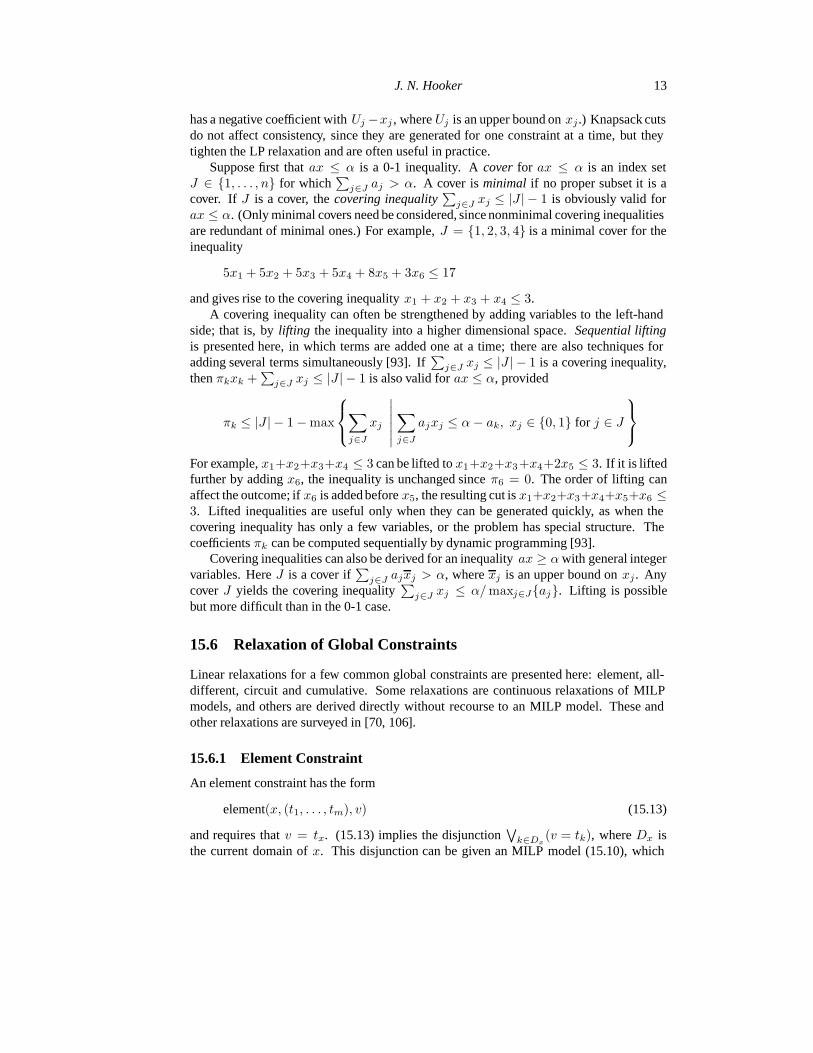
J. N. Hooker 13

has a negative coefficient withUj −xj , whereUj is an upper bound onxj.) Knapsack cutsdo not affect consistency, since they are generated for one constraint at a time, but theytighten the LP relaxation and are often useful in practice.

Suppose first thatax ≤ α is a 0-1 inequality. Acover for ax ≤ α is an index setJ ∈ {1, . . . , n} for which

∑j∈J aj > α. A cover isminimal if no proper subset it is a

cover. If J is a cover, thecovering inequality∑

j∈J xj ≤ |J | − 1 is obviously valid forax ≤ α. (Only minimal covers need be considered, since nonminimal covering inequalitiesare redundant of minimal ones.) For example,J = {1, 2, 3, 4} is a minimal cover for theinequality

5x1 + 5x2 + 5x3 + 5x4 + 8x5 + 3x6 ≤ 17

and gives rise to the covering inequalityx1 + x2 + x3 + x4 ≤ 3.A covering inequality can often be strengthened by adding variables to the left-hand

side; that is, bylifting the inequality into a higher dimensional space.Sequential liftingis presented here, in which terms are added one at a time; there are also techniques foradding several terms simultaneously [93]. If

∑j∈J xj ≤ |J | − 1 is a covering inequality,

thenπkxk +∑

j∈J xj ≤ |J | − 1 is also valid forax ≤ α, provided

πk ≤ |J | − 1 − max

∑

j∈J

xj

∣∣∣∣∣∣∑

j∈J

ajxj ≤ α − ak, xj ∈ {0, 1} for j ∈ J

For example,x1+x2+x3+x4 ≤ 3 can be lifted tox1+x2+x3+x4+2x5 ≤ 3. If it is liftedfurther by addingx6, the inequality is unchanged sinceπ6 = 0. The order of lifting canaffect the outcome; ifx6 is added beforex5, the resulting cut isx1+x2+x3+x4+x5+x6 ≤3. Lifted inequalities are useful only when they can be generated quickly, as when thecovering inequality has only a few variables, or the problem has special structure. Thecoefficientsπk can be computed sequentially by dynamic programming [93].

Covering inequalities can also be derived for an inequalityax ≥ α with general integervariables. HereJ is a cover if

∑j∈J ajxj > α, wherexj is an upper bound onxj. Any

coverJ yields the covering inequality∑

j∈J xj ≤ α/ maxj∈J{aj}. Lifting is possiblebut more difficult than in the 0-1 case.

15.6 Relaxation of Global Constraints

Linear relaxations for a few common global constraints are presented here: element, all-different, circuit and cumulative. Some relaxations are continuous relaxations of MILPmodels, and others are derived directly without recourse to an MILP model. These andother relaxations are surveyed in [70, 106].

15.6.1 Element Constraint

An element constraint has the form

element(x, (t1, . . . , tm), v) (15.13)

and requires thatv = tx. (15.13) implies the disjunction∨

k∈Dx(v = tk), whereDx is

the current domain ofx. This disjunction can be given an MILP model (15.10), which

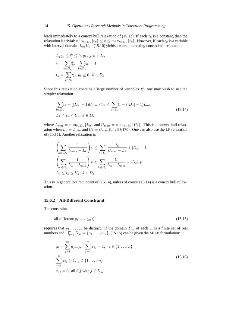
14 15. Operations Research Methods in Constraint Programming

leads immediately to a convex hull relaxation of (15.13). If eachtk is a constant, then therelaxation is trivial:mink∈Dx{tk} ≤ v ≤ maxk∈Dx{tk}. However, if eachtk is a variablewith interval domain[Lk, Uk], (15.10) yields a more interesting convex hull relaxation:

Ljyk ≤ tkj ≤ Ujyk, j, k ∈ Dx

v =∑

k∈Dx

tkk,∑

k∈Dx

yk = 1

tk =∑

j∈Dx

tjk, yk ≥ 0, k ∈ Dx

Since this relaxation contains a large number of variablestki , one may wish to use thesimpler relaxation

∑

k∈Dx

tk − (|Dx| − 1)Umax ≤ v ≤∑

k∈Dx

tk − (|Dx| − 1)Lmin

Lk ≤ tk ≤ Uk, k ∈ Dx

(15.14)

whereLmin = mink∈Dx{Lk} andUmax = maxk∈Dx{Uk}. This is a convex hull relax-ation whenLk = Lmin andUk = Umax for all k [70]. One can also use the LP relaxationof (15.11). Another relaxation is

(∑

k∈Dx

1Umax − Lk

)v ≤

∑

k∈Dx

tkUmax − Lk

+ |Dx| − 1

(∑

k∈Dx

1Uk − Lmin

)v ≥

∑

k∈Dx

tkUk − Lmin

− |Dx|+ 1

Lk ≤ tk ≤ Uk, k ∈ Dx

This is in general not redundant of (15.14), unless of course (15.14) is a convex hull relax-ation.

15.6.2 All-Different Constraint

The constraint

all-different(y1, . . . , yn)) (15.15)

requires thaty1, . . . , yn be distinct. If the domainDyi of eachyi is a finite set of realnumbers and

⋃ni=1 Dyi = {a1, . . . , am}, (15.15) can be given the MILP formulation:

yi =m∑

j=1

ajxij,

m∑

j=1

xij = 1, i ∈ {1, . . . , n}

n∑

i=1

xij ≥ 1, j ∈ {1, . . . , m}

xij = 0, all i, j with j 6∈ Dyi

(15.16)

J. N. Hooker 15

where the binary variablexij = 1 whenyi = j. A continuous relaxation can be obtainedby replacingxij ∈ {0, 1} with xij ≥ 0. This is a convex hull relaxation, in the sense thatthe projection of its feasible set onto the variablesyi is the convex hull of the feasible setof (15.15).

The MILP formulation (15.16) is convenient for some problems and not for others.Suppose for instance the problem is to find a minimum-cost assignment of jobs to workers,wherecij is the cost of assigning jobj to workeri. The constraint (15.15) requires thatevery worker get a different job, and the problem is to minimize

∑ni=1 ciyi subject to

(15.15). MILP solves the problem by minimizing∑

ij cijxij subject to (15.16).However, if one wishes to find a minimum-cost route in a traveling salesman problem,

the objective function becomes nonlinear in the integer model. (15.15) is a correct modelfor this problem only ifyi is theith stop visited, rather than the stop visited immediatelyafteri as in (15.7). So ifcij is the travel time fromi to j as before, the problem is to mini-mize

∑ni=1 cyiyi+1 subject to (15.15), whereyn+1 is identified withy1. The integer model

must minimize the nonlinear expression∑

ijk cjkxijxi+1,k subject to (15.16). However,there are linear 0-1 models for this problem, the most popular of which is presented in thenext section.

If Dyi is the same set of numbers{a1, . . . , am} for eachi, with a1 ≤ · · · ≤ am, aconvex hull relaxation [70, 75, 128] can be written in the original variables:

|J |∑

j=1

aj ≤∑

j∈J

xj ≤m∑

j=m−|J |+1

aj, all J ⊂ {1, . . . , n}

There are exponentially many constraints, but one can start by using only the constraints

n∑

j=1

aj ≤n∑

j=1

xj ≤m∑

j=m−n+1

aj

and bounds on the variables, and then generate separating cuts as needed. Letx bethe solution of the current relaxation of the problem, and renumber the variables so thatx1 ≤ · · · ≤ xn. Then for eachi = 2, . . . , n− 1 one can generate the cut

i∑

j=1

xj ≥i∑

j=1

aj

if∑i

j=1 xj <∑i

j=1 aj. Also for eachi = n − 1, . . . , 2 generate the cut

n∑

j=i

xj ≤m∑

j=m−n+i

aj

if∑n

j=i xj >∑m

j=m−n+i aj. There is no separating cut ifx lies within the convex hull ofthe alldiff feasible set.

Relaxation of multiple all-different constraints is discussed in [5] and of two overlap-ping all-different constraints in [34].

16 15. Operations Research Methods in Constraint Programming

15.6.3 Circuit Constraint

The constraint

circuit(y1, . . . , yn) (15.17)

requires thatz1, . . . , zn be a permutation of1, . . . , n, where eachzi = yzi−1 (andz0 isidentified withzn). The domainDyi of eachyi is a subset of{1, . . . , n}. The elements1, . . . , n may be viewed as vertices of a directed graphG that contains an edge(i, j)wheneverj ∈ Dyi . An edge(i, j) is selected whenyi = j, and (15.17) requires that theselected edges form a hamiltonian circuit.

The circuit constraint can be modeled with a traveling salesman formulation. Let the0-1 variablexij (for i 6= j) take the value 1 whenyi = j:

n∑

j=1

xij =n∑

j=1

xji = 1, i ∈ {1, . . . , n} (a)

∑

(i,j)∈δ(S)

xij ≥ 1, all S ⊂ {1, . . . , n} with 2 ≤ |S| ≤ n − 2 (b)(15.18)

Hereδ(S) is the set of edges(i, j) of G for which i ∈ S andj 6∈ S. If j 6∈ Dyi , theformulation (15.18) omits variablexij. Constraints (a) comprise the assignment relaxation(15.7) already discussed. Thesubtour elimination constraints(b) exclude circuits withinproper subsetsS of {1, . . . , n} by requiring that at least one edge connect a vertex inS toone outsideS.

The traveling salesmanproblem minimizes∑

i cixi subject to (15.17). Its MILP formu-lation minimizes

∑ij cijxij subject to (15.18) andxij ∈ {0, 1}. There are exponentially

many subtour elimination constraints in this formulation, but one can begin with a relax-ation of the problem (such as the assignment relaxation) and add separating cuts as needed.If x is a solution of the current relaxation, let thecapacityof edge(i, j) be xij. Select aproper subsetS of the vertices for which the total capacity of edges leavingS is a mini-mum. The subtour elimination constraint (15.18b) corresponding toS is a separating cutif the minimum capacity is less than 1. There are fast algorithms for findingS ([49, 103]).

If j ∈ Dyi if and only if i ∈ Dyj , andcij = cji, for every pairi, j, the problembecomes thesymmetrictraveling salesman problem and can be given a somewhat morecompact model that uses a2-matchingrelaxation. The OR literature has developed differ-ent (albeit related) analyses and algorithms for the symmetric and asymmetric problems;see [61] for a comprehensive discussion.

Several families of cutting planes have been developed to strengthen the LP relaxation.By far the most widely used arecomb inequalities. SupposeH is a subset of vertices ofG, andT1, . . . , Tm are pairwise disjoint sets of vertices (wherem is odd), such thatH∩Tk

andTk \ H are nonempty for eachk. H is thehandleof the comb and eachTi is a tooth.Then the following is a comb inequality for the asymmetric problem:

∑

(i,j)∈δ(H)

xij +m∑

k=1

∑

(i,j)∈δ(Tk)

xij ≥ 12(3m + 1)

One can get some intuition as to why the cut is valid by considering a comb with threeteeth and six vertices. Various proofs of validity are given in [97]. The comb inequalitiesare facet-defining whenG is a complete graph.

J. N. Hooker 17

15.6.4 Cumulative Constraint

The fundamental constraint for cumulative scheduling is

cumulative(s, p, c, C) (15.19)

where variabless = (s1, . . . , sn) represent the start times of jobs1, . . . , n. Parametersp = (p1, . . . , pn) are the processing times andc = (c1, . . . , cn) the resource consumptionrates. Release times and deadlines are implicit in the domains[Rj, Dj] of the variablessj .The constraint (15.19) requires that the total resource consumption rate at any time be lessthan or equal toC. That is,

∑j∈Jt

cj ≤ C for all t, whereJt = {j | sj ≤ t < sj + pj}.The most straightforward MILP model discretizes time and introduces a 0-1 variable

xjt that is 1 when jobj starts at timet. The variable appears for a particular pairj, t onlywhenRj ≤ t ≤ Dj − pj . The model is

∑

j

∑

t′∈Tjt

cjxjt′ ≤ C, all t (a)

∑

t

xjt = 1, all j (b)(15.20)

where eachxij ∈ {0, 1} andTjt = {t′ | t − pj < t′ ≤ t}. Constraints (a) enforce theresource limit, and (b) requires that each job start at some time.

Model (15.20) is large when there are a large number of discrete times. In suchcases it may be advantageous to use one of two discrete-event formulations that employcontinuous-time variables, although these models provide weaker relaxations. In eachmodel there are2n events, each of which can be the start of a job or the finish of a job. Thecontinuous variablesk is the time of eventk.

In one model, the 0-1 variablexjkk′ is 1 if eventk is the start of jobj and eventk′ isthe finish of jobj. The inventory variablezk keeps track of how much resource is beingconsumed when eventk occurs; obviously one wantszk ≤ C. The model for (15.19) is

zk = zk−1 +∑

j

∑

k′>k

cjxjkk′ −∑

j

∑

k′<k

cjxjk′k, all k (a)

z0 = 0, 0 ≤ zk ≤ C, all k (b)∑

k

∑

k′>k

xjkk′ = 1, all j (c)

sk′ − sk ≥∑

j

pjxjkk′, all k, k′ with k < k′ (d)

sk ≥∑

j

∑

k′>k

xjkk′Rj, all k (e)

tk ≤ Dmax

1 −

∑

j

∑

k′<k

xjk′k

+

∑

j

∑

k′<k

xjk′kDj , all k (f)

(15.21)

where eachxjkk′ ∈ {0, 1} andDmax = maxj{Dj}. Constraint (a) keeps track of howmuch resource is being consumed, and (b) imposes the upper limit. Constraint (c) makessure that each job starts once and ends once. Constraint (d) presents jobs from overlapping,

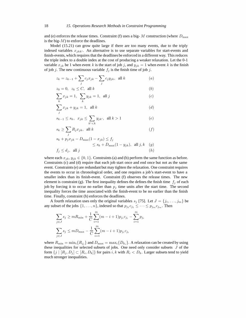
18 15. Operations Research Methods in Constraint Programming

and (e) enforces the release times. Constraint (f) uses a big-M construction (whereDmax

is the big-M ) to enforce the deadlines.Model (15.21) can grow quite large if there are too many events, due to the triply

indexed variablesxjkk′. An alternative is to use separate variables for start-events andfinish-events, which requires that the deadlines be enforced in a different way. This reducesthe triple index to a double index at the cost of producing a weaker relaxation. Let the 0-1variablexjk be 1 when eventk is the start of jobj, andyjk = 1 when eventk is the finishof job j. The new continuous variablefj is the finish time of jobj.

zk = zk−1 +∑

j

cjxjk −∑

j

cjyjk, all k (a)

z0 = 0, zk ≤ C, all k (b)∑

k

xjk = 1,∑

k

yjk = 1, all j (c)

∑

j

xjk + yjk = 1, all k (d)

sk−1 ≤ sk, xjk ≤∑

k′<k

yjk′ , all k > 1 (e)

sk ≥∑

j

Rjxjk, all k (f)

sk + pjxjk − Dmax(1 − xjk) ≤ fj

≤ sk + Dmax(1 − yjk), all j, k (g)fj ≤ dj , all j (h)

where eachxjk, yjk ∈ {0, 1}. Constraints (a) and (b) perform the same function as before.Constraints (c) and (d) require that each job start once and end once but not as the sameevent. Constraints (e) are redundant but may tighten the relaxation. One constraint requiresthe events to occur in chronological order, and one requires a job’s start-event to have asmaller index than its finish-event. Constraint (f) observes the release times. The newelement is constraint (g). The first inequality defines the defines the finish timefj of eachjob by forcing it to occur no earlier thanpj time units after the start time. The secondinequality forces the time associated with the finish-event to be no earlier than the finishtime. Finally, constraint (h) enforces the deadlines.

A fourth relaxation uses only the original variablessj [75]. Let J = {j1, . . . , jm} beany subset of the jobs{1, . . . , n}, indexed so thatpj1cj1 ≤ · · · ≤ pjmcjm . Then

∑

j∈J

sj ≥ mRmin +1C

m∑

i=1

(m − i + 1)pjicji −m∑

i=1

pji

∑

j∈J

sj ≤ mDmax − 1C

m∑

i=1

(m − i + 1)pjicji

whereRmin = mini{Rji} andDmax = maxi{Dki}. A relaxation can be created by usingthese inequalities for selected subsets of jobs. One need only consider subsetsJ of theform {j | [Rj, Dj ] ⊂ [Ri, Dk]} for pairsi, k with Ri < Dk. Larger subsets tend to yieldmuch stronger inequalities.

J. N. Hooker 19

15.7 Relaxation of Piecewise Linear and Disjunctive Constraints

Specialized relaxations can be devised for a number of additional constraints that com-monly occur in modeling. Two such constraints are bounds on piecewise linear, semicon-tinuous cost functions, and disjunctions of nonlinear inequality systems. There are alsoconvex hull relaxations (not discussed here) for various logical constraints [70], such ascardinality rules requiring that if at leastk of a given set of propositions are true, then atleast` of another set are true ([132], generalized in [10]).

15.7.1 Semicontinuous Piecewise Linear Functions

Piecewise linear functions are often useful in modeling, partly because they can approxi-mate nonlinear functions. A semicontinuous piecewise linear functionf(x) can be written

f(x) =Uk − x

Uk − Lkck +

x − Lk

Uk − Lkdk for x ∈ [Lk, Uk], k = 1, . . . , m

and is illustrated in Fig. 15.3.The functionf(x) can be given an MILP model by replacing all occurrences off(x)

with a new continuous variablev and writing

v =∑

k

λkak + µkbk, x =∑

k

λkLk + µkUk,∑

k

λk + µk = 1,∑

k

yk = 1

0 ≤ λk ≤ yk, 0 ≤ µk ≤ yk, all k

where eachyk ∈ {0, 1}. An LP relaxation is obtained by replacingyj ∈ {0, 1} by0 ≤ yj ≤ 1. The MILP model for continuous piecewise linear functions is slightly sim-pler; see [127]. An MILP model is used with a probe backtrack algorithm in [2].

Computational studies [101, 102, 105] suggest that it is often more efficient to writea convex hull relaxation directly in the original variables and dispense with the auxiliaryvariablesλk, µk, yk. One simply writes an inequality inv, x to represent each edge of theconvex hull, illustrated in Fig. 15.3.

15.7.2 Disjunctions of Nonlinear Systems

Methods for relaxing disjunctions of linear systems were presented in Section 15.4.3. Theyhave proved useful for relaxing problems that combine discrete and continuous linearelements. Many applications, however, mix discrete and continuousnonlinearelements.Fortunately, the convex hull relaxation for the linear case can be generalized to the convexnonlinear case. It has been used to solve several chemical process engineering problems[89, 90, 104, 112, 125]

The task is to relax∨

k∈K

gk(x) ≤ 0 (15.22)

wheregk(x) is a vector of convex functions andx ∈ <n. It is assumed thatx and eachgk(x) are bounded, and in particular thatL ≤ x ≤ U . A convex hull relaxation for (15.22)

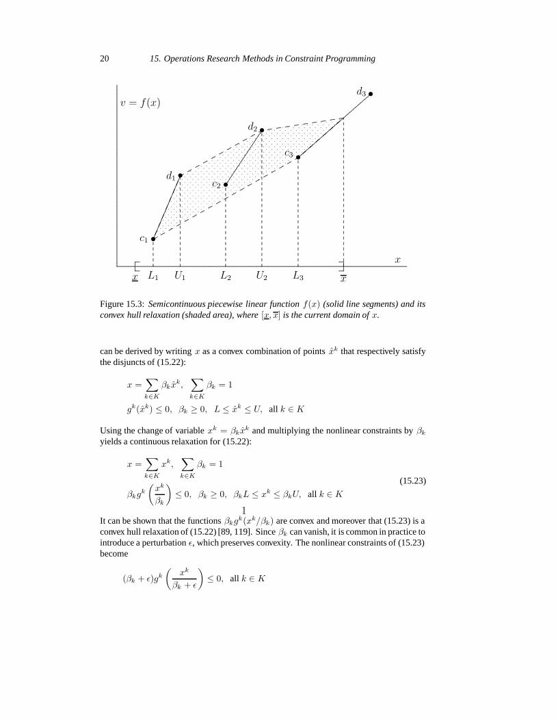
20 15. Operations Research Methods in Constraint Programming

......................................................................................................................................................................................................................................................................................................................................................................................................................................................................................................................................................................................................................................................................................................................................................................................................................................................................................................................................................................................................................................................................................................................................................................................................................................................................................................................................................x

v = f(x)

x xL1 U1 L2 U2 L3

c1

d1c2

d2

c3

d3

•

•

...............................................................................................................................................................................................

•

•

.....................................................................................................................................................................................

•

•

..........................................................................................................................................................................................................................................................................

....................................................

.................................................................................................................................................................................................................................................................................

........

........

........

........

........

........

........

........

........

........

........

........

........

........

........

........

........

........

........

........

........

........

........

........

........

........

........

........

........

........

........

........

........

........

........

........

........

........

........

........

........

........

........

........

........

........

........

........

........

........

........

........

........

........

........

........

........

........

........

........

........

........

........

........

........

........

........

........

........

........

........

........

........

........

........

........

........

........

........

........

........

........

..........................

..........................

..........................

..........................

..........................

..........................

..........................

..........................

..........................

...............................................................................................................................................................................................................................................................................................................................................................

..........................

..........................

..........................

.............. .

. ...

.

.

.

.

.

.

.

.

.

.

.

.

.

.

.

.

.

.

.

.

.

.

.

.

.

.

.

.

.

.

.

.

.

.

.

.

.

.

.

.

.

.

.

.

.

.

.

.

.

.

.

.

.

.

.

.

.

.

.

.

.

.

.

.

.

.

.

.

.

.

.

.

.

.

.

.

.

.

.

.

.

.

.

.

.

.

.

.

.

.

.

.

.

.

.

.

.

.

.

.

.

.

.

.

.

.

.

.

.

.

.

.

.

.

.

.

.

.

.

.

.

.

.

.

.

.

.

.

.

.

.

.

.

.

.

.

.

.

.

.

.

.

.

.

.

.

.

.

.

.

.

.

.

.

.

.

.

.

.

.

.

.

.

.

.

.

.

.

.

.

.

.

.

.

.

.

.

.

.

.

.

.

.

.

.

.

.

.

.

.

.

.

.

.

.

.

.

.

.

.

.

.

.

.

.

.

.

.

.

.

.

.

.

.

.

.

.

.

.

.

.

.

.

.

.

.

.

.

.

.

.

.

.

.

.

.

.

.

.

.

.

.

.

.

.

.

.

.

.

.

.

.

.

.

.

.

.

.

.

.

.

.

.

.

.

.

.

.

.

.

.

.

.

.

.

.

.

.

.

.

.

.

.

.

.

.

.

.

.

.

.

.

.

.

.

.

.

.

.

.

.

.

.

.

.

.

.

.

.

.

.

.

.

.

.

.

.

.

.

.

.

.

.

.

.

.

.

.

.

.

.

.

.

.

.

.

.

.

.

.

.

.

.

.

.

.

.

.

.

.

.

.

.

.

.

.

.

.

.

.

.

.

.

.

.

.

.

.

.

.

.

.

.

.

.

.

.

.

.

.

.

.

.

.

.

.

.

.

.

.

.

.

.

.

.

.

.

.

.

.

.

.

.

.

.

.

.

.

.

.

.

.

.

.

.

.

.

.

.

.

.

.

.

.

.

.

.

.

.

.

.

.

.

.

.

.

.

.

.

. ..

.

. .... . .

1

Figure 15.3:Semicontinuous piecewise linear functionf(x) (solid line segments) and itsconvex hull relaxation (shaded area), where[x, x] is the current domain ofx.

can be derived by writingx as a convex combination of pointsxk that respectively satisfythe disjuncts of (15.22):

x =∑

k∈K

βkxk,∑

k∈K

βk = 1

gk(xk) ≤ 0, βk ≥ 0, L ≤ xk ≤ U, all k ∈ K

Using the change of variablexk = βkxk and multiplying the nonlinear constraints byβk

yields a continuous relaxation for (15.22):

x =∑

k∈K

xk,∑

k∈K

βk = 1

βkgk

(xk

βk

)≤ 0, βk ≥ 0, βkL ≤ xk ≤ βkU, all k ∈ K

(15.23)

It can be shown that the functionsβkgk(xk/βk) are convex and moreover that (15.23) is aconvex hull relaxation of (15.22) [89, 119]. Sinceβk can vanish, it is common in practice tointroduce a perturbationε, which preserves convexity. The nonlinear constraints of (15.23)become

(βk + ε)gk

(xk

βk + ε

)≤ 0, all k ∈ K

J. N. Hooker 21

One can also relax (15.22) with a big-M relaxation similar to the LP relaxation of(15.11):

gk(x) ≤ Mk(1 − βk), βk ≥ 0, all k ∈ K∑

k∈K

βk = 1

where each component ofMk is an upper bound on the corresponding function ingk(x).

15.8 Lagrangean Relaxation

Many relaxations are formed simply by removing constraints.Lagrangean relaxationrefines this process by imposing a penalty for violation of the deleted constraints, providedthey have inequality form. This tends to make the minimum value of the relaxed prob-lem larger and may therefore provide a tighter bound on the optimal value of the originalproblem.

A Lagrangean relaxation is actually a family of relaxations, since one can choose thepenalty (i.e., the Lagrange multiplier) for each constraint violation. The problem of select-ing the multipliers that result in the tightest bound is theLagrangean dual.

Since solution of the Lagrangean dual tends to be time consuming, the general prac-tice in CP applications is to solve it only at the root node and use the resulting Lagrangemultipliers at all subsequent nodes. These multipliers not only define a relaxation that canbe quickly solved or propagated, but they allow domain filtering in the same fashion as thedual multipliers of an LP relaxation. In fact, dual multipliers are a special case of Lagrangemultipliers.

Lagrangean relaxation is particularly useful in CP when a full linear relaxation is in-compatible with the very rapid processing of search tree nodes that often characterizesCP methods. In such cases one may be able to solve a Lagrangean dual of the LP at theroot node, which is itself an LP problem, to obtain a weaker but specially-structured LPrelaxation that can be solved quickly at the remaining nodes.

CP-based Lagrangean methods have been applied to network design [36], automaticdigital recording [113], traveling tournament problems [17], the resource-constrainedshort-est path problem [54], and the general problem of filtering domains [85].

15.8.1 The Lagrangean Dual

Lagrangean relaxation is applied to problems of the form

min f(x)gi(x) ≤ 0, i = 1, . . . , m

x ∈ S, x ∈ <n

(15.24)

wherex ∈ S represents an arbitrary constraint set but in practice is carefully chosen to havespecial structure. Lagrangean relaxationdualizesthe constraintsgi(x) ≤ 0 by penalizingtheir violation in the objective function:

min θ(x, λ) = f(x) +m∑

i−1

λigi(x)

x ∈ S, x ∈ <n

(15.25)

22 15. Operations Research Methods in Constraint Programming

where eachλi ≥ 0 is aLagrange multiplier. The motivation for using the relaxation is thatthe special structure of the constraintsx ∈ S makes it easy to solve. The term “penalty”is not quite right for the expressionλigi(x), however, since a penalty should vanish whenthe solution is feasible;λigi(x) can go negative whenx is feasible, resulting in a “saddle”function.

Clearlyθ(x, λ) ≤ f(x) for anyx that is feasible in the relaxation (15.25), sinceλ ≥ 0and eachgi(x) ≤ 0. Thus for anyλ ≥ 0, the optimal valueθ(λ) of the Lagrangeanrelaxation (15.25) is a lower bound on the optimal valuev∗ of the original problem (15.24)(weak duality). The tightest lower bound onv∗ is obtained by solving theLagrangean dualproblem: maximizeθ(λ) subject toλ ≥ 0. The amount by which this bound falls short ofv∗ is theduality gap.

15.8.2 Solving the Dual

Since the Lagrangean functionθ(λ) is concave, it can be maximized by finding a localmaximum. A popular approach issubgradient optimization, which begins with a startingvalueλ0 ≥ 0 and sets eachλk+1 = λk + αkσk, whereσk is a subgradient ofθ(λ) atλ = λk. Conveniently, ifθ(λk) = f(xk, λ), then(g1(xk), . . . , gm(xk)) is a subgradient.The stepsizeαk should decrease ask increases, but not so quickly as to cause prematureconvergence. A simple option is to setαk = α0/k, or perhapsαk = α0(θ−θ(λk))/||σk||,whereθ is a dynamically adjusted upper bound on the maximum value ofθ(λ). The step-size is highly problem-dependent and must be tuned for every problem class. Solutionmethods are further discussed in [11, 98].

Typically the Lagrangean dual is solved only at the root node. As one descends intothe search tree, branching adds constraints to the problem, and the dual solutionλ∗ ceasesto be optimal. Nonetheless the optimal value of the Lagrangean relaxation, withλ set toλ∗ and branching constraints added, continues to be a valid lower bound of the optimalsolution. In fact there is no need to obtain optimalλis even at the root node, and frequentlythe subgradient algorithm is terminated early.

One must take care that branching constraints do not destroy the special structure ofthe Lagrangean relaxation. For instance, one may wish to branch by fixing one or variablesrather than adding inequality constraints.

15.8.3 Special Case: Linear Programming

The Lagrangean dual of an LP problem is easy to solve, since it is equivalent to the LPdual. Suppose the original problem (15.24) is an LP problem

min cx

Ax ≥ b, Dx ≥ d, x ≥ 0(15.26)

in which the linear systemDx ≥ d has some kind of special structure. IfAx ≥ b isdualized, thenθ(λ) is the optimal value of

min θ(x, λ) = cx + λ(b − Ax) = (c − λA)x + λb

Dx ≥ d, x ≥ 0(15.27)

J. N. Hooker 23

Supposex∗ is an optimal solution of the original LP problem (15.26), and(λ∗, µ∗) is anoptimal dual solution in whichλ∗ corresponds toAx ≥ b andµ∗ to Dx ≥ d. Thus

cx∗ = λ∗b + µ∗d (15.28)

by strong duality. It will be shown below thatθ(λ∗) = cx∗. This implies thatλ∗ is anoptimal dual solution of the Lagrangean dual problem, sinceθ(λ) is a lower bound oncx∗

for anyλ ≥ 0.One can therefore solve the Lagrangean dual of (15.26) at the root node by solving

its LP dual. If(λ∗, µ∗) solves the LP dual, thenλ∗ solves the Lagrangean dual in whichAx ≥ b is dualized. At subsequent nodes one solves the specially structured LP problem(15.27), withλ set to the valueλ∗ obtained at the root node, to obtain a valid lower boundon the value of the LP relaxation at that node.

To see thatθ(λ∗) = cx∗, note first thatx∗ is feasible in

minx≥0

{(c − λ∗A)x | Dx ≥ d} (15.29)

andµ∗ is feasible in its LP dual

maxµ≥0

{ud | µD ≤ c − λ∗A} (15.30)

where the latter is true because(λ∗, µ∗) is dual feasible for (15.26). But the correspondingobjective function value of (15.29) is

(c − λ∗)x∗ = cx∗ + λ∗(b − Ax∗) − λ∗b = cx∗ − λ∗b

where the second equation is due to complementary slackness. This is equal to the valueµ∗d of (15.30), due to (15.28). Socx∗ − λ∗b is the optimal value of (15.29), which meansthatcx∗ is the optimal valueθ(λ∗) of (15.27) whenλ = λ∗.

15.8.4 Domain Filtering

Lagrangean duality provides a generalization of the filtering mechanism based on LP dual-ity. Suppose that there is an upper boundU on the costf(x) in (15.24), and letv∗ = θ(λ∗)be the optimal value of the Lagrangean dual. Letx∗ solve (15.25) whenλ = λ∗, sothat θ(λ∗) = θ(λ∗, x∗), and suppose further thatgi(x∗) = 0. If the solution of (15.24)were to change, functiongi(x) could decrease, say by an amount∆i. This would in-crease the optimal value of (15.24) as much as changing the the constraintgi(x) ≤ 0 togi(x) + ∆i ≤ 0. The functionθ(λ) for the altered problem isθ′(λ) = minx∈S{θ′(λ, x)},whereθ′(λ, x) = f(x) +

∑j λjgj(x) + λi∆i. Sinceθ′(λ∗, x) differs fromθ(λ∗, x) only

by a constant, anyx that minimizesθ(λ∗, x) also minimizesθ′(λ∗, x). So

θ′(λ∗) = θ′(λ∗, x∗) + λ∗i ∆i = v∗ + λ∗

i ∆i

is a lower bound on the optimal value of the altered problem, by weak duality. Thus onemust havev∗ + λ∗∆i ≤ U , or∆i ≤ (U − v∗)/λ∗

i . Since∆i = gi(x∗)− gi(x) = −gi(x),this yields a valid inequality parallel to (15.6) that can be propagated:

gi(x) ≥ −U − v∗

λ∗i

(15.31)

If constrainti imposes a lower boundL on a variablexj (i.e., −xj + L ≤ 0), then(15.31) becomesxj ≤ L + (U − v∗)/λ∗

i . This can be used to reduce the domain ofxj ifλ∗

i > 0, and similarly if there is an upper bound onxj.

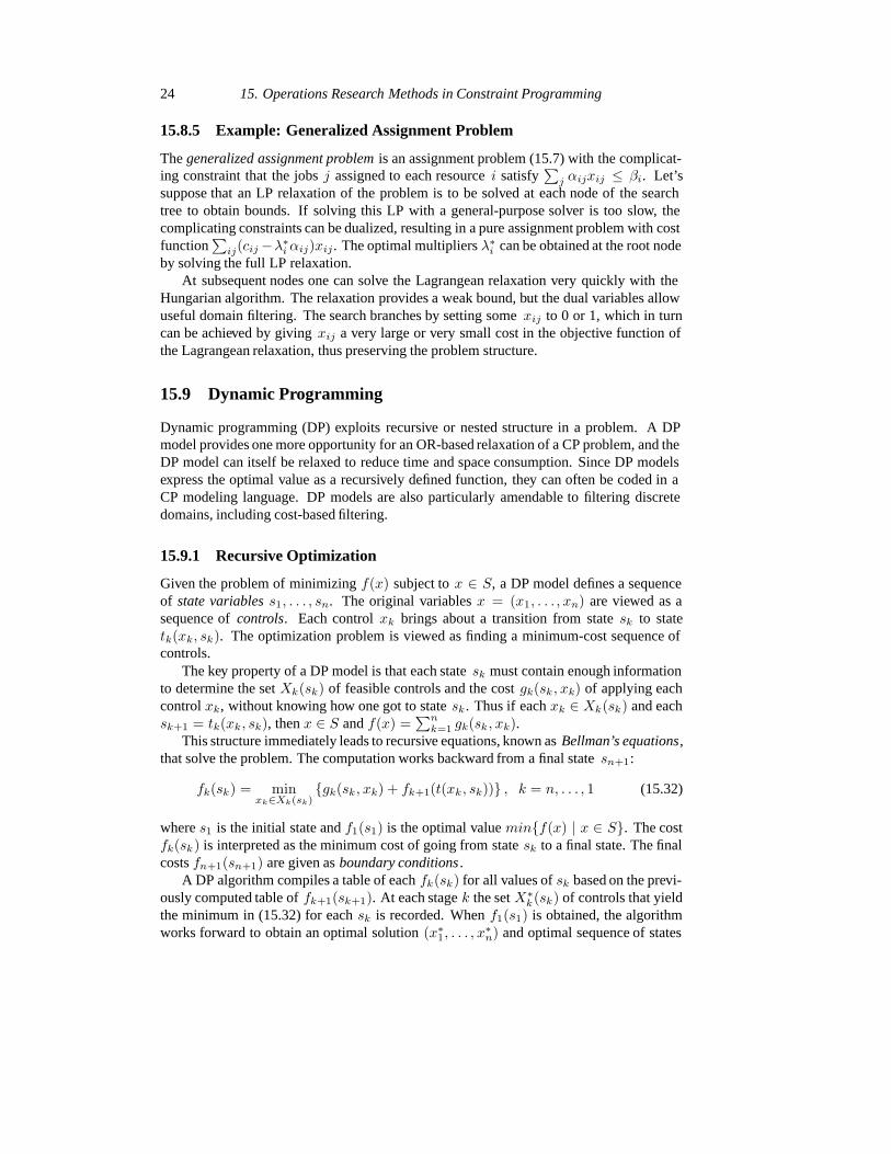
24 15. Operations Research Methods in Constraint Programming

15.8.5 Example: Generalized Assignment Problem

Thegeneralized assignment problemis an assignment problem (15.7) with the complicat-ing constraint that the jobsj assigned to each resourcei satisfy

∑j αijxij ≤ βi. Let’s

suppose that an LP relaxation of the problem is to be solved at each node of the searchtree to obtain bounds. If solving this LP with a general-purpose solver is too slow, thecomplicating constraints can be dualized, resulting in a pure assignment problem with costfunction

∑ij(cij −λ∗

i αij)xij. The optimal multipliersλ∗i can be obtained at the root node

by solving the full LP relaxation.At subsequent nodes one can solve the Lagrangean relaxation very quickly with the

Hungarian algorithm. The relaxation provides a weak bound, but the dual variables allowuseful domain filtering. The search branches by setting somexij to 0 or 1, which in turncan be achieved by givingxij a very large or very small cost in the objective function ofthe Lagrangean relaxation, thus preserving the problem structure.

15.9 Dynamic Programming

Dynamic programming (DP) exploits recursive or nested structure in a problem. A DPmodel provides one more opportunity for an OR-based relaxation of a CP problem, and theDP model can itself be relaxed to reduce time and space consumption. Since DP modelsexpress the optimal value as a recursively defined function, they can often be coded in aCP modeling language. DP models are also particularly amendable to filtering discretedomains, including cost-based filtering.

15.9.1 Recursive Optimization

Given the problem of minimizingf(x) subject tox ∈ S, a DP model defines a sequenceof state variabless1, . . . , sn. The original variablesx = (x1, . . . , xn) are viewed as asequence ofcontrols. Each controlxk brings about a transition from statesk to statetk(xk, sk). The optimization problem is viewed as finding a minimum-cost sequence ofcontrols.

The key property of a DP model is that each statesk must contain enough informationto determine the setXk(sk) of feasible controls and the costgk(sk, xk) of applying eachcontrolxk, without knowing how one got to statesk. Thus if eachxk ∈ Xk(sk) and eachsk+1 = tk(xk, sk), thenx ∈ S andf(x) =

∑nk=1 gk(sk, xk).

This structure immediately leads to recursive equations, known asBellman’s equations,that solve the problem. The computation works backward from a final statesn+1:

fk(sk) = minxk∈Xk(sk)

{gk(sk, xk) + fk+1(t(xk, sk))} , k = n, . . . , 1 (15.32)

wheres1 is the initial state andf1(s1) is the optimal valuemin{f(x) | x ∈ S}. The costfk(sk) is interpreted as the minimum cost of going from statesk to a final state. The finalcostsfn+1(sn+1) are given asboundary conditions.

A DP algorithm compiles a table of eachfk(sk) for all values ofsk based on the previ-ously computed table offk+1(sk+1). At each stagek the setX∗

k(sk) of controls that yieldthe minimum in (15.32) for eachsk is recorded. Whenf1(s1) is obtained, the algorithmworks forward to obtain an optimal solution(x∗

1, . . . , x∗n) and optimal sequence of states

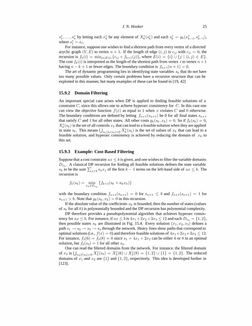
J. N. Hooker 25

s∗1, . . . , s∗n by letting eachx∗

k be any element ofX∗k (s∗k) and eachs∗k = gk(x∗

k−1, s∗k−1),

wheres∗1 = s1.For instance, suppose one wishes to find a shortest path from every vertex of a directed

acyclic graph(V, E) to vertexn + 1. If the length of edge(i, j) is cij with cii = 0, therecursion isfk(i) = minj∈E(i) {cij + fk+1(j)}, whereE(i) = {i} ∪ {j | (i, j) ∈ E}.The costfk(i) is interpreted as the length of the shortest path from vertexi to vertexn + 1havingn − k + 1 or fewer edges. The boundary condition isfn+1(n + 1) = 0.

The art of dynamic programming lies in identifying state variablessk that do not havetoo many possible values. Only certain problems have a recursive structure that can beexploited in this manner, but many examples of these can be found in [19, 42]

15.9.2 Domain Filtering

An important special case arises when DP is applied to finding feasible solutions of aconstraintC, since this allows one to achieve hyperarc consistency forC. In this case onecan view the objective functionf(x) as equal to 1 whenx violatesC and0 otherwise.The boundary conditions are defined by lettingfn+1(sn+1) be 0 for all final statessn+1

that satisfyC and1 for all other states. All other costsgk(sk, xk) = 0. So if fk(sk) = 0,X∗

k(sk) is the set of all controlsxk that can lead to a feasible solution when they are appliedin statesk. This means

⋃sk|fk(sk)=0 X∗

k (sk) is the set of values ofxk that can lead to afeasible solution, and hyperarc consistency is achieved by reducing the domain ofxk tothis set.

15.9.3 Example: Cost-Based Filtering

Suppose that a cost constraintax ≤ b is given, and one wishes to filter the variable domainsDxk . A classical DP recursion for finding all feasible solutions defines the state variablesk to be the sum

∑j<k ajxj of the firstk − 1 terms on the left-hand side ofax ≤ b. The

recursion is

fk(sk) = minxk∈Dxk

{fk+1(sk + akxk)}

with the boundary conditionfn+1(sn+1) = 0 for sn+1 ≤ b andfn+1(sn+1) = 1 forsn+1 > b. Note thatgk(sk, xk) = 0 in this recursion.

If the absolute value of the coefficientsak is bounded, then the number of states (valuesof sk for all k) is polynomially bounded and the DP recursion has polynomial complexity.

DP therefore provides a pseudopolynomial algorithm that achieves hyperarc consis-tency forax ≤ b. For instance, ifax ≤ b is 4x1+2x2 +3x3 ≤ 12 and eachDxk = {1, 2},then possible statessk are illustrated in Fig. 15.4. Every solution(x1, x2, x3) defines apaths1 → s2 → s3 → s4 through the network. Heavy lines show paths that correspond tooptimal solutions (i.e.,f(x) = 0) and therefore feasible solutions of4x1+2x2+3x3 ≤ 12.For instance,f3(6) = f3(8) = 0 sinces3 = 4x1 + 2x2 can be either6 or 8 in an optimalsolution, butf3(s3) = 1 for all others3.

One can read the filtered domains from the network. For instance, the filtered domainof x3 is

⋃s3|f(s3)=0 X∗

3 (s3) = X∗3 (6) ∪ X∗

3 (8) = {1, 2} ∪ {1} = {1, 2}. The reduceddomains ofx1 andx2 are{1} and{1, 2}, respectively. This idea is developed further in[123].

26 15. Operations Research Methods in Constraint Programming

0

8

4

12

10

8

6

18

16

15

14

13

12

11

9

.....................................................................................................................................................................................

.....................................................................................................................................................................................

.....................................................................................................................................................................................

.................................

.................................

.................................

.............................

.......................................................................................................................................

.......................................................................................................................................

................................................................................................................................

...................................

...................................

...................................

..............................

...................................

...................................

...................................

..............................

..................................................................

...........................................

...........................................................................................................................

...........................................................................................................................

..................................................................................................................................................

.......................................................................................................................................................

.......................................................................................................................................................

..................................................................................................................................................

.......................................................................................................................................................

.......................................................................................................................................................

..................................................................................................................................................

.......................................................................................................................................................

k = 1 2 3 4

1

Figure 15.4:Statessk for the constraint4x1 + 2x2 + 3x3 ≤ 12 with xj ∈ {1, 2}. Edgesleaving state 0 correspond tox1 = 1, 2, and similarly for other edges. Costs associ-ated with the terminal states (k = 4) are 0 for the boldface states and 1 for the others.Heavy lines correspond to paths that lead to optimal solutions (i.e. solutions feasible for4x1 + 2x2 + 3x3 ≤ 12).

15.9.4 State Space Relaxation

When the state variablessk have too many values,state space relaxationcan reduce thenumber of values and make the problem easier to solve. State space relaxation in ef-fect uses a hash code for the states; it defines a functionφ(sk) that maps many values ofsk to the same state. Every controlxk ∈ Xk(sk) is mapped to a control that takes thesystem fromφ(sk) to φ(gk(sk, xk)). The cost functiongk for the relaxation must satisfygk(φ(sk), φ(yk)) ≤ gk(sk, xk). The optimal value of the relaxed problem is a lower boundon the optimal value of the original recursion.

This can be illustrated by relaxing a DP formulation of the traveling salesman problemon a graph(V, E). The objective is to minimize

∑i cxixi+1 subject to alldiff(x1, . . . , xn)

and(xi, xi+1) ∈ E. Letx1 be the first customer visited after leaving home basei0, and fixthe last customer visitedxn to be home base. The classical DP formulation defines statevariablesk to be(i, Vk), whereVk is any set ofn − k + 1 vertices andi ∈ Vk. The costfk(i, Vk) is interpreted as the cost of the minimum-cost tour that starts ati and covers all

J. N. Hooker 27

the vertices inVk. If Ei = {j | (i, j) ∈ E}, the recursion is

fk(i, Vk) = minxk∈(Vk∩Ei)\{i}

{cixk + fk+1(xk, Vk \ {i})} (15.33)

with boundary conditionfn(i, {i}) = cii0 for all verticesi with i0 ∈ Ei andfn(i, {i}) =∞ for all otheri.

The recursion (15.33) is not computationally useful because there are exponentiallymany states(i, Vk). However, this DP model can be relaxed, for example by mapping allstates(i, Vk) for a givenk to φ(i, Vk) = (i, k). The cost of a transition from(i, k) to(j, k + 1) is the same as that from any(i, Vk) to any(j, Vk+1), namelycij. The recursion(15.33) becomes

fk(i) = minxk∈Ei

{cixk + fk+1(xk)

}(15.34)

with the same boundary condition as before. A CP solution of (15.34) and other issues arediscussed in [53].

15.9.5 Nonserial Dynamic Programming

DP is based on the principle that each statesk depends only on the previous statesk−1 andcontrolxk−1. In nonserial dynamic programming(NSDP), a state may depend on severalprevious states.

NSDP has been known in OR for more than 30 years [18]. Essentially the same ideahas surfaced in a number of contexts, including Bayesian networks [88], belief logics [115,117], pseudoboolean optimization [35], location theory [28],k-trees [7, 8], and bucketelimination [39].

In the simplest form of NSDP, the state variablessk are the original variablesxk. Thisis the form most relevant to CP, since it permits solution of a constraint setC in time thatis directly related to the width of the dependency graphG of C.

The width of a directed graphG is the maximum in-degree of vertices ofG. Theinduced widthof G with respect to an ordering of vertices1, . . . , n is the width ofG′ withrespect to this ordering, whereG′ is constructedas follows. Remove verticesn, n−1, . . . , 1from G one a time, and when each vertexi is removed, add edges as necessary so that thevertices adjacent toi at the time of its removal form a clique. ThenG′ consists ofG plusall edges added in this process.

The dependency graphG for constraint setC contains a vertex for each variablexj ofC and an edge(xi, xj) whenxi andxj occur in a common constraint. LetSk be the set ofvertices in{1, . . . , k − 1} that are adjacent tok in G′, and letxi be the set of variables inconstraintCi ∈ C. Define the cost functionci(xi) to be 1 ifxi violatesCi and 0 otherwise.Then the NSDP recursion again works backward:

fk(Sk) = minxk∈Dxk

∑

i∈Ik

ci(xi) +∑

j∈Jk

fj(Sj)

, k = 1, . . . , n (15.35)

whereIk is the set of indicesi for whichxi containsxk but none ofxk+1, . . . , xn. Jk is theset of indicesj ∈ {k + 1, . . . , . . . , n} for whichSj containsxk but none ofxk+1, . . . , xn.Note that the computation offk(Sk) may use previously computed costsfi(Si) for several

28 15. Operations Research Methods in Constraint Programming

i ∈ {k + 1, . . . , n}. The process gets started by computingfn(Sn), which requires noprevious results. The optimal value

∑k|Sk=∅ fk(∅) is 0 if and only if C has a feasible

solution. A feasible solution is recovered by recording for eachk the setX∗k (Sk) of values

of xk that achieve the minimum value of zero in (15.35). The fork = 1, . . .n one canselect anyx∗

k ∈ X∗k (S∗

k), whereS∗k contains the previously selected values forxj ∈ Sk.

The complexity of the recursion (15.35) is at worst proportional tonDw+1, whereD isthe size of the largest variable domain, andw is the size of the largest setSk. But w is thewidth of G′ and therefore the induced with ofG with respect to the orderingx1, . . . , xn.So the complexity of solving a constraint setC by NSDP is at worst exponential in theinduced width ofC ’s dependency graph with respect to the reverse order of recursion.These ideas are further discussed in [70].

15.10 Branch-and-Price Methods

Branch and priceis a well-known OR technique that is applied to MILP problems witha very large number of variables. In fact, the MILP model is sometimes reformulatedso as to have exponentially many variables, since this may simplify the model while yetallowing solution by branch and price.

The basic idea is to solve the MILP initially with only a few variables, and add variablesto the problem as they are needed to improve on the current solution. A subproblem issolved to identify promising variables. Since a variable is added to the problem by adding acolumn to the MILP constraint matrix, this approach is often known ascolumn generation.Complicating constraints can be dealt with implicitly by restricting what sort of columnscan be generated by the subproblem.

It is in the column generation phase that CP can be useful, since the subproblem mayhave complicated constraints that make it more amenable to solution by CP rather thanOR methods. CP-based branch and price has proved successful in several applications thatinvolve assignment of resources under complex constraints.

15.10.1 The Algorithm

Branch and price is applied to an MILP problem

min cy

Ay = b, y ≥ 0, y` integer for` ∈ I(15.36)

whereI ⊂ {1, . . . , n}. The algorithm is a branch-and-bound search that solves the LPrelaxation at each node of the search tree by column generation.

The column generation procedure begins with an LP relaxation that contains a subsetof the variables:

min∑

`∈L

c`y`

∑

`∈L

A`y` = b; y` ≥ 0, ` ∈ L(15.37)

whereA` is column` of A andL ⊂ {1, . . . , n}. If λ∗ = (λ∗1, . . . , λ

∗m) is the optimal

dual solution of (15.37), then any nonbasic variabley` has reduced costc` − λ∗A` (see

J. N. Hooker 29

Section 15.3). A subproblem is solved to find a column(c`, A`) with the smallest reducedcost. Thus the subproblem minimizesz0 −

∑mi=1 λ∗

i zi subject to(z0, z1, . . . , zm) ∈ Z,whereZ is the set of all columns(c`, A`). If a column with negative reduced cost is found,it is added to (15.37). The process is repeated until no column with negative reduce costis found in the subproblem, whereupon (15.37) is solved. If all goes well, only a smallfraction of the columns ofA will have been generated.

15.10.2 Example: Generalized Assignment Problem

Most applications of branch and price involve an assignment problem with complicatingconstraints. One example is the generalized assignment problem, which again is an as-signment problem (15.7) with the complicating constraint that the jobsj assigned to eachresourcei satisfy

∑j αijxij ≤ βi.

The problem is reformulated for branch and price by lettingk index all possible assign-ments of jobs to a given resourcei that satisfy

∑j αijxij ≤ βi. The 0-1 variableyik = 1

if the kth assignment to resourcei is selected. So ifδijk = 1 when jobj is assigned toresourcei in assignmentk, an LP relaxation of the problem has the form (15.36) with` = (i, k):

min∑

ik

∑

j

cijδijk

yik

∑

ik

δijkyik = 1, all j (a)

∑

k

yik = 1, all i (b)

yik ≥ 0, all i, k

(15.38)

If dual variablesλj are associated with constraints (a) andµi with constraints (b), thereduced cost of a variableyik in (15.38) is

∑

j

cijδijk −∑

j

λjδijk − µi =∑

j

(cij − λj)δijk − µi

The subproblem of finding a variableyik with negative reduced cost can be solved byexamining each resourcei separately and solving the 0-1 knapsack problem

min∑

j

(cij − λj)zj − µi

∑

j

αijzj ≤ βi; zj ∈ {0, 1}, all j

0-1 knapsack problems can be solved by a number of methods [95], including CP [48].

15.10.3 Other Applications

One of the most successful applications of CP-based branch and price is to airline crewassignment and crew rostering [26, 47, 82, 87, 114]. In [47], for example, a path constraint

30 15. Operations Research Methods in Constraint Programming

is used to obtain a permissible roster with a negative reduced cost. The search tree ispruned by solving a relaxation of the problem (a single-source shortest path problem) soas to obtain a lower bound on the reduced cost.

CP-based branch and price has also been applied to transit bus crew scheduling [133],aircraft scheduling [59], vehicle routing [109], network design [27], employee timetabling[41], physician scheduling [55], and the traveling tournament problem [43, 44]. Severalimplementation issues are discussed in [45, 108].

15.11 Benders Decomposition

Benders decomposition was developed in the context of mathematical programming, butthe root idea has much wider application. It solves a problem by enumerating, in amasterproblem, possible values of a pre-selected subset of variables. Each set of values that mightbe assigned to these variables defines thesubproblemof finding the best values for theremaining variables. Solution of the subproblem generates a nogood, known as aBenderscut, that excludes that particular assignment to the master problem variables, and perhapsother assignments that can be no better. The master problem is re-solved with the newBenders cut in order to find a better solution, and the process continues until no furtherimprovement is possible.

Benders decomposition can profitably combine OR and CP, since one approach canbe applied to the master problem and one to the subproblem, depending on which bestsuits the problem structure. This sort of combination has yielded substantial speedups incomputation.

15.11.1 Benders Decomposition in the Abstract

In classical Benders decomposition, the subproblem is a linear or nonlinear programmingproblem [15, 56], and the Benders cuts are generated using dual or Lagrange multipliers.However, if one recognizes that LP duality is a special case of a more generalinferenceduality, the concept of a Benders cut can be generalized [70, 80]. In fact the basic idea ofBenders decomposition is best seen in this more general setting and then specialized to theclassical case.

Benders decomposition applies to problems of the form

min f(x, y)(x, y) ∈ S, x ∈ Dx, y ∈ Dy

(15.39)

Each iterationk of the Benders algorithm begins with a fixed valuexk for x and solves asubproblem for the besty:

min f(xk, y)(xk, y) ∈ S, y ∈ Dy

(15.40)

Solution of the subproblem yields an optimal solutionyk and an optimal valuevk =f(xk, yk). The solution process is analyzed to identify a proof thatf(xk, y) ≥ vk; such aproof can be regarded as solving the inference dual of (15.40). (The inference dual of anLP problem is the classical LP dual.) Ifxk is changed to some other valuex, this sameproof may still show thatf(x, y) is bounded below by some functionBk(x). This yields

J. N. Hooker 31

the Benders cutz ≥ Bk(x), whereBk(xk) = vk andz is a variable indicating the optimalvalue of the original problem (15.39).

At this point one solves the master problem, which contains the Benders cuts so fargenerated.

min z

z ≥ Bi(x), i = 1, . . .k, x ∈ Dx(15.41)

The solutionxk+1 of (15.41) begins the next iteration. Since the master problem (15.41) isa relaxation of the original problem and the subproblem (15.40) a restriction if it, the opti-mal valuezk+1 of the master problem is a lower bound on the optimal value of (15.39), andthe optimal value of any subproblem is an upper bound. The algorithm terminates with anoptimal solution when the two bounds converge; that is, whenzk+1 = mini∈{1,...,k}{vi}.They converge finitely under fairly weak conditions, for instance if the domainDx is finite,as it is in examples considered here.

15.11.2 Classical Benders Decomposition

The historical Benders decomposition applies to problems of the form

min f(x) + cy

g(x) + Ay ≥ b, x ∈ S, y ≥ 0, x ∈ Dx, y ∈ <n

The subproblem (15.40) is the LP problem

min f(xk) + cy

Ay ≥ b − g(xk), y ≥ 0, y ∈ <n (15.42)

Suppose first that (15.42) has optimal valuevk and an optimal dual solutionλk. By strongdualityvk − f(xk) = λk(b − g(xk)), which means

Bk(x) = f(x) + λk(b − g(x)) (15.43)

is the tightest lower bound on cost whenx = xk. That is,λk specifies a proof of thelower boundvk by defining a linear combinationλkAy ≥ λk(b − g(xk)) that dominatescy ≥ vk − f(xk). But sinceλk remains dual feasible whenxk in (15.42) is replaced byanyx, (15.43) remains a lower bound on cost for anyx; that is,λk specifies a proof of thelower boundBk(x). This yields the Benders cut

z ≥ f(x) + λk(b − g(x)) (15.44)

If the dual of (15.42) is unbounded, there is a direction or rayλk along which its solutionvalue can increase indefinitely. In this case the Benders cut isλk(b − g(x)) ≤ 0 rather than(15.44). The Benders cutsz ≥ Bk(x) in the master problem (15.41) therefore take the form(15.44) when the subproblem dual is bounded in iterationk, and the formλk(b−g(x)) ≤ 0when the subproblem dual is unbounded. The master problem can be solved by any desiredmethod, such as branch and bound if it is an MILP problem.

32 15. Operations Research Methods in Constraint Programming

15.11.3 Example: Planning and Scheduling

A basic planning and scheduling problem illustrates the use of nonclassical Benders tocombine MILP and CP [71]. Eachn jobs must be assigned to one ofm facilities forprocessing. Each jobj has processing timepij and usescij units of resource on facilityi. Every job has release time 0 and deadlined. Jobs scheduled on any facilityi may runsimultaneously so long as the total resource consumption at any one time is no greater thanCi (cumulative scheduling). The objective is to minimize makespan (i.e., finish the last jobas soon as possible).

If job j has start timesj on machineyj , the problem can be written

min z

z ≥ sj + pyjj, 0 ≤ sj ≤ d − pyjj, all j

cumulative(si(y), pi(y), ci(y), Ci

), all i

wheresi(y) = (sj | yj = i) and similarly forpi(y), ci(y).The master problem assigns jobs to facilities and is well suited for MILP solution. The

subproblem schedules jobs assigned to each facility and is suitable for a CP approach.Given an assignmentyk obtained by solving the master problem, the subproblem sep-

arates into an independent scheduling problem for each facilityi:

min zi

zi ≥ si + pij, 0 ≤ sj ≤ d − pij, all j ∈ Jki

cumulative(si(yk), pi(yk), ci(yk), Ci)

whereJki = {j | ykj = i} is the set of jobs assigned to facilityi. Let zik be the optimal

makespan obtained in the subproblemPi for facility i. A Benders cut can be constructedby reasoning as follows.

First let Pi be the problem that results when jobs in setR are removed from problemPi, and letz be the optimal makespan forPi. Then

z ≥ zik − ∆ (15.45)

where∆ =∑

j∈R pij. To see this, construct a solutionS for Pi by scheduling the jobs in

R sequentially after the last job in the optimal solution ofPi. The resulting makespan isz + ∆. If z + ∆ ≤ d, thenS is feasible forPi, so thatzik ≤ z + ∆ and (15.45) follows.On the other hand, ifz + ∆ > d, then (15.45) follows becausezik ≤ d.

Since the master problem will be solved by MILP, it is convenient to write the Benderscuts in terms of 0-1 variablesxij, wherexij = 1 whenyj = i. In subsequent iterations ofthe Benders algorithm, the jobs inJki that are removed from facilityi are those for whichxij = 0. So (15.45) yields the following lower bound on the minimum makespanz forfacility i, which is also a lower bound on the minimum makespanz for the problem as awhole:

z ≥ zik −∑

j∈Jki

pij(1 − xij) (15.46)

J. N. Hooker 33

Each Benders cutz ≥ Bk(x) in the master problem is therefore actually a set of inequali-ties (15.46), one for each facilityi. The master problem becomes

min z∑

i

xij = 1, all j (a)

z ≥ zi` −∑

j∈Ji`

pij(1 − xij), all i, ` = 1, . . . , k (b)

z ≥1Ci

n∑

j=1

cijpijxij, all i (c)

(15.47)

The expression (c) is a simple relaxation of the subproblem, which can be important toobtain good computational performance.

The Benders cuts (b) in (15.47) use only the solution of the subproblem and no infor-mation regarding the solution process. If additional information is available from the CPsolver, one can trace which jobs play no role in proving optimality. These jobs can beremoved from the setsJi` in the Benders cuts as described in [74], resulting in strongercuts. The solution of the master problem can be accelerated by updating the solution of theprevious master, as proposed in [70] and implemented in [120].

15.11.4 Other Applications

Classical Benders can be applied in a CP context when the subproblem is an LP problem,leaving CP to solve the master problem. This approach was used in [46] to solve minimalperturbation scheduling problems in which the sequencing is decided in the master problemand the assignment of start times in the subproblem. A similar approach was applied toscheduling the workforce in a telephone call center [16].

Most applications, however, have used nonclassical Benders methods in which CP orlogic-based techniques solve the subproblem. CP is a natural approach to solving theinference dual of the subproblem, since inference techniques play a major role in CPsolvers. Explanations [25, 83, 84, 118] for CP solutions are particularly relevant, sincean explanation is in effect a proof of correctness or optimality and therefore solves theinference dual.

Nonclassical Benders was first used to solve circuit verification problems [80], and un-derlying theory was developed in [70, 78]. Application to CP-based planning and schedul-ing was proposed in [70] and has been implemented for min-cost planning and disjunctivescheduling [81] (later extended to multistage problems [63]), and planning and cumula-tive scheduling to minimize cost and makespan [71, 30] as well as tardiness [72]. Simi-lar methods were applied to dispatching of automated guided vehicles [34], steel produc-tion scheduling [62], batch scheduling in a chemical plant [92] and polypropylene batchscheduling in particular [122]. CP was used to solve the master problem in a nonclas-sical Benders approach to real-time scheduling of computer processors [24]. In [131] atraffic diversion problem is solved with a Benders method that has an LP subproblem butgenerates specialized cuts that are not based on dual variables.

Nonclassical Benders methods for integer programming are studied in [29, 78] and forthe propositional satisfiability problem in [70, 78].

34 15. Operations Research Methods in Constraint Programming

15.12 Toward Integration of CP and OR

Importing OR into CP is part of a trend that has been taking shape over the last decade: theintegration of OR and CP, or at least portions of them, into a unified approach to problemsolving. Several paradigms for integration have emerged.

One general scheme isdouble modeling: some (or all) constraints are formulated in aCP model, some in an MILP model, and some in both. The two models then exchangeinformation during the solution process (e.g., [64, 107, 126]). The relaxation and decom-position strategies discussed here may be seen as special cases in which one of the twomodels is subservient to the other (see also [37]).

Double modeling, however, is perhaps more a matter of cooperation than unification.Schemes that move closer to full integration point to underlying commonality betweenCP and OR. Types of commonality include: the role of logical inference in CP and OR[68, 70]; the parallel between CP’s filtering algorithms and domain store on the one hand,and MILP’s cutting planes and linear constraint store on the one hand [20, 21, 69]; for-mulability in a single modeling framework based on conditional constraints [76, 77, 116];analogous roles of duality [79]; and a common search-infer-and-relax algorithmic structure[9, 73]. The ultimate goal is to view OR and CP as special cases of a single methodology.

The evolution of ideas in this area, as well as growing interest in integrated methods,can be traced in the development of such hybrid solvers as ECLiPSe, OPL Studio, Mosel,SCIP, and SIMPL. ECLiPSe [107] is a Prolog-based constraint logic programming systemthat provides an interface with linear and MILP solvers. The CP solver in ECLiPSe com-municates tightened bounds to the MILP solver, while the MILP solver detects infeasibilityand provides a bound on the objective function that is used by the CP solver. The optimalsolution of the linear constraints in the problem can be used as a search heuristic. Recentdevelopments are described in [3].

OPL Studio [65] provides an integrated modeling language that expresses both MILPand CP constraints. It sends the problem to a CP or MILP solver depending on the natureof constraints. A script language allows one to implement cooperation between the CP andMILP solvers.

Mosel [32, 33] is “both a modeling and programming language” that interfaces withvarious solvers, including MILP and CP solvers. SCIP [1] is a programming language thatgives the user “total control” of a solution process that can involve both CP and MILPsolvers. SIMPL [9] uses a high-level modeling language in which the choice of constraintsand their parameters determine how techniques interact at the micro level.

There will perhaps always be a role for specialized solvers. However, one can alsoforsee a future in which today’s general-purpose CP-based and OR-based solvers evolveinto integrated systems in which there is no longer a clear distinction, nor any need to makea distinction, between CP and OR components.

Bibliography

[1] T. Achterberg. SCIP: A framework to integrate constraint and mixed integerprogramming. ZIB-report, Konrad-Zuse-Zentrum fur Informationstechnik Berlin,2004.

J. N. Hooker 35

[2] F. Ajili and H. El Sakkout. LP probing for piecewise linear optimization in schedul-ing. In C. Gervet and M. Wallace, editors,Proceedings of the International Work-shop on Integration of Artificial Intelligence and Operations Research Techniquesin Constraint Programming for Combintaorial Optimization Problems (CPAIOR2001), Ashford, U.K., 2001.

[3] F. Ajili and M. Wallace. Hybrid problem soloving in ECLiPSe. In M. Milano,editor,Constraint and Integer Programming: Toward a Unified Methodology, pages169–206. Kluwer, Dordrecht, 2004.

[4] F. Alizadeh. Interior point methods in semidefinite programming with applicationsto combinatorial optimization.SIAM Journal of Optimization, 5:13–51, 1995.

[5] G. Appa, D. Magos, and I. Mourtos. Linear programming relaxations of multiple all-different predicates. In J. C. Regin and M. Rueher, editors,Integration of AI and ORTechniques in Constraint Programming for Combinatorial Optimization Problems(CPAIOR 2004), volume 3011 ofLecture Notes in Computer Science, pages 364–369. Springer, 2004.

[6] G. Appa, I. Mourtos, and D. Magos. Integrating constraint and integer programmingfor the orthogonal Latin squares problem. In P. Van Hentenryck, editor,Principlesand Practice of Constraint Programming (CP2002), volume 2470 ofLecture Notesin Computer Science, pages 17–32. Springer, 2002.

[7] S. Arnborg, D. G. Corneil, and A. Proskurowski. Complexity of finding embeddingsin a k-tree. SIAM Jorunal on Algebraic and Discrete Mathematics, 8:277–284,1987.

[8] S. Arnborg and A. Proskurowski. Characterization and recognition of partialk-trees.SIAM Jorunal on Algebraic and Discrete Mathematics, 7:305–314, 1986.

[9] I. Aron, J. N. Hooker, and T. H. Yunes. SIMPL: A system for integrating optimiza-tion techniques. In J. C. Regin and M. Rueher, editors,Integration of AI and ORTechniques in Constraint Programming for Combinatorial Optimization Problems(CPAIOR 2004), volume 3011 ofLecture Notes in Computer Science, pages 21–36.Springer, 2004.

[10] E. Balas, A. Bockmayr, N. Pisaruk, and L. Wolsey. On unions and dominants ofpolytopes.Mathematical Programming, 99:223–239, 2004.

[11] F. Barahona and R. Anbil. The volume algorithm: Producing primal solutions witha subgradient algorithm.Mathematical Programming, 87:385–399, 2000.

[12] P. Barth. Logic-based 0-1 Constraint Solving in Constraint Logic Programming.Kluwer, Dordrecht, 1995.

[13] N. Beaumont. An algorithm for disjunctive programs.European Journal of Opera-tional Research, 48:362–371, 1990.

[14] C . Beck and P. Refalo. A hybrid approach to scheduling with earliness and tardinesscosts.Annals of Operations Research, 118:49–71, 2003.

[15] J. F. Benders. Partitioning procedures for solving mixed-variables programmingproblems.Numerische Mathematik, 4:238–252, 1962.

[16] T. Benoist, E. Gaudin, and B. Rottembourg. Constraint programming contributionto Benders decomposition: A case study. In P. Van Hentenryck, editor,Principlesand Practice of Constraint Programming (CP2002), volume 2470 ofLecture Notesin Computer Science, pages 603–617. Springer, 2002.

[17] T. Benoist, F. Laburthe, and B. Rottembourg. Lagrange relaxation and con-straint programming collaborative schemes for traveling tournament problems. In

36 15. Operations Research Methods in Constraint Programming

C. Gervet and M. Wallace, editors,Proceedings of the International Workshop onIntegration of Artificial Intelligence and Operations Research Techniques in Con-straint Programming for Combintaorial Optimization Problems (CPAIOR 2001),Ashford, U.K., 2001.

[18] U. Bertele and F. Brioschi.Nonserial Dynamic Programming. Academic Press, newYork, 1972.

[19] D. P. Bertsekas.Dynamic Programming and Optimal Control, volume 1 and 2.Athena Scientific, Nashua, NH, 2001.

[20] A. Bockmayr and T. Kasper. Branch-and-infer: A unifying framework for inte-ger and finite domain constraint programming.INFORMS Journal on Computing,10:287–300, 1998.

[21] A. Bockmayr and T. Kasper. Branch-and-infer: A framework for combining CP andIP. In M. Milano, editor,Constraint and Integer Programming: Toward a UnifiedMethodology, pages 59–88. Kluwer, Dordrecht, 2004.

[22] A. Bockmayr and N. Pisaruk. Detecting infeasibility and generating cuts for mixedinteger programming using constraint progrmaming. In M. Gendreau, G. Pesant,and L.-M. Rousseau, editors,Proceedings of the International Workshop on Inte-gration of Artificial Intelligence and Operations Research Techniques in ConstraintProgramming for CombintaorialOptimizationProblems (CPAIOR 2003), Montreal,2003.

[23] S. Bollapragada, O. Ghattas, and J. N. Hooker. Optimal design of truss structuresby mixed logical and linear programming.Operations Research, 49:42–51, 2001.

[24] H. Cambazard, P.-E. Hladik, A.-M. D´eplanche, N. Jussien, and Y. Trinquet. Decom-position and learning for a hard real time task allocation problem. In M. Wallace,editor,Principles and Practice of Constraint Programming (CP2004), volume 3258of Lecture Notes in Computer Science, pages 153–167. Springer, 2004.

[25] H. Cambazard and N. Jussien. Identifying and exploiting problem structures usingexplanation-based costraint programming. In R. Bartak and M. Milano, editors,Integration of AI and OR Techniques in Constraint Programming for CombinatorialOptimization Problems (CPAIOR 2005), volume 3524 ofLecture Notes in ComputerScience, pages 94–109. Springer, 2005.

[26] A. Chabrier. A cooperative CP and LP optimizer approach for the pairing generationproblem. InProceedings of the International Workshop on Integration of ArtificialIntelligence and Operations Research Techniques in Constraint Programming forCombintaorial Optimization Problems (CPAIOR 1999), Ferrara, Italy, 2000.

[27] A. Chabrier. Heuristic branch-and-price-and-cutto solve a network design problem.In M. Gendreau, G. Pesant, and L.-M. Rousseau, editors,Proceedings of the Inter-national Workshop on Integration of Artificial Intelligence and Operations ResearchTechniques in Constraint Programming for Combintaorial Optimization Problems(CPAIOR 2003), Montreal, 2003.

[28] D. Chhajed and T. J. Lowe. Solving structured multifacility location problems effi-ciently. Transportation Science, 28:104–115, 1994.

[29] Y. Chu and Q. Xia. Generating benders cuts for a class of integer program-ming problems. In J. C. Regin and M. Rueher, editors,Integration of AI and ORTechniques in Constraint Programming for Combinatorial Optimization Problems(CPAIOR 2004), volume 3011 ofLecture Notes in Computer Science, pages 127–141. Springer, 2004.

J. N. Hooker 37

[30] Y. Chu and Q. Xia. A hybrid algorithm for a class of resource-constrained schedul-ing problems. In R. Bartak and M. Milano, editors,Integration of AI and ORTechniques in Constraint Programming for Combinatorial Optimization Problems(CPAIOR 2005), volume 3524 ofLecture Notes in Computer Science, pages 110–124. Springer, 2005.

[31] V. Chvatal. Edmonds polytopes and a hierarchy of combinatorial problems.DiscreteMathematics, 4:305–337, 1973.

[32] Y. Colombani and S. Heipcke. Mosel: An extensible environment for modelingand programming solutions. In N. Jussien and F. Laburthe, editors,Proceedings ofthe International Workshop on Integration of Artificial Intelligence and OperationsResearch Techniques in Constraint Programming for Combinatorial OptimizationProblems (CPAIOR 2002), Le Croisic, France, 2002.

[33] Y. Colombani and S. Heipcke. Mosel: An overview. White paper, Dash Optimiza-tion, 2004.

[34] A. I. Correa, A. Langevin, and L. M. Rousseau. Dispatching and conflict-free rout-ing of automated guided vehicles: A hybrid approach combining constraint pro-gramming and mixed integer programming. In J. C. Regin and M. Rueher, editors,Integration of AI and OR Techniques in Constraint Programming for CombinatorialOptimization Problems (CPAIOR 2004), volume 3011 ofLecture Notes in ComputerScience, pages 370–378. Springer, 2004.

[35] Y. Crama, P. Hansen, and B. Jaumard. The basic algorithm for pseudoboolean pro-gramming revisited.Discrete Applied Mathematics, 29:171–185, 1990.

[36] W. Cronholm and Farid Ajili. Strong cost-based filtering for Lagrange decompo-sition applied to network design. In M. Wallace, editor,Principles and Practiceof Constraint Programming (CP2004), volume 3258 ofLecture Notes in ComputerScience, pages 726–730. Springer, 2004.

[37] E. Danna and Claude Le Pape. Two generic schemes for efficveint and robust co-operative algorithms. In M. Milano, editor,Constraint and Integer Programming:Toward a Unified Methodology, pages 33–58. Kluwer, Dordrecht, 2004.

[38] I. de Farias, E. L. Johnson, and G. L. Nemhauser. Branch-and-cut for combinato-rial optimization problems without auxilliary variables. In C. Gervet and M. Wal-lace, editors,Proceedings of the International Workshop on Integration of ArtificialIntelligence and Operations Research Techniques in Constraint Programming forCombintaorial Optimization Problems (CPAIOR 2001), Ashford, U.K., 2001.

[39] R. Dechter. Bucket elimination: A unifying framework for several probabilisticinference algorithms. InProceedings of the Twelfth Annual Conference on Uncer-tainty in Artificial Intelligence (UAI 96), pages 211–219, Portland, OR, 1996.

[40] S. Demassey, C. Artiques, and P. Michelon. A hybrid constraint propagation-cuttingplane prtocedure for the RCPSP. In N. Jussien and F. Laburthe, editors,Proceedingsof the International Workshop on Integration of Artificial Intelligence and Opera-tions Research Techniques in Constraint Programming for CombinatorialOptimiza-tion Problems (CPAIOR 2002), Le Croisic, France, 2002.

[41] S. Demassey, G. Pesant, and L.-M. Rousseau. Constraint-programming based col-umn generation for employee timetabling. In R. Bartak and M. Milano, editors,Integration of AI and OR Techniques in Constraint Programming for CombinatorialOptimization Problems (CPAIOR 2005), volume 3524 ofLecture Notes in ComputerScience, pages 140–154. Springer, 2005.

38 15. Operations Research Methods in Constraint Programming

[42] E. V. Denardo.Dynamic Programming: Models and Applications. Dover Publica-tions, Mineola, NY, 2003.

[43] K. Easton, G. Nemhauser, and M. Trick. The traveling tournament problem descrip-tion and benchmarks. In T. Walsh, editor,Principles and Practice of ConstraintProgramming (CP2001), volume 2239 ofLecture Notes in Computer Science, pages580–584. Springer, 2001.

[44] K. Easton, G. Nemhauser, and M. Trick. Solving the traveling tournament problem:A combined integer programming and constraint programming approach. InPro-ceedings of the International Conference on the Practice and Theory of AutomatedTimetabling (PATAT 2002), 2002.

[45] K. Easton, G. Nemhauser, and M. Trick. CP based branch and price. In M. Milano,editor,Constraint and Integer Programming: Toward a Unified Methodology, pages207–231. Kluwer, Dordrecht, 2004.

[46] A. Eremin and M. Wallace. Hybrid Benders decomposition algorithm in constraintlogic programming. In T. Walsh, editor,Principles and Practice of Constraint Pro-gramming (CP2001), volume 2239 ofLecture Notes in Computer Science, pages1–15. Springer, 2001.

[47] T. Fahle, U. Junker, S. E. Karish, N. Kohn, M. Sellmann, and B. Vaaben. Constraintprogramming based column generation for crew assignment.Journal of Heuristics,8:59–81, 2002.

[48] T. Fahle and M. Sellmann. Constraint programming based column generation withknapsacksubproblems. InProceedings of the International Workshop on Integrationof Artificial Intelligence and Operations Research Techniques in Constraint Pro-gramming for CombintaorialOptimization Problems (CPAIOR 2000), pages 33–44,Paderborn, Germany, 2000.

[49] M. Fischetti, A. Lodi, and P. Toth. Solving real-world atsp instances by branch-and-cut. In M. Junger, G. Reinelt, and G. Rinaldi, editors,CombinatorialOptimization—Eureka, You Shrink!, Papers Dedicated to Jack Edmonds, volume 2570 ofLectureNotes in Computer Science, pages 64–77. Springer, 2003.

[50] M. Fischetti and P. Toth. An additive bounding procedure for combinatorial opti-mization problems.Operations Research, 37:319–328, 1989.

[51] F. Focacci, A. Lodi, and M. Milano. Cost-based domain filtering. In J. Jaffar,editor,Principles and Practice of Constraint Programming (CP1999), volume 1713of Lecture Notes in Computer Science, pages 189–203. Springer, 1999.

[52] F. Focacci, A. Lodi, and M. Milano. Cutting planes in constraint programming:An hybrid approach. In R. Dechter, editor,Principles and Practice of ConstraintProgramming (CP2000), volume 1894 ofLecture Notes in Computer Science, pages187–201. Springer, 2000.

[53] F. Focacci and M. Milano. Connections and integrations of dynamic programmingand constraint programming. In C. Gervet and M. Wallace, editors,Proceedings ofthe International Workshop on Integration of Artificial Intelligence and OperationsResearch Techniques in Constraint Programming for Combintaorial OptimizationProblems (CPAIOR 2001), Ashford, U.K., 2001.

[54] T. Gellermann, M. Sellmann, and R. Wright. Shorter-path constraints for the re-source constrained shortest path problem. In R. Bartak and M. Milano, editors,Integration of AI and OR Techniques in Constraint Programming for CombinatorialOptimization Problems (CPAIOR 2005), volume 3524 ofLecture Notes in Computer

J. N. Hooker 39

Science, pages 201–216. Springer, 2005.[55] B. Gendron, H. Lebbah, and G. Pesant. Improving the cooperation between

the master problem and the subproblem in constraint programming based col-umn generation. In R. Bartak and M. Milano, editors,Integration of AI and ORTechniques in Constraint Programming for Combinatorial Optimization Problems(CPAIOR 2005), volume 3524 ofLecture Notes in Computer Science, pages 217–227. Springer, 2005.

[56] A. M. Geoffrion. Generalized benders decomposition.Journal of OptimizationTheory and Applications, 10:237–260, 1972.

[57] M. X. Goemans and D. P. Williamson. Improved approximation algorithms formaximum cut and satisfiability problems using using semidefinite programming.Journal of the ACM, 42:1115–1145, 1995.

[58] C. P. Gomes and D. B. Shmoys. The promise of LP to boost CSP techniques forcombinatorial problems. In N. Jussien and F. Laburthe, editors,Proceedings ofthe International Workshop on Integration of Artificial Intelligence and OperationsResearch Techniques in Constraint Programming for Combinatorial OptimizationProblems (CPAIOR 2002), Le Croisic, France, 2002.

[59] M. Gronkvist. Using constraint propagation to accelerate column generation ninaircraft scheduling. In M. Gendreau, G. Pesant, and L.-M. Rousseau, editors,Pro-ceedings of the International Workshop on Integration of Artificial Intelligence andOperations Research Techniques in Constraint Programming for CombintaorialOp-timization Problems (CPAIOR 2003), Montreal, 2003.

[60] I. E. Grossmann, J. N. Hooker, R. Raman, and H. Yan. Logic cuts for processingnetworks with fixed charges.Computers and Operations Research, 21:265–279,1994.

[61] G. Gutin and A. P. Punnen, editors.The Traveling Salesman Problem and Its Vari-ations. Kluwer, Dordrecht, 2002.

[62] I. Harjunkoski and I. E. Grossmann. A decomposition approach for the schedulingof a steel plant production.Computers and Chemical Engineering, 25:1647–1660,2001.

[63] I. Harjunkoski and I. E. Grossmann. Decomposition techniques for multistagescheduling problems using mixed-integer and constraint programming methods.Computers and Chemical Engineering, 26:1533–1552, 2002.

[64] S. Heipcke. Integrating constraint programming techniques into mathematical pro-gramming. In H. Prade, editor,Proceedings, 13th European Conference on ArtificialIntelligence, pages 259–260. Wiley, New York, 1999.

[65] P. Van Hentenryck, I. Lustig, L. Michel, and J. F. Puget.The OPL OptimizationProgramming Language. MIT Press, Cambridge, MA, 1999.

[66] W. J. Van Hoeve. A hybrid constraint programming and semidefinite programmingapproach for the stable set problem. In F. Rossi, editor,Principles and Practiceof Constraint Programming (CP2003), volume 2833 ofLecture Notes in ComputerScience, pages 407–421. Springer, 2003.

[67] J. N. Hooker. Generalized resolution for 0-1 linear inequalities.Annals of Mathe-matics and Artificial Intelligence, 6:271–286, 1992.

[68] J. N. Hooker. Logic-based methods for optimization. In A. Borning, editor,Prin-ciples and Practice of Constraint Programming (CP2002), volume 874 ofLectureNotes in Computer Science, pages 336–349. Springer, 1994.

40 15. Operations Research Methods in Constraint Programming

[69] J. N. Hooker. Constraint satisfaction methods for generating valid cuts. In D. L.Woodruff, editor,Advances in Computational and Stochastic Optimization, LogicProgramming and Heuristic Search, pages 1–30. Kluwer, Dordrecht, 1997.

[70] J. N. Hooker.Logic-Based Methods for Optimization: Combining Optimization andConstraint Satisfaction. Wiley, New York, 2000.

[71] J. N. Hooker. A hybrid method for planning and scheduling. In M. Wallace, edi-tor,Principles and Practice of Constraint Programming (CP2004), volume 3258 ofLecture Notes in Computer Science, pages 305–316. Springer, 2004.

[72] J. N. Hooker. Planning and scheduling to minimize tardiness. InPrinciples andPractice of Constraint Programming (CP2005), volume 3709 ofLecture Notes inComputer Science, pages 314–327. Springer, 2005.

[73] J. N. Hooker. A sesarch-infer-and-relax framework for integrating solution methods.In R. Bartak and M. Milano, editors,Integration of AI and OR Techniques in Con-straint Programming for Combinatorial Optimization Problems (CPAIOR 2005),volume 3524 ofLecture Notes in Computer Science, pages243–257. Springer, 2005.

[74] J. N. Hooker. A hybrid method for planning and scheduling.Constraints, to appear.[75] J. N. Hooker.Integrated Methods for Optimization. To appear.[76] J. N. Hooker, H.-J. Kim, and G. Ottosson. A declarative modeling framework that

integrates solution methods.Annals of Operations Research, 104:141–161, 2001.[77] J. N. Hooker and M. A. Osorio. Mixed logical/linear programming.Discrete Applied

Mathematics, 96–97:395–442, 1999.[78] J. N. Hooker and G. Ottosson. Logic-based Benders decomposition.Mathematical

Programming, 96:33–60, 2003.[79] J. N. Hooker, G. Ottosson, E. S. Thornsteinsson, and H.-J. Kim. A scheme for

unifying optimization and constraint satisfaction methods.Knowledge EngineeringReview, 15:11–30, 2000.

[80] J. N. Hooker and H. Yan. Logic circuit verification by benders decomposition. InV. Saraswat and P. Van Hentenryck, editors,Principles and Practice of ConstraintProgramming: The Newport Papers, pages 267–288, Cambridge, MA, 1995. MITPress.

[81] V. Jain and I. E. Grossmann. Algorithms for hybrid MILP/CP models for a class ofoptimization problems.INFORMS Journal on Computing, 13:258–276, 2001.

[82] U. Junker, S. E. Karish, N. Kohl, B. Vaaben, T. Fahle, and M. Sellmann. A frame-work for constraint programming based column generation. In J. Jaffar, editor,Prin-ciples and Practice of Constraint Programming (CP1999), volume 1713 ofLectureNotes in Computer Science, pages 261–275. Springer, 1999.

[83] N. Jussien. The versatility of using explanations within constraint programming.Research report,Ecole des Mines de Nantes, France, 2003.

[84] N. Jussien and S. Ouis. User-friendly explanations for constraint programming.In Eleventh Workshop on Logic Programming environments (WLPE 2001), Paphos,Cyprus, 2001.

[85] M. O. Khemmoudj, H. Bennaceur, and A. Nagih. Combining arc consistency anddual Lagrangean relaxation for filtering csps. In R. Bartak and M. Milano, editors,Integration of AI and OR Techniques in Constraint Programming for CombinatorialOptimization Problems (CPAIOR 2005), volume 3524 ofLecture Notes in ComputerScience, pages 258–272. Springer, 2005.

[86] H.-J. Kim and J. N. Hooker. Solving fixed-charge network flow problems with a

J. N. Hooker 41

hybrid optimization and constraint programming approach.Annals of OperationsResearch, 115:95–124, 2002.

[87] N. Kohl. Application of or and cp techniques in a real world crew scheduling sys-tem. InProceedings of the International Workshop on Integration of Artificial Intel-ligence and Operations Research Techniques in Constraint Programming for Com-bintaorial Optimization Problems (CPAIOR 2000), Paderborn, Germany, 2000.

[88] S. L. Lauritzen and D. J. Spiegelhalter. Local computations with probabilities ongraphical structures and their application to expert systems.Journal of the RoyalStatistical Society B, 50:157–224, 1988.

[89] S. Lee and I. Grossmann. Generalized disjunctive programming: Nonlinear con-vex hull relaxation and algorithms.Computational Optimization and Applications,26:83–100, 2003.

[90] S. Lee and I. E. Grossmann. Global optimization of nonlinear generalized dis-junctive programming with bilinear equality constraints: Applications to processnetworks.Computers and Chemical Engineering, 27:1557–1575, 2003.

[91] A. Lodi and M. Milano. Discrepancy-based additive bounding. In M. Gendreau,G. Pesant, and L.-M. Rousseau, editors,Proceedings of the International Workshopon Integration of Artificial Intelligence and Operations Research Techniques in Con-straint Programming for Combintaorial Optimization Problems (CPAIOR 2003),Montreal, 2003.

[92] C. T. Maravelias and I. E. Grossmann. Using MILP and CP for the scheduling ofbatch chemical processes. In J. C. Regin and M. Rueher, editors,Integration ofAI and OR Techniques in Constraint Programming for Combinatorial OptimizationProblems (CPAIOR 2004), volume 3011 ofLecture Notes in Computer Science,pages 1–20. Springer, 2004.

[93] H. Marchand, A. Martin, R. Weismantel, and L. Wolsey. Cutting planes in inte-ger and mixed integer programming.Discrete Applied Mathematics, 123:397–446,2002.

[94] H. Marchand and L. A. Wolsey. Aghgregation and mixed integer rounding to solvemips. Operations Research, 49:363–371, 2001.

[95] S. Martello and P. Toth.Knapsack Problems: Algorithms and Computer Implemen-tations. Wiley, New York, 1990.

[96] M. Milano and W. J. van Hoeve. Reduced cost-based ranking for generating promis-ing subproblems. In P. Van Hentenryck, editor,Principles and Practice of Con-straint Programming (CP2002), volume 2470 ofLecture Notes in Computer Sci-ence, pages 1–16. Springer, 2002.

[97] D. Naddef. Polyhedral theory and branch-and-cut algorithms for the symmetricTSP. In G. Gutin and A. P. Punnen, editors,The Traveling Salesman Problem andIts Variations, pages 29–116. Kluwer, Dordrecht, 2002.

[98] A. Nedic and D. P. Bertsekas. Incremental subgradient methods for nondifferen-tiable pptimization.SIAM Journal on Optimization, 12:109–138, 2001.

[99] G. L. Nemhauser and L. A. Wolsey.Integer and CombinatorialOptimization. Wiley,New York, 1999.

[100] M. Osorio and F. Glover. Logic cuts using surrogate constraint analysis in the multi-dimensional knapsack problem. In C. Gervet and M. Wallace, editors,Proceedingsof the International Workshop on Integration of Artificial Intelligence and Opera-tions Research Techniques in Constraint Programming for CombintaorialOptimiza-

42 15. Operations Research Methods in Constraint Programming

tion Problems (CPAIOR 2001), Ashford, U.K., 2001.[101] G. Ottosson, E. Thorsteinsson, and J. N. Hooker. Mixed global constraints

and inference in hybrid IP-CLP solvers. InProceedings of CP99 Post-Conference Workshop on Large-Scale CombinatorialOptimization and Constraints,http://www.dash.co.uk/wscp99,pages 57–78, 1999.

[102] G. Ottosson, E. Thorsteinsson, and J. N. Hooker. Mixed global constraints and in-ference in hybrid CLP-IP solvers.Annals of Mathematics and Artificial Intelligence,34:271–290, 2002.

[103] M. Padberg and G. Rinaldi. An efficient algorithm for the minimum capacity cutproblem.Mathematical Programming, 47:19–36, 1990.

[104] R. Raman and I. E. Grossmann. Modeling and computational techniques for logicbased integer programming.Computers and Chemical Engineering, 18:563–578,1994.

[105] P. Refalo. Tight cooperation and its application in piecewise linear optimization.In J. Jaffar, editor,Principles and Practice of Constraint Programming (CP1999),volume 1713 ofLecture Notes in Computer Science, pages375–389. Springer, 1999.

[106] P. Refalo. Linear formulation of constraint programming models and hybridsolvers. In R. Dechter, editor,Principles and Practice of Constraint Programming(CP2000), volume 1894 ofLecture Notes in Computer Science, pages 369–383.Springer, 2000.

[107] R. Rodosek, M. Wallace, and M. Hajian. A new approach to integrating mixedinteger programming and constraint logic programming.Annals of Operations Re-search, 86:63–87, 1997.

[108] L.-M. Rousseau. Stabilization issues for constraint programming based columngeneration. In J. C. Regin and M. Rueher, editors,Integration of AI and ORTechniques in Constraint Programming for Combinatorial Optimization Problems(CPAIOR 2004), volume 3011 ofLecture Notes in Computer Science, pages 402–408. Springer, 2004.

[109] L. M. Rousseau, M. Gendreau, and G. Pesant. Solving small VRPTWs with con-straint programming based column generation. In N. Jussien and F. Laburthe, ed-itors, Proceedings of the International Workshop on Integration of Artificial Intel-ligence and Operations Research Techniques in Constraint Programming for Com-bintaorial Optimization Problems (CPAIOR 2002), Le Croisic, France, 2002.

[110] R. Sadykov. A hybrid branch-and-cut algorithm for the one-machine schedul-ing problem. In J. C. Regin and M. Rueher, editors,Integration of AI and ORTechniques in Constraint Programming for Combinatorial Optimization Problems(CPAIOR 2004), volume 3011 ofLecture Notes in Computer Science, pages 409–415. Springer, 2004.

[111] N. W. Sawaya and I. E. Grossmann. A cutting plane method for solving lineargeneralized disjunctive programming problems. Research report, Department ofChemical Engineering, Carnegie Mellon University, 2004.

[112] N. W. Sawaya and I. E. Grossmann. Computational implementation of non-linearconvex hull reformulations. Research report, Department of Chemical Engineering,Carnegie Mellon University, 2005.

[113] M. Sellmann and T. Fahle. Constraint programming based Lagrangian relaxationfor a multimedia application. In C. Gervet and M. Wallace, editors,Proceedings ofthe International Workshop on Integration of Artificial Intelligence and Operations

J. N. Hooker 43

Research Techniques in Constraint Programming for Combintaorial OptimizationProblems (CPAIOR 2001), Ashford, U.K., 2001.

[114] M. Sellmann, K. Zervoudakis, P. Stamatopoulos, and T. Fahle. Crew assignment viaconstraint programming: Integrating column generation and heuristic tree search.Annals of Operations Research, 115:207–225, 2002.

[115] G. Shafer, P. P. Shenoy, and K. Mellouli. Propagating belief functions in qualitativemarkov trees.International Journal of Approximate Reasoning, 1:349–400, 1987.

[116] H. M. Sheini and K. A. Sakallah. A SAT-based decision procedure for mixed log-ical/integer linear problems. In R. Bartak and M. Milano, editors,Integration ofAI and OR Techniques in Constraint Programming for Combinatorial OptimizationProblems (CPAIOR 2005), volume 3524 ofLecture Notes in Computer Science,pages 320–335. Springer, 2005.

[117] P. P. Shenoy and G. Shafer. Propagating belief functions with local computation.IEEE Expert, 1:43–52, 1986.

[118] M. H. Sqalli and E. C. Freuder. Inference-based constraint satisfaction supportsexplanation. InNational Conference on Artificial Intelligence (AAAI 1996), pages318–325, 1996.

[119] R. Stubbs and S. Mehrotra. A branch-and-cut method for 0-1 mixed convex pro-gramming.Mathematical Programming, 86:515–532, 1999.

[120] E. Thorsteinsson. Branch and check: A hybrid framework integrating mixed integerprogramming and constraint logic programming. In T. Walsh, editor,Principles andPractice of Constraint Programming (CP2001), volume 2239 ofLecture Notes inComputer Science, pages 16–30. Springer, 2001.

[121] E. Thorsteinsson and G. Ottosson. Linear relaxations and reduced-cost based prop-agation of continuous variable subscripts.Annals of Operations Research, 115:15–29, 2001.

[122] C. Timpe. Solving planning and scheduling problems with combined integer andconstraint programming.OR Spectrum, 24:431–448, 2002.

[123] M. Trick. A dynamic programming approach for consistency and propagation forknapsack constraints. In C. Gervet and M. Wallace, editors,Proceedings, Inte-gration of AI and OR Techniques in Constraint Programming for CombinatorialOptimization Problems (CPAIOR 2001), pages 113–124, Ashford, U.K., 2001.

[124] M. Trick. Formulations and reformulations in integer programming. In R. Bartakand M. Milano, editors,Integration of AI and OR Techniques in Constraint Pro-gramming for CombinatorialOptimization Problems (CPAIOR 2005), volume 3524of Lecture Notes in Computer Science, pages 366–379. Springer, 2005.

[125] A. Vecchietti, S. Lee, and I. E. Grossmann. Characterization and formulation ofdisjunctions and their relaxations. InProceedings of Mercosul Congress on Pro-cess Systems Engineering (ENPROMER 2001), volume 1, pages 409–414, SantaFe, Chile, 2001.

[126] M. Wallace, M. S. Novello, and J. Schimpf. ECLiPSe: A platform for constraintlogic programming.ICL Systems Journal, 12:159–200, 1997.

[127] H. P. Williams.Model Building in Mathematical Programming, 4th Ed.Wiley, NewYork, 1999.

[128] H. P. Williams and H. Yan. Representations of the alldifferent predicate of con-straint satisfaction in integer programming.INFORMS Journal on Computing,13:96–103, 2001.

44 15. Operations Research Methods in Constraint Programming

[129] H. Wolkowicz, R. Saigal, and L. Vandenberghe, editors.Handbook of SemidefiniteProgramming. Kluwer, Dordrecht, 2000.

[130] L. A. Wolsey. Integer Programming. Wiley, New York, 1998.[131] Q. Xia, A. Eremin, and M. Wallace. Problem decomposition for traffic diversions.

In J. C. Regin and M. Rueher, editors,Integration of AI and OR Techniques in Con-straint Programming for Combinatorial Optimization Problems (CPAIOR 2004),volume 3011 ofLecture Notes in Computer Science, pages348–363. Springer, 2004.

[132] H. Yan and J. N. Hooker. Tight representations of logical constraints as cardinalityrules.Mathematical Programming, 85:363–377, 1995.

[133] T. H. Yunes, A. V. Moura, and C. C. de Souza. Hybrid column generation ap-proaches for urban transit crew management problems.Transportation Science, toappear.

Index

assignment problem, 7generalized, 24, 29

Benders cut, 30Benders decomposition, 30

classical, 31branch and bound, 8branch and cut, 8branch and price, 28bucket elimination, 27

complementary slackness, 6constraint

all-different, 14circuit, 16cumulative, 17, 32element, 13piecewise linear, 19

convex hull, 10cutting planes, 10

Chvatal-Gomory cuts, 12comb inequalities, 16Gomory cuts, 12knapsack cuts, 12lifting, 13mixed integer rounding cuts, 12separating cuts, 12

dependency graph, 27disjunction

of linear systems, 10of nonlinear systems, 19

domain filteringbased on dynamic programming, 25based on Lagrangean duality, 23based on linear programming duality, 6

dualLagrangean, 21, 22

linear programming, 6dynamic programming, 24

nonserial, 27state space relaxation, 26

hybrid methods, 1, 34computational performance, 2

induced width, 27integer linear programming, 8integrated methods, 34

Lagrangean dual, 21, 22of linear programming problem, 22solving, 22

Lagrangean relaxation, 21linear programming, 4

basic solution, 4basic variables, 5duality, 6Lagrangean dual for, 22reduced cost, 5sensitivity analysis, 6simplex method, 5

mixed integer linear programming, 8modeling

disjunctive, 10fixed charges, 9mixed integer linear programming, 8

nogood, 30

operations research, 1

planning and scheduling, 32

relaxationconvex hull, 10

45

46 INDEX

dynamic programming, 24Lagrangean, 21linear programming, 4of all-different constraint, 15of circuit constraint, 16of cumulative constraint, 17of disjunction of nonlinear systems, 19of element constraint, 14of global constraints, 13of piecewise linear constraint, 19

searchbranch and bound, 8branch and cut, 8branch and price, 28

semidefinite programming, 4subgradient optimization, 22

traveling salesman problem, 15, 16, 26comb inequalities, 16with time windows, 7