Operations Research and Planning of Radiation Therapy
59
Operations Research and Planning of Radiation Therapy Horst W. Hamacher Fachbereich Mathematik Universität Kaiserslautern Alexander Scherrer Fraunhofer Institut für Techno- und Wirtschaftsmathematik
Transcript of Operations Research and Planning of Radiation Therapy

Operations Researchand
Planning of Radiation Therapy
Horst W. Hamacher
Fachbereich MathematikUniversität Kaiserslautern
Alexander Scherrer
Fraunhofer Institut fürTechno- und
Wirtschaftsmathematik

Horst W. HamacherPage 2
Reference to Radiation Therapy
Most pictures and films in this talk from:
Wolfgang Schlegel and AndreasMahr:
3D Conformal Radiation Therapy:A multimedia introduction to methods andtechniques,2001 (Springer Book and CD ROM)

Horst W. HamacherPage 3
Intensity Modulated RadiationTherapy (IMRT)

Horst W. HamacherPage 4
2D transaxial slice of the body
Organs at risk
Targetvolume
Beam head
??
?
Geometry Problem: Where does the gantry stop?
?? ?
?
Intensity Problem: How much radiation is sent off ?
?
?
?
Realization Problem: How is the radiation modulated?

Horst W. HamacherPage 5
Contents of this talkPart I: Horst W. Hamacher• Geometry Problem
• Intensity Problem:Multicriteria Approach - First Model
• Realization Problem:Sweep Technique and Linear Time AlgorithmTechnical Restrictions and Network Flow Solutions
Part II: Alexander ScherrerAlgorithms and NumericsOnline Treatment Planning - A Decision Support Tool

Horst W. HamacherPage 6
Geometry Problem:Where does the gantry stop
Ahmad S.A. Sultan, DiplomaThesis, Univ. of Kaiserslautern(2002)
Mangalika Jayasundara, Spherical location problem(Current Research)
M. Ehrgott and R. Johnston,Optimisation of Irradiation Directions in IMRT Planning,OR Spectrum 2003(Talk at this conference)

Horst W. HamacherPage 7
Intensity Problem
Which intensityprofiles gives
the bestconformalpicture oftumor?

Horst W. HamacherPage 8
Intensity Problem
Conflicting criteria: • high radiation in target volume (cancer cells should be killed)• low radiation in organs at risk (organs should stay functional)
OR Solution Approach:Compute set of 600 - 1,000 radiation plans
which are Pareto solutions of multicriteria linear programs (Hamacher, Küfer: Discrete Applied Mathematics, 2002
“Inverse Radiation Therapy Planning - A Multicriteria Approach”)

Horst W. HamacherPage 9
Calculation of Dose Distribution
Discretize
• radiation beams into beamelements (bixels)
• body parts into volumeelements (voxels)
In
beam elements
volume elements
pij

Horst W. HamacherPage 10
Dose Volume Calculation
• P(i,j) = dose in voxel i irradiated from bixel j under unit intensity
• dose volume D = P x (xj = radiation intensity in bixel j)
• partitioned into target volume (k=1)D1 = P1 x
and organs at risk (k=2,...,K)Dk = Pk x

Horst W. HamacherPage 11
Given: Dose bounds L1 ≥ 0 and Uk ≥ 0, k =2, ... , K
Find: Intensity vector x ≥ 0 satisfying the system of linearinequalities
D1 = P1 x ≥ L1 e (target condition)
Dk = Pk x ≤ Uk e, k = 2, ... , K, (risk conditions)
System is in general inconsistent !Such an x does in general not exist !
Ideal intensity profile - Simple Model

Horst W. HamacherPage 12
• Bortfeld, Schlegel, Brahme, Gustafsson ...F1 (x): = || L1e - P1 x ||2
Fk (x): = || (Pk x - Uk e)+ ||2 , k = 2, ... , K
Least square approach
Penalize violation of constraints
minimize µ1F1(x) + ... + µKFK(x) for given weights µ1,..., µK > 0
Disadvantage: - time consuming- unsatisfying results
• Holmes, Mackie, Burkard, ...F1 (x): = || (L1 e - P1 x)+ ||∞
Fk (x): = || (Pk x - Uk e)+ ||∞ , k = 2, ... , K Minimax approach

Horst W. HamacherPage 13
minimize ( t1, t2, ... , tK )
such that
P1 x + t1 L1 e ≥ L1 e
Pk x – tk Uk e ≤ Uk e , k = 2, ... ,K
t = ( t1, t2, ... , tK ) ≥ 0x ≥ 0
Pareto intensity profile - Simple Model
• Consistent system• Too many Pareto solutions !

Horst W. HamacherPage 14
Pareto intensity profile - Advanced Model
EUD = Equivalent Uniform Dose
Linear model
• EUDi (Di ) = (1-αi) ||Di ||mean + αi ||Di ||max Thieke, Küfer, Bortfeld (2001)
parallel organ serial organ ||Di ||∞ ||Di ||1
Allow that part of risk organs are destroyed:
More: Part II of this presentation !

Horst W. HamacherPage 15
Realization Problem:Integer and Combinatorial Optimizaton
How are theintensity profiles
generated? X

Horst W. HamacherPage 16
Modulate uniform radiation fieldusing
Multileaf Collimator (MLC)

Horst W. HamacherPage 17
Multileaf Collimators: Mechanics

Horst W. HamacherPage 18
Multileaf Collimators in Action

Horst W. HamacherPage 19
(Strict) C1P Matrices
mxn matrix ( )ij
0 1 1 1 0 01 1 1 1 0 0
Y y0 0 0 0 0 11 1 0 0 0 0
= =
Various applications of C1P matrices: ...• stops in public transportation• radiation therapy ...

Horst W. HamacherPage 20
C1P-Decomposition of Integer Matrices
Given: Non-negative integer mxn matrix Ι = (Ιij)
t tt
Y∈Τ
Ι = α∑
with αt > 0 for all t.
Τ ... index set of all C1P matrices
Find: „Good“ decomposition of Ι into C1P matrices

Horst W. HamacherPage 21
t tt
Y∈Τ
Ι = α∑

Horst W. HamacherPage 22
+
C1P-Decomposition in Cancer Therapy

Horst W. HamacherPage 23
Objective Function of C1P-Dec
+
+
+
=
1000
*50100
*30010
*30001
*55335
Beam-on time: 16Set-Ups : 4
Beam-on time: 5 Set-Ups: 2
+
=
1001
*21111
*35335
Horst W. HamacherPage 24
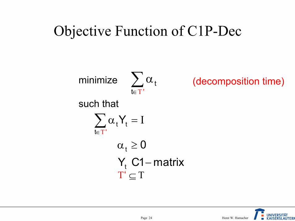
Objective Function of C1P-Dec
't t
t
t
t
Y
0Y C1 matrix
∈Τ
α = Ι
α ≥
−
∑
't
t∈Τ
α∑minimize
such that
Τ‘ ⊆ Τ
(decomposition time)

Horst W. HamacherPage 25
C1P-Dec is easy if T’=T
• C1P is separable into m independent row problems
• Each row problem is equivalent to min cost networkflow problem (solvable in linear time: O(mn))
Ahuja, Hamacher 2003
show transparencies

Horst W. HamacherPage 26
Bortfeld and Boyer (1993): Sweep algorithm
C1P-Dec is easy if T’=T

Horst W. HamacherPage 27
• No collision (interleaf motion) between adjacent leaf pairs
C1P-Dec with T’ ≠ T
• Minimal radiation width: dist > δ
dist

Horst W. HamacherPage 28
C1P-Dec with Technical Constraints
Boland, Hamacher, Lenzen, NETWORKS 2003“Minimizing Beam-On Time in Cancer Radiation Treatment
Using Multileaf Collimators”

Horst W. HamacherPage 29
yijt= 1 iff lit < j < rit (radiation)
Definition of Variables
lit ∈ {0,...,n} position of left leaf in row i
210 4 5 6
Row iat time t:
Column j
yijt = 0 0 1 1 1 0 03
lit=1 rit=5
Constraints: rit > lit+δ+1 (radiation width)ri+1,t > lit+1 and ri-1,t > lit+1 (interleaf motion)
rit ∈ {1,...,n+1} position of right leaf in row i

Horst W. HamacherPage 30
Path Representationof C1P
Graph G = (V,E) with
• nodes V = {(k,l,r) : r > l+δ+1, k = 1,...m, l = 0,...,n, r = 1,..,n+1}
101 102 103 112 113 123
201 202 203 212 213 223
301 302 303 312 313 323
401 402 403 412 413 423
• edges E satisfying interleaf motion constraints(k,l,r) → (k+1,p,q) if p ≤ r-1 and q ≥ l+1
• plus super source and super sink
x

Horst W. HamacherPage 31
Source-sink paths correspond to feasibleC1P matrices
101 102 103 112 113 123
201 202 203 212 213 223
301 302 303 312 313 323
401 402 403 412 413 423
0 1 2 3 D
D’
C1P-matrix network (with O(mn2) nodes)
=
1 00 11 11 0

Horst W. HamacherPage 32
Optimal C1P Decompositioncorresponds to minimal network flow
problem
sending αt units on path Pt ↔
use C1P matrix αt times
flow value↔
decomposition time
minimal flow value = minimal decomposition time

Horst W. HamacherPage 33
Example
=
+
23355223
10011110
2
01111001
3⇔
101 102 103 112 113 123
201 202 203 212 213 223
301 302 303 312 313 323
401 402 403 412 413 423
D
D’
α=3 α=2

Horst W. HamacherPage 34
D
D’
101 102 103 112 113 123
201 202 203 212 213 223
301 302 303 312 313 323
401 402 403 412 413 423
α=3 α=2
j=2
Example: I22=5i=2
∑ ∑ ∑−
=
+
+= ∈ −
=1
0
1
1 ),,(
j
l
n
jr rliEeije Ix
Constraint:
Which nodes contribute to Iij?

Horst W. HamacherPage 35
Consequence
∑ ∑ ∑−
=
+
+= ∈ −
=1
0
1
1 ),,(
j
l
n
jr rliEeije Ix
Minimum C1-Decomposition Time problembecomes a network flow problem
with side constraints
Polynomially solvable !

Horst W. HamacherPage 36
1 2 3 4 5 6 7 8 9 10 11 12 13 14 15Instances
Beam-On-Times of MLC

Horst W. HamacherPage 37
Integrality is important
T T 1
t ( t ) ( t 1)t 1 t 1
s−
σ σ += =
α +∑ ∑ minimize delivery time =beam-on time + set-up time
beam-on time
set-up time
back
sσ(t) σ(t+1) = constant set up time:T
tt 1
(T 1)=
α + −τ∑Minimizing T is NP hard (Burkard 2002)

Horst W. HamacherPage 38
Number of Shape Matrices
1 2 3 4 5 6 7 8 9 10 11 12 13 14 15
Instance
# M
atric
es

Horst W. HamacherPage 39
Delivery Time
1 2 3 4 5 6 7 8 9 10 11 12 13 14 15
Instance
Tota
l Del
iver
y Ti
me

Horst W. HamacherPage 40
irradiation arcs1371
0 1 2 3 4 5 6 7
1372 2581
How about integrality?
137
258
Side constraints are simpler as before:outfow copy1 = inflow copy2
Flow Model I Flow Model II

Horst W. HamacherPage 41
D
D’
1102
2102
1,0 1,1 1,2
2,0 2,1 2,2
1203 1213
2203 2213
3,0 3,1 3,2
4,0 4,1 4,2
1303
2302 23031402
2402
101 102 103 112 113 123
201 202 203 212 213 223
301 302 303 312 313 323
401 402 403 412 413 423
D
D’

Horst W. HamacherPage 42
101 102 103 112 113 123
201 202 203 212 213 223
301 302 303 312 313 323
401 402 403 412 413 423
D
D’
α=3 α=2
D
D’
1102 1113
2102 2113
1,0 1,1 1,2
2,0 2,1 2,2
1203 1213
2203 2213
3,0 3,1 3,2
4,0 4,1 4,2
1302 1303
2302 23031402 1413
24022413
α=3 α=2

Horst W. HamacherPage 43
Introduce lower = upper bound = Iij
on each irradiation arcfrom (i,j-1) to (i,j)!
3
5
2
2 5
3
3 2
=
3 22 55 33 2
I

Horst W. HamacherPage 44
Integral Solvability
Find flow with minimal value satisfyingcapacities and side constraintoutfow copy1 = inflow copy2
Solvable by negative “cycle” argument!
(Existence result - no combinatorial algorithm)

Horst W. HamacherPage 45
Find Algorithm with ImprovedComplexity
Idea:
Represent each possible left leaf and each possible right leaf asnode of a network (2(m(n+1)) many nodes)
Shape matrices = Paths in the network
Decomposition = Network flow
Algorithm of Baatar and Hamacher (2003)

Horst W. HamacherPage 46
Example of Baatar Network
1,1
4,1
1,1
2,1
2,1
3,1
3,1
4,1
1,2
4,2
1,2
2,2
2,2
3,2
3,2
4,2
1,3
4,3
1,3
2,3
2,3
3,3
3,3
4,3
potential left leaf position
potential left leaf position
potential left leaf position
potential left leaf position
in channel 1
in channel 2
in channel 3
in channel 4
potential right leaf position
potential right leaf position
potential right leaf position
potential right leaf position
nodes:

Horst W. HamacherPage 47
1,1
4,1
1,1
2,1
2,1
3,1
3,1
4,1
1,2
4,2
2,2
2,2
3,2
3,2
4,2
1,3
4,3
1,3
2,3
2,3
3,3
3,3
4,3
edges:
Example of Baatar Network
cells21
1 2 3
leaf positions
1,2

Horst W. HamacherPage 48
paths:
Example of Baatar Network1 2 3
leaf positions1,1
4,1
1,1
2,1
2,1
3,1
3,1
4,1
1,2
4,2
2,2
2,2
3,2
3,2
4,2
1,3
4,3
1,3
2,3
2,3
3,3
3,3
4,3
1,2
1 00 11 10 1
=

Horst W. HamacherPage 49
flows:
Example of Baatar Network
1,1
4,1
1,1
2,1
2,1
3,1
3,1
4,1
1,2
4,2
2,2
2,2
3,2
3,2
4,2
1,3
4,3
1,3
2,3
2,3
3,3
3,3
4,3
1,2
1 00 11 10 1
=
0 11 11 11 0
=

Horst W. HamacherPage 50
flows:
Flow ⇒ Intensity Matrix
1 00 1
21 10 1
=
0 11 1
31 11 0
+
1,1
4,1
1,1
2,1
2,1
3,1
3,1
4,1
1,2
4,2
2,2
2,2
3,2
3,2
4,2
1,3
4,3
1,3
2,3
2,3
3,3
3,3
4,3
1,2
2
22
2
2
2
2
3
3
3
33 3
3
3
2 33 55 53 2
=

Horst W. HamacherPage 51
Intensity Matrix ⇒ FlowInteger matrix I = (Iij) is given.
Compute for all i=1,...,m and all j=1,...n+1
, 1max{ ,0}iij j i jleft I I −= −
and
, 1 ,max{ ,0}ii i jj jri I Ight −= −
(with Ii0=Ii,n+1=0)

Horst W. HamacherPage 52
Intensity Matrix ⇒ Flow
3 22 55 33 2
, 1max{ ,0}iij j i jleft I I −= −
3 0 02 3 05 0 03 0 0
, 1 ,max{ ,0}ii i jj jri I Ight −= −
0 1 20 0 50 2 30 1 2
(3 2) = (2 5) = (5 3) = (3 2) =

Horst W. HamacherPage 53
Intensity Matrix ⇒ Flow
Result:Any MLC realization of a givenintensity matrix I can be writtenas flow in the Baatar networkwithsupply leftij+wijanddemand rightij+wijsatisfying additional sideconstraints forbidding interleafmotion.
1,1
4,1
1,1
2,1
2,1
3,1
3,1
4,1
1,2
4,2
1,2
2,2
2,2
3,2
3,2
4,2
1,3
4,3
1,3
2,3
2,3
3,3
3,3
4,3

Horst W. HamacherPage 54
Intensity Matrix ⇒ Flow
12
1,1 1,2 2
1 1, 1,2 2
1, ...,
1, ..., 1, 2, ...,
1, ..., 1, 2, ...,
min
( ),
( ) ( ),
( ) ( ),
0,
n
i ij ijj
k k
ij ij i i j ijj j
k k
i ij ij i j i jj j
ij
i m
i m k n
i m k n
Tsubject to
T left left w
right w left left w
left left w right w
w
=
+ += =
+ += =
∀ =
∀ = − =
∀ = − =
= + +
+ ≤ + +
+ + ≥ +
≥
∑
∑ ∑
∑ ∑1, ..., , 2, ...,
0
i m j n
T
∀ = =
≥

Horst W. HamacherPage 55
Intensity Matrix ⇒ Flow
Result: Minimizing ijj
w∑such that flow exists satisfying side constraintsyields minimal beam-on-time decomposition.
Solvable by a linear program with mn many variables!
• Solvable in polynomial time• Faster than Boland-Hamacher network flow approach

Horst W. HamacherPage 56
Modifications Including Set-UpTimes
minimize delivery time withconstant set-up time (i.e. sσ(t)σ(t+1) = const )
Use same approach with integer variables counting thenumber of shape matrices used.
T T 1
t ( t ) ( t 1)t 1 t 1
s−
σ σ += =
α +∑ ∑

Horst W. HamacherPage 57
Current Research
Modifications Including Set-UpTimes
minimize delivery time withsequence dependent set-up time
Use arc-path formulation of flow
T T 1
t ( t ) ( t 1)t 1 t 1
s−
σ σ += =
α +∑ ∑
Use sσ(t)σ(t+1) as data of a traveling salesman problem.

Horst W. HamacherPage 58
• Several subproblems of radiation therapy have beensuccessfully tackled
• choice of radiation angle• representative system of Pareto solutions• minimizing beam on time
Summary of Part I
• Several results are interesting independent of application• integer solvability of C1 decomposition• NP completeness of cardinality decomposition
• Lots of open problems, e.g.• integrated system (angles + intensity profiles + realization)• efficient algorithms for (constant and variable) set-up time

Horst W. HamacherPage 59
1 2 3 4 5 6 7 8 9 10 11 12 13 14 15
Instances
KL - Literature:
• Hamacher, H.W. and F. Lenzen, 2000:”A mixed integer programming approach to the multileaf collimator problem”,in Wolfgang Schlegel and T. Bortfeld (edts.) The use of Computers inRadiation Therapy, Springer
• Boland, N. , H.W. Hamacher, and F. Lenzen, 2002:“Minimizing beam-on time in cancer radiation treatment using multileafcollimators” NETWORKS
• Bataar, D. and Hamacher, H.W., 2002: “New models for multileafcollimators”, Report, Fachbereich Mathematik, Universität Kaiserslautern
Part II:Algorithms and NumericsOnline Treatment Planning - A Decision Support Toolshow transparencies