- 1 -

OPERATIONAL RISK ASSESSMENT FOR AIRSPACE PLANNING Karim Mehadhebi

Direction des Services de la Navigation Aérienne karim.mehadhebi@aviation-civile.gouv.fr

Toulouse, France

Abstract ICAO policy requires that States maintain an

acceptable level of safety in the provision of air traffic services (ATS). As a consequence, airspace planners have to adapt this high level safety requirement in the context of their specific operational environment, whenever they implement a new procedure. The main difficulty lies in the nature of the risk, which, over the years, has gradually switched from a technical risk (due to either a failure or a poor performance of technical equipment), to an operational risk .In other terms, although the performance of navigation and surveillance has drastically improved over the years, the level of safety (expressed in terms of fatal accidents per flying hours) has not followed the same evolution. One of the reasons is that, for some scenarios of operational errors, the accuracy of navigation contributes to increase the risk of collision, as we show in the sequel of this paper.

In this paper we span the current methodologies used for quantitative risk assessment, and we explain their limitations for modeling scenarios of operational errors. Then, we introduce a new methodology, supported by an analytical collision risk modeling together with a software implementation, and we present two applications of this methodology, one involving the assessment of the operational risk in a given part of the airspace, and another one for the detection of “hot spots”.

Collision risk modeling applied to airspace planning

In ICAO documentation, the reference of highest level regarding the use of collision risk models is the DOC 9689, Manual on Airspace Planning Methodology for the Determination of Separation Minima ([2]). In this document, the risk assessment determined by a collision risk model (CRM) is decomposed in two independent components. The first component represents the influence of the route network on the collision risk, in terms of “how often a pair of aircraft is likely to

fall into a given scenario of accident”. The second component, which depends on the performance capability of the environment, corresponds to the probability of collision associated to the pair of aircraft. It is within this second component that the aircraft navigation performance, the ground and airborne communication performance, and the surveillance performance are taken into account.

What kind of operational hazard can be modeled by current CRMs, and what kind of operational hazard can not? It is clear that CRMs currently introduced in Ref [2] are not sufficient for modeling all situations, as separation minima for radar surveillance clearly illustrate. Initially, separation minima could be derived from the position errors due to radar measurement, but as the number of radars was increasing and the accuracy was improving, it became clear that, although a multi-radar measurement could have a very good accuracy, separation minima could not be reduced accordingly. As for the connection between navigation performance and the resulting risk, the analysis of TCAS alerts has revealed that, in some occasions, the risk was increased by the navigational accuracy of the aircraft. For instance, if an aircraft climbs to a flight level for which it was not cleared, it is precisely its lateral accuracy which will cause a risk of collision with another aircraft on the same route at that flight level. Therefore, we see that navigational errors can contribute to the safety. However, in current CRMs, position errors due to navigation performance and surveillance error are considered similarly, and added into a total error.

An intuitive illustration of the modeling of collision risk in the CRMs of Ref [2] is shown in Figure 1, for two co-altitude aircraft on parallel routes. Aircraft are initially seen by the air traffic controller as separated, which may not be the case if we consider the inaccuracy of the surveillance. The risk of collision is the risk that the navigational errors lead both aircraft to reduce their relative distance until they eventually collide in a future time.

2

initial reported position

“Likelihood” of the collision in this location

Separation S

Figure 1: Modelling of collision risk in current CRMs

Justification of the current stochastic modeling of uncertainties

The modeling of position errors as a stochastic process is perfectly valid in environments where aircraft positions are not updated too frequently (as in procedural airspace, or in ADS-C). Actually, between two consecutive position reports, an aircraft is likely to deviate significantly from its assigned route, due to multiple causes (either technical or operational). Therefore, it is reasonable to model the deviation from the assigned route as a random quantity, whose “cone of uncertainty” is likely to vary with the time. Another situation where this model applies is when the surveillance uses onboard information. In radar surveillance for instance, the vertical position of the aircraft corresponds to the Mode C code. If this information is corrupted by a technical cause (problem in the altimetry system for instance), then the air traffic controller is unable to detect and to correct this error. The stochastic modeling allows to represent all kinds of evolution of this error in the course of time (such as a drift, for instance).

Limitation of the current modeling from the ATC’s viewpoint

With such a modeling, it is not easy to explain why an improved navigational performance can increase the risk of collision. The reason is that the deviations from the assigned route are modeled as “random excursions”, whereas in many cases of operational errors we know exactly what the deviation will be, without any need to use random modeling. In order to clarify this idea, we consider an environment like the French continental airspace, where, in multi-radar environment, positions are reported to the controller’s scope every 4 seconds (for two radars). The multi-radar processing makes the position fairly accurate, so

that the position displayed on the controller’s scope represents the actual position of the aircraft, corrupted by a small error due to the radar processing and the latency. This latency may also corrupt the speed vector, in the case, for instance, of a change of manoeuvre from the aircraft.

When aircraft positions are updated every four seconds, the modelling of random deviations shown in Figure 1 no longer applies, since the frequent updates does not allow aircraft to significantly deviate between consecutive position updates. In that case, we believe that the main cause for the risk of collision has to be sought in scenarios where the trajectory anticipation made by the ATC no longer corresponds to the reality of an aircraft trajectory. In the sequel of this paper, we will denote such scenarios of bad anticipation by the ATC as operational errors. In the vertical dimension, a typical scenario of operational error is the following: One aircraft is in vertical evolution, and the ATC expects this aircraft to level off at a given FL, but this aircraft keeps on climbing/descending. In the horizontal dimension, another typical scenario of operational error corresponds to the case where one aircraft is expected to turn, but keeps on in straight line. The two previous scenarios are denoted by “straight line” scenarios of operational error, in the sense that in both cases the aircraft follows its route in straight line, either in vertical or in horizontal dimension. We may also consider a “straight line” scenario for the speed, in the case of two aircraft flying one behind the other, and the ATC would instruct the queuing aircraft to reduce its speed, without being obeyed.

For such scenarios of operational errors, there is no benefit in adding random position errors to our modelling, as we now explain. Figure 2 shows such an example of operational scenario, where an aircraft keeps on climbing instead of leveling off at his cleared FL. In this situation, we know by advance that the trajectory for this scenario is roughly an extrapolation from the climbing phase of the aircraft. If we assume that the climbing aircraft and the steady aircraft are on the same horizontal route, then in case of an operational error the introduction of a lateral error will reduce the risk of collision. In other terms, it is precisely because aircraft have an excellent navigation accuracy that the operational error has higher chances to result in a collision. We see the difference with the paradigm of Figure 1, where the risk of collision was due to the introduction of position errors from the assigned routes. In scenarios of operational errors such as in Figure 2, the introduction of position errors tends to reduce the assessment of the risk.

3

In the RVSM safety assessment made by UK, different scenarios of operational errors have also been modeled in terms of deterministic trajectories (see Reference [3]).

FL

Real trajectories

Possible operational error

Figure 2: Deterministic trajectory for an operational error

It was found that the risk estimate given by this modeling was more conservative that another risk estimate based on the Reich model (see Ref [2] for a description of the Reich Model).

We believe that the modeling of scenarios of operational errors by deterministic trajectories often provides a satisfactory answer to the estimation of a collision risk induced by a scenario of operational hazard. For such a modeling, the risk is a consequence of the following factors:

1) What if the arrival time of the steady aircraft at the “vertical colliding point” had been slightly different?

2) How long would it take to the controller to detect this operational error?

3) What would be the chance for the controller to solve the operational error before the collision?

Before introducing our methodology, we now consider the limitations of another widely used safety assessment methodology, based on EUROCONTROL EATMP Safety Assessment Methodology.

Limitations of qualitative safety assessment methodologies

Introduction of the methodology The word “qualitative” refers to the fact that in this methodology the scenarios of operational errors are determined qualitatively, either by brainstorming or by operational experts. This differs from quantitative safety assessment methodologies such

as collision risk models, where the risk of collision is determined by stochastic modeling of random deviations.

FHA

Determination ofsafety objectives

PSSA

Derivation of riskmitigation strategy

SSA

Verification thatsafety requirements

have been met

Classified hazards and related safety objectives

Safety requirements

Hazards for numerical assessment

CRM

Figure 3: Architecture of qualitative safety assessment methodologies

Figure 3 shows the general architecture of this qualitative safety assessment methodology. Initially, a high level safety requirement is defined, similar to the acceptable level of safety defined in ICAO documentations. This safety requirement is often denoted as a Target Level of Safety (TLS). The purpose of the safety assessment methodology is to demonstrate that the current environment meets this TLS. Schematically, the demonstration is done in three consecutive steps:

1) The Functional Hazard Assessment (FHA) identifies potential operational hazards and assesses their effects on the safety of operations. It outputs the classified (in compliance with ESARR 4 severity classification scheme) hazards and their associated safety objectives. Operational hazards together with their severity are coupled together into fault trees with AND/OR gates.

2) Based on the TLS, The Preliminary System Safety Assessment (PSSA) determines the maximal frequency of occurrence of the operational hazards, in order to meet the TLS.

3) The SSA (System Safety Assessment) demonstrates that the current system meets the TLS, by checking that the frequency of occurrence of the operational hazards is not higher than the maximal rate determined in the PSSA.

In the architecture of Figure 3 we have also shown the connection between this qualitative methodology and the collision risk modeling methodology. If a given operational hazard can be modeled by a collision risk model, then it is possible to assess its severity in a more objective

4

way than with the FHA process. Actually, in a FHA, the severity is assessed by expert judgment.

Limitations of the methodology for assessing operational risk We now expose some limitations of this methodology for the assessment of operational risk. The first limitation stems from the classification of operational hazards made in the FHA. For all operational hazards identified in the FHA, a fixed severity has to be determined. However, in the real life, this severity depends on the underlying context. This context includes both the ATC (what was the ATC workload?) and the aircraft parameters. In addition, a parameter may have several effects, of opposite nature. For instance, in the case of the operational hazard illustrated in Figure 2 (a flight level overshoot), the fact that the climbing aircraft has a high climbing rate simultaneously reduces the intervention time for the controller, and the “crossing time” of the climbing aircraft when it crosses the FL of the steady aircraft.

In our opinion, the obligation to associate to all operational hazards a severity independent of the context is the major limitation of this methodology, and we will see in the sequel of this paper how our methodology has attempted to overcome this limitation.

Another limitation of the methodology has to do with the SSA step. The objective of the SSA is to check that the frequency of operational hazards in the current system is not higher than the “upper bound” value determined in the PSSA. This is done by processing all reported incidents. Now, if we consider a scenario of operational error consisting in a bad anticipation of the future trajectory of an aircraft (as our “straight line scenarios” previously introduced), this scenario will not necessarily result in an incident. For instance, a flight level overshoot similar to the one shown in Figure 2 may well be undetected if there was no other aircraft in the vicinity. Even if all incidents have been collected and analyzed, what is still missing is the probability for an operational hazard to result in an incident.In order to clarify this idea, we give a simple example. We suppose that, in a safety assessment, the PSSA has determined that the occurrence of flight level overshoots (similar to Figure 2) in a given area should not exceed 10 occurrences per year. We also suppose that in one year 4 incidents have been reported, due to a flight level overshoot. If the probability for a flight level overshoot to result in an incident is found to be equal to 1/3, then the expected number of flight level overshoots which occurred during the year can be estimated as

123/1

4 = , which is higher than the upper bound

value of 10.

Synthesis and introduction of our methodology The methodology that we now introduce has been designed in order to overcome the limitations explained in the previous section. We recall our definition of an operational error, which encompasses all scenarios where the anticipation made by the ATC does not correspond to the reality of the trajectory. This includes all “straight line” scenarios (the aircraft is expected by the controller to “do something” but he continues in straight line), but other operational scenarios can be considered, where the aircraft would deviate from its route. Such situations occur, for instance, when the ATC confuse two call signs, or when a pilot executes an ATC instruction which was issued to another aircraft.

The purpose of the methodology is to estimate the risk of collision resulting from a given scenario of operational error, and to better understand the connection between this risk and the underlying environment. Our methodology is supported by a stochastic modeling of the risk induced by a given operational error, and it has been implemented into a software. We firstly introduce our stochastic modeling, and then we present the current software implementation.

Stochastic modeling of the risk induced by an operational error

Until now, only the “straight line” scenarios have been implemented in our stochastic modeling. They represent by far the most frequent occurrences of operational error (particularly in the vertical dimension).

«Straight line» trajectory modification :the deviating aircraft follows hisroute:

– in the horizontal plane

– or in the vertical dimension

Figure 4:”straight line” scenarios of operational error

5

For both scenarios, we assume that the horizontal or vertical maneuver made by the aircraft was due to a loss of separation with the neighboring aircraft.

FL

time t

∆tp

∆z

∆tp ∆tc

Figure 5: modeling of time uncertainties

Our modeling of uncertainties is time oriented rather than position error oriented. We mean that, instead of inserting position errors as in current CRMs, we assume that an aircraft flying along its trajectory could have arrived at a given point slightly earlier or later. We also assume that an aircraft cleared to change its FL could as well have started its vertical evolution slightly earlier or later. Figure 5 illustrates our modeling. The along track error (corresponding to a delay or an anticipation) is denoted by pt∆ . The uncertainty on the starting

time of a vertical evolution is denoted by ct∆ . The magnitude of these errors is determined by the current separation in the airspace.

For two aircraft flying in straight line with a crossing angle denoted byθ , a quick computation shows that the minimal horizontal distance for the pair of aircraft is given by

θ

θ

cos2

sin

212

22

1

2121min

VVVV

VVttD hh

−+−= (1)

where 1ht and 2ht are the two times of arrival at the crossing point. Therefore, in our methodology, we assume that the difference between the time of arrival of both aircraft at the crossing point follows a uniform distribution on the interval [ ]pp TT ∆∆− , with

hor21

212

22

1 Sepsin

cos2θ

θVV

VVVVTp

−+=∆ (2)

And horSep is the value of the horizontal separation. Our modeling means that, relatively to one aircraft, the other aircraft could have arrived at the crossing point slightly earlier or later, provided that both aircraft were in the course of losing their horizontal separation. This results from our previous assumption that the maneuver instructed

by the ATC was due to the fact that the maneuvering aircraft was in the course of a loss of separation with another aircraft.

Similarly, we see on Figure 5 that the uncertainty

ct∆ induces, at a fixed time, a vertical uncertainty

z∆ with cz tvz ∆×=∆ , where zv is the vertical speed. This suffices to determine the magnitude of the uncertainty ct∆ in order to guarantee that the pair of aircraft will pass vertically within the vertical separation vertSep . In conclusion, we assume that, for each aircraft, the time uncertainty

ct∆ is uniformly distributed on an interval

[ ]cc TT ∆∆− , where the value of cT∆ is chosen so as to verify that both aircraft will vertically pass within a vertical distance below vertSep . The rational is similar to the horizontal case: we assume that the maneuver was due to a conflict solving from the controller from a proximate loss of separation.

We now give, for the pair of aircraft, the associated probability of collision, in the simplified case where both aircraft follow a straight line route, with a crossing angle denoted byθ . We have not provided any analytical derivation due to the limitation on the length of the paper, but the reader interested by it can either ask it by email to the author or read Reference [5].

The two aircraft are modeled by cylinders, whose diameter is denoted by xyλ and whose height is

denoted by zλ . The collision corresponds to the intersection of the two cylinders. In the case when the two aircraft fly in straight line, the probability of collision for the pair of aircraft differs whether one or two aircraft are in vertical evolution.

In the case when the two aircraft are in vertical evolution, the probability of collision is given by

{ }

2

2with

)(21

δV2

V2sinV

collisionPr

1,2,

2,2

1,2,

1,1

21zrel21

rel

∆−

=

∆−

=

+

+

∆==

c

zz

z

c

zz

z

zxy

p

xy

Tvv

va

Tvv

va

aaTVVλπλ

θλ

(3)

Where the relative horizontal speed is given by

θcos2V 212

22

1rel VVVV −+= , the relative

vertical speed is given by zδV , and the vertical

speed of the two aircraft are given by 1,zv and

2,zv .

6

If one aircraft is in vertical evolution and the second one is steady, the probability of collision is given by

{ }c

zxy

p

xy

TTVV ∆

+

∆= zrel

21

rel δV2

V2sin

VcollisionPr

λπλ

θλ (4)

We have added to our model a probability for the controller to detect and to solve the conflict. The probability for the controller to solve the conflict is a function of the available time. If the air traffic controller has less than impt , then he does not have sufficient time to solve the conflict. If he has more than post , then he can solve the conflict. Between these two values, the distribution function is interpolated linearly, as shown in Figure 6. The detection time of the controller has been modeled as a positive random variable with an exponential distribution. The justification for this choice of distribution is given in Appendix A.

solveP

impt post

1

0

Figure 6: probability to solve the operational error as a function of the available time

If we denote by λ the parameter of the exponential distribution, we find that the probability for the controller to detect and solve the operational error is a function of the available time before the collision, denoted by collisionT . This probability,

denoted by , ATCP is given by :

If impcollision tT < , 0=ATCP .

If poscollisionimp tTt ≤< ,( ) ( )

( )λλλ

imppos

impcollisiontT

ATC tttTe

Pimpcollision

−−+−

=−− 1

If collisionpos Tt ≤ ,( ) ( ) ( )

( )λλλλ

imppos

imppostttT

ATC ttttee

Pimpposimpcollision

−

−+−=

−−−−

Finally, the probability of collision is given by

{ } ( )ATCP−× 1collisionPr (5)

When the pairs of aircraft are extracted from real radar data, the situation is often more complex, since one or the two aircraft may not fly in straight line. Nevertheless, the probabilistic modeling can be extended to these cases by following the same approach.

Software implementation The software takes as inputs files of collected

radar data, and determines the encounters of aircraft likely to result in an operational error, either in vertical or in horizontal. Before introducing the applications of the software for safety studies, we introduce the general methodology for processing radar data. A typical application of the software involves the following tasks, which are done in sequence.

Smoothing of radar data. Each aircraft trajectory is smoothed individually, and aircraft positions are determined with a fixed time, generally of 5 seconds. In addition to this, the horizontal and vertical maneuvers of the aircraft are detected.

Detection of encounters. After the previous step, the collected radar data consists of synchronous aircraft positions (usually one position every 5 seconds). Then, the whole traffic is played, and pairs of aircraft likely to result in an operational error are identified as encounters. For each encounter, the software stores a certain duration of the trajectory before and after the change of maneuver. All this can be tuned by the user.

Post processing of the encounters. Then, each encounter is processed a second time. Actually, it is impossible to interpret the scenario of operational error by playing the traffic in “real time”, this is why the interpretation of the operational error is done afterwards. During this post processing, all encounters which do not correspond to the horizontal or vertical straight line scenario are discarded.

Edition of the encounters. Finally, the encounters which are determined are stored into a file with a special format. These files can be opened by our software, and the conflicts can be edited and visualized.

Smoothing of radar data The algorithm use weighted roughness spline functions, which are smoothing function whose rigidity can be set locally (see Ref [4]). The principle of the algorithm is to smooth each trajectory twice. After the first smoothing, the rogue points are identified and excluded, and the

7

maneuvers are detected. Then, the rigidity of the smoother is set at a high level in the “straight line” portions of the trajectory, and at a low level in the maneuvers. The trajectory is then smoothed a second time, with the values of the rigidity of the spline defined previously.

Figure 7 illustrates the HMI of the smoother. The user can refine the choice of the parameters for the smoother, and edit all trajectories in a two-view panel, enabling to observe simultaneously joint parameters. In Figure 7, we see on a top view the X/Y trajectory of the aircraft, and on the bottom view the corresponding heading. The blue bullet indicates the position of the aircraft on each curve. The parameters are selected in order to make the change of heading as abrupt as possible, without anticipation or delay in the value of the heading .

Figure 7: Detection of a turn

Figure 8 shows, on the top view, the vertical profile of the trajectory (time in horizontal, and FL in vertical), whereas the bottom view shows the speed profile (time in horizontal, and speed in vertical). We see that the speed change due to the climbing phase is well detected. The yellow points on the bottom view represent the speed estimation made by the local radar tracking, whereas the red curve shows the speed profile determined by the software once the maneuvers on speed have been determined.

Aircraft position

Figure 8: Detection of speed maneuver

Edition of the encounters The encounters determined in the detection and the post-processing phase are then stored into a file. This file can be opened by our software, and the encounters can be classified, sorted, and played. Figure 9 shows the panel editor for the encounters. This panel allows to play the encounter, and to check the validity of our modeling of the operational error.

Vertical view

Horizontal view

Current flight parameters

Current conflict parameters

Conflictfields todisplay

Displayedfields

Time slider

Current aircraft positions

Figure 9: Edition panel for the encounters

The operational scenario of error (in the case of Figure 9, a flight level overshoot) is represented by a blue bullet. The aircraft trajectory corresponding to the scenario of operational error is also represented by a red segment.

We now present the scenarios of operational errors currently implemented in the software.

Scenarios of operational errors There are currently 8 scenarios of operational

errors processed by the software, all corresponding to “straight line” scenarios, either in the horizontal, the vertical or the speed dimension. We illustrate below two scenarios, one in vertical and one in horizontal The crossing points are represented by big bullets. The red crossing point corresponds to the actual crossing, whereas the blue bullet corresponds to the location of the crossing in the case of the operational error.

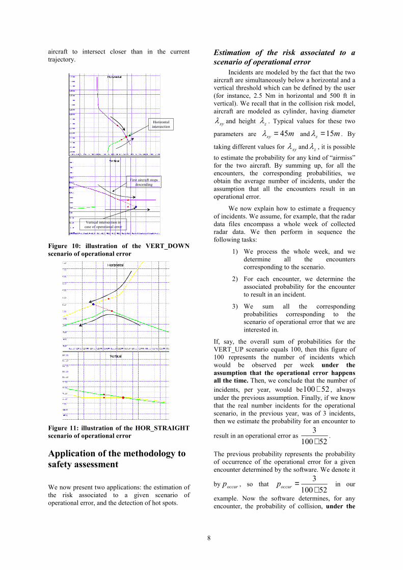
The scenario of operational error, denoted by VERT_DOWN, applies to an encounter where one aircraft is steady at a flight level, and the other aircraft descends and stabilizes at an upper flight level. An example is given in Figure 10. The trajectories cross in the horizontal plane.

The scenario of operational error illustrated on Figure 11, denoted by HOR_STRAIGHT, applies to situations where both aircraft trajectories intersect in horizontal. The operational error corresponds to a situation where one aircraft does not turn and goes in straight line, causing both

8

aircraft to intersect closer than in the current trajectory.

First aircraft stops descending

Horizontal intersection

Vertical intersection in case of operational error

Figure 10: illustration of the VERT_DOWN scenario of operational error

Figure 11: illustration of the HOR_STRAIGHT scenario of operational error

Application of the methodology to safety assessment

We now present two applications: the estimation of the risk associated to a given scenario of operational error, and the detection of hot spots.

Estimation of the risk associated to a scenario of operational error

Incidents are modeled by the fact that the two aircraft are simultaneously below a horizontal and a vertical threshold which can be defined by the user (for instance, 2.5 Nm in horizontal and 500 ft in vertical). We recall that in the collision risk model, aircraft are modeled as cylinder, having diameter

xyλ and height zλ . Typical values for these two

parameters are mxy 45=λ and mz 15=λ . By

taking different values for xyλ and zλ , it is possible to estimate the probability for any kind of “airmiss” for the two aircraft. By summing up, for all the encounters, the corresponding probabilities, we obtain the average number of incidents, under the assumption that all the encounters result in an operational error.

We now explain how to estimate a frequency of incidents. We assume, for example, that the radar data files encompass a whole week of collected radar data. We then perform in sequence the following tasks:

1) We process the whole week, and we determine all the encounters corresponding to the scenario.

2) For each encounter, we determine the associated probability for the encounter to result in an incident.

3) We sum all the corresponding probabilities corresponding to the scenario of operational error that we are interested in.

If, say, the overall sum of probabilities for the VERT_UP scenario equals 100, then this figure of 100 represents the number of incidents which would be observed per week under the assumption that the operational error happens all the time. Then, we conclude that the number of incidents, per year, would be 52100× , always under the previous assumption. Finally, if we know that the real number incidents for the operational scenario, in the previous year, was of 3 incidents, then we estimate the probability for an encounter to

result in an operational error as 52100

3×

.

The previous probability represents the probability of occurrence of the operational error for a given encounter determined by the software. We denote it

by occurp , so that 52100

3×

=occurp in our

example. Now the software determines, for any encounter, the probability of collision, under the

9

assumption that the corresponding operational error happens for the encounter. We denote this latter probability by encounterp . We have seen in the previous subsection how to determine the probability of occurrence of the operational error for a given encounter. We deduce that the probability of collision for the encounter, collisionp ,

is given by encounteroccurcollision ppp ×= . By

summing up all the collisionp for all the encounters determined during the week of collected data, we find a expected number of collisions, that we denote by collisionN . Finally, we determine the total

flying time over the week, that we denote by flyT ,and the risk, expressed in terms of number of

collision per flying hour, is given by fly

collision

TN

.

Detection of “hot spots” The second application is the detection of “hot spots”. Once the encounters have been determined, it is possible to display them geographically, as shown in Figure 12, together with the trajectories of steady aircraft. The green encounters correspond to scenarios of operational error in vertical, whereas the red/pink ones correspond to scenarios of operational errors in horizontal.

Figure 12: All encounters for one day of collected traffic

We see that most encounters correspond to vertical scenarios, and the link between the routes and the encounters becomes apparent. If we retain among the previous encounters those where the time available before the collision was below 40 seconds, we obtain the following Figure.

Figure 13: subset of encounters where the “time before collision was lower than 40 seconds

We see that most of these encounters are focused on a specific area and that in this specific area most of the encounters are still scenarios of operational errors in vertical. It is also possible to display parameters associated to a selection of encounters. For instance, having selected the encounters in the dotted oval of Figure 13, we represent them on Figure 14 by a two dimensional diagram showing the FL (in vertical) and the time before collision (TCOL) in horizontal:

Figure 14: two dimensional display of the encounters

We see that most of these encounters occur between FL250 and FL350.

Further work The methodology presented in this paper is

still in evolution. We plan, in the future, to add detection and interpretation of the instructions given by the ATC, by including into the methodology the flight plan information, and by detecting and interpreting all deviations from the flight plan route. This would allow to characterize not only the operational risk, but also to model the ATC “cognitive workload”, in terms of number of encounters, stress associated to the encounters depending on their gravity, and so on.

10

References [1] Air Traffic Management, ICAO Doc

4444/ATM/501, 2001

[2] Manual on Airspace Planning Methodology for the Determination of Separation Minima, ICAO Doc 9689, 1998

[3] Marcus Dacre, Estimating Collision Risk for UK RVSM, ICAO SASP-WG/WHL/1-WP/24

[4] Carl De Boor, Calculation of the Smoothing Spline with Weighted Roughness Measure (1998), manuscript can be obtained at http://www.cs.wisc.edu/ deboor/ftpreadme.html (Madison)

[5] Karim Mehadhebi, Presentation and Software Implementation of a 3D CRM, Eurocontrol MDG/30-DP/02

Appendix In this appendix we justify our choice of an exponential distribution of the ATC detection time, using the hazard rate concept drawn from survival analysis. Any positive random variable T can be seen as a life duration. A realization of T becomes the life duration of a given individual among a population. Now, the conditional probability for an individual to die between t and t+1 day, given that he has survived until time t, is denoted in survival analysis as the hazard rate. If we denote it by

)(tλ , it is defined analytically by

( ) { }dt

tTtTdttt dt

≥≥>+= →

Prlim 0λ

If we denote by { }tTtF >= Pr)( the survival function of T, the previous Equation becomes

( )( ) ( )

)()('

)(lim 0

tFtF

dttF

tFdttF

t dt

=

−+

= →λ

And by integration and using the fact that { } 1)0(0Pr ==> FT we finally find that

∫=

−t

duu

etF 0

)(

)(λ

(6)

In our case, we have to model a human behavior of non detection of an unexpected deviation from an aircraft. We want to determine the probability density function of the duration time for the

controller to detect that an aircraft has deviated from its cleared route.

If we give to our hazard rate an increasing shape, it means that the longer the operational error has been lasting, the more chances the controller has to finally detect it. This is the case for normal operation, when the controller routinely checks its scope. A decreasing shape for our hazard rate would be overly pessimistic, meaning that if the controller has not detected quickly the operational error, he has less and less chances to detect it over the time. A good modeling of a human error is to take a constant rate, meaning that it is not because the controller has not detected the operational error over T seconds that he is more likely to detect it in the next second. Taking λ constant in Equation (6) gives )exp()( ttF λ−= , which is the survival function of an exponential distribution.

Author Biography Karim Mehadhebi graduated from Ecole

Polytechnique. He holds a MSc in Artificial Intelligence from Université Paul Sabatier (Toulouse) and a MSc in Computer Science from Mc Gill University (Montreal). His main activity is the design and implementation of software in fields involving both mathematical and algorithmic expertise, such as radar trajectory smoothing by spline techniques, radar bias tuning by generalized regression, and risk assessment by designing and implementing collision risk models. He represents DSNA within the ICAO SASP (Separation and Airspace Safety Panel) and has contributed to the work of the Eurocontrol MDG (Mathematics Drafting Group).