Operational Performance of Centrifugal Pumps

7/18/2019 Operational Performance of Centrifugal Pumps

http://slidepdf.com/reader/full/operational-performance-of-centrifugal-pumps 1/37

49

2 Operational performance of centrifugal pumps

2.1 Characteristic curves

2.1.1 Pump characteristic curves

For a centrifugal pump driven at constant rotational speed, the head H , the powerabsorbed P and hence the efficiency - as well as the ( NPSHR), are functions of theflowrate Q. The relationship between these different values is represented bycharacteristic curves. Fig. 2.01 shows an example of four characteristic curves of asingle stage centrifugal pump at a rotational speed n = 1450 rpm.

Fig. 2.01 Characteristic curves of a single stage centrifugal pump.

© Sterling Fluid Systems B.V



50

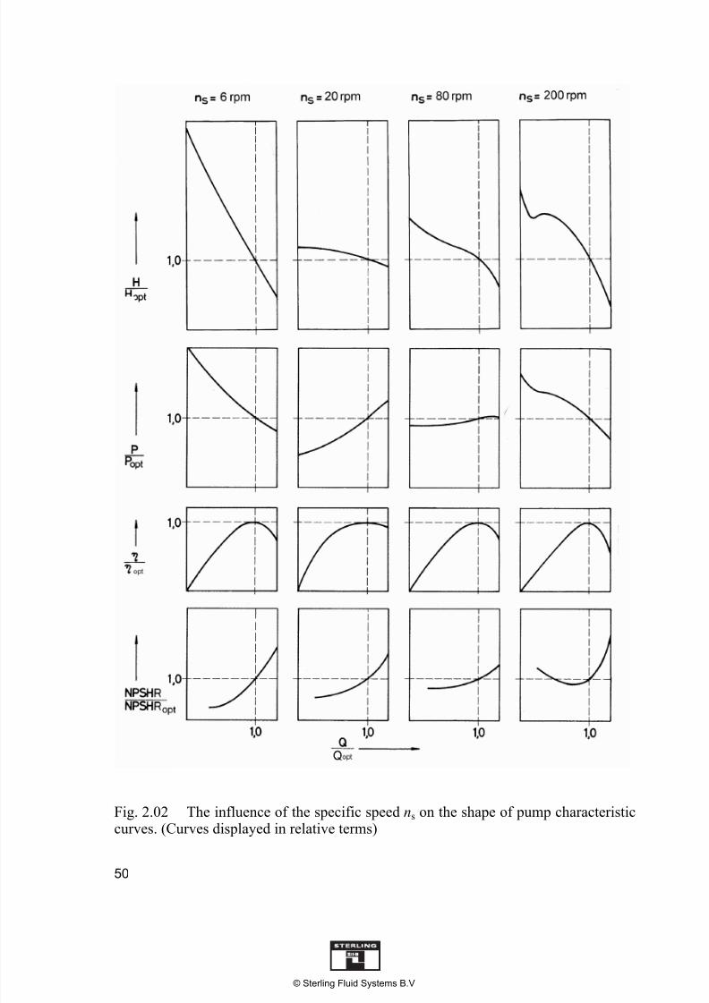
Fig. 2.02 The influence of the specific speed ns on the shape of pump characteristiccurves. (Curves displayed in relative terms)




51

The Head / Capacity curve H(Q) also known as the throttling curve - represents therelationship between the head of a centrifugal pump and its flowrate.

Generally the head decreases with increasing flowrate. The measure of this fall inhead is given in practice by the ratio:

H 0 – H opt

————— H opt

this is often termed the ‘steepness’.

This steepness ratio is a function of the specific speed and its values are:

for side channel pumps approx. 1 to 3

for radial flow pumps approx. 0,10 to 0,25

for mixed flow pumps approx. 0,25 to 0,80

for axial flow pumps over 0,80

The steepness ratio is therefore dependent on the type of pump and the shape of theimpeller and cannot be selected arbitrarily.

H(Q) curves in which the head decreases with increasing flowrate are described asstable. (Fig. 2.03a, b and c). With stable H(Q) curves, for each value of head thereexists only a single value of flowrate.

In contrast, an unstable H(Q) curve is one in which there is a range of flowrates forwhich the head increases with increasing flowrate. (Fig. 2.03d and e). With anunstable H(Q) curve there may be two or more values of flowrate for each value ofhead. The peak values on an unstable curve are known as Qsch and H sch. The shape ofthe characteristic curve in Fig. 2.03e is typical for pumps with high specific speeds,above ns 110 rpm.

Fig. 2.03

Typical characteristic H(Q) curves for centrifugal pumps.




53

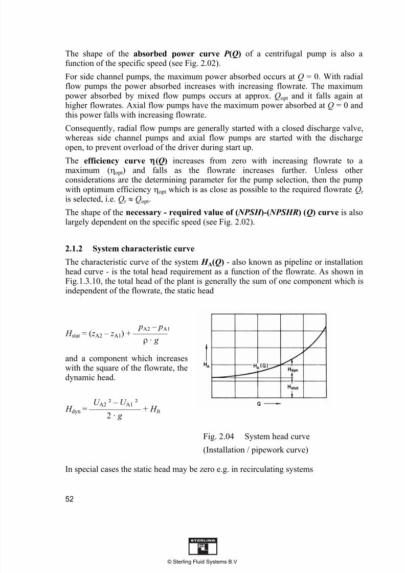
2.1.3 Interaction between the pump and system

The duty point of a pump is where the total head generated by the pump is equal tothe head required by the installation. In other words where the pump characteristic H (Q) and the system characteristic H A(Q) intersect.

This gives the flowrate Q, which the pump delivers through the system and thecorresponding values of absorbed power P , the efficiency and the necessary( NPSH )-value of the pump ( NPSHR). An important precondition for the operation atthe duty point is the requirement laid down in chapter 1.5.4, that the available( NPSH )-value of the installation ( NPSHA) exceeds the necessary ( NPSH )-value of the pump ( NPSHR) by at least the safety margin.

As a rule the selection of the pump is determined by the flowrate required; the totalhead of the system (= head of the pump) is then calculated to suit the specifiedoperating conditions.

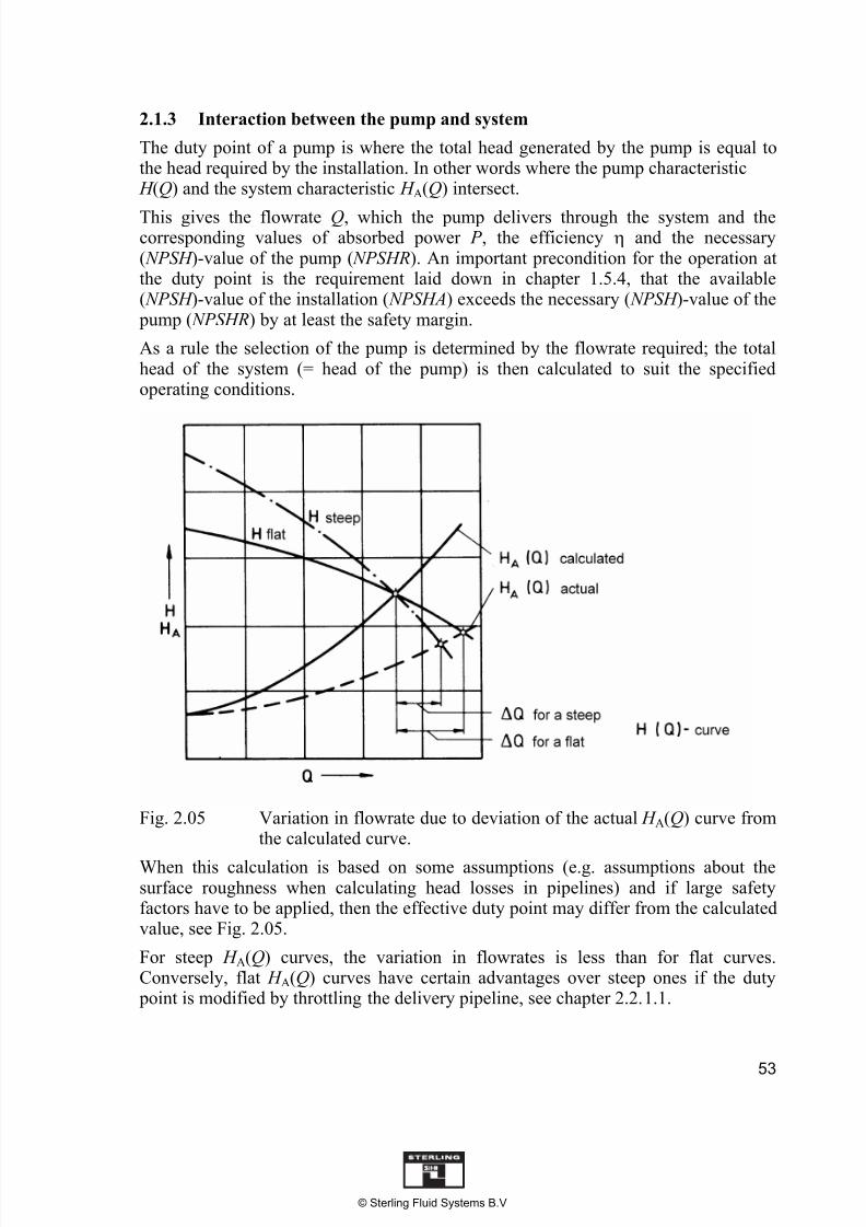
Fig. 2.05 Variation in flowrate due to deviation of the actual H A(Q) curve fromthe calculated curve.

When this calculation is based on some assumptions (e.g. assumptions about thesurface roughness when calculating head losses in pipelines) and if large safetyfactors have to be applied, then the effective duty point may differ from the calculatedvalue, see Fig. 2.05.

For steep H A(Q) curves, the variation in flowrates is less than for flat curves.Conversely, flat H A(Q) curves have certain advantages over steep ones if the duty point is modified by throttling the delivery pipeline, see chapter 2.2.1.1.




54

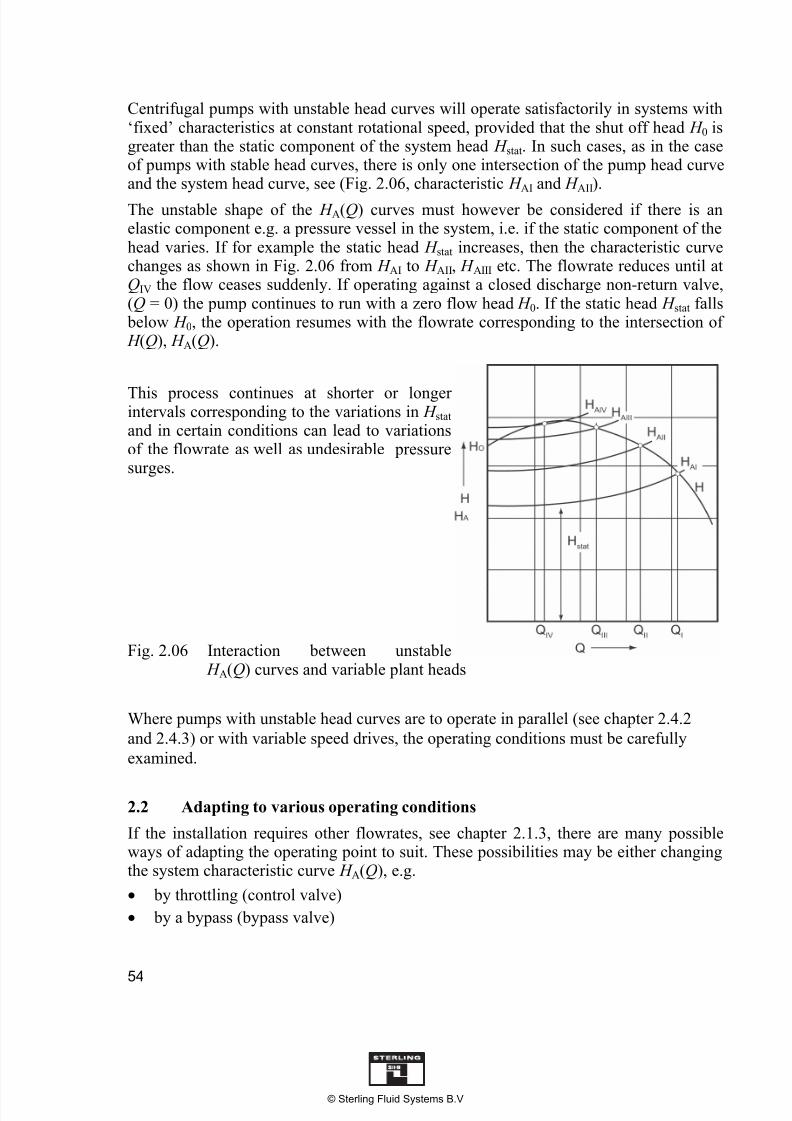
Centrifugal pumps with unstable head curves will operate satisfactorily in systems with‘fixed’ characteristics at constant rotational speed, provided that the shut off head H 0 isgreater than the static component of the system head H stat. In such cases, as in the caseof pumps with stable head curves, there is only one intersection of the pump head curveand the system head curve, see (Fig. 2.06, characteristic H AI and H AII).

The unstable shape of the H A(Q) curves must however be considered if there is anelastic component e.g. a pressure vessel in the system, i.e. if the static component of thehead varies. If for example the static head H stat increases, then the characteristic curvechanges as shown in Fig. 2.06 from H AI to H AII, H AIII etc. The flowrate reduces until atQIV the flow ceases suddenly. If operating against a closed discharge non-return valve,(Q = 0) the pump continues to run with a zero flow head H 0. If the static head H stat falls below H 0, the operation resumes with the flowrate corresponding to the intersection of H (Q), H A(Q).

This process continues at shorter or longerintervals corresponding to the variations in H stat

and in certain conditions can lead to variationsof the flowrate as well as undesirable pressuresurges.

Fig. 2.06 Interaction between unstable H A(Q) curves and variable plant heads

Where pumps with unstable head curves are to operate in parallel (see chapter 2.4.2

and 2.4.3) or with variable speed drives, the operating conditions must be carefully

examined.

2.2 Adapting to various operating conditions

If the installation requires other flowrates, see chapter 2.1.3, there are many possibleways of adapting the operating point to suit. These possibilities may be either changingthe system characteristic curve H A(Q), e.g.

by throttling (control valve)

by a bypass (bypass valve)




55

On changes to the pump characteristic curve H (Q), e.g.

by changing the impeller diameter

by undercutting the angle of the blade tips

by fitting dummy stages

by speed variation

(speed control / adjustment)

by adjusting the angle of inlet guide vanes upstream of the impeller (pre-swirl)

by creating pre-swirl immediately upstream of the impeller by means of adirectional bypass flow (bypass pre-swirl)

by adjusting the angle of incidence of the blades (pitch adjustment)

2.2.1 Adjusting the system characteristic

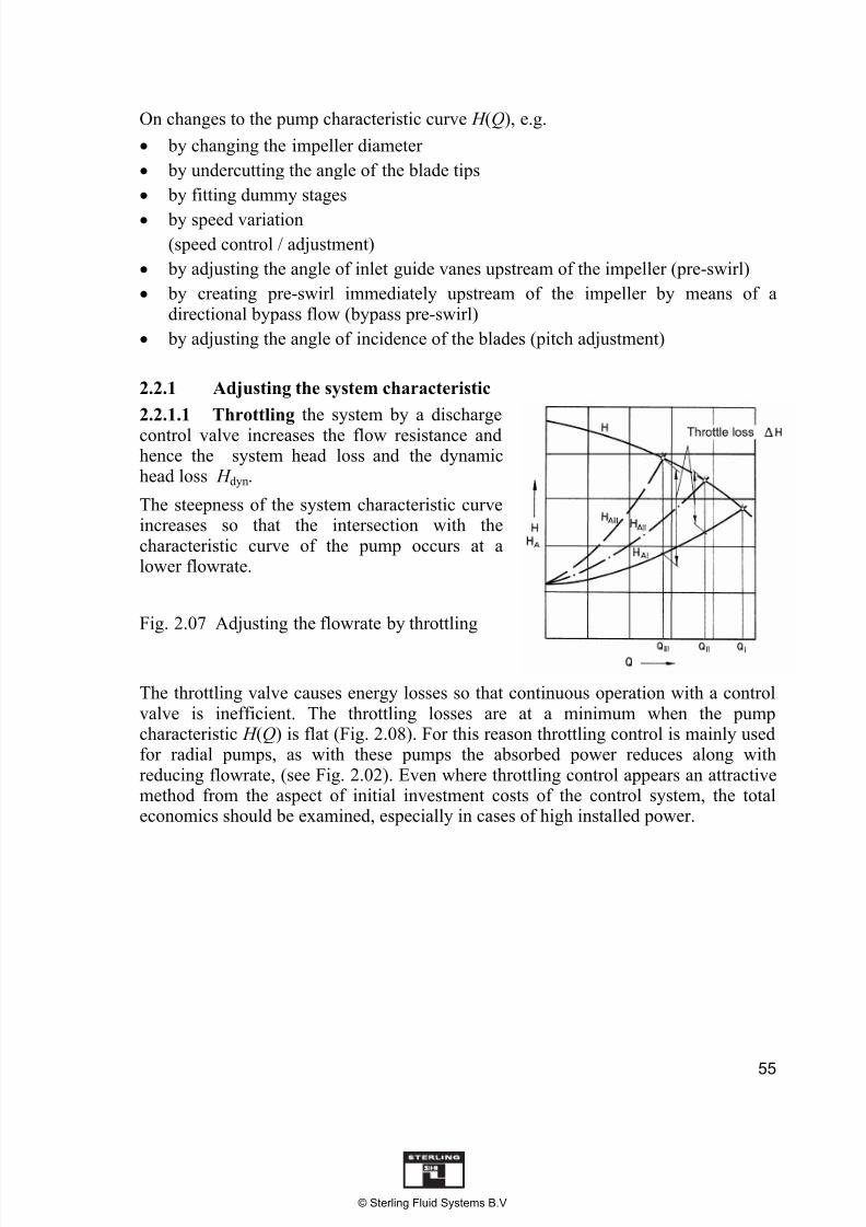
2.2.1.1 Throttling the system by a discharge

control valve increases the flow resistance andhence the system head loss and the dynamichead loss H dyn.

The steepness of the system characteristic curveincreases so that the intersection with thecharacteristic curve of the pump occurs at alower flowrate.

Fig. 2.07 Adjusting the flowrate by throttling

The throttling valve causes energy losses so that continuous operation with a controlvalve is inefficient. The throttling losses are at a minimum when the pumpcharacteristic H (Q) is flat (Fig. 2.08). For this reason throttling control is mainly usedfor radial pumps, as with these pumps the absorbed power reduces along withreducing flowrate, (see Fig. 2.02). Even where throttling control appears an attractivemethod from the aspect of initial investment costs of the control system, the totaleconomics should be examined, especially in cases of high installed power.




56

Fig. 2.08 Throttling losses for steep and flat H (Q) curves

For side channel pumps, mixed flow pumps from ns 100 rpm and for axial flow pumps, it should be remembered that the power absorbed increases with decreasingflowrate. In addition axial flow pumps may move into a range of unstable operationdue to the throttling process. This means rough running and an increased noise level, both being features of pumps with high specific speed, so this range of operation is to be avoided for continuous operation.

Fundamentally, throttling should always be done on the delivery side of the pump.Throttling the suction side of the pump will cause a reduction in available ( NPSH )value of the system ( NPSHA), (see chapter 1.5.4 ) and must be avoided due tocavitation danger.

2.2.1.2 With Bypass control a recirculation line, parallel to the pump, returns part ofthe flow from the delivery side of the pump to the suction side. Dependent on thecharacteristic of the bypass curve, the characteristic curve of the system increases to alarger flowrate.

Qges = QBypass + QA (Fig. 2.09)

As a result the flowrate of the pump increases from QI to Qges, and the net useful flowthrough the system decreases from QI to QA.




57

In the case of a high bypass flow, to preventexcessive warming of the pumped liquid, the

recirculation should be returned to thesuction vessel, not the pump suction pipe.

Fig. 2.09 Flow control by means of a bypass

Flowrate control by means of a bypass is especially recommended for side channeland axial flow pumps, as the power absorbed by the pump decreases with increasingflowrate.

2.2.2 Adjustment of pump characteristic

2.2.2.1 The reduction of impeller diameter is a useful method of permanentlyreducing the flowrate and total head of the pump.

Impeller trim is only possible however with radial flow and to a limited extent, mixedflow impellers. In the case of pumps without a diffuser e.g. volute case pumps, thediameter of the impeller is reduced by machining the diameter D down to Dx, in thecase of pumps with a diffuser e.g. multistage split case pumps, the impeller is usuallymodified by machining down the vanes only to diameter Dx , as shown in Fig.2.10.

Fig.2.10 Reduction of impeller diameter.




58

If only a minor adjustment is made to the impeller or vane diameter the followingrelationships apply to the flowrate and head:

Qx / Q = ( Dx / D)²

H x / H = ( Dx / D)²

The diameter Dx can be established for the usual linear co-ordinates of the H /(Q)characteristic from the following curves (Fig 2.11):

Draw a straight line through the point Q = 0, H = 0 and the desiredduty point Qx , H x ; this lineintersects the H (Q) curve of theunmodified impeller at point “S”.Using the values of Q and H of this point the diameter Dx can becalculated from:

Dx D · (Qx / Q)0,5

or

Dx D · ( H x / H )0,5

Fig. 2.11 Modifying pump performance by reduction of impeller diameter

The above calculations are not accurate if the performance of the pump needs to bereduced by a large amount and it is recommended that adjustments are made insmall steps.

Initially the impeller should be reduced to a diameter larger than the calculated figure Dx, and the pump then tested to determine the final required diameter. For pumps ofhigher performance this final diameter may need to be established in several steps.

In order to avoid this expensive procedure for pumps which are manufactured inquantity, standard design data such as measured curves for H (Q), P (Q) and (Q) iscollated, not only for the unmodified impeller diameter D but also for severalimpeller trims Dx . This data is often presented in the form of contour curves. In this

way the above relationships can also be used for substantial diameter reductions byinterpolating between values for different impeller diameters.

For pumps with low specific speed, the loss of efficiency for minor impelleradjustments is small, but pumps with higher specific speed and hence pumps withmixed flow impellers display a noticeable drop in efficiency, even for smalladjustments.




59

Fig. 2.12

H (Q) Characteristic curves for a single stage volute casing pump for maximum,minimum and intermediate impeller diameters.

For multistage ring section pumps the adjustment of operating characteristics can beachieved by a combination of impellers with different diameters. For each size of pump there is a combination of impeller diameters and number of stages which givesa narrow field of different characteristics, without the need for expensive and timeconsuming impeller diameter adjustments.

This method does not always ensure exactly matching the selection point (Q and H ).It is therefore possible that depending on the characteristic, the flowrate may be largerthan required. As a result the total head and power absorbed will rise. Therefore thismethod should only be used for powers up to approx. 50 kW. For larger powers theefficiency should be checked.

If a combination of different impellers is not applicable, then all the impellers aretrimmed to the same diameter.

So that the ( NPSH3) value is not affected, the first stage impeller is not trimmed.




60

Fig. 2.13

H (Q) Characteristics for multistage ring section pumps with variousimpeller combinations

The impellers of waste water pumps (paddle wheel impellers) and slurry pumpscannot have impeller diameter trims for hydraulic reasons. For these types of pumpsthe characteristics are adjusted by speed control (see chapter 2.2.2.4 ).

Impeller adjustment is also not possible for tubular case pumps with axial or mixedflow impellers. Any necessary adjustment is made by an alteration of the blade anglesor guide vane angle and/or selection of motor with appropriate speed or withintermediate gearbox. Similarly side channel pumps are not suitable for impellertrimming.

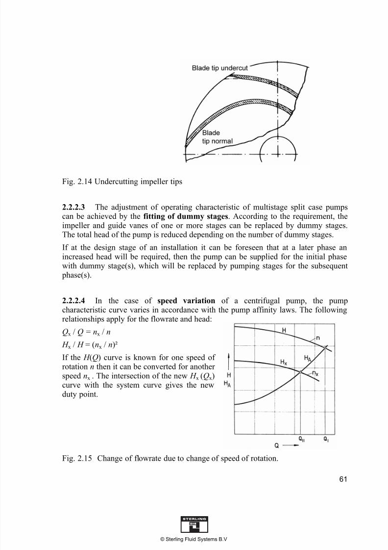
2.2.2.2 The undercutting of the angle of blade tips is a means of achieving smallincreases in the total head generated by centrifugal pumps with radial or mixed flowimpellers. In the range of optimum flowrate the H (Q) characteristic can be raised byapproximately 3%. The undercutting has little effect on the shut off head H 0.




61

Fig. 2.14 Undercutting impeller tips

2.2.2.3 The adjustment of operating characteristic of multistage split case pumpscan be achieved by the fitting of dummy stages. According to the requirement, theimpeller and guide vanes of one or more stages can be replaced by dummy stages.The total head of the pump is reduced depending on the number of dummy stages.

If at the design stage of an installation it can be foreseen that at a later phase anincreased head will be required, then the pump can be supplied for the initial phasewith dummy stage(s), which will be replaced by pumping stages for the subsequent phase(s).

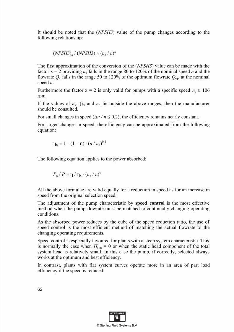
2.2.2.4 In the case of speed variation of a centrifugal pump, the pumpcharacteristic curve varies in accordance with the pump affinity laws. The followingrelationships apply for the flowrate and head:

Qx / Q = nx / n

H x / H = (nx / n)²

If the H (Q) curve is known for one speed ofrotation n then it can be converted for anotherspeed nx . The intersection of the new H x (Qx)

curve with the system curve gives the newduty point.

Fig. 2.15 Change of flowrate due to change of speed of rotation.




62

It should be noted that the ( NPSH3) value of the pump changes according to thefollowing relationship:

( NPSH3)x / ( NPSH3) (nx / n)x

The first approximation of the conversion of the ( NPSH3) value can be made with thefactor x = 2 providing nx falls in the range 80 to 120% of the nominal speed n and theflowrate Qx falls in the range 50 to 120% of the optimum flowrate Qopt at the nominalspeed n.

Furthermore the factor x = 2 is only valid for pumps with a specific speed ns 106rpm.

If the values of nx, Qx and nq lie outside the above ranges, then the manufacturershould be consulted.

For small changes in speed (n / n 0,2), the efficiency remains nearly constant.

For larger changes in speed, the efficiency can be approximated from the followingequation:

x 1 – (1 – ) · (n / nx)0,1

The following equation applies to the power absorbed:

P x / P / x · (nx / n)³

All the above formulae are valid equally for a reduction in speed as for an increase inspeed from the original selection speed.

The adjustment of the pump characteristic by speed control is the most effectivemethod when the pump flowrate must be matched to continually changing operatingconditions.

As the absorbed power reduces by the cube of the speed reduction ratio, the use ofspeed control is the most efficient method of matching the actual flowrate to the

changing operating requirements.

Speed control is especially favoured for plants with a steep system characteristic. Thisis normally the case when H stat = 0 or when the static head component of the totalsystem head is relatively small. In this case the pump, if correctly, selected alwaysworks at the optimum and best efficiency.

In contrast, plants with flat system curves operate more in an area of part loadefficiency if the speed is reduced.




63

In such cases it may be better to divide the total flowrate between a multiple ofequally sized pumps, or even different sizes, but without speed control. Anotheralternative is to operate a base load pump at constant speed and to satisfy the peakloads with speed controlled pumps.

Fig. 2.16 Characteristic of a single stage volute case pump with speed control

The figure also shows the interaction between the pump characteristic and flat andsteep system characteristics.




64

The principal pump drives with speed control are:

Three phase motor with frequency inverter

Pole-changing three phase motor

Three phase motor with mechanical, hydraulic or combination of mechanical andhydraulic speed control.

For further information on drives see section 9.6, “Speed control of electrical drive”.

For larger drive power, e.g. for boiler feed pumps in thermal power stations, steamturbines are often used above 8MW and these can generally be speed regulated.

Speed variation is normally employed when impeller reduction or other methods ofmatching the operating conditions are not considered viable for hydraulic oreconomic reasons.

This applies to both waste water pumps and pumps for handling solids, which have

specially designed impellers. If such a pump does not meet the required Q and H atdirect coupled motor speed, due to the hydraulic design, then the necessary speed toachieve the operating data with the pump in question is calculated. The pump is thendriven by belt drive or gearbox at the required increased or decreased speed.

Speed variation is also of advantage if an economic pump selection is not possiblewith a direct coupled motor.

Operating speeds up to 7000 rpm are common especially for multistage high pressure pumps, e.g. boiler feed pumps and also special pumps e.g. pitot tube pumps. Such pumps are normally gearbox driven. To achieve speed variation a hydraulic speedcontroller is added. For higher powers steam and gas turbines are also used.

With any change of pump speed, especially increased speed, the hydraulic speedlimitation with regard to the ( NPSH ) value and the mechanical speed limitation of the pump and drive must be considered.

In accordance with the formula, an increase in the ( NPSH3) value as the square of thespeed ratio must be calculated and consequently the available ( NPSH ) value of the plant ( NPSHA) could set a limit on the speed increase.

The mechanical speed limitation is dependent on the limiting values of the bearings,the lubrication, the shaft loading ( P /n value), the shaft seals (slip speed vg) and thematerial of the impeller.




65

Table 2.01 Maximum permissible tip speed of impeller dependent on materials.

Material example umax all in m/sGrey cast iron EN-JL1040 EN-GJL-250 40

Spheroidal graphite cast iron

Bronze and brass

EN-JS1030 EN-GJS-400-15

2.1050 G-CuSn 10

50

Stainless steels (normal) 1.4008 GX7CrNiMo12-1 95

Stainless steels (special) 1.4317 GX4CrNi13-4 110

Speed reduction generally gives no problems, but with multistage pumps with axial

thrust balance (relief devices) the minimum speed for the full effectiveness of thedevice must be observed.

2.2.2.5 Pre-rotation control utilises the effect of the pre-rotation of the liquidflowing into a centrifugal pump on the H (Q) characteristic. Positive pre-rotation (i.e. pre-rotation in direction of rotation of impeller) in any type of centrifugal pumpresults in reduction in the H (Q) characteristic compared to inflow without pre-rotation. Negative pre-rotation (i.e. pre-rotation in opposite direction to rotation ofimpeller) lifts the H (Q) characteristic. The pre-rotation for this type of control isinduced by adjusting the angle of incidence of a cascade of inlet guide vanes

upstream of the impeller.

The control range for the application of pre-rotation techniques depends principallyon the specific speed of the pump. Whilst in the case of radial flow pumps, theinfluence of pre-rotation is hardly noticeable, its influence increases with increasingspecific speed, i.e. in mixed flow pumps and axial flow pumps. For these pumps the point of optimum efficiency opt is generally achieved at rates of flow where optimuminflow conditions to the impeller exist. By modifying the inflow conditions, thisoperating point is changed, whilst at the same time the efficiency drops only slightly,so that control by pre-rotation can be considered a low loss method of control.

The use of a flap guide with variable geometry profile (flap diffuser), in place ofthe normal inlet guide vanes, holds the efficiency nearly constant over an even wider H (Q) range.

The most advantagous use of pre-rotation control is given by the position and shapeof the pre-rotation dependent H (Q) and (Q) curves, when only relatively smallchanges in flowrate are required for large changes in the system head.




66

Fig. 2.17 Characteristic field for a tubular casing pump with mixed flow impellerand pre-rotation.

The field shows the maximum limit for continuous operation. Above this limit the pump is likely to operate roughly.




68

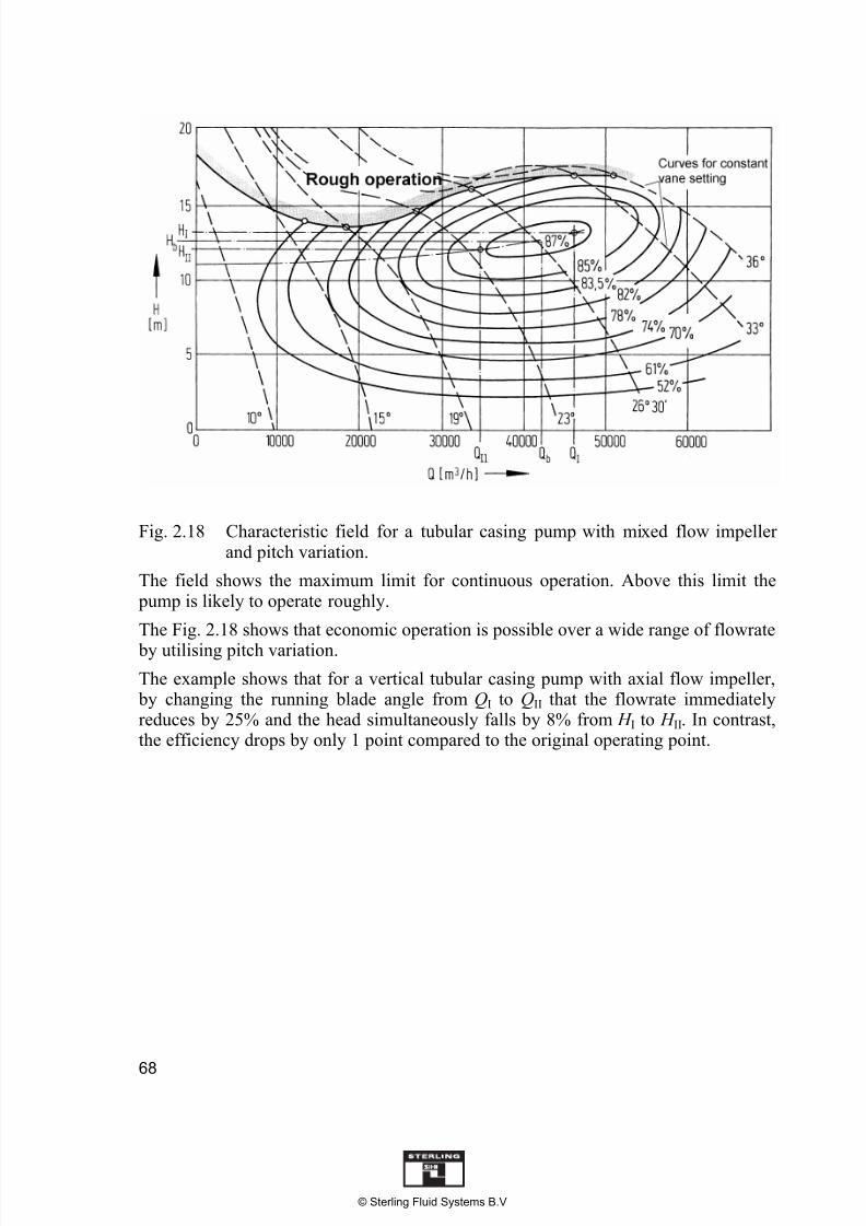
Fig. 2.18 Characteristic field for a tubular casing pump with mixed flow impellerand pitch variation.

The field shows the maximum limit for continuous operation. Above this limit the pump is likely to operate roughly.

The Fig. 2.18 shows that economic operation is possible over a wide range of flowrate

by utilising pitch variation.

The example shows that for a vertical tubular casing pump with axial flow impeller, by changing the running blade angle from QI to QII that the flowrate immediatelyreduces by 25% and the head simultaneously falls by 8% from H I to H II. In contrast,the efficiency drops by only 1 point compared to the original operating point.




69

2.3 Effect on the characteristics by installation of an orifice plate.

2.3.1 General

If the H (Q) characteristic is to be matched to a modified duty point in anapplication where an extremely steep characteristic curve is required to meet

control and installation considerations, it cannot normally be achieved bymodifying the pump hydraulics only, particularly in the case of mass produced

pumps. The only method is to install an orifice plate between the pump discharge branch and delivery pipeline. It should be noted that this constitutes pure throttlingin which the losses affect the characteristic curves of the pump directly.

The pressure loss due to an orifice platefollows a square relationship or parabolicform:

px = H x · · g = const. · Qx²

The new characteristic curve of thecentrifugal pump achieved by installing theorifice plate, differs from the normalcharacteristic at every point by the pressuredrop px.

As the pressure loss is proportional to the square of the flowrate Q , only two pointscan be specified and guaranteed for any one orifice plate. All additional pointseither have to lie on the calculated curve, or can only be achieved by using severalorifice plates which have to be changed for each set of points. Limits are thereforeset as to the choice of these points.

The shut off head of the desired H (Q) characteristic cannot exceed the value ofthe original characteristic curve (Fig. 2.21)

The slope of the desired H (Q) characteristic cannot be less steep than theoriginal characteristic curve (Fig. 2.22)

Fig. 2.19 Orifice plate design parameters Fig. 2.20 Influence of an orifice plateon the characteristic




70

When checking the H (Q) characteristic obtained by using an orifice plate, it should be noted that the measuring point should be no less than 6 x DN (DN = nominal bore of pipeline) downstream of the orifice plate, as the permanent pressure drop is present only after this distance (see also DIN EN ISO5167-1 Code of flowmeasurement).

2.3.2 Determining the diameter of the orifice plate

Depending on the location of the twoguaranteed points, there are in principle twocases to be distinguished in determining thediameter of the orifice plate:

Case I: The shut off head of the pump is notto be modified. In this case the diameter ofthe orifice plate and hence the pressure dropshould be determined so that the

characteristic curve achieves the 2nd

guarantee point.

The diameter d (Fig. 2.19) can be determined by means of the nomogram in table 13.19,following the example.

Fig. 2.23 Characteristic field for twooperating points

Case II: The required slope of the characteristic curve is expressed by twoarbitrary points on the characteristic curve H (Q) (Fig. 2.23), however thelimitations quoted in section 2.3.1 should be borne in mind.

Using the following values:

the following results are obtained for:

H 0 < 0: Configuration cannot be achieved, as H 0' > H 0 (Fig. 2.21)

H 0 = 0: H 0' = H 0, i.e. Case I

Fig. 2.21 Not achievable characteristic Fig. 2.22 Achievable characteristic

H I · QII² – H II · QI² with H I and H II in m

H 0 = —————————— in m

QII² – QI² and QI and QII in m³/h




71

H 0 > 0:

The desired characteristic curve can be achieved only by a reduceddiameter impeller (or impellers in the case of multistage pumps). After therequired impeller diameter has been calculated for the shut off head, H 0' =

H 0 – H0 and the corresponding H (Q) characteristic (see section 2.2.2.1 ),one proceeds as for case 1. It is immaterial for which of the two guarantee

points the diameter of the orifice plate is determined. It is recommendedhowever, that the calculation is made for both points as a check.

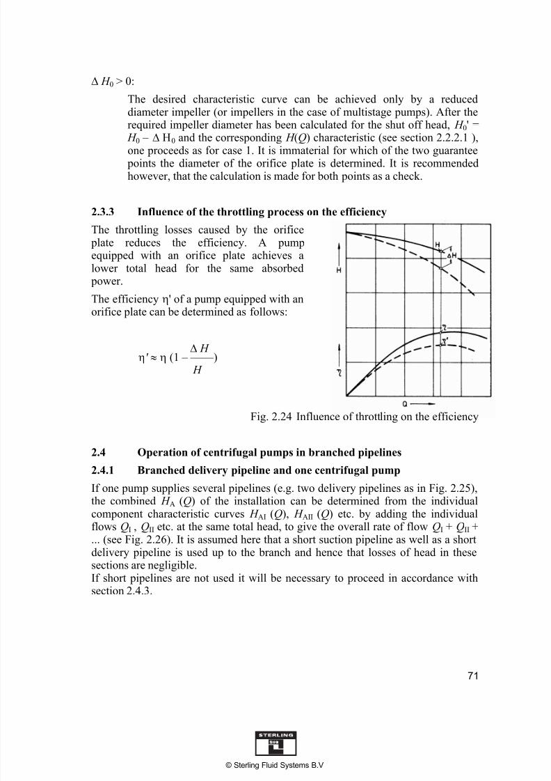
2.3.3 Influence of the throttling process on the efficiency

The throttling losses caused by the orifice plate reduces the efficiency. A pumpequipped with an orifice plate achieves a

lower total head for the same absorbed power.

The efficiency ' of a pump equipped with anorifice plate can be determined as follows:

Fig. 2.24 Influence of throttling on the efficiency

2.4 Operation of centrifugal pumps in branched pipelines

2.4.1 Branched delivery pipeline and one centrifugal pump

If one pump supplies several pipelines (e.g. two delivery pipelines as in Fig. 2.25),the combined H A (Q) of the installation can be determined from the individualcomponent characteristic curves H AI (Q), H AII (Q) etc. by adding the individualflows QI , QII etc. at the same total head, to give the overall rate of flow QI + QII +... (see Fig. 2.26). It is assumed here that a short suction pipeline as well as a shortdelivery pipeline is used up to the branch and hence that losses of head in thesesections are negligible.If short pipelines are not used it will be necessary to proceed in accordance withsection 2.4.3.

H ' (1 – ——)

H




72

Fig. 2.25

Pump with branched delivery

Fig. 2.26

Characteristic for the installation per Fig. 2.25

The duty point of the pump occurs at the intersection of the H (Q) characteristicwith the H A(Q) characteristic of the system. The horizontal line, (line of equal totalhead) though the duty point intersects the individual component curves H AI (Q),

H AII(Q) etc. at the flowrates of the respective branches of the pipeline. (Fig. 2.26).

If the static head of the branches is not identical H stat ( see example in Fig. 2.25), anon-return valve must be installed in each of the pipeline branches to prevent

backflow e.g. one container emptying in to the other when the pump has stopped.

2.4.2 Operation of centrifugal pumps in parallel into a common pipeline

If as shown in Fig. 2.27, two pumps with characteristic curves H I (Q) and H II (Q)supply a common pipeline having the system characteristic H A(Q) (assuming thatthe loss of head of the two pipelines up to the confluence is negligible), a common

H (Q) curve is constructed by adding the flows QI and QII of the individual pumps atthe same total head (Fig. 2.28).

At the intersection of the characteristic curves H (Q) and H A(Q) the total flow passing through the pipeline is given. The horizontal line (line of equal head)

through this point determines the duty points of the individual pumps on theirrespective characteristics and hence the component flows QI and QII. Note thatthese component flows are less than the rates of flow QI' and QII', which would beachieved by each of the pumps operating singly.

This feature is more noticeable with flatter pump characteristic curves and a steepersystem characteristic (Fig. 2.29).




73

It should be noted that in such cases,when operating in parallel, theindividual pumps operate in areas ofvery poor efficiency and no substantialincrease in flowrate can be achieved.

In the case of a very steep systemcharacteristic curve, the flow can beincreased more by operating the pumpsin series rather than in parallel.

Fig. 2.29 Characteristic for the plant as Fig 2.27 with a steep system curve andflat pump characteristic

Identical pumps with unstable H (Q) characteristics (see also section 2.1.3 ),

generally operate in parallel without trouble in systems with a “fixed” pipeline, bearing in mind that the total head of the 1st pump in the duty point (QI,II; H I,II) issmaller than the shut off head of the 2nd pump. The 2nd pump can only be startedunder this condition (Fig. 2.30).

If both pumps are used in a plant with a system characteristic, as shown with a broken line in this diagram, then this method cannot be used.

Fig. 2.27 System with two pumps

in parallel operation

Fig. 2.28 Characteristic for the plant as Fig

2.27 with a flat system curve andsteep pump characteristic




74

The operating parameters should bedrawn in all cases, but especially if

dissimilar pumps with unstable H (Q) characteristics are used. Onlythen can it be safely determinedwhether one of the pumps, or bothin the case of parallel operation, isworking in an area where flowoscillations or undesirable pressuresurges may occur (see section2.1.3).

Fig. 2.30

Characteristic for the plant as Fig 2.27 with an unstable H (Q) characteristics

2.4.3 Operation of centrifugal pumps in parallel with separate andcommon pipeline sections

In this case the flowrates of the individual pumps (in Fig. 2.31 two pumps are

shown) add up only at point A, the start of the common section of the pipeline. Thismeans that the total head values of the component flows have to be identical at this point.

Fig. 2.31 Operation of centrifugal pumps in parallel with separate and common pipeline sections




75

The total head at point A is obtained from the H I (Q) or H II (Q) characteristics of theindividual pumps by reducing them by the head H AI (Q) or H AII (Q) respectively, ofthe separate sections of the pipeline (Fig. 2.32 and 2.33).

These reduced H I red (Q) and H II red (Q)characteristics can be added to a

common H red (Q) “characteristic”, as insection 2.4.2, by adding the flowratesat the same total head. The intersectionof this “characteristic curve” with thecharacteristic curve H AIII (Q) of thesystem representing the commonsection of the pipeline establishes theflowrate QI+II.

Fig. 2.34 Characteristic for the common section of pipeline

The component flows Qi and Qii are obtained at the intersection of the horizontalline with the individual reduced characteristic curves. At these flows Qi and Qii

respectively of the individual pump, the H , P , and ( NPSHR) can be read off.

Fig. 2.32 Reduced characteristic curve of pump 1 at point A

Fig.2.33 Reduced characteristic curveof pump 2 at point A




76

2.4.4 Operating centrifugal pumps in series into a common pipeline

When operating centrifugal pumps in series in a system with a common pipeline, thetotal head values of the individual pumps add up at the same flowrate to give the totalhead of the series combination.

In the case of unequal pumps, it is expedient to arrange the pump with the lowest( NPSHR) as the first in the series.

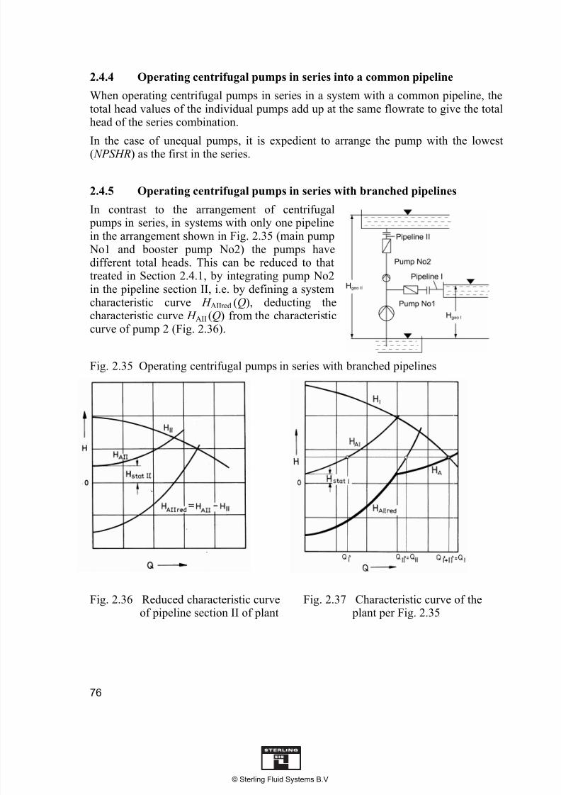
2.4.5 Operating centrifugal pumps in series with branched pipelines

In contrast to the arrangement of centrifugal pumps in series, in systems with only one pipelinein the arrangement shown in Fig. 2.35 (main pump No1 and booster pump No2) the pumps havedifferent total heads. This can be reduced to that

treated in Section 2.4.1, by integrating pump No2in the pipeline section II, i.e. by defining a systemcharacteristic curve H AIIred (Q), deducting thecharacteristic curve H AII (Q) from the characteristiccurve of pump 2 (Fig. 2.36).

Fig. 2.35 Operating centrifugal pumps in series with branched pipelines

Fig. 2.36 Reduced characteristic curveof pipeline section II of plant

Fig. 2.37 Characteristic curve of the plant per Fig. 2.35




77

This characteristic curve H AII red (Q) is added to the characteristic curve H AI (Q) of the pipeline section I to obtain a common system characteristic H A (Q) in accordance withsection 2.4.1. Its intersection with the H (Q) characteristic of pump No1 gives the duty point of pump No1 (Fig. 2.37). The horizontal line through this duty point intersectsthe characteristic curves H AI and H AII red at the component flows QI’ and QII’. The

component flow QII’ is equal to the component flow QII of Pump No2.

2.5 Start up and run down of centrifugal pumps

Occasionally the conditions during start up and run down of centrifugal pumps may be decisive in the operation of a centrifugal pump installation. In such cases it isimportant to know the starting torque and start up and run down times of the pump.

2.5.1 The starting torque M P is the torque required by the pump during startingto maintain the running speed reached at each point in time.

The value increases from zero when stepped up to the nominal torque. In contrast theabsorbed torque transmitted via the coupling M m is mainly dependent on the driver.Until the nominal torque M N is reached, the transmitted torque exceeds the startingtorque. The difference between these two torque values is the acceleration torque M b,which increases the speed of the entire rotating mass in the pumpset.

M b = M m – M P

P M P = 9549 · — in N m with P in kW, n =rpm

n

Fig. 2.38 Run up of a centrifugal pump in H (Q) diagram

Fig. 2.39 Run up of a centrifugal pump in /(n) diagram




78

Because in a set of H (Q) curves (Fig. 2.38), a specific rotational speed and a specifictorque is associated with every possible duty point, the shape of the starting torquecurve is determined by the line along which the operating point of the pump movesfrom zero to the operating point “B” at nominal speed. Basically four different casescan be distinguished (see Fig. 2.38 and 2.39 for an example of a low specific speed

radial flow pump in which the absorbed power P rises with increasing flowrate Q).

1. Starting against a closed valve which is opened after the nominal speedhas been reached

Line 0 - A – B (Fig 2.38)

For the section 0 - A the hydraulic torque of the pump increases as the square of therotational speed. This torque has to be increased to overcome friction in the bearingand shaft seals, which accounts for a relatively high percentage of the starting torqueat low rotational speeds. At n=0 the static friction, also known as break-out torque, is

particularly high.

Static friction normally amounts to approximately 5 to 10% of the nominal torque. In pumps with overhung impeller arrangements and high inlet pressure its value mayreach the order of magnitude of the nominal torque.

For the section A-B the starting torque - now at constant rotational speed - increasesor decreases as a function of the shape of the pump power input curve. Side channel pumps and axial flow pumps, where at Q=0 the power input and hence the startingtorque is higher than at the duty point, should not be started in this way.

2. Starting with an open valve with a purely static system head acting onthe non-return valve

Line 0 - C – B (Fig 2.38)

In this instance the shape of the starting torque curve is identical with the previouscase of starting against a closed valve, up to the point C, as only at this point can thenon-return valve be opened by the pump delivery pressure and flow commence. Thefurther path of the torque curve is established by constructing intermediatecharacteristic curves for H (Q) for the section C - B at different rotational speeds (seesection 2.2.2.4) and by calculating the torque from the power input. In practice it isoften sufficient to make an assumption for the course of the torque to be linear between “C” and “B”, whilst the rotational speed for point “C” is calculated from:

nC = n N · ( H stat / H 0)0,5 with n in rpm, H in m




79

3. Starting with an open valve against a purely dynamic system head

Line 0 – B (Fig 2.38)

This only occurs if the pipeline is very short. The starting torque M P increases, apartfrom the torque due to static friction, as the square of the rotational speed from zero to

the nominal torque.

If on the other hand the pipeline is very long, the time required to accelerate the massof water is considerably longer than the starting time for the pump. The mass of waterat rest, acts in this case like a closed valve and the starting torque takes a similarcourse to case 1.

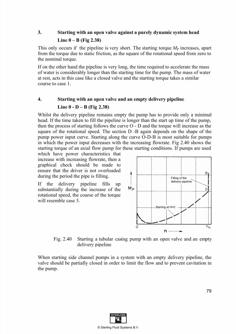
4. Starting with an open valve and an empty delivery pipeline

Line 0 - D – B (Fig 2.38)

Whilst the delivery pipeline remains empty the pump has to provide only a minimalhead. If the time taken to fill the pipeline is longer than the start up time of the pump,then the process of starting follows the curve O - D and the torque will increase as thesquare of the rotational speed. The section D -B again depends on the shape of the pump power input curve. Starting along the curve O-D-B is most suitable for pumpsin which the power input decreases with the increasing flowrate. Fig 2.40 shows thestarting torque of an axial flow pump for these starting conditions. If pumps are usedwhich have power characteristics thatincrease with increasing flowrate, then agraphical check should be made toensure that the driver is not overloaded

during the period the pipe is filling.

If the delivery pipeline fills upsubstantially during the increase of therotational speed, the course of the torquewill resemble case 3.

Fig. 2.40 Starting a tubular casing pump with an open valve and an emptydelivery pipeline

When starting side channel pumps in a system with an empty delivery pipeline, thevalve should be partially closed in order to limit the flow and to prevent cavitation inthe pump.




80

2.5.2 The start up time of a centrifugal pump results from the difference between the input torque M m (torque transmitted via the coupling) and the startingtorque M P, i.e. from the excess torque M b, which is available for acceleration of theentire rotating mass of the pumpset, from speed n = 0 until the nominal rotationalspeed n N has been reached.

M b = M m – M P

Fig. 2.41 shows how the inputtorque M m and the starting torqueof the pump M P and therefore theacceleration torque M b aredependent on the rotational speed.

Fig. 2.41 M (n) chart for DOLstarting of electric motor and startup of pump as in case 3(see 2.5.1)

As these interdependent functionsare generally not available in analytical form it is usual to derive a mean acceleratingtorque from the mean input and starting torque.

M b mi = M m mi – M P mi

Fig. 2.42. shows a sufficientlyaccurate method of establishing themean accelerating torque. It can becalculated for example by countingthe squares on graph paper for theinput and starting torque curves.

The time t A to reach the nominal

speed n N is calculated from theequation:

Fig. 2.42 Establishing mean accelerating torque

n N · J gr t A = —— · ———— in secs

30 M b mi




81

In this equation:

n N = Nominal speed rpm

J gr = Moment of inertia of entire rotating mass in kg m²

M b mi

= Mean accelerating torque in N m

The total moment of inertia J gr comprises the moments of inertia of the motor, pump,coupling and where applicable gearbox or belt drive system. It is always referred tothe speed of the motor.

If the speed of the motor and pump are different, the moment of inertia J P (Sum of themoments of inertia of all components rotating at the pump speed nP) can beinterpolated to the motor speed with the following equation;

As a result of the favourable torque ratio ( M m : M P) of centrifugal pumps and therelatively low moment of inertia, the starting time is well within the limits of that ofelectric motors and so present no problems.

2.5.3 The run-down time of a centrifugal pump is found in the same way as thestart up time if the starting torque M P is known as a function of the rotational speed n .

Since during the run down of the pump, as a result of switching off or failure of thedriver, the driving torque M m moves toward zero and the starting torque of the pump becomes a retarding torque M v.

The run down time, i.e. the time for the pump to come to a stand still after switching

off the driver, is calculated from the following equation:

where n N = Rotational speed rpm

J gr = Total moment of inertia of unit in kg m²

M v mi = Mean retarding torque in N m

In general the moment of inertia J gr of the rotating components is small so thatcentrifugal pumps run down quickly. In very long pipeline systems this may lead,under certain conditions, to pressure surges which exceed the pressure limitations ofcomponents in the system. This could lead, in extreme cases, to failure of the pipeline, fittings or instruments, see also section 4.7. Increasing the moment of inertia J gr by the addition of a flywheel can increase the run down time, but whether possible pressure surges are prevented must be checked, in each case.

nP ² J P’ = J P · ——

nMot

n N · J gr t aus = —— · ———— in secs

30 M v mi




82

2.6 Minimum and Maximum Flowrate

2.6.1 Minimum flowrate due to internal power losses

The power loss P int causes a rise in temperature of the pumped liquid. If the normallysmall heat dissipation through radiation and conduction is neglected, then the heat

generated equivalent to the power loss must be removed by the flow of liquid:

P int = q · c · T = · Q · c · T

or in numerical terms:

P int = 0,278 · · Q · c · T in kW

with in kg/dm³, Q in m³/h, c = specific heat in kJ/kg K

c - Values for various liquids see tables 13.16 and 13.17

The internal power loss P int is calculated from the power absorbed by the pump P after deducting the external mechanical power loss P m and the hydraulic power P u:

The temperature increase is given by:

or in numerical terms:

Fig. 2.43 Power loss P int dependent on Q

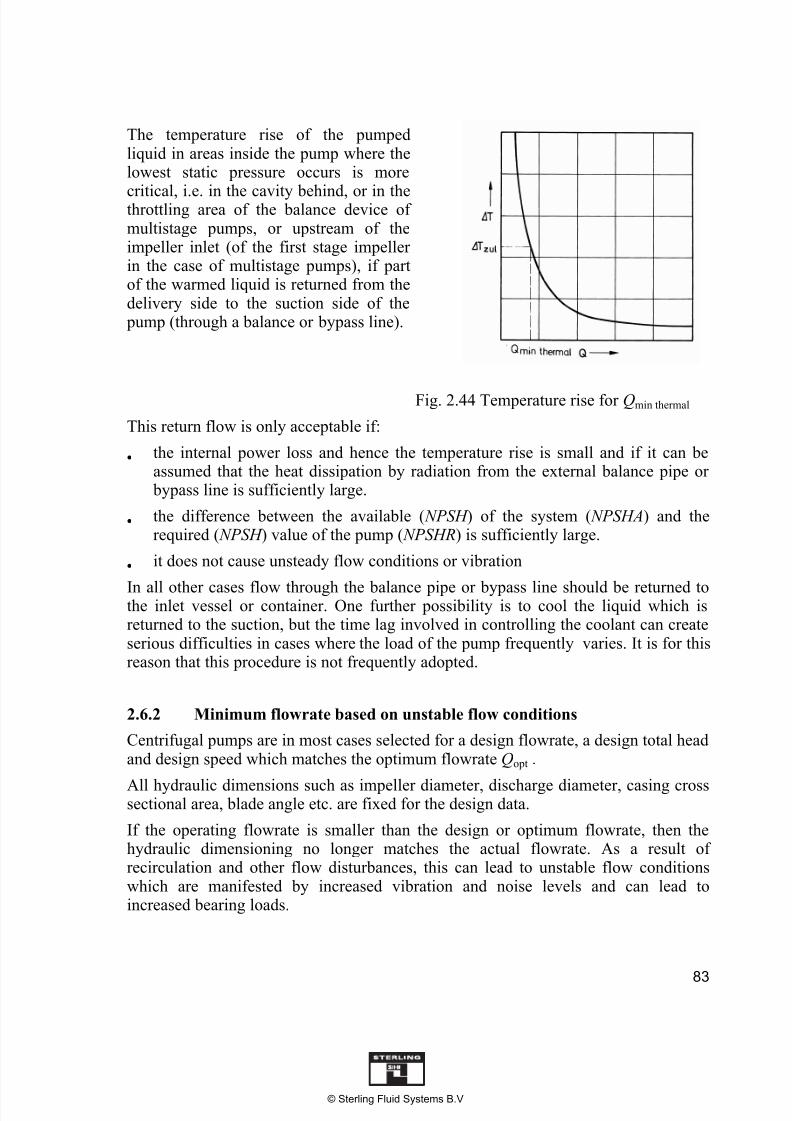
Fig. 2.43 shows schematically these conditions for a low specific speed centrifugal

pump.Fig. 2.44 shows the curve of the temperature rise T as a function of the flowrate Q.Theoretically, at Q = 0 the temperature rise is infinite. If the maximum permissibletemperature rise is T zul the flowrate must not drop below the minimum value, alsoknown as the thermal flowrate Qmin thermal. The curve T/ (Q) has to be established point by point and Qmin thermal has to be read off at the pre-determined value T zul .

The maximum temperature occurs in the outlet branch of the pump where, due to the prevailing pressure, no danger arises from the vaporisation of the pumped liquid.

m

P int = P – P m – P u = · g · Q · H · (—— – 1)

P – P Jm – P u g · H m T = —————— = ——— (—— – 1)

· Q · c c

H mT = 0,01 · — · (—— – 1) in K

c

with H in m, c in kJ/kg K




83

The temperature rise of the pumpedliquid in areas inside the pump where thelowest static pressure occurs is more

critical, i.e. in the cavity behind, or in thethrottling area of the balance device ofmultistage pumps, or upstream of theimpeller inlet (of the first stage impellerin the case of multistage pumps), if partof the warmed liquid is returned from thedelivery side to the suction side of the pump (through a balance or bypass line).

Fig. 2.44 Temperature rise for Qmin thermal

This return flow is only acceptable if:

the internal power loss and hence the temperature rise is small and if it can beassumed that the heat dissipation by radiation from the external balance pipe or bypass line is sufficiently large.

the difference between the available ( NPSH ) of the system ( NPSHA) and therequired ( NPSH ) value of the pump ( NPSHR) is sufficiently large.

it does not cause unsteady flow conditions or vibration

In all other cases flow through the balance pipe or bypass line should be returned tothe inlet vessel or container. One further possibility is to cool the liquid which isreturned to the suction, but the time lag involved in controlling the coolant can createserious difficulties in cases where the load of the pump frequently varies. It is for thisreason that this procedure is not frequently adopted.

2.6.2 Minimum flowrate based on unstable flow conditions

Centrifugal pumps are in most cases selected for a design flowrate, a design total headand design speed which matches the optimum flowrate Qopt .

All hydraulic dimensions such as impeller diameter, discharge diameter, casing crosssectional area, blade angle etc. are fixed for the design data.

If the operating flowrate is smaller than the design or optimum flowrate, then thehydraulic dimensioning no longer matches the actual flowrate. As a result ofrecirculation and other flow disturbances, this can lead to unstable flow conditionswhich are manifested by increased vibration and noise levels and can lead toincreased bearing loads.




84

In continuous operation, to prevent pump operating problems and damage, operation below the manufacturer’s minimum permissible flowrate Qmin stable, which is known asthe “minimum stable flowrate” should be avoided.

2.6.3 Maximum flowrate

If the operating flowrate is higher than the selection and/or optimum flowrate, thenthe points in the preceding section 2.6.2 are relevant, i.e. these operating conditionscan also cause unstable flow conditions.

In continuous operation, to prevent pump operating problems and damage, operationabove the manufacturer’s maximum permissible flowrate Qmax stable which is known asthe “maximum stable flowrate” should be avoided.

The maximum permissible flowrate can also be limited by the ( NPSH ) value of thesystem ( NPSHA), if the ( NPSH ) value of the pump ( NPSHR), increasing with theflowrate, becomes larger than the ( NPSHA). These operating conditions are notsuitable for continuous operation. See also section 1.5.4, and 2.1.3.

2.6.4 Recommended limits for minimum and maximum flowrate incontinuous operation

The following table gives the recommended limits of Qmin stable and Qmax stable, forcontinuous operation, for different types of pump, dependent on the specific speed ns,on the assumption that the ( NPSH ) value permits (see section 1.5.4).

When establishing the limits for side channel pumps, axial flow pumps andcentrifugal pumps with unstable characteristics, the sections 2.1.1, 2.1.3, and 2.4.2,should be considered.

Pump type Side channel pumps

Centrifugal pumps

Mixed flow pumps

Axial flow pumps

ns 4 ... 12 8 ... 45 40 ...160 100 ... 300

Qmin stable/Qopt 0,10 ... 0,64 0,10 ... 0,40 0,60 ... 0,65 0,75

Qmax stable/Qopt 1,10 ... 1,40 1,50 1,35 1,10

Table 2.02 Recommended limits for continuous operation

The limits for multistage ring section pumps with thrust balance are set much moreclosely and therefore it is important that the data provided by the manufacturer isobserved.

This also applies to canned motor pumps and pumps with a magnetic coupling.




85

2.6.5 Protection of centrifugal pumps

If the operation of the plant means that the pump may be working against a closedshut off or control valve or similar, it is necessary to protect the pump from operating below the minimum flow. This applies generally for all types of pump, but especially

for multistage high pressure pumps with common relief devices against axial thrust.This is important, as with this type of pump, falling below the minimum flow leads toevaporation of the pumped liquid in the spaces in the relief device, which can causeimmediate failure of the pump with considerable damage.

There are several possible methods of protection

Continuous return of the minimum flowrate through a by-pass line with a fixedorifice plate. With this method, the minimum flow must be added to the nominalflow for the pump selection.

Return of the minimum flowrate through a by-pass line with a fixed orifice plateand an open/shut valve. The valve is opened when the flow in the main pipelinefalls below the minimum flowrate.

Regulation of the minimum flowrate through an automatic by-pass valve, e.g. afree flow non-return valve. The spring operated non-return valve is flowdependent. The setting of the valve, controls the by-pass flow. It is set so that the by-pass line opens as soon as the flow in the main pipeline falls below theminimum flowrate. When the non-return valve is closed the by-pass is fully open.This method is used principally for boiler feed and condensate pumps.

Regulation of the minimum flowrate through a modulating valve. The modulatingvalve can be controlled by the flow in the main pipeline, from pressure or

temperature difference, or from the absorbed power of the drive motor, howevercontrol by the flowrate is the most reliable method.

Operational Performance of Centrifugal Pumps

Documents

Transcript of Operational Performance of Centrifugal Pumps