Business Processes - Operational Solutions for SAP Implementation

Operational
Implementation
and Cost
Analysis of a
LiDAR
inventory in
Boreal Ontario
Murray Woods
Southern Science & Information
OMNR – North Bay

FPInnovations: CWFC, Forest Ops.,
Wood Prod., Pulp&Paper
CFS: Luther, Leckie, Gougeon, Wulder, Beaudoin
Universities: UBC, Queen’s, Nipissing, Sherbrooke,
UQAM, Laval, Sir Wilfred Grenfell
Provinces: BCMoFR, ASRD, OMNR, MRNF-QC,
NLDNR, NBDNR
Industry: West Fraser, Tembec, Foothills G&Y,
Corner Brook P&P, J.D. Irving
Funding partners: GEOIDE, OCE, FQRNT, ACOA,
AIFI, NSERC
Regional Delivery
through Partnerships Partnerships
Canadian Wood Fibre Centre (CWFC) National Program
… inventory systems that support Value Chain Optimization by allowing us to
send the right wood to the right markets, at the right time !

Advanced
Forest
Resource
Inventory
Technologies

Kevin Lim Lim Geomatics
Image source: http://www.icejerseys.com/images/rbk_edge_replica_jerseys/TorontoMapleLeafsReebokPremierReplicaAltJersey_big.jpg
Doug Pitt
Paul Treitz
Margaret Penner Forest Analysis Ltd.
Dave Nesbitt
Jeff Dech Don Leckie François
Gougeon
ITC Line
Dave Etheridge
TEAM AFRIT
LiDAR 101
LiDAR Derived Inventory Primer
Current LiDAR Inventory Success Stories
Operational Decision Support Tools – AFRIDS
Operational Economics
Enhancements to Next Generation Inventories
Implementation and Cost Analysis of a LiDAR inventory
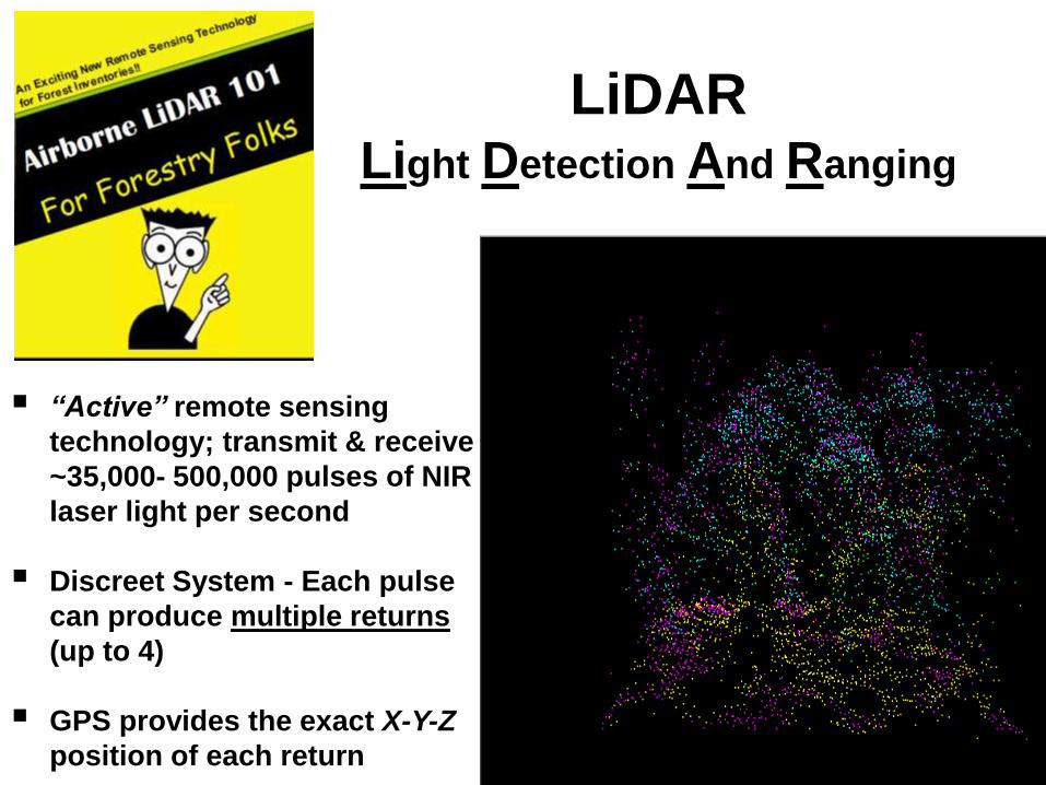
“Active” remote sensing
technology; transmit & receive
~35,000- 500,000 pulses of NIR
laser light per second
Discreet System - Each pulse
can produce multiple returns
(up to 4)
GPS provides the exact X-Y-Z
position of each return
LiDAR Light Detection And Ranging
Used with permission of Doug Pitt

Prince Edward County, Ontario Ground Hits -> DTM
LiDAR Technology
Historical Reason for Acquiring LiDAR Data
Lidar
5m OBM
20m

Prince Edward County, Ontario Ground Hits -> DTM
Vegetation Hits Only
LiDAR Technology

• High Resolution DTM
• Hazard mapping
• Floodplain/risk mapping
• Landform Classification-ELC
• Agricultural Land mapping
• Geological Mapping
• Open pit mining
• Coastal/Shoreline Mapping
• Predictive Hydrology
• Urban Modeling
• Woodlot Extraction
• Transmission Line corridors Forest Engineering
• Corridor/Right-of-way Mapping
• Wetlands/Riparian areas
• Habitat modeling
• Forest Inventory
www.botany.hawaii.edu/GISlab.htm
www. Saminc.biz
Airborne-LiDAR Informing Better Decisions
Ambercore.com

Field Sampling
• Cruising generally not
occurring in Boreal
forests
• Very “light” 1%-2%
• Expensive
• Only provides
information on sampled
sites – extrapolated
• Need to do for the next
stand…and the next…
Traditional Operational Cruising

Field Sampling vs. 100% Enumeration
LiDAR Derived Inventory
• 100% enumeration of the
landbase with LiDAR
measurements of vertical
structure
• permits the use of
regression estimators to
scale PU estimates to
groups of PUs, Stand,
Block or Forest

• LiDAR offers more than a DTM
• Additional forest inventory information contained in point cloud data
• Focus of AFRIT is “Area” based modeling NOT “Individual Tree”
• Prediction Unit = 20m X 20m (400m2)
LiDAR Derived Forest Inventory

LiDAR Derived Inventory – Pairing with Ground Data
Field Plot Measurement
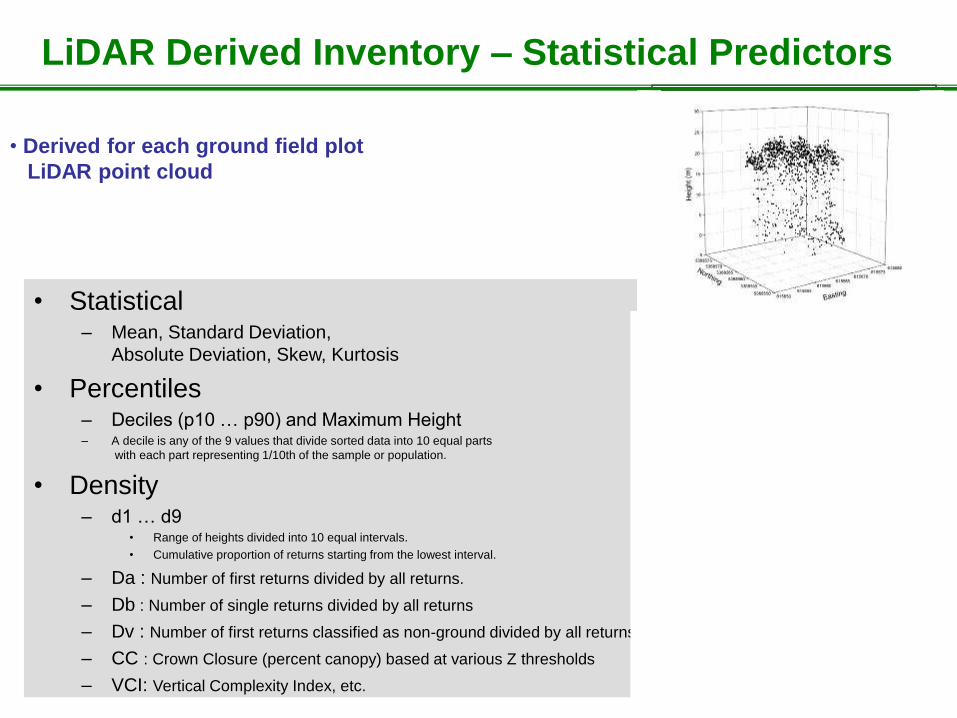
• Derived for each ground field plot
LiDAR point cloud
• Derived for each 400m2 (20m x 20m)
prediction unit of the landscape
20m
20m
• Statistical – Mean, Standard Deviation,
Absolute Deviation, Skew, Kurtosis
• Percentiles – Deciles (p10 … p90) and Maximum Height – A decile is any of the 9 values that divide sorted data into 10 equal parts
with each part representing 1/10th of the sample or population.
• Density – d1 … d9
• Range of heights divided into 10 equal intervals.
• Cumulative proportion of returns starting from the lowest interval.
– Da : Number of first returns divided by all returns.
– Db : Number of single returns divided by all returns
– Dv : Number of first returns classified as non-ground divided by all returns.
– CC : Crown Closure (percent canopy) based at various Z thresholds
– VCI: Vertical Complexity Index, etc.
Heig
ht
(m)
Heig
ht
(m)
%
m
LiDAR Derived Inventory – Statistical Predictors

Boreal Forest MU
• Romeo Malette Forest
~630k ha
• Hearst Forest
~ 1.3 M ha
Study Sites

• Height (AVG, Top) • QMDBH • Volume (GTV, GMV) • Basal area • Biomass • Density*
* Derived from DBHq & BA
LiDAR predictive Models for:
• Sawlog Volume • Close Utilization
Volume • Dom/Codom Ht • Mean Tree GMV • Size Class Distributions
Pre
dic
ted
Observed
LiDAR Derived Inventory
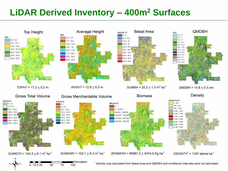
LiDAR Derived Inventory – 400m2 Surfaces

LiDAR
Information can
add more value
to our rich image
and inventory
interpretation
LiDAR Derived Inventory – 400m2 Surfaces
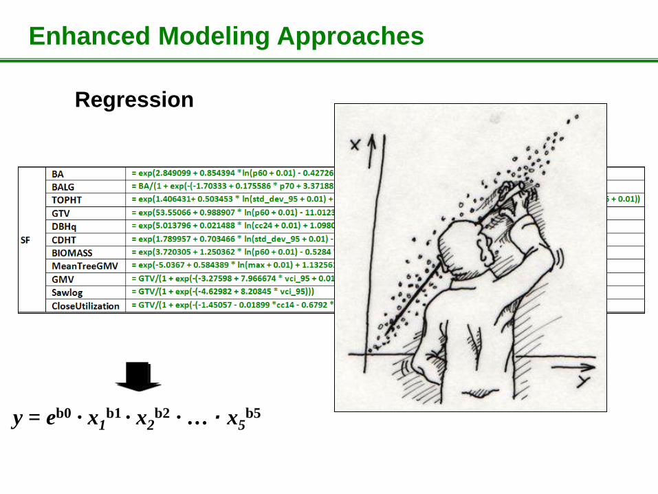
Enhanced Modeling Approaches
Regression
y = bo+ b1 x1+ b2 x2
y1 = bo+ b1 x1+ b2 x2
y2 = bo+ b1 x1+ b2 x3
yp = bo+ b1 x2+ b2 x3
y = eb0 · x1b1 · x2
b2 · … · x5b5

Enhanced Modeling Approaches
Regression RandomForest
y = bo+ b1 x1+ b2 x2
y1 = bo+ b1 x1+ b2 x2
y2 = bo+ b1 x1+ b2 x3
yp = bo+ b1 x2+ b2 x3
y = eb0 · x1b1 · x2
b2 · … · x5b5
Option for hundreds to thousands of trees

SUR vs. RandomForest - Predicted vs. Observed
SUR Regression Model RandomForest

LiDAR vs. RandomForest Models – CV (% of mean) by Forest Type
LiDAR Derived Inventory
Dom/Codom HT CV Comparison by Model Type
0% 5% 10% 15% 20% 25%
SB
SF
SP
PJ
IH
LC
MWC
MWH
Fo
res
t T
yp
e
Coefficient of Variation
Merch BA CV Comparison by Model Type
0% 5% 10% 15% 20% 25%
SB
SF
SP
PJ
IH
LC
MWC
MWH
Fo
res
t T
yp
e
Coefficient of Variation
GMV CV Comparison by Model Type
0% 5% 10% 15% 20% 25%
SB
SF
SP
PJ
IH
LC
MWC
MWH
Fo
res
t T
yp
e
Coefficient of Variation
DBHq CV Comparison by Model Type
0% 5% 10% 15% 20% 25%
SB
SF
SP
PJ
IH
LC
MWC
MWH
Fo
res
t T
yp
e
Coefficient of Variation
SUR RandomForest-Regression
Forest
Type N
SB 104
SF 46
SP 54
PJ 67
IH 67
LC 23
MWC 38
MWH 43

LiDAR Derived Inventory
SUR
LiDAR vs. RandomForest Models – CV (% of mean) by Forest Type
Dom/Codom HT CV Comparison by Model Type
0% 5% 10% 15% 20% 25%
SB
SF
SP
PJ
IH
LC
MWC
MWH
Fo
res
t T
yp
e
Coefficient of Variation
Merch BA CV Comparison by Model Type
0% 5% 10% 15% 20% 25%
SB
SF
SP
PJ
IH
LC
MWC
MWH
Fo
res
t T
yp
e
Coefficient of Variation
GMV CV Comparison by Model Type
0% 5% 10% 15% 20% 25%
SB
SF
SP
PJ
IH
LC
MWC
MWH
Fo
res
t T
yp
e
Coefficient of Variation
DBHq CV Comparison by Model Type
0% 5% 10% 15% 20% 25%
SB
SF
SP
PJ
IH
LC
MWC
MWH
Fo
res
t T
yp
e
Coefficient of Variation
RandomForest-Regression
DBHq RMSE (+/-) Comparison by Model Type
0.0 0.5 1.0 1.5 2.0 2.5 3.0 3.5 4.0 4.5 5.0
SB
SF
SP
PJ
IH
LC
MWC
MWH
Fo
res
t T
yp
e
+/- cm
SURRfreg

RandomForest LiDAR derived Inventory Surfaces
Advantages of RandomForest
• doesn't rely on an existing
polygon inventory
• no separate forest-type
models to statistically build
• very quick to implement
• custom application of LiDAR
predictions for each 20m x 20m
Disadvantages of RandomForest
• black box – “loss of control”
• Critical that extremes of forest
conditions are sampled as input
LiDAR Predicted GMV Raster

Value Added – RandomForest 1st-cut Stand Polygons
LiDAR Predicted GMV Raster

LiDAR Derived Inventory – 400m2 Surfaces
Developed with Polygon Forest-Type Knowledge
Developed solely from LiDAR input
(& eFRI polygons added for comparison to SUR)
Pockets of species within a typed stand

0
0.05
0.1
0.15
0.2
0.25
0.3
0.35
0.4
10 12 14 16 18 20 22 24 26 28 30 32 34 36 38 40
Diameter class (cm)
Re
lati
ve
fre
qu
en
cy
0
pred3
+
0
0.05
0.1
0.15
0.2
0.25
0.3
10 12 14 16 18 20 22 24 26 28 30 32 34 36 38 40
Diameter class (cm)
Re
lati
ve
fre
qu
en
cy
0.2
pred3
+
0
0.05
0.1
0.15
0.2
0.25
10 12 14 16 18 20 22 24 26 28 30 32 34 36 38 40
Diameter class (cm)
Re
lati
ve
fre
qu
en
cy
0.4
pred3
+
0
0.05
0.1
0.15
0.2
0.25
10 12 14 16 18 20 22 24 26 28 30 32 34 36 38 40
Diameter class (cm)
Re
lati
ve
fre
qu
en
cy
0.3
pred3
+
0
0.05
0.1
0.15
0.2
0.25
10 12 14 16 18 20 22 24 26 28 30 32 34 36 38 40
Diameter class (cm)
Re
lati
ve
fre
qu
en
cy
0.5
pred3
+
0
0.05
0.1
0.15
0.2
0.25
10 12 14 16 18 20 22 24 26 28 30 32 34 36 38 40
Diameter class (cm)
Re
lati
ve
fre
qu
en
cy
0.6
pred3
+
Black Spruce Validation Data
– Aggregated by VCI class
LiDAR Derived Inventory – Size-Class Distributions
Density and Volume by 2cm Diameter Classes

Mixedwood Validation Data
– Aggregated by VCI class
LiDAR Derived Inventory – Size-Class Distributions
Density and Volume by 2cm Diameter Classes
0
0.05
0.1
0.15
0.2
0.25
10 12 14 16 18 20 22 24 26 28 30 32 34 36 38 40
Diameter class (cm)
Re
lati
ve f
req
ue
ncy
0.6
pred3
0
0.05
0.1
0.15
0.2
0.25
10 12 14 16 18 20 22 24 26 28 30 32 34 36 38 40
Diameter class (cm)
Re
lati
ve f
req
ue
ncy
0.3
pred3
0
0.05
0.1
0.15
0.2
0.25
10 12 14 16 18 20 22 24 26 28 30 32 34 36 38 40
Diameter class (cm)
Re
lati
ve f
req
ue
ncy
0.5
pred3
+
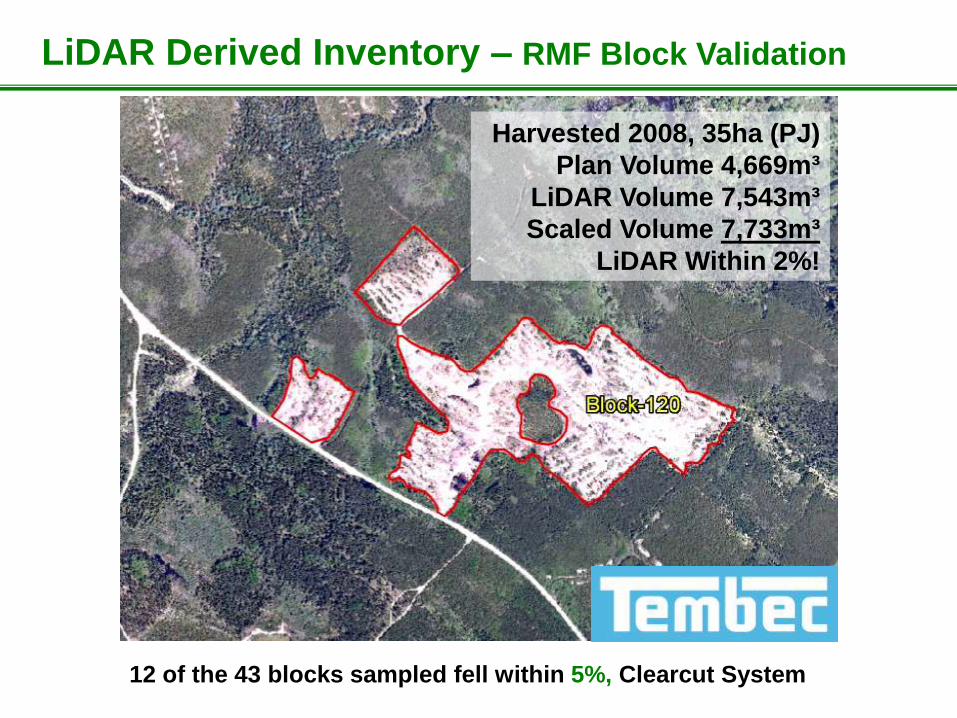
Harvested 2008, 35ha (PJ)
Plan Volume 4,669m³
LiDAR Volume 7,543m³
Scaled Volume 7,733m³
LiDAR Within 2%!
12 of the 43 blocks sampled fell within 5%, Clearcut System
LiDAR Derived Inventory – RMF Block Validation
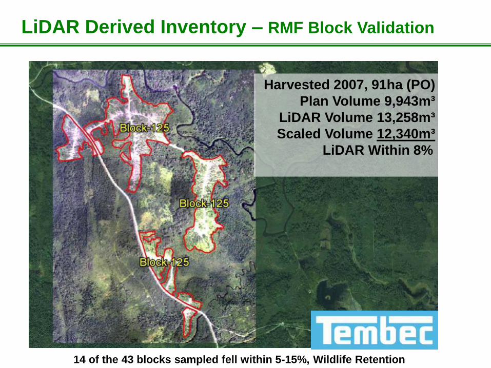
Harvested 2007, 91ha (PO)
Plan Volume 9,943m³
LiDAR Volume 13,258m³
Scaled Volume 12,340m³
LiDAR Within 8%
14 of the 43 blocks sampled fell within 5-15%, Wildlife Retention
LiDAR Derived Inventory – RMF Block Validation

Harvested 2009, 197ha (SB/LA)
Plan Volume 24,152m³
LiDAR Volume 16,606m³
Scaled Volume 13,238m³
LiDAR Within 25%
LiDAR Derived Inventory – RMF Block Validation
Inventory issues
- Sp Comp
- Age
- resultant Site Class
- resultant Yield Curve
Residual Sb

AFRIDS Advanced Forest Resource Inventory Decision Support System

AFRIDS Advanced Forest Resource Inventory Decision Support System

Forest Unit: SB1
Area: 45 ha
AFRIDS Advanced Forest Resource Inventory Decision Support System

AFRIDS Advanced Forest Resource Inventory Decision Support System


• Are LiDAR-enhanced
inventories leading to
better forest management
decisions?
• What are the cost savings
associated with enhanced
decision making?
Objectives

LiDAR provides better volume prediction (statistically tested)
– Yield Curve: 14.5%
– LIDAR: 5.4 %
Yield Curve BW SP PJ PO
208 12% 10% 0% -22%
214
216 -2% 33% 3% -34%
220 14% -15% 0% 1%
244 -9% 34% -12% -14%
245 -2% 9% -1% -6%
246 -2% 20% -1% -17%
251 6% 33% 6% -45%
252 9% 55% 1% -66%
254 -1% 4% 10% -12%
256 1% -6% 5%
257 7% -17% 9%
259 1% 0% -1%
275
LIDAR BW SP PJ PO
208 2% -6% 0% 3%
214
216 -16% 6% 1% 8%
220 0% -11% 4% 7%
244 -10% 2% 2% 5%
245 0% 5% 1% -6%
246 0% 5% 1% -6%
251 1% 11% 5% -17%
252 4% 23% 2% -29%
254 1% -4% 0% 4%
256 2% -1% -1%
257 2% -5% 3%
259 -3% -2% 5%
275
10 % & under greater than 10 %
Difference from harvested volume (scaled)
Approach – Volume Comparison

LiDAR provides better volume prediction (statistically tested)
– Yield Curve: 14.5%
– LIDAR: 5.4 %
Yield Curve BW SP PJ PO
208 12% 10% 0% -22%
214
216 -2% 33% 3% -34%
220 14% -15% 0% 1%
244 -9% 34% -12% -14%
245 -2% 9% -1% -6%
246 -2% 20% -1% -17%
251 6% 33% 6% -45%
252 9% 55% 1% -66%
254 -1% 4% 10% -12%
256 1% -6% 5%
257 7% -17% 9%
259 1% 0% -1%
275
10 % & under greater than 10 %
Difference from harvested volume (scaled)
Approach – Volume Comparison
LIDAR BW SP PJ PO
208 2% -6% 0% 3%
214
216 -16% 6% 1% 8%
220 0% -11% 4% 7%
244 -10% 2% 2% 5%
245 0% 5% 1% -6%
246 0% 5% 1% -6%
251 1% 11% 5% -17%
252 4% 23% 2% -29%
254 1% -4% 0% 4%
256 2% -1% -1%
257 2% -5% 3%
259 -3% -2% 5%
275
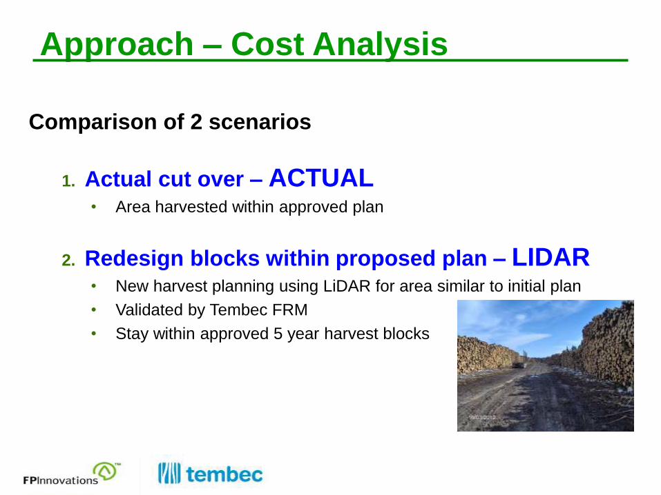
Comparison of 2 scenarios
1. Actual cut over – ACTUAL • Area harvested within approved plan
2. Redesign blocks within proposed plan – LIDAR • New harvest planning using LiDAR for area similar to initial plan
• Validated by Tembec FRM
• Stay within approved 5 year harvest blocks
Approach – Cost Analysis
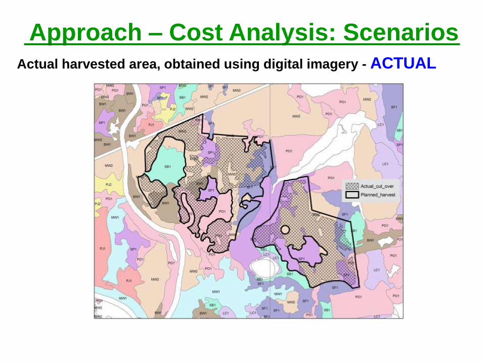
Actual harvested area, obtained using digital imagery - ACTUAL
Approach – Cost Analysis: Scenarios

Actual harvested area, with LiDAR predicted DBHq - ACTUAL
Approach – Cost Analysis: Scenarios
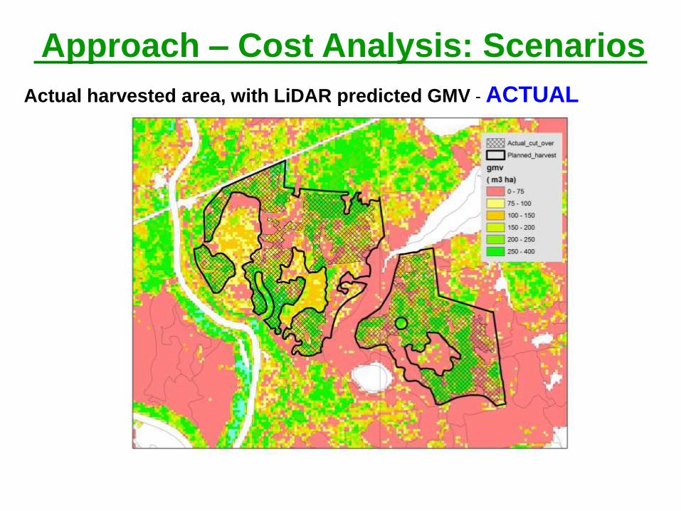
Actual harvested area, with LiDAR predicted GMV - ACTUAL
Approach – Cost Analysis: Scenarios

Redesign plan, based on full suite of LiDAR data products – LIDAR
DBHq (cm) GMV (m3 ha)
Approach – Cost Analysis: Scenarios
ACTUAL LIDAR
Removed area of less
GMV from Scenario

Road segments
not required and
removed from
modeling
Proposed „NEW‟ road network, takes advantage of LiDAR scenarios
Approach – Cost Analysis: Scenarios
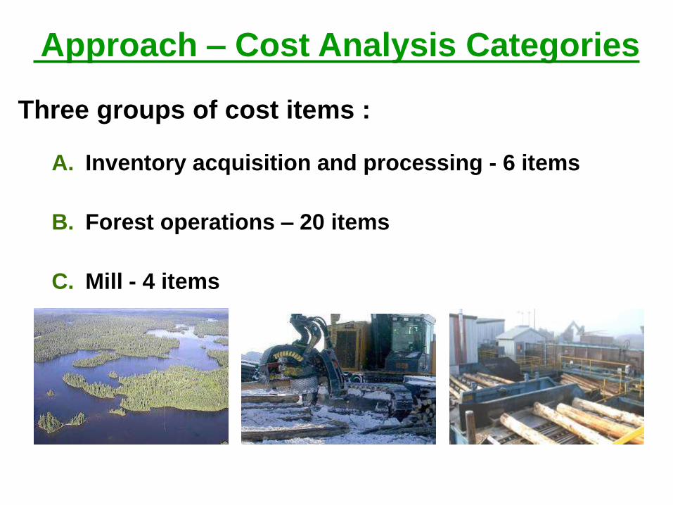
Three groups of cost items :
A. Inventory acquisition and processing - 6 items
B. Forest operations – 20 items
C. Mill - 4 items
Approach – Cost Analysis Categories

B. Forest Operations Cost Analysis Savings
• Forest management plan (FMP) revisions
• Better wood allocation at the planning stage
• Budget forecast
• Decrease of Forest and Mill Inventory
• Better freshness on the wood products
• Feller-buncher productivity (m3/ha)
• Full-tree productivity (m3/stem)
• Skidding productivity
• Wood cutting optimization
• Wood damage on immature wood
• Wood delivery logistics
• Floating costs
• Block layout
• Handling productivity
• Better road location & design
• Road construction
• Road maintenance
• Silviculture funds
• Silviculture cost
• Indirect costs
N/A
$0.13 m3
$0.02 m3
$0.07 m3 m³
$0.09 m3
$0.08 m3
$0.19 m3
$ ???
$ ???
$ ???
$ ???
$0.05 m3
$0.05 m3
$0.02 m3
$0.01 m3
$0.43 m3
$0.03 m3
$0.06 m3
$0.02 m3
$0.15 m3
Total $1.40 m3
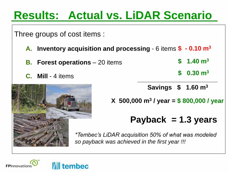
Three groups of cost items :
A. Inventory acquisition and processing - 6 items
B. Forest operations – 20 items
C. Mill - 4 items
$ - 0.10 m3
$ 1.40 m3
$ 0.30 m3
Savings $ 1.60 m3
X 500,000 m3 / year = $ 800,000 / year
Payback = 1.3 years
Results: Actual vs. LiDAR Scenario
*Tembec’s LiDAR acquisition 50% of what was modeled
so payback was achieved in the first year !!!
Ongoing Enhancements
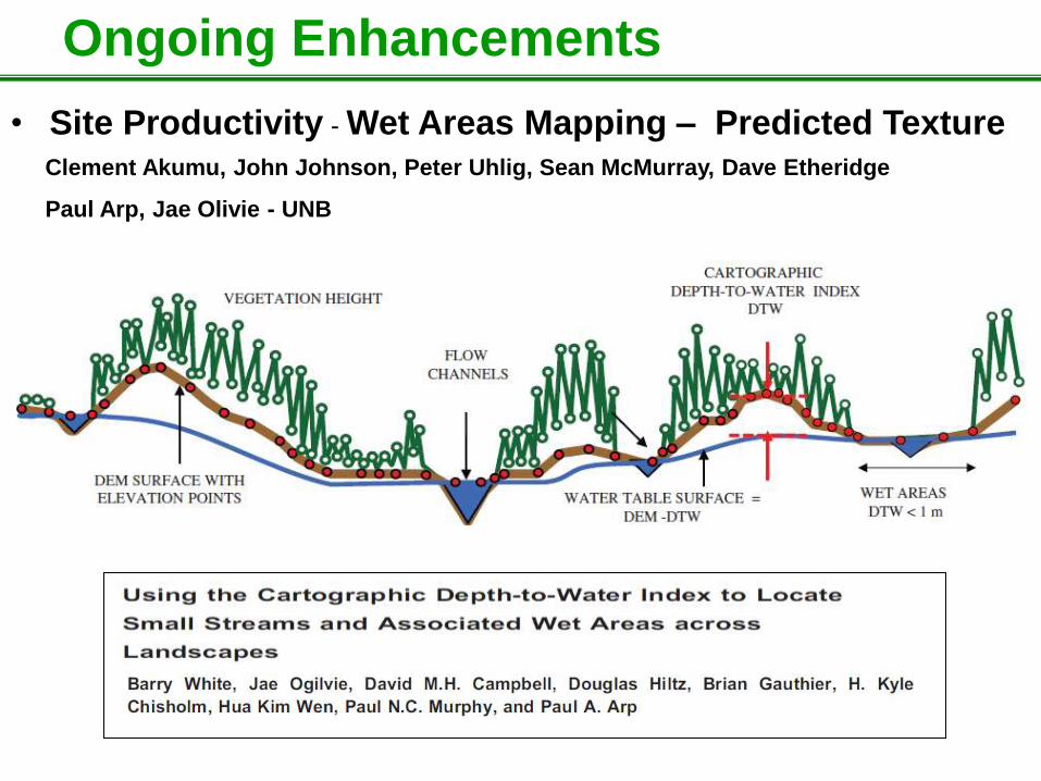
• Site Productivity - Wet Areas Mapping – Predicted Texture
Clement Akumu, John Johnson, Peter Uhlig, Sean McMurray, Dave Etheridge
Paul Arp, Jae Olivie - UNB

Ongoing Enhancements
• Site Productivity - Wet Areas Mapping – Predicted Texture
Clement Akumu, John Johnson, Peter Uhlig, Sean McMurray, Dave Etheridge
Paul Arp, Jae Olivie - UNB
Depth to
Water table
Raster

Ongoing Enhancements
• Site Productivity - Wet Areas Mapping – Predicted Texture
Clement Akumu, John Johnson, Peter Uhlig, Sean McMurray, Dave Etheridge
Environmental input variables:
• Elevation (10m)
• Slope (%)
• Surface shape (Curvature)
• Mode of deposition (NOEGTS)
• Landcover
• Slope Position from TPI
• (macro window = 1km)
• (medium window = 500m)
• (micro window = 20m)
• Wetness Index
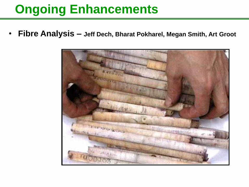
Ongoing Enhancements
• Fibre Analysis – Jeff Dech, Bharat Pokharel, Megan Smith, Art Groot

Ongoing Enhancements
• ITC – Individual Tree Classification

Ongoing Enhancements
Jack Pine - Dbh
y = 1.1364x + 5.945
R2 = 0.8163
0.0
5.0
10.0
15.0
20.0
25.0
30.0
35.0
40.0
45.0
50.0
0 5 10 15 20 25 30 35
Crown Radius * HT
Db
h
cm
Black Spruce - DBH
y = 1.019x + 7.4676
R2 = 0.7241
0.0
5.0
10.0
15.0
20.0
25.0
30.0
35.0
0 5 10 15 20 25
Crown Radius * Ht
DB
H c
m
Jack pine DBH
Black spruce DBH
Crown radius x Height
• ITC – Individual Tree Classification

• Rapid technology evolution – Discrete LiDAR Full Waveform Increased density
– SGM Pixel-correlation methods expanding
– New acquisitions on PRF to pursue next generation inventories – crown attributes – species - stem form – tree quality – fibre properties
SGM 2009 LiDAR 2012 LiDAR 2005
PRF Plot nPW12
Ongoing Enhancements

Future Directions
• Focus shifting towards individual tree modeling
• Imagery analysis techniques improving – slower than LiDAR
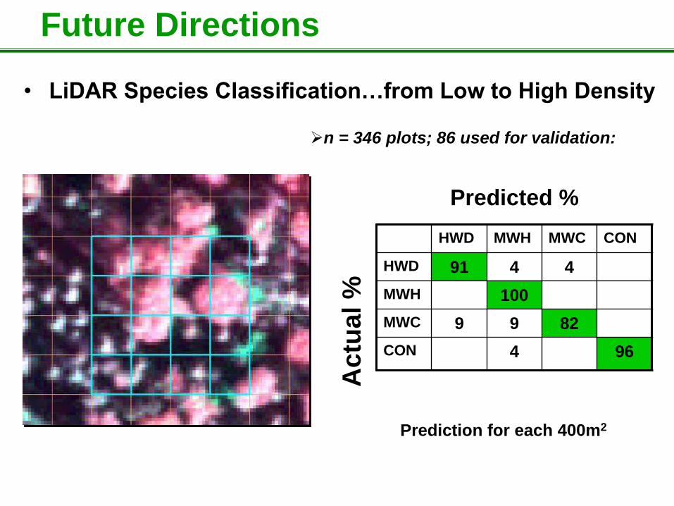
Future Directions
• LiDAR Species Classification…from Low to High Density
n = 346 plots; 86 used for validation:
HWD MWH MWC CON
HWD 91 4 4
MWH 100
MWC 9 9 82
CON 4 96 A
ctu
al
%
Predicted %
Prediction for each 400m2
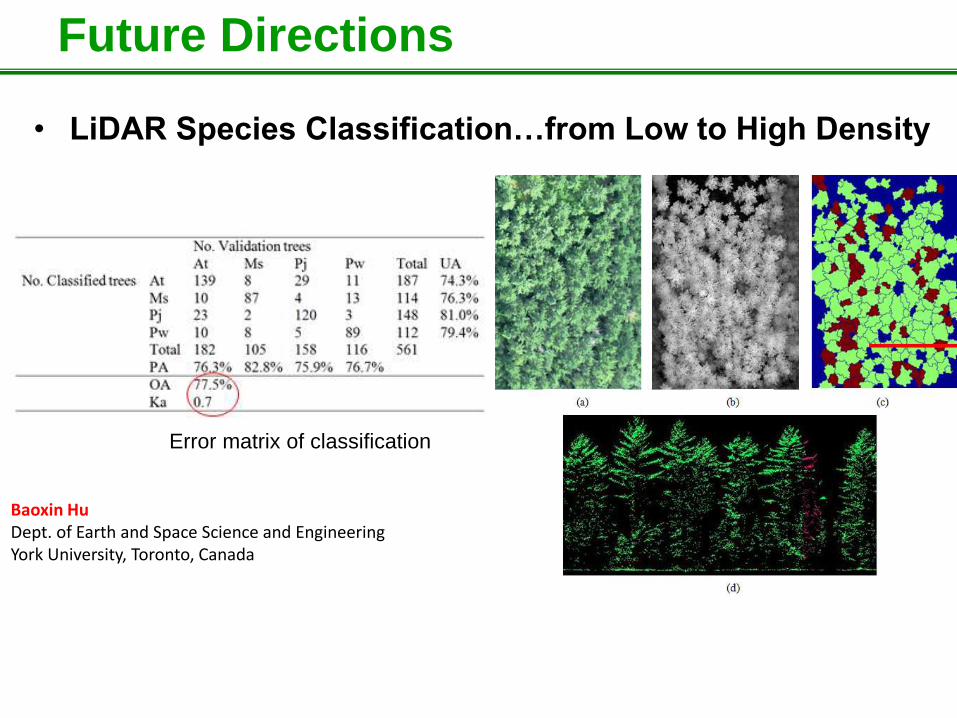
• LiDAR Species Classification…from Low to High Density
Error matrix of classification
Baoxin Hu Dept. of Earth and Space Science and Engineering York University, Toronto, Canada
Future Directions
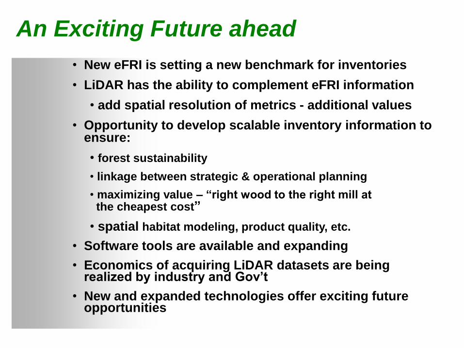
• New eFRI is setting a new benchmark for inventories
• LiDAR has the ability to complement eFRI information
• add spatial resolution of metrics - additional values
• Opportunity to develop scalable inventory information to ensure:
• forest sustainability
• linkage between strategic & operational planning
• maximizing value – “right wood to the right mill at the cheapest cost”
• spatial habitat modeling, product quality, etc.
• Software tools are available and expanding
• Economics of acquiring LiDAR datasets are being realized by industry and Gov’t
• New and expanded technologies offer exciting future opportunities
An Exciting Future ahead

Thank you
Questions?
705 475-5561
705 541-5610
Contact information:

Extra Slides

$0.18 m3 $0.08 m3 Conversion from $/ha to $/m3 based on annual area and harvest levels
A. Acquisition & Processing Cost Analysis
*RMF LIDAR acquisition cost about $0.50/ha
Cost Comparison Items Cost paid by Actual LiDAR
Data acquisition & processing costs $/ha $/ha
LiDAR data acquisition Tembec - 1.00*
LiDAR processing Tembec - 0.45
Lidar validation plots Tembec - 0.15
Photo acquisition Govt 0.46 0.46
Photo processing and interpretation Govt 0.44 0.44
Traditional inventory plots Govt 0.40 0.40
Total $1.30 $2.90
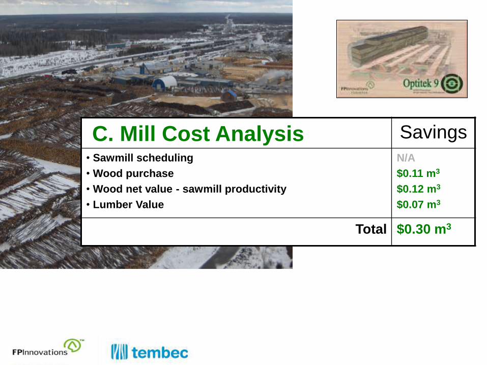
C. Mill Cost Analysis Savings
• Sawmill scheduling
• Wood purchase
• Wood net value - sawmill productivity
• Lumber Value
N/A
$0.11 m3
$0.12 m3
$0.07 m3
Total $0.30 m3

Dry Mesic
Mesic-moist Moist
Slightly waterlogged
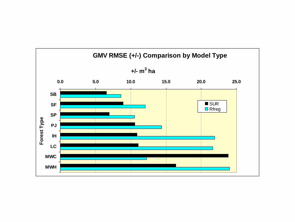
GMV RMSE (+/-) Comparison by Model Type
0.0 5.0 10.0 15.0 20.0 25.0
SB
SF
SP
PJ
IH
LC
MWC
MWH
Fo
res
t T
yp
e
+/- m3 ha
SURRfreg