remote sensing

Article

Operational Drought Monitoring in Kenya UsingMODIS NDVI Time SeriesAnja Klisch and Clement Atzberger *

Institute for Surveying, Remote Sensing and Land Information, University of Natural Resources and LifeSciences (BOKU), Peter Jordan Strasse 82, 1190 Vienna, Austria; anja.klisch@boku.ac.at* Correspondence: clement.atzberger@boku.ac.at; Tel.: +43-1-47654-85701; Fax: +43-1-47654-85742

Academic Editors: Alfredo R. Huete and Prasad S. ThenkabailReceived: 19 January 2016; Accepted: 16 March 2016; Published: 24 March 2016

Abstract: Reliable drought information is of utmost importance for efficient drought management.This paper presents a fully operational processing chain for mapping drought occurrence, extent andstrength based on Moderate Resolution Imaging Spectroradiometer (MODIS) normalized differencevegetation index (NDVI) data at 250 m resolution. Illustrations are provided for the territory of Kenya.The processing chain was developed at BOKU (University of Natural Resources and Life Sciences,Vienna, Austria) and employs a modified Whittaker smoother providing consistent (de-noised)NDVI “Monday-images” in near real-time (NRT), with time lags between zero and thirteen weeks.At a regular seven-day updating interval, the algorithm constrains modeled NDVI values based onreasonable temporal NDVI paths derived from corresponding (multi-year) NDVI “climatologies”.Contrary to other competing approaches, an uncertainty range is produced for each pixel, time stepand time lag. To quantify drought strength, the vegetation condition index (VCI) is calculated atpixel level from the de-noised NDVI data and is spatially aggregated to administrative units. Besidesthe original weekly temporal resolution, the indicator is also aggregated to one- and three-monthlyintervals. During spatial and temporal aggregations, uncertainty information is taken into accountto down-weight less reliable observations. Based on the provided VCI, Kenya’s National DroughtManagement Authority (NDMA) has been releasing disaster contingency funds (DCF) to sustaincounties in drought conditions since 2014. The paper illustrates the successful application of thedrought products within NDMA by providing a retrospective analysis applied to droughts reportedby regular food security assessments. We also present comparisons with alternative products of theUS Agency for International Development (USAID)’s Famine Early Warning Systems Network(FEWS NET). We found an overall good agreement (R2 = 0.89) between the two datasets, butobserved some persistent (seasonal and spatial) differences that should be assessed against externalreference information.

Keywords: vegetation condition index; uncertainty; Whittaker smoother; MODIS; DroughtContingency Funds; NDMA; Kenya

1. Introduction

Drought is a recurrent natural phenomenon in many arid and semi-arid regions of the world [1].Each year it affects millions of the most vulnerable people [2,3]. According to Below et al. [4], morethan 50% of all deaths associated with natural hazards are drought related, and only floods rank higherin terms of the number of people affected.

The stress following a drought depends primarily on the strength, duration, timing and spatialextent of the dry spell. For similar meteorological conditions, different communities and economicsectors show varying vulnerabilities and resiliencies to drought events. Effects differ for example as afunction of available coping strategies and previous (environmental) conditions [5].

Remote Sens. 2016, 8, 267; doi:10.3390/rs8040267 www.mdpi.com/journal/remotesensing

Remote Sens. 2016, 8, 267 2 of 22

Drought definitions and drought indicators are summarized by [1,6]. Satellite observationsprovide synoptic overviews over large areas at dense temporal sampling intervals and are thereforeoften used in drought monitoring systems [7–9]. Reviews of existing satellite-based approaches are forexample found in [5,10]. Several chapters in the recently published compendium “Remote Sensing ofWater Resources, Disasters, and Urban Studies” (edited by Thenkabail) [11] with various aspects oflarge scale drought monitoring in detail [12–15].

For efficient drought management, drought monitoring is essential [16–21]. Especially indrought-prone and vulnerable countries, it is important to continuously monitor droughts and affectedcommunities to prevent disastrous results [22,23]. To enable a quick response, short time lags arerequired between data acquisition and information release.

In 2011, in Kenya, a National Drought Management Authority (NDMA) was established topro-actively manage droughts. NDMA’s mandate is to exercise general supervision and coordinationover all matters relating to drought management within its territory. In 2014, the NDMA receivedDrought Contingency Funds (DCFs) from the European Union (EU) to facilitate early response todrought threats. The DCFs are disbursed by NDMA to drought-affected counties to finance responseactivities that can help mitigating the worst impacts of droughts.

To determine the (agricultural) drought status of a (sub-) county in an objective, reproducibleand cost efficient way, NDMA decided to use Earth Observation (EO) data. For near real-time (NRT)provision of EO data, the University of Natural Resources and Life Sciences (BOKU) developed andimplemented an advanced filtering method for Moderate Resolution Imaging Spectroradiometer(MODIS) normalized difference vegetation index (NDVI) images for NDMA, described below indetail. Numerous alternative filtering methods are available, evaluated in several studies (e.g., [24–29]).In our processing chain, we employ the Whittaker smoother [30], which offers some appropriatecharacteristics for filtering NDVI time series [31–33].

The BOKU processing yields reliable drought indicators at county and sub-county levels forvarious aggregation times and livelihood zones. The image analysis is complemented by field-based(socio-economic) indicators at NDMA as well as satellite-based rainfall estimates from the TAMSATgroup of University of Reading (UK) [34,35]. The innovative DCF disbursement mechanisms of NDMAensure a timely support of drought-affected counties and communities. As DCFs are only disbursed tocounty governments having approved drought mitigation plans, the setting also provides a strongmotivation for drought preparedness activities.

The objective of this paper is to introduce the processing chain implemented for MODIS NDVIdata at BOKU according to the needs of NDMA. We put emphasis on describing the NRT filteringand the provision of uncertainty estimates that are employed for drought anomaly calculation.Through comparison with the well-established data of the US Agency for International Development(USAID)’s Famine Early Warning Systems Network (FEWS NET) [36,37], we highlight and quantifysimilarities and differences between the two datasets. FEWS NET data are used for droughtmonitoring and assessing agricultural production around the globe mainly by the USAID but alsoother organizations (e.g., by World Food Program and FAO) [10,36]. The comparison is interestingbecause the (consolidated) FEWS NET data are only delivered 5–6 weeks after the end of each month,while the BOKU drought indicators are provided in NRT. Hence, our study allows evaluating theimpact of our NRT processing versus the time-lagged indicators provided by FEWS NET. The FEWSNET data, however, do not provide an absolute reference suitable for assessing the quality of theBOKU data.

2. Material and Methods

2.1. Study Area

BOKU’s processing chain, as illustrated in this note, covers an area of 10˝ ˆ 11˝ centered overKenya. Replicates of the algorithm have been implemented to cover the pan-European continent as

Remote Sens. 2016, 8, 267 3 of 22

well as part of Brazil, but will not be presented here. Kenya has been chosen for illustration because ofits operational use of BOKU indicators. The country setting is challenging, as Kenya is characterizedby highly variable land cover, biomass, elevation and rainfall (Figure 1).

Remote Sens. 2016, 8, 267 3 of 22

of its operational use of BOKU indicators. The country setting is challenging, as Kenya is characterized by highly variable land cover, biomass, elevation and rainfall (Figure 1).

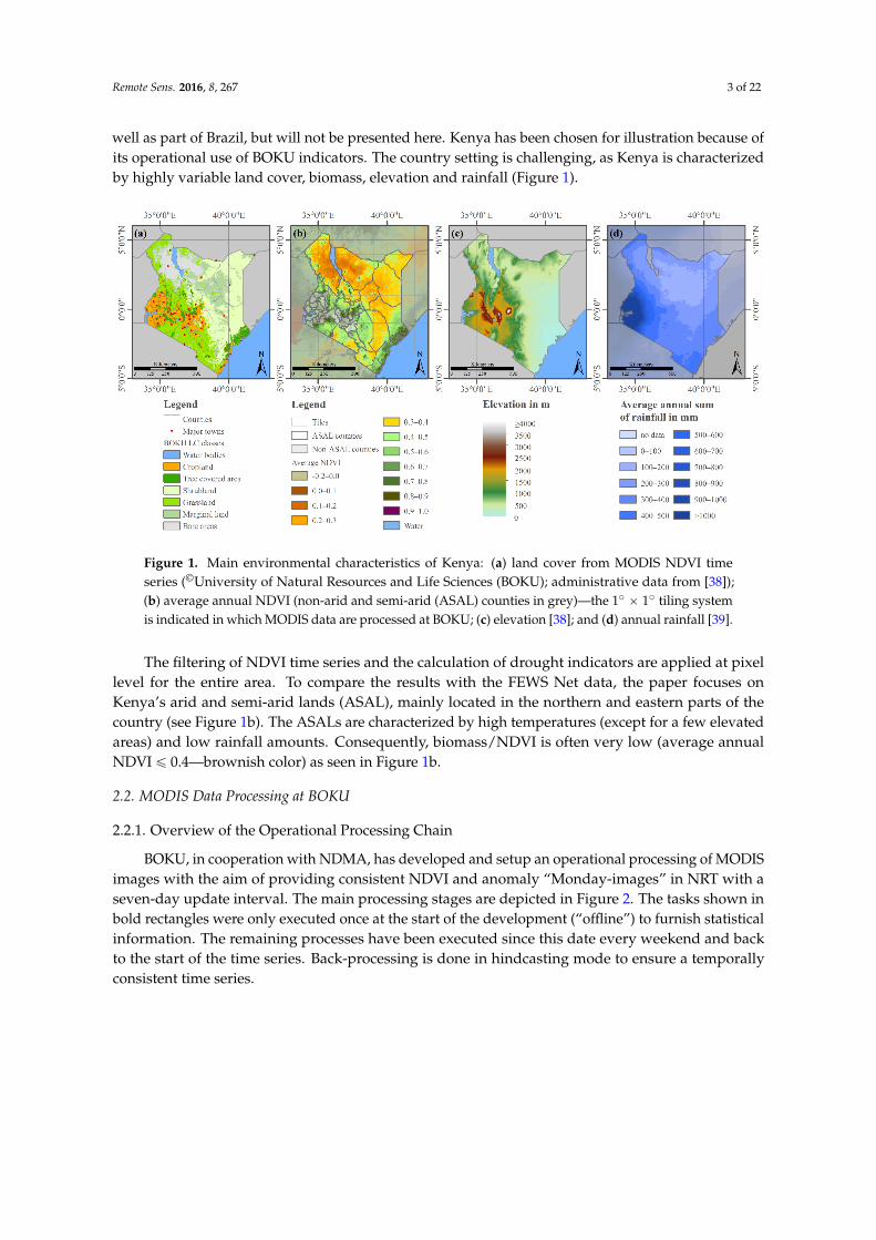
Figure 1. Main environmental characteristics of Kenya: (a) land cover from MODIS NDVI time series (©University of Natural Resources and Life Sciences (BOKU); administrative data from [38]); (b) average annual NDVI (non-arid and semi-arid (ASAL) counties in grey)—the 1° × 1° tiling system is indicated in which MODIS data are processed at BOKU; (c) elevation [38]; and (d) annual rainfall [39].

The filtering of NDVI time series and the calculation of drought indicators are applied at pixel level for the entire area. To compare the results with the FEWS Net data, the paper focuses on Kenya’s arid and semi-arid lands (ASAL), mainly located in the northern and eastern parts of the country (see Figure 1b). The ASALs are characterized by high temperatures (except for a few elevated areas) and low rainfall amounts. Consequently, biomass/NDVI is often very low (average annual NDVI ≤ 0.4—brownish color) as seen in Figure 1b.

2.2. MODIS Data Processing at BOKU

2.2.1. Overview of the Operational Processing Chain

BOKU, in cooperation with NDMA, has developed and setup an operational processing of MODIS images with the aim of providing consistent NDVI and anomaly “Monday-images” in NRT with a seven-day update interval. The main processing stages are depicted in Figure 2. The tasks shown in bold rectangles were only executed once at the start of the development (“offline”) to furnish statistical information. The remaining processes have been executed since this date every weekend and back to the start of the time series. Back-processing is done in hindcasting mode to ensure a temporally consistent time series.

Figure 1. Main environmental characteristics of Kenya: (a) land cover from MODIS NDVI timeseries (©University of Natural Resources and Life Sciences (BOKU); administrative data from [38]);(b) average annual NDVI (non-arid and semi-arid (ASAL) counties in grey)—the 1˝ ˆ 1˝ tiling systemis indicated in which MODIS data are processed at BOKU; (c) elevation [38]; and (d) annual rainfall [39].

The filtering of NDVI time series and the calculation of drought indicators are applied at pixellevel for the entire area. To compare the results with the FEWS Net data, the paper focuses onKenya’s arid and semi-arid lands (ASAL), mainly located in the northern and eastern parts of thecountry (see Figure 1b). The ASALs are characterized by high temperatures (except for a few elevatedareas) and low rainfall amounts. Consequently, biomass/NDVI is often very low (average annualNDVI ď 0.4—brownish color) as seen in Figure 1b.

2.2. MODIS Data Processing at BOKU

2.2.1. Overview of the Operational Processing Chain

BOKU, in cooperation with NDMA, has developed and setup an operational processing of MODISimages with the aim of providing consistent NDVI and anomaly “Monday-images” in NRT with aseven-day update interval. The main processing stages are depicted in Figure 2. The tasks shown inbold rectangles were only executed once at the start of the development (“offline”) to furnish statisticalinformation. The remaining processes have been executed since this date every weekend and backto the start of the time series. Back-processing is done in hindcasting mode to ensure a temporallyconsistent time series.

Remote Sens. 2016, 8, 267 4 of 22Remote Sens. 2016, 8, 267 4 of 22

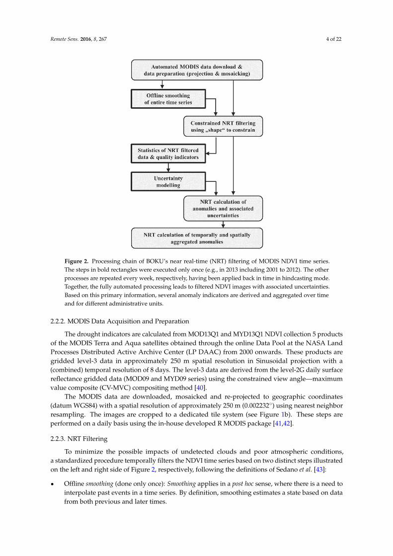
Figure 2. Processing chain of BOKU’s near real-time (NRT) filtering of MODIS NDVI time series. The steps in bold rectangles were executed only once (e.g., in 2013 including 2001 to 2012). The other processes are repeated every week, respectively, having been applied back in time in hindcasting mode. Together, the fully automated processing leads to filtered NDVI images with associated uncertainties. Based on this primary information, several anomaly indicators are derived and aggregated over time and for different administrative units.

2.2.2. MODIS Data Acquisition and Preparation

The drought indicators are calculated from MOD13Q1 and MYD13Q1 NDVI collection 5 products of the MODIS Terra and Aqua satellites obtained through the online Data Pool at the NASA Land Processes Distributed Active Archive Center (LP DAAC) from 2000 onwards. These products are gridded level-3 data in approximately 250 m spatial resolution in Sinusoidal projection with a (combined) temporal resolution of 8 days. The level-3 data are derived from the level-2G daily surface reflectance gridded data (MOD09 and MYD09 series) using the constrained view angle—maximum value composite (CV-MVC) compositing method [40].

The MODIS data are downloaded, mosaicked and re-projected to geographic coordinates (datum WGS84) with a spatial resolution of approximately 250 m (0.002232°) using nearest neighbor resampling. The images are cropped to a dedicated tile system (see Figure 1b). These steps are performed on a daily basis using the in-house developed R MODIS package [41,42].

2.2.3. NRT Filtering

To minimize the possible impacts of undetected clouds and poor atmospheric conditions, a standardized procedure temporally filters the NDVI time series based on two distinct steps illustrated on the left and right side of Figure 2, respectively, following the definitions of Sedano et al. [43]:

• Offline smoothing (done only once): Smoothing applies in a post hoc sense, where there is a need to interpolate past events in a time series. By definition, smoothing estimates a state based on data from both previous and later times.

Figure 2. Processing chain of BOKU’s near real-time (NRT) filtering of MODIS NDVI time series.The steps in bold rectangles were executed only once (e.g., in 2013 including 2001 to 2012). The otherprocesses are repeated every week, respectively, having been applied back in time in hindcasting mode.Together, the fully automated processing leads to filtered NDVI images with associated uncertainties.Based on this primary information, several anomaly indicators are derived and aggregated over timeand for different administrative units.

2.2.2. MODIS Data Acquisition and Preparation

The drought indicators are calculated from MOD13Q1 and MYD13Q1 NDVI collection 5 productsof the MODIS Terra and Aqua satellites obtained through the online Data Pool at the NASA LandProcesses Distributed Active Archive Center (LP DAAC) from 2000 onwards. These products aregridded level-3 data in approximately 250 m spatial resolution in Sinusoidal projection with a(combined) temporal resolution of 8 days. The level-3 data are derived from the level-2G daily surfacereflectance gridded data (MOD09 and MYD09 series) using the constrained view angle—maximumvalue composite (CV-MVC) compositing method [40].

The MODIS data are downloaded, mosaicked and re-projected to geographic coordinates(datum WGS84) with a spatial resolution of approximately 250 m (0.002232˝) using nearest neighborresampling. The images are cropped to a dedicated tile system (see Figure 1b). These steps areperformed on a daily basis using the in-house developed R MODIS package [41,42].

2.2.3. NRT Filtering

To minimize the possible impacts of undetected clouds and poor atmospheric conditions,a standardized procedure temporally filters the NDVI time series based on two distinct steps illustratedon the left and right side of Figure 2, respectively, following the definitions of Sedano et al. [43]:

‚ Offline smoothing (done only once): Smoothing applies in a post hoc sense, where there is a need tointerpolate past events in a time series. By definition, smoothing estimates a state based on datafrom both previous and later times.

Remote Sens. 2016, 8, 267 5 of 22

‚ NRT filtering (repeated every week): Filtering is relevant in an online learning sense, in whichcurrent conditions are to be estimated by the currently available data. Filtering, therefore, involvescalculating the estimate of a certain state based on a partial sequence of inputs.

BOKU’s smoothing step uses the Whittaker smoother, which fits a discrete series to discrete dataand puts a penalty on the roughness of the smooth curve [25,30,32]. It smooths and interpolatesthe data in the historical archive (2001 to 2012) to daily NDVI values. The smoothing takes intoaccount the quality of the observations according to the MODIS VI Quality Assessment Science DataSet (QA SDS) [40] and the compositing day for each pixel. The weights assigned to the MODISobservations based on the QA SDS are reported in Table 1. For a detailed description of the filteringprocedure and settings, see [33]. The original Whittaker smoother is presented in [30].

Table 1. MODIS quality flags (QF) and assigned weights for the Whittaker smoothing and filtering.Observations qualified as “less reliable/unreliable” (e.g., VI usefulness >7) are excluded from thefiltering (weight = 0). VI usefulness values between 4 and 7 (“acceptable”) are linearly scaled between0.8 and 0.2. Observations with values 1–3 are considered to be of “good” or “very good” quality andassigned a weight of one.

MODIS QF Description Weight in Filtering

1 Very good 1.0

2 Good 1.0

3 Good 1.0

4

Acceptable

0.85 0.66 0.47 0.2

8 Less reliable/unreliable 0.0

9 Less reliable/unreliable 0.0

Only every 7th image is stored from the output of the daily NDVI time series, corresponding to“Mondays”. From the smoothed “Monday” images, weekly statistics are calculated describing thetypical NDVI temporal paths for a given location and time (NDVI “climatology”). This informationserves for “constraining” the Whittaker smoother during the NRT filtering (Figure 2).

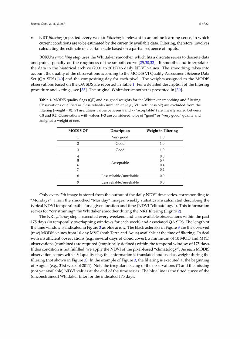
The NRT filtering step is executed every weekend and uses available observations within the past175 days (in temporally overlapping windows for each week) and associated QA SDS. The length ofthe time window is indicated in Figure 3 as blue arrow. The black asterisks in Figure 3 are the observed(raw) MODIS values from 16-day MVC (both Terra and Aqua) available at the time of filtering. To dealwith insufficient observations (e.g., several days of cloud cover), a minimum of 10 MOD and MYDobservations (combined) are required (empirically defined) within the temporal window of 175 days.If this condition is not fulfilled, we apply the NDVI of the pixel-based “climatology”. As each MODISobservation comes with a VI quality flag, this information is translated and used as weight during thefiltering (not shown in Figure 3). In the example of Figure 3, the filtering is executed at the beginningof August (e.g., 31st week of 2011). Note the irregular spacing of the observations (*) and the missing(not yet available) NDVI values at the end of the time series. The blue line is the fitted curve of the(unconstrained) Whittaker filter for the indicated 175 days.

Remote Sens. 2016, 8, 267 6 of 22

Remote Sens. 2016, 8, 267 6 of 22

advantage of observations available to the left and right (e.g., back and forward in time). It serves as a “reference” and for modeling the uncertainty in our processing.

Note that missing constraints in NRT filtering (e.g., at the right side of the smoothing spline) may lead to arbitrary high or low values, particularly at times of the year, when rapid NDVI changes take place and/or many missing or unreliable inputs occur. Thus, we apply a pixel specific constraining procedure that limits the NDVI change between consecutive “Mondays” according to weekly statistics of the offline-smoothed data. In Figure 3, the effect of the constraining is schematically depicted as the difference between the blue line (the unconstrained Whittaker spline) and the (colored) dots. Only the constrained outputs are stored and used for drought mapping in our processing.

Besides the mentioned “Monday” images, BOKU stores a number of metrics characterizing the particular filtering conditions at each filtering step (e.g., each weekend). The various metrics are listed in Table 2 and permit later modeling of the uncertainty of the smoothed outcome. From Figure 3, it can for example be seen that sixteen observations were available in total in the time window of 175 days; the most recent (available) observation at the time of filtering was 33 days old. These and other characteristics are stored.

The NRT processing started in 2014. For processing the data prior to 2014, hindcasting is used (e.g., simulating the incomplete availability of data as experienced in reality). Saving the five output NDVI images, the reference image, plus quality information (Table 2) every weekend allows BOKU to keep a consistent archive of the different consolidation phases while characterizing the filtering conditions for the entire time series starting from 2001. Data are not over-written, as different applications may have different timeliness constraints.

Figure 3. Principle of BOKU’s constrained near real-time (NRT) filtering. The five colored dots are the final (constrained) “Monday” images, representing different consolidation phases (from 0 to 4 weeks).

2.2.4. Uncertainty Modeling

Before starting the operational production of data for NDMA, pre-produced NRT filtered data were compared to the smoothed “reference” time series, where all observations were available (e.g., central black dot in Figure 3). The difference between the “reference” time series and NRT estimates gives the “error” of the NRT filtering. We model this “error” using the stored quality information (Table 2). In our operational setting, the uncertainty of a pixel filtered in NRT is estimated based on those previously established models. This is done independently for each pixel position, output product and time step in NRT. We are not aware of other competing NDVI products providing such uncertainty information (e.g., [24,44–48]).

Figure 3. Principle of BOKU’s constrained near real-time (NRT) filtering. The five colored dots are thefinal (constrained) “Monday” images, representing different consolidation phases (from 0 to 4 weeks).

The output of the weekly NRT filtering is six images, indicated as colored/black dots in Figure 3,representing different consolidation phases of the filtered NDVI (“output 1” to “output 4”). Obviously,“output 4” is more reliable (e.g., better constrained through available data) compared to the “output 0”,which is always extrapolated as MODIS observations are not available in real time. Producing filtereddata in NRT avoids time lags related to the otherwise necessary consolidation period (e.g., 5–6 weekswith FEWS NET data).

The sixth and final image stored every weekend corresponds to the black dot in Figure 3.Obviously, this fully smoothed value will become available only after thirteen weeks but has theadvantage of observations available to the left and right (e.g., back and forward in time). It serves as a“reference” and for modeling the uncertainty in our processing.

Note that missing constraints in NRT filtering (e.g., at the right side of the smoothing spline) maylead to arbitrary high or low values, particularly at times of the year, when rapid NDVI changes takeplace and/or many missing or unreliable inputs occur. Thus, we apply a pixel specific constrainingprocedure that limits the NDVI change between consecutive “Mondays” according to weekly statisticsof the offline-smoothed data. In Figure 3, the effect of the constraining is schematically depicted as thedifference between the blue line (the unconstrained Whittaker spline) and the (colored) dots. Only theconstrained outputs are stored and used for drought mapping in our processing.

Besides the mentioned “Monday” images, BOKU stores a number of metrics characterizing theparticular filtering conditions at each filtering step (e.g., each weekend). The various metrics are listedin Table 2 and permit later modeling of the uncertainty of the smoothed outcome. From Figure 3,it can for example be seen that sixteen observations were available in total in the time window of175 days; the most recent (available) observation at the time of filtering was 33 days old. These andother characteristics are stored.

Remote Sens. 2016, 8, 267 7 of 22

Table 2. Quality and pixel information stored during near real-time filtering per “Monday image”.

Name Description

Days to last measurement (NLM) Number of days to last available measurementQuality of last measurement (QLM) MODIS VI quality of last available measurementNumber of measurements (NWM) Number of valid measurements within the time window (175 days)

Quality of measurements (QWM) Average MODIS VI quality of valid measurements within the timewindow (175 days)

The NRT processing started in 2014. For processing the data prior to 2014, hindcasting is used(e.g., simulating the incomplete availability of data as experienced in reality). Saving the five outputNDVI images, the reference image, plus quality information (Table 2) every weekend allows BOKU tokeep a consistent archive of the different consolidation phases while characterizing the filteringconditions for the entire time series starting from 2001. Data are not over-written, as differentapplications may have different timeliness constraints.

2.2.4. Uncertainty Modeling

Before starting the operational production of data for NDMA, pre-produced NRT filtered datawere compared to the smoothed “reference” time series, where all observations were available (e.g.,central black dot in Figure 3). The difference between the “reference” time series and NRT estimatesgives the “error” of the NRT filtering. We model this “error” using the stored quality information(Table 2). In our operational setting, the uncertainty of a pixel filtered in NRT is estimated basedon those previously established models. This is done independently for each pixel position, outputproduct and time step in NRT. We are not aware of other competing NDVI products providing suchuncertainty information (e.g., [24,44–48]).

2.3. Drought Indicator Calculation

From the filtered NDVI datasets, temporally and spatially aggregated vegetation condition index(VCI) anomalies [49] are calculated. Conceptionally, the VCI enhances the inter-annual variationsof a vegetation index (e.g., NDVI) in response to weather fluctuations while reducing the impactof ecosystem specific response (e.g., driven by climate, soils, vegetation type and topography) [49].At BOKU, a weekly VCI is calculated at pixel level from the filtered NDVI data (each consolidationphase separately—not specified in Equation (1)) using

VCIi “ 100ˆpNDVIi´NDVImin,iq{pNDVImax,i´NDVImin,iq (1)

where VCIi is the vegetation condition index at time step i, NDVIi is the filtered normalized differencevegetation index observed at time step i and NDVImin,i/NDVImax,i are the lowest/highest seven-dayfiltered NDVI values observed from 2003 to 2012 at week i.

In a very similar way, z-score values (ZVI) are calculated (Equation (2))

ZVIi “ pNDVIi´NDVImean,iq{stdpNDVIiq (2)

where ZVIi is the standard score (z-score) of NDVI at time step i, NDVIi is the filtered NDVI observedat time step i, NDVImean,i are the average seven-day filtered NDVI values (between 2003 and 2012) atweek i and std(NDVIi) is the standard deviation of seven-day filtered NDVI values (2003 to 2012) atweek i.

The VCI puts an actual NDVI value in a range between historical minimum (VCI = 0%) andmaximum (VCI = 100%). ZVI indicates the (signed) number of standard deviations an observationis above/below the mean. Results for ZVI are not covered in this paper due to their high correlationwith VCI (not shown).

Remote Sens. 2016, 8, 267 8 of 22

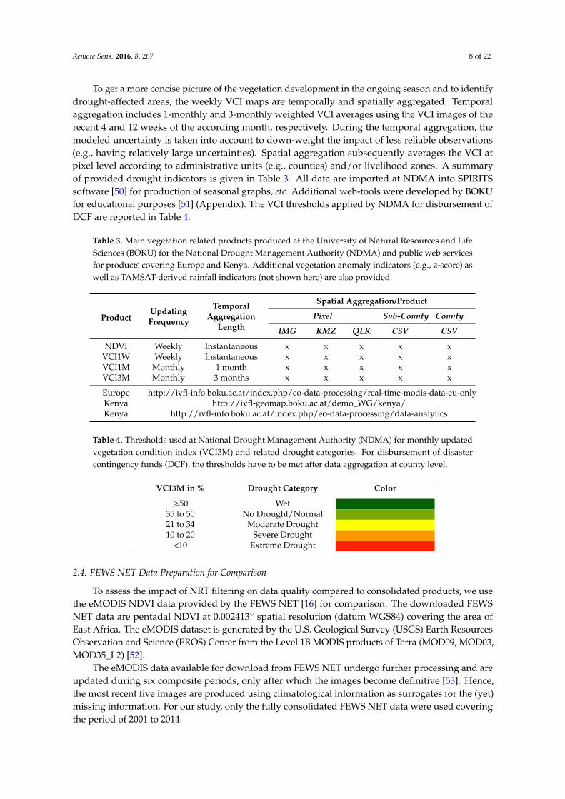
To get a more concise picture of the vegetation development in the ongoing season and to identifydrought-affected areas, the weekly VCI maps are temporally and spatially aggregated. Temporalaggregation includes 1-monthly and 3-monthly weighted VCI averages using the VCI images of therecent 4 and 12 weeks of the according month, respectively. During the temporal aggregation, themodeled uncertainty is taken into account to down-weight the impact of less reliable observations(e.g., having relatively large uncertainties). Spatial aggregation subsequently averages the VCI atpixel level according to administrative units (e.g., counties) and/or livelihood zones. A summaryof provided drought indicators is given in Table 3. All data are imported at NDMA into SPIRITSsoftware [50] for production of seasonal graphs, etc. Additional web-tools were developed by BOKUfor educational purposes [51] (Appendix). The VCI thresholds applied by NDMA for disbursement ofDCF are reported in Table 4.

Table 3. Main vegetation related products produced at the University of Natural Resources and LifeSciences (BOKU) for the National Drought Management Authority (NDMA) and public web servicesfor products covering Europe and Kenya. Additional vegetation anomaly indicators (e.g., z-score) aswell as TAMSAT-derived rainfall indicators (not shown here) are also provided.

ProductUpdatingFrequency

TemporalAggregation

Length

Spatial Aggregation/Product

Pixel Sub-County County

IMG KMZ QLK CSV CSV

NDVI Weekly Instantaneous x x x x xVCI1W Weekly Instantaneous x x x x xVCI1M Monthly 1 month x x x x xVCI3M Monthly 3 months x x x x x

Europe http://ivfl-info.boku.ac.at/index.php/eo-data-processing/real-time-modis-data-eu-onlyKenya http://ivfl-geomap.boku.ac.at/demo_WG/kenya/Kenya http://ivfl-info.boku.ac.at/index.php/eo-data-processing/data-analytics

Table 4. Thresholds used at National Drought Management Authority (NDMA) for monthly updatedvegetation condition index (VCI3M) and related drought categories. For disbursement of disastercontingency funds (DCF), the thresholds have to be met after data aggregation at county level.

VCI3M in % Drought Category Color

ě50 Wet35 to 50 No Drought/Normal21 to 34 Moderate Drought10 to 20 Severe Drought

<10 Extreme Drought

2.4. FEWS NET Data Preparation for Comparison

To assess the impact of NRT filtering on data quality compared to consolidated products, we usethe eMODIS NDVI data provided by the FEWS NET [16] for comparison. The downloaded FEWSNET data are pentadal NDVI at 0.002413˝ spatial resolution (datum WGS84) covering the area ofEast Africa. The eMODIS dataset is generated by the U.S. Geological Survey (USGS) Earth ResourcesObservation and Science (EROS) Center from the Level 1B MODIS products of Terra (MOD09, MOD03,MOD35_L2) [52].

The eMODIS data available for download from FEWS NET undergo further processing and areupdated during six composite periods, only after which the images become definitive [53]. Hence,the most recent five images are produced using climatological information as surrogates for the (yet)missing information. For our study, only the fully consolidated FEWS NET data were used coveringthe period of 2001 to 2014.

Remote Sens. 2016, 8, 267 9 of 22

To derive vegetation anomalies from the FEWS NET data, the NDVI images were processed in asimilar way as the BOKU data including five steps:

‚ cropping and resampling to the BOKU grid (see Figure 1b);‚ calculation of pentadal statistics (minimum, maximum) from the NDVI for each pixel and the

period of 2003 to 2012;‚ calculation of pentadal VCI images using the derived statistics (Equation (1));‚ temporal aggregation of VCI images (1 and 3 months) by averaging 6 and 18 pentades,

respectively; and‚ spatial aggregation by averaging according to administrative units (e.g., ASAL counties of Kenya;

see Figure 1b).

3. Results and Discussion

3.1. Illustration of Filtering Performance & Example Products from BOKU

3.1.1. Filtered NDVI Data and Modeled Uncertainty

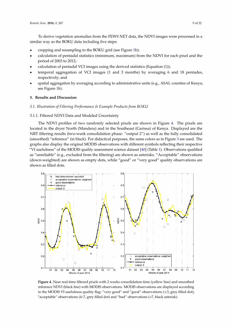
The NDVI profiles of two randomly selected pixels are shown in Figure 4. The pixels arelocated in the dryer North (Mandera) and in the Southeast (Garissa) of Kenya. Displayed are theNRT filtering results (two-week consolidation phase: “output 2”) as well as the fully consolidated(smoothed) “reference” (in black). For didactical purposes, the same colors as in Figure 3 are used. Thegraphs also display the original MODIS observations with different symbols reflecting their respective“VI usefulness” of the MODIS quality assessment science dataset [40] (Table 1). Observations qualifiedas “unreliable” (e.g., excluded from the filtering) are shown as asterisks. “Acceptable” observations(down-weighted) are shown as empty dots, while “good” or “very good” quality observations areshown as filled dots.

Remote Sens. 2016, 8, 267 9 of 22

3. Results and Discussion

3.1. Illustration of Filtering Performance & Example Products from BOKU

3.1.1. Filtered NDVI Data and Modeled Uncertainty

The NDVI profiles of two randomly selected pixels are shown in Figure 4. The pixels are located in the dryer North (Mandera) and in the Southeast (Garissa) of Kenya. Displayed are the NRT filtering results (two-week consolidation phase: “output 2”) as well as the fully consolidated (smoothed) “reference” (in black). For didactical purposes, the same colors as in Figure 3 are used. The graphs also display the original MODIS observations with different symbols reflecting their respective “VI usefulness” of the MODIS quality assessment science dataset [40] (Table 1). Observations qualified as “unreliable” (e.g., excluded from the filtering) are shown as asterisks. “Acceptable” observations (down-weighted) are shown as empty dots, while “good” or “very good” quality observations are shown as filled dots.

Despite the missing and sometimes unreliable observations at the time of filtering, the NRT NDVI profile (yellow) follows quite closely the reference profile (in black), which represents the smoothed outcome if all NDVI observations (before and after a given date) were available. For both pixels, one observes two distinct cycles related to the long and short rains. Abrupt changes of the NDVI profile for the NRT product result from the (sudden) availability of observations at the time of the NRT filtering from one week to the other. The slight delay in the yellow curve with respect to the black curve is a direct result of the not yet available information, which can obviously not be perfectly predicted using the implemented constraining procedure. The graphs also confirm that the MODIS QA SDS flags (e.g., “VI usefulness”) are not always correct [54]. For example, several doubtful “good” or “acceptable” observations can be seen (filled and empty dots), while the only excluded observation (*) in Figure 4 (left) falls exactly into the black curve. Such (presumably) erroneous information has a negative impact on the results of the filtering.

Figure 4. Near real-time filtered pixels with 2 weeks consolidation time (yellow line) and smoothed reference NDVI (black line) with MODIS observations. MODIS observations are displayed according to the MODIS VI usefulness quality flag: “very good” and “good” observations (≤3, grey filled dot), “acceptable” observations (4–7, grey filled dot) and “bad” observations (>7, black asterisk).

Figure 4. Near real-time filtered pixels with 2 weeks consolidation time (yellow line) and smoothedreference NDVI (black line) with MODIS observations. MODIS observations are displayed accordingto the MODIS VI usefulness quality flag: “very good” and “good” observations (ď3, grey filled dot),“acceptable” observations (4–7, grey filled dot) and “bad” observations (>7, black asterisk).

Remote Sens. 2016, 8, 267 10 of 22

Despite the missing and sometimes unreliable observations at the time of filtering, the NRT NDVIprofile (yellow) follows quite closely the reference profile (in black), which represents the smoothedoutcome if all NDVI observations (before and after a given date) were available. For both pixels, oneobserves two distinct cycles related to the long and short rains. Abrupt changes of the NDVI profile forthe NRT product result from the (sudden) availability of observations at the time of the NRT filteringfrom one week to the other. The slight delay in the yellow curve with respect to the black curve is adirect result of the not yet available information, which can obviously not be perfectly predicted usingthe implemented constraining procedure. The graphs also confirm that the MODIS QA SDS flags(e.g., “VI usefulness”) are not always correct [54]. For example, several doubtful “good” or “acceptable”observations can be seen (filled and empty dots), while the only excluded observation (*) in Figure 4(left) falls exactly into the black curve. Such (presumably) erroneous information has a negative impacton the results of the filtering.

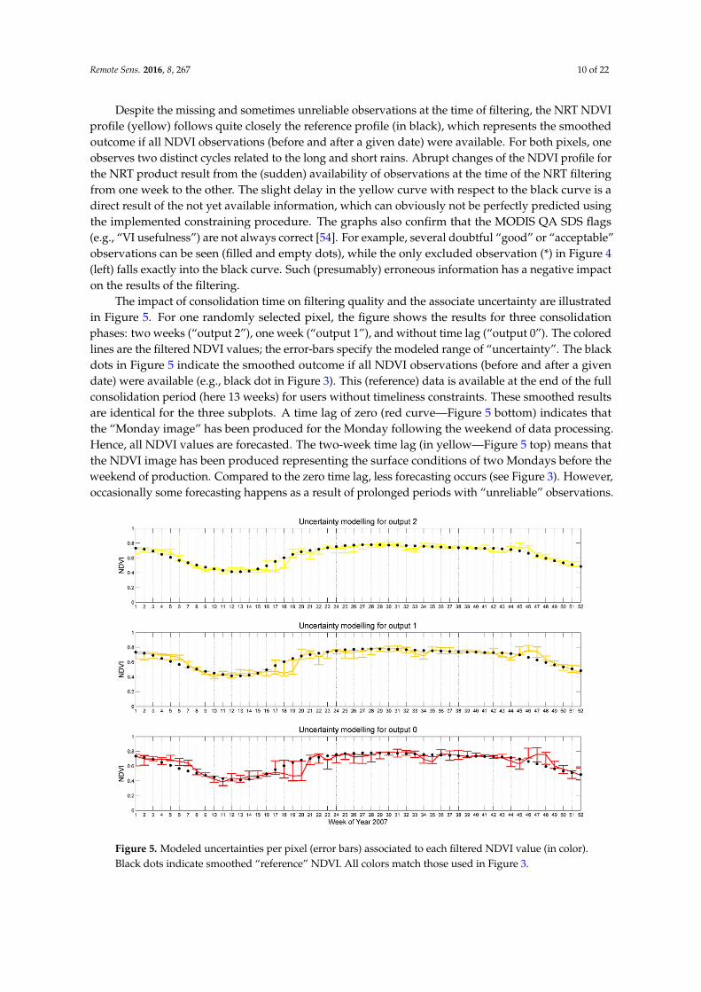
The impact of consolidation time on filtering quality and the associate uncertainty are illustratedin Figure 5. For one randomly selected pixel, the figure shows the results for three consolidationphases: two weeks (“output 2”), one week (“output 1”), and without time lag (“output 0”). The coloredlines are the filtered NDVI values; the error-bars specify the modeled range of “uncertainty”. The blackdots in Figure 5 indicate the smoothed outcome if all NDVI observations (before and after a givendate) were available (e.g., black dot in Figure 3). This (reference) data is available at the end of the fullconsolidation period (here 13 weeks) for users without timeliness constraints. These smoothed resultsare identical for the three subplots. A time lag of zero (red curve—Figure 5 bottom) indicates thatthe “Monday image” has been produced for the Monday following the weekend of data processing.Hence, all NDVI values are forecasted. The two-week time lag (in yellow—Figure 5 top) means thatthe NDVI image has been produced representing the surface conditions of two Mondays before theweekend of production. Compared to the zero time lag, less forecasting occurs (see Figure 3). However,occasionally some forecasting happens as a result of prolonged periods with “unreliable” observations.

Remote Sens. 2016, 8, 267 10 of 22

The impact of consolidation time on filtering quality and the associate uncertainty are illustrated in Figure 5. For one randomly selected pixel, the figure shows the results for three consolidation phases: two weeks (“output 2”), one week (“output 1”), and without time lag (“output 0”). The colored lines are the filtered NDVI values; the error-bars specify the modeled range of “uncertainty”. The black dots in Figure 5 indicate the smoothed outcome if all NDVI observations (before and after a given date) were available (e.g., black dot in Figure 3). This (reference) data is available at the end of the full consolidation period (here 13 weeks) for users without timeliness constraints. These smoothed results are identical for the three subplots. A time lag of zero (red curve—Figure 5 bottom) indicates that the “Monday image” has been produced for the Monday following the weekend of data processing. Hence, all NDVI values are forecasted. The two-week time lag (in yellow—Figure 5 top) means that the NDVI image has been produced representing the surface conditions of two Mondays before the weekend of production. Compared to the zero time lag, less forecasting occurs (see Figure 3). However, occasionally some forecasting happens as a result of prolonged periods with “unreliable” observations.

Figure 5. Modeled uncertainties per pixel (error bars) associated to each filtered NDVI value (in color). Black dots indicate smoothed “reference” NDVI. All colors match those used in Figure 3.

The aim of the NRT filtering is to come as close as possible to the smoothed (e.g., perfectly modeled) outcome. Where this is not possible, the smoothed value should be at least within the modeled uncertainty range. The modeled uncertainty range itself should reflect the modeling conditions—that is the spatially and temporally varying availability and quality of observations. Looking at Figure 5, the following points are interesting to note and confirm that the previously mentioned requirements were met:

• Filtered values (colored lines) become smoother and come closer to the smoothed values (black dots) with increasing consolidation period.

• The modeled uncertainties are of variable widths but generally shrink with increasing consolidation period.

• Occurrences of large differences between filtered and smoothed NDVI values are mostly associated with larger uncertainty ranges.

• In most cases, smoothed values are found within the predicted uncertainty range.

Figure 5. Modeled uncertainties per pixel (error bars) associated to each filtered NDVI value (in color).Black dots indicate smoothed “reference” NDVI. All colors match those used in Figure 3.

Remote Sens. 2016, 8, 267 11 of 22

The aim of the NRT filtering is to come as close as possible to the smoothed (e.g., perfectly modeled)outcome. Where this is not possible, the smoothed value should be at least within the modeleduncertainty range. The modeled uncertainty range itself should reflect the modeling conditions—thatis the spatially and temporally varying availability and quality of observations. Looking at Figure 5,the following points are interesting to note and confirm that the previously mentioned requirementswere met:

‚ Filtered values (colored lines) become smoother and come closer to the smoothed values (blackdots) with increasing consolidation period.

‚ The modeled uncertainties are of variable widths but generally shrink with increasingconsolidation period.

‚ Occurrences of large differences between filtered and smoothed NDVI values are mostly associatedwith larger uncertainty ranges.

‚ In most cases, smoothed values are found within the predicted uncertainty range.

Note that all data from all consolidation periods are stored and produced in a fully consistentmanner in hindcasting mode and this from the beginning of the MODIS time series (2001). Hence, theuser is free to choose his/her product of preference. In some cases, the user might opt for the NRTproduct with the highest quality if he/she does not mind using 3–4 weeks “old” data (e.g., for landcover classifications). In other applications, the user requests more actual information and is thereforewilling to accept less accurate information (and in particular if he/she gets additional information—bypixel—about the modeled uncertainty range).

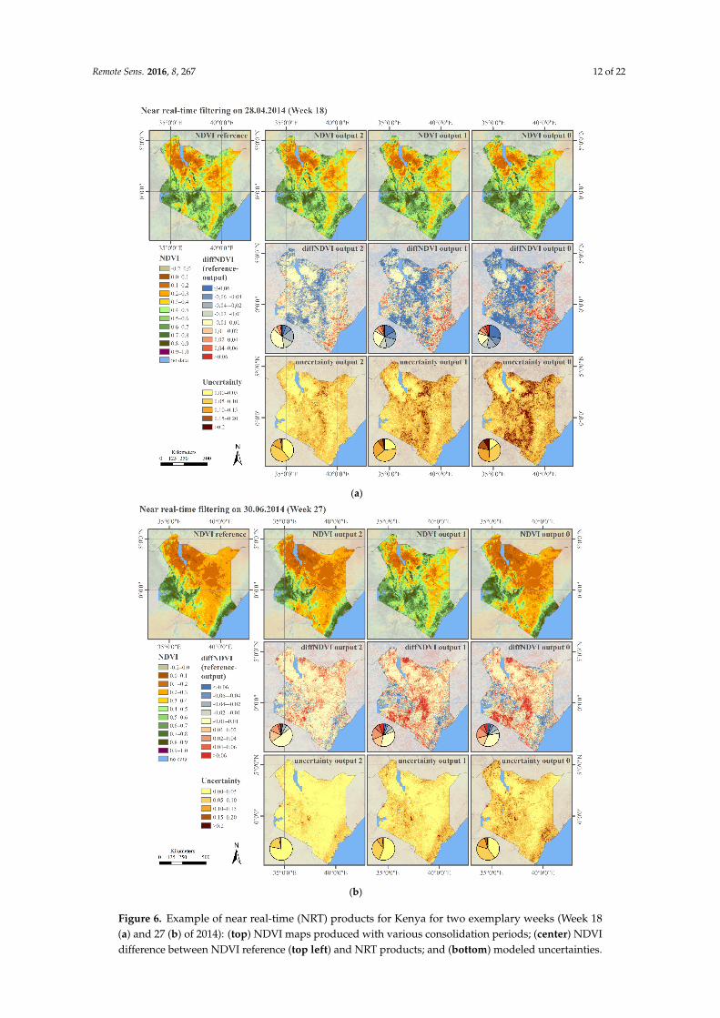
The various consolidation periods and associated uncertainties are combined to derive one- andthree-monthly VCI (Equation (1)) within the NDMA drought monitoring application. The one-monthlyVCI, for example, is calculated by combining the data from the consolidation periods “output 0” to“output 3” (e.g., past four weeks) and hereby take into account the respective uncertainty ranges.In other words, the impact of the newest image (usually with the highest uncertainty range) willgenerally be smaller, compared to the somewhat older (better consolidated) data. A spatial comparisonbetween smoothed and filtered data is shown in Figure 6a (last week of April 2014) and Figure 6b(last week of June 2014).

In the top left hand corner of Figure 6a,b, the NDVI map of the smoothed “reference” (e.g., blackdot in Figure 3) is shown (e.g., best possible result); right to this map are the filtered products withzero to two weeks consolidation period. Thereunder, the NDVI deviations between the smoothedresult and the various filtered versions and the modeled uncertainties are shown. Note that all data arecontinuous and have been put into classes only for illustration purposes. The small inlets (pie charts inFigure 6a,b) represent the respective proportions calculated over the displayed area.

Overall a good agreement can be noted (first row). The differences between the smoothedand the filtered data decrease with increasing consolidation time (e.g., from right to left; secondrow). Spatio-temporally varying pattern of agreement and disagreement (over- and underestimation)depending on the local observation conditions (see Table 2) are also visible from Figure 6a,b. Again,areas with larger deviations (positive or negative) are generally correctly reflected in the modeleduncertainty range (third row).

3.1.2. Calculated Drought Indicators

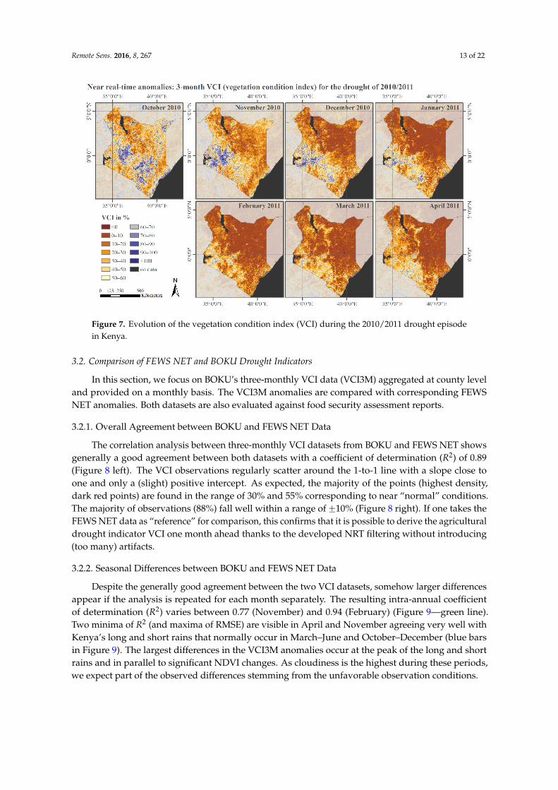
At the beginning of 2011, Kenya experienced one of the most severe droughts in its history,affecting large parts of the country and all ASAL counties. The onset, peak and end of the droughtepisode are illustrated in Figure 7. It displays the three-monthly VCI products from October 2010 toApril 2011. The seven maps depict the timing, strength, location, extent and duration of the drought asobserved in NRT by the BOKU processing chain. Such information proved very valuable to NDMAover the past few years since the start of the service (pers. communication Luigi Luminari—NDMAKenya) as it is provided in NRT, and down-weighting less reliable observations.

Remote Sens. 2016, 8, 267 12 of 22

Remote Sens. 2016, 8, 267 11 of 22

Note that all data from all consolidation periods are stored and produced in a fully consistent manner in hindcasting mode and this from the beginning of the MODIS time series (2001). Hence, the user is free to choose his/her product of preference. In some cases, the user might opt for the NRT product with the highest quality if he/she does not mind using 3–4 weeks “old” data (e.g., for land cover classifications). In other applications, the user requests more actual information and is therefore willing to accept less accurate information (and in particular if he/she gets additional information—by pixel—about the modeled uncertainty range).

The various consolidation periods and associated uncertainties are combined to derive one- and three-monthly VCI (Equation (1)) within the NDMA drought monitoring application. The one-monthly VCI, for example, is calculated by combining the data from the consolidation periods “output 0” to “output 3” (e.g., past four weeks) and hereby take into account the respective uncertainty ranges. In other words, the impact of the newest image (usually with the highest uncertainty range) will generally be smaller, compared to the somewhat older (better consolidated) data. A spatial comparison between smoothed and filtered data is shown in Figure 6a (last week of April 2014) and Figure 6b (last week of June 2014).

(a)

Figure 6. Cont.

Remote Sens. 2016, 8, 267 12 of 22

(b)

Figure 6. Example of near real-time (NRT) products for Kenya for two exemplary weeks (Week 18 (a) and 27 (b) of 2014): (top) NDVI maps produced with various consolidation periods; (center) NDVI difference between NDVI reference (top left) and NRT products; and (bottom) modeled uncertainties.

In the top left hand corner of Figure 6a,b, the NDVI map of the smoothed “reference” (e.g., black dot in Figure 3) is shown (e.g., best possible result); right to this map are the filtered products with zero to two weeks consolidation period. Thereunder, the NDVI deviations between the smoothed result and the various filtered versions and the modeled uncertainties are shown. Note that all data are continuous and have been put into classes only for illustration purposes. The small inlets (pie charts in Figure 6a,b) represent the respective proportions calculated over the displayed area.

Overall a good agreement can be noted (first row). The differences between the smoothed and the filtered data decrease with increasing consolidation time (e.g., from right to left; second row). Spatio-temporally varying pattern of agreement and disagreement (over- and underestimation) depending on the local observation conditions (see Table 2) are also visible from Figure 6a,b. Again, areas with larger deviations (positive or negative) are generally correctly reflected in the modeled uncertainty range (third row).

3.1.2. Calculated Drought Indicators

At the beginning of 2011, Kenya experienced one of the most severe droughts in its history, affecting large parts of the country and all ASAL counties. The onset, peak and end of the drought episode are illustrated in Figure 7. It displays the three-monthly VCI products from October 2010 to April 2011. The seven maps depict the timing, strength, location, extent and duration of the drought as observed in NRT by the BOKU processing chain. Such information proved very valuable to NDMA

Figure 6. Example of near real-time (NRT) products for Kenya for two exemplary weeks (Week 18(a) and 27 (b) of 2014): (top) NDVI maps produced with various consolidation periods; (center) NDVIdifference between NDVI reference (top left) and NRT products; and (bottom) modeled uncertainties.

Remote Sens. 2016, 8, 267 13 of 22

Remote Sens. 2016, 8, 267 13 of 22

over the past few years since the start of the service (pers. communication Luigi Luminari—NDMA Kenya) as it is provided in NRT, and down-weighting less reliable observations.

Figure 7. Evolution of the vegetation condition index (VCI) during the 2010/2011 drought episode in Kenya.

3.2. Comparison of FEWS NET and BOKU Drought Indicators

In this section, we focus on BOKU’s three-monthly VCI data (VCI3M) aggregated at county level and provided on a monthly basis. The VCI3M anomalies are compared with corresponding FEWS NET anomalies. Both datasets are also evaluated against food security assessment reports.

3.2.1. Overall Agreement between BOKU and FEWS NET Data

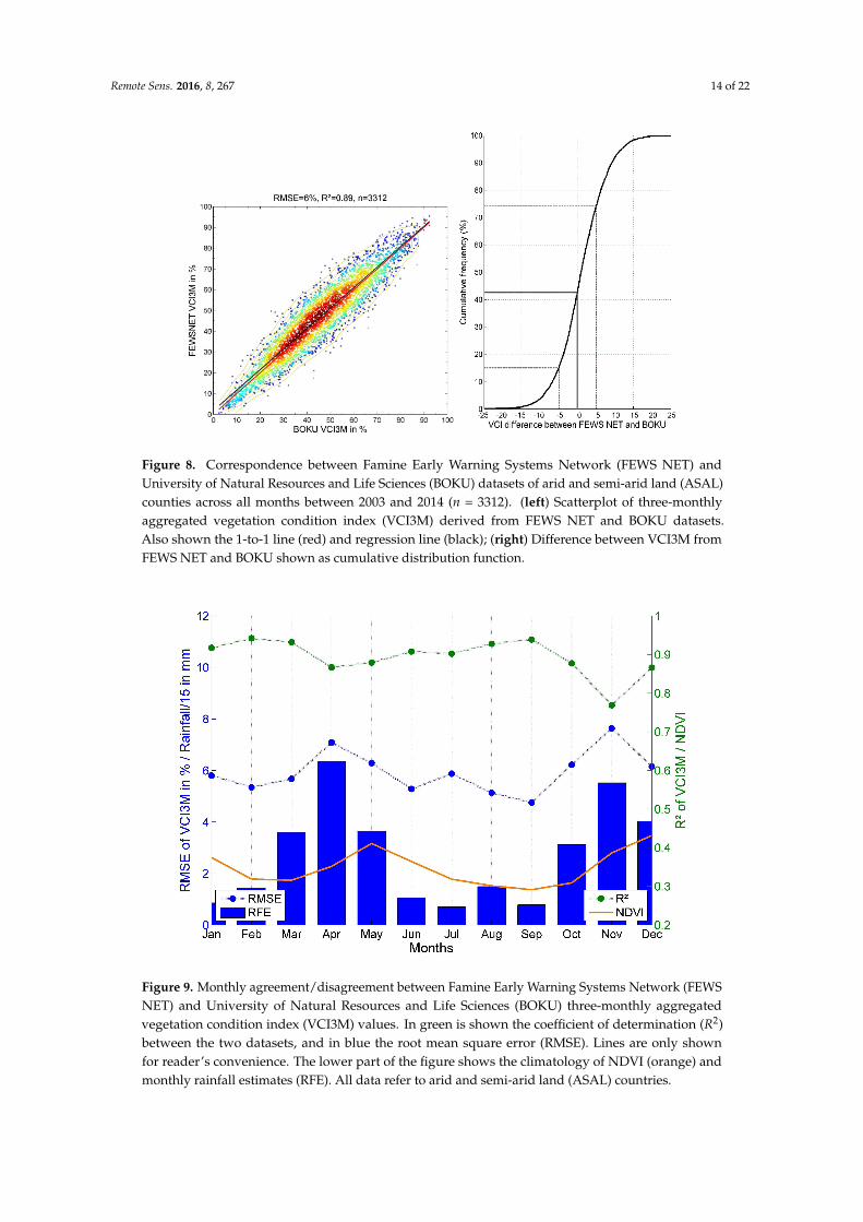
The correlation analysis between three-monthly VCI datasets from BOKU and FEWS NET shows generally a good agreement between both datasets with a coefficient of determination (R2) of 0.89 (Figure 8 left). The VCI observations regularly scatter around the 1-to-1 line with a slope close to one and only a (slight) positive intercept. As expected, the majority of the points (highest density, dark red points) are found in the range of 30% and 55% corresponding to near “normal” conditions. The majority of observations (88%) fall well within a range of ±10% (Figure 8 right). If one takes the FEWS NET data as “reference” for comparison, this confirms that it is possible to derive the agricultural drought indicator VCI one month ahead thanks to the developed NRT filtering without introducing (too many) artifacts.

Figure 7. Evolution of the vegetation condition index (VCI) during the 2010/2011 drought episodein Kenya.

3.2. Comparison of FEWS NET and BOKU Drought Indicators

In this section, we focus on BOKU’s three-monthly VCI data (VCI3M) aggregated at county leveland provided on a monthly basis. The VCI3M anomalies are compared with corresponding FEWSNET anomalies. Both datasets are also evaluated against food security assessment reports.

3.2.1. Overall Agreement between BOKU and FEWS NET Data

The correlation analysis between three-monthly VCI datasets from BOKU and FEWS NET showsgenerally a good agreement between both datasets with a coefficient of determination (R2) of 0.89(Figure 8 left). The VCI observations regularly scatter around the 1-to-1 line with a slope close toone and only a (slight) positive intercept. As expected, the majority of the points (highest density,dark red points) are found in the range of 30% and 55% corresponding to near “normal” conditions.The majority of observations (88%) fall well within a range of ˘10% (Figure 8 right). If one takes theFEWS NET data as “reference” for comparison, this confirms that it is possible to derive the agriculturaldrought indicator VCI one month ahead thanks to the developed NRT filtering without introducing(too many) artifacts.

3.2.2. Seasonal Differences between BOKU and FEWS NET Data

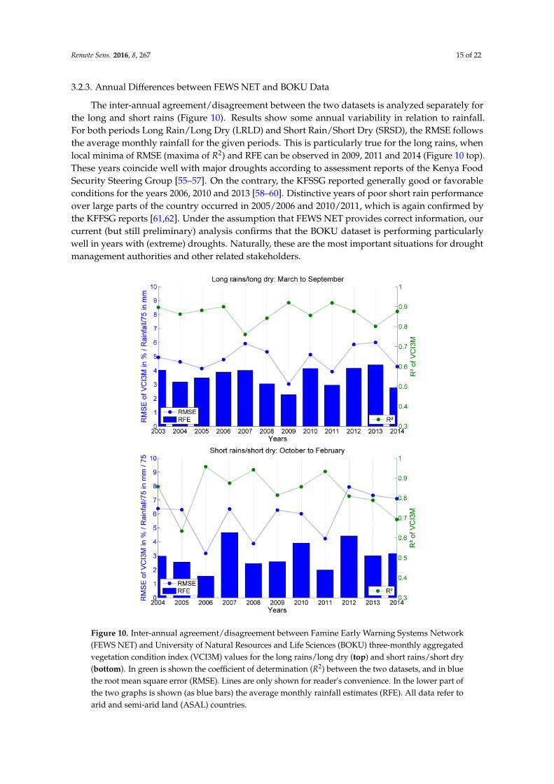
Despite the generally good agreement between the two VCI datasets, somehow larger differencesappear if the analysis is repeated for each month separately. The resulting intra-annual coefficientof determination (R2) varies between 0.77 (November) and 0.94 (February) (Figure 9—green line).Two minima of R2 (and maxima of RMSE) are visible in April and November agreeing very well withKenya’s long and short rains that normally occur in March–June and October–December (blue barsin Figure 9). The largest differences in the VCI3M anomalies occur at the peak of the long and shortrains and in parallel to significant NDVI changes. As cloudiness is the highest during these periods,we expect part of the observed differences stemming from the unfavorable observation conditions.

Remote Sens. 2016, 8, 267 14 of 22Remote Sens. 2016, 8, 267 14 of 22

Figure 8. Correspondence between Famine Early Warning Systems Network (FEWS NET) and University of Natural Resources and Life Sciences (BOKU) datasets of arid and semi-arid land (ASAL) counties across all months between 2003 and 2014 (n = 3312). (left) Scatterplot of three-monthly aggregated vegetation condition index (VCI3M) derived from FEWS NET and BOKU datasets. Also shown the 1-to-1 line (red) and regression line (black); (right) Difference between VCI3M from FEWS NET and BOKU shown as cumulative distribution function.

3.2.2. Seasonal Differences between BOKU and FEWS NET Data

Despite the generally good agreement between the two VCI datasets, somehow larger differences appear if the analysis is repeated for each month separately. The resulting intra-annual coefficient of determination (R2) varies between 0.77 (November) and 0.94 (February) (Figure 9—green line). Two minima of R2 (and maxima of RMSE) are visible in April and November agreeing very well with Kenya’s long and short rains that normally occur in March–June and October–December (blue bars in Figure 9). The largest differences in the VCI3M anomalies occur at the peak of the long and short rains and in parallel to significant NDVI changes. As cloudiness is the highest during these periods, we expect part of the observed differences stemming from the unfavorable observation conditions.

Figure 9. Monthly agreement/disagreement between Famine Early Warning Systems Network (FEWS NET) and University of Natural Resources and Life Sciences (BOKU) three-monthly aggregated vegetation condition index (VCI3M) values. In green is shown the coefficient of determination (R2)

Figure 8. Correspondence between Famine Early Warning Systems Network (FEWS NET) andUniversity of Natural Resources and Life Sciences (BOKU) datasets of arid and semi-arid land (ASAL)counties across all months between 2003 and 2014 (n = 3312). (left) Scatterplot of three-monthlyaggregated vegetation condition index (VCI3M) derived from FEWS NET and BOKU datasets.Also shown the 1-to-1 line (red) and regression line (black); (right) Difference between VCI3M fromFEWS NET and BOKU shown as cumulative distribution function.

Figure 9. Monthly agreement/disagreement between Famine Early Warning Systems Network (FEWSNET) and University of Natural Resources and Life Sciences (BOKU) three-monthly aggregatedvegetation condition index (VCI3M) values. In green is shown the coefficient of determination (R2)between the two datasets, and in blue the root mean square error (RMSE). Lines are only shownfor reader’s convenience. The lower part of the figure shows the climatology of NDVI (orange) andmonthly rainfall estimates (RFE). All data refer to arid and semi-arid land (ASAL) countries.

Remote Sens. 2016, 8, 267 15 of 22

3.2.3. Annual Differences between FEWS NET and BOKU Data

The inter-annual agreement/disagreement between the two datasets is analyzed separately forthe long and short rains (Figure 10). Results show some annual variability in relation to rainfall.For both periods Long Rain/Long Dry (LRLD) and Short Rain/Short Dry (SRSD), the RMSE followsthe average monthly rainfall for the given periods. This is particularly true for the long rains, whenlocal minima of RMSE (maxima of R2) and RFE can be observed in 2009, 2011 and 2014 (Figure 10 top).These years coincide well with major droughts according to assessment reports of the Kenya FoodSecurity Steering Group [55–57]. On the contrary, the KFSSG reported generally good or favorableconditions for the years 2006, 2010 and 2013 [58–60]. Distinctive years of poor short rain performanceover large parts of the country occurred in 2005/2006 and 2010/2011, which is again confirmed bythe KFFSG reports [61,62]. Under the assumption that FEWS NET provides correct information, ourcurrent (but still preliminary) analysis confirms that the BOKU dataset is performing particularlywell in years with (extreme) droughts. Naturally, these are the most important situations for droughtmanagement authorities and other related stakeholders.

Figure 10. Inter-annual agreement/disagreement between Famine Early Warning Systems Network(FEWS NET) and University of Natural Resources and Life Sciences (BOKU) three-monthly aggregatedvegetation condition index (VCI3M) values for the long rains/long dry (top) and short rains/short dry(bottom). In green is shown the coefficient of determination (R2) between the two datasets, and in bluethe root mean square error (RMSE). Lines are only shown for reader's convenience. In the lower part ofthe two graphs is shown (as blue bars) the average monthly rainfall estimates (RFE). All data refer toarid and semi-arid land (ASAL) countries.

Remote Sens. 2016, 8, 267 16 of 22

3.2.4. Spatial Patterns of Agreement/Disagreement between FEWS NET and BOKU Data

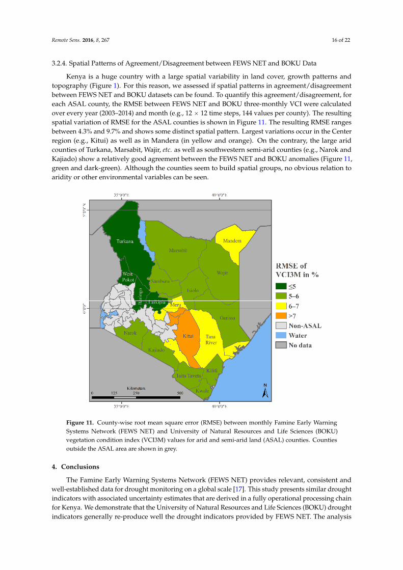
Kenya is a huge country with a large spatial variability in land cover, growth patterns andtopography (Figure 1). For this reason, we assessed if spatial patterns in agreement/disagreementbetween FEWS NET and BOKU datasets can be found. To quantify this agreement/disagreement, foreach ASAL county, the RMSE between FEWS NET and BOKU three-monthly VCI were calculatedover every year (2003–2014) and month (e.g., 12 ˆ 12 time steps, 144 values per county). The resultingspatial variation of RMSE for the ASAL counties is shown in Figure 11. The resulting RMSE rangesbetween 4.3% and 9.7% and shows some distinct spatial pattern. Largest variations occur in the Centerregion (e.g., Kitui) as well as in Mandera (in yellow and orange). On the contrary, the large aridcounties of Turkana, Marsabit, Wajir, etc. as well as southwestern semi-arid counties (e.g., Narok andKajiado) show a relatively good agreement between the FEWS NET and BOKU anomalies (Figure 11,green and dark-green). Although the counties seem to build spatial groups, no obvious relation toaridity or other environmental variables can be seen.

Remote Sens. 2016, 8, 267 16 of 22

3.2.4. Spatial Patterns of Agreement/Disagreement between FEWS NET and BOKU Data

Kenya is a huge country with a large spatial variability in land cover, growth patterns and topography (Figure 1). For this reason, we assessed if spatial patterns in agreement/disagreement between FEWS NET and BOKU datasets can be found. To quantify this agreement/disagreement, for each ASAL county, the RMSE between FEWS NET and BOKU three-monthly VCI were calculated over every year (2003–2014) and month (e.g., 12 × 12 time steps, 144 values per county). The resulting spatial variation of RMSE for the ASAL counties is shown in Figure 11. The resulting RMSE ranges between 4.3% and 9.7% and shows some distinct spatial pattern. Largest variations occur in the Center region (e.g., Kitui) as well as in Mandera (in yellow and orange). On the contrary, the large arid counties of Turkana, Marsabit, Wajir, etc. as well as southwestern semi-arid counties (e.g., Narok and Kajiado) show a relatively good agreement between the FEWS NET and BOKU anomalies (Figure 11, green and dark-green). Although the counties seem to build spatial groups, no obvious relation to aridity or other environmental variables can be seen.

Figure 11. County-wise root mean square error (RMSE) between monthly Famine Early Warning Systems Network (FEWS NET) and University of Natural Resources and Life Sciences (BOKU) vegetation condition index (VCI3M) values for arid and semi-arid land (ASAL) counties. Counties outside the ASAL area are shown in grey.

4. Conclusions

The Famine Early Warning Systems Network (FEWS NET) provides relevant, consistent and well-established data for drought monitoring on a global scale [17]. This study presents similar drought indicators with associated uncertainty estimates that are derived in a fully operational processing chain for Kenya. We demonstrate that the University of Natural Resources and Life Sciences (BOKU) drought indicators generally re-produce well the drought indicators provided by FEWS NET. The analysis shows an overall good agreement with a coefficient of determination (R2) of 0.89 and a root mean square error (RMSE) in the order of 6% for the investigated 3-monthly VCI.

Figure 11. County-wise root mean square error (RMSE) between monthly Famine Early WarningSystems Network (FEWS NET) and University of Natural Resources and Life Sciences (BOKU)vegetation condition index (VCI3M) values for arid and semi-arid land (ASAL) counties. Countiesoutside the ASAL area are shown in grey.

4. Conclusions

The Famine Early Warning Systems Network (FEWS NET) provides relevant, consistent andwell-established data for drought monitoring on a global scale [17]. This study presents similar droughtindicators with associated uncertainty estimates that are derived in a fully operational processing chainfor Kenya. We demonstrate that the University of Natural Resources and Life Sciences (BOKU) droughtindicators generally re-produce well the drought indicators provided by FEWS NET. The analysis

Remote Sens. 2016, 8, 267 17 of 22

shows an overall good agreement with a coefficient of determination (R2) of 0.89 and a root meansquare error (RMSE) in the order of 6% for the investigated 3-monthly VCI. The main advantage of ourdata is that the drought information is provided in near real-time (NRT), without time lag. Positively,the most relevant (driest) years correspond best, e.g., R2 of 0.92 and RMSE of 3%. The highest differenceis a RMSE of 8% and a R2 of 0.63. Intra-annual coefficients of determination between both datasetsdisplay the same order of variations with a R2 of 0.77 for November and 0.94 for February.

The BOKU data presented in this paper are delivered to NDMA within 2–3 days after the lastMonday in a given month. For comparison, the consolidated FEWS NET data are only availablefive to six weeks after the end of each month. This offers an improved timeliness for deploymentof disaster contingency funds (DCF) and other (financial and humanitarian) interventions. Kenya’sNational Drought Monitoring Authority (NDMA) uses for example our timely data for triggering theDCF payments. In a very similar way, the Hunger Safety Net Program (HSNP) of Kenya uses BOKUindicators for cash transfers to households in need.

Despite the overall good agreement between FEWS NET and our indicators, we observe somepersistent (seasonal and spatial) differences between the two datasets. These differences deservefurther research—not only from a scientific point of view, but also because such differences mightconfuse stakeholders, and therefore erode the trust in the remotely sensed information. We planto improve our NRT processing by incorporating for example daily or eight-day MOD09 products(collection 6) into the filtering process, as well as additional data sources such as Proba-V.

For the analysis provided in this paper, it has to be highlighted that the FEWS NET data weretaken as “reference” to which the BOKU data were compared. Future research should comparethe two datasets against an external reference. Ideally, such an external reference would consist ofmulti-year in-situ biomass measurements. We do not recommend using rainfall measurements asreference information as they only capture meteorological drought; the impact on grazing conditionsand agriculture remains unknown. In addition, spatially explicit rainfall estimates from satelliteobservations have their own limitations and uncertainties.

Acknowledgments: Research described in this contribution was partly financed through EC’s funding undera service contract provided by NDMA. We thank Luigi Luminari and James Oduor (both NDMA, Nairobi)for having made this possible. The MODIS MOD13Q1, MYD13Q1 and MCD12Q1 data processed in BOKU’sNRT processing chain were obtained through the online Data Pool at the NASA Land Processes DistributedActive Archive Center (LP DAAC), USGS/Earth Resources Observation and Science (EROS) Center, Sioux Falls,South Dakota (https://lpdaac.usgs.gov/get_data). The eMODIS NDVI data were obtained through the FamineEarly Warning Systems Network (FEWS NET) data portal provided by the USGS FEWS NET Project, part ofthe Early Warning and Environmental Monitoring Program at the USGS Earth Resources Observation andScience (EROS) Center. This is acknowledged. We further acknowledge the support of Matteo Mattiuzzifor R code development as well as Francesco Vuolo and Martin Siklar (all from BOKU) for setting upthe two web-tools for data display (http://ivfl-geomap.boku.ac.at/demo_WG/kenya/) and data analysis(http://ivfl-info.boku.ac.at/index.php/eo-data-processing/data-analytics). We thank Valentin Pesendorfer(BOKU) for his help in producing the land cover map of Kenya. We also acknowledge the fact that part ofthe computations has been done using the Vienna Scientific Cluster (VSC). We are very grateful to the Universityof Reading, and Elena Tarnavsky for providing access to TAMSAT rainfall data. We thank JRC and Felix Remboldfor access to SPIRITS software.

Author Contributions: Anja Klisch and Clement Atzberger contributed equally to this manuscript.

Conflicts of Interest: The authors declare no conflict of interest.

Appendix

Web Interfaces

The operational drought-related information products (Table 3—upper part) are delivered toNDMA at the end of each month via FTP server. This includes image files (e.g., GeoTiff and genericbinaries), but also KMZ files and quick looks (QLK), as well as spatially aggregated drought indicatorsfor producing charts and figures using the SPIRITS software [50]. Part of the data can also be accessedonline (see Table 3). Exemplary figures of the online possibilities are shown in Figures A1 and A2 [51].

Remote Sens. 2016, 8, 267 18 of 22

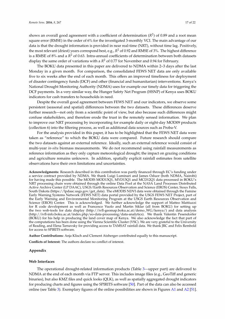
Figure A1 contains the web interface for displaying the spatially aggregated drought indicatorsfor the example of the three-monthly VCI (June 2015) at sub-county level in Kenya. Only sub-countiesclassified as “pastoralist” are displayed (all other counties in grey). Pixels not classified as “pastoralist”are excluded from the aggregated statistics. Statistics are derived by averaging the pixel-wise VCIvalues. Details for the Samburu East County (Figure A1 left side) are also shown. This informationcan be obtained by clicking on the sub-county in the map (here located in the center of Kenya—blackborder). The top graph shows information about RFE (in blue bars, long-term average and actual data)as well as for three-monthly VCI (actual year in purple, historical minimum in red, historical maximumin green and historical median in yellow). The below matrix plot is the classified three-monthly VCI(color coding according to Table 4—missing data in grey).

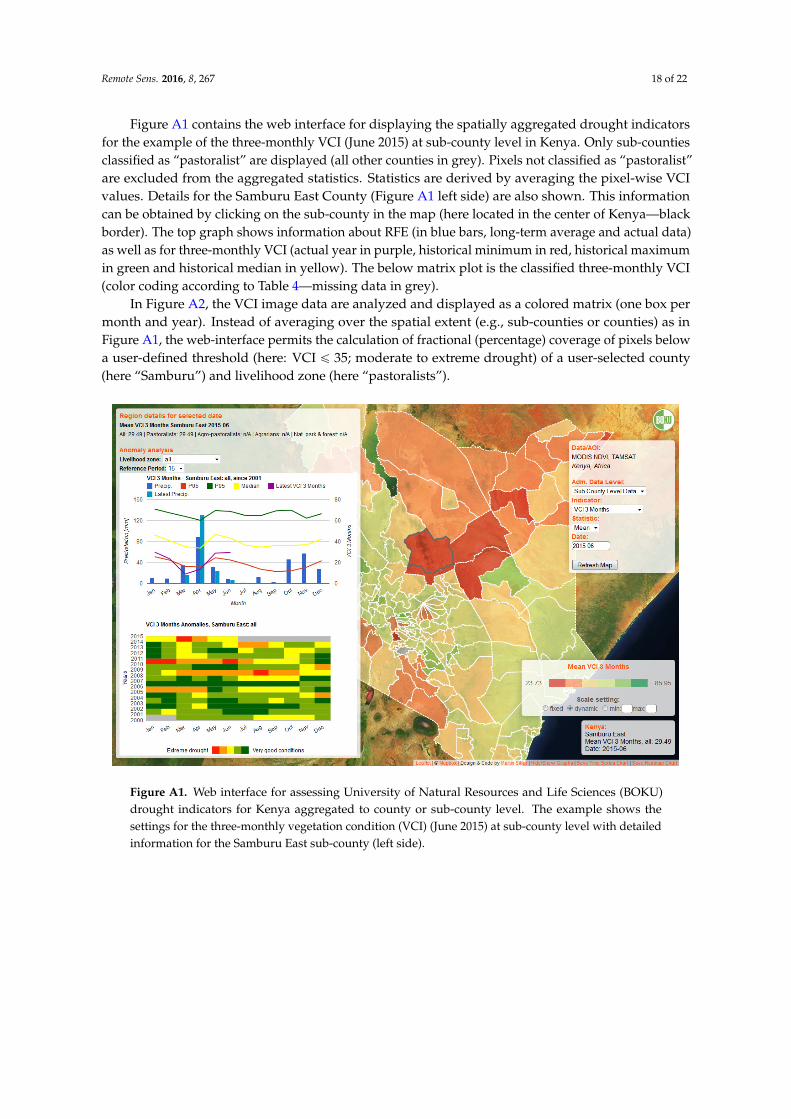
In Figure A2, the VCI image data are analyzed and displayed as a colored matrix (one box permonth and year). Instead of averaging over the spatial extent (e.g., sub-counties or counties) as inFigure A1, the web-interface permits the calculation of fractional (percentage) coverage of pixels belowa user-defined threshold (here: VCI ď 35; moderate to extreme drought) of a user-selected county(here “Samburu”) and livelihood zone (here “pastoralists”).

Remote Sens. 2016, 8, 267 18 of 22

Figure A1 contains the web interface for displaying the spatially aggregated drought indicators for the example of the three-monthly VCI (June 2015) at sub-county level in Kenya. Only sub-counties classified as “pastoralist” are displayed (all other counties in grey). Pixels not classified as “pastoralist” are excluded from the aggregated statistics. Statistics are derived by averaging the pixel-wise VCI values. Details for the Samburu East County (Figure A1 left side) are also shown. This information can be obtained by clicking on the sub-county in the map (here located in the center of Kenya—black border). The top graph shows information about RFE (in blue bars, long-term average and actual data) as well as for three-monthly VCI (actual year in purple, historical minimum in red, historical maximum in green and historical median in yellow). The below matrix plot is the classified three-monthly VCI (color coding according to Table 4—missing data in grey).

In Figure A2, the VCI image data are analyzed and displayed as a colored matrix (one box per month and year). Instead of averaging over the spatial extent (e.g., sub-counties or counties) as in Figure A1, the web-interface permits the calculation of fractional (percentage) coverage of pixels below a user-defined threshold (here: VCI ≤ 35; moderate to extreme drought) of a user-selected county (here “Samburu”) and livelihood zone (here “pastoralists”).

Figure A1. Web interface for assessing University of Natural Resources and Life Sciences (BOKU) drought indicators for Kenya aggregated to county or sub-county level. The example shows the settings for the three-monthly vegetation condition (VCI) (June 2015) at sub-county level with detailed information for the Samburu East sub-county (left side).

Figure A1. Web interface for assessing University of Natural Resources and Life Sciences (BOKU)drought indicators for Kenya aggregated to county or sub-county level. The example shows thesettings for the three-monthly vegetation condition (VCI) (June 2015) at sub-county level with detailedinformation for the Samburu East sub-county (left side).

Remote Sens. 2016, 8, 267 19 of 22Remote Sens. 2016, 8, 267 19 of 22

Figure A2. Web interface for assessing University of Natural Resources and Life Sciences (BOKU) drought indicators for Kenya aggregated to county level. In the example, an area is shown (percentage of Samburu county) where the vegetation condition index (VCI) is below 35 (moderate to extreme drought).

References

1. Heim, R.R., Jr. A review of twentieth-century drought indices used in the United States. B Am. Meteorol. Soc. 2002, 83, 1149–1165.

2. Anderson, W.B.; Zaitchik, B.F.; Hain, C.R.; Anderson, M.C.; Yilmaz, M.T.; Mecikalski, J.; Schultz, L. Towards an integrated soil moisture drought monitor for East Africa. Hydrol. Earth. Syst. Sci. 2012, 16, 2893–2913.

3. Wilhite, D.; Buchanan-Smith, M. Drought as a natural hazard: Understanding the natural and social context. In Drought and Water Crises: Science, Technology, and Management Issues; Wilhite, D., Ed.; CRC Press: Boca Raton, FL, USA, 2005; pp. 3–29.

4. Below, R.; Grover-Kopec, E.; Dilley, M. Documenting drought-related disasters: A global reassessment. J. Environ. Dev. 2007, 16, 328–344.

5. Vicente-Serrano, S.M.; Beguería, S.; Gimeno, L.; Eklundh, L.; Giuliani, G.; Weston, D.; Kenawy, A.E.; López-Moreno, J.I.; Nieto, R.; Ayenew, T.; et al. Challenges for drought mitigation in Africa: The potential use of geospatial data and drought information systems. Appl. Geogr. 2012, 34, 471–486.

6. Mishra, A.K.; Singh, V.P. A review of drought concepts. J. Hydrol. 2010, 391, 202–216. 7. Brown, M.; Funk, C.; Galu, U.; Choularton, R. Earlier famine warning possible using remote sensing and

models. EOS 2007, 88, 381–398. 8. Brown, M. Famine Early Warning Systems and Remote Sensing Data; Springer: Oakton, IL, USA, 2008. 9. Vrieling, A.; Meroni, M.; Shee, A.; Mude, A.G.; Woodard, J.; de Bie, C.K.; Rembold, F. Historical extension

of operational NDVI products for livestock insurance in Kenya. Int. J. Appl. Earth Obs. Geoinf. 2014, 28, 238–251.

Figure A2. Web interface for assessing University of Natural Resources and Life Sciences (BOKU)drought indicators for Kenya aggregated to county level. In the example, an area is shown(percentage of Samburu county) where the vegetation condition index (VCI) is below 35 (moderate toextreme drought).

References

1. Heim, R.R., Jr. A review of twentieth-century drought indices used in the United States. B Am. Meteorol. Soc.2002, 83, 1149–1165.

2. Anderson, W.B.; Zaitchik, B.F.; Hain, C.R.; Anderson, M.C.; Yilmaz, M.T.; Mecikalski, J.; Schultz, L. Towardsan integrated soil moisture drought monitor for East Africa. Hydrol. Earth. Syst. Sci. 2012, 16, 2893–2913.[CrossRef]

3. Wilhite, D.; Buchanan-Smith, M. Drought as a natural hazard: Understanding the natural and socialcontext. In Drought and Water Crises: Science, Technology, and Management Issues; Wilhite, D., Ed.; CRC Press:Boca Raton, FL, USA, 2005; pp. 3–29.

4. Below, R.; Grover-Kopec, E.; Dilley, M. Documenting drought-related disasters: A global reassessment.J. Environ. Dev. 2007, 16, 328–344. [CrossRef]

5. Vicente-Serrano, S.M.; Beguería, S.; Gimeno, L.; Eklundh, L.; Giuliani, G.; Weston, D.; Kenawy, A.E.;López-Moreno, J.I.; Nieto, R.; Ayenew, T.; et al. Challenges for drought mitigation in Africa: The potentialuse of geospatial data and drought information systems. Appl. Geogr. 2012, 34, 471–486. [CrossRef]

6. Mishra, A.K.; Singh, V.P. A review of drought concepts. J. Hydrol. 2010, 391, 202–216. [CrossRef]7. Brown, M.; Funk, C.; Galu, U.; Choularton, R. Earlier famine warning possible using remote sensing and

models. EOS 2007, 88, 381–398. [CrossRef]8. Brown, M. Famine Early Warning Systems and Remote Sensing Data; Springer: Oakton, IL, USA, 2008.

Remote Sens. 2016, 8, 267 20 of 22

9. Vrieling, A.; Meroni, M.; Shee, A.; Mude, A.G.; Woodard, J.; de Bie, C.K.; Rembold, F. Historical extension ofoperational NDVI products for livestock insurance in Kenya. Int. J. Appl. Earth Obs. Geoinf. 2014, 28, 238–251.[CrossRef]

10. Rembold, F.; Atzberger, C.; Savin, I.; Rojas, O. Using low resolution satellite imagery for yield prediction andyield anomaly detection. Remote Sens. 2013, 5, 1704–1733. [CrossRef]

11. Thenkabail, P.S. Remote Sensing of Water Resources, Disasters, and Urban Studies; CRC Press: Boca Raton, FL,USA, 2015.

12. Kogan, F.; Guo, W. Agricultural drought detection and monitoring using vegetation health methods.In Remote Sensing of Water Resources, Disasters, and Urban Studies; Thenkabail, P.S., Ed.; CRC Press: Boca Raton,FL, USA, 2015; pp. 339–348.

13. Rembold, F.; Meroni, M.; Rojas, O.; Atzberger, C.; Ham, F.; Fillol, E. Agricultural drought monitoring usingspace-derived vegetation and biophysical products. In Remote Sensing of Water Resources, Disasters, and UrbanStudies; Thenkabail, P.S., Ed.; CRC Press: Boca Raton, FL, USA, 2015; pp. 349–366.

14. Wardlow, B.; Anderson, M.; Tadesse, T.; Hain, C.; Crow, W.; Rodell, M. Remote sensing of drought: Emergenceof a satellite-based monitoring toolkit for the United States. In Remote Sensing of Water Resources, Disasters,and Urban Studies; Thenkabail, P.S., Ed.; CRC Press: Boca Raton, FL, USA, 2015; pp. 367–400.

15. Rhee, J.; Im, J.; Park, S. Regional drought monitoring based on multisensor remote sensing. In Remote Sensingof Water Resources, Disasters, and Urban Studies; Thenkabail, P.S., Ed.; CRC Press: Boca Raton, FL, USA, 2015;pp. 401–416.

16. Senay, G.; Velpuri, N.; Bohms, S.; Budde, M.; Young, C.; Rowland, J.; Verdin, J. Drought monitoring andassessment: Remote sensing and modeling approaches for the Famine Early Warning Systems Network.In Hydro-Meteorological Hazards, Risks and Disasters; Paron, P., Di Baldassarre, G., Shroder, J.F., Eds.; Elsevier:Boston, MA, USA, 2015; pp. 233–262.

17. Svoboda, M. An introduction to the drought monitor. Drought Network News 2000, 12, 80.18. Sivakumar, M., Motha, R., Wilhite, D., Qu, J., Eds.; Towards a compendium on national drought policy.

In Proceedings of the Expert Meeting on the Preparation of a Compendium on National Drought Policy,Washington, DC, USA, 14–15 July 2011; World Meteorological Organization: Geneva, Switzerland, 2011.

19. Vrieling, A.; Meroni, M.; Mude, A.; Chantarat, S.; Ummenhofer, C.; de Bie, K. Early assessment of seasonalforage availability for mitigating the impact of drought on East African pastoralists. Remote Sens. Environ.2016, 174, 44–55. [CrossRef]

20. Tadesse, T.; Haile, M.; Senay, G.; Wardlow, B.D.; Knutson, C.L. The need for integration of drought monitoringtools for proactive food security management in sub-Saharan Africa. Nat. Resour. Forum 2008, 32, 265–279.[CrossRef]

21. Tadesse, T.; Wardlow, B.D.; Hayes, M.J.; Svoboda, M.D.; Brown, J.F. The vegetation outlook (VegOut): A newmethod for predicting vegetation seasonal greenness. GISci. Remote Sens. 2010, 47, 25–52. [CrossRef]

22. Sheffield, J.; Wood, E.F.; Chaney, N.; Guan, K.; Sadri, S.; Yuan, X.; Olang, L.; Amani, A.; Ali, A.; Demuth, S.;et al. A drought monitoring and forecasting system for sub-Sahara African water resources and food security.Bull. Am. Meteor. Soc. 2014, 95, 861–882. [CrossRef]

23. Rojas, O.; Vrieling, A.; Rembold, F. Assessing drought probability for agricultural areas in Africa with coarseresolution remote sensing imagery. Remote Sens. Environ. 2011, 115, 343–352. [CrossRef]

24. Hird, J.; McDermid, G. Noise reduction of NDVI time series: An empirical comparison of selected techniques.Remote Sens. Environ. 2009, 113, 248–258. [CrossRef]

25. Atzberger, C.; Eilers, P.H.C. Evaluating the effectiveness of smoothing algorithms in the absence of groundreference measurements. Int. J. Remote Sens. 2011, 32, 3689–3709. [CrossRef]

26. Atkinson, P.M.; Jeganathan, C.; Dash, J.; Atzberger, C. Intercomparison of four models for smoothingsatellite sensor time-series data to estimate vegetation phenology. Remote Sens. Environ. 2012, 123, 400–417.[CrossRef]

27. Geng, L.; Ma, M.; Wang, X.; Yu, W.; Jia, S.; Wang, H. Comparison of eight techniques for reconstructingmulti-satellite sensor time-series NDVI data sets in the Heihe River basin, China. Remote Sens. 2014, 6,2024–2049. [CrossRef]

28. Kandasamy, S.; Fernandes, R. An approach for evaluating the impact of gaps and measurement errorson satellite land surface phenology algorithms: Application to 20 year NOAA AVHRR data over Canada.Remote Sens. Environ. 2015, 164, 114–129. [CrossRef]

Remote Sens. 2016, 8, 267 21 of 22

29. Shao, Y.; Lunetta, R.S.; Wheeler, B.; Iiames, J.S.; Campbell, J.B. An evaluation of time-series smoothingalgorithms for land-cover classifications using MODIS-NDVI multi-temporal data. Remote Sens. Environ.2016, 174, 258–265. [CrossRef]

30. Eilers, P.H.C. A perfect smoother. Anal. Chem. 2003, 75, 3631–3636. [CrossRef] [PubMed]31. Eilers, P.H.C.; Marx, B.D. Splines, knots, and penalties. Wiley Interdiscip. Rev. Comput. Stat. 2010, 2, 637–653.

[CrossRef]32. Atzberger, C.; Eilers, P.H.C. A time series for monitoring vegetation activity and phenology at 10-daily time

steps covering large parts of South America. Int. J. Digit. Earth 2011, 4, 365–386. [CrossRef]33. Atzberger, C.; Klisch, A.; Mattiuzzi, M.; Vuolo, F. Phenological metrics derived over the European continent

from NDVI3g data and MODIS time series. Remote Sens. 2014, 6, 257–284. [CrossRef]34. Maidment, R.I.; Grimes, D.; Allan, R.P.; Tarnavsky, E.; Stringer, M.; Hewison, T.; Roebeling, R.; Black, E.

The 30 years TAMSAT African rainfall climatology and time series (TARCAT) data set. J. Geophys. Res. A2014, 119, 10619–10644. [CrossRef]

35. Tarnavsky, E.; Grimes, D.; Maidment, R.; Black, E.; Allan, R.P.; Stringer, M. Extension of the TAMSATsatellite-based rainfall monitoring over Africa and from 1983 to present. J. Appl. Meteorol. 2014, 53, 2805–2822.[CrossRef]

36. Brown, M. Biophysical remote sensing and climate data in famine early warning systems. Geogr. Compass2009, 3, 1381–1407. [CrossRef]

37. Meroni, M.; Verstraete, M.M.; Rembold, F.; Urbano, F.; Kayitakire, F. A phenology-based method to derivebiomass production anomalies for food security monitoring in the Horn of Africa. Int. J. Remote Sens. 2014,35, 2472–2492. [CrossRef]

38. Kenya GIS Data. World Resources Institute (WRI). Available online: http://www.wri.org/resources/data-sets/kenya-gis-data (accessed on 26 February 2016).

39. TAMSAT (Tropical Applications of Meteorology Using SATellite Data and Ground-Based Observations).University of Reading. Available online: http://www.met.reading.ac.uk/~tamsat/data/ (accessed on26 February 2016).

40. Solano, R.; Didan, K.; Jacobson, A.; Huete, A. MODIS Vegetation Index User’s Guide (MOD13 Series),Version 2.00, May 2010 (Collection 5). Vegetation Index and Phenology Lab, The University of Arizona. 2010.Available online: http://www.ctahr.hawaii.edu/grem/modis-ug.pdf (accessed on 9 March 2016).

41. Mattiuzzi, M.; Verbesselt, J.; Hengl, T.; Klisch, A.; Evans, B.; Lobo, A. MODIS: MODIS download andprocessing package. In Processing Functionalities for (Multi-Temporal) MODIS Grid Data. First InternationalWorkshop on “Temporal Analysis of Satellite Images”, Mykonos Island, Greece, 23–25 May 2012.

42. Vuolo, F.; Atzberger, C. Exploiting the classification performance of support vector machines withmulti-temporal Moderate-Resolution Imaging Spectroradiometer (MODIS) data in areas of agreementand disagreement of existing land cover products. Remote Sens. 2012, 4, 3143–3167. [CrossRef]

43. Sedano, F.; Kempeneers, P.; Hurtt, G. A Kalman filter-based method to generate continuous time series ofmedium-resolution NDVI images. Remote Sens. 2014, 6, 12381–12408. [CrossRef]

44. Beck, P.S.A.; Atzberger, C.; Høgda, K.A.; Johansen, B.; Skidmore, A.K. Improved monitoring of vegetationdynamics at very high latitudes: A new method using MODIS NDVI. Remote Sens. Environ. 2006, 100,321–334. [CrossRef]

45. Brown, M.; Lary, D.; Vrieling, A.; Stathakis, D.; Mussa, H. Neural networks as a tool for constructingcontinuous NDVI time series from AVHRR and MODIS. Int. J. Remote Sens. 2008, 29, 7141–7158. [CrossRef]

46. Bradley, B.; Jacob, R.; Hermance, W. A curve fitting procedure to derive inter-annual phenologies from timeseries of noisy satellite NDVI data. Remote Sens. Environ. 2007, 106, 137–145. [CrossRef]

47. Chen, J.; Jönsson, P.; Tamura, M.; Gu, Z. A simple method for reconstructing a high-quality NDVI time-seriesdata set based on the Savitzky–Golay filter. Remote Sens. Environ. 2004, 91, 332–344. [CrossRef]

48. Viovy, N.; Arino, O.; Belward, A. The Best Index Slope Extraction (BISE): A method for reducing noise inNDVI time-series. Int. J. Remote Sens. 1992, 13, 1585–1590. [CrossRef]

49. Kogan, F.; Gitelson, A.; Zakarin, E.; Spivak, L.; Lebed, L. AVHRR-based spectral vegetation index forquantitative assessment of vegetation state and productivity: Calibration and validation. Photogramm. Eng.Remote Sens. 2003, 69, 809–906. [CrossRef]

Remote Sens. 2016, 8, 267 22 of 22

50. Rembold, F.; Meroni, M.; Urbano, F.; Royer, A.; Atzberger, C.; Lemoine, G.; Eerens, H.; Haesen, D. Remotesensing time series analysis for crop monitoring with the SPIRITS software: New functionalities and useexamples. Front. Environ. Sci. 2015, 3. [CrossRef]

51. Web-tools for Vegetation Anomaly Analysis. BOKU. Available online: http://ivfl-geomap.boku.ac.at/demo_WG/kenya/, http://ivfl-info.boku.ac.at/index.php/eo-data-processing/data-analytics (accessed on26 February 2016).

52. USGS. eMODIS Africa Product Guide Version 1.0, 2011; USGS EROS Data Center: Sioux Falls, SD, USA, 2011.53. USGS. eMODIS TERRA Normalized Difference Vegetation Index (NDVI). 2013. Available online:

http://earlywarning.usgs.gov/fews/product/116 (accessed on 16 March 2016).54. Colditz, R.R.; Conrad, C.; Wehrmann, T.; Schmidt, M.; Dech, S. Analysis of the quality of collection 4 and 5

vegetation index time series from MODIS. In Proceedings of the ISPRS 5th International Symposium SpatialData Quality, Enschede, The Netherlands, 13–15 June 2007; Volume XXXVI-2/C43.

55. KFSSG. Kenya Long Rains Assessment Report 2009. Technical Report, Kenya Food SecuritySteering Group (KFSSG). 2009. Available online: http://documents.wfp.org/stellent/groups/public/documents/ena/wfp208056.pdf?iframe (accessed on 9 March 2016).

56. KFSSG. Kenya Long Rains Assessment Report 2011. Technical Report, Kenya Food Security SteeringGroup (KFSSG). 2011. Available online: http://documents.wfp.org/stellent/groups/public/documents/ena/wfp240180.pdf (accessed on 9 March 2016).

57. KFSSG. Kenya Long Rains Assessment Report 2014. Technical Report, Kenya Food Security SteeringGroup (KFSSG). 2014. Available online: http://www.ipcinfo.org/fileadmin/user_upload/ipcinfo/docs/2014%20Kenya%20LRA%20National%20Report.pdf (accessed on 9 March 2016).

58. KFSSG. Kenya Long Rains Assessment Report 2006. Technical Report, Kenya Food Security SteeringGroup (KFSSG). 2006. Available online: http://reliefweb.int/sites/reliefweb.int/files/resources/F63B1A92E605B2E4C1257230004B666F-govt-ken-12sep.pdf (accessed on 9 March 2016).

59. KFSSG. Kenya Long Rains Assessment Report 2010. Technical Report, Kenya Food Security SteeringGroup (KFSSG). 2010. Available online: http://www.fao.org/fileadmin/user_upload/drought/docs/Kenya_2010_LRA%20Report.pdf (accessed on 9 March 2016).

60. KFSSG. Kenya Long Rains Assessment Report 2013. Technical Report, Kenya Food Security SteeringGroup (KFSSG). 2013. Available online: https://www.humanitarianresponse.info/system/files/documents/files/LRA%202013_National%20Report_Final.pdf (accessed on 9 March 2016).

61. KFSSG. Kenya Short Rains Assessment Report 2005. Technical Report, Kenya Food Security SteeringGroup (KFSSG). 2006. Available online: http://documents.wfp.org/stellent/groups/public/documents/ena/wfp087348.pdf?iframe (accessed on 9 March 2016).

62. KFSSG. Kenya Short Rains Assessment Report 2010. Technical Report, Kenya Food Security SteeringGroup (KFSSG). 2011. Available online: http://documents.wfp.org/stellent/groups/public/documents/ena/wfp241326.pdf?iframe (accessed on 9 March 2016).

© 2016 by the authors; licensee MDPI, Basel, Switzerland. This article is an open accessarticle distributed under the terms and conditions of the Creative Commons by Attribution(CC-BY) license (http://creativecommons.org/licenses/by/4.0/).