Operation Manual - GEO SUSTAVI · SOUTH SURVEYING &MAPPING INSTRUMENT ... Thank you for purchasing...
214
Transcript of Operation Manual - GEO SUSTAVI · SOUTH SURVEYING &MAPPING INSTRUMENT ... Thank you for purchasing...


Operation Manual
NTS-960R Series Electronic Total Station
SOUTH SURVEYING &MAPPING INSTRUMENT CO., LTD

INDEX
FOREWORD .............................................................................................................................................. 1
PRECAUTIONS ......................................................................................................................................... 2
SAFETY GUIDE ........................................................................................................................................ 3
1. NOMENCLATURE AND FUNCTIONS .............................................................................................. 4
1.1 NOMENCLATURE ............................................................................................................................ 4 1.2 KEYPAD ............................................................................................................................................ 6
2. SYNCHRONIZATION WITH PC ........................................................................................................ 7
2.1 INSTALLATION MICROSOFT ACTIVESYNC ............................................................................... 7 2.2 CONNECTING TOTAL STATION WITH PC ................................................................................... 7
3. KNOWING ABOUT WINCE(R) .......................................................................................................... 9
3.1 OPERATING SYSTEM ...................................................................................................................... 9 3.2 SETTING YOUR TOTAL STATION ................................................................................................. 9
3.2.1 Backlight ..................................................................................................................................... 9 3.2.2 Touch-screen Adjustment .......................................................................................................... 11
3.3 APPROACHES TO INPUT NUMERAL AND CHARACTER ........................................................ 12
4.STAR KEY (★) MODE ..................................................................................................................... 16
5. PREPARATION FOR MEASUREMENT ......................................................................................... 18
5.1 UNPACKING AND STORE OF INSTRUMENT ............................................................................ 18 5.2 INSTRUMENT SETUP .................................................................................................................... 18 5.3 BATTERY INFORMATION ............................................................................................................ 21 5.4 REFLECTOR PRISM ....................................................................................................................... 22 5.5 MOUNTING AND DISMOUNTING INSTRUMENT FROM TRIBRACH ................................... 22 5.6 EYEPIECE ADJUSTMENT AND COLLIMATING OBJECT ........................................................ 23 5.7 VERTICAL AND HORIZONTAL ANGLE TILT CORRECTION ................................................... 24
6. BASIC SURVEY ................................................................................................................................... 25
6.1 ANGLE MEASUREMENT .............................................................................................................. 26 6.1.1 Horizontal Angle (Right Angle) and Vertical Angle Measurement ........................................... 26 6.1.2 Switch Horizontal Angle Right/Left .......................................................................................... 27 6.1.3 Horizontal Angle Reading Setting ............................................................................................. 28

6.1.4 Vertical Angle Percentage (%) Mode ........................................................................................ 30 6.1.5 Repeat Angle Measurement ....................................................................................................... 31
6.2 DISTANCE MEASUREMENT ........................................................................................................ 33 6.2.1 Setting Atmosphere Correction ................................................................................................. 34 6.2.2 Atmospheric Refraction And Earth Curvature Correction ......................................................... 37 6.2.3 Setting Target Type .................................................................................................................... 38 6.2.4Setting the Prism Constant ......................................................................................................... 39 6.2.5Distance Measurement (Continue Measurement) ...................................................................... 40 6.2.6 Distance Measurement (Single/N-Time Measurement) ............................................................ 41 6.2.7Fine/Tracking Measurement Mode ............................................................................................. 42
6.3 COORDINATE MEASUREMENT .................................................................................................. 43 6.3.1 Setting Coordinate Values of Occupied Point ........................................................................... 43 6.3.2 Setting the Backsight Point ....................................................................................................... 45 6.3.3 Setting the Instrument Height/ Prism Height ............................................................................. 46 6.3.4 Operation of Coordinate Measurement ..................................................................................... 47
7. APPLICATION PROGRAMS ............................................................................................................. 48
7.1 LAYOUT .......................................................................................................................................... 48 7.2 REMOTE ELEVATION MEASUREMENT (REM) ........................................................................ 49
7.2.1 Inputting Prism Height (h) ......................................................................................................... 50 7.2.2 without Inputtingt Prism Height ................................................................................................ 51
7.3 MISSING LINE MEASUREMENT (MLM) .................................................................................... 53 7.4 LINE MEASUREMENT (LINE) ...................................................................................................... 56 7.5 LEAD MEASUREMENT (STORE NEZ) ........................................................................................ 59 7.6 OFFSET MEASUREMENT (OFFSET) ........................................................................................... 62
7.6.1 Angle Offset .............................................................................................................................. 62 7.6.2 Distance Offset .......................................................................................................................... 64 7.6.3 Column Offset ........................................................................................................................... 65 7.6.4 Plane Offset ............................................................................................................................... 67
7.7 PARAMETERS SETTING ............................................................................................................... 69
8. START STANDARD SURVEY PROGRAM ...................................................................................... 71
9. PROJECT ............................................................................................................................................. 74
9.1 CREATE NEW PROJECT ................................................................................................................ 75 9.2 OPEN PROJECT .............................................................................................................................. 76 9.3 DELETE PROJECT .......................................................................................................................... 76 9.4 OPTION ............................................................................................................................................ 78 9.5 GRID FACTOR ................................................................................................................................ 79

10. DATA EXPORT/IMPORT ................................................................................................................. 80
10.1 DATA EXPORT .............................................................................................................................. 80 10.2 DATA IMPORT............................................................................................................................... 82
11. RECORD MEASUREMENT DATA ................................................................................................. 84
11.1 SETTING OCCUPIED POINT AND BACKSIGHT POINT .......................................................... 85 11.2 BACKSIGHT OBSERVATION (BS OBS) ..................................................................................... 96 11.3 FORESIGHT OBSERVATION (FS OBS) ....................................................................................... 97 11.4 SIDESHOT OBSERVATION (SS OBS) ......................................................................................... 99
11.4.1 Offset ..................................................................................................................................... 101 11.4.2 Plane Offset ........................................................................................................................... 104 11.4.3 Pt. Line Mode (For Measurement from Point to Line) .......................................................... 106 11.4.4 Control Input ......................................................................................................................... 108
11.5 CROSS SECTION SURVEY ........................................................................................................ 109
12. EDIT DATA ....................................................................................................................................... 112
12.1 EDITING RAW DATA ................................................................................................................. 113 12.2 COORD. DATA ............................................................................................................................ 115
12.2.1 Edit Coord. Data .................................................................................................................... 115 12.2.2 Add coord. data ...................................................................................................................... 117 12.2.3 Delete Coord. Data ................................................................................................................ 118
12.3 FIXED POINT DATA ................................................................................................................... 119 12.4 CODE DATA ................................................................................................................................ 119
12.4.1 Create New Layer .................................................................................................................. 119 12.4.2 Edit Layer/Code .................................................................................................................... 121 12.4.3Delete Code ............................................................................................................................ 122
12.5 FILL-CUT DATA ......................................................................................................................... 123
13. PROGRAM MENU .......................................................................................................................... 124
13.1 SET OUT ...................................................................................................................................... 124 13.1.1 Occupied Point& Backsight Point ......................................................................................... 124 13.1.2 Point Set Out ......................................................................................................................... 126 13.1.3 String Setout .......................................................................................................................... 130
13.2 ROAD DESIGN AND LAYOUT .................................................................................................. 131 13.2.1 Define Horizontal Alignment ................................................................................................ 131 13.2.2 Edit Alignment ...................................................................................................................... 137 13.2.3 Define Vertical Alignment ..................................................................................................... 139 13.2.4 Edit Vertical Alignment ......................................................................................................... 140 13.2.5 Alignment Setout ................................................................................................................... 142

13.2.6 Slope Setout ........................................................................................................................... 145 13.2.7 Cross Section Setout .............................................................................................................. 148
13.3 COGO ........................................................................................................................................... 150 13.3.1 Intersection ............................................................................................................................ 150 13.3.2 4-Intersection ......................................................................................................................... 151 13.3.3 Inverse ................................................................................................................................... 153 13.3.4 Area ....................................................................................................................................... 154 13.3.5 Missing Line Measurement ................................................................................................... 157 13.3.6 Radiate ................................................................................................................................... 159
13.4 TRAVERSE ADJUSTMENT ........................................................................................................ 160 13.5 BATTER BOARDS ...................................................................................................................... 167
13.5.1 Method 1: Batter board using two sides ................................................................................ 167 13.5.2 Method 2: Batterboards using one side ................................................................................. 170
13.6 TAPE DIMENSIONS ................................................................................................................... 172
14. SYSTEM SETTINGS ....................................................................................................................... 175
14.1 SETTING UNIT AND MEASURING PARAMETER ................................................................. 175 14.2 SETTING ATMOSPHERE DATA AND PRISM CONSTANT ..................................................... 178
15. CHECK AND ADJUSTMENT ........................................................................................................ 180
15.1 PLATE VIAL ................................................................................................................................ 180 15.2 CIRCULAR VIAL ........................................................................................................................ 180 15.3 INCLINATION OF RETICLE ...................................................................................................... 181 15.4 PERPENDICULARITY BETWEEN LINE OF SIGHT AND HORIZONTAL AXIS (2C) .......... 182 15.5 VERTICAL INDEX DIFFERENCE COMPENSATION .............................................................. 184 15.6 ADJUSTMENT OF VERTICAL INDEX DIFFERENCE (I ANGLE) AND SETTING VERTICAL
INDEX 0 ............................................................................................................................................... 185 15.7 TRANSVERSE AXIS ERROR COMPENSATION ADJUSTMENT ........................................... 186 15.8 OPTICAL PLUMMET ................................................................................................................. 188 15.9 INSTRUMENT CONSTANT(K) ............................................................................................ 189 15.10 PARALLEL BETWEEN LINE OF SIGHT AND EMITTING PHOTOELECTRIC AXIS ......... 191 15.11 TRIBRACH LEVELING SCREW ............................................................................................. 191 15.12 RELATED PARTS FOR REFLECTOR ...................................................................................... 191
16. ACCESSORIES ................................................................................................................................ 193
【APPENDIX-A】 ................................................................................................................................. 194
1 EXPORT DATA FROM TOTAL STATION ....................................................................................... 194 1.1 Raw Data Format ........................................................................................................................ 194 1.2 Coordinate Data Format ............................................................................................................. 194

2 IMPORT DATA TO TOTAL STATION ............................................................................................. 195 2.1 Coordinate Data/Fixed Point Data Format ................................................................................. 195 2.2 Cross Section Data Format ......................................................................................................... 195 2.3 Point P Coding Format ............................................................................................................... 196 2.4 Horizontal Line........................................................................................................................... 196
【APPENDIX-B】 CALCULATE ROAD ALIGNMENT ................................................................ 198
1 ROAD ALIGNMENT ELEMENTS .................................................................................................. 198 2 CALCULATION ROAD ALIGNMENT ELEMENTS ...................................................................... 200
TECHNICAL SPECIFICATION .......................................................................................................... 205

1
FOREWORD Thank you for purchasing Electronic Total Station WinCE(R) Series. As a new generation of total station independent R& D, WinCE Series realizes the automation and informationization, and takes the advantage of networks, which makes it a computer‐like total station. The Windows CE interface of WinCE(R) Series is much similar to that of Windows System.You can intuitionally launch data storing, manipulating and exchanging with PC based on Windows platform. The use of the manual: WinCE(R) Series Total Station. 1, WinCE Series Total Station with infrared EDM. 2, WinCE(R) Series Total Station with infrared laser EDM (visible laser, no prism) The content with“ ” in the manual applies only to WinCE(R) Series Total Station. Please read the manual completely before use it.

2
PRECAUTIONS 1. Do not collimate the objective lens direct to sunlight without a filter. 2. Do not store the instrument in high and low temperature to avoid the sudden or great change of temperature. 3. When the instrument is not in use, place it in the case and avoid shock, dust and humidity. 4. If there is great difference between the temperature in work site and that in store place, you should leave the instrument in the case till it adapts to the temperature of environment. 5. If the instrument has not been used for a long time, you should remove the battery for separate storage. The battery should be charged once a month. 6. When transporting the instrument should be placed in its carrying case, it is recommended that cushioned material should be used around the case for support. 7. For less vibration and better accuracy, the instrument should be set up on a wooden tripod rather than an aluminum tripod. 8. Clean exposed optical parts with degreased cotton or lens tissue only! 9. Clean the instrument surface with a woolen cloth after use. If it gets wet, dry it immediately. 10. Before working, inspect the power, functions and indications of the instrument as well as its initial settings and correction parameters. 11. Unless the user is a maintenance specialist, do not attempt to disassemble the instrument by yourself even if you find the instrument abnormal.

3
SAFETY GUIDE
For infrared laser EDM (visible laser) Warning: The total station is equipped with an EDM of a laser grade of 3R/Ⅲa. It is verified by the following labels. Over the vertical tangent screw sticks an indication label “CLASS III LASER PRODUCT”. A similar label is sticked on the opposite side. This product is classified as Class 3R laser product, which accords to the following standards. IEC60825‐1:2001 “SAFETY OF LASER PRODUCTS”. Class 3R/Ⅲ a laser product: It is harmful to observe laser beam continuously. User should avoid sighting the laser at the eyes. It can reach 5 times the emitting limit of Class2/II with a wavelength of 400mm‐700mm. Warning: Continuously looking straight at the laser beam is harmful.
Prevention: Do not stare at the laser beam, or point the laser beam to others’ eyes. Reflected laser beam is a valid measurement to the instrument.
Warning: When the laser beam emits on prism, mirror, metal surface, window, etc., it is dangerous to look straight at the reflex. Prevention: Do not stare at the object which reflects the laser beam. When the laser is switched on (under EDM mode), do not look at it on the optical path or near the prism. It is only allowed to observe the prism with the telescope of total station.
Warning: Improper operation on laser instrument of Class 3R will bring dangers.

4
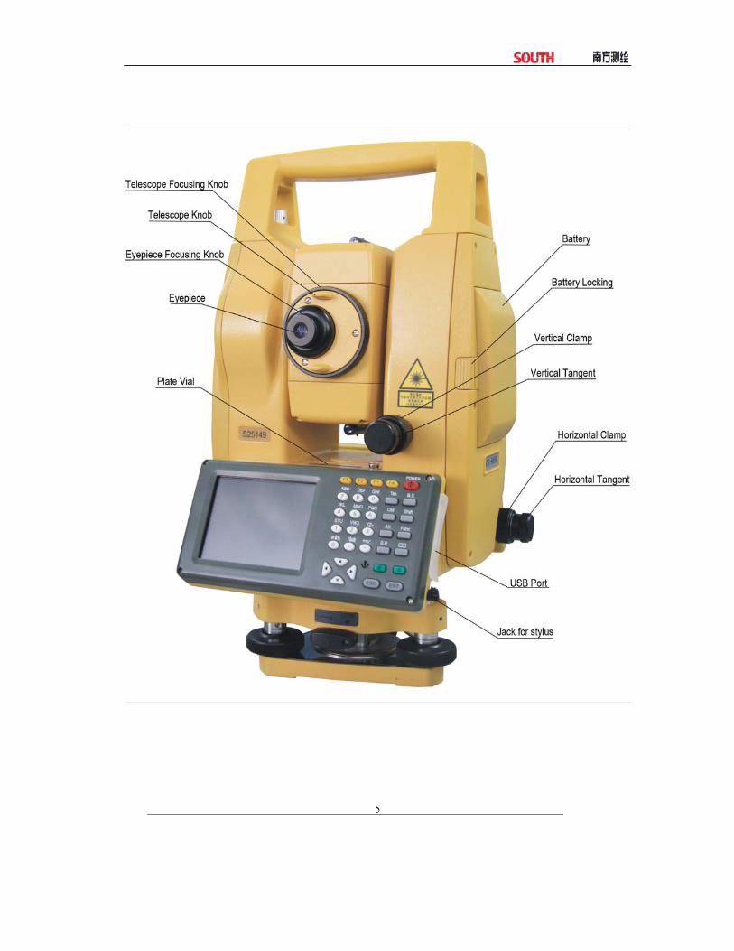
1. NOMENCLATURE AND FUNCTIONS 1.1 NOMENCLATURE
5

6
1.2 KEYPAD
Functions of the Keys
Key Nomenclature Function POWER Power Key To switch power ON/OFF.
F1~F4 Soft Key Refers to the function displayed.
0~9 Numeric Key To input desired numbers.
A~/ Alpha Key To input alphabets.
Tab Tab Key To move cursor rightward or to next character field.
B.S Backspace To delete one character leftward when inputting numbers or
alphabets.
Ctrl Ctrl Key Same as that on a PC.
Shift Shift Key Same as that on a PC.
Alt Alt Key Same as that on a PC.
Func Function Key To launch a specific function defined in the software.
S.P Space Key To input a space.
Inputting Panel
Key
To display inputting panel.
Cursor Key To move the cursor up/down/left/right.
α Alpha Shifting
Key
To shift to alphabet inputting mode.
★ Star Key To launch several comer functions of the instrument.
ESC ESC Key Quit to previous display or previous mode.
ENT Enter Key To finish and accept the data input.

7
2. SYNCHRONIZATION WITH PC 2.1 INSTALLATION MICROSOFT ACTIVESYNC
There is a CD of Microsoft ActiveSync attached in the product package. First, install Microsoft ActiveSync on the personal computer and communicate with PDA. Please follow the steps below. Before Installing Microsoft ActiveSync
Before installing, read the following words carefully: ●During the installation processing, reboot your computer is required. Therefore,
please save your jobs and quit all the applications before installation. ●To install Microsoft ActiveSync, you are supposed to have an USB cable
(available in the product package) connect the PDA with the personal computer. Installation Microsoft ActiveSync
● Put the CD into your disk drive. Microsoft ActiveSync Installation Guide will be run automatically. If it is not run,
double click on the “setup.exe” under the root menu in the disk drive. ● Click “Next” to install Microsoft ActiveSync.
2.2 CONNECTING TOTAL STATION WITH PC
After Installing Microsoft ActiveSync, restart your PC. ●Plug one end of the USB cable into the USB port beside the keypad of the total
station, and another end into one communication port on your PC. For detail, please, refer to your hardware manual.
●Switch total station on. The software will detect the PDA and setup the communication port. When it is connected successfully, the following message will display.

8
Using “Browse” Function After the synchronized between the total station and the PC, click “Browse” button to browse al the contents in the portable device (total station), as below.
You can assign a task to a file like delete or copy.
9
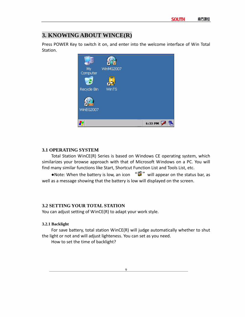
3. KNOWING ABOUT WINCE(R) Press POWER Key to switch it on, and enter into the welcome interface of Win Total Station.
3.1 OPERATING SYSTEM
Total Station WinCE(R) Series is based on Windows CE operating system, which similarizes your browse approach with that of Microsoft Windows on a PC. You will find many similar functions like Start, Shortcut Function List and Tools List, etc.
●Note: When the battery is low, an icon “ ”will appear on the status bar, as well as a message showing that the battery is low will displayed on the screen. 3.2 SETTING YOUR TOTAL STATION You can adjust setting of WinCE(R) to adapt your work style. 3.2.1 Backlight
For save battery, total station WinCE(R) will judge automatically whether to shut the light or not and will adjust lighteness. You can set as you need.
How to set the time of backlight?

10
OPERATIONAL STEPS KEY DISPLAY
①� On WindowsCE
desktop, click “Start”→“Settings”.
+
Settings
②Press control panel to enter into main menu. Use stylus to roll the slider bar to find “Display” icon.
Control panel
+
Display
③ Click “Display” to enter setting of Display Properties
④ Click “Backlight”, a function screen displays. Choose the time of turning off backlight to save battery. After setting, press [OK] to end.
Backlight
+
[OK]

11
3.2.2 Touch-screen Adjustment If the touch‐screen is not sense to the stylus, you need to adjust the touch‐screen. How to adjust touch‐screen?
OPERATION STEPS KEY DISPLAY ①� In “Control panel” find
“stylus” icon.
control panel
+
stylus
②Click “stylus”’
stylus
+
Calibration
③ Click “Calibration”, and then “Recalibrate”.
Calibration
+
Recalibrate
④According to the prompt, use the stylus to click the cross center. Repeat as the cross moves around the screen. Adjust 5 points as this.

12
⑤Press [ENT] to save new setting, Press [OK] to return to control panel.
[ENT]
+
[OK]
3.3 APPROACHES TO INPUT NUMERAL AND CHARACTER For Total Station WinCE(R) Series, Two kinds of inputting approaches are available. One is using the keyboard, like the keyboard of a mobile phone, with 3 characters on one key. Press it once to display the first characters. Press it twice to display the second one. And press it three times to display the third one. The other approach is using soft keyboard. Press icon [ ] to enter inputting interface. As an example, here we create a folder named “Job‐1”. [Example 1:Inputting via soft keyboard]
OPERATIONAL STEPS KEY DISPLAY
①� On desktop of WinCE,
press the blank area with the stylus for a while.
② Select “New Folder” on the pull-down menu appeared.

13
③On desktop of WinCE, a new folder is created. And activate the soft keyboard as seen on the right. ※1)
④Click the [Shift] key on the keyboard via the stylus to shift to capital letter inputting mode, as shown on the right. Click letter [J] to input a characters “J”.
[shift]
+
[J]
⑤ The system automatically returns to small letter inputting mode. Use the stylus to click characters key [o] and [b] to input “o” and “b”.
[o]
[b]
⑥ Click [-] to input “-”
[-]

14
⑦ Click number [1] to input “1”.
[1]
⑧ After inputting, click once on
the blank area on the desktop to
confirm the inputting and close the
soft keyboard.
※1) Input [ ] key to close soft keyboard.
[Example 2:Input via keyboard]
OPERATIONAL STEPS KEY DISPLAY ①� When a new folder is created
on the desktop, a soft keyboard
appears automatically. If a soft
keyboard is not needed, press
[ ] key to close the soft
keyboard, and use the numeric
keys on the instrument display
unit to input characters. ※1)
② Press [α] key to enter into
characters inputting mode. To input
capital letters, press [SHIFT] key,
as seen on the right, and press [4]
once to input a capital letter “J’.
[α]
[shift]
[4]
15
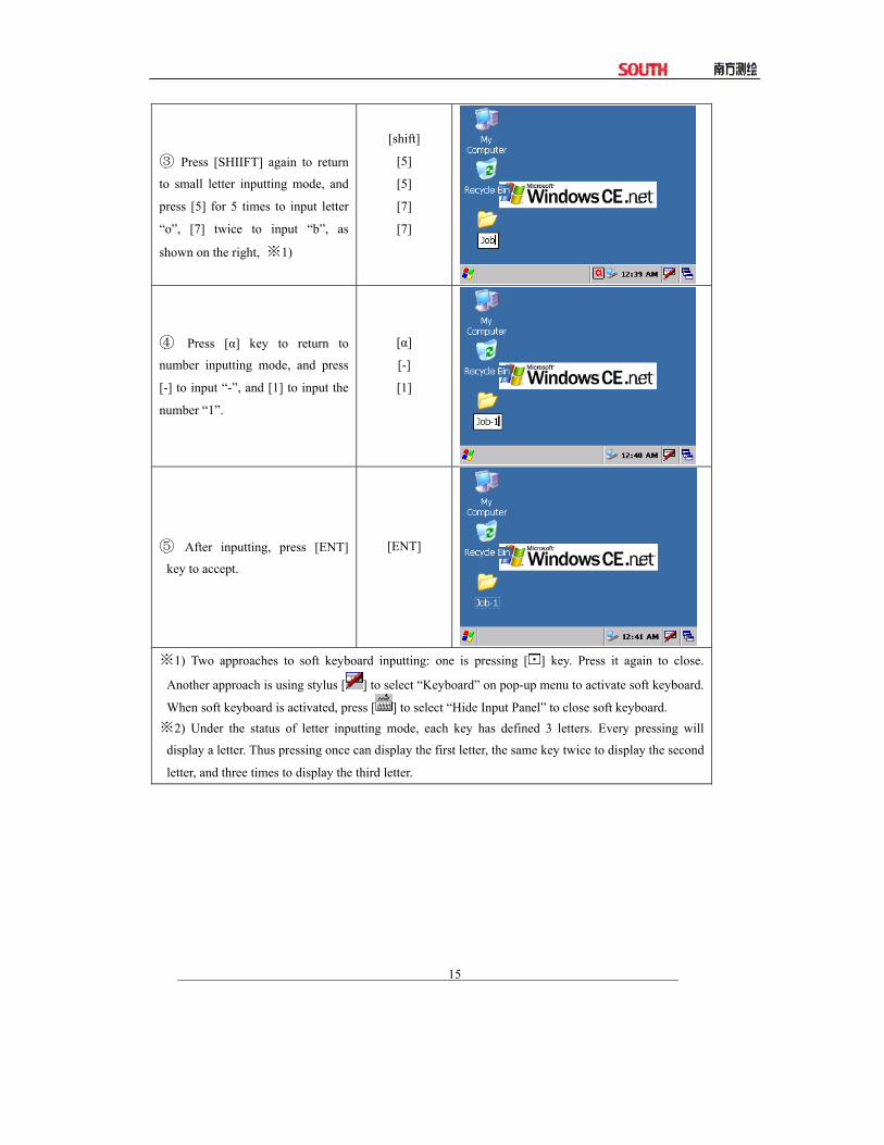
③ Press [SHIIFT] again to return
to small letter inputting mode, and
press [5] for 5 times to input letter
“o”, [7] twice to input “b”, as
shown on the right, ※1)
[shift]
[5]
[5]
[7]
[7]
④ Press [α] key to return to
number inputting mode, and press
[-] to input “-”, and [1] to input the
number “1”.
[α]
[-]
[1]
⑤ After inputting, press [ENT]
key to accept.
[ENT]
※1) Two approaches to soft keyboard inputting: one is pressing [ ] key. Press it again to close.
Another approach is using stylus [ ] to select “Keyboard” on pop-up menu to activate soft keyboard.
When soft keyboard is activated, press [ ] to select “Hide Input Panel” to close soft keyboard. ※2) Under the status of letter inputting mode, each key has defined 3 letters. Every pressing will
display a letter. Thus pressing once can display the first letter, the same key twice to display the second
letter, and three times to display the third letter.
16
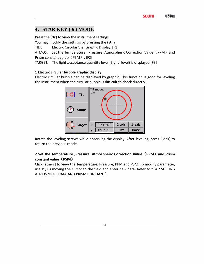
4.STAR KEY (★) MODE Press the (★) to view the instrument settings. You may modify the settings by pressing the (★): TILT: Electric Circular Vial Graphic Display. [F1] ATMOS: Set the Temperature , Pressure, Atmospheric Correction Value(PPM)and Prism constant value(PSM). [F2] TARGET: The light acceptance quantity level (Signal level) is displayed [F3] 1 Electric circular bubble graphic display Electric circular bubble can be displayed by graphic. This function is good for leveling the instrument when the circular bubble is difficult to check directly.
Rotate the leveling screws while observing the display. After leveling, press [Back] to return the previous mode. 2 Set the Temperature ,Pressure, Atmospheric Correction Value(PPM)and Prism constant value(PSM) Click [atmos] to view the Temperature, Pressure, PPM and PSM. To modify parameter, use stylus moving the cursor to the field and enter new data. Refer to “14.2 SETTING ATMOSPHERE DATA AND PRISM CONSTANT”.

17
3 Set the target type, illumination of cross hair and check the signal intensity. Click [Target], target type, illumination of cross hair, etc. can be set. Setting of target type: WinCE(R) Series total station can be set as red laser EDM and invisible infrared EDM, and the reflector can be set as with prism, without prism and reflecting sheet. User can set according to the requirement. WinCE Series total station has invisible infrared EDM function only, the prism used with which has to be matching with the prism constant. Use stylus to select among the options: reflectorless/sheet/ prism ●Refer to “ technical parameters” for the parameter of kinds of reflector.
Setting of illumination of cross hair: ●Move the stylus to adjust the brightness of crosshair. L: Indicate that the crosshair is dim. H: Indicate that the crosshair is bright Move the stylus from left to right to change the brightness of the crosshair from dim to bright. Setting of signal mode The reflector return signal intensity was displayed in this mode. It will buzzer when return signal from the prism was received. This function is more convenient for collimation when the target is difficult to find. The received return signal level is displayed with bar graph as follows.

18
No light acceptance Minimum quantity level Maximum quantity level
5. PREPARATION FOR MEASUREMENT 5.1 UNPACKING AND STORE OF INSTRUMENT ‐ Unpacking of instrument Place the case lightly with the cover upward, and unlock the case, take out the instrument. ‐ Store of instrument Cover the telescope cap, place the instrument into the case with the vertical clamp screw and circular vial upwards (Objective lens towards tribrach), and slightly tighten the vertical clamp screw and lock the case. 5.2 INSTRUMENT SETUP Put the instrument on the tripod. Level and center the instrument precisely to ensure the best performance.
Operation Reference: 1 Leveling and Centering the Instrument by plumb bob 1) Set up the tripod ① Extend the extension legs to suitable length, make the tripod head parallel to
the ground and tighten the screws. ② Make the centre of the tripod and the occupied point approximately on the

19
same plumb line. ③ Step the tripod to make sure if it is well stationed on the ground. 2) Put the instrument on the tripod Put the instrument carefully on the tripod head and slide the instrument by
loosening the tripod head screw. If the plumb bob is positioned right over the center of the point, slightly tighten the tripod head screw.
3) Roughly leveling the instrument by using the circular vial bubble. ① Turn the leveling screw A and B to move the bubble in the circular vial, in
which case the bubble is located on a line perpendicular to a line running through the centers of the two leveling screw being adjusted .
② Turn the leveling screw C to move the bubble to the center of the circular vial.
4) Precisely leveling by using the plate vial ① Rotate the instrument horizontally by loosening the Horizontal Clamp Screw
and place the plate vial parallel to the line connecting leveling screw A and B, and then bring the bubble to the center of the plate vial by turning the leveling screws A and B.
② Rotate the instrument 90º (100g) around its vertical axis and turn the remaining leveling screw or leveling C to center the bubble once more.
20
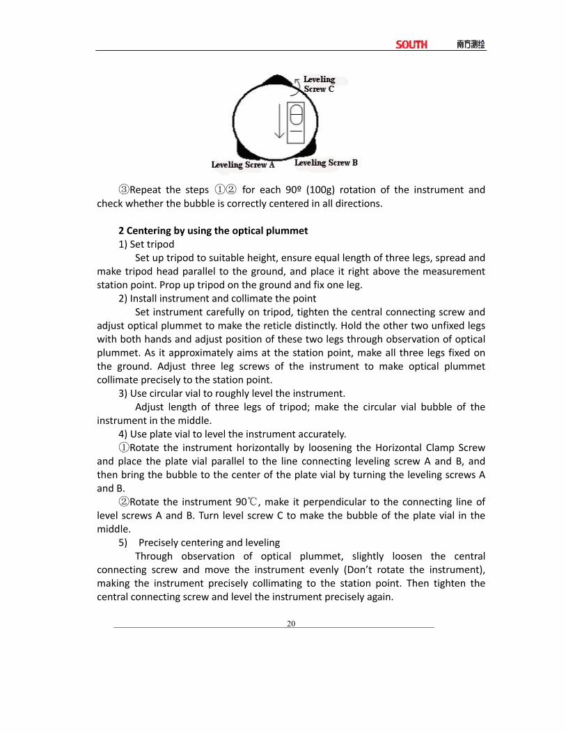
③Repeat the steps ①② for each 90º (100g) rotation of the instrument and check whether the bubble is correctly centered in all directions.
2 Centering by using the optical plummet 1) Set tripod Set up tripod to suitable height, ensure equal length of three legs, spread and
make tripod head parallel to the ground, and place it right above the measurement station point. Prop up tripod on the ground and fix one leg.
2) Install instrument and collimate the point Set instrument carefully on tripod, tighten the central connecting screw and
adjust optical plummet to make the reticle distinctly. Hold the other two unfixed legs with both hands and adjust position of these two legs through observation of optical plummet. As it approximately aims at the station point, make all three legs fixed on the ground. Adjust three leg screws of the instrument to make optical plummet collimate precisely to the station point.
3) Use circular vial to roughly level the instrument. Adjust length of three legs of tripod; make the circular vial bubble of the
instrument in the middle. 4) Use plate vial to level the instrument accurately. Rotate the instrument horizontally by loosening the Horizontal Clamp Screw ①
and place the plate vial parallel to the line connecting leveling screw A and B, and then bring the bubble to the center of the plate vial by turning the leveling screws A and B.
②Rotate the instrument 90 , make it perpendicular to the connecting line of ℃level screws A and B. Turn level screw C to make the bubble of the plate vial in the middle.
5) Precisely centering and leveling Through observation of optical plummet, slightly loosen the central
connecting screw and move the instrument evenly (Don’t rotate the instrument), making the instrument precisely collimating to the station point. Then tighten the central connecting screw and level the instrument precisely again.
21
Repeat this operation till the instrument collimate precisely to the measurement station point.
5.3 BATTERY INFORMATION
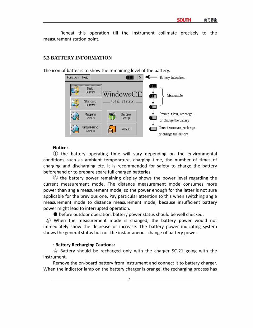
The icon of batter is to show the remaining level of the battery.
Notice: ① the battery operating time will vary depending on the environmental
conditions such as ambient temperature, charging time, the number of times of charging and discharging etc. It is recommended for safety to charge the battery beforehand or to prepare spare full charged batteries.
② the battery power remaining display shows the power level regarding the current measurement mode. The distance measurement mode consumes more power than angle measurement mode, so the power enough for the latter is not sure applicable for the previous one. Pay particular attention to this when switching angle measurement mode to distance measurement mode, because insufficient battery power might lead to interrupted operation.
● before outdoor operation, battery power status should be well checked. ③ When the measurement mode is changed, the battery power would not immediately show the decrease or increase. The battery power indicating system shows the general status but not the instantaneous change of battery power.
∙ Battery Recharging Cautions: ☆ Battery should be recharged only with the charger SC‐21 going with the
instrument. Remove the on‐board battery from instrument and connect it to battery charger.
When the indicator lamp on the battery charger is orange, the recharging process has

22
begun. When charging is complete (indicator lamp turns green), disconnect the charger from its power source.
∙Battery Removal Cautions: Before removing the battery from the instrument, make sure that the power is
turned off. Otherwise, the instrument may be damaged. ∙Battery Recharging Cautions: The charger has built‐in circuitry for protection from overcharging. However, do
not leave the charger plugged into the power outlet after recharging is completed. Be sure to recharge the battery at a temperature of 0°~±45°C, recharging may
be abnormal beyond the specified temperature range . When the indicator lamp does not light after connecting the battery and charger,
either the battery or the charger may be damaged. Please connect professionals for repairing.
∙Battery Charging Cautions: Rechargeable battery can be repeatedly recharged 300 to 500 times. Complete
discharge of the battery may shorten its service life. In order to get the maximum service life, be sure to recharge it at least once a
month. 5.4 REFLECTOR PRISM When measuring distance, a reflector prism needs to be placed at the target place. Reflector systems come with single prism and triple prisms, which can be mounted with tribrach onto a tripod or mounted onto a prism pole. Reflector systems can be self‐configured by users according to job.
5.5 MOUNTING AND DISMOUNTING INSTRUMENT FROM TRIBRACH

23
∙Dismounting If necessary, the instrument (including reflector prisms with the same tribrach) can be dismounted from tribrach. Loosen the tribrach locking screw in the locking knob with a screwdriver. Turn the locking knob about 180° counter‐clockwise to disengage anchor jaws, and take off the instrument from tribrach.
∙Mounting Insert three anchor jaws into holes in tribrach and line up the directing stub with the directing slot. Turn the locking knob about 180°clockwise and tighten the locking screw with a screwdriver. 5.6 EYEPIECE ADJUSTMENT AND COLLIMATING OBJECT Method of Collimating Object(for reference)
① Sight the Telescope to bright place and rotate the eyepiece tube to make the reticle clear.
② Collimate the target point with top of the triangle mark in the coarse collimator. (Keep a certain distance between eye and the coarse collimator).
③Make the target image clear with the telescope focusing screw. ☆ if there is parallax when your eye moves up, down or left, right, it means the diopter of
eyepiece lens or focus is not well adjusted and accuracy will be influenced, so you should adjust

24
the eyepiece tube carefully to eliminate the parallax.
5.7 VERTICAL AND HORIZONTAL ANGLE TILT CORRECTION When the tilt sensors are activated, automatic correction of vertical and
horizontal angle for mislevelment is displayed. To ensure a precise angle measurement, tilt sensor must be turned on. When a
dialog of compensation displays, it indicates that the instrument is out of automatic compensation range (±4 ), and must be leveled manually.′
WinCE(R) Series compensates both the vertical and horizontal angle readings due to inclination of the standing axis in the X and Y direction. Example:`
OPERATIONAL STEPS KEY DISPLAY
①� If the instrument hasn’t been
leveling, a compensation
dialog box will pop up
automatically. As shown in the
right graph.
②Turn the leveling screw to make
the small block dot move into the
small circle.
When the small black dot is in the
small circle, it means the instrument
is within the auto tilt compensation
scale ±4′.
If it is outside the small circle, the
instrument needs to be leveled
manually.
③ To set it to single axis
compensation, click [1-axis]; To
close compensation, click [OFF];
To return to previous mode, click
[Back].
● the display of vertical and horizontal angle is unstable when instrument is on an unstable stage or is used during a windy day. You can turn off the auto tilt correction function of V/H angle in this case.

25
● If the Tile Correction is ON (Single Axis or Dual Axis), under the situation that the instrument is not well leveled, you can level the instrument according to the moving direction of the electronic bubble as seen on above.
6. BASIC SURVEY
On desktop of WinCE double click to enter into the menu of Win Total Station, as shown in the following graph:
You can press numeric keys [1]~[5] to select functions. To quit this screen, press [ESC].
Press numeric key [1] or click “ ” to enter into basic survey. The screen displays as follows.
Description of each function key: Function keys display at the bottom of the screen, which change with the measure
Mode key
Current
Function

26
mode. The following graph lists each function key in every measure mode.
Mode Display Softkey Function
0 Set 1 0 Set horizontal angle.
HSet 2 Preset a horizontal angle.
Hold 3 Hold horizontal angle.
Repeat 4 Repeat horizontal angle measurement.
V% 5 Switch between vertical angle and percentage.
HR/HL 6 Switch horizontal angle right/left
Mode 1 EDM mode: Fine[s]/ Fine[N]/ Fine [r]/Track
m/ft 2 Distance unit: meter/Feet/U.S.
Layout
3 Layout measure mode
REM 4 Start Remote Elevation Measurement.
MLM 5 Start Missing Line Measurement.
Line Ht 6 Start Line Height Measurement.
Mode 1 EDM mode: Fine[s]/ Fine[N]/ Fine [r]/Track
Occ 2 Preset coordinates of occupied point.
BS 3 Preset coordinates of backsight point.
Setup 4 Preset instrument height and target height.
Store 5 Start store function.
Offset 6 Start Offset measurement. (Angle Offset (1) /Distance
Offset (2)/Column Offset (3)/Plane Offset (4)).
6.1 ANGLE MEASUREMENT 6.1.1 Horizontal Angle (Right Angle) and Vertical Angle Measurement Make sure the mode is Angle measurement.

27
OPERATIONAL STEPS KEY DISPLAY
①Sight the first target A.
Sight target A
②Set the horizontal angle of target
A as 0°00′00″.
Click [0 SET], press [OK] in the
pop-up dialog box to confirm.
[0 Set]
[OK]
③Sight second target (B).
The screen displays the horizontal
and vertical angle of target B.
Sight B
How to collimate the targets (For reference) ① Point the telescope toward the light,rotate the eyepiece ring,focalize the telescope so that the crosshair is clearly observed(turn the eyepiece ring to you first and then to focus). ② Aim the target at the peak of triangle mark of the collimator. Keep a certain space between the collimator and yourself for collimation. ③ Focus the target with the focusing knob until the target is clearly seen and its center is right on the crosshair. If parallax exists between the crosshair and the target when viewing vertically or horizontally through the telescope, focusing is incorrect or diopter adjustment is poor. This adversely affects precision in measurement or survey. So please eliminate the parallax by focusing and using diopter adjustment carefully.
6.1.2 Switch Horizontal Angle Right/Left Make sure the mode is Angle measurement.
28
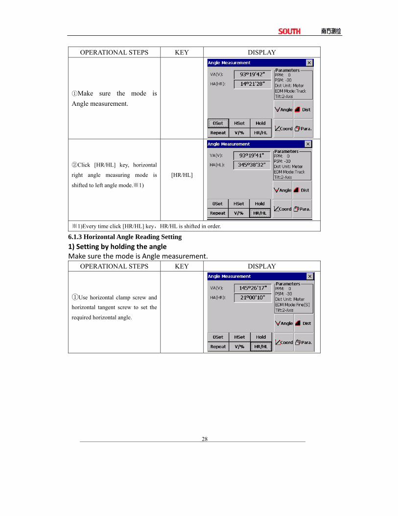
OPERATIONAL STEPS KEY DISPLAY
①Make sure the mode is Angle measurement.
②Click [HR/HL] key, horizontal
right angle measuring mode is
shifted to left angle mode.※1)
[HR/HL]
※1)Every time click [HR/HL] key,HR/HL is shifted in order.
6.1.3 Horizontal Angle Reading Setting 1) Setting by holding the angle Make sure the mode is Angle measurement.
OPERATIONAL STEPS KEY DISPLAY
①Use horizontal clamp screw and
horizontal tangent screw to set the
required horizontal angle.
29
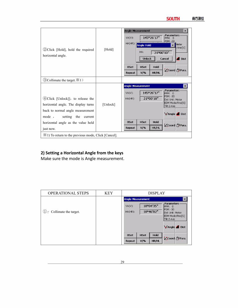
②Click [Hold], hold the required
horizontal angle.
[Hold]
③Collimate the target.※1)
④Click [Unlock]],to release the
horizontal angle. The display turns
back to normal angle measurement
mode , setting the current
horizontal angle as the value held
just now.
[Unlock]
※1) To return to the previous mode, Click [Cancel].
2) Setting a Horizontal Angle from the keys Make sure the mode is Angle measurement.
OPERATIONAL STEPS KEY DISPLAY
①� Collimate the target.

30
②Click [HSet],a dialog box pops
up.
③ Input the required horizontal
angle※1)、※2)
For Example: 120°00′00″
[HSet]
Input
horizontal
angle
④After inputting, press [ENT]※
3)
When completed, normal
measuring from the required
Horizontal angle is possible.
[ENT]
※1) You can press [ ] to open inputting panel, click the numbers to input,see “3.3 APPROACHES TO
INPUTTING NUMBERS AND LETTERS”.
※2) To revise wrong value, use stylus or press [ ]/ [ ] moving the cursor to right of the number need
to delete. Click [ ] on the panel or press [B.S.] to delete wrong value and input correct one.
※3) With wrong input value (for example 70′), Setting failed, press [ENT], the system doesn’t respond,
input again from step ③.
6.1.4 Vertical Angle Percentage (%) Mode Make sure the mode is Angle measurement. Example:
OPERATIONAL STEPS KEY DISPLAY
①Make sure the mode is Angle
measurement.

31
②Click [V/%]. ※1)
[V%]
※1) Every time Click [V/%], the display mode switches accordingly.
6.1.5 Repeat Angle Measurement
This program is used to accumulate repeated angle measurement, displaying the sum of and average value of all observed angles. It records the observation times at the same time.
Example: OPERATIONAL STEPS KEY DISPLAY
① Click [Repeat] to enter into
Angle Repeat function.
[Repeat]

32
②Sight the first target A.
Sight target A
③ Click [0 Set], 0 Set the
horizontal angle.
[0 Set]
④Use horizontal clamp screw and
horizontal tangent to sight the
second target B.
Sight B
⑤Click [Hold].
[Hold]

33
⑥Use horizontal clamp screw and
horizontal tangent to sight first
target A again.
⑦Click [Unlock].
Sight A again
+
[Unlock]
⑧Use horizontal clamp screw and
horizontal tangent to sight the
second target B again.
⑨Click [Hold].
The total of angle (Ht) and the
mean value of angle (Hm) are
shown.
Sight B again
[Hold]
⑩Repeat ⑥~⑨ to reach the
desired number of repetition. ※1)
※1) Click [Exit] to quit angle repeat measurement.
6.2 DISTANCE MEASUREMENT In basic surveying screen, click [Dist] to enter into distance measurement.
NOTE: Measurements to strongly reflecting targets such as to traffic lights in infrared mode
34
should be avoided. The measured distances may be wrong or inaccurate. When the [MEASURE] is triggered, the EDM measures the object which is in the beam path at that moment. If e.g. people, cars, animals, swaying branches, etc. cross the laser beam while a measurement is being taken, a fraction of the laser beam is reflected and may lead to incorrect distance values.
Avoid interrupting the measuring beam while taking reflectorless measurements or measurements using reflective foils.
Reflectorless EDM Ensure that the laser beams cannot be reflected by any object nearby with ●
high reflectivity. When● a distance measurement is triggered, the EDM measures to the object
which is in the beam path at that moment. In case of temporary obstruction (e.g. a passing vehicle, heavy rain, snow, frog, etc.), the EDM may measure to the obstruction.
●When measuring longer distance, any divergence of the red laser beam from the line of sight might lead to less accurate measurements. This is because the laser beam might not be reflected from the point at which the crosshairs are pointing. Therefore, it is recommended to verify that the R‐laser is well collimated with the telescope line of sight. (Please refer to “****”REFLECTORLESS EDM”)
Do not collimate the same target with the 2 total stations● simultaneously. Accurate measurements to prisms should be made with the standard program
(infrared mode). Red Laser Distance Measurement Cooperated with Reflective Foils.
The visible red laser beam can also be used to measure to reflective foils. To guarantee the accuracy the red laser beam must be perpendicular to the reflector foil and it must be well adjusted (refer to “****” REFLECTORLESS EDM”). Make sure the additive constant belongs to the selected target (reflector). 6.2.1 Setting Atmosphere Correction
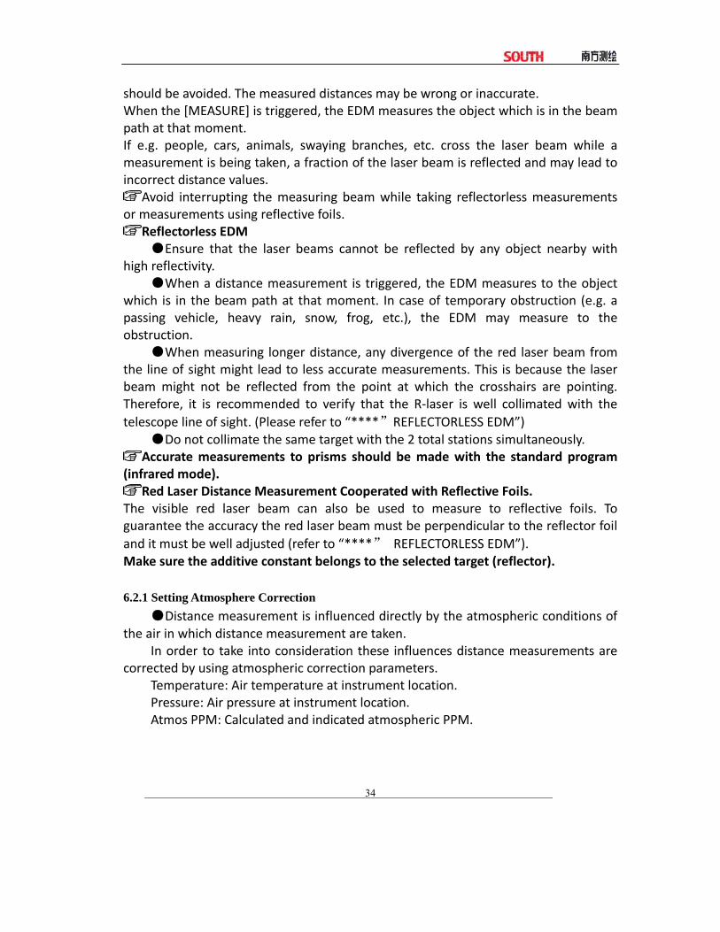
●Distance measurement is influenced directly by the atmospheric conditions of the air in which distance measurement are taken.
In order to take into consideration these influences distance measurements are corrected by using atmospheric correction parameters.
Temperature: Air temperature at instrument location. Pressure: Air pressure at instrument location. Atmos PPM: Calculated and indicated atmospheric PPM.
35
6.2.1.1 Calculation of Atmospheric Correction ●The value of Atmospheric Correction can be influnced by air pressure, air temperature and the height. The calculating formula is as follows: (calculating unit:meter)
PPM = 273.8 ‐ 0.2900 × Pressure Value(hPa) 1 + 0.00366 × Temperature value(℃)
If the pressure unit adopted is mmHg: make conversion with: 1hPa = 0.75mmHg.
●The standard atmospheric condition of WinCE Series (e.g. the atmospheric condition under which the atmospheric correction value of the instrument is zero ) : Pressure:1013 hPa Temperature: 20℃
If regardless of atmospheric correction, please set PPM value as 0.
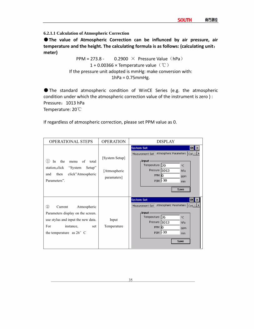
OPERATIONAL STEPS OPERATION DISPLAY
① In the menu of total
station,click “System Setup”
and then click”Atmospheric
Parameters”.
[System Setup]
[Atmospheric
paramaters]
② Current Atmospheric
Parameters display on the screen.
use stylus and input the new data.
For instance, set
the temperature as 26°C
Input
Temperature

36
③According to the same steps,
input the value of Air pressure.
click the “Save” after finishing
setting.
Input Pressure
+
[Save]
④ Press [OK] to save these
parameters. System will get PPM
value from the value of
temperature and air pressure, The
screen displays as the right
graph.
[OK]
※1The inputting scope:Temperature:-30~+60℃(step length 0.1℃) or -22~+140℉(step length 1℉) Air pressure:420 ~ 800 ㎜ Hg(step length 1 ㎜ Hg) or 560 ~ 1066 hPa(step length 0.1hpa)
16.5 ~ 31.5 inchHg(step length 0.1 inchHg)
Atmospherie parameters(PPM): -100~+100ppm (step length 1 ppm)
※2)The atmosphere correction value will be calculated by the instrument according to the inputted
temperature and pressure value.
6.2.1.2, Input Atmospheric Correction Value directly Test the temperature and air pressure out,and get the Atmospheric Correction Value(PPM) from the formula of Atmospheric Correction.

37
OPERATIONAL STEPS OPERATION DISPLAY
①In the menu of total station,
click “System Setup” and then
click ”Atmospheric Parameters”
“System Setup”
+“Atmospheric
Parameters
②Delete the old PPM and input
the new one※1) Input PPM Value
③Click [Save] to save the value. [Save]
※1)The inputting scope of Atmospherie parameters :-100 ~ +100 PPM(step length : 1PPM)
Atmospheric Correction value also can be set in star key (★)model. 6.2.2 Atmospheric Refraction And Earth Curvature Correction
The instrument will automatically correct the effect of atmosphere refraction and the earth curvature when calculating the horizontal distance and the height differences.
The correction for atmosphere refraction and the earth curvature are done by the formulas as follows: Corrected Horizontal Distance: D=S * [cosα+ sinα* S * cosα(K‐2) / 2Re] Corrected Height Differentia:

38
H= S * [sinα + cosα* S * cosα(1‐K) / 2Re] If the correction of atmosphere refraction and the earth curvature is neglected, the calculation formula of horizontal distance and the height differentia are: D=S·cosα H=S·sinα
In formula: K=0.14 ……………………Atmosphere Refraction Modulus
Re=6370 km ………………The Earth Curvature Radius
α(orβ) ………………...The Vertical Angle Calculated From Horizontal Plane (Vertical Angle)
S ………………………….Oblique Distance NOTE: The atmosphere refraction modulus of this instrument has been set as:
K=0.14.it als can be set as :K=0.2,or be set shut (0 VALUE).(refer to “****”SYSTEM SETTINGS)
6.2.3 Setting Target Type WinCE(R) Series Total Stations can set options of Red Laser(RL) EDM and Invisible Laser(IL) EDM, as well as reflector with prism, non‐prism, and reflective foil. User can set them according to the requirements of the job.WinCE Series Total Stations are only equipped with laser EDM function,which requires that the prism is in accordance with the prism constant. You can set Target Type in star key (★)model.
OPERATIONAL STEPS OPERATION DISPLAY
①Press[★] on keypad to enter into
star key mode. [☆]

39
②Click [Target] to enter into the
function of setting type of the
target.
[Target]
③4. Use stylus to choose the type
of the target. Non-Prism,
Sheet,Prism options can be chose
under WinCE(R) total station.※1)
④Press [ENT] to quit.
[ENT]
※1) Instrucion of the target type:
Non-P: measure with the visible red laser, no need to use prism. All of types of target are
available for measure.
Sheet: Use the sheet as target to measure.
Prism: Use the prism as target to measure.
6.2.4Setting the Prism Constant Since the constants of prisms manufactured by different companies are different, the corresponding prism constant must be set. Once the prism constant is set, it would be kept even if the machine is turned off.
OPERATIONAL STEPS OPERATION DISPLAY
①In the menu of total station,
click “System Setup”and then
click “Atmospheric Parameters”
“System Setup”
+
“Atmospheric
Parameters”

40
② Current Atmospheric
Parameters display on the screen.
Use stylus to move cursor to
PSM input area, delete data and
input new numbers.※1)
Input Value
③Click [Save].
[Save]
④Click [OK] to save. [OK]
※1) The scope of prism constant :-100mm~+100mm, Step Length 0.1mm
.You also can set Prism Constant in star key (★)model. 6.2.5Distance Measurement (Continue Measurement) Make sure the mode is Angle measurement.
OPERATIONAL STEPS KEY DISPLAY
①Sight the center of prism.
Sight
41
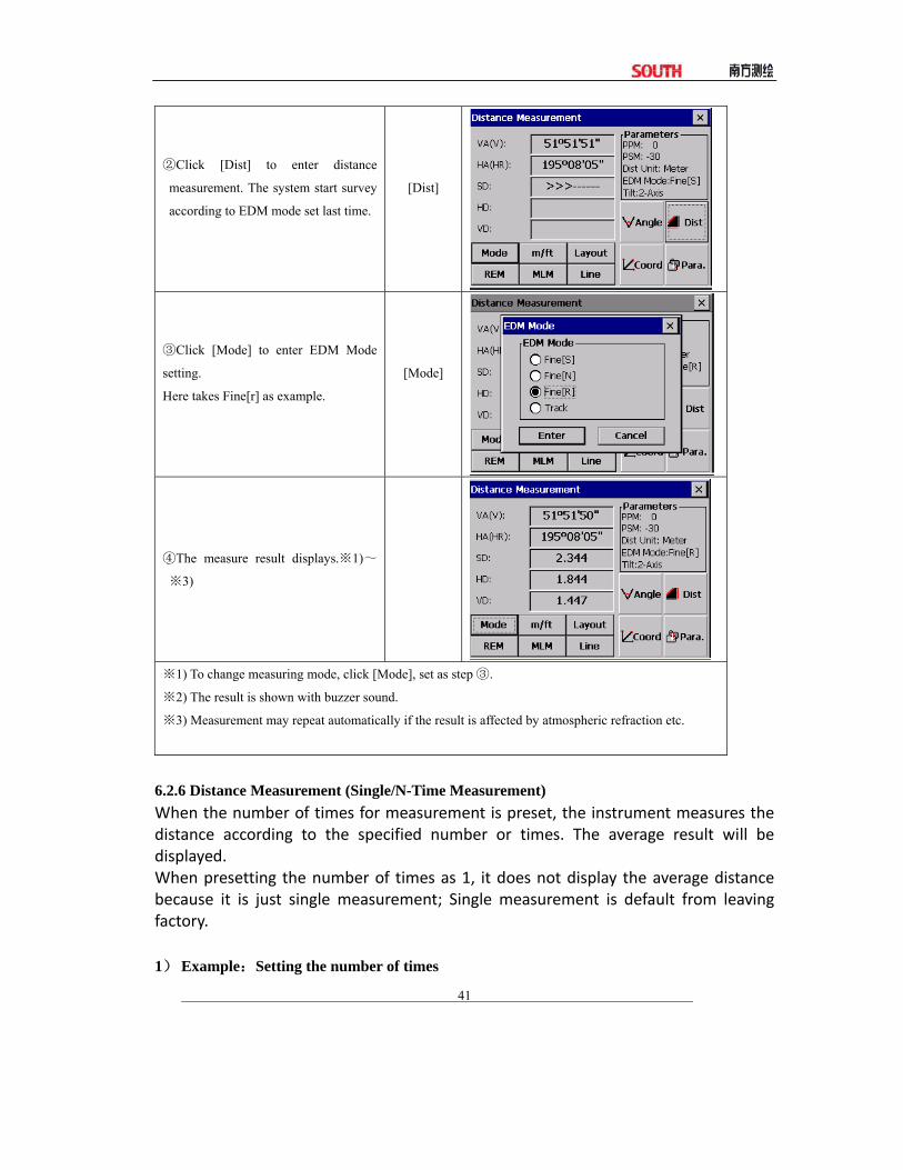
Click [Dist] to enter distance ②
measurement. The system start survey
according to EDM mode set last time.
[Dist]
Click [M③ ode] to enter EDM Mode
setting.
Here takes Fine[r] as example.
[Mode]
The measure result displays. 1)④ ※ ~
※3)
1) To change measuring mode, click [Mode], set as step .※ ③ 2) The result is shown with buzzer sound.※
3)※ Measurement may repeat automatically if the result is affected by atmospheric refraction etc.
6.2.6 Distance Measurement (Single/N-Time Measurement) When the number of times for measurement is preset, the instrument measures the distance according to the specified number or times. The average result will be displayed. When presetting the number of times as 1, it does not display the average distance because it is just single measurement; Single measurement is default from leaving factory. 1) Example:Setting the number of times

42
OPERATIONAL STEPS KEY DISPLAY
In EDM Mode, click [Mode] to ①
enter EDM Mode setting.
System defaults as Fine[s].
[Mode]
Click Fine [N] or press [▲]/ ②
[▼], a Times column displays on
the upper right screen. Input the
times of N-time measurement.
[Fine[N]]
Input times
Click [Enter]. Sight the target, ③
system start survey based on the
setting set just now.
[Enter]
6.2.7Fine/Tracking Measurement Mode Fine mode: This is the normal distance measurement mode. Tracking mode: This mode measures in a shorter time than in fine mode. Use this mode for stake‐out measurement. It is very useful for tracing the moving object or carrying out engineering stake‐out job. Example:
43
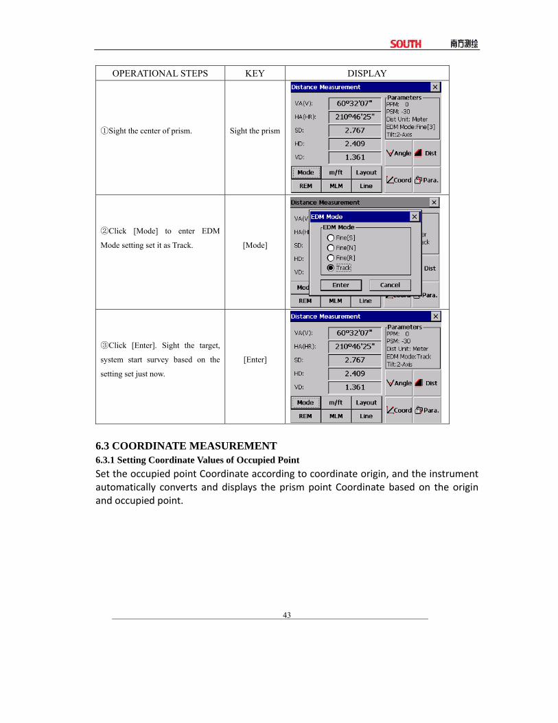
OPERATIONAL STEPS KEY DISPLAY
Sight the center of prism.①
Sight the prism
Click [Mode] to enter EDM ②
Mode setting set it as Track.
[Mode]
Click [Enter]. Sight the target, ③
system start survey based on the
setting set just now.
[Enter]
6.3 COORDINATE MEASUREMENT 6.3.1 Setting Coordinate Values of Occupied Point Set the occupied point Coordinate according to coordinate origin, and the instrument automatically converts and displays the prism point Coordinate based on the origin and occupied point.

44
Example: OPERATIONAL STEPS KEY DISPLAY
① Click [Coord] to enter into
coordinate measurement.
[Coord]
②Click [Occ] .
[Occ]
③ Input coordinate of occupied
point, after inputting one item,
click [Enter] to move to the next
item.
[Enter]
45
④After all inputting, click [Enter]
to return to coordinate measurement
screen.
[Enter]
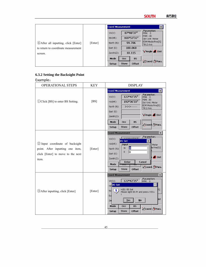
6.3.2 Setting the Backsight Point Example:
OPERATIONAL STEPS KEY DISPLAY
①Click [BS] to enter BS Setting.
[BS]
② Input coordinate of backsight
point. After inputting one item,
click [Enter] to move to the next
item.
[Enter]
③After inputting, click [Enter]
[Enter]
46
④Sight the backsight point, click
[YES]. System sets the backsight
azimuth and returns to Coordinate
Measurement Screen. The screen
displays the backsight azimuth set
just now.
[Yes]
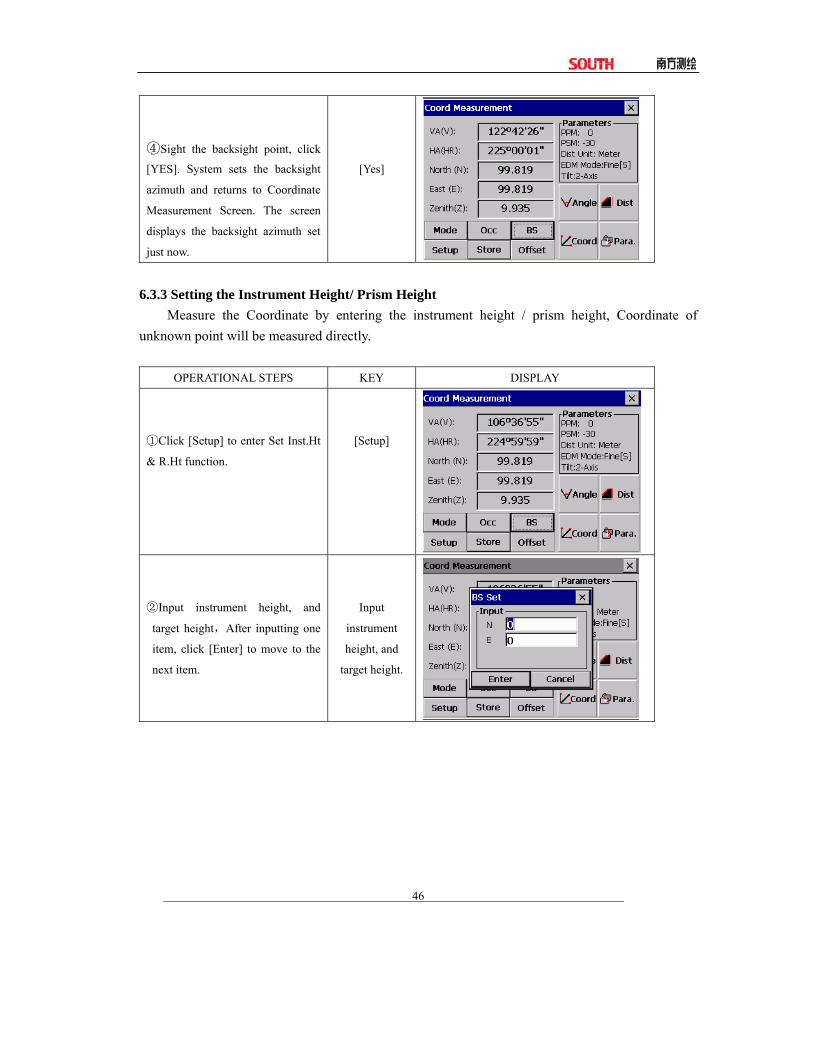
6.3.3 Setting the Instrument Height/ Prism Height
Measure the Coordinate by entering the instrument height / prism height, Coordinate of unknown point will be measured directly.
OPERATIONAL STEPS KEY DISPLAY
Click [Setup] to enter Set Inst.Ht ①
& R.Ht function.
[Setup]
Input instrument height, and ②
target height,After inputting one
item, click [Enter] to move to the
next item.
Input
instrument
height, and
target height.

47
After inpu③ tting all data, Click
[Enter] to return to Coordinate
Measurement Screen.
[Enter]
6.3.4 Operation of Coordinate Measurement Measure the Coordinate by entering coordinate of occupied point, backsight azimuth, the instrument height and prism height, coordinate of unknown point will be measured directly. ●To set coordinate value of occupied point,see Section “6.3.1 Setting Coordinate Values of Occupied
Point”. ●To set the instrument height and prism height,see Section “6.3.3 Setting of the Instrument
Height/Prism Height”. ●The Coordinate of the unknown point are calculated as shown below and displays: Coordinate of occupied point:(N0, E0, Z0) Coordinate of the centre of prism ,originated from the centre point of the instrument:(n,e,z) Coordinate of unknown point :(N1,E1,Z1) N1 = N0 + n E1 = E0 + e Z1 = Z0 + Inst.Ht + z –Prism .h
Example:

48
OPERATIONAL STEPS KEY DISPLAY
①Set coordinate values of occupied
point and instrument / prism height
1)※
Set backsight azimuth② 。 2)※
③Collimate target. ※3)
Click [Coord]. Measurement ④
ends and the result displays. 4)※
[Coord]
1)※ In case the coordinate of occupied point is not entered, then the coordinate of occupied point set
last time would be used. The instrument height and the prism height will be the value you set last time.
2)※ Refer to Section “6.1.3 Horizontal Angle Reading Setting” or “6.3.2 Setting the Backsight Point”.
3)Click[Mode]※ ,the mode (SINGLE/N-TIME/REPEAT/TRACKING) changes .
4)※ To return to the normal angle or distance measuring mode, click [Angle]/ [Dist].
7. APPLICATION PROGRAMS 7.1 LAYOUT
The difference between the measured distance and the preset distance is displayed. The displayed value = Measured distance – Standard (Preset) distance
● This function enables the stake-out of Horizontal Distance (HD), Vertical Difference (VD) or Slope Distance (SD) . Example:

49
OPERATIONAL STEPS KEY DISPLAY
Under the mode of Distance ①
Measurement, click [Layout].
[Layout]
Select the distance measurement ②
mode (SD/HD/VD) to be laid out.
After inputting the data to be laid
out, click [Enter] 1)※
③ Start setting out.
1)※ A dialog box prompts to enter slope distance you want to layout, after entering click[Enter] to
layout SD. To layout horizontal distance, input 0 in SD dialog box. Click [Enter], the HD box will
prompt. After entering click [Enter] to layout HD. To layout height difference, input 0 in SD and HD
box, and then the dialog box of VD to be staked out will prompt.
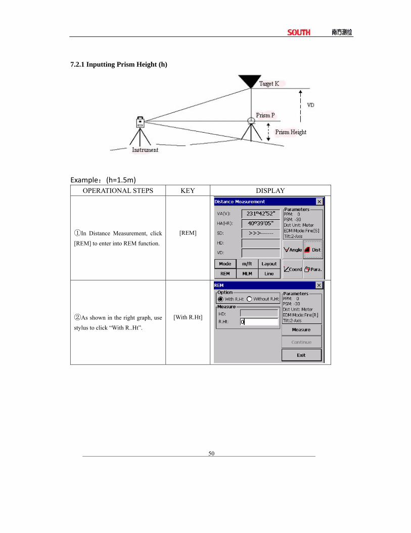
7.2 REMOTE ELEVATION MEASUREMENT (REM)
The Remote Elevation program calculates the vertical distance (height) of a remote object relatively to a prism and its height from a ground point (without a prism height). When using a prism height, the remote elevation measurement will start from the prism (reference point). If no prism height is used, the measurement will start from any reference point in which the vertical angle is established. In both procedures, the reference point should be perpendicular to the remote object.
50
7.2.1 Inputting Prism Height (h)
Example:(h=1.5m)
OPERATIONAL STEPS KEY DISPLAY
①In Distance Measurement, click
[REM] to enter into REM function.
[REM]
②As shown in the right graph, use
stylus to click “With R..Ht”.
[With R.Ht]

51
③Input prism height.
Input prism
height
④Sight the prism center P.
⑤Click [Measure] to start measure.
⑥The HD betweent instrument and
prism is displayed.
Sight the prism
[Measure]
⑦ Click [Continue], the prism
position is entered.
[Continue]
⑧Sight target K.
The Vertical Distance (HD) is
displayed. ※1)
Sight K
※1) To quit REM, click [Exit].
7.2.2 without Inputtingt Prism Height

52
Example:
OPERATIONAL STEPS KEY DISPLAY
①Use stylus to click “Without R.
Ht”
Without R.Ht
②Sight prism center P.
③Click [Measure] to start survey.
④The HD between instrument and
prism is displayed.
Sight prism
[Measure]
⑤Click [Continue],
The G point position is entered.
[Continue]

53
⑥Click [Continue].
[Continue]
⑦Sight target K.
The Vertical Distance (VD) is
displayed. ※1)
Sight target
※1) To quit REM, click [Exit].
7.3 MISSING LINE MEASUREMENT (MLM) The Missing Line Measurement program computes the horizontal distance (dHD), slope distance (dSD) and vertical difference (dVD). This program can accomplish this in two ways: 1.(A‐B,A‐C):Measurement A‐B,A‐C,A‐D …… 2.(A‐B,B‐C):Measurement A‐B,B‐C,C‐D ……
[EXAMPLE] 1. (A‐B,A‐C)

54
OPERATIONAL STEPS KEY DISPLAY
①In Distance Measurement, click
[MLM] to enter into missing line
measurement function
[MLM]
②Use stylus to select A-B,A-C.
③Sight prism A, click [Measure].
The HD between instrument and
prism A is displayed.
[Measure]
④Click [Continue].
[Continue]

55
⑤Sight prism B,Click [Measure]].
[Measure]
⑥Click [Continue], The horizontal
distance (dHD) height differentia
(dVD) and slope distance (dSD)
between prism A and B display.
※1)
[Continue]
⑦ To measure distance between
point A and C, sight prism C and
then click [Meas. After measuring,
horizontal distance between the
instrument and prism C displays.
[Measure]
⑧Click [Continue], the horizontal
distance (dHD) height differentia
(dVD) and slope distance (dSD)
between prism A and C display.
[Continue]
※1) Click [Exit] to return to main menu.
●The observation procedure of (A‐B,B‐C) is same as (A‐B,A‐C).
56
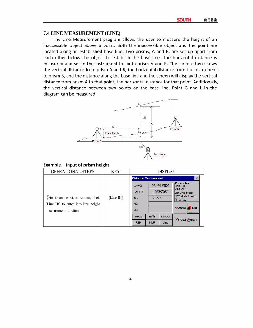
7.4 LINE MEASUREMENT (LINE) The Line Measurement program allows the user to measure the height of an
inaccessible object above a point. Both the inaccessible object and the point are located along an established base line. Two prisms, A and B, are set up apart from each other below the object to establish the base line. The horizontal distance is measured and set in the instrument for both prism A and B. The screen then shows the vertical distance from prism A and B, the horizontal distance from the instrument to prism B, and the distance along the base line and the screen will display the vertical distance from prism A to that point, the horizontal distance for that point. Additionally, the vertical distance between two points on the base line, Point G and L in the diagram can be measured.
Example:Input of prism height
OPERATIONAL STEPS KEY DISPLAY
①In Distance Measurement, click
[Line Ht] to enter into line height
measurement function
[Line Ht]

57
②Use stylus select with R.H.
③ Click [Set] to set instrument
height and target height. After
inputting, click [Enter].
[Set]
④Sight prism A, click [Meas] to
start measure. After measuring,
click [Continue].
[Meas]
⑤Sight prism B, click [Meas] to
start distance measure.
[Meas]

58
⑥ After measuring click
[Continue].
[Continue]
⑦ Sight line point L, Measured
data to the line point L is diplayed.
VD : Vertical distance
HD: Horizontal distance from the
instrument to L
Off : Horizontal distance from A to
L
⑧Click [Continue].
This function is used when
measuring the line height from the
groud OPERATIONAL STEPS:
●Sight the point on the line before
clicking [Next].
●Don't move the horizontal tangent
screw by setting groud point G
[Continue]
⑨Rotate the vertical tangent screw
and sight groud point G.
Sight G
59
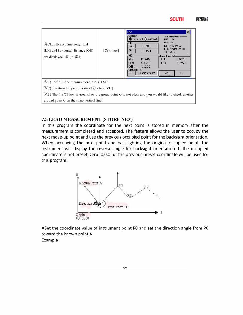
⑩Click [Next], line height LH
(LH) and horizontal distance (Off)
are displayed ※1)~※3)
[Continue]
※1) To finish the measurement, press [ESC].
※2) To return to operation step ⑦ click [VD].
※3) The NEXT key is used when the groud point G is not clear and you would like to check another
ground point G on the same vertical line.
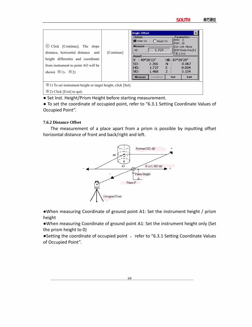
7.5 LEAD MEASUREMENT (STORE NEZ) In this program the coordinate for the next point is stored in memory after the measurement is completed and accepted. The feature allows the user to occupy the next move‐up point and use the previous occupied point for the backsight orientation. When occupying the next point and backsighting the original occupied point, the instrument will display the reverse angle for backsight orientation. If the occupied coordinate is not preset, zero (0,0,0) or the previous preset coordinate will be used for this program.
●Set the coordinate value of instrument point P0 and set the direction angle from P0 toward the known point A. Example:

60
OPERATIONAL STEPS KEY DISPLAY
①Click [Store].
[Store]
②Use stylus select “Store”
[Store]
③Click [Set] to reset instrument
height or prism height. After
setting, click [Enter].
[Set]
④Collimate target p1 prism which
the instrument moves. Click
[Measure] to start survey.
[Measure]

61
⑤Click [Continue] .
The coordinates of P1 displays at
the bottom of screen.
[Continue]
⑥Click [Store] .
Coordinate of P1 will be confirmed.
The display returns to main menu.
Power off and move instrument to
P1 (Prism P1move to P0 )
[Store]
⑦After the instrument is set up at
P1, power on and start coord
measurement. Select Store, use
stylus to choose “Recall”. Show as
the right graph. ※1)
⑧Collimate the former instrument
point P0, click [Set].
The coordinate at P1and direction
angle toward P0 is set. The display
returns to main menu.
⑨Repeat the steps ①~⑧,as
required.
※1) Click [Exit].

62
7.6 OFFSET MEASUREMENT (OFFSET) There are four offset measurement modes in the Offset Measurement. 1.Angle offset 2.Distance offset 3.Plane offset 4.Column offset 7.6.1 Angle Offset This mode is useful when it is difficult to set up the prism directly, for example at the centre of a tree. Place the prism at the same horizontal distance from the instrument as that of point A0 to measure .To measure the Coordinate of the centre position, operate the offset measurement after setting the instrument height/prism height. ●When measuring coordinates of ground point A1: Set the instrument height/prism height. ●When measuring coordinates of ground point A0: Set the instrument height only. (Set the prism height to 0)
●In the Angle Offset Measurement Mode, there are two setting methods for the vertical angle. 1.Free vertical angle :The vertical angle will be changed by rotating telescope. 2.Hold vertical angle :The vertical angle will be locked and never changed by rotating telescope. When sighting to A0, you can select one way, [Hold] is to fix vertical angle to the prism position. When you select [Free], SD (Slope Distance) and VD (Vertical Distance) will be changed according to the movement of telescope. Example:

63
OPERATIONAL STEPS KEY DISPLAY
① Click [Offset].
[Offset]
② In the prompted dialogue box
click [Angle Offset] to enter into
angle offset measurement.
③Use the stylus to select “Free
VA” (or “Fixed VA”) to start angle
offset measurement.
Angle
Offset
④ Collimate prism P , Click
[Measure] to start measurement.
Sight prism P
Measure
⑤Use horizontal clamp screw and
horizontal tangent to sight target
A0.
CollimateA0
64
⑥ Click [Continue], The slope
distance, horizontal distance and
height differentia and coordinate
from instrument to point AO will be
shown ※1),※2)
[Continue]
※1) To set instrument height or target height, click [Set].
※2) Click [Exit] to quit.
● Set Inst. Height/Prism Height before starting measurement. ● To set the coordinate of occupied point, refer to “6.3.1 Setting Coordinate Values of Occupied Point”. 7.6.2 Distance Offset
The measurement of a place apart from a prism is possible by inputting offset horizontal distance of front and back/right and left.
●When measuring Coordinate of ground point A1: Set the instrument height / prism height ●When measuring Coordinate of ground point A1: Set the instrument height only (Set the prism height to 0) ●Setting the coordinate of occupied point ,refer to “6.3.1 Setting Coordinate Values of Occupied Point”.

65
OPERATIONAL STEPS KEY DISPLAY
① In Offset dialog box, click
[Distance Offset] to enter into Dist.
Offset.
[Distance
Offset]
②Move stylus to “Input”, enter the
offset distance. When each value is
inputted, use stylus to move the
next item.
③After inputting “dRL”, sight the
prism, click [Measure] to start
measure.
[Measure]
④Click [Continue], the corrected
measure result displays, as shown
in the right picture. ※1),※2)
[Continue]
※1) To set instrument height or target height, click [Set].
※2) Click [Exit] to quit.
7.6.3 Column Offset If it is possible to measure circumscription point (P1) of column directly, the distance

66
to the center of the column (P0), coordinate and direction angle can be calculated by measured circumscription points (P2) and (P3). The direction angle of the center of the column is 1/2 of total direction angle of circumscription points (P2) and (P3)
●Setting the coordinate of occupied point ,refer to “6.3.1 Setting Coordinate Values of Occupied Point ”. Example:
OPERATIONAL STEPS KEY DISPLAY
① In Offset dialog box, click
[Column Offset] to enter into
Column Offset measurement.
[Column
Offset]
② Collimate the center of the
column (P1) and click [Measure] to
measure. After measuring, click
[Continue].
[Measure]

67
③Collimate the point (P2) on the
left side, as shown in the right
graph. Click [Continue].
[Continue]
④Collimate the right side of the
column (P3)
⑤Click [Continue], the distance
between the instrument and center
of the column (P0) will be
calculated and displayed ※1),※
2)
[Continue]
※1) To set instrument height or target height, click [Set].
※2) Click [Exit] to quit.
7.6.4 Plane Offset Measuring will be taken for the place where direct measuring can not be done. For example distance or coordinate measuring for an edge of a plane. Three random target points (P1, P2, P3) on a plane will be measured at first in the Plane Offset measurement to determine the measured plane. Collimate the target point (P0) then the instrument calculates and displays coordinate and distance value of cross point between collimation axis and of the plane.

68
●Setting the coordinate of occupied point, refer to “6.3.1 Setting Coordinate Values of Occupied Point”. Example:
OPERATIONAL STEPS KEY DISPLAY
①In Offset dialog box, click [Plane
Offset] to enter into Plane Offset
measurement.
[Plane Offset]
②Sight prism P1, click [Measure]
to start measure After measuring,
click [Continue].
[Measure]
[Continue]
③ Measure the points P2 ,
Click[Measure] to start measure..
After measuring, click [Continue].
[Measure]
[Continue]

69
④Sight prism P3,Click [Measure]
to start measure.
[Measure]
⑤Click [Continue] to calculate and
display coordinate and distance
value of cross point between
collimation axis and of the plane .
※1)
[Continue]
※1) To set instrument height or target height, click [Set].
●In case the calculation of plane was not successful by the measured three points, error displays. Start measuring over again from the first point. ●Error will be displayed when collimated to the direction which does not cross with the determined plane. 7.7 PARAMETERS SETTING In basic survey, some parameters can be set. Communication Parameters Factory default settings are indicated with underlines.
Menu Selecting Item Contents 1. Baud Rate 1200/ 2400/ 4800/
9600/19200/38400/57600
Select the baud rate
2. Data
Number
7 / 8 Select the data length seven digits or eight digits
3. Stop Bit 1 / 2 Select the stop bit.
4. Check Mode None/Odd/Even Select the parity bit.
5. ACK/NAK
Yes /No
When communicating to an external device, the protocol for
handshaking can omit the [ACK] coming from the external
device so data is not send again.
Yes:Omit the [ACK]
No :Standard

70
Other Parameters Menu Selecting Item Contents 1. Coord. Ranking NEZ/ENZ Select the display format in the coordinate
measurement mode for NEZ or ENZ
2.Occ Save 0 Set / Save Select whether to save coordinate of occupied
point or 0 Set.
3.Angle Unit Deg/Gon/Mil
Select degree (360°) , gon (400 G) or mil (6400
M) for the measuring angle unit to be shown on
the display
4.Dist Unit Meter/Int.Feet/U.S Feet Select the distance measuring unit.
Example:
OPERATIONAL STEPS KEY DISPLAY
① In the main menu of basic
survey, click [Para.] to enter into
Parameter Setting.
[Para.]
②Use stylus to select items.
③Click the “▼” beside “Baud”,
select the baudrate you need.

71
④ To use the default
communication parameters, click
[Default].
[Default]
⑤To set other parameters, click
[Other Parameter]. Set as the same
method.
[Other
Parameter]
⑥After setting click [OK] to quit.
The display returns to basic survey
main menu.
[OK]
8. START STANDARD SURVEY PROGRAM
In Total station main menu, click “ ” to enter standard survey program. The screen displays
as follows:

72
Main feature of standard survey program: ●Multiple Job Files Standard Survey Software uses named jobs with separate files for raw data, coordinates and strings. The job is given alphanumeric names. You may have many jobs in the system. You may create a new job for storing data, or you may open an existing job for data storage. You may also delete job files. ●Traverse & Topographic Recording Sequences Backsight and Foresight observation options allow user to record traverses or sets of multiple observations in any sequence. Multiple observations of foresights and backsights are averaged dynamically. A side shot option allows data collection for topographic surveys. Traverse and topographic collection may be combined. ●Offsets A single offset option is activated by a function key and allows manual entry of perpendicular offsets, or calculated offsets, including remote elevation from a second angle reading. ●Point Coordinate and String Generation Coordinates are generated in real‐time with optional storage. Stored coordinates are recalled at occupied stations and used for back bearing calculation. ●Horizontal Circle Setting Backsight bearing may be set on the instrument from calculated coordinates or manual input. ●Control point Coordinate Library Every control point library is accessible by all jobs for storage of frequently used coordinates. Control point file may be entered manually, or uploaded from computer. ●Point Code Library Point codes may be selected from the library file. ●Edit and Delete Data Raw data, point coordinates, control point coordinates and codes may be edited and deleted in the total station. ●Download to Serial Port Raw data, coordinates can be sent to a computer by using a serial cable.

73
●Upload Point Code from Serial Port The point code of total station may be created by uploading codes from a computer. ●Upload Roads Design data from serial port Horizontal alignment data, vertical alignment data and cross section data for Alignment lay out can be uploaded from serial port. ●Point Setting‐Out The standard setting out program calculates bearing and distance, displays offsets from occupied point to lay‐out point after each measurement. Coordinates of set‐out points can be saved and differences downloaded in the fill‐cut files. Note that the scale factor defined under the SETUP will be used in the calculation of setting out distances. ●Strings Setting Out Setting out of points by string (point code) allows the setting out of points on a line created in design software. ● Road Setting Out Two options allow the setting out of points by chainage and offset from a road alignment. Refer to Road Alignment. ●Traverse Adjustment The Bowditch adjustment method is used to adjust a recorded traverse. The traverse is defined by entering start and end points and the intermediate points are determined from foresight observations. ●Resection Computation of coordinates from known points. The method of calculation is dependent on the data available. Either two points with angles and distances, or three points with angles only are required. Where more than three points and up to maximum of 10 points are available the least squares method is used. Note that the scale factor defined under the SETUP function will be used is the calculation. ●Occupied Point Elevation Computation Computation of the occupied point elevation by single observation to a known point. ●Intersections

74
Coordinates calculation from two known points, with either bearings or distances. ●Inverse Computation of bearing and distance between 2 known points, Note that the scale factor defined under the MENU function will be used in the calculation of distances. ●Area Calculation Area calculation of a serial of points defined by point code. ●Radiation Coordinates of a point can be computed by entering bearing and distance. ●Missing Line measurement The slope distance, horizontal distance and vertical distance between two points can be computed. ●Batter boards A program for setting out in building area. If two points can not be setout, a batter board can be placed in the vicinity. The intersection point of the line connecting two setout points and the batter board can be found. ●Tape Dimension Tape dimension is a program which integrates surveying using a total station and a measuring tape. This program is especially useful when a quick survey of an object is required.
9. PROJECT In standard survey menu, click [Project].
This menu allows following functions be performed: (1) Create, open, delete job file (2) Setting job option

75
(3)Set scale factor (4) Data export/import Standard measuring program require that every time measuring you must create a job file name, if not, system will create a default file name (default) automatically. All the measuring results will be saved in this file. 9.1 CREATE NEW PROJECT Create a new project file. A job name has a maximum of 16 characters and should be made up from the letters A‐Z, numbers 0‐9 and the minus sign (_# $ @ % + ‐), but the first character can not be a space.
OPERATIONAL STEPS KEY DISPLAY
① In [Project] menu, click
[New].
[New]
②In the prompt dialog box, enter
name of project, operator, and brief
information. After inputting one
item, use stylus to click the next
item. ※1)
Enter
information
③Inputting all, click [Create] to
save. The new created project is
defaulted as current project. The
system return to standard survey
main menu. ※2),※3)
[Create]
※1)Project:All the measurement data will be stored in this file.
Operator:Operator’s name (Can be default).
Brief:Brief information of the project. (Can be default)
Other:The operator can enter other information, such as instrument model.( Can be default)

76
※2) Press [ESC] key to exit the screen without saving the settings.
※3) If the project exists, the system prompts “Project are the same!” So, select OPEN option to see a
list of current jobs before creating the new job if you are not sure which jobs currently exist.
9.2 OPEN PROJECT Example:
OPERATIONAL STEPS KEY DISPLAY
①In [Project] menu,,Click [Open]
or press [▲]/[▼] to select. The
screen lists all jobs in internal
memory.
[Open]
②Double click to open the project,
or input project name in the Name
field.
③In the prompt dialog box, double
click project name to open the
project. All the measurement data
will be stored in this file. The
display returns to standard survey
main menu.
※1)
※1) Press [ESC] to quit and return to last screen standard survey main menu.
9.3 DELETE PROJECT Example:

77
OPERATIONAL STEPS KEY DISPLAY
① In [Project] menu, , Click
[Delete] or press [▲]/[▼] to select.
The screen shows as the right
graph.
[Delete]
②Double click the project you
want to delete.
The system defaults to delete all
projects. To delete some data of the
project, click “Delete Files” and
then choose the data files need to
delete in the File Option. ※1)
Delete some files:
③ Click [Delete]. The system
prompts Delete successful!”※2)~
※3)
[Delete]
※1)Delete all project:Delete all content of the selected job.
※2) Current project can’t be deleted.
※3) Click [Browse] to view project in internal memory.

78
9.4 OPTION OPERATIONAL STEPS KEY DISPLAY
①In [Project] menu, , Click
[Option] (or press [▲]/[▼] to
select), the screens as the right
graph.
[Option]
②Click each item to set. Click [Set]
to return.
[Set]
Options: Fixed File:Set fixed point file [On] or [Off]. 1)If it is set as [On], when the fixed point file will be scanned for coordinates before prompting for the coordinates. When the same point number is saved in coordinate database or fixed database. The data in [coordinate data] will be called up. 2)If the station file option is OFF, the fixed point file is not searched. Coord. Display:Set whether to display coordinate of NEZ during measurement. Coord Transform:Set whether to calculate and save coordinate. 1)If set as [On], when the measuring mode is H/V/SD or H/HD/VD, the coordinates will be calculated and saved automatically. 2)If set as [Off], the calculated coordinate will not be saved. [Note]:In adjusting traverse, to save coordinate or set the calculated bearing angle into instrument, this option should be set to ON. Layout Save:The setting of storing layout point coordinates. When the coordinates are saved, each layout point with designed coordinates and layout coordinates and cut or fill height will be listed. ※Note that System Setting apply to all jobs, when it is changed, all jobs will be affected.

79
9.5 GRID FACTOR Measured horizontal distance is multiplied by the scale factor in coordinate calculation. The raw data is not altered by the scale factor. Enter the scale factor and the mean elevation into screen, the downloaded raw data will contain a scale factor record. The following grid factor is used to calculate coordinates. Calculation Formula
1. HEIGHT FACTOR= ELEVRR
+
R : The average radius of the earth ELEV:The height of the mean sea level 2. SCALE FACTOR Scale factor: the scale on the measurement station GRID FACTOR Grid factor = height factor×scale factor Distance Calculation 1. GRID DISTANCE HDg = HD × Grid factor HDg:Grid distance HD :Ground distance 2. GROUND DISTANCE
HD =GridHDg
Enter the scale factor and elevation. Example:
OPERATIONAL STEPS KEY DISPLAY
①In [Project] menu,,Click [Grid
Factor]( or press [▲]/[▼] to
select),the screen displays as the
right graph.
[Grid Factor]

80
②Input the Scale and Elevation.
③The system calculates the grid
factor. Click [Enter].The display
returns to standard survey main
menu.
[Enter]
Note:1. Inputting range of scale:0.990000 ~ 1.010000. The default value: 1.00000 2. Inputting range of average altitude: -9999 ~ 9999 The default value: 0
10. DATA EXPORT/IMPORT 10.1 DATA EXPORT Measuring data coordinate and data of dig/fill, cross section may be downloaded to a computer.
OPERATIONAL STEPS KEY DISPLAY
① In project menu, click [Data
Export].
[Data Export]

81
②In the prompt dialog, click the
data you want to export. Click
[Export].
[Export]
③Select the place to save export
data Input file name in the Name
field.
④Click [OK], then data is export
to appointed position. And the
display returns to standard survey
main menus.
[OK]
USB HDD Export: 960 allow surveyer move data through function of USB transmission. Export the data you need to the disk inside of the total station first. System will save the result in TXT form..Plug in the USB HDD,then you could find that icon of USB HDD in 960 system.Copy that file you need to USB HDD and disconnect it from total station.At least,you could move that data file to your PC easily. SOFTWARE EXPORT Export the project you need to the disk inside of the total station first. System will save the result in TXT form. Then connect the 960 total sation to computer with the USB cable after checking that if there Microsoft ActiveSync software has already been installed. Microsoft ActiveSync will show as follow:

82
At same time this icon will appear in your My computer.
Now you should find the TXT form file in Mobile Device and copy them to your pesonal PC disk.The process is completed. 10.2 DATA IMPORT Coordinate files for set out, fixed point and code library files, alignments and cross section files for set out may be uploaded from a computer to the total station by series port. Example:
OPERATIONAL STEPS KEY DISPLAY
① In Project menu, click [Data
Import].
[Data Import]

83
②Select the data type you need to
import, and click [Import]. ※1)
[Import]
③The imported file is found.
④Click [OK], data is imported to
appointed position and return to
standard survey main menu.
[OK]
※1)HZ Alignment:Upload a horizontal alignment for road design layout. Data format please refer to
appendix A. There is only one start point can be existed in a block of horizontal alignment data;
otherwise it may cause some mistakes.
VT Alignment:Upload a vertical alignment for road alignment layout. Data format is described in
Appendix A.
X-Sect Data:upload a design cross section file for road design layout:The uploaded cross sections
cannot be edited nor downloaded. Data format is described in Appendix A.
USB HDD Import: Make sure that the TXT form data you need to transmit has already existed in USB HDD. Plug in the USB HDD,then you could find that icon of USB HDD in 960 system.Find out the TXT form file you want to transmit.Use copy or cut moving function to transmit the TXT form file to 960 system,Open the Standared survey program and import the TXT file you just copy from PC.This process is completed.

84
SOFTWARE IMPORT: Connect the 960 total sation to computer with the USB cable after checking that if there Microsoft ActiveSync software has already been installed. Microsoft ActiveSync will show as follow:
Find out the TXT form file you want to transmit.Use copy or cut moving function of windows to transmit the TXT form file to Mobile Device, the icon of which shown as:
After that you could find that file in the Total station’s disk.Open the Standared survey program and import the TXT file you just copy from PC.This process is completed.
11. RECORD MEASUREMENT DATA The RECORD menu is mainly used for collecting and recording raw data. It allows setting occupied point and backsight bearing, start backsight observation, foresight observation, sideshot observation and cross section observation. In standard survey main menu, click [Record] or press [ ]/ [ ].

85
11.1 SETTING OCCUPIED POINT AND BACKSIGHT POINT Example:
OPERATIONAL STEPS KEY DISPLAY
①In [Record] menu, click [Setup]
※1)
[Set]
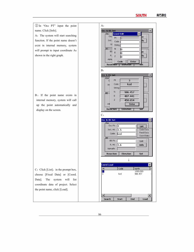
86
② In “Occ PT” input the point
name. Click [Info].
A:The system will start searching
function. If the point name doesn’t
exist in internal memory, system
will prompt to input coordinate As
shown in the right graph.
B: If the point name exists in
internal memory, system will call
up the point automatically and
display on the screen.
C:Click [List],in the prompt box,
choose [Fixed Data] or [Coord.
Data]. The system will list
coordinate data of project. Select
the point name, click [Load].
A:
B:
C:
↓

87
③Input the backsight point.
④ The system calculates the
azimuth.
⑤Click [Set] to enter into BS Set
function.
Bks:Bearing calculated by system
or entered manually.
HR:Current horizontal azimuth.
[Set]

88
⑥ A : If click [0 Set] , then the
horizontal angle displays 0.
Click [Enter] to quit and set BS
azimuth as 0.
B:If click [Set], the HR displays as
the azimuth.
C:
If click [Check], backsight point
coordinate will be checked by
measuring the slope distance of
backsight point.
D:
If click [Enter], the current
horizontal angle is recorded as the
initial backsight direction, and use
for coordinate calculation.
A:
B:
C:
⑦Click [Enter] to finish setting BS
point and return to standard survey
main menu.
[Enter]
※1) Resection: The resection function key which is used to calculate the occupied point coordinate.
Elevation:The function key for measuring the elevation of a point
Details see “11.1.1Resection” and “11.1.2Elevation of Occupied Point”
※Note:If the point exists both in the point file and fixed point file, then coordinates from the point file will be used. 11.1.1 Resection If the coordinates of an occupied point are unknown, a resection can be performed to

89
compute these coordinates. A resection involves the measurements from an occupied point to several other points with known coordinates. It is possible to perform a resection by measuring angles and distances or by measuring angles only. The type of measurements influences the minimum number of observations needed to perform a resection. In case of angle as well as distance measurements a minimum of 2 observations are required, by measuring angles only a minimum of 3 observations should be performed.
OPERATIONAL STEPS KEY DISPLAY
①In [Occ. & BS Set] menu input
occupied point name, click
[Resection]. If the point name
doesn’t exist in internal memory,
system will prompt to input
coordinate After saving the data,
click [Resection].
[Resection]
② Click [Add] to add a new
resection measurement. As shown
in the right graph.
[Add]

90
③Input the number of know point
which used for resection and prism
height.
Input PT,
prism height
④Click [Mode] to choose measure
mode.
[Mode]
⑤Sight the center of target prism,
click [Measure] to start measure.
[Measure]
⑥After measuring, click [Record],
a dialog box shows as the right
graph. Click [OK] to record the data
to the project.
[Record]

91
⑦The system returns to resection
main menu. The screen displays the
PT just measured If the coordinate
is unknown, system will request
user to input the coordinates and
then return to resection main menu.
⑧Click [Add] again, repeat steps
②~⑥ to finish measuring and
recording other resection points.※
1)
[Add]
⑨In case 3 angle measurements or
2 angle and distance measurements
have been performed, the
coordinates of the occupied point
can be displayed by pressing
[Coord]. Click [Enter].※2)
※1 )On the lower side of the screen discrepancies (e1) or the standard deviation in N, E, Z direction
(sN, sE, sZ) of the occupied point will be displayed. Discrepancies will be shown in case two distance
measurements have been performed. They are calculated using the following equations.
e1 = HD12 (Calculated using measurements) – HD12 (Calculated using known coordinates)
HD12 denotes the horizontal distance between the first and second point.
※2) If the distance of more than three points or angles of more than four points have been measured;
the standard deviation will be displayed instead of discrepancies. The number of residuals shown
depends on the parameters selected. Generally, the worst observation will have the largest residual. This
observation can be deleted by placing the bar on this observation using the arrow key and then press
[DEL]. The observation is removed from the list. The coordinates of the occupied point, its standard
deviation or discrepancies and the residuals of the remaining observations are automatically
recomputed.
By clicking [Para.], the parameters which are calculated during resection can be selected. The following screen will be shown.

92
●It is possible to select whether the level of the occupied point, a scale factor or the backsight bearing (‘Calculate Bkb’) should be calculated. Furthermore it is possible to select whether the calculated scale or the measurements which have been performed (‘Store res meas’) should be stored. ● After setting, click [Enter] to return to the main resection screen, saving the changed mode and (re)calculation of the occupied point, residuals and the required parameters.
Press [ENT] in the resection main menu will quit this function and save the coordinates of the occupied point. In case ‘Store res meas’ was turned on in [PARAM], the measurements which have been performed and which are shown in the box will be saved as well.
In case ‘Calculate Bkb’ in [PARAM] was turned on, the backsight bearing will be calculated and set by pressing [ENT] key and leaving the main resection screen. The computation will use all measurements which are shown in the box. In order to calculate a backsight bearing of high quality: The residuals of the horizontal angle should have low values. The user shouldn’t change the horizontal angle when leaving the main resection screen. NOTE : 1) The measurements can be performed in any order. The point numbers shown in the box in the main resection screen will be sorted by horizontal angle. 2) When 3 points are used for resection using angle measurement only, you must
consider the “danger circle.”
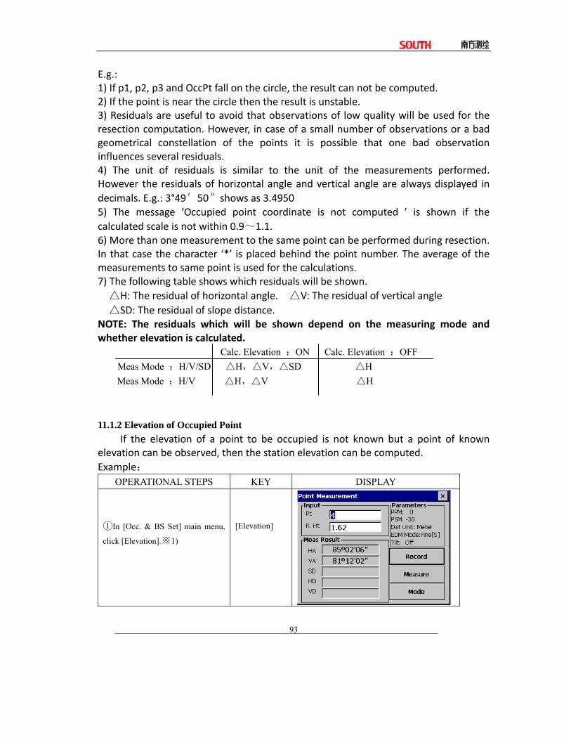
93
E.g.: 1) If p1, p2, p3 and OccPt fall on the circle, the result can not be computed. 2) If the point is near the circle then the result is unstable. 3) Residuals are useful to avoid that observations of low quality will be used for the resection computation. However, in case of a small number of observations or a bad geometrical constellation of the points it is possible that one bad observation influences several residuals. 4) The unit of residuals is similar to the unit of the measurements performed. However the residuals of horizontal angle and vertical angle are always displayed in decimals. E.g.: 3°49′50″shows as 3.4950 5) The message ‘Occupied point coordinate is not computed ’ is shown if the calculated scale is not within 0.9~1.1. 6) More than one measurement to the same point can be performed during resection. In that case the character ‘*’ is placed behind the point number. The average of the measurements to same point is used for the calculations. 7) The following table shows which residuals will be shown. △H: The residual of horizontal angle. △V: The residual of vertical angle △SD: The residual of slope distance. NOTE: The residuals which will be shown depend on the measuring mode and whether elevation is calculated. Calc. Elevation :ON Calc. Elevation :OFF Meas Mode :H/V/SD △H,△V,△SD △H
Meas Mode :H/V △H,△V △H 11.1.2 Elevation of Occupied Point If the elevation of a point to be occupied is not known but a point of known elevation can be observed, then the station elevation can be computed. Example:
OPERATIONAL STEPS KEY DISPLAY
①In [Occ. & BS Set] main menu,
click [Elevation].※1)
[Elevation]
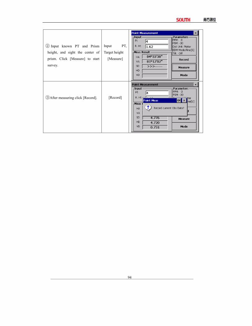
94
② Input known PT and Prism
height, and sight the center of
prism. Click [Measure] to start
survey.
Input PT,
Target height
[Measure]
③After measuring click [Record].
[Record]

95
④Click [OK].
A:If the point name doesn’t exist in
internal memory, system will
prompt to input coordinate As
shown in the right graph. System
calculates height of occupied point
automatically.
B:If the coordinate of the point
exists in the file, System calculates
height of occupied point
automatically.
[OK]
A:
↓
↓
B:
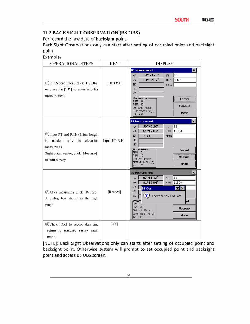
96
11.2 BACKSIGHT OBSERVATION (BS OBS) For record the raw data of backsight point. Back Sight Observations only can start after setting of occupied point and backsight point. Example:
OPERATIONAL STEPS KEY DISPLAY
①In [Record] menu click [BS Obs]
or press [▲]/[▼] to enter into BS
measurement
[BS Obs]
②Input PT and R.Ht (Prism height
is needed only in elevation
measuring).
Sight prism center, click [Measure]
to start survey.
Input PT, R.Ht.
③After measuring click [Record].
A dialog box shows as the right
graph.
[Record]
④Click [OK] to record data and
return to standard survey main
menu.
[OK]
[NOTE]: Back Sight Observations only can starts after setting of occupied point and backsight point. Otherwise system will prompt to set occupied point and backsight point and access BS OBS screen.

97
11.3 FORESIGHT OBSERVATION (FS OBS) The data of Foresight Observations mainly used for the traverse adjustment calculation. After setting Occ point and BS point, the measuring begins. Example:
OPERATIONAL STEPS KEY DISPLAY
①In [Record] menu click [FS Obs]
or press [▲]/ [▼] to enter into FS
measurement.
[FS Obs]
②Input PT, R.Ht . 1)※ , 2)※
Input PT, R.Ht
③Input code, or click [Code] to call
up from code list. System lists
stored codes. Click the “+” before
the needed code layer. Double click
the needed code.
④System prompts the dialog box.
Click [OK] to select the code and
return to measure screen.
[OK]
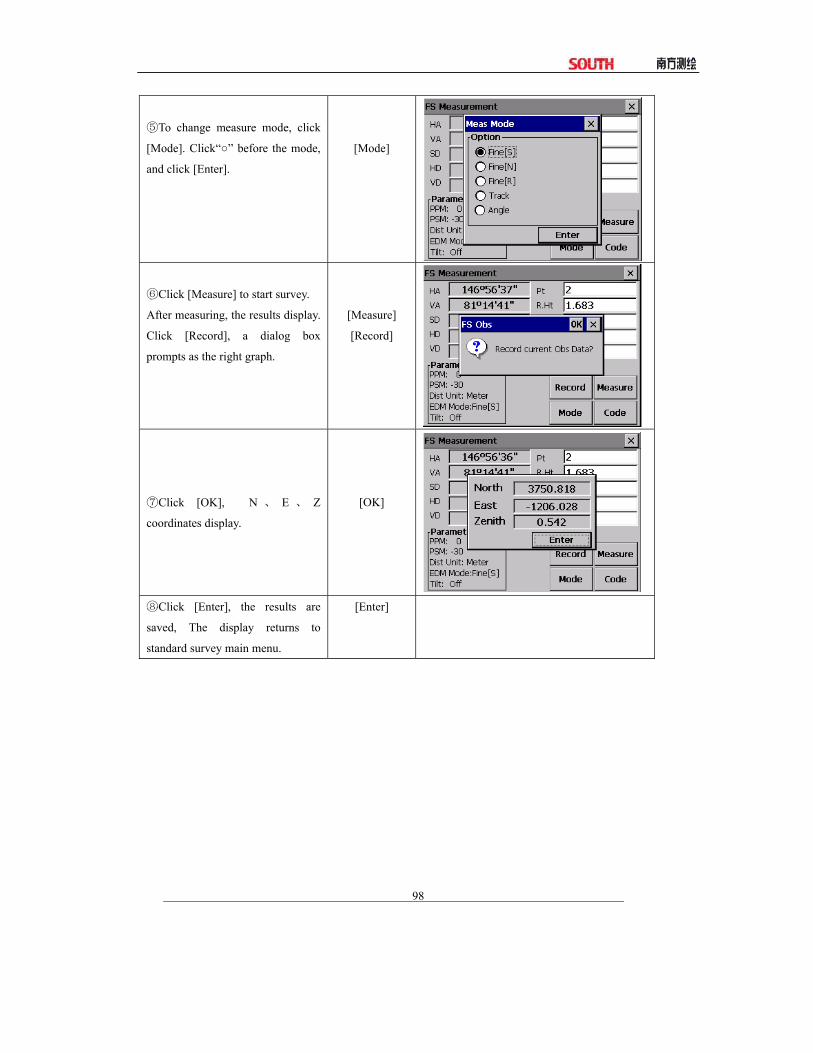
98
⑤To change measure mode, click
[Mode]. Click“○” before the mode,
and click [Enter].
[Mode]
Click⑥ [Measure] to start survey.
After measuring, the results display.
Click [Record], a dialog box
prompts as the right graph.
[Measure]
[Record]
Click⑦ [OK], N 、 E 、 Z
coordinates display.
[OK]
Click⑧ [Enter], the results are
saved, The display returns to
standard survey main menu.
[Enter]
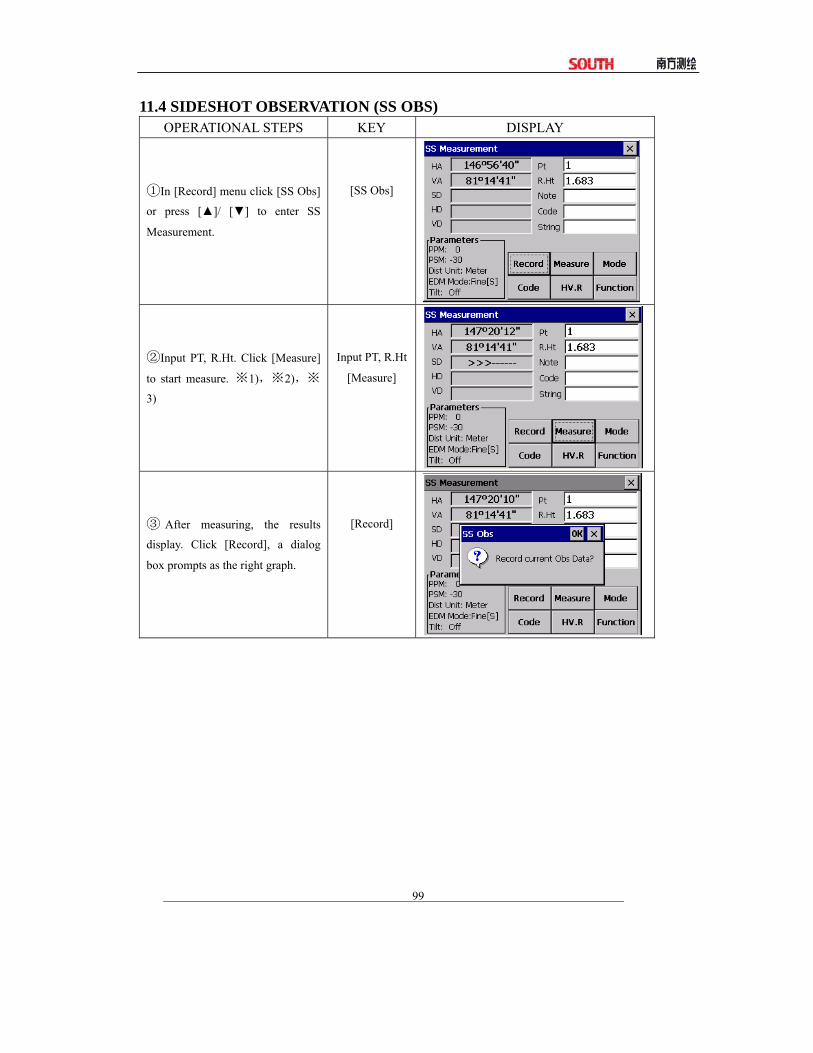
99
11.4 SIDESHOT OBSERVATION (SS OBS) OPERATIONAL STEPS KEY DISPLAY
①In [Record] menu click [SS Obs]
or press [▲]/ [▼] to enter SS
Measurement.
[SS Obs]
②Input PT, R.Ht. Click [Measure]
to start measure. ※1),※2),※
3)
Input PT, R.Ht
[Measure]
③ After measuring, the results
display. Click [Record], a dialog
box prompts as the right graph.
[Record]

100
④Click [OK], N、E、Z coordinates
display.
If the point exists, system prompts
whether to cover the point.
[OK]
⑤Click [Enter],the measurement
results are saved.
Repeat ② ~ ⑤ to finish
measurement.
[Enter]
※1) Click [Mode], to select measure mode among Fine[S]/Fine [N]/ Fine[R]/Track/Angle Meas.
※2) Click [Code] to call up code from code list.
※3)HV.R:Function used to record raw angle data.
FUNCTION KEY In [SS Obs], click [Function], the function menu prompts.

101
11.4.1 Offset Apply the following procedure to a point which can not be measured directly. Measured data change to raw data directly.
. A radial (forward) offset is along the line of sight, with positive away from the
instrument, and a tangential (right) offset is perpendicular to the line of sight with positive to the right, as viewed from the instrument. A vertical offset is positive upwards.
●Offsets may be entered manually if measured by tape, or computed by measuring a second angle to the required point.
A tangential offset may be computed by recording a second angle to intersect with the perpendicular offset from the current observation. This method can be used to obtain an approximate position for the center of an object, for example a tree. Take a shot to the side of the object. When the offset screen has been selected, sight the center of the object, and press [Horizon] to read the horizontal angle. A perpendicular offset from the original line of sight will be computed and entered to the screen.
To compute a vertical offset (remote elevation), make an observation to an accessible point above or below the point required. When in the offset screen, sight the point required, and press [Vertical]. The vertical angle will be used to compute the difference in elevation from the ground to the point above or below. The offset will be written to the screen. Make the current target height has been entered into the point code screen before selecting [Offset].

102
Record an observation as close as possible to the required point. OPERATIONAL STEPS KEY DISPLAY
①In [SS] function sight the prism
center. Click [Measure] to start
measure.
[Measure]
②Keep the instrument still, click
[Function]. A dialog box prompts as
the right graph.
[Function]
③In Function menu, click [Offset]
to enter Offset measurement.
[Offset]
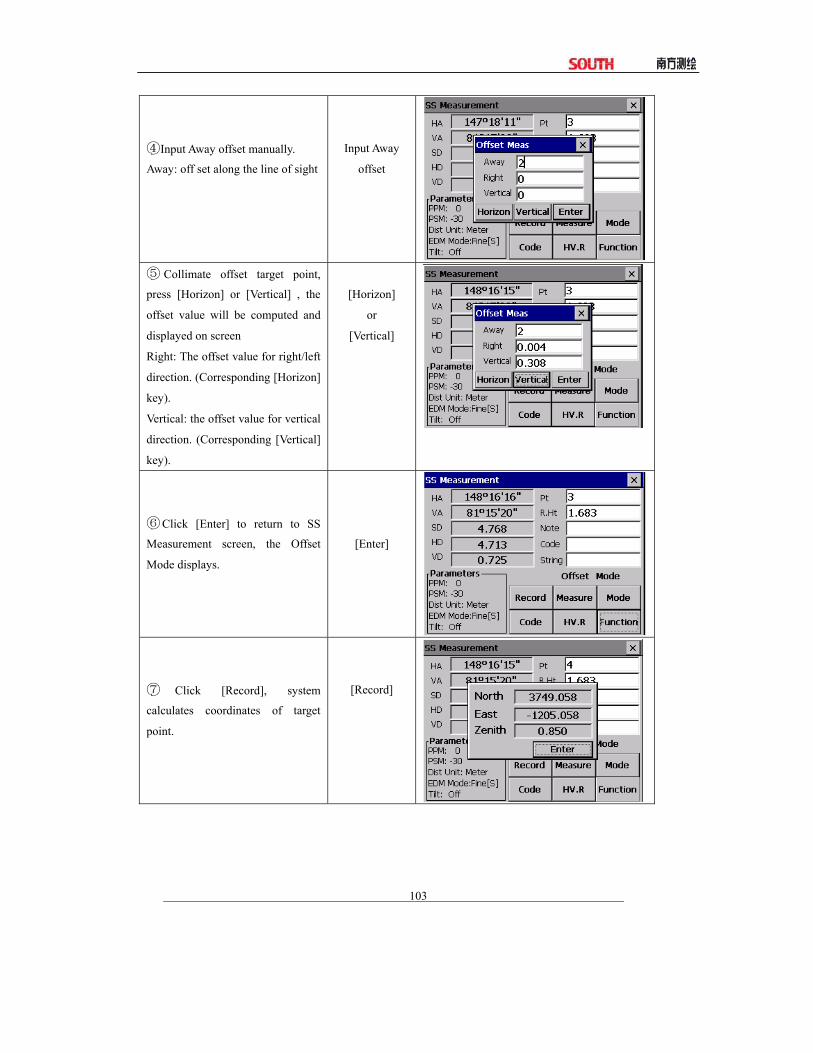
103
④Input Away offset manually.
Away: off set along the line of sight
Input Away
offset
⑤ Collimate offset target point,
press [Horizon] or [Vertical] , the
offset value will be computed and
displayed on screen
Right: The offset value for right/left
direction. (Corresponding [Horizon]
key).
Vertical: the offset value for vertical
direction. (Corresponding [Vertical]
key).
[Horizon]
or
[Vertical]
⑥Click [Enter] to return to SS
Measurement screen, the Offset
Mode displays.
[Enter]
⑦ Click [Record], system
calculates coordinates of target
point.
[Record]

104
⑧Click [Enter] to return to SS
Measurement screen.
[Enter]
11.4.2 Plane Offset This mode is similar with【PROGRAM】→【Offset】→【Plane Offset】. Example:
OPERATIONAL STEPS KEY DISPLAY
① In SS Measurement, click
[Function].
[Function]
②Click [Plane Offset] to enter into
Plane Offset Measure.
Click [Define], to enter into Define
Plane function. Click [Off] to return
to SS Measurement.
[Plane Offset]
③Sight the first point of the plane,
click [Measure] to start measure.
[Measure]
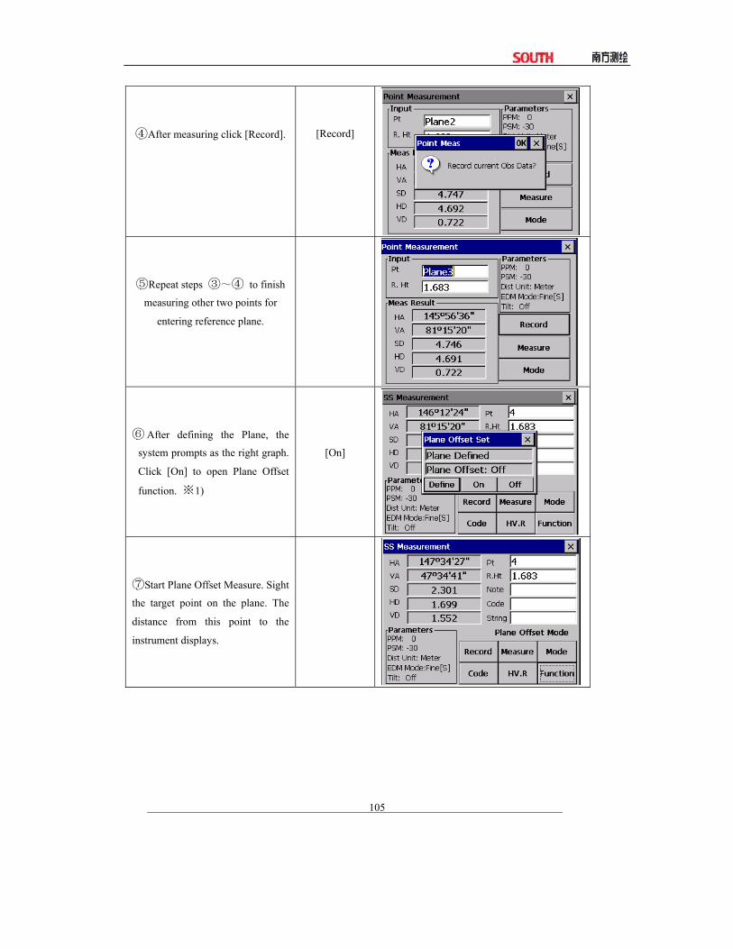
105
④After measuring click [Record].
[Record]
⑤Repeat steps ③~④ to finish
measuring other two points for
entering reference plane.
⑥After defining the Plane, the
system prompts as the right graph.
Click [On] to open Plane Offset
function. ※1)
[On]
⑦Start Plane Offset Measure. Sight
the target point on the plane. The
distance from this point to the
instrument displays.

106
⑧Click [Record] to record results
of Plane Offset.
[Record]
⑨Click [Enter] to save measuring
results.
Repeat steps ⑦~⑧ to finish
measuring other points on the
plane.
[Enter]
※1) [On]:Function key used to display “Plane Offset”. In SS Measurement screen “Plane Offset
Mode” shows
[Off]:Function key used to shut “Plane Offset”.
11.4.3 Pt. Line Mode (For Measurement from Point to Line) This mode is used for coordinate measurement of target points which treats A (0,0,0) as the origin and line AB as the N axis. See below:
A: reference point 1 B: reference point 2
●After measuring coordinates of point A, B, enter Point & Line Measurement Mode. Set A, B as reference point 1, 2. Set once again a coordinate system which has A as origin and line AB as N axis. Start measurement again. (Never change information of

107
occupied point during the process.) Example:
OPERATIONAL STEPS KEY DISPLAY
①Measure coordinates of Point A、
B,record in the memory. In SS
Measurement, click [Pt. Line
Mode] to enter into Point Line
Mode.
[Pt. Line
Mode]
②Define base line. Enter the Point
number of start point and stop point
If the point does not exist, it
displays “Coord PT not found!”
Press [Enter].
③After defining base line click
[On] to enter into Pt. Line measure
Mode.※1)
[On]
④ Sight prism center, click
[Measure] to start measure.
[Measure]

108
⑤After measuring click [Record].
[Record]
⑥Click[OK] to display coordinate.
[OK]
⑦Click [Enter] to save the results..
Repeat steps ④~⑥ to finish
measuring other points.
[Enter]
※1)[On]:It is used to activate Point to Line Mode.
[Off]:It is used to disable the Point to Line Mode.
11.4.4 Control Input Control Input function is used for editing the string and appended code of the point Example:

109
OPERATIONAL STEPS KEY DISPLAY
① In SS Measurement, Click
[CTRL Input] to enter into control
code Input function.
[CTRL Input]
②Input Control code, Code2 and
String 2. To call up code in code lib,
click [Code].
Input message
③Click [Enter], the screen returns
to SS Measurement screen.
11.5 CROSS SECTION SURVEY
The cross section survey allows points on a cross section to be surveyed and downloaded in chainage, offset and level format.
It operates similar to the side shot observation. Every cross section must have a center line point to compute the chainage and offsets.
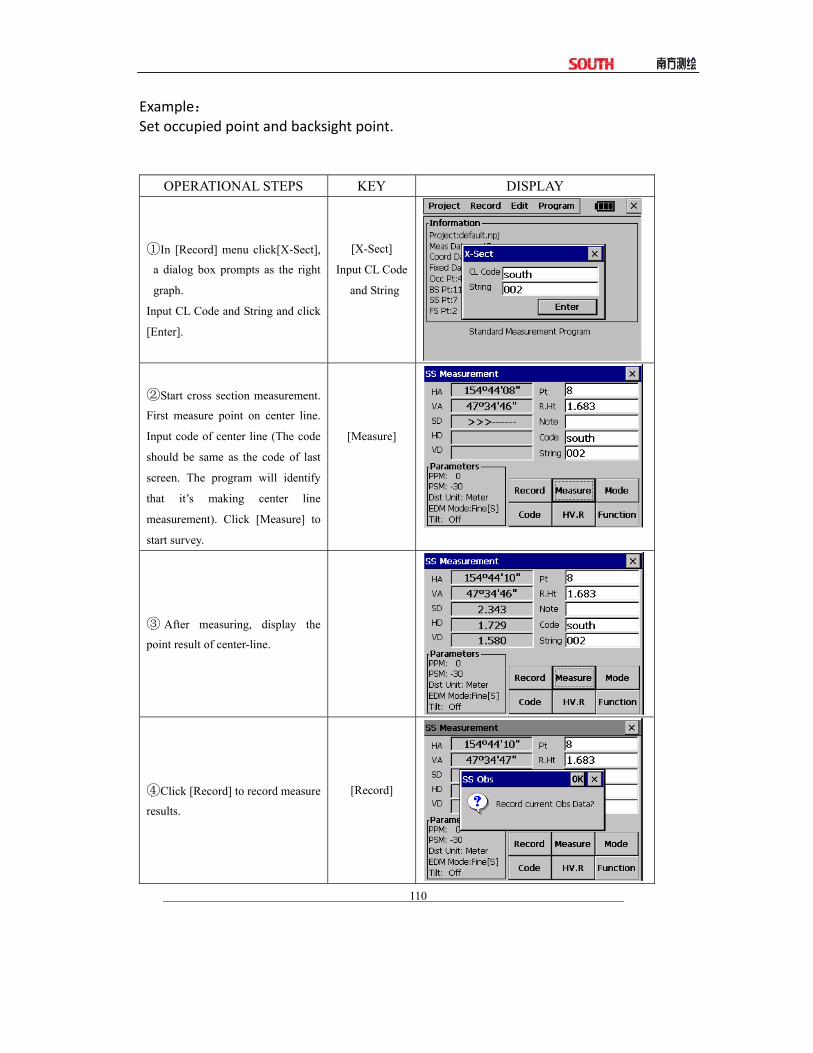
110
Example: Set occupied point and backsight point.
OPERATIONAL STEPS KEY DISPLAY
①In [Record] menu click[X-Sect],
a dialog box prompts as the right
graph.
Input CL Code and String and click
[Enter].
[X-Sect]
Input CL Code
and String
②Start cross section measurement.
First measure point on center line.
Input code of center line (The code
should be same as the code of last
screen. The program will identify
that it’s making center line
measurement). Click [Measure] to
start survey.
[Measure]
③ After measuring, display the
point result of center-line.
④Click [Record] to record measure
results.
[Record]

111
⑤ Click [OK] to display the
coordinates of this point. Click
[Enter] to save the results.
[OK]
[Enter]
⑥The screen returns to standard
measurement. Input code of each
point on the cross section, repeat
steps ②~⑤ to finish measuring
other points of this chainage and
save the result.
⑦After collecting all cross section
points of this chainage, click in SS Measurement, and a dialog box
prompt as the right graph. Input the
chainage of the cross section.(The
first chainage number must be input
by hand, the following chainages
can be calculated.)
⑧When the cross section is saved;
the screen will display the code of
mid-line and string. Click[Enter] to
receive the same code or enter new
code.
Click “ ” to quit X-Sect measurement record.
[Enter]

112
⑨Repeat steps ②~⑧ to finish
measuring points of cross section
on other chainages.
[NOTE]: (1.) The maximum point number for each cross section is 60. (2.) The chainage number automatically displayed is calculated as the horizontal distance from its occupied point to its center.
12. EDIT DATA The edit menu provides options to edit raw data, point coordinates, the fixed point library, and the code library.

113
12.1 EDITING RAW DATA To edit the raw data from the current job select Raw Data from the Edit menu.:
Function keys at the bottom of the screen: [Start]:Go to the beginning of this file. [End]:Return to the end of the file [Search]:To search a specific point, code or string in the file Example
OPERATIONAL STEPS KEY DISPLAY
①In Edit menu, click [Raw Data],
the system lists all measurement
data of the project.
[Raw Data]
②Find the needed data.
A: Click the slide bar to view all
data. Click the needed point name
when it appears. You can press
[▲]/[▼] to display the data.
A:

114
B:
Click [Search], in the prompt dialog
box input PT, Code, String, and
select between Full Name and Part
Name. Click [Search] to start
search.
B:
③After finding the needed data,
click [Edit],the Meas. Data Edit
dialog box appears.
[Edit]
④Input new data, and then click
[Save],system returns to last screen.
※1),※2)
[Save]
※1) Date, time and measure data can’t be modified.
※2) Press [ESC] to return to standard survey main menu.
NOTE:1. The range of each coordinate is from ‐9999999.999 to 9999999.999 2. Coordinates that are entered or changed are rounded to 3 decimal places.

115
12.2 COORD. DATA The coordinates generated from the current job may be edited or point coordinates may be manually entered. In [Edit] menu click [Coord. Data].
12.2.1 Edit Coord. Data Example:
OPERATIONAL STEPS KEY DISPLAY
① In Edit Menu, click [Coord.
Data], system lists all coord. data
in the project.
[Coord. Data]

116
②Search the needed coord. data
A:Click the slide bar to display all
coord. data. Click the needed point
name when it appears. You can
press [▲]/[▼] to view the data.
B:
Click [Search], in the prompt dialog
box input PT, Code, String, and
select between Full Name and Part
Name. Click [Search] to start
search.
A:
B:
③After finding the needed data,
click [Edit], the Coord. Data Edit
dialog box appears.
③Click [Edit], the dialog box of
this point coordinates prompts.
[Edit]
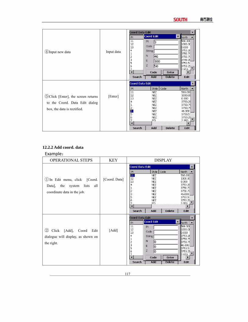
117
④Input new data
Input data
⑤Click [Enter], the screen returns
to the Coord. Data Edit dialog
box, the data is rectified.
[Enter]
12.2.2 Add coord. data Example:
OPERATIONAL STEPS KEY DISPLAY
① In Edit menu, click [Coord.
Data], the system lists all
coordinate data in the job.
[Coord. Data]
② Click [Add], Coord Edit
dialogue will display, as shown on
the right.
[Add]

118
③ Input PT ID, Code, String, and
N, E, Z coordinate.
Input PT ID,
Code, String,
and
coordinate.
④ Click [Enter], and return to
previous screen. The data will be
added on the bottom of the
profiles.
[Enter]
12.2.3 Delete Coord. Data Example:
OPERATIONAL STEPS KEY DISPLAY
① Find the data to be deleted with
the method mentioned previously.
② Click [Del], a notice is
displayed, as shown on the right.
[Del]

119
③Click [OK] and the data are
deleted. The screen returns, and
the cursor moves to next row.
[OK]
NOTE:1. The range of each coordinate is from -9999999.999 to 9999999.999
2. Coordinates that are entered or changed are rounded to 3 decimal places.
12.3 FIXED POINT DATA To edit the fixed point library select Fixed Data from the EDIT menu. This function is used to edit the coordinates of control point. Editing the fixed point data is similar to editing Coord.Data in the EDIT menu. 12.4 CODE DATA To edit the code library select Code Lib from the EDIT menu.
[Delete]:Delete a layer. [Edit]:Rename a layer. [Add]:Add a layer.
12.4.1 Create New Layer Example:

120
OPERATIONAL STEPS KEY DISPLAY
① In Edit Menu, click [Code
Data], the system lists all code
data in the job.
[Code Data]
②Click [Add] to display a dialogue
as shown on the right. Input Layer,
Code and Attribute in the
dialogue.
[Add]
③ A:
To input new code on an existed
layer, just input the code and
attribute.
B:
To add a layer, input the new layer,
code, and attribute.
A:
B:

121
④ A:
New codes are added under the
layer.
B:
A new code layer and code will be
created.
A:
B:
12.4.2 Edit Layer/Code
OPERATIONAL STEPS KEY DISPLAY ①Use the stylus to click on the
layer or code to be edited.
A:Layer
B:Code
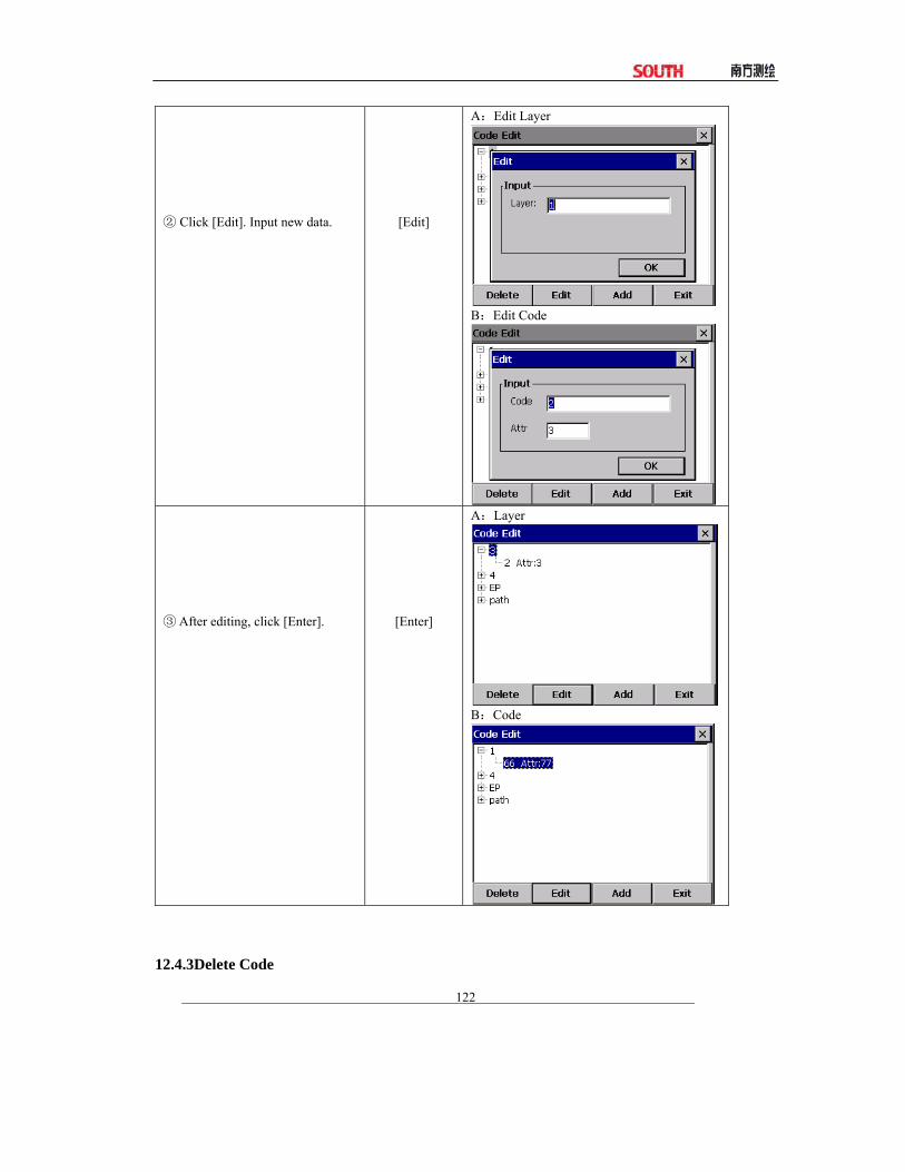
122
② Click [Edit]. Input new data.
[Edit]
A:Edit Layer
B:Edit Code
③ After editing, click [Enter].
[Enter]
A:Layer
B:Code
12.4.3Delete Code
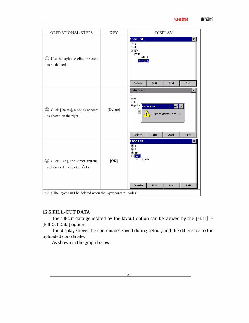
123
OPERATIONAL STEPS KEY DISPLAY
① Use the stylus to click the code
to be deleted.
② Click [Delete], a notice appears
as shown on the right.
[Delete]
③ Click [OK], the screen returns,
and the code is deleted.※1)
[OK]
※1) The layer can’t be deleted when the layer contains codes.
12.5 FILL-CUT DATA The fill‐cut data generated by the layout option can be viewed by the [EDIT]→
[Fill‐Cut Data] option. The display shows the coordinates saved during setout, and the difference to the
uploaded coordinate. As shown in the graph below:
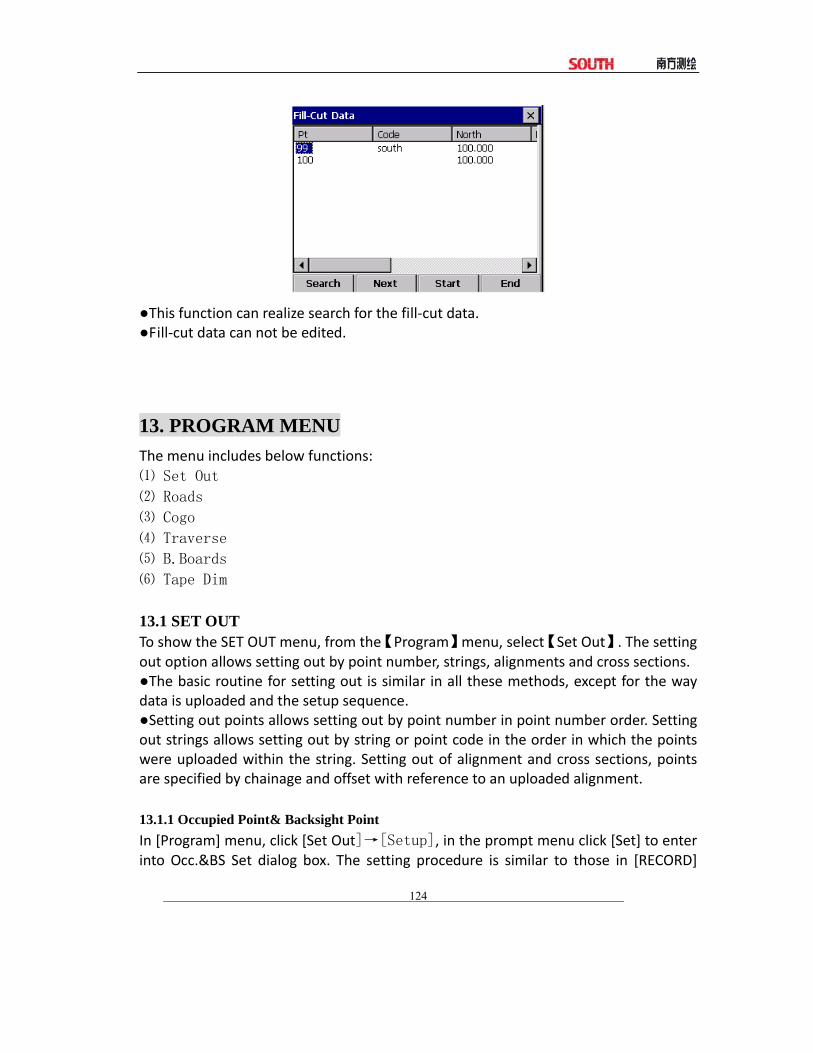
124
●This function can realize search for the fill‐cut data. ●Fill‐cut data can not be edited.
13. PROGRAM MENU The menu includes below functions: ⑴ Set Out
⑵ Roads
⑶ Cogo
⑷ Traverse
⑸ B.Boards
⑹ Tape Dim
13.1 SET OUT To show the SET OUT menu, from the【Program】menu, select【Set Out】. The setting out option allows setting out by point number, strings, alignments and cross sections. ●The basic routine for setting out is similar in all these methods, except for the way data is uploaded and the setup sequence. ●Setting out points allows setting out by point number in point number order. Setting out strings allows setting out by string or point code in the order in which the points were uploaded within the string. Setting out of alignment and cross sections, points are specified by chainage and offset with reference to an uploaded alignment. 13.1.1 Occupied Point& Backsight Point In [Program] menu, click [Set Out]→[Setup], in the prompt menu click [Set] to enter into Occ.&BS Set dialog box. The setting procedure is similar to those in [RECORD]

125
menu. ●If alignment data exists, the occupied point screen changes to include chainage and offset:
●Here the method of using alignment to set occupied point and backsight point will be introduced. Example:
OPERATIONAL STEPS KEY DISPLAY
① In [Program] menu, click
[Setout], in the prompt box click
[Setup] to enter into Occ. &BS Set
screen.
[Set Out]
[Setup]
② If alignment data exists in
internal memory, you can click
[Align] to set the occupied point
Here the method of using alignment
to setup occupied point and azimuth
angle is introduced
In “Occ” field click [Align.] to start
using chainage to setup station
function.
[Align.]
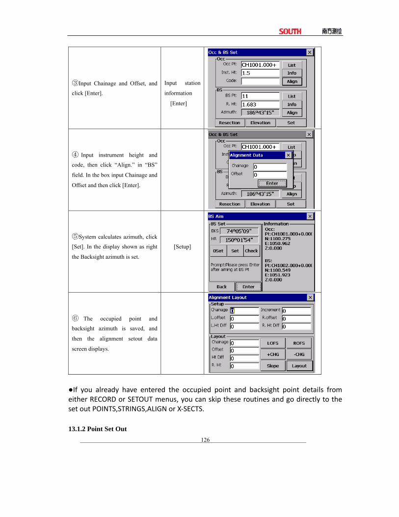
126
③Input Chainage and Offset, and
click [Enter].
Input station
information
[Enter]
④ Input instrument height and
code, then click “Align.” in “BS”
field. In the box input Chainage and
Offset and then click [Enter].
⑤System calculates azimuth, click
[Set]. In the display shown as right
the Backsight azimuth is set.
[Setup]
⑥ The occupied point and
backsight azimuth is saved, and
then the alignment setout data
screen displays.
●If you already have entered the occupied point and backsight point details from either RECORD or SETOUT menus, you can skip these routines and go directly to the set out POINTS,STRINGS,ALIGN or X‐SECTS. 13.1.2 Point Set Out

127
After setting occupied point and backsight point, you can start point setting out Example:
OPERATIONAL STEPS KEY DISPLAY
①In [Program] menu, click [Set
Out], in the prompt box click
[Points].
[Set Out]
[Point]
②In the prompt dialog box input
the PT and Prism Height.
A:
If the coordinates of the point
number exists in memory, system
will call up the point automatically.
B:
If the coordinate data of the point is
not stored in memory, system will
recommends that to input setout
point.
C:
The point to be set out can be
presaved in the project, then click
[List] to call up.
A:
B:
C:

128
③After setting the set out point,
click [Set Out] to start setting out.
Sight the prism center, click
[Measure] to start measure.
※1)
[Set Out]
[Measure]
④ Rotate the telescope, making
“Turn” item and “→” item display
as 0, and ask the rodman to move
the prism.
⑤ Sight the prism center, and
click [Measure] to start measure.
Ask the rod man to move prism
frontward and backward. Making
“Away” item and “↑” item displays
as 0.
[Measure]
⑥ When the four items are
displaying 0, the point to be set out
is found. “Cut” item shows the
value of dig and fill
When it is positive, it means to dig.
When it is minus, it means to fill.

129
⑦After setting out, click [Enter] to
quit The screen displays as the
graph. Repeat steps ②~⑥ to
finish setting out other point.
[Enter]
⑧In PT Layout screen click “ ”
to return to Standard Survey main
menu.
※1) Click [Mode] to choose mode among Fine[s]/Fine [N]/Fine[r]/Track.
Explanation:
Req :The required bearing angle from occupied point to setout point. Turn:The angle that should be rotated. When it is 0, means the bearing angle is correct. Away:The distance from prism to setout point. Positive sign indicates that prism should move far from instrument. Negative sign indicates that prism should move towards instrument. The value means the distance to be moved. Fd : It is the distance along the line of sight to the instrument and is positive away from the instrument. Positive sign means the point is in front of sight line; Positive sign means the point is behind sightline. Right : It is perpendicular to the line of sight with positive to the right when facing the instrument. Positive sign means the point is in the right side of sight line; Positive sign means the point is in the left side of sightline. Cut:The elevation difference of the point. Positive sign indicates that this point is higher than calculated value and it should be cut. Negative sign indicates that it should be filled. The value is the fill‐cut data value. ●Anytime you click “ ” on the upper right screen to return to Pt No screen, you can input a new point and set out next point. Or click [List] to call up data stored in
The ANGLE screen displays the required horizontal angle (Req),
the horizontal angle from the current to the setout point (Turn), the
distance from the prism to the setout point (Away) and the
difference in elevation (Cut).
The OFFSET display shows the distance from the measured point
to the required setout point in the form of offsets.

130
internal memory. If the point is new, system will recommends you to input its coordinate. 13.1.3 String Setout After setting occupied point and backsight point, you can start string setting out Example:
OPERATIONAL STEPS KEY DISPLAY
① In [Program] menu, click [Set
Out], in the prompt menu click
[Strings]
[Set Out]
[Strings]
②Input Chainage and String of the
point to be set out, and click [Set
Out]. System starts to search
automatically. If the string is found,
the first point of this string will be
displayed. As shown in the right
graph, input Target height,Click
[Set Out]. ※1)
[Set Out]
③Sight the prism center and click
[Measure] to start measure. The
setting out method is same as point
setting out.
[Measure]
④After setting out click [Enter] to
quit. The system displays the
second point of the string. Click
[Set Out] to start setting out.
[Enter]
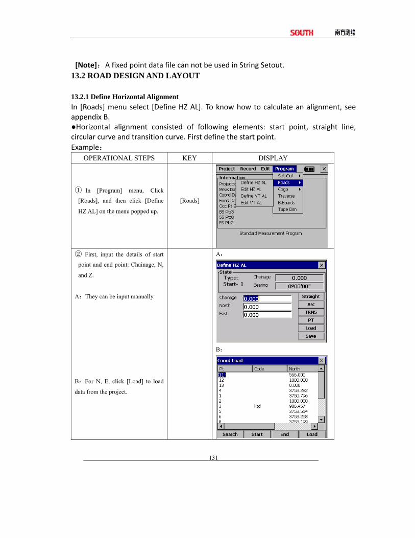
131
[Note]:A fixed point data file can not be used in String Setout. 13.2 ROAD DESIGN AND LAYOUT 13.2.1 Define Horizontal Alignment In [Roads] menu select [Define HZ AL]. To know how to calculate an alignment, see appendix B. ●Horizontal alignment consisted of following elements: start point, straight line, circular curve and transition curve. First define the start point. Example:
OPERATIONAL STEPS KEY DISPLAY
① In [Program] menu, Click
[Roads], and then click [Define
HZ AL] on the menu popped up.
[Roads]
② First, input the details of start
point and end point: Chainage, N,
and Z.
A:They can be input manually.
B:For N, E, click [Load] to load
data from the project.
A:
B:

132
③ After inputting information of
start point, click [Save] to save.
Then enter into the screen of
alignment input process. As shown
on the right.
[Save]
The “Define HZ AL” displays current chainage and the bearing angle (the tangent line from the chainage) and the function key (For creating new line). System provides four functions: defining straight line, circular curve, transition curve, point. Select a function key, enter the detailed information of the chainage, the alignment elements will be created. Click [Save], the new chainage and bearing angle will be calculated automatically and the main alignment screen will be restored. Now other line style can be defined. Press ESC to exit current screen. To modify the element which entered in advance, you should enter the “Edit Alignment” option, the new elements can be added only in the end of the original alignment file. Straight line When the start point or other line style is well‐defined, it allows you to define straight line. A straight line consists of bearing angle and distance; the distance value can not be minus. Example:
OPERATIONAL STEPS KEY DISPLAY
① On the screen of input process,
click [Straight], the screen will
display factors of straight line to be
defined.
[Straight]

133
② Input the bearing and length of
the straight line.
Input bearing
and distance.
③ After inputting, click [Save] to
save the alignment data, and display
the chainage of the end of the line
and its bearing.
· Then, you can define other arcs.
· When the straight line is in the
midst of the alignment, the bearing
of the straight line is calculated on
the base of previous factors. To
modify this bearing, you can input a
new bearing manually.
[Save]
Circular Curve
Click [ARC] in the “Define HZ AL”, the circular curve can be defined. Circular curve consists of Arc length and Radius. The rule of radius value: along the forward direction of the curve. When the curve rotates to right, the radius value is positive. When the curve rotates to left, the radius value is minus. The arc length can not be minus. Example:

134
OPERATIONAL STEPS KEY DISPLAY
① On the screen of input process,
click [ARC]. The screen will
display the factors of arc to be
defined.
[ARC]
② Input radius and arc length.
Input radius
and arc length.
③ After inputting, click [Save] to
save the data of this alignment.
[Save]
Transition curve
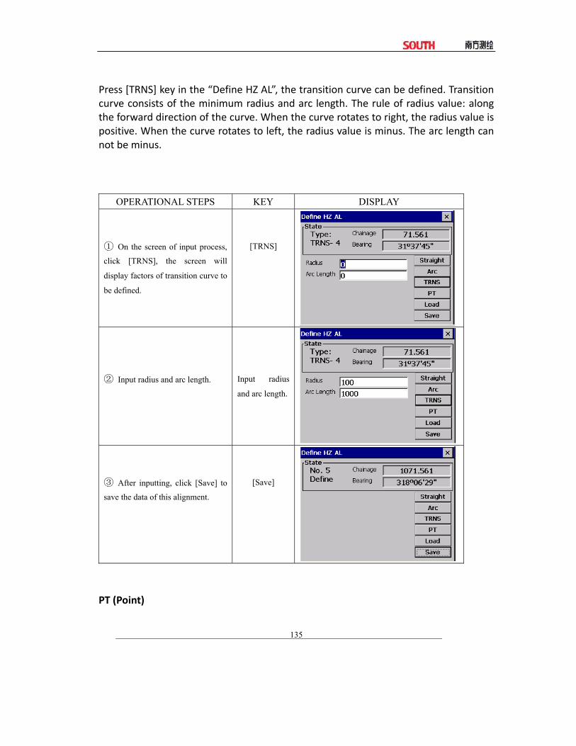
135
Press [TRNS] key in the “Define HZ AL”, the transition curve can be defined. Transition curve consists of the minimum radius and arc length. The rule of radius value: along the forward direction of the curve. When the curve rotates to right, the radius value is positive. When the curve rotates to left, the radius value is minus. The arc length can not be minus.
OPERATIONAL STEPS KEY DISPLAY
① On the screen of input process,
click [TRNS], the screen will
display factors of transition curve to
be defined.
[TRNS]
② Input radius and arc length.
Input radius
and arc length.
③ After inputting, click [Save] to
save the data of this alignment.
[Save]
PT (Point)

136
In “Define HZ AL” menu Click [PT], the point can be defined. A point element consists of coordinates, radius and clothoid parameter A1 and A2. Radius, A1 and A2 can not be minus. If radius is entered, an arc is inserted with the specified radius. If clothoid parameter A1 or A2 is entered, a clothoid is inserted between straight and arc with the specified length. Example:
OPERATIONAL STEPS KEY DISPLAY
① On the screen of input process,
click [PT], the screen will display
factors of point to be defined.
[PT]
② Input N, E, radius and A1, A2.
You can also click [Load] to load
coordinate data from the project.
Input
coordinate,
radius, and arc
factors.

137
③ After inputting, click [Save] to
save the data of this alignment.
[Save]
[NOTE]:When you want to enter A1, A2 from clothoid length L1, L2, the following equations are used:
Any changes to the alignment must be done using the edit alignment option. 13.2.2 Edit Alignment To edit the alignment select Edit HZ AL from the Roads menu.
OPERATIONAL STEPS KEY DISPLAY
① In the menu of [Roads], click
[Edit HZ AL] to enter into the
screen of Edit HZ AL.
[Edit HZ AL]

138
② The screen display the last
alignment data. Search for the data
to be edited.※1)
A:Click Prev. /Next to find the
alignment data to be edited.
B : Click [Search], a dialog as
shown on the right pops up. Input
the chainage and click [Search].
A:
B:
③ System finds the specified
chainage, and displays it on the
screen. Input new data.
④Click any key on the screen,
(such as [Next]), the data is saved.

139
※1) Start:Press this key to go to the start of the file.
End:Press this key to go to the end of the file.
Prev. :Press this key to display the previous point data.
Next :Press this key to display the previous point data.
Search:Press this key to search for data, after pressing this key, enter the required chainage and
press [ENTER], the data for the chainage will be displayed.
[ESC]:Quit the screen.
It is possible to edit data and modify raw data by using above function keys. After entering the data to
be modified, click any operation key on the screen key to record the modified data. To exit without
saving data, press [ESC] key.
13.2.3 Define Vertical Alignment A vertical curve consists of series of intersection points. The intersection point consists of a chainage, elevation and curve length. The start and end intersection points must be a zero curve length.
Chainage 1000 1300 1800 2300 Elevation 50 70 60 90 Curve length 0 300 300 0 Intersection points can be entered in any order. After entering a point data, click [Save] to save the point data and enter next one. Press [ESC] to exit without saving. Example:

140
OPERATIONAL STEPS KEY DISPLAY
①In [Roads] menu click[Define
VT AL] to enter into defining
vertical alignment function.
[Define VT
AL]
② Input chainage, elevation and
Curve Length. After inputting,
click [Save].
The curve length of start and end
point must be 0.
Input
chainage,
elevation and
Curve Length
[Save]
③ The next defining vertical
alignment screen displays.
Continue to input next data.
13.2.4 Edit Vertical Alignment To modify vertical alignment data, the operational steps are same as editing horizontal alignment data.

141
OPERATIONAL STEPS KEY DISPLAY
①In [Roads] menu click [Edit VT
AL] to enter into defining vertical
alignment screen.
[Edit VT AL]
② The screen displays the first
alignment data, search the data
needs to be edited. ※1)
A:Click Prev. /Next to find the
alignment data needed to be edited.
B:Click [Search],a dialog box
pops up as right graph B. Input
chainage and click [Search].
A:
B:
③The specified chainage is found
and displayed on the screen. Input
new data.

142
④Click any key on the screen.
(Such as [Prev.]), the data is
saved.
13.2.5 Alignment Setout
After setting road data, you can start setting out For an alignment setout a horizontal alignment must have been uploaded from
computer by using [Set Out]→[Alignment]. ● the vertical alignment is optional, but is required to compute cut and fill. The
defining method is same as defining horizontal alignment. Rule: Offset left: the horizontal distance from the left stake point to the center line. Offset right: the horizontal distance from the right stake point to the center line. Elevation difference: Left (right) is the elevation difference between left (right)
stake and the center line point.
Example:
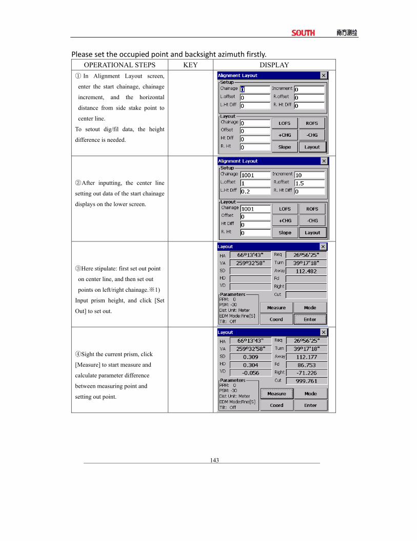
143
Please set the occupied point and backsight azimuth firstly. OPERATIONAL STEPS KEY DISPLAY
① In Alignment Layout screen,
enter the start chainage, chainage
increment, and the horizontal
distance from side stake point to
center line.
To setout dig/fil data, the height
difference is needed.
②After inputting, the center line
setting out data of the start chainage
displays on the lower screen.
③Here stipulate: first set out point
on center line, and then set out
points on left/right chainage.※1)
Input prism height, and click [Set
Out] to set out.
④Sight the current prism, click
[Measure] to start measure and
calculate parameter difference
between measuring point and
setting out point.

144
⑤ Rotate the telescope, making
“Turn” item and “→” item display
as 0, and ask the rodman to move
prism.
⑥ Sight the prism center, click
[Measure] to start measure. Ask the
rodman to move prism making
“Away” and “↑” display as 0.
⑦When four items are 0, the point
to be set out is found. “Cut” item
indicates the dig/fil value.
When it is positive, it means to dig.
When it is minus, it means to fill.
⑧After finish setting out one point,
click [Enter] to quit. The screen
returns to Alignment Setout main
screen.
Click [LOFS]/[ROFS] , or
+CHG/-CHG, repeat steps ②~⑥
to finish setting out other points. ※
1)
※1) Press [LOFS] (or [ROFS]), corresponding chainage, offset, elevation difference will be displayed
on the screen. The chainage and offset can be entered manually. If the offset is minus, the offset point
is at the left side to center line.If the offset is positive, the offset point is at the right side to center line.
Explanation for the main setout screen:
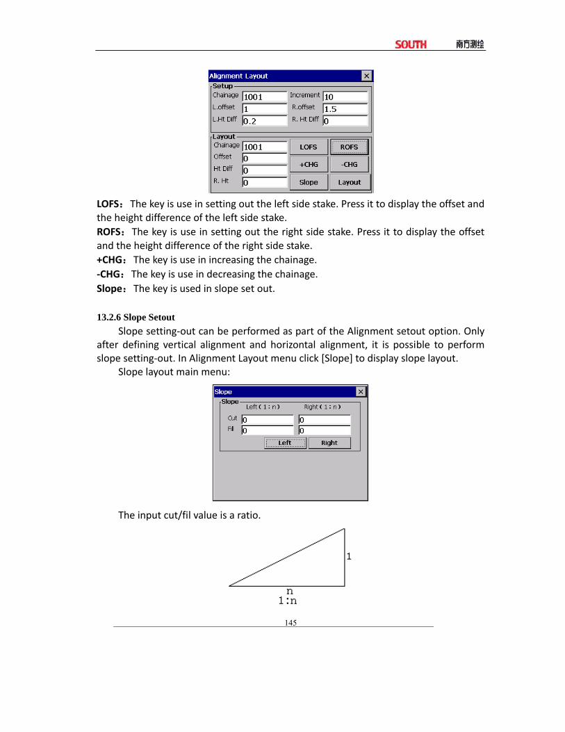
145
LOFS:The key is use in setting out the left side stake. Press it to display the offset and the height difference of the left side stake. ROFS:The key is use in setting out the right side stake. Press it to display the offset and the height difference of the right side stake. +CHG:The key is use in increasing the chainage. ‐CHG:The key is use in decreasing the chainage. Slope:The key is used in slope set out. 13.2.6 Slope Setout
Slope setting‐out can be performed as part of the Alignment setout option. Only after defining vertical alignment and horizontal alignment, it is possible to perform slope setting‐out. In Alignment Layout menu click [Slope] to display slope layout.
Slope layout main menu:
The input cut/fil value is a ratio.
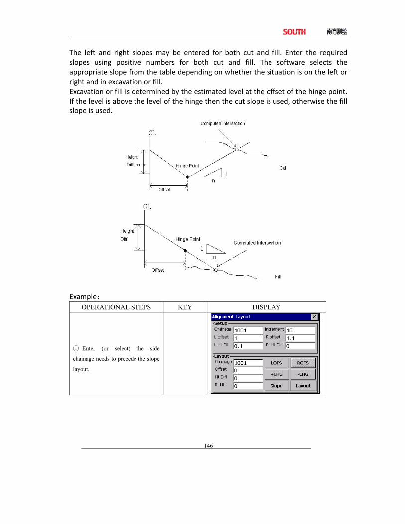
146
The left and right slopes may be entered for both cut and fill. Enter the required slopes using positive numbers for both cut and fill. The software selects the appropriate slope from the table depending on whether the situation is on the left or right and in excavation or fill. Excavation or fill is determined by the estimated level at the offset of the hinge point. If the level is above the level of the hinge then the cut slope is used, otherwise the fill slope is used.
Example: OPERATIONAL STEPS KEY DISPLAY
① Enter (or select) the side
chainage needs to precede the slope
layout.

147
② Click [Slope] to start slope
layout.
After inputting ratio of dig (or fill)
of Left and Right slope After
inputting, select left or right slope
to layout.
[Slope]
③Enter into slope layout menu.
Input the prism pole and sight a
point near where it is estimated the
slope will intercept and press
[Measure] to take the first trial shot.
The appropriate slope is selected
from the data entered in the
preceding step. The appropriate
slope is selected from the data
entered in the preceding step. The
first intercept is computed assuming
a horizontal surface at the level of
the measured point. The error from
measured point to calculated point
will be displayed. The layout
method of slope is same with point
setting out. When the data which
display in [→] and [↑] is 0, the
setting out point is found.
④After laying out the point, click
[Return] to return to slope layout
main menu. Input or select other
slope to layout and layout as the
same method.
[Note]:1) An intersection can not be computed if the ground surface passes through the hinge point.
2) The cut is not displayed because the cut at the computed point is zero.

148
13.2.7 Cross Section Setout To set out design cross sections select X‐Sect from the Set Out menu. The cross section setout is similar to the alignment setout, the points are uploaded in chainage, offset and level format and a reference alignment must also exist.
X‐Sects layout main menu
The screen displays cross section data imported to total station. About the method please refer to “10.2 DATA IMPORT”. Example:

149
OPERATIONAL STEPS KEY DISPLAY
① In the menu of Set Out, click
[X-Sect].
② Data will be displayed on the
screen as shown on the right.
③ Click FNC Key
[+CHG]/[-CHG] to search data
forward or backward; click
[LOFS]/[ROFS] to display
neighboring offset and elevation on
the cross section.
④ Select the chainage to be set
out, and input the prism height of
the target. Then click [Set Out] to
start setting out. The method of
setting out is the same as that of
alignment.
※The Ht.Diff value is elevation value here. (Different to Horizontal Alignment Setting out) [Note]: 1) Cross Section data can not be entered nor edited by manual input; it has to be copied into WIN total station.

150
OPERATIONAL STEPS: ① Create a new text file (.txt) on the computer and save it. See Appendix A for the format of cross section data. ② Copy the file to total station. ③ In the total station, import the saved data to current project by “Data Import”. See “10.2 Data Import”. 2) You can use [LOFS]/[ROFS] to display appointed chainage. The sequence of the displayed data is according to the sequence in text file. Enter the data in the order of its offset values (from left to right), if chainages are the same. 3) When editing the cross section data, chainages should be in the order from little to much. 13.3 COGO The COGO menu contains a number of coordinate geometry functions. (Fixed data can not be used in these functions.) (1.) Intersection (2.) 4‐points intersections (3.) Inverse (4.) Area (5.) Radiation (6.) Missing line Measurement 13.3.1 Intersection The coordinate for a point can be computed by the intersection of two known bearings.
OPERATIONAL STEPS KEY DISPLAY
① In [Program] menu, click
[Cogo]. And click [Intersection] in
Cogo menu.
[Cogo]
[Intersection]

151
② In pop-up dialog input the point
ID and azimuth/distance of point
A, B that are applied in
intersection. Here take azimuth
intersection for example.,※1)、※
2)
If the point ID input does not exist
in the project, an inputting dialog
will display as shown on the right.
Input the coordinate, and click
[Enter] to save.
③ After inputting, click [Calc.],
the system calculate the coordinate
of the intersection.
If there’s no intersection, it displays
“No intersection error”.
Input the point ID, and click
[Enter].
[Calc.]
④ Data is saved. The display
returns to standard survey main
menu.
※1) PT:The number of intersection point.
Azimuth:The azimuth from occupied point to intersection point direction.
Distance:The distance from occupied point to intersection point.
※2) To call up coordinate data from project, you can click [Load].
[NOTE]: If intersection is not in the specified bearing, the software creates the intersection point backward. The intersection point can not be saved, if the coordinates are not in the allowed range 13.3.2 4-Intersection

152
The coordinate for a point can be computed by the intersection of four known points.
OPERATIONAL STEPS KEY DISPLAY
① In COGO menu click
[4-Intersection].
[4-Intersection]
②In the popped up dialog box enter
the points used for 4-Intersection.
If the entered PT doesn’t exist in
project, program will request you to
enter coordinates.
※1)

153
③After inputting, click [Calc.], to
calculate the coordinates of
intersection point.
If no intersection exists, “No
Intersection!” will display.
Input the point name and click
[Enter]
[Calc.]
④The data is saved and the display
returns to standard survey main
menu.
※1) To call coordinate data from project, Click [Load].
[NOTE]: 1) If there is no intersection point, the message “No Intersection” will be displayed. 2) If intersection is not in the specified bearing, the software creates the intersection point backward. 3) The intersection point can not be saved, if the coordinates are not in the allowed range. 13.3.3 Inverse Example:
OPERATIONAL STEPS KEY DISPLAY
①In COGO menu click [Inverse].
[Inverse]
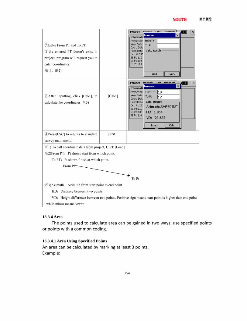
154
②Enter From PT and To PT.
If the entered PT doesn’t exist in
project, program will request you to
enter coordinates.
※1)、※2)
③After inputting, click [Calc.], to
calculate the coordinates ※3)
[Calc.]
④Press[ESC] to returns to standard
survey main menu.
[ESC]
※1) To call coordinate data from project, Click [Load].
※2)From PT:Pt shows start from which point.
To PT:Pt shows finish at which point.
From Pt
To Pt
※3)Azimuth:Azimuth from start point to end point.
HD:Distance between two points.
VD:Height difference between two points. Positive sign means start point is higher than end point
while minus means lower.
13.3.4 Area
The points used to calculate area can be gained in two ways: use specified points or points with a common coding.
13.3.4.1 Area Using Specified Points An area can be calculated by marking at least 3 points. Example:

155
OPERATIONAL STEPS KEY DISPLAY
①In COGO menu click [Area].
[Area]
②A dialog box pops up. Click
“Marked Pt to Calculat” and click
[Enter]. ※1)
[Enter]
③
A:Click [Mark] to mark pts used
for area calc. ※2)
B:You can click [Search] to search
PT in project.
A:
B:
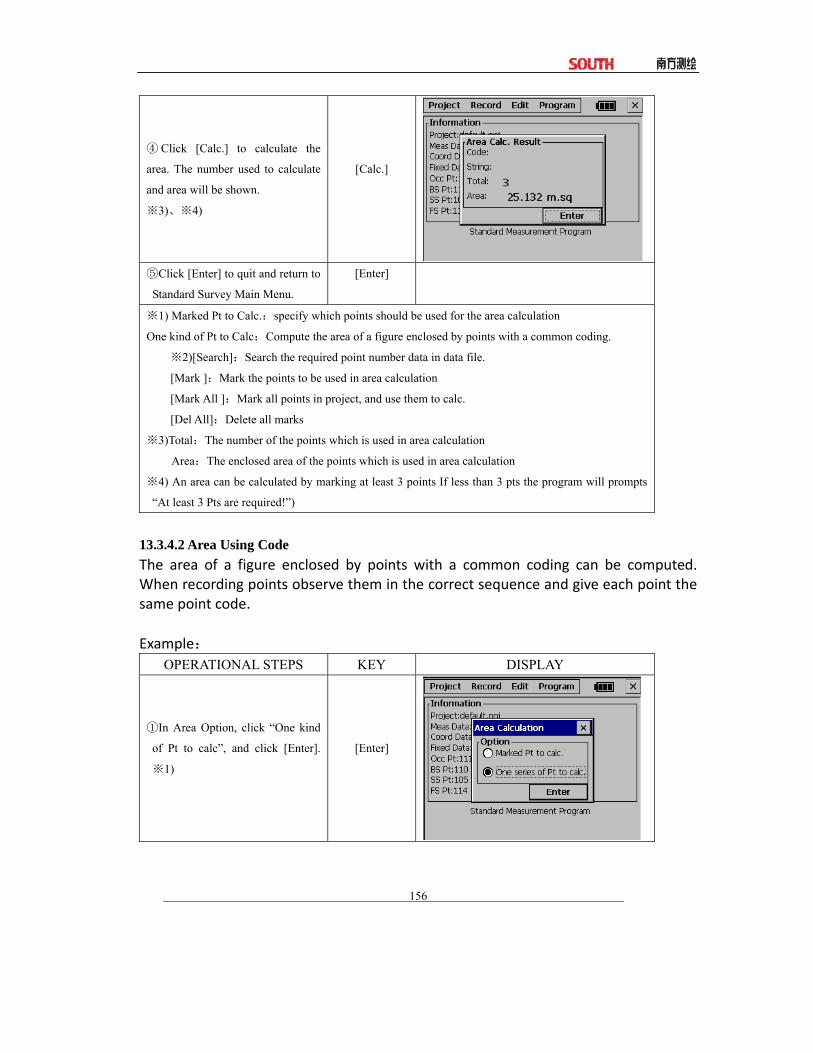
156
④ Click [Calc.] to calculate the
area. The number used to calculate
and area will be shown.
※3)、※4)
[Calc.]
⑤Click [Enter] to quit and return to
Standard Survey Main Menu.
[Enter]
※1) Marked Pt to Calc.:specify which points should be used for the area calculation
One kind of Pt to Calc:Compute the area of a figure enclosed by points with a common coding.
※2)[Search]:Search the required point number data in data file.
[Mark ]:Mark the points to be used in area calculation
[Mark All ]:Mark all points in project, and use them to calc.
[Del All]:Delete all marks
※3)Total:The number of the points which is used in area calculation
Area:The enclosed area of the points which is used in area calculation
※4) An area can be calculated by marking at least 3 points If less than 3 pts the program will prompts
“At least 3 Pts are required!”)
13.3.4.2 Area Using Code The area of a figure enclosed by points with a common coding can be computed. When recording points observe them in the correct sequence and give each point the same point code. Example:
OPERATIONAL STEPS KEY DISPLAY
①In Area Option, click “One kind
of Pt to calc”, and click [Enter].
※1)
[Enter]

157
②Input Code and String used for
area. Click [Enter].
③The program will search data
meets the requirement and
calculate the area.
④Click [Enter] to quit and return to
Standard Survey Main Menu.
[Enter]
Usually (m2 ) or ( ft 2 ) is used as a unit for an area. If the area is larger than
10000m.sq then the unit is changed to Ha (hectare). The unit is changed to AC (acre) if the closed area is 43560ft.sq or more.
[NOTE]:
(1.) Area is not calculated correctly if enclosed lines cross each other. (2.) If less than 3 points are found which have been marked the software will show the
message “3 PTS required”. (3.) The data in fixed points file can not be used in this program. 13.3.5 Missing Line Measurement
This function can be used to calculate the length of a line by measuring the start and end point of this line.
You should set the occupied points and backsight azimuth before the measurement.
Example:

158
OPERATIONAL STEPS KEY DISPLAY
①In Area Option, click [MLM]
[MLM]
② Input the Pt used for MLM
measurement.※1)
(If occupied point and Backsight
azimuth has not been defined, the
dialog box as right will pops up.)
If the entered point doesn’t exist in
project, program will request you to
measure this point.
Set Occ.& BS point:
Pt does not exist in project:

159
③The result is calculated out and
displayed.
dHd:Horizontal distance between
the two points.
dVd:Height difference between
two Points;
dSd:Slope distance between two
points.
④Press [ESC] to quit and return to
Standard Survey Main Menu.
[ESC]
※1) To call coordinate data from project, Click [Load].
[Note]: dVd is defined as the height of the second point minus the height of the first point. Due to this reason dVd can be negative. dSd is defined as the length of the missing line. dHd is defined as the length of the projected missing line in the horizontal plane. dSd and dHd are always positive.
13.3.6 Radiate The coordinate for a point can be computed by entering the Azimuth and Distance.
Example:
OPERATIONAL STEPS KEY DISPLAY
①In COGO menu click [Radiate].
[Radiate]
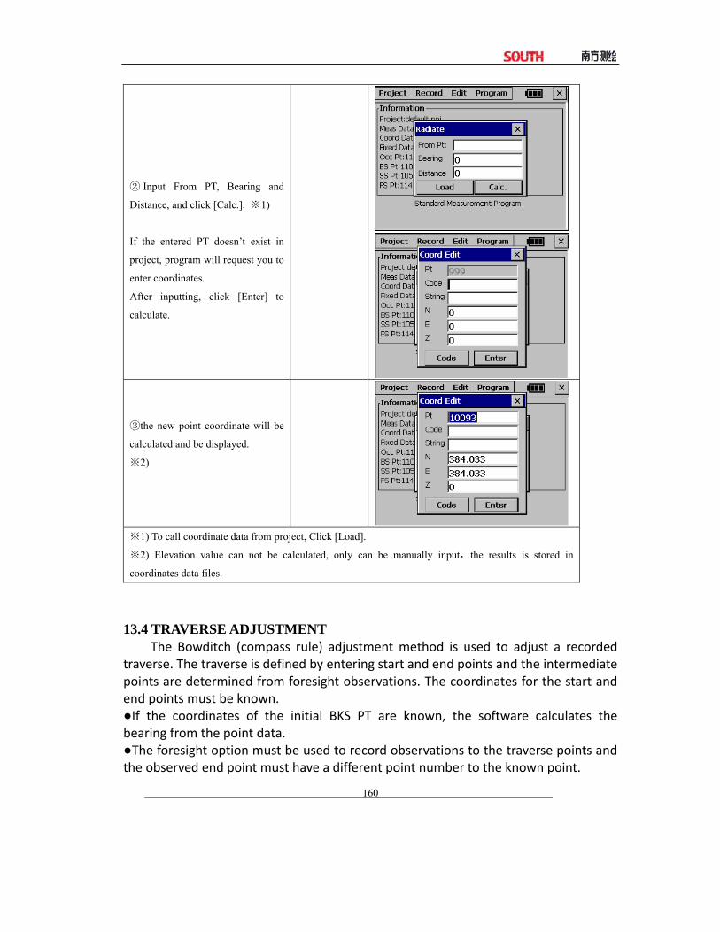
160
② Input From PT, Bearing and
Distance, and click [Calc.]. ※1)
If the entered PT doesn’t exist in
project, program will request you to
enter coordinates.
After inputting, click [Enter] to
calculate.
③the new point coordinate will be
calculated and be displayed.
※2)
※1) To call coordinate data from project, Click [Load].
※2) Elevation value can not be calculated, only can be manually input,the results is stored in
coordinates data files.
13.4 TRAVERSE ADJUSTMENT
The Bowditch (compass rule) adjustment method is used to adjust a recorded traverse. The traverse is defined by entering start and end points and the intermediate points are determined from foresight observations. The coordinates for the start and end points must be known. ●If the coordinates of the initial BKS PT are known, the software calculates the bearing from the point data. ●The foresight option must be used to record observations to the traverse points and the observed end point must have a different point number to the known point.

161
●To adjust angles the end point must be occupied and a known point observed to measure the closing angle. The point number used for this observation must be different from the known point too.
Start Pt: 111 BKS Pt: 110 End Pt: 116 Close Pt: 117 Known Pt: 110 111 916 917
Example: 1. Measurement
OPERATIONAL STEPS KEY DISPLAY
①Select a known point and set up
the instrument on the point. (For
example Pt 111) Set pt 110 as back
sight point. After setting, click
[Set].
② Program calculates out the
Backsight azimuth, click [Setup] to
set current horizontal as the
Backsight azimuth, and click
[Enter].

162
③In [Record] menu click [FS Obs].
[Record]
[FS Obs]
④Sight the traverse point 112, use
[Record] to record the measured
coordinates.
⑤Move the instrument to PT112.
Turn on the machine and select
[Record], remeasure occupied point
(PT112), backsight point (PT111),
sight traverse point (PT113).Click
record.

163
⑥Repeat ①~④ to measure and
record coordinates of each traverse
point. (The number of traverse
point is entered according to length
and requested accuracy).
⑦When the instrument is moved to
PT115, measure a known point
(916), record as PT116.
⑧To calculate traverse, you should
set station on PT116, and sight
another known point (such as
917), measure and record as
PT117. Here the PT117 is the
closing point.
2. Adjustment:
OPERATIONAL STEPS KEY DISPLAY
① In [Program] menu, Click
[Traverse].
[Traverse]

164
② Enter Start Point, and click
[Enter].
Enter start
Point
[Enter]
③When the entered start Point is
same as the start Point in internal
memory, the screen will display a
dialog box to enter end point.
Enter the End Point, (Measured
Point) and known Point, these two
Point must be different.
④ After entering End PT and
known point, click [Enter],
program calculates close
difference. and displays the result.
Click [Enter] to confirm.
⑤Here the screen pops up “Coord
Adjust?” Click [OK] to adjust the
coordinates. Not to change and
data, please click .

165
⑥The screen pops up” Elevation
Adjust?” Here, click [OK] to
adjust. Not to change and data,
please click .
⑦The display returns to standard
survey main menu.
If the closure point is measured: (The step 1, 2 are same as above).
OPERATIONAL STEPS KEY DISPLAY
③After entering Start Pt, system
prompts to enter End Pt (Measured
Point number) and the known Pt,
these two points should be different.
④Enter Close Pt (Measured Point
number) and the known Pt, these
two points should be different too.

166
⑤The close difference is calculated
and displayed.Click [Enter].
⑥The azimuth results display. If
the angle is in the allowed range of
close difference, click [Enter].
⑦ Click [Enter], the system
calculates angle adjustment and
displays the result. Click [Enter].
⑧Here the screen pops up “Coord
Adjust” Press [OK] to adjust Not to
change any data, click“ ”.

167
⑨The screen pops up “Elevation
Adjust” again. Click [OK] to adjust.
Not to change any data, click“ ”.
⑩The display returns to standard
survey main menu.
13.5 BATTER BOARDS
When setting out points, particularly for building plots, it is usually necessary to mark a point with an offset so that the point can be re‐established after work has been carried out in the work area. In this case batter board can be used: the intersection point (of a batter board and the line that connects two points that have to be set out) can be marked. Later, the intersection points are used by pulling a string line between these points. In this way, the required points can be reconstructed.
●There are two ways to proceed: First way is using two sides of the batterboard. The user is advised to use this
method in case high accuracy is required, control of the measurements is required or one batterboard is used to mark more than one intersection point. Refer to Chapter 13.5.1.
Second way is using one side of the batterboard. The user is advised to use this method in case a quick method is required. Refer to Chapter 13.5.2. 13.5.1 Method 1: Batter board using two sides The two sides of batterboard should be measured now. Put the reflector above one side of the batterboard, enter a number for this point (BB point 2) and press Enter. Operating Procedure: (A) Two setout point (S1 and S2) are selected and one side of the batterboard is
measured (BB1). (B) The other side of the batterboard is measured (BB2)。The intersection point of the
batterboard and the line connecting S1 and S2 is calculated. Next, the distance (D1) from BB1 to intersection point and the distance (D2) from BB2 to intersection point are calculated.
(C)

168
Example:
OPERATIONAL STEPS KEY DISPLAY
① In [Program] menu, click
[B.Boards].
②
A:
Input Setout P1 and click [Enter].
B:
If the Point is unknown, a dialog
box will pops up to request you to
enter the coordinates. After
inputting, click [Enter].
A:
B:

169
③Enter Setout P2 and click [Enter].
④
A
Now define the batter board, enter
Board 1 and click [Enter].
B
If the point is unknown, SS
Measurement dialog box will pop
up. After measuring, the data is
record to the project.
A:
B:
⑤Enter Board 2.

170
⑥A dialog box shows the distances
from intersection to PT1 and PT 2.
※1)
⑦Click “OK”, the intersection is
set out.
※1) Click“ ” to quit batter board program.
※The setout of this intersection point is identical to Point Setout, which is discussed in paragraph 13.1.3, except for two differences. 1) Automatically the intersection point is chosen for setting out. 2) CUT is not shown at the screen. NOTE: 1) If the intersection point is not on the batterboard, the message “Point Not on
Batterboard!” is shown on the screen. 2) In case a batterboard is used twice and its position hasn’t changed, it is not
necessary to re‐measure the sides of the batterboard. Use the same number for the sides of the batterboard.
3) The error message “Invalid value !”is shown if the batterboard and the line connecting the two setout points are parallel.
4) The coordinates of the calculated intersection point are recorded in the coordinate file. The number of this intersection point is, compared to the highest existing number, incremented by one.
13.5.2 Method 2: Batterboards using one side Click [S.O.] in case you want to measure only one side of the batterboards.

171
Procedure Operating procedure : (A) Two setout points (S1 and S2) are selected and one side of the batterboard is
measured (BB 1). An approximate distance D1 is shown. (B) The position of the pole is changed according to the value of D1 and a
measurement is performed. The distance D1 is now precise. The process has to be repeated until D equals zero to find the intersection point.
Example: OPERATIONAL STEPS KEY DISPLAY
①After entering Setout Points and
Board1 click [S.O].
②The screen displays as right.
Dist. indicates the distance from the
pole to the intersection point.
Move the pole along the batter
board and click [Measure]. Dist.
now indicates a precise distance.
The intersection point is found
when Dist. equals zero.
NOTE : 1) After the first side of the Batter board has been measured and [S.O.] has been
selected, it is assumed that the orientation of the batter board is perpendicular to
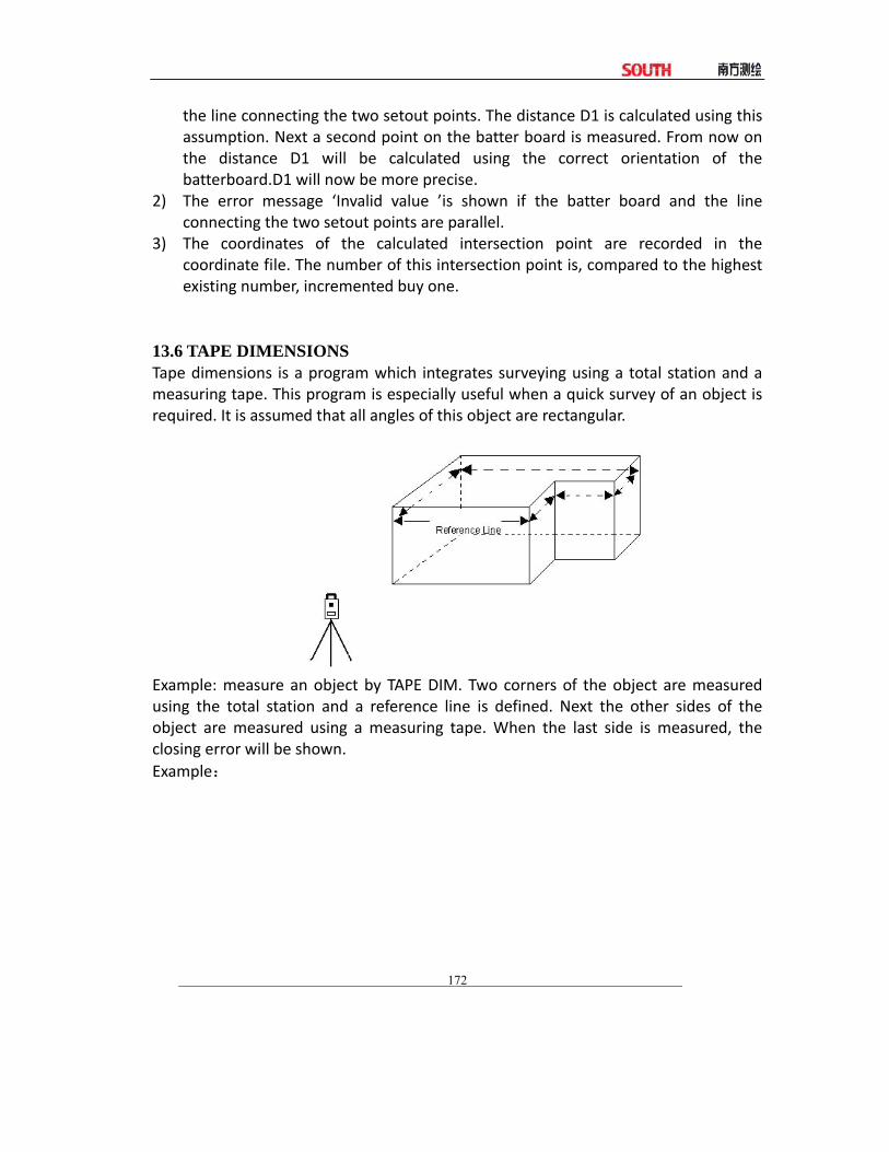
172
the line connecting the two setout points. The distance D1 is calculated using this assumption. Next a second point on the batter board is measured. From now on the distance D1 will be calculated using the correct orientation of the batterboard.D1 will now be more precise.
2) The error message ‘Invalid value ’is shown if the batter board and the line connecting the two setout points are parallel.
3) The coordinates of the calculated intersection point are recorded in the coordinate file. The number of this intersection point is, compared to the highest existing number, incremented buy one.
13.6 TAPE DIMENSIONS Tape dimensions is a program which integrates surveying using a total station and a measuring tape. This program is especially useful when a quick survey of an object is required. It is assumed that all angles of this object are rectangular.
Example: measure an object by TAPE DIM. Two corners of the object are measured using the total station and a reference line is defined. Next the other sides of the object are measured using a measuring tape. When the last side is measured, the closing error will be shown. Example:

173
OPERATIONAL STEPS KEY DISPLAY
①In [Program] menu, Click [Tape
Dim].
②Enter PT A (Start PT) and PT B
(End PT) on Re. line and click
[Enter].
A
If the point exists in project, then
the Re. Line is defined.
A:
B
If the point doesn’t exist in project,
the SS Measurement dialog box
pops up. Measure and record this
point.
B:
③After defining Re. Line, click
[Enter], the screen displays as right.

174
④The reference line is defined,
now use a tape to measure the line
which perpendicular to the
reference line, and start from End
PT of reference line. First select
direction in which the straight line
proceeds and enter Dist, PT and
Code, and click [Enter]. The line is
defined and displayed. If the line is
at the left hand side, press [Left]
key. If the line is at the right hand
side of reference line, press [Right]
key. ※1), ※2)
A:Left
B:Right
⑤ Repeat step ④ and Tape
measure the object in light of its
shape. The new line plus the
reference line are graphically
displayed.
⑥After measuring the last point,
click [End], the screen displays the
misclose.
⑦Click [OK],The display returns
to standard survey main menu.
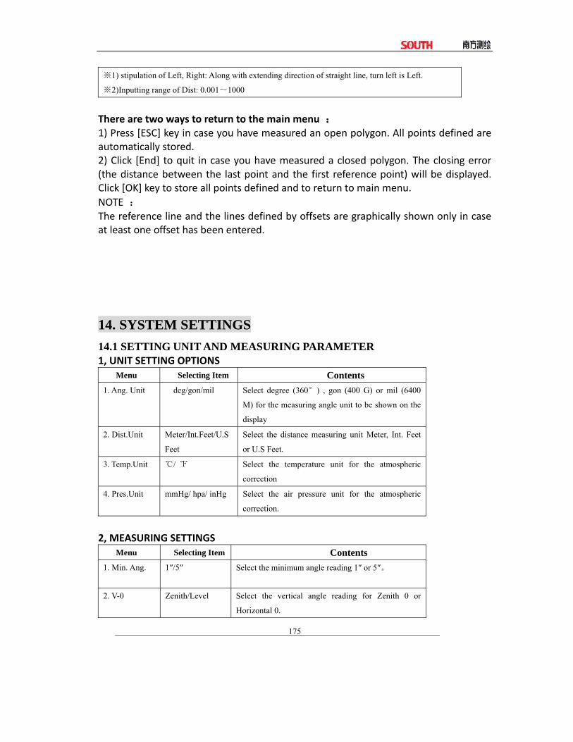
175
※1) stipulation of Left, Right: Along with extending direction of straight line, turn left is Left.
※2)Inputting range of Dist: 0.001~1000
There are two ways to return to the main menu : 1) Press [ESC] key in case you have measured an open polygon. All points defined are automatically stored. 2) Click [End] to quit in case you have measured a closed polygon. The closing error (the distance between the last point and the first reference point) will be displayed. Click [OK] key to store all points defined and to return to main menu. NOTE : The reference line and the lines defined by offsets are graphically shown only in case at least one offset has been entered.
14. SYSTEM SETTINGS 14.1 SETTING UNIT AND MEASURING PARAMETER 1, UNIT SETTING OPTIONS
Menu Selecting Item Contents
1. Ang. Unit deg/gon/mil
Select degree (360°) , gon (400 G) or mil (6400
M) for the measuring angle unit to be shown on the
display
2. Dist.Unit Meter/Int.Feet/U.S
Feet
Select the distance measuring unit Meter, Int. Feet
or U.S Feet.
3. Temp.Unit ℃/ ℉ Select the temperature unit for the atmospheric
correction
4. Pres.Unit mmHg/ hpa/ inHg Select the air pressure unit for the atmospheric
correction.
2, MEASURING SETTINGS
Menu Selecting Item Contents
1. Min. Ang. 1″/5″ Select the minimum angle reading 1″ or 5″。
2. V-0 Zenith/Level Select the vertical angle reading for Zenith 0 or
Horizontal 0.

176
3.Tilt OFF/1axis/2axis Select the tilt sensor option for OFF, (1axis) vertical
only or (2axis) vertical and horizontal
4. W-Corr. 0/0.14/0.20 Select the coefficient correction for refraction and
earth curvature. Selections for the refraction
coefficient are :
OFF( No Correction ) , K =0.14 or K =0.20
※ Correction for atmosphere refraction and the earth curvature
The instrument will automatically correct the effect of atmosphere refraction and the earth curvature when calculating the horizontal distance and the height differences.
The correction for atmosphere refraction and the earth curvature are done by the formulas as follows: Corrected Horizontal Distance:
D=S * [cosα+ sinα* S * cosα (K-2) / 2Re] Corrected Height Differentia:
H= S * [sinα + cosα* S * cosα (1-K) / 2Re]
If the correction of atmosphere refraction and the earth curvature is neglected, the calculation formula of horizontal distance and the height differentia are: D=S∙cosα H=S∙sinα
In formula: K=0.14 ……………………Atmosphere Refraction Modulus
Re=6370 km ………………The Earth Curvature Radius
α (or β) ……………... The Vertical Angle Calculated From Horizontal Plane (Vertical Angle)
S ………………………….Oblique Distance NOTE: The atmosphere refraction modulus of this instrument has been set as: K=0.14. The value of K can be 0.14, 0.2, or shut: (0 VALUE) Example:

177
OPERATIONAL STEPS KEY DISPLAY
①In the main menu click “System
Setup”.
[System Setup]
② Click options of setting
parameter.
③After setting, click [Save].
[Save]
④ Click [OK], the settings are
saved.
[OK]

178
⑤To set Measurement setting, click
“Measurement Setting”, repeat
steps ② ~ ④ to make the
measurement setting. After setting,
click “ ”.
14.2 SETTING ATMOSPHERE DATA AND PRISM CONSTANT Atmospheric Parameters (ppm): The speed of light in air is extremely fast. And it is not a constant, but changes with the temperature and pressure of atmosphere. Once atmosphere correction is set, this instrument can implement atmosphere correction automatically. Even the instrument is powered off, the atmosphere correction value is still kept. ●You can set the atmosphere correction value under star key(★) mode. ●The formula of atmosphere correction: (unit: meter)) PPM = 273.8 ‐ 0.2900 × pressure value(hPa) 1 + 0.00366 × temperature value(℃) If the pressure unit is mmHg: 1hPa = 0.75mmHg ●When disregard atmosphere correction, set PPM value as 0. ●Standard atmospheric condition of Total Station (i.e. the atmospheric condition that the atmosphere correction value of the instrument is 0): Pressure: 1013 hPa Temperature: 20℃ Prism Constant
Since the constants of prisms manufactured by different companies are different, the corresponding prism constant must be set. Once the prism constant is set, it would be kept even if the machine is turned off.
Example:

179
OPERATIONAL STEPS KEY DISPLAY
① In System Setting click
“Atmospheric Parameter”.
②The screen shows the parameter
current used. Enter new data in the
fields you need to set.
③After setting, click [Save].
[Save]
④ Click [OK], the settings are
saved.
[OK]
※1)Data range: Temperature:-30 ~ +60℃ (Feet length 0.1℃) or -22 ~ +140℉(feet length1
℉)
Pressure:420 ~ 800mmHg(Feet length 1mmHg) or 560 ~ 1066 hPa(Feet length 0.1hpa)
16.5 ~ 31.5 inchHg (Feet length 0.1 inchHg)

180
PPM:-100 ~ +100 PPM (Feet length 1PPM)
PSM:-100 ~ +100 mm (Feet length 1mm)
※2) The instrument will calculate PPM according to the entered Temperature and Pressure.
15. CHECK AND ADJUSTMENT This instrument has undergone a strict process of checking and adjustment,
which ensures that it meets quality requirement. However, after long periods of transport or under a changing environment, there may be some influences on the internal structure. Therefore, before the instrument is used for the first time, or before precise surveys, user should launch check and adjustment introduced in this chapter to ensure the precision of the job.
15.1 PLATE VIAL
Check Please refer to Chapter 3.2 “Leveling by Using Plate Vial” Adjust 1. Adjust leveling screws, make plate bubble centered; 2. Rotate the instrument 180°; watch the offset of plate level; 3. Tweak adjustment screws (on the right of the plate vial) with the correction pin to make plate bubble to move half of the offset back; 4. Rotate the instrument 180°, check adjustment result; 5. Repeat the above steps until the plate level is centered in all directions. 15.2 CIRCULAR VIAL Check:
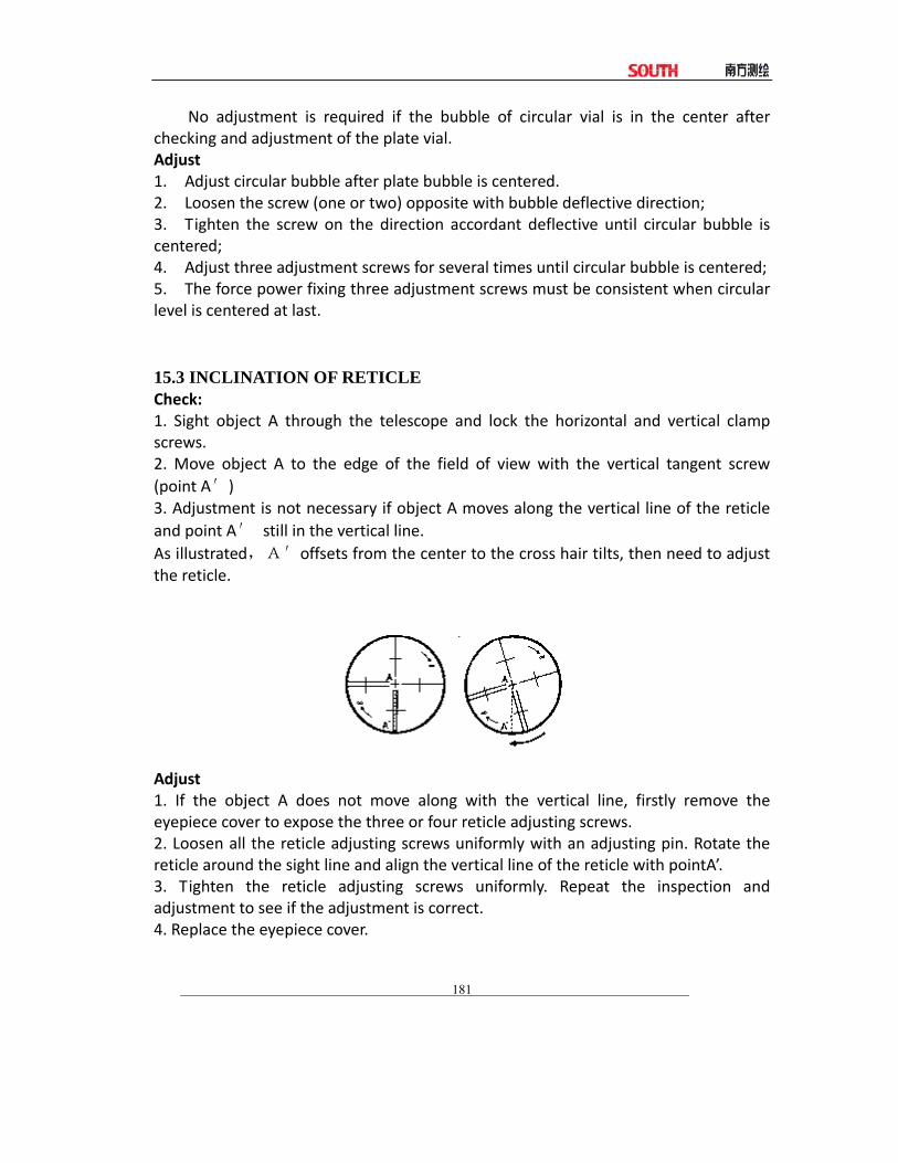
181
No adjustment is required if the bubble of circular vial is in the center after checking and adjustment of the plate vial. Adjust 1. Adjust circular bubble after plate bubble is centered. 2. Loosen the screw (one or two) opposite with bubble deflective direction; 3. Tighten the screw on the direction accordant deflective until circular bubble is centered; 4. Adjust three adjustment screws for several times until circular bubble is centered; 5. The force power fixing three adjustment screws must be consistent when circular level is centered at last. 15.3 INCLINATION OF RETICLE Check: 1. Sight object A through the telescope and lock the horizontal and vertical clamp screws. 2. Move object A to the edge of the field of view with the vertical tangent screw (point A′) 3. Adjustment is not necessary if object A moves along the vertical line of the reticle and point A′ still in the vertical line. As illustrated,A′offsets from the center to the cross hair tilts, then need to adjust the reticle.
Adjust 1. If the object A does not move along with the vertical line, firstly remove the eyepiece cover to expose the three or four reticle adjusting screws. 2. Loosen all the reticle adjusting screws uniformly with an adjusting pin. Rotate the reticle around the sight line and align the vertical line of the reticle with pointA’. 3. Tighten the reticle adjusting screws uniformly. Repeat the inspection and adjustment to see if the adjustment is correct. 4. Replace the eyepiece cover.

182
15.4 PERPENDICULARITY BETWEEN LINE OF SIGHT AND HORIZONTAL AXIS (2C) Check 1. Set object A at about 100 meters away the same height as the instrument, and make the vertical angle with ±3°. Then level and center the instrument and turn on the power 2. Sight object A in FaceI and read the horizontal angle value. (e.g.: Horizontal angle L=10°13′10″). 3. Loosen the vertical and horizontal clamp screws and rotate the telescope. Sight object A in Reverse faceand read the horizontal angle value. (e.g.: Horizontal angle R= 190°13′40″). 4. 2C=L‐R±180°=‐30″≥±20″, adjustment is necessary. Adjust A. Electronic Adjustment Operation Steps:
OPERATIONAL STEPS KEY DISPLAY
①After leveling the instrument, in
the main menu click [System
Setup].

183
② In the menu bar click to
show Collimation as right.
③In Face I precisely collimate the
target, and press [Set].
Collimate the
target
[Set]
④ Rotate the telescope and
precisely sight the same target in
Reverse face. Click [Set].
Sight prism in
Reverse face
+
[Set]
⑤After setting, the screen displays
as right. Click [Set].
[Set]

184
⑥Click [OK] to finish adjustment
of collimation.
[OK]
B. Optics Adjustment (professional maintenance man only) 1. Use the tangent screw to adjust the horizontal angle to the right reading which has been eliminated C, R+C=190°13′40″‐15″=190°13′25″ 2. Take off the cover of the reticle between the eyepiece and focusing screw. Adjust the left and right adjusting screws by loosening one and tightening the other. Move the reticle to sight object A exactly. 3. Repeat inspection and adjustment until|2C|<20". 4. Replace the cover of the reticle. Note: After adjustment, need to check the photoelectricity coaxiality. 15.5 VERTICAL INDEX DIFFERENCE COMPENSATION Check 1. Mount and level the instrument and make the telescope parallel with the line connecting the center of the instrument to any one of the screws. Lock the horizontal clamp screw. 2. After turning on the power, zero the vertical index. Lock the vertical clamp screw and the instrument should display the vertical angle value. 3. Rotate the vertical clamp screw slowly in either direction about 10mm in circumference, and the error message “b” will appear. The vertical axis inclination has exceeded 3ˊat this time and exceeds the designated compensation range. 4. Rotate the above screw to its original position, and the instrument display screen will show the vertical angle again, meaning that the vertical index difference compensation function is working. Adjust
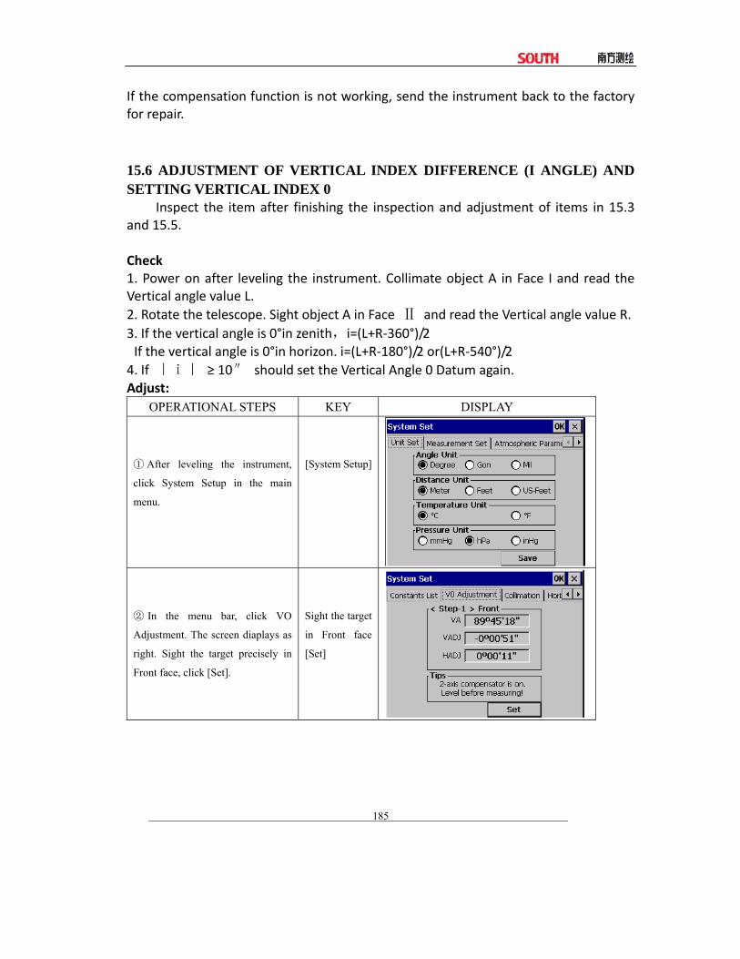
185
If the compensation function is not working, send the instrument back to the factory for repair. 15.6 ADJUSTMENT OF VERTICAL INDEX DIFFERENCE (I ANGLE) AND SETTING VERTICAL INDEX 0
Inspect the item after finishing the inspection and adjustment of items in 15.3 and 15.5. Check 1. Power on after leveling the instrument. Collimate object A in Face I and read the Vertical angle value L. 2. Rotate the telescope. Sight object A in Face Ⅱ and read the Vertical angle value R. 3. If the vertical angle is 0°in zenith,i=(L+R‐360°)/2 If the vertical angle is 0°in horizon. i=(L+R‐180°)/2 or(L+R‐540°)/2 4. If |i| ≥ 10″ should set the Vertical Angle 0 Datum again. Adjust:
OPERATIONAL STEPS KEY DISPLAY
① After leveling the instrument,
click System Setup in the main
menu.
[System Setup]
② In the menu bar, click VO
Adjustment. The screen diaplays as
right. Sight the target precisely in
Front face, click [Set].
Sight the target
in Front face
[Set]

186
③ Rotate the telescope and
precisely sight the same target in
Reverse face. Click [Set].
Sight prism in
Reverse face
[Set]
④After setting, the screen displays
as right. Click [Set].
[Set]
⑤Click [OK] to finish adjustment
of index error.
[OK]
Note: 1. Repeat the checking steps to measure the Index Error (i angle). If the Index Error cannot meet the requirement; user should check whether the three steps of the adjustment and the collimation are right. Then set again according to the requirement. 2. If Index Error still not meets the requirement after the repeated operation, the instrument should be returned to factory for inspection and repair. ● The vertical angle displayed in zero point setting has not been compensated or modified, only for reference during setting. 15.7 TRANSVERSE AXIS ERROR COMPENSATION ADJUSTMENT
As the transverse axis error only affects the angle of sight, it can be only confirmed through observing the target the height of which is obviously lower or

187
higher than the instrument. To avoid the influence of sight axis, user must have an associated adjustment
before adjusting sight axis. It is unnecessary to collimate the prism or the target plane to ascertain the
transverse axis error. Therefore user is enabled to launch this adjustment at any time. Select a recognizable point which is rather far away from the instrument, and much higher or lower than the instrument. Make sure it can be precisely collimated twice.
OPERATIONAL STEPS KEY DISPLAY
① After leveling the instrument,
click System Setup in the main
menu.
[System Setup]
②In the menu bar click Horizontal
Axis. The screen displays as right.
Sight the target precisely in front
face, Click [Set] 10 times.
Sight the prism
in front face,
Click [Set] 10
times
③ Rotate the telescope and
precisely sight the same target in
reverse face . Click [Set] 10 times.
sight the same
target in
reverse face
Click [Set] 10
times
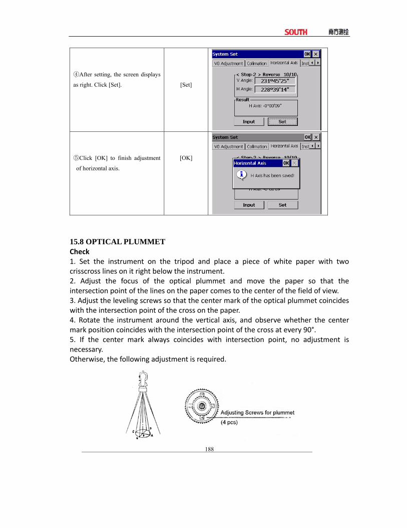
188
④After setting, the screen displays
as right. Click [Set].
[Set]
⑤Click [OK] to finish adjustment
of horizontal axis.
[OK]
15.8 OPTICAL PLUMMET Check 1. Set the instrument on the tripod and place a piece of white paper with two crisscross lines on it right below the instrument. 2. Adjust the focus of the optical plummet and move the paper so that the intersection point of the lines on the paper comes to the center of the field of view. 3. Adjust the leveling screws so that the center mark of the optical plummet coincides with the intersection point of the cross on the paper. 4. Rotate the instrument around the vertical axis, and observe whether the center mark position coincides with the intersection point of the cross at every 90°. 5. If the center mark always coincides with intersection point, no adjustment is necessary. Otherwise, the following adjustment is required.
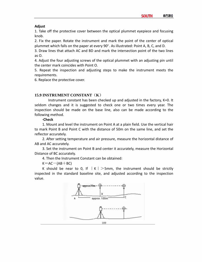
189
Adjust 1. Take off the protective cover between the optical plummet eyepiece and focusing knob. 2. Fix the paper. Rotate the instrument and mark the point of the center of optical plummet which falls on the paper at every 90°. As illustrated: Point A, B, C, and D. 3. Draw lines that attach AC and BD and mark the intersection point of the two lines as O. 4. Adjust the four adjusting screws of the optical plummet with an adjusting pin until the center mark coincides with Point O. 5. Repeat the inspection and adjusting steps to make the instrument meets the requirements. 6. Replace the protective cover. 15.9 INSTRUMENT CONSTANT(K)
Instrument constant has been checked up and adjusted in the factory, K=0. It seldom changes and it is suggested to check one or two times every year. The inspection should be made on the base line, also can be made according to the following method.
∙Check 1. Mount and level the instrument on Point A at a plain field. Use the vertical hair
to mark Point B and Point C with the distance of 50m on the same line, and set the reflector accurately.
2. After setting temperature and air pressure, measure the horizontal distance of AB and AC accurately.
3. Set the instrument on Point B and center it accurately, measure the Horizontal Distance of BC accurately.
4. Then the Instrument Constant can be obtained: K=AC-(AB+BC) K should be near to 0, If |K|>5mm, the instrument should be strictly
inspected in the standard baseline site, and adjusted according to the inspection value.
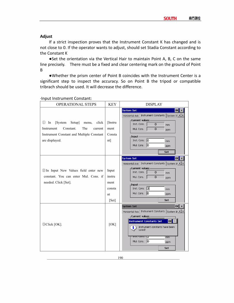
190
Adjust
If a strict inspection proves that the Instrument Constant K has changed and is not close to 0. If the operator wants to adjust, should set Stadia Constant according to the Constant K
●Set the orientation via the Vertical Hair to maintain Point A, B, C on the same line precisely. There must be a fixed and clear centering mark on the ground of Point B
●Whether the prism center of Point B coincides with the Instrument Center is a significant step to inspect the accuracy. So on Point B the tripod or compatible tribrach should be used. It will decrease the difference. ∙Input Instrument Constant:
OPERATIONAL STEPS KEY DISPLAY
① In [System Setup] menu, click
Instrument Constant. The current
Instrument Constant and Multiple Constant
are displayed.
[Instru
ment
Consta
nt]
② In Input New Values field enter new
constant. You can enter Mul. Cons. if
needed. Click [Set].
Input
instru
ment
consta
nt
[Set]
③Click [OK].
[OK]

191
1※ ) Horizontal compensation adjust, vertical compensation and EDM adjusting: are set by the factory,
please do not make any setting.
15.10 PARALLEL BETWEEN LINE OF SIGHT AND EMITTING PHOTOELECTRIC AXIS Check: 1. Set the reflector 50m away from the instrument. 2. Collimate the center of the reflector prism with reticle. 3. Switch on the instrument, and enter into Distance Measurement Mode. Press [DIST] (or [All]) to measure. Rotate the Horizontal Tangent Screw and Vertical Tangent Screw to launch electric collimation and make the light path of EDM unblocked. In the bright zone find the center of emitting photoelectric axis. 4. Check the center of reticle to coincide with the center of emitting photoelectric axis. If so, the instrument is proved eligible.
Adjustment: If the center of reticle deviates from the center of emitting photoelectric axis, user should sent the instrument to
professional repair department. 15.11 TRIBRACH LEVELING SCREW
If the leveling screw appears flexible, adjust the two adjusting screw in the leveling screw to tighten the screw appropriately.
15.12 RELATED PARTS FOR REFLECTOR 1. The Tribrach and Adapter for Reflector The plate vial and optical plummet in the adapter and tribrach should be checked. Refer to Chapter 15.1 and 15.8 for more information. 2. Perpendicularity of the prism pole
As illustrated in Chapter 15.8, mark ‘+’ on Point C, place the tine of the prism pole on the Point C and do not move during the inspection. Place the two feet tine of Bipod on the cross lines of Point E and F. Adjust the two legs “e’ and “f” to make the bubble on the prism pole centered.
Set and level the instrument on Point A near the cross. Sight the tine of Point C

192
with the center of reticle, and fix the Horizontal Clamp Screw. Rotate the telescope upward to make D near the horizontal hair. Flex the prism pole Leg “e” to make the D in the center of reticle. Then both Point C and D are on the central line of reticle.
Set the instrument on Point B to another cross lines. With the same way to flex the Leg “f” to make Point C and D on the central line of reticle.
Through the adjustment of the instrument on Point A and B, prism pole has been perpendicular. If the bubble offsets from the center, adjust the three screws under circular vial to make the bubble centered.
Check and adjust again until the bubble is in the center of the vial from both directions of the prism pole.

193
16. ACCESSORIES
Carrying Case 1pc Main Body 1pc Backup on‐board Battery 1pc Charger 1pc Plummet 1pc Correction Pin 2 pcs Fur Brush 1pc Screwdriver 1pc Allen key 2 pcs Cloth 1pc Dryer 1pc Operation Manual 1pc Certificate 1pc Stylus pen 2 pc USB data line 1 pc

194
【APPENDIX-A】 1 EXPORT DATA FROM TOTAL STATION
After saving the data collected by total station by “Data Export” to appointed route, use U disk or synchronizing software (use Microsoft ActiveSync to synchronize total station and PC.) to copy to your computer, then you can view the data.
1.1 Raw Data Format WinCE (Identifier) (Included information)
PROJECT Project name, description of file saving path. DATE Date & time NAME name of the surveyor INST Serial number of instrument UNITS (unit)meter/feet/US‐feet,degree, gon, mil SCALE Grid factor, scale, and height ATMOS Temp (℃), press (hPa) STN point ID,instrument height,identifier of station PT XYZ X(E),Y(N), Z(H) BKB Point number,Backsight azimuth,Backsight angle BS Point number[,Target height] FS Point number,Target height,Point number coding[,String] SS Point number,Target height,Point numbercoding[,String] CTL control code[,point code 2[,String]](optional) HV HA(Horizontal angle),VA(Vertical angle) SD HA(Horizontal angle),VA(Vertical angle),SD(Slanting distance) HD HA(Horizontal angle),HD(horizontal distance),VD(Height
differentia) NOTE note RES OBS Point number,Target height,observation times
1.2 Coordinate Data Format Point number, E,N,H,code 111,1.059,1.059,1.298,, 112,1.000,1.000,2.596,, 113,1.059,1.059,1.297,, 114,1.059,1.059,1.297,,
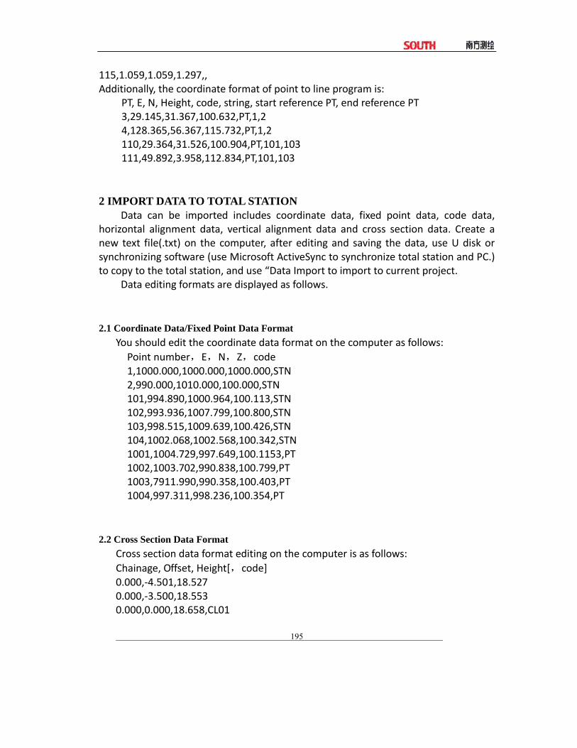
195
115,1.059,1.059,1.297,, Additionally, the coordinate format of point to line program is: PT, E, N, Height, code, string, start reference PT, end reference PT 3,29.145,31.367,100.632,PT,1,2 4,128.365,56.367,115.732,PT,1,2 110,29.364,31.526,100.904,PT,101,103
111,49.892,3.958,112.834,PT,101,103
2 IMPORT DATA TO TOTAL STATION
Data can be imported includes coordinate data, fixed point data, code data, horizontal alignment data, vertical alignment data and cross section data. Create a new text file(.txt) on the computer, after editing and saving the data, use U disk or synchronizing software (use Microsoft ActiveSync to synchronize total station and PC.) to copy to the total station, and use “Data Import to import to current project.
Data editing formats are displayed as follows.
2.1 Coordinate Data/Fixed Point Data Format You should edit the coordinate data format on the computer as follows: Point number,E,N,Z,code 1,1000.000,1000.000,1000.000,STN 2,990.000,1010.000,100.000,STN 101,994.890,1000.964,100.113,STN 102,993.936,1007.799,100.800,STN 103,998.515,1009.639,100.426,STN 104,1002.068,1002.568,100.342,STN 1001,1004.729,997.649,100.1153,PT 1002,1003.702,990.838,100.799,PT 1003,7911.990,990.358,100.403,PT 1004,997.311,998.236,100.354,PT 2.2 Cross Section Data Format Cross section data format editing on the computer is as follows:
Chainage, Offset, Height[,code] 0.000,‐4.501,18.527 0.000,‐3.500,18.553 0.000,0.000,18.658,CL01

196
0.000,3.500,18.553 0.000,5.501,18.493 12.669,‐4.501,18.029 12.669,‐3.500,18.059 12.669,‐0.000,18.164,CL01 12.669,3.500,18.059 12.669,5.501,17.999
2.3 Point P Coding Format The code files enclosed in code library, should assure that every line has a code, which includes entity number and layer name, etc. Every entity is ended by carriage return. The edited coding format is as follows:
Code[,Entity[,Layer]] TREE,1,VEG FENCE,2,BDY CL,2,CL EP,2,ROAD GUTTER,2,ROAD PATH,2,PATH DRAIN,2,DRAIN BM,1,CONTROL MH,1,DRAIN GUS,1,UTILITY WATER,2,UTILITY LP,1,UTILITY LIGHTS,1,UTILITY ROCK,2,NS
●When there is no definition in code library, the default value for entity is “1”, and for layer is “0”.
2.4 Horizontal Line The horizontal line is transmitted from computer to instrument through line element, including initial definition. It should be included in initial definition the number of the start stake and coordinate of this point. The line elements include point, straight, arc, and transition curve. Each recorded format is:
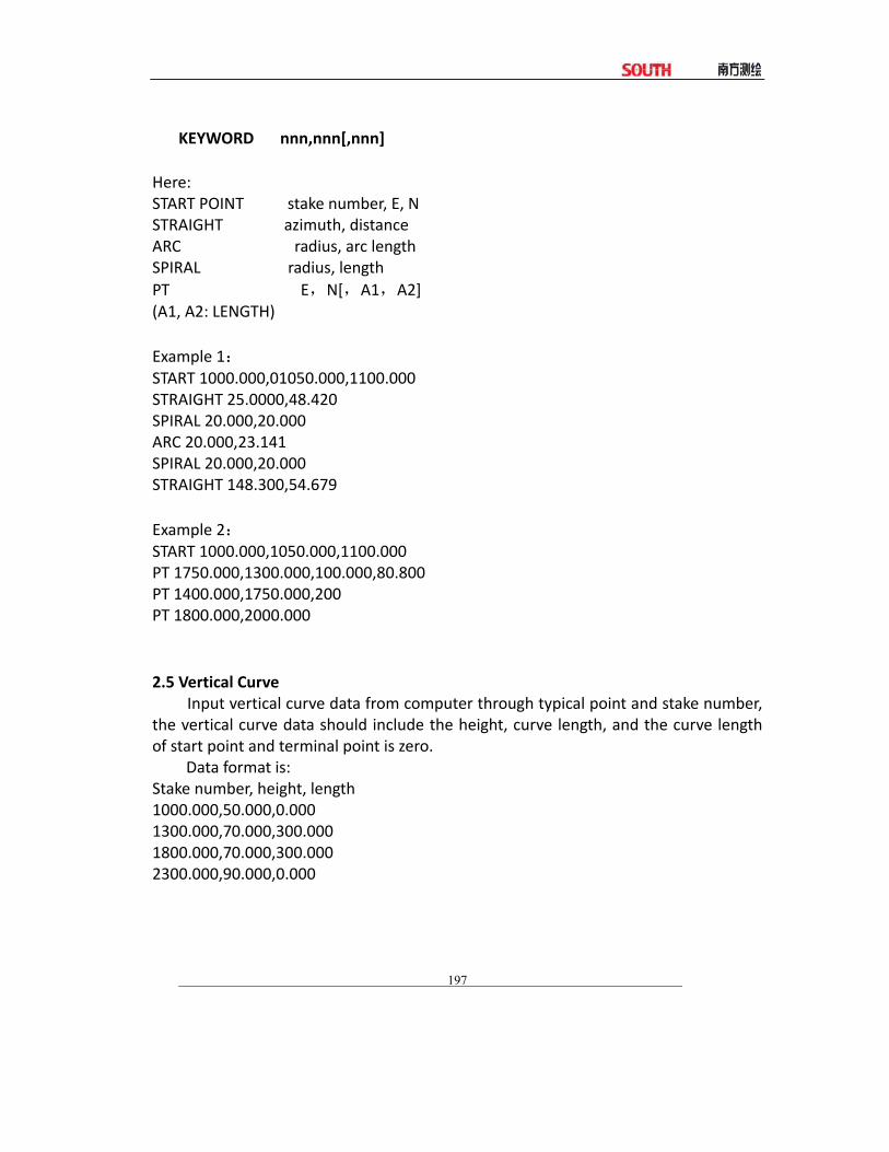
197
KEYWORD nnn,nnn[,nnn] Here: START POINT stake number, E, N STRAIGHT azimuth, distance ARC radius, arc length SPIRAL radius, length PT E,N[,A1,A2] (A1, A2: LENGTH) Example 1: START 1000.000,01050.000,1100.000 STRAIGHT 25.0000,48.420 SPIRAL 20.000,20.000 ARC 20.000,23.141 SPIRAL 20.000,20.000 STRAIGHT 148.300,54.679 Example 2: START 1000.000,1050.000,1100.000 PT 1750.000,1300.000,100.000,80.800 PT 1400.000,1750.000,200 PT 1800.000,2000.000 2.5 Vertical Curve
Input vertical curve data from computer through typical point and stake number, the vertical curve data should include the height, curve length, and the curve length of start point and terminal point is zero.
Data format is: Stake number, height, length 1000.000,50.000,0.000 1300.000,70.000,300.000 1800.000,70.000,300.000 2300.000,90.000,0.000

198
【APPENDIX-B】 CALCULATE ROAD ALIGNMENT The road alignment stake‐out program can stake out the alignment elements including straight, arc and transition curve. NOTE: ●Road alignment data can be uploaded from computer or can be entered manually. Transect data can only be uploaded from computer. ●Road alignment and transect data is managed by chainage. ●One job corresponds to one road alignment, you can use several jobs to create several alignments. 1 ROAD ALIGNMENT ELEMENTS There are two ways to enter the alignment elements: 1) Download from PC. 2) Manually entered on the WinCE (R) series. How to enter the alignment data is explained below:
Alignment Element Parameter
Straight Bearing, Distance
Transition Curve Radius, Length of Transition
Curve
Arc Radius, Length of Arc
PT N, E, radius, A1, A2
NOTE: When downloading from computer or selecting PT option, you do not have to calculate the Parameter.

199
Pt North East Radius Transition curve A1 Transition curve A2 (N) (E) (R) BP 1100.000 1050.000 IP1 1300.000 1750.000 100.000 80.000 80.000 IP2 1750.000 1400.000 200.000 0.000 0.000 EP 2000.000 1800.000 Example: To enter the following data select DEF AL of ROADS in PROG menu: CH 0 N 1100.000 E 1050.000 Press [ENT] and then click (PT) on the screen, Enter the following data: N 1300.000 E 1750.000 R 100.000 A1 80.000 A2 80.000 Enter the following data in the above way: N 1750.000 E 1400.000 R 200.000 A1 0.000 A2 0.000 N 2000.000 E 1800.000
R 0.000 A1 0.000 A2 0.000 The format of the data above transmitted to computer is as follows: START 0.000,1050.000,1100.000 CRLF PT 1750.000,1300.000,100.000,80.000,80.000 CRLF PT 1400.000,1750.000,200.000,0.000,0.000 CRLF PT 1800.000,1800.000,2000.000 CRLF

200
2 CALCULATION ROAD ALIGNMENT ELEMENTS ⑴ Calculation of the length of transition curve
L 2.1 =RA2
2.1 L 2.1 : Length of clothoid
A 2.1 : Parameter of clothoid R : Radius
L1 = RA2
1 =100802
=64 m L2 = RA2
2 =100802
=64 m
⑵ Calculation of Deflection Angle
τ =AL
2
2
2
τ 1= 8064
2
2
2 ⋅= 0.32 rad ⇒ deg ⇒ 0.32
π180 =18°20′06″
∴ τ 1= ‐τ 2 ⑶ Calculation of transition coordinates
τ2⋅= AN ....)936021610
1(642 τττ −+−
τ2⋅= AE ....)75601320423
(753 ττττ
−+−
32.0280 ⋅⋅=N ....)936021610
1( )32.0()32.0()32.0( 642
−+−
)9360
40010734182.0216
01048576.010
01024.01(64 −+−=
)00000011.000004855.001024.01(64 −+−= =64 * 0.98981 =63.348 Similarly, the value of E is:
32.0280 ⋅⋅=E ....)75601320423
32.0()32.0()32.0()32.0( 753
−+−
)00000025.000078019.010666667.0(64 −+−= =6.777 This example is symmetry spiral transition N1=N2,E1=E2 ⑷Calculation of shift value RΔ
)cos1( τ−−=Δ RER

201
18cos1(100777.6 −−=ΔR °20′06″) =1.700 Symmetry spiral transition RR 21 Δ=Δ ⑸ Calculation of Spiral Transition coordinate τsinRNN m −= =63.348‐100sin18°20′06″=31.891 Symmetry spiral transition NN mm 21 = ⑹ Calculation of Tangent Distance
NRRD mLALAecLAR 1121 )cot()(cos)2
tan( +Δ−Δ+=
+=LA 111°55′47″, sin1cos =ec ,
tan1cot =
=D1 100 * tan(111°55′47″/ 2) +1.7(1 / sin111°55′47″)
–1.7(1 / tan 111°55′47″) +31.891 =148.06015 + 1.8326 + 0.6844 +31.891 =182.468 DD 21 = ⑺ Calculation of the coordinate KA1 α 1111 cos⋅−= DNN IPKA α 1111 sin⋅−= DEE IPKA Bearing from BP to IP1 ⇒ =α 1 74°03′16.6″ =N KA1 1300 –182.468 * cos 74°03′16.6″=1249.872 m
=EKA1 1750 –182.468 * sin 74°03′16.6″=1574.553 m
⑻ Calculation of Arc Length )( 21 ττ +−= LARL
=R (111°55′47″‐2 * 18°20′06″)
=100(75°15′35″180o
π )
=131.353 m ⑼ Calculation of the coordinate KA2
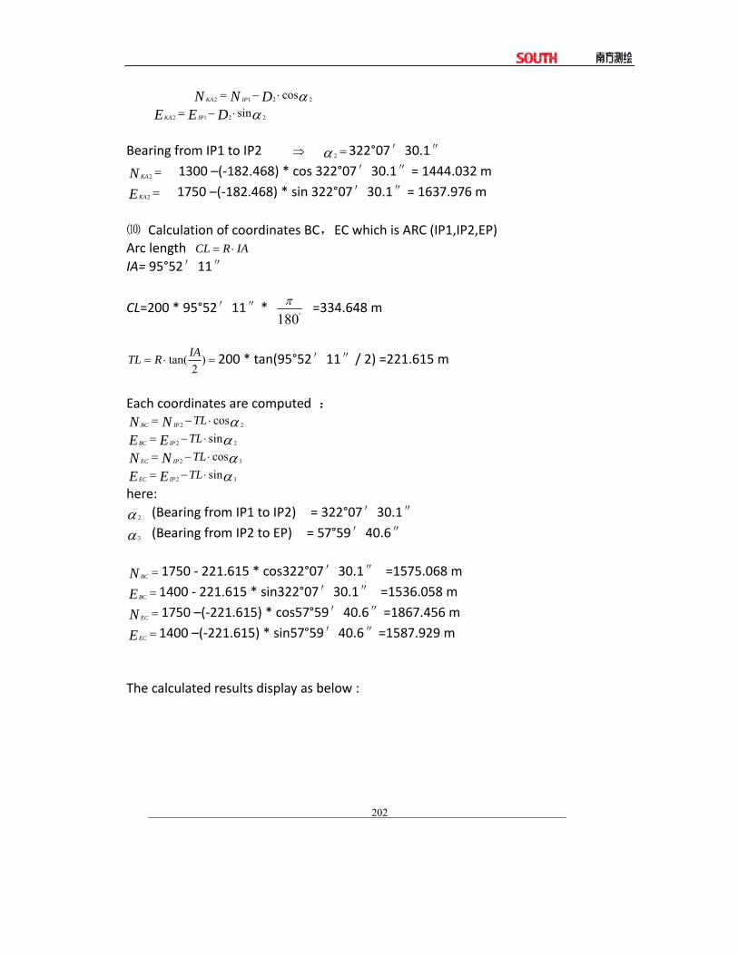
202
α 2212 cos⋅−= DNN IPKA α 2212 sin⋅−= DEE IPKA Bearing from IP1 to IP2 ⇒ =α 2 322°07′30.1″
=N KA2 1300 –(‐182.468) * cos 322°07′30.1″= 1444.032 m =EKA2 1750 –(‐182.468) * sin 322°07′30.1″= 1637.976 m
⑽ Calculation of coordinates BC,EC which is ARC (IP1,IP2,EP) Arc length IARCL ⋅= IA= 95°52′11″
CL=200 * 95°52′11″* 180o
π =334.648 m
=⋅= )2
tan( IARTL 200 * tan(95°52′11″/ 2) =221.615 m
Each coordinates are computed :
α 22 cos⋅−= TLNN IPBC α 22 sin⋅−= TLEE IPBC α 32 cos⋅−= TLNN IPEC α 32 sin⋅−= TLEE IPEC
here:
α 2 (Bearing from IP1 to IP2) = 322°07′30.1″
α 3 (Bearing from IP2 to EP) = 57°59′40.6″
=N BC 1750 ‐ 221.615 * cos322°07′30.1″ =1575.068 m =EBC 1400 ‐ 221.615 * sin322°07′30.1″ =1536.058 m =N EC 1750 –(‐221.615) * cos57°59′40.6″=1867.456 m =EEC 1400 –(‐221.615) * sin57°59′40.6″=1587.929 m
The calculated results display as below :

203
The coordinates and the distance are calculated as below : Compute the length of straight line Straight line
BP∙KA1= 543.545)1050553.1574()000.1100872.1249( 22=+ −− m
straight line KA2∙BC 005.166)976.1637058.1536()032.1444068.1575( 22 =+= −− m
straight line
EC∙EP 084.250)929.15871800()456.18672000( 22 =+= −− m
Start point coordinate (BP) N 1100.000 m E 1050.000 m straight line ( between BP and KA1 ) Bearing 74°03′16.6″ Distance 545.543 m Transition clothoid (between KA1 and KE1) Radius ‐100 m (“‐”sign is turn left curve toward the end point ) Length 64 m ARC (between KE1 and KE2) Radius ‐100 m (“‐” sign is turn left curve toward the end point)

204
Length 131.354 m Transition (Between KE2 and KA2) Radius ‐100 m (“‐” sign is turn left curve toward the end point) Length 64 m Straight line (between KA2 and BC) Bearing 322°07′30.1″ Distance 166.004 m Arc (between BC and EC) Radius 200 (without sign is turn right curve toward the end point) Length 334.648 m Straight line (between EC and EP) Bearing 57°59′40.6″ Distance 250.084 m

205
Technical Specification Distance Measure Part
Type NTS‐962R NTS‐965 R Distance Measurement Max distance (Good weather)
Single prism 5.0Km 5.0Km None prism
300m 300m
Digisplay Max:9999999.999 m Min:1 mm
Precision With prism :2+2ppm Without prism:5+3ppm
Measure time Fine:2s、Quick measure:1.2s、 Track:0.6s
Atmospheric correction
Auto correction
Reflection prism correction
Auto correction
Angle Measurement Measuring method Absolute code Raster diameter 79mm Min display unit 1”/ 5”Selectable Accuracy 2” 5” Detection method Horizontal: Dual
Vertical : Dual Telescope Image Erect Tube length 154mm Effective aperture 45mm,(EDM:50mm) Magnification 30× Field of view 1°30’ Minimum focusing distance
1m
Resolving power 3” Auto Compensator System Dual axis Liquid‐electric Work range ±3’ Accuracy 1”
Vial
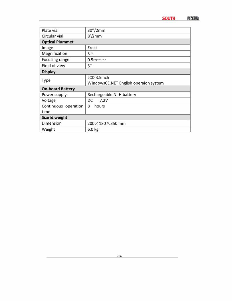
206
Plate vial 30”/2mm Circular vial 8’/2mm Optical Plummet Image Erect Magnification 3× Focusing range 0.5m~∞ Field of view 5° Display
Type LCD 3.5inch WindowsCE.NET English operaion system
On‐board Battery Power supply Rechargeable Ni‐H battery Voltage DC 7.2V Continuous operation time
8 hours
Size & weight Dimension 200×180×350 mm Weight 6.0 kg