Operation IceBridge sea ice freeboard, snow depth, and thickness

data products manual, version 2 processing

Nathan Kurtz and Jeremy Harbeck

1 Overview

The purpose of this document is to describe the retrieval of geophysical data products from the level 1

Operation IceBridge instrument data which can then be used by those wishing to engage in more specialized

research. The document describes the retrieval of three important fundamental sea ice properties from the

IceBridge data set: 1) sea ice freeboard, 2) snow depth, and 3) sea ice thickness. The known limitations

and uncertainties of the derived IceBridge geophysical data products are discussed along with the various

input and output parameters. The primary IceBridge data sets which were used in the retrievals are the

University of Kansas’ snow radar (Leuschen, 2009), the Digital Mapping System (DMS) aerial photography

(Dominguez, 2009), the Continuous Airborne Mapping By Optical Translator (CAMBOT) (Krabill, 2009),

and the Airborne Topographic Mapper (ATM) laser altimeter (Krabill, 2009). The data sets and steps of

the production procedure are illustrated in Figure 1.

The IceBridge data set has and will continue evolving in time as instrument changes are made to improve

the quality of retrievals from the instrument data. A detailed documentation of the baseline processing steps

and justifications for parameter retrieval is provided in Kurtz et al., [2013], while this document outlines the

updated version 2 processing effort which corrects errors in the previous data set and also utilizes improved

techniques for more accurate determination of sea ice thickness. Sections 2-6 provide an up-to-date description

of the primary processing method, while Section 7 lists changes and their associated justifications which were

1

Figure 1: Organization flow chart of sea ice products.

implemented between the version 1 and version 2 data sets. Individual flight specific details are documented

in the appendix.

2 Retrieval of sea ice freeboard

2.1 Freeboard and sea surface height parameters

The primary product given by laser altimeters is the surface elevation referenced to an ellipsoid, he. However,

the more geophysically useful parameter we wish to retrieve from this product is the height of the snow plus

ice surface above sea level, termed the freeboard, fb. The conversion of elevation data into sea ice freeboard is

accomplished by subtracting out the instantaneous sea surface height hssh from each elevation measurement:

fb = he − hssh (1)

2

Parameter Data sourcehgeoid EGM08 geoidhdynamic DTU10 Mean Sea Surfacehocean TPXO8.0hload TPXO8.0hearth ATM processing (see text)hpressure MOG2D model, Meteo France

Table 1: Sea surface height data sources.

The instantaneous sea surface height at a given point in space and time can be written as (Chelton et al.,

2001):

hssh = hgeoid + hdynamic + htides + hpressure (2)

where hgeoid is the geoid, htides is the contribution of tidal forces, hpressure is the effect of atmospheric

pressure loading, and hdynamic is the dynamic topography of the ocean surface. As a first step, we estimate

the instantaneous sea surface height along the flight tracks through modeled estimates for the hgeoid, hdynamic,

htides, and hpressure terms. Data sources used in the initial estimation of the sea surface height terms are

shown in Table 1.

The hgeoid component is taken from the EGM08 geoid, while the hdynamic component is estimated from the

1 minute by 1 minute DTU10 Mean Sea Surface data set (Andersen and Knudsen, 2009).

The htides component can be further decomposed into 4 terms:

htides = hocean + hload + hearth + hpole (3)

where hocean is the ocean tide, hload is the load tide, hearth is the solid earth tide, and hpole is the pole tide.

The ATM elevation product is provided in the ITRF standard tide-free system where the solid earth tide

has been removed. A standard latitude dependent correction for the permanent earth tide, hpermtide−corr,

is applied to the data used here to place the data in a mean tide system relative to the WGS84 ellipsoid.

The pole tide is a small amplitude (< ~ 2 cm), long wavelength tide component caused by oscillations in the

3

Earth’s rotation axis, it has not been included with this data set since its impact on freeboard determination

should be minimal. The TPXO8.0 tide model is used to estimate the hocean and hload components (Egbert

and Erofeeva, 2002).

The classic expression for the hpressure component can be rewritten as:

hpressure = ∆P/(ρwg) (4)

where ∆P is the difference between the surface air pressure at the local point from the instantaneous mean

surface air pressure over the ocean, ρw = 1024 kgm3 the density of sea water, and g = 9.8 m

s2 the gravitational

acceleration. However, this represents only the time-invariant response of the sea surface height, we therefore

use a dynamic atmospheric correction term taken from the MOG2Dmodel (Carrère and Lyard, 2003) provided

by Meteo France.

2.2 Sea surface height and freeboard determination

The previously described sea surface height parameters cannot be modeled with sufficient accuracy for the

useful retrieval of freeboard given that centimeter level accuracy of the sea surface height is necessary for

sea ice thickness studies. A combination of the modeled sea surface height with local sea surface height

observations is thus required to achieve the desired centimeter level accuracy for the freeboard retrievals.

A first step in the freeboard retrieval process is an initial removal of the modeled parameters affecting sea

surface height from he, resulting in a corrected elevation hcorr:

hcorr = he − (htides + hgeoid + hdynamic + hpressure) (5)

with the resulting freeboard then calculated as:

fb = hcorr − zssh (6)

4

where zssh is the locally determined sea surface elevation with respect to the hcorr elevation data set, the

determination of zssh at each point along the flight track follows from the retrieval of individual sea surface

height observations described in detail below.

A set of sea surface elevation estimates, htp, are first found through extraction of the hcorr elevation data

identified over leads in the IceBridge visible imagery data sets. For all but the Arctic 2009 data set (and other

specific cases noted in the appendix), an automated lead detection algorithm called Sea Ice Lead Detection

Algorithm using Minimal Signal (SILDAMS) (Onana et al., 2013) which utilizes the geolocated IceBridge

DMS imagery is used. SILDAMS applies a minimal signal transformation on DMS pixel brightness values to

carry out a localization around low pixel intensities which correspond to lead areas. The transformed outputs

are within a uniform dynamic variability over the set of numbers from [0, 1] for a variety of input image pixel

intensities. This allows specified thresholding of the transformed outputs to be set for the identification and

classification of three different lead classes corresponding to open water areas, grease ice/nilas, and newly

frozen leads with non-snow-covered grey ice (see Fig. 2). Each of these lead classes has an ice thickness less

than 30 cm (World Meteorological Organization, 1970) and should thus have an elevation to within 3 cm of

the local mean sea level making them suitable for use as sea surface tie points. To account for biases in the use

of thin ice areas as sea surface tie points, we subtracted 0.005 m and 0.02 m of elevation for sea surface height

determination using the ATM data over grease ice/nilas and grey ice, respectively. These values were chosen

to correspond to expected freeboards of snow-free ice types defined by the World Meteorological Organization

nomenclature.

For the 2009 Arctic campaign, leads and ice type were categorized through visual inspection of CAMBOT

images (Krabill, 2009). Visual lead identification, rather than an automated approach using SILDAMS, was

also used due to the complexity of the CAMBOT images caused by failure of the mechanical camera shutter

and uneven image exposure in some portions of the images. The CAMBOT images are taken once every

five seconds along each flight path using a Canon EOS DIGITAL REBEL XTi camera. The images are

time tagged and the geolocation of the center point, height of the aircraft above the surface, and aircraft

heading are provided from the aircraft trajectory information based on the time tag. We have measured the

angular resolution of the camera images using pictures of three distinct buildings over the Thule Airforce

5

Figure 2: Example DMS image of sea ice with results from the SILDAMS algorithm displaying the abilityto distinguish between a) open water leads b) nilas and grease ice and c) non-snow-covered grey-white ice.Overlain ATM elevation measurements (colored circles) are also shown. The colors correspond to heightvariations in the ATM data with cool colors (e.g. blue and purple) having a low elevation and warm colors(e.g. yellow and red) having a high elevation.

6

Base collected in 2009 with CAMBOT system and 2010 with the DMS system. The spatial size of the

buildings were assumed to be unchanging and measured with the DMS imagery in 2010, combined with the

known aircraft altitude from the CAMBOT system these same buildings were used to determine the angular

resolution of the CAMBOT system to be 58.12◦ x 40.71◦. The aircraft altitude and angular resolution were

used to determine the pixel size for each CAMBOT image in the 2009 data set. The pixel size was combined

with the image center point location, aircraft heading, and a standard coordinate rotation to geolocate the

pixels of each CAMBOT image. However, the time tagging procedure for the CAMBOT data set was found

to be typically valid only to within ±1 second, which introduces geolocation errors for each image. To refine

the geolocation of each image, we have constructed software to manually align each CAMBOT image. The

software overlays the more accurately geolocated ATM elevation data (accurate to better than 1 m, Schenk

et al., 1999) onto each image, and then allows the operator to adjust the CAMBOT geolocation by manually

changing the geolocation of the center point of each image. This was done until topographic features such as

ridges and leads were found to match between the images and ATM data, see Figure 3 for an example image

showing a manually aligned CAMBOT image with ATM data overlain. By matching the location of the leads

in the visible imagery with those of the ATM hcorr elevations, the local sea surface elevation and freeboard of

each ATM elevation point was retrieved in the same manner as leads identified with SILDAMS. Bias removal

due to the use of thin ice types as sea surface reference points was done in the same manner as above using

the SILDAMS output. The albedo dependence of ice type with thickness was found to impact the ATM data,

very smooth specularly reflecting surfaces such as open water and thin ice covered leads caused a large loss

in the number of returns from the ATM wide scan system. Non-snow covered thick grey-white ice had the

largest number of returns which approached the sampling density of the surrounding snow-covered sea ice.

Thus, even if leads are present in an area, the amount of sea surface elevation estimates may be much more

limited in number than those from an equivalent area of returns over sea ice. In later campaigns, the smaller

incidence angle of the ATM narrow scan instrument largely mitigates this issue.

The spatial resolutions of the ATM laser footprint and lead detection steps are ∼1 m for the nominal flight

altitude (460 m) of the IceBridge data set. To account for geolocation errors as well as the presence of mixed

lead/sea ice data within the ATM returns, the requirement of a minimum 1 m lead buffer was set for each

ATM return over a lead for it to be used as a sea surface estimate. This is necessary because mixed lead/sea

7

Figure 3: Example manually aligned CAMBOT image of sea ice with overlain ATM elevation measurements(colored circles) also shown. The colors correspond to height variations in the ATM data with cool colors(e.g. blue and purple) having a low elevation and warm colors (e.g. yellow and red) having a high elevation.

8

ice returns are prevalent due to the highly backscattering sea ice portion of the surface; as such, laser returns

near the edge of a lead are not representative of the actual sea surface elevation but rather that of the sea

ice within the laser footprint. Thus, the set of sea surface elevation estimates, htp, are taken from the hcorr

elevation data set where leads are found, and the lead is found to extend at least 1 m in all directions beyond

the center point.

Within a given area, h̄tp can be found from the set of sea surface elevation estimates, htp which were

determined using the combined ATM and visible imagery lead detection method described previously. h̄tp

is calculated using the following procedure: All values of htp within ±250 m from the center point are first

combined into a histogram with a 2 cm bin size. A value of ±250 m has been chosen to span the width of

an individual DMS or CAMBOT image. At minimum, we expect the local sea surface height to be constant

over a length scale corresponding to the first mode baroclinic Rossby radius of deformation which is on the

order of 10 km for latitudes greater than 60◦ (Chelton et al., 1998). The Rossby radius is associated with

the length scale at which oceanic eddies form, these eddies can cause local inhomogeneities in the sea surface

height. An analysis of histograms of ATM elevations over known flat surfaces, including separate cases with

open water and flat snow-covered sea ice (e.g. Farrell et al., 2012), showed that the elevation distributions

are Gaussian in shape with a minimum standard deviation of ∼5 cm. For large leads during the 2012 and

2013 Arctic campaigns, the standard deviation of the ATM narrow swath instrument was ~3-5 cm which

is of higher precision than the wide scan instrument which was used exclusively in the early part of the

mission. We thus ideally expect the distribution of all htp points within the length scale defined by the

Rossby radius to be similar in shape and width. However, a variety of error sources ranging from geolocation

errors, misidentification of lead returns in the visible imagery, and errors in the hssh data sources lead to

deviations from this ideal scenario. These errors also preclude the use of the mean value of htp and standard

error analysis techniques from being used to determine h̄tp and its associated error. The misidentification of

lead returns within the combined ATM and photography data causes the largest impact which, when present,

can be seen as the presence of secondary and higher modes in the histogram of the htp points. In determining

h̄tp, we wish to use the points corresponding to the mode with the lowest elevation. This is accomplished

through the use of the centroid of a Gaussian fit function to the histogram of htp. The following conditions

9

have been imposed to determine whether the fitted Gaussian function is of a high enough quality for use in

determining h̄tp:

σfit ≤ 0.11m

χ2 < 0.015

N ≥ 40

(7)

where σfit is the standard deviation of the Gaussian fit, χ2 is the reduced chi-square goodness-of-fit, and N is

the number of htp points used to construct the histogram for the Gaussian fit. In cases where a multi-modal

distribution of htp is observed, the above parameters will not be satisfied for the initial Gaussian fit. If this

occurs, an iteration is then performed by discarding the largest htp elevation point in the set, performing

another Gaussian fit, and retesting the fit parameters. The iteration is repeated until the conditions for

the fit parameters are satisfied, at which point h̄tp is subsequently determined. If the conditions for the fit

parameters are not met, then the sea surface height and freeboard are not calculated. See Figure 4(a) for an

example of a case where the initial Gaussian fit parameters were satisfied on the first iteration, and Figure

4(b) for an example case of a multimodal distribution where the iteration produced a fit of the first mode

only.

10

Figure 4: a) Gaussian fit to sea surface height data points which passed the quality requirements with noiteration required. b) Gaussian fit to sea surface height data points which passed the quality requirementsafter iterative removal of data points.

The previously described procedure produces a set of discrete sea surface height observations along the flight

track. The availability of these sea surface height observations was found to be inconsistently available along

each flight track due to ice conditions, in particular, few leads were found to occur in the compact multiyear

ice areas of the Arctic. This creates uncertainties in the retrieval of freeboard since the quality of the sea

surface height observations decreases with distance due to inaccuracies in the removal of the modeled sea

surface height parameters shown in equation 2. Therefore, to construct the freeboard profiles along the

flight track and determine the uncertainty of each data point (which is inherently variable along the flight

path due to uneven lead spacing), the sea surface height along the full flight track was interpolated using

11

an ordinary kriging approach (e.g. Cressie, 1993). Since the sea surface height field is non-isotropic and

non-homogeneous, we perform the interpolations over 200 km segments of each flight line and assume that

the covariance of the sea surface height field is a homogeneous function of distance. Using these assumptions,

the interpolation is then performed by minimizing the error variance of the interpolated vector of sea surface

heights along the flight path. Briefly, this is done by solving the equation

zssh = WTzo (8)

where zssh is the interpolated sea surface height at a specific point along the flight path, zo is the vector of

observed sea surface height observations comprised of the set of h̄tp values calculated for each flight segment,

and W is the weight vector. W is found by solving

W1...

Wn

µ

=

1

C...

1

1 . . . 1 0

−1

Co1...

Con

1

(9)

W =

W1...

Wn

(10)

where C is the covariance matrix and Coy is the covariance between the interpolation point y, and the

observation point o. The elements of the covariance matrix are assumed to be a homogeneous function of

distance which is modeled as a Gaussian process with the respective elements taken to be

Cxy = ε2ssh + σ2z

(1− e−

d2xy

L2

)(11)

12

and

Con =[ε2ssh + σ2

z

(1− e−

d2onL2

)]e(−donLm

) (12)

where dxy is the distance between points x and y, don is the distance between observation points o and n,

L is the correlation length of the sea surface height observations (zo) along the flight segment, Lm is the

correlation length of the sea surface height measurements, σz is the standard deviation of the sea surface

height observations, and εssh is the uncertainty of the sea surface height observations. When a large number

of closely spaced leads are present (which is typical in the Antarctic region) problems arise in the matrix

inversion to determine the weights used in the sea surface height interpolation algorithm. To mitigate this,

the h̄tp observations are averaged to 5 km to avoid singularities during the matrix inversion process when a

potentially ill-conditioned matrix is detected in processing. Lastly, the method of Deutsch, [1996] is applied

to correct for any non-physical negative weights and ensure unbiasedness.

From the previously described method for determining h̄tp containing at least 40 observations and a standard

deviation of 0.11 m, the uncertainty for the sea surface height observations should theoretically be better

than 0.11/√

40 = 0.017 m. However, additional errors such as unresolved aircraft pitch and roll errors set

will likely make this number higher since each sea surface height elevation data point, htp, is not statistically

independent. We take εssh = 0.058/(∑ni=1 exp(−

d2oi

L2 )).5 meters (with a maximum value of εssh = 0.058

m) based on observations from the 2009 Arctic data set where 0.058 m is the standard deviation of the

differences of all h̄tp measurements within ±5 km (the Rossby radius where we expect the sea surface height

to be constant) of each individually observed lead. Using a length scale smaller than ±5 km did not change

the maximum value of εssh = 0.058 m suggesting that this is the minimum uncertainty of a single sea surface

height observation due to instrumental limitations. The higher precision of the narrow scan instrument will

likely lead to a lower value for εssh, but this has not been implemented at this time. Lastly, the sea ice

freeboard is then determined by combining equations 6 and 8. The uncertainty in sea surface height and

therefore freeboard at each point is given by

13

σssh =

(W1 · · · Wn µ

)

Co1...

Con

1

12

(13)

Qualitatively, the local sea surface height is determined by weighting the sea surface height observations as

a function of distance, with nearby h̄tp points receiving the largest weight. The uncertainty decreases as the

number of sea surface observations increases and the distance from each sea surface observation decreases,

approaching σssh = 0.058√N

meters in an area with many nearby sea surface height observations. The uncertainty

approaches that of the background sea surface height field standard deviation, σz, as the distance from the

nearest sea surface height observation becomes large.

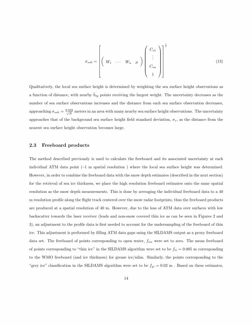
2.3 Freeboard products

The method described previously is used to calculate the freeboard and its associated uncertainty at each

individual ATM data point (~1 m spatial resolution ) where the local sea surface height was determined.

However, in order to combine the freeboard data with the snow depth estimates (described in the next section)

for the retrieval of sea ice thickness, we place the high resolution freeboard estimates onto the same spatial

resolution as the snow depth measurements. This is done by averaging the individual freeboard data to a 40

m resolution profile along the flight track centered over the snow radar footprints, thus the freeboard products

are produced at a spatial resolution of 40 m. However, due to the loss of ATM data over surfaces with low

backscatter towards the laser receiver (leads and non-snow covered thin ice as can be seen in Figures 2 and

3), an adjustment to the profile data is first needed to account for the undersampling of the freeboard of thin

ice. This adjustment is performed by filling ATM data gaps using the SILDAMS output as a proxy freeboard

data set. The freeboard of points corresponding to open water, fow were set to zero. The mean freeboard

of points corresponding to “thin ice” in the SILDAMS algorithm were set to be fti = 0.005 m corresponding

to the WMO freeboard (and ice thickness) for grease ice/nilas. Similarly, the points corresponding to the

“grey ice” classification in the SILDAMS algorithm were set to be fgi = 0.02 m . Based on these estimates,

14

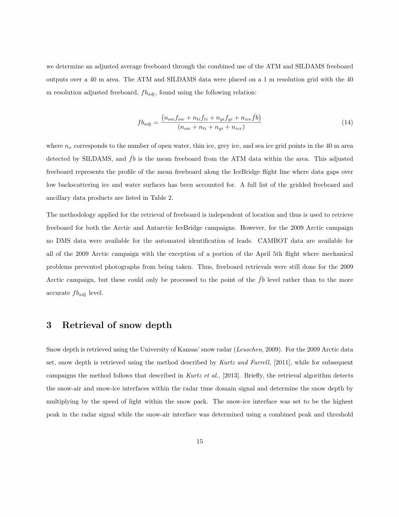
we determine an adjusted average freeboard through the combined use of the ATM and SILDAMS freeboard

outputs over a 40 m area. The ATM and SILDAMS data were placed on a 1 m resolution grid with the 40

m resolution adjusted freeboard, fbadj , found using the following relation:

fbadj =(nowfow + ntifti + ngifgi + nicef̄ b

)(now + nti + ngi + nice)

(14)

where nx corresponds to the number of open water, thin ice, grey ice, and sea ice grid points in the 40 m area

detected by SILDAMS, and f̄ b is the mean freeboard from the ATM data within the area. This adjusted

freeboard represents the profile of the mean freeboard along the IceBridge flight line where data gaps over

low backscattering ice and water surfaces has been accounted for. A full list of the gridded freeboard and

ancillary data products are listed in Table 2.

The methodology applied for the retrieval of freeboard is independent of location and thus is used to retrieve

freeboard for both the Arctic and Antarctic IceBridge campaigns. However, for the 2009 Arctic campaign

no DMS data were available for the automated identification of leads. CAMBOT data are available for

all of the 2009 Arctic campaign with the exception of a portion of the April 5th flight where mechanical

problems prevented photographs from being taken. Thus, freeboard retrievals were still done for the 2009

Arctic campaign, but these could only be processed to the point of the f̄ b level rather than to the more

accurate fbadj level.

3 Retrieval of snow depth

Snow depth is retrieved using the University of Kansas’ snow radar (Leuschen, 2009). For the 2009 Arctic data

set, snow depth is retrieved using the method described by Kurtz and Farrell, [2011], while for subsequent

campaigns the method follows that described in Kurtz et al., [2013]. Briefly, the retrieval algorithm detects

the snow-air and snow-ice interfaces within the radar time domain signal and determine the snow depth by

multiplying by the speed of light within the snow pack. The snow-ice interface was set to be the highest

peak in the radar signal while the snow-air interface was determined using a combined peak and threshold

15

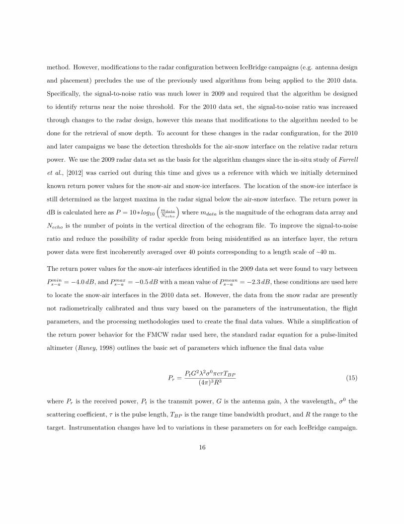
method. However, modifications to the radar configuration between IceBridge campaigns (e.g. antenna design

and placement) precludes the use of the previously used algorithms from being applied to the 2010 data.

Specifically, the signal-to-noise ratio was much lower in 2009 and required that the algorithm be designed

to identify returns near the noise threshold. For the 2010 data set, the signal-to-noise ratio was increased

through changes to the radar design, however this means that modifications to the algorithm needed to be

done for the retrieval of snow depth. To account for these changes in the radar configuration, for the 2010

and later campaigns we base the detection thresholds for the air-snow interface on the relative radar return

power. We use the 2009 radar data set as the basis for the algorithm changes since the in-situ study of Farrell

et al., [2012] was carried out during this time and gives us a reference with which we initially determined

known return power values for the snow-air and snow-ice interfaces. The location of the snow-ice interface is

still determined as the largest maxima in the radar signal below the air-snow interface. The return power in

dB is calculated here as P = 10∗ log10(mdataNecho

)where mdata is the magnitude of the echogram data array and

Necho is the number of points in the vertical direction of the echogram file. To improve the signal-to-noise

ratio and reduce the possibility of radar speckle from being misidentified as an interface layer, the return

power data were first incoherently averaged over 40 points corresponding to a length scale of ~40 m.

The return power values for the snow-air interfaces identified in the 2009 data set were found to vary between

Pmins−a = −4.0 dB, and Pmaxs−a = −0.5 dB with a mean value of Pmeans−a = −2.3 dB, these conditions are used here

to locate the snow-air interfaces in the 2010 data set. However, the data from the snow radar are presently

not radiometrically calibrated and thus vary based on the parameters of the instrumentation, the flight

parameters, and the processing methodologies used to create the final data values. While a simplification of

the return power behavior for the FMCW radar used here, the standard radar equation for a pulse-limited

altimeter (Raney, 1998) outlines the basic set of parameters which influence the final data value

Pr = PtG2λ2σ0πcτTBP(4π)3R3 (15)

where Pr is the received power, Pt is the transmit power, G is the antenna gain, λ the wavelength„ σ0 the

scattering coefficient, τ is the pulse length, TBP is the range time bandwidth product, and R the range to the

target. Instrumentation changes have led to variations in these parameters on for each IceBridge campaign.

16

Flight considerations also play a role, for example R is generally equal to the nominal IceBridge flight altitude

of 460 m, but can be as low as 240 m as the aircraft altitude is varied to fly under clouds which negatively

impact the laser altimetry data. A calibration adjustment for each individual radar echogram is therefore

necessary to determine the final threshold power range where we expect the snow-air interface to be located.

First, we define scale, m, and offset, b, parameters which are determined for each echogram by simultaneously

solving

y1 = mx1 + b (16)

y2 = mx2 + b (17)

where y1 = 2.25 dB which is the average power of the snow-ice interface observed in the 2009 Arctic data set,

x1 is the average power of the snow-ice interface for the desired radar echogram, y2 = −5.0 dB which is the

average power of the first 100 bins located at least 5 m above the point of maximum power in the 2009 Arctic

data set, and x2 is the average power of the first 100 bins located at least 5 m above the point of maximum

power for the desired radar echogram. We here define the maximum power of the adjusted snow-air interface

to be P̂maxs−a = mPmaxs−a + b, similarly the minimum power for the adjusted snow-air interface is defined to be

P̂mins−a = mPmins−a + b. These conditions determine the region of the radar return where we expect the snow-air

interface to be located. The search for the snow-air interface thus occurs when the return power level, Ps−a,

for the snow-air interface satisfies the following requirements:

Ps−a ≥ P̂mins−a (18)

Ps−a ≥ P̂mins−a (19)

17

where Ps−a is the mean power in the six range bins that follow the P̂mins−a . Once these conditions are satisfied

the snow-air interface is defined following the observations described by Farrell et al., [2012] to be either the

location of the first local maxima in the return or the leading edge of the radar signal. The snow-air interface

is thus defined here as the first point where one of the following conditions is satisfied:

1. The leading edge of the radar return from the snow-air interface is found. The leading edge is defined here

as the point where the radar return power begins to continuously increase (i.e. ∂P∂x > 0) until the maximum

snow-air interface power, P̂maxs−a is reached.

2. If a local maxima occurs greater than mPmeans−a + b and σ above the adjacent points (to eliminate random

noise from being misidentified as a maxima), where σ is the standard deviation of the radar noise level, then

this point is chose as the snow-air interface location.

An iteration of the above method is then performed by rescaling the threshold power values: y1 is set

equal to the mean echogram power for the snow-air interface and y2 = Pmeans−a . The first iteration provides an

approximation for the parameters m and b by scaling the return power values by the snow-ice interface power

and the radar noise, however changes to the snow radar system have reduced the noise level in successive

campaigns. The second iteration scales the return power values to the snow-air interface allowing for more

accurate estimates of m and b to be made.

The snow depth is then found by differencing the snow-air and snow-ice interfaces in the time domain and

multiplying this difference by the speed of light within the snow pack, csnow. The speed of light in the snow

pack was taken to follow the relation between snow density and dielectric constant given by Tiuri et al. [1984]

as

εd = 1 + 2ρs (20)

csnow = c√εd

(21)

18

where c is the speed of light in vacuum and ρs is the snow density (in gcm3 ). The snow density was taken

to be 320 kgm3 following the climatological mean snow density of Warren et al., [1999]. Once the snow-air

and snow-ice interfaces were identified, we applied a locally weighted robust linear regression at a 40 m

length scale to reduce the impact of outliers in the final determination of the snow-air and snow-ice interface

locations. This effectively reduces the resolution of the retrieved snow depths to 40 m.

As described in Kurtz and Farrell, [2011], the behavior of the radar over leads and the apex of steep pressure

ridges must also be accounted for in the snow depth retrieval method. Lead areas were flagged using the

method described in Kurtz and Farrell, [2011] and the snow depth was set to zero to correspond to the

negligible snow cover on open water and newly frozen leads. We also discard data where the signal is too

low for the retrieval of snow depth. Based on the analysis of coincident laser data from the ATM to identify

ridge locations, the conditions for discarding the data due to insufficient signal strength were set to be:

Ps−i ≥ −1.5m+ b dB (22)

Ps−i ≥ −1.5m+ b dB (23)

where Ps−i is the mean power in the three range bins that follow the snow-ice interface. Discarding of

data due to insufficient signal strength occurred for 16% of the snow depth observations for the 2009 Arctic

campaign, but will be variable for each campaign due to flight line and instrumentation differences.

An additional quality control step for the retrieved snow depths is also necessary to discard data collected

when warm surface temperatures are present. Kurtz and Farrell, [2011] found that warm surface temperatures

led to anomalously low snow depth values due to the changing dielectric properties of the snow pack. Similar

to the study of Kurtz and Farrell, [2011], we discard data when the surface temperature is greater than

-5 ◦C. When available, the surface temperature is determined from the IceBridge KT-19 infrared radiation

pyrometer data set (Shetter et al., 2010). When instrumental observations are unavailable, we use the

thermodynamic sea ice model of Kurtz et al., [2011] forced with ECMWF meteorological data to determine

the surface temperature.

19

The snow depth retrieval method outlined here is essentially empirical, an updated method which utilizes

known physics of the radar return is underway. It will be evaluated and included in a future version of the

data product if it shows an improvement over the current method.

4 Sea ice thickness

4.1 Thickness determination and spatial resolution

Sea ice thickness, hi, is calculated using the previously described freeboard and snow depth data sets and

the hydrostatic balance equation:

hi = ρwρw − ρi

fbadj −ρw − ρsρw − ρi

hs (24)

where fbadj is the freeboard,hs is the snow depth, ρw is the density of sea water, ρi is the density of sea ice,

and ρs is the density of snow. ρw and ρi are taken to be 1024 kgm3 and 915 kg

m3 which are derived from the

result of field measurements summarized by Wadhams et al. [1992]. ρs is taken to be 320 kgm3 following the

climatological values compiled by Warren et al. [1999].

4.2 Error analysis

The error in the sea ice thickness retrieval (excluding the negligible contribution of errors due to variations

in sea water density as shown by Kwok and Cunningham, 2008) can be written as

σhi =

( ρwρw − ρi

)2σ2hf

+(ρs − ρwρw − ρi

)2σ2hs +

(hs (ρs − ρw) + hfρw

(ρw − ρi)2

)2

σ2ρi +

(hs

ρw − ρi

)2σ2ρs

12

(25)

where σhi , σhf , σhs , σρs , and σρi are the uncertainties of the ice thickness, freeboard, snow depth, and

densities of snow and ice, respectively. Density uncertainties are taken from previous in-situ measurements

20

described in the literature: σρs is estimated to be 100 kg/m3 based on the variability of ρs in the climatology

of Warren et al. [1999], σρi is estimated here to be 10 kg/m3 which represents the expected range of densities

for sea ice between 0.3 and 3 m thick (Kovacs, 1996). The uncertainty in the freeboard retrieval, σhf , is

variable along the flight path as described in Section 2. The snow depth uncertainty is not well known at this

time. Uncertainty in the snow depth occurs due to a variety of factors including the finite range resolution of

the radar, density uncertainties, and uncertainty in the detection of the snow-air and snow-ice interfaces. For

the purposes of this study, we estimate the uncertainty using the difference between the IceBridge data and

in-situ snow depth described in the study by Farrell et al., [2012]. The mean difference between the survey

and IceBridge data set was 0.8 cm, and there were 50 observations (40 m for each observation over a 2 km

survey line). Assuming the method is unbiased the error is calculated as σhs0.8 ∗√

50 = 5.7 cm, a recent

study by Webster et al., [2014] found an RMSE of 5.8 cm in comparison to in-situ data. However, we await

further refinement of this uncertainty value with the addition of future in-situ comparisons. The uncertainty

in ice thickness is then calculated using equation 25, with the uncertainties for the variable described above.

The sea ice thickness uncertainty is thus a variable quantity, in particular due to the variable uncertainty in

the freeboard retrievals.

5 Data products description

The full suite of data products and ancillary data sets are listed in Table 2. Additional ancillary data have

been included for further analysis of the IceBridge data sets. These include the surface roughness, transmit

and received signal strength of the ATM, and the KT19 surface and internal temperatures. A flag for ice

type is also included for the Arctic region, the ice type flag data are taken from the nearest grid data on

ice type from the Norwegian Met. Service OSI SAF system (http://www.osi-saf.org/). The gridded data

products contain invalid data which are set to a value of -999, additionally, ice type data with a confidence

level less than 50% were also set to -999.

21

Name Symbol in text Description Units

Profile data

Latitude - Latitude of the center grid point Degrees

Longitude - Longitude of the center grid point Degrees

Mean freeboard f̄b Mean freeboard (40 m resolution) of the ATM data only m

Adjusted mean freeboard fbadj Mean freeboard (40 m resolution) from the combined ATM-DMS data set m

ATM points natm Number of ATM points in the 40 m grid #

Percentage open water pow Percentage of open water in the 40 m grid %

Percentage thin ice pti Percentage of thin ice in the 40 m grid %

Percentage grey ice pgi Percentage of grey ice in the 40 m grid %

Freeboard uncertainty σssh Uncertainty in the derived freeboard m

Mean snow depth hs Mean snow depth (40 m resolution) from the snow radar data set m

Snow depth uncertainty σhs Uncertainty in the derived snow depth m

Sea ice thickness hi Mean sea ice thickness (40 m resolution) m

Sea ice thickness uncertainty σhi Uncertainty in the derived sea ice thickness m

Surface roughness - Standard deviation of the ATM elevation points in the 40 m grid m

Transmit energy - Mean transmit signal strength (40 m resolution) of the ATM data -Received energy - Mean receive signal strength (40 m resolution) of the ATM data -

Low energy correction - Correction added to the ATM elevation data for low signal strength m

Scan angle correction - Correction added to the ATM elevation data for scan angle biases m

Snow-air interface - Height of radar derived snow-air interface relative to the WGS84 ellipsoid m

Snow-ice interface - Height of radar derived snow-ice interface relative to the WGS84 ellipsoid m

Ice type flag - Flag for ice type, 0: first year ice, 1: multiyear ice -

Ancillary data

Corrected elevation hcorr Elevation with the modeled sea surface height parameters removed m

Elevation he Original ATM elevation m

Date - Date of measurement in YYYYMMDD

Elapsed time - Time from start of day of the flight, in UTC Seconds

Ellipsoid correction he Conversion factor between the WGS-84 ellipsoid and the Topex/Poseidon ellipsoid m

Atmospheric loading hpressure Atmospheric pressure loading term for the sea surface height m

Mean sea surface - DTU10 mean sea surface height equal to hgeoid + hdynamic m

Ocean tide hocean Ocean tide term for the sea surface height m

Load tide hload Load tide term for the sea surface height m

Permanent tide correction hpermtide−corr Tide correction term used to place the data in the mean tide system m

Total tides htides Sum of the ocean, load, and earth tide correction terms m

Sea surface height zssh Local sea surface elevation with the ocean, load, and earth tide correction terms applied m

SSH number nssh Number of ATM points used to determine the nearest h̄tp data point #

SSH standard deviation σssh Standard deviation of the Gaussian fit used to determine the nearest h̄tp point m

SSH difference - Difference between centroids of the first and final Gaussian fits used to determine h̄tp m

SSH elapsed time - Elapsed time since the last sea surface tie point was encountered Seconds

SSH tie point distance - Distance to the nearest sea surface height tie point m

File name - Name of the file from which the laser altimetry data were from

Surface temperature - Surface temperature from the KT19 instrument ◦C

KT19 internal temperature - Internal temperature of the KT19 instrument ◦C

Table 2: Descriptions of the final gridded freeboard, snow depth, and ice thickness output fields and ancillarydata. 22

6 Ancillary data sets and adjustments

6.0.1 KT-19 surface temperature retrievals

A KT-19 infrared pyrometer is present on many of the campaigns to measure surface temperature. The data

are recorded using an averaging rate, ktavg, which has varied between 1-10 Hz for individual campaigns.

At the nominal aircraft speed of vaircraft = 460 km/hr (128 m/s), the averaging length is al = vaircraftktavg

which is one component of determining the footprint size. The two degree instrument field of view yields a

footprint size of fkt = 15 m at the nominal flight altitude of 457 meters. The footprint size of the recorded

measurement is thus al + fkt. The geolocation of the data are referenced to a GPS antenna located near

the KT19 instrument. Meter to decameter level geolocation uncertainties may be present due to the lack

of knowledge of the instrument pointing angle (assumed to be at nadir) as well as timing offsets from the

instrument data system.

The uncertainty in the surface temperature retrievals are calculated following the KT19 product manual as

σkt19 = 0.5 + 0.007∆T (26)

where ∆T is the temperature difference between the target surface and the housing temperature, unmodeled

uncertainties include surface emissivity variations, instrument issues, and atmospheric losses from clouds,

fog, and atmospheric water vapor.

Prior to 2011 the response time setting for the emissivity for the KT-19 instruement was set at 1.0. However,

published values for the emissivity of snow and sea ice are ~0.97, a setting which was adopted for all Arctic

and Antarctic campaigns beginning in 2012. A bias correction can be calculated by integrating Planck’s

law over the wavelength range of the KT19 instrument to determine the total intensity, I1, for the recorded

temperature with emissivity, ε1 = 1 , and the total intensity, I2, with emissivity, ε2 = 0.97:

I1 =λ2�

λ1

ε12hc2

λ51

ehc

λkbT1 − 1dλ (27)

23

I2 =λ2�

λ1

ε22hc2

λ51

ehc

λkbT2 − 1dλ (28)

where λ1 = 9.6x10−6m, λ2 = 11.5x10−6m, h is the Planck constant, c is the speed of light, kb is the Boltz-

mann constant, T1 is the temperature which was recorded using the KT19 sensor, and T2 is the temperature

of the surface with emissivity ε2. This equation does not have a closed form solution and must be solved

numerically. Setting I1 = I2, the equation can be iteratively solved to determine T2. A plot of calculated

values for T2 − T1 for different recorded KT19 temperatures, T1, is shown in Figure 5. A linear fit to the

calculated values to determine the temperature bias is:

T2 − T1 = T1 ∗ 0.01066− 1.263 (29)

Equation 29 was used to correct the recorded KT19 temperature values to coincide with a surface emissivity

of 0.97 for all data reported in the products prior to 2012.

6.0.2 Iceberg filter

The goal of the IceBridge sea ice campaigns is to measure the freeboard and thickness of sea ice. In the

Antarctic region there are a substantial number of icebergs which contaminate the measurements of sea ice.

Since the fundamental goal of the data provided in these products is to provide information on sea ice, we

wish to filter out data which contain icebergs. Since icebergs cast long and dark shadows which can be

mistaken for leads in the lead identification step using SILDAMS, we also wish to filter out these points. The

following steps describe the process whereby the ATM data with iceberg contamination are identified and

removed.

First, an ATM point cloud (anywhere from a small ~200m in length subset to an entire flight) is input into

a function and a structure of two arrays are output. The first array (“iceberg”) contains the index of the

points that are identified as being on the iceberg. The second array contains these iceberg indices, as well as

those points lying within a specified radius from the edge of the iceberg (“shadow”); this additional buffer is

24

Figure 5: Starred points are calculated values for T2 − T1 for different recorded KT19 temperatures, T1. Alinear fit to the data (solid line) which was used to calculate the temperature bias is given in equation 29.

25

an attempt to capture all the points that may be within the reach of a shadow cast from the iceberg. This

“shadow” array is useful in conjunction with additional lead identification methods to differentiate areas

identified as leads that are actual leads from those that are shadows. Tall icebergs with low sun angles often

necessitate a large buffer to be used.

1. Projecting the input data

(a) ATM data is first projected into a polar stereographic projection with a decameter resolution.

(b) Next the projection is translated such that the minimum x and y values are set as zero; all other

x and y values subsequently become positive.

2. Gridding the data

(a) Two empty grids are created, spanning the entire range of x and y values. Grid A will contain the

average value of all the points that fall within each grid square. Grid B will contain the maximum

value of all the points that fall within each grid square.

(b) Each point is then placed into the appropriate grid square based on its projected coordinates.

Grid B values (maximums) are calculated instantly using logical operators whereas Grid A values

(averages) are summed throughout the process and divided by the number of entries in each grid

at the end.

3. Differentiating between icebergs and pressure ridges

(a) Grid A (Average) values are used to identify the “tops” of icebergs, as pressure ridges may have

a maximum value equal to or greater than icebergs, their 10 meter mean value will likely be

much lower. As such Grid A squares with a value of 2.5 meters or greater (above the lowest

ATM elevation data point) are identified as icebergs. Through visual identification using DMS

imagery, this value of 2.5 meters was found during the three IceBridge 2009 Antarctic campaign

sea ice flights to successfully identify all large icebergs while excluding all pressure ridges. All

other icebergs below the 2.5 meter threshold (often just growlers) were assumed to be of negligible

consequence to the calculation of areal ice thickness averages.

26

(b) Grid A squares with an average value less than 2.5 meters are identified as level ice.

(c) If no Grid A squares are found to be above 2.5 meters, the function simply returns a value

identifying the presence of no significant icebergs.

4. Growing Iceberg regions

(a) From our initial iceberg classification, we “grow” each iceberg grid square spatially, continuing to

classify neighboring grid squares until a certain threshold is met. In this case, if the neighboring

grid square’s value is greater than the mean of the level ice plus twice the standard deviation of

the level ice, it is included as an iceberg.

(b) The locations of icebergs identified from Grid A grid squares are the starting classification and

Grid B is the grid upon which this threshold is calculated from to either continue or stop the

iceberg region from growing. We use Grid A as a starting point in order to differentiate between

icebergs and ridges, however we use Grid B to decide when to stop spatially growing as we would

rather misidentify sea ice as an iceberg than miss an iceberg grid square.

(c) The IDL “REGION_GROW” function is used to perform this task. An additional one grid point

buffer is added around each iceberg through the use of the IDL SHIFT function to ensure all

iceberg edges are identified.

5. Identifying iceberg shadows

(a) Shadowed regions are calculated simply by adding an additional four grid squares around the

entire selected iceberg region through the use of the IDL SHIFT function.

Selected indices identifying iceberg and shadow regions are added to a structure and returned to the main

function. Iceberg data are not used in the calculation of freeboard, while data from the shadow filtered region

are not used in the determination of sea surface height. An example of the iceberg filter using ATM elevation

data overlayed on DMS imagery is shown in Figure 6.

27

Figure 6: Visual represenation of the iceberg filter. The image color bars refer to the corrected ATM elevations(corr_elev).

7 Version 2 changes

This section documents the changes which were made between the version 1 and version 2 data sets. Some

changes were made prior to the release of the version 2 data set, but here all changes have been uniformly

implemented to all campaigns.

7.1 Input improvements

This section describes changes to input data sets which improved the quality and consistency of the final

data products.

28

7.1.1 Tide model update

The TPXO6.2 tide model has been updated to a newer version, the TPXO8.0 tide model which is used to

estimate the hocean and hload components. If all sea surface height corrections contained no error, then the

standard deviation of the hcorr values would be equivalent to the instrument noise. We therefore expect that

the standard deviation of the observed sea surface heights, zo, is a useful metric for determining whether the

new tide model represents an improvement over the previous model. Table 3 shows the standard deviation

of the set of sea surface heights for each flight line which have been averaged over individual campaigns. For

the Arctic, the TPXO8.0 model performs at a slightly worse, though overall quite comparable level to the

TPXO6.2 model. For the Antarctic region, the TPXO8.0 provides a noticeable improvement.

TPXO6.2 TPXO8.0Arctic 2010 0.163 m 0.169 mArctic 2011 0.137 m 0.140 mArctic 2012 0.161 m 0.161 m

Antarctic 2009 0.203 m 0.185 mAntarctic 2010 0.190 m 0.170 m

Table 3: Standard deviation of observed sea surface heights averaged by campaign using the TPXO6.2 andTPXO8.0 tide models.

7.1.2 Mean sea surface update

The hgeoid correction has now been replaced with the DTU10 Mean Sea Surface height, which is the sum

of the EGM08 geoid and hdynamic components. In a similar manner to the tide comparison, we expect the

standard deviation of elevation measurements to be lower if the new data set represents an improvement.

Here, we use the standard deviation of all 40 m average elevation measurements for a given flight, not just

lead points, and average them to determine a value for each campaign. These values are shown in Table 4.

For both the Arctic and Antarctic regions, the DTU10 MSS offers a noticeable improvement.

29

EGM08 DTU10 MSSArctic 2009 0.431 m 0.368 mArctic 2010 0.273 m 0.240 mArctic 2011 0.212 m 0.203 mArctic 2012 0.267 m 0.245 m

Antarctic 2009 0.348 m 0.334 mAntarctic 2010 0.360 m 0.333 m

Table 4: Standard deviation of elevations averaged by campaign using the EGM08 and DTU10 corrections.

7.1.3 Dynamic atmospheric correction update

The atmospheric load, hpressure, was previously taken assuming an isostatic response to surface pressure

fields from ECMWF reanalysis data, it was referenced to the global mean surface pressure rather than the

surface pressure over the ocean. This has been replaced by a new dynamic atmospheric correction term taken

from the MOG2D model (Carrère and Lyard, 2003) provided by Meteo France. Table 5 shows the standard

deviation of the set of sea surface heights for each flight line which have been averaged over individual

campaigns. For the Arctic, the MOG2D model generally performs at a slightly better, though overall quite

comparable level to the ECMWF inverse barometer correction. For the Antarctic region, the MOG2D model

provides a distinct improvement.

ECMWF MOG2DArctic 2010 0.159 m 0.150 mArctic 2011 0.142 m 0.153 mArctic 2012 0.159 m 0.161 m

Antarctic 2009 0.407 m 0.431 mAntarctic 2010 0.667 m 0.670 m

Table 5: Standard deviation of observed sea surface heights averaged by campaign using the surface pressureinverse barometer correction from ECMWF reanalysis data, and the MOG2D model.

7.1.4 Land mask update

The previous version of the product manually edited out land data using a combination of mapping software

and the DMS images. The land mask is now based on a combination of bathymetric and coastline data sets.

30

First, a bathymetric model produced by the Technical University of Denmark, National Space Institute (An-

dersen et al., 2008; see http://www.space.dtu.dk/english/Research/Scientific_data_and_models for more

information) is used to determine an initial set of land points. The bathymetric model has a one minute

by one minute resolution. For each data point, if all of the four closest bathymetric model grid points are

above the threshold of +10 meters, the point is flagged as land. Also for each query point, if any of the

four closest bathymetric model grid points are above the threshold of -10 meters, and not already flagged

as land, the query point is flagged as possible land. Next, the points flagged as possible land are compared

to a set of coastline shapefiles to determine if the points are actually over land or water; this step is much

slower than the method using the bathymetric model, but is much more accurate. The coastline shape-

files used were created by the NOAA National Geophysical Data Center and is in the GSHHG (A Global

Self-consistent, Hierarchical, High-resolution Geography) dataset, Version 2.3.2, released August 1, 2014 (see

http://www.ngdc.noaa.gov/mgg/shorelines/gshhs.html for more information). The full resolution version of

the data are used in the land mask, and all data points determined to be over land are removed from further

processing.

7.1.5 Ice type data set

Due to the failure of the AMSR-E instrument in 2011, ice type data was taken from the Norwegian Met.

Service OSI-SAF system in subsequent campaigns. To maintain data consistency, we now use ice type data

from OSI-SAF for all Arctic campaigns.

7.1.6 Combined ATM narrow and wide-swath data sets

During the initial generation of the Version 1 product, there were a number of data gaps in the final 40

m thickness/freeboard portion of the product for years using only narrow-scan ATM data (this covers most

flights beginning in 2011). These are due to combination of factors such as missing ATM/DMS data coverage,

a lack of nearby leads for accurate determination of a local sea-surface, or modeled ssh values outside allowable

thresholds. Upon further investigation during reprocessing we found that much of this was due to the ATM

narrow-scan lidar being more sensitive to aircraft roll than the ATM wide-scan lidar. Subsequently, even

31

during normal aircraft operation the ATM narrow-swath coverage would often completely leave the prescribed

product reference point which was within 40 m of the nadir direction, this resulted in missing freeboard and

thickness values in the final product. To alleviate this coverage issue, while still maintaining the benefits

gained by using the ATM narrow-scan lidar, we have now combined the ATM narrow and wide-scan lidars.

As each lidar is independently controlled, coverage and filenames differ. Thus the first step in combining

wide and narrow-scan data streams is to generate new filenames, based upon both data sets, with the first

file starting at the timestamp of the first wide or narrow scan point. Each subsequent combined file is 400

seconds long (the approximate length of most uncombined ATM files) and contains any wide or narrow scan

data within that time period; as such, ATM filenames reported in the final product will not match those at

NSIDC for instances when data is able to be combined.

After all data has been aligned temporally, we calculate an offset to bring the wide-scan lidar into the frame

of reference of the narrow-scan lidar, effectively removing any inter-laser bias. For each file that contains

narrow and wide-scan data, all points are gridded to a 1 m grid and coincident points found. For each lidar,

the mean value is found for this selection of points and offset calculated using the following equation:

Woffset = mean(ATMwide)−mean(ATMnarrow) (30)

This difference is then applied to all wide-scan points within the entire file:

ATMwide = ATMwide +Woffset (31)

As each file will contain different amounts of wide/narrow-scan overlap, the following rules are used for

adjusting each file: 1) If the file contains only narrow-scan data, all offsets simply remain zero. 2) If the

offset is greater than +/- 0.05 m, then it is determined that the inter-laser differences are too large and all

wide-scan data is removed from this file. 3) If the file contains only wide-scan data, the mean of all valid

Woffset values for the flight is calculated and then applied to all data within this file.

32

Each ATM point is tagged as to its origin (wide/narrow), but the combined data is used throughout the

entire processing chain as a single product except when identifying ATM points over DMS identified leads.

In this case, only narrow-scan ATM data is used, as it has an increased accuracy and rate of return that

negates any contribution additional wide-scan data could offer.

7.2 Error fixes

This section describes errors which were discovered in the version 1 data products and which have been

subsequently fixed in the version 2 data set.

7.2.1 Scan angle bias

A scan angle bias was discovered in the ATM elevation data and is described in detail in Yi et al., [2015].

An empirical correction to correct this error is now implemented in the version 2 products, and the recorded

elevation correction is now in the product file. The scan angle bias is thought to be related to unresolved

mounting biases, thus the applied empirical correction is generated based on files which have similar pitch

and roll values. The correction is applied as follows:

Each ATM file containing at least 800,000 points are first utilized to generate corrections. A filter is applied

to exclude points which are within two standard deviations of the median pitch and roll value for the file. A

longwave elevation filter is then applied to each file by subtracting a 50,000 point smoothing filter, resultant

elevations are then filtered to remove any values greater or less than 10 m. All remaining points are then

binned based on azimuth values using 10 degree bins, each azimuth bin has the mean value and standard

deviation calculated for the elevations found within that 10 degree bin. Each 10 degree bin has the mean

subtracted from it in order to not add a bias to the data. The corrected mean value is then linearly interpolated

from the 10 degree resolution data. The corrected mean value for each data point is then assigned based

upon it’s azimuth angle, the value for each point is then turned into a correction which is subtracted from

the corrected elevations for each point.

33

If at any time (before or after data filtering) the number of data points from any ATM file falls below the

800,000 threshold that file is processed separately. This is done by first comparing the mean pitch and roll

values from each skipped file against all files with enough points to be used in the initial processing. The

corrections from the most comparable file are then applied. If a file contains less than 100,000 points, then it

is expected that an insufficient number of points are available to generate a correction, thus a value of zero

is recorded for the correction in this file. If a skipped file also does not have mean pitch and roll values that

are within one degree of the pitch and roll values of another successfully processed file, than that file is also

skipped and a correction of zero is used for all points in the file.

7.2.2 Sea surface height interpolation

An error in the sea surface height interpolation processing code was discovered which caused the formation of

singular covariance matrices and reverted the interpolation to a purely distance weighted approach. This may

have caused discontinuities in the calculated sea-surface height in previous versions. The issue has been fixed

and the ordinary kriging approach described above is now properly implemented. Covariance matrices which

are identified as potentially ill conditioned are now identified in processing, when ill-conditioned matrices are

present the sea surface tie points are averaged to a 5 km spacing which has subsequently fixed the problem. In

addition to this, non-physical negative weights which occur in the approach are now fixed using the method

of Deutsch, [1996].

7.2.3 Ocean and load tide errors

The TPXO6.2 tide model has been updated to a newer version, the TPXO8.0 tide model which is used to

estimate the hocean and hload components. In previous uses of the TPXO6.2 model for the 2009-2012 Arctic

campaigns, the sign for the tidal correction was incorrectly applied. This has been fixed in version 2 products.

7.2.4 Product spacing

An error in the processing code was identified which led to irregular spacing of the 40 m averaged data

product. The version 2 product has fixed this error with all data now having a correct spacing of 40

34

m between the output products. The product spacing is now determined primarily from the snow radar

locations and are supplemented by ATM and aircraft position files to ensure consistency when snow radar

data gaps or inconsistencies are present.

7.2.5 Snow radar averaging

An error in the previous product version was discovered which utilized only a single snow radar measurement

within the 40 m averaged data product, rather than the mean of all measurements within the 40 m average

segment. This issue has now been fixed.

8 Acknowledgments

We would like to thank the entire Operation IceBridge crew, instrument teams, and mission managers for

their extraordinary efforts in gathering the data used in these products. We acknowledge Vincent Onana for

his expertise in desiging an automated lead detection scheme which greatly improved the speed and quality

with which these data products can be produced. We would also like to thank the entire IceBridge sea ice

science team for their efforts in reviewing and providing suggestions to improve the products. Specifically,

we would like to thank Ron Lindsay for his suggestions on improving the quality and usability of the data,

Sinead Farrell for providing input on the documentation and sea surface height determination, Ron Kwok for

his diligence in improving instrument data quality, Michael Studinger and Jackie Richter-Menge for providing

excellent leadership and support throughout the product development stage.

9 References

Andersen et al., The DTU10 global Mean sea surface and Bathymetry. Presented EGU-2008, Vienna, Austria,

April, 2008.

Andersen O. B, Knudsen P., The DNSC08 mean sea surface and mean dynamic topography. J. Geophys.

Res., 114, C11, doi:10.1029/2008JC005179, 2009.

35

Carrère, L., and F. Lyard (2003), Modeling the barotropic response of the global ocean to atmospheric wind

and pressure forcing - comparisons with observations, Geophys. Res. Lett., 30, 1275, doi:10.1029/2002GL016473,

6.

Cavalieri, D., T. Markus, and J. Comiso. 2004, updated daily. AMSR-E/Aqua Daily L3 12.5 km Brightness

Temperature, Sea Ice Conentration, & Snow Depth Polar Grids V002, April 2009. Boulder, Colorado USA:

National Snow and Ice Data Center. Digital media.

Chelton, D. B., J. C. Ries, B. J. Haines, L. Fu, and P. S. Callahan (2001), Satellite altimetry, in Satellite

Altimetry and Earth Sciences, Int. Geo- phys. Ser., vol. 19, Elsevier, New York.

Chelton, D. B., Roland A. deSzoeke, Michael G. Schlax, Karim El Naggar, Nicolas Siwertz, 1998: Geograph-

ical Variability of the First Baroclinic Rossby Radius of Deformation. J. Phys. Oceanogr., 28, 433–460.

Cressie, N., 1993, Statistics for spatial data, Wiley Interscience.

Deutsch, C. V., 1996, Correcting for negative weights in ordinary kriging: Computers & Geosciences, v. 22,

no. 7, p. 765–773.

Dominguez, Roseanne. 2009, updated current year. IceBridge DMS L1B Geolocated and Orthorectified

Images, [Mar. 15 - Apr. 21, 2010-2011]. Boulder, Colorado USA: National Snow and Ice Data Center.

Digital media.

Farrell, S.L., N.T. Kurtz, L. Connor, B. Elder, C. Leuschen, T. Markus, D.C. McAdoo, B. Panzer, J. Richter-

Menge, J. Sonntag (2012), A First Assessment of IceBridge Snow and Ice Thickness Data over Arctic Sea Ice

, IEEE Trans. Geosc. Rem. Sens., 50 (6), doi:10.1109/TGRS.2011.2170843.

Egbert, G.D., and L. Erofeeva, Efficient inverse modeling of barotropic ocean tides, Journal of Atmospheric

and Oceanic Technology, 19, N2, 2002.

Krabill, W. B. 2009, updated current year. IceBridge ATM L1B Qfit Elevation and Return Strength, [Mar.

23 - Apr. 21, 2009-2010]. Boulder, Colorado USA: National Snow and Ice Data Center. Digital media.

Krabill, W. B. 2009, updated current year. IceBridge CAMBOT L1B Geolocated Images, [Mar. 15 - Apr.

25, 2009-2011]. Boulder, Colorado USA: National Snow and Ice Data Center. Digital media.

36

Krabill, W. B. 2011, IceBridge Narrow Swath ATM L1B Qfit Elevation and Return Strength. Version 1.

[Mar. 15 - April 15, 2011]. Boulder, Colorado USA: NASA DAAC at NSIDC.

Kovacs, A., Sea ice: Part II. Estimating the full-scale tensile, flexural, and compressive strength of first-year

ice, CRREL Rep. 96-11, Cold Reg. Res. and Eng Lab., Hanover, NH, 1996.

Kurtz, N. T., Farrell, S. L., Studinger, M., Galin, N., Harbeck, J. P., Lindsay, R., Onana, V. D., Panzer,

B., and Sonntag, J. G.: Sea ice thickness, freeboard, and snow depth products from Oper- ation IceBridge

airborne data, The Cryosphere, 7, 1035–1056, doi:10.5194/tc-7-1035-2013, 2013.

Kurtz, N. T. and S. L. Farrell (2011), Large-scale surveys of snow depth on Arctic sea ice from Operation

IceBridge, Geophys. Res. Lett., 38, L20505, doi:10.1029/2011GL049216.

Kurtz, N. T., T. Markus, S. L. Farrell, D. L. Worthen, and L. N. Boisvert (2011), Observations of recent Arctic

sea ice volume loss and its impact on ocean-atmosphere energy exchange and ice production, J. Geophys.

Res., 116, C04015, doi:10.1029/2010JC006235.

Kwok, R. and G. F. Cunningham (2008), ICESat over Arctic sea ice: Estimation of snow depth and ice

thickness, J. Geophys. Res., 113, C08010.

Kwok, R., G. F. Cunningham, S. S. Manizade, and W. B. Krabill (2012), Arctic sea ice freeboard from

IceBridge acquisitions in 2009: Estimates and comparisons with ICESat, J. Geophys. Res., 117, C02018,

doi:10.1029/2011JC007654.

Kwok, R., B. Panzer, C. Leuschen, S. Pang, T. Markus, B. Holt, and S. Gogineni (2011), Airborne surveys

of snow depth over Arctic sea ice, J. Geophys. Res., 116, C11018, doi:10.1029/2011JC007371.

Leuschen, Carl. 2009, updated current year. IceBridge Snow Radar L1B Geolocated Radar Echo Strength

Profiles, [Mar. 15 - Apr. 21, 2009-2011]. Boulder, Colorado USA: National Snow and Ice Data Center.

Digital media.

Onana, V.D., N.T. Kurtz, S.L. Farrell, L.S. Koenig, M. Studinger, and J.P. Harbeck (in press), A Sea Ice

Lead Detection Algorithm For Use With High Resolution Visible Imagery, IEEE Trans. Geosc. Rem. Sens.,

doi:10.1109/TGRS.2012.2202666.

37

Raney, R.K. The delay/Doppler radar altimeter, IEEE Trans. Geosc. Rem. Sens.„ vol.36, no.5, pp.1578-

1588, Sep 1998 doi: 10.1109/36.718861.

Schenk, T., B. M. Csatho and D-C. Lee, 1999. Quality control issues of airborne laser ranging data and

accuracy study in an urban area. International Archives of Photogrammetry and Remote Sensing, 32(3

W14), 101-108.

Shetter, Rick, Eric Buzay, David Van Gilst. 2010, updated current year. IceBridge NSERC L1B Ge-

olocated Meteorologic and Surface Temperature Data, [Mar. 23 - Apr. 21, 2010]. Boulder, Colorado

USA: NASA Distributed Active Archive Center at the National Snow and Ice Data Center. Digital me-

dia. http://nsidc.org/data/iamet1b.html.

Tiuri, M., A. Sihvola, E. Nyfors, and M. Hallikainen (1984), The complex dielectric constant of snow at

microwave frequencies, IEEE J. Oceanic Eng., 9(5), 377 – 382.

Wadhams, P., W.B. Tucker III, W.B. Krabill, R.N. Swift, J.C. Comiso, and N.R. Davis (1992), Relationship

between sea ice freeboard and draft in the Arctic basin, and implications for ice thickness monitoring, J.

Geophys. Res., 97, C12, 20325-20334.

Wahr J. M., Deformation induced by polar motion, J. Geophys. Res., 90(B11): 9363 - 9368, 1985.

Warren, S. G., I. G. Rigor, N. Untersteiner, V. F. Radionov, N. N. Bryazgin, Y. I. Aleksandrov, and R.

Colony (1999), Snow depth on Arctic sea ice, J. Climate, 12 (6), 1814-1829.

Webster, M. A., I. G. Rigor, S. V. Nghiem, N. T. Kurtz, S. L. Farrell, D. K. Perovich, and M. Sturm

(2014), Interdecadal changes in snow depth on Arctic sea ice, J. Geophys. Res. Oceans, 119, 5395–5406,

doi:10.1002/2014JC009985.

Weller, G., Radiation flux investigation, AIDJEX Bull., 14, 28-30, 1972.

World Meteorological Organization, Sea ice nomenclature: Terminology, Codes and Illustrated Glossary,

WMO/OMM/BMO 259, TP 145, World Meteorological Organization, Geneva, 1970.

Yi, D., Harbeck, J.P., Manizade, S.S., Kurtz, N.T., Studinger, M., Hofton, M., Arctic Sea Ice Freeboard

Retrieval With Waveform Characteristics for NASA’s Airborne Topographic Mapper (ATM) and Land,

38

Vegetation, and Ice Sensor (LVIS), IEEE Trans. Geosc. Rem. Sens., vol.53, no.3, pp.1403-1410, doi:

10.1109/TGRS.2014.2339737, 2015.

10 Appendix: Mission, campaign, and flight specific notes

10.1 Arctic 2009 campaign

Identification of leads was accomplished using CAMBOT data, rather than DMS data which was not available

for this campaign. Due to the orientation of the camera and time between images, the CAMBOT data do

not cover the entire flight track. At the nominal flight altitude and speed, the images span about 70% of the

flight track. For example, at a flight altitude of 450 m each image covers 340 m in the along track direction,

while the plane covers ~490 m in the 5 seconds between images, thus about 150/490 = ~30% of each flight

line missing in the imagery. The return flight on April 21, 2009 was at a high altitude and full coverage of

the flight line was obtained.

The ATM elevation data have been shown to contain a small bias for data with a low return energy, the

correction factor described in Kwok et al., [2012] has been implemented for this campaign.

The KT19 instrument was not available during this campaign.

10.1.1 March 31, 2009: Fram Strait flight

No snow depths are reported for this day. This was the first flight with the snow radar and the radar transmit

power was set to a level twice as high as was used in subsequent flights. Receiver saturation probelms were

present in the data files which lowers the quality of snow depth retrievals which can be obtained from this

flight. The retrieved snow depth values were on average ~50 cm and frequently exceeded the retrieved sea

ice freeboard.

39

10.1.2 April 5, 2009

Due to a malfunction of the CAMBOT sensor, CAMBOT coverage for this day only spanned a limited portion

of the flight line. This limited the amount of freeboard data which could be retrieved for this day.

10.1.3 April 21, 2009

Surface temperatures near the end of this flight reached as high as -4 ◦C which appeared to impact the snow

radar data. These data have been discarded. This flight consisted of outbound and return sections where the

same flight line was repeated at two different altitudes. On the higher altitude inbound portion of the flight

the snow radar was unable to distinguish the snow-air interface from the noise level due to the lower return

energy, no snow depth values are reported for the inbound portion of the flight.

10.1.4 April 25, 2009

Caution is urged when using data near landmasses during this flight, the use of an interpolated sea surface

height over large distances may not be applicable in these instances due to local inaccuracies in the geoid

and tide models. We have also attempted to remove all data which were over land during this flight.

10.2 Arctic 2010 campaign

Identification of leads was accomplished using DMS imagery for this campaign. The adjusted mean freeboard

field (fbadj) is reported for this and subsequent campaigns and represents the derived freeboard from the

combined ATM and DMS data sets. Surface temperature data from the KT19 instrument is also reported in

this data set, however the KT19 internal temperature was not recorded during this campaign. The surface

temperature data were recorded using a 1 Hz averaging rate, thus the surface temperatures reported here are

an average over an area equal to the distance the aircraft traveled in one second. The emissivity setting of

the KT19 instrument was set to 1 for the surface temperature retrievals during this campaign, a correction

described in the previous section has been applied to bring the temperatures to that of a surface with

emissivity of 0.97.

40

A modified low energy correction for the ATM elevation data was needed for this campaign due to the use

of different laser components. The new low energy correction, he−corr (in units of meters) was derived using

calibration data provided by the ATM instrument team. Similar to the low energy correction of Kwok et al.,

[2012], the new correction is an 8th order polynomial fit of the calibration data which is added to the ATM

elevation data:

he−corr = 1.356×10−26r8s−1.51483×10−22r7s +7.48991×10−19r6s−2.16621×10−15r5s +3.97857×10−12r4s−

4.61175× 10−9r3s + 3.17998× 10−6r2s − 0.00118755rs + 0.2

where rs is the ATM relative reflected laser signal strength. This polynomial was chosen to correct for biases

to the level of points with a relative received amplitude of 1100, which was the most frequently observed

reflected signal strength during the 2010 Arctic campaign. A constant correction of 0.008 meters is added to

points with a relative amplitude greater than 2500 to most accurately correspond with the calibration data

set.

10.3 Arctic 2011 campaign

A centroid waveform fitting has been used in the surface elevation retrievals for the ATM data in this

campaign. This method eliminates the “range walk” associated with the previous leading edge fit procedure,

and thus no low energy elevation correction scheme was applied for this and subsequent campaigns. The

ATM “narrow-swath” data (Krabill, 2011) were first introduced during this campaign. The narrow-swath

instrument allowed for a much larger number of returns over leads and smooth ice surfaces to be used in the

freeboard retrieval processes compared to previous campaigns.

10.3.1 March 17, 2011

There was significant data loss due to clouds leading to gaps in the data for part of this flight. Additionally,

DMS data were not available for the entire flight for the detection of leads. Where available the DMS data

were used, but CAMBOT data were used for the time period spanning approximately 14:00-16:30 UTC time.

41

10.3.2 March 22, 2011

Cloudy conditions were present during much of this flight which led to only sparse data coverage for this

flight (see the mission flight report for more details: http://nsidc.org/data/ifltrpt.html). CAMBOT data

were used for the detection of leads up to approximately 17:25 UTC time due to the absence of DMS data.

10.3.3 March 23, 2011

A timing error in the snow radar data files led to a 15 second offset between the matching of the time stamp

and geolocation data in the original data files. This error was corrected in the final processing of the data

products. (Thanks to Tom Newman for discovering the error.)

10.3.4 March 25, 2011

CAMBOT data were used for the detection of leads up to approximately 14:50 UTC time due to the absence

of DMS data. The first ~2 hours of the data line were flown in darkness and no visible imagery was available

for lead detection and retrieval of freeboard.

10.3.5 March 28, 2011

Due to large errors in the EGM08 data set for the Nares Strait region the freeboard and thickness retrievals

are only valid very close to sea surface tie points. We have set the freeboard and thickness retrievals for the

first 10 minutes of the flight to invalid values due to this issue.

10.3.6 April 15, 2011

No leads were identified in the DMS and CAMBOT images for the determination of sea surface height, thus

no sea ice freeboard and thickness estimates were made.

42

10.4 Arctic 2012 campaign

The ATM narrow-swath data (Krabill, 2011) were used for all but two flights (listed below) during this

campaign. The data were combined with the wide-scan instrument to retrieve surface elevation and freeboard.

The KT19 infrared pyrometer was also operated during this campaign, the response setting was 3 Hz which

allowed for higher resolution surface temperature measurements to be made. The KT19 emissivity was set

to 0.97 for this campaign.

10.4.1 March 14 (North Basin Transect, Thule-Fairbanks)

A hardware failure by the snow radar data recording system led to a section of missing data during the flight.

10.4.2 March 15 (Beaufort-Chukchi Zig Zag)

An undetermined source of coherent noise was present in the snow radar data throughout the flight. This

noise impacts the quality of the retrievals and thus the quality of the snow depth data may be lower for

this flight. The additional noise led to the original snow depth retrieval algorithm to incorrectly identify

areas with high noise as the location of the snow-air interface. To mitigate this, we have added additional

requirements for the selection of the snow-air interface for this flight. Equation 18 has been changed to

Ps−a ≥ P̂mins−a + 10 (32)

An additional requirement following equation 18 for the identification of the snow-air interface has been

added:

Ps−a ≥ P̂mins−a + 10 (33)

where Ps−a is the mean power in range bins 7-14 that follow P̂mins−a . Since the additional noise for this flight

occurs as areas of moderately high power levels followed by a return to a low level background noise, these

43

additional requirements reduce the likelihood that areas of high noise will be selected as the snow-air interface

while keeping the core snow depth retrieval algorithm intact.

10.4.3 March 17 (Alaska Coastal Zig Zag A) and March 19 (South Basin Transect, Fairbanks-

Thule)

Due to an instrument failure, the narrow scan ATM was not available for these flights. The wide scan ATM

was used instead.

10.4.4 March 16 (Alaska Diamond), 17 (Alaska Coastal Zig Zag A), and 22 (Connor Corridor)

Only several leads were found in these flights for the retrieval of freeboard and sea surface height. The

correlation length and maximum uncertainty of the sea surface height observations are thus not well known

and the freeboard and sea ice thickness uncertainty fields should be treated with caution.

10.4.5 March 26 (Wingham Box), March 28 (CryoSat-2 underflight)

No snow depth retrievals are reported for the high altitude portion of these flights since the noise level is

expected to exceed the estimated return power from the snow-air interface.

10.5 Antarctica 2009

This marks the first IceBridge campaign in the Antarctic. Three flights were completed in the Weddell

and Bellingshausen and Amundsen Sea regions. The data for this campaign have been processed to include

freeboard, but not snow depth on sea ice estimates. The snow radar configuration during this campaign

was not optimal, there is a large amount of coherent noise in the data due to the antenna placement and

the usable bandwidth is lower than in other IceBridge campaigns. This was improved in future IceBridge

deployments, but for this campaign we do not make use of the snow radar data for this reason. Additionally,

ice type data was not included for the Antarctic campaign.

44

Concerning the ATM data, the ATM low energy elevation correction used during this campaign is equivalent

to that used during the 2010 Arctic campaign. This was done since the laser configurations were the same

for both campaigns.

10.6 Antarctica 2010

The Antarctic 2010 was similar to the Antarctic 2009 campaign in that three flights were completed in the

Weddell and Bellingshausen and Amundsen Sea regions, all data have been processed in an equivalent manner

to the Antarctic 2009 campaign except where noted.

The data for this campaign have been processed to include freeboard, but not snow depth on sea ice estimates.

It is not clear to what degree flooding and layering of the snow pack, which in-situ studies have shown are

prevalent in Antarctic sea ice, affects the radar signal from the snow radar. Preliminary investigations using

the snow depth algorithm used for Arctic sea ice show lower than expected snow depths when compared to

the freeboard from the laser altimetry data. Therefore, snow depth estimates from the snow radar for the

Antarctic campaigns require more detailed investigation to ensure data quality and are not provided in the

present version of the data products. If further research in this area shows viable retrievals can be made with

sufficient quality, then they will be included in a future revision of the data set.

Concerning the ATM data, a low energy correction, he−corr (in units of meters) was derived using calibration

data provided by the ATM instrument team. The correction is an 8th order polynomial fit of the calibration

data which is added to the ATM elevation data:

he−corr = 1.356×10−26r8s−1.51483×10−22r7s +7.48991×10−19r6s−2.16621×10−15r5s +3.97857×10−12r4s−

4.61175× 10−9r3s + 3.17998× 10−6r2s − 0.00118755rs + 0.193

45