Open Skies: Estimating Travelers' Benefits from … · Open Skies: Estimating Travelers’ Benefits...
45
American Economic Journal: Economic Policy 2015, 7(2): 370–414 http://dx.doi.org/10.1257/pol.20130071 370 Open Skies: Estimating Travelers’ Benefits from Free Trade in Airline Services † By Clifford Winston and Jia Yan* The United States has negotiated bilateral open skies agreements to deregulate airline competition on US international routes, but lit- tle is known about their effects on travelers’ welfare and the gains from the US negotiating agreements with more countries. We develop a model of international airline competition to estimate the effects of open skies agreements on fares and flight frequency. We find the agreements have generated at least $4 billion in annual gains to travelers and that travelers would gain an additional $4 billion if the US negotiated agreements with other countries that have a sig- nificant amount of international passenger traffic. (JEL D12, L11, L51, L93, L98) F ollowing America’s successful airline deregulation experiment in the late 1970s, many countries deregulated their domestic airline markets. In con- trast, deregulation of international airline markets has occurred more slowly. At the 1944 Chicago convention, the United States sought to establish multilateral agreements whereby market forces would primarily determine fares and capacities on international routes. But the effort failed, and ever since, bilateral agreements have provided the framework under which fares and service frequency between two countries are determined. The Carter administration promoted the idea of “open skies,” liberal bilateral agreements that freed market forces to be the most important determinants of fares and capacity. Beginning with a successful agreement with the Netherlands in 1992 and a recent one with Japan in late 2010, the United States has tended to consum- mate open skies agreements with one country at a time. Other countries have also taken that approach, while multilateral agreements among countries in Africa, South * Winston: Economic Studies Program, Brookings Institution, 1775 Massachusetts Avenue, N.W., Washington, DC 20036 (e-mail: [email protected]); Yan: Department of Economics, Washington State University, Pullman, WA 99164 (e-mail: [email protected]). We are grateful to John Byerly and Douglas Lavin for their assis- tance and valuable discussions. We also received very helpful comments from Jan Brueckner, Kenneth Button, Ashley Langer, Robin Lindsey, Vikram Maheshri, participants in the 2012 International Transport Economics Association meeting in Berlin, and the referees. Winston gratefully acknowledges financial support from the Federal Aviation Administration. † Go to http://dx.doi.org/10.1257/pol.20130071 to visit the article page for additional materials and author disclosure statement(s) or to comment in the online discussion forum.
Transcript of Open Skies: Estimating Travelers' Benefits from … · Open Skies: Estimating Travelers’ Benefits...

American Economic Journal: Economic Policy 2015, 7(2): 370–414 http://dx.doi.org/10.1257/pol.20130071
370
Open Skies: Estimating Travelers’ Benefits from Free Trade in Airline Services†
By Clifford Winston and Jia Yan*
The United States has negotiated bilateral open skies agreements to deregulate airline competition on US international routes, but lit-tle is known about their effects on travelers’ welfare and the gains from the US negotiating agreements with more countries. We develop a model of international airline competition to estimate the effects of open skies agreements on fares and flight frequency. We find the agreements have generated at least $4 billion in annual gains to travelers and that travelers would gain an additional $4 billion if the US negotiated agreements with other countries that have a sig-nificant amount of international passenger traffic. (JEL D12, L11, L51, L93, L98)
Following America’s successful airline deregulation experiment in the late 1970s, many countries deregulated their domestic airline markets. In con-
trast, deregulation of international airline markets has occurred more slowly. At the 1944 Chicago convention, the United States sought to establish multilateral agreements whereby market forces would primarily determine fares and capacities on international routes. But the effort failed, and ever since, bilateral agreements have provided the framework under which fares and service frequency between two countries are determined.
The Carter administration promoted the idea of “open skies,” liberal bilateral agreements that freed market forces to be the most important determinants of fares and capacity. Beginning with a successful agreement with the Netherlands in 1992 and a recent one with Japan in late 2010, the United States has tended to consum-mate open skies agreements with one country at a time. Other countries have also taken that approach, while multilateral agreements among countries in Africa, South
* Winston: Economic Studies Program, Brookings Institution, 1775 Massachusetts Avenue, N.W., Washington, DC 20036 (e-mail: [email protected]); Yan: Department of Economics, Washington State University, Pullman, WA 99164 (e-mail: [email protected]). We are grateful to John Byerly and Douglas Lavin for their assis-tance and valuable discussions. We also received very helpful comments from Jan Brueckner, Kenneth Button, Ashley Langer, Robin Lindsey, Vikram Maheshri, participants in the 2012 International Transport Economics Association meeting in Berlin, and the referees. Winston gratefully acknowledges financial support from the Federal Aviation Administration.
† Go to http://dx.doi.org/10.1257/pol.20130071 to visit the article page for additional materials and author disclosure statement(s) or to comment in the online discussion forum.

VOL. 7 NO. 2 371WINSTON AND YAN: OPEN SKIES
America, and the European Union have allowed participants to serve each others’ countries, usually without any restrictions on fares.1
Generally, open skies agreements are initiated because two countries believe that mutual benefits exist from pricing freedom and having unfettered airline access to each other’s gateway airport(s); such agreements are opposed by countries that seek to protect their flag carrier(s) from competition by closely regulating fares, entry, and flight frequency. It is therefore important to know whether the open skies agreements that have been negotiated to date have increased competition and ben-efitted air travelers and whether travelers’ welfare would improve significantly if more countries negotiated open skies agreements. Cristea, Hummels, and Roberson (2012) analyzed data from the US Department of Transportation that included only US carriers and international routes flown by those carriers and estimated that open skies agreements have reduced fares, adjusted for changes in flight frequency and new routings, 32 percent compared with fares in markets that remained regulated. Piermartini and Rousová (2013) found that full adoption of open skies agreements would increase passenger traffic worldwide 5 percent, but they did not assess the effects on fares. Finally, Micco and Serebrisky (2006) found that open skies agree-ments that have been negotiated between 1990 and 2003 and that govern air cargo and passengers have caused a 9 percent drop in the cost of shipping freight by air.
A related literature on international airline competition assesses the effects on travelers of airline alliances where US and foreign carriers have established limited marketing arrangements, such as a reciprocal frequent flier program, or an interna-tional code-share agreement that allows an airline to sell seats on a partner’s planes as if they were its own. Alliances facilitate interline traffic across the networks of the partners, providing “seamless” service in city-pair markets where single-carrier service is not available (Brueckner 2001). Brueckner, Lee, and Singer (2011) provides recent evidence that alliances reduce fares relative to those offered by two nonaligned carriers by eliminating double marginalization of interline fares. Because alliances could account for some of the benefits attributable to open skies agreements, it is important to distinguish between the two policies’ effects on trav-elers’ welfare.2
In this paper, we draw on a large sample of major US and non-US international routes that are served by the world’s leading airlines to explore the effects of open skies agreements on air travelers’ welfare, accounting for changes in fares and flight frequency. We estimate a model of airline market demand, pricing, flight frequency, and market structure and find that open skies agreements have generated at least $4 billion in annual gains to travelers on our sample of US international routes, which includes almost a 15 percent reduction in fares and amounts to roughly 20 percent of carriers’ annual revenues on those routes. Moreover, we find that travelers would
1 The United States concluded a multilateral agreement in 2001 that superseded bilateral open skies agreements with several Asia-Pacific Economic Cooperation (APEC) countries, including Singapore and Chile, and in 2007 finalized a comprehensive open skies agreement with the European Union and its member states that allowed for open skies between the United States and the United Kingdom and Spain among other European countries, which previously did not have open skies agreements with the United States.
2 Whalen (2007) attempted to distinguish between the effects on fares of open skies agreements and code-share alliances that were given antitrust immunity and found that open skies led to somewhat higher fares, which he could not explain.

372 AMERICAN ECONOMIC JOURNAL: ECONOMIC POLICY MAY 2015
reap another $4 billion annually if US policymakers could overcome the political obstacles that have prevented them from negotiating open skies agreements with other countries that have a significant amount of US international passenger traffic. Given that open skies policies have advanced with little publicized evidence of their benefits to travelers, broad dissemination of this (and other) positive evidence may spur policymakers to eliminate the remaining economic regulations on foreign air-line competition and to enable the world’s airlines to operate efficiently in a fully deregulated environment.
I. Overview of the Approach and the Dataset
In this analysis, international airline markets are defined as nondirectional airport pairs, such as Dulles International Airport in Washington, DC and Heathrow Airport in London. Our goal is to estimate the effect of open skies agreements (OSAs) on travelers’ welfare in those markets. Traditional analyses of the economic effects of a regulatory policy specify a dummy variable, typically assumed to be exogenous, which indicates when the regulatory policy is in effect and captures the policy’s effect on a variable related to welfare such as prices (Joskow and Rose 1989). The analysis here is complicated by several endogenous variables that affect each other and determine the effects of open skies agreements on air travelers’ welfare.
We outline the framework in Figure 1. The policy variable, OSAs, eliminates restrictions on entry and fares in a market and thus affects flight frequency and fares. We classify fares by service segments, such as first class, economy, and so on. In addition, OSAs can affect market structure, as measured by the number of carriers, which affects flight frequency. Market structure also affects and is affected by fares. Air travel demand is a function of both fares and frequency. We distinguish between top level demand, measured by the number of passengers, which affects flight frequency, and bottom level demand, which allocates passengers across fare segments and is measured by fare segment expenditure shares. Finally, air travelers’ demand is used to measure the welfare effects of OSAs based on the compensating variation—that is, the change in expenditures that enables travelers to achieve the same level of utility from fares and flight frequency before OSAs are implemented as they do after OSAs are implemented. Our empirical analysis therefore consists of specifying and estimating a simultaneous equations model that treats demand, fares, frequency, the regulatory environment, and the number of carriers as endogenous and that affect each other as indicated by the figure.3
To execute the analysis, we purchased data that are provided by the world’s lead-ing international airlines to the International Air Transportation Association (IATA). We kept the cost manageable by constructing a sample that consisted of the top 500 nondirectional international airport pair routes, including US and non-US routes, based on passengers.
3 Modern empirical industrial organization offers sophisticated structural approaches to derive a model of mar-ket structure based on airlines’ strategic behavior (for example, Cilberto and Tamer 2009), but we cannot take such an approach here because airlines compete in some international markets where entry and fares are tightly regulated.

VOL. 7 NO. 2 373WINSTON AND YAN: OPEN SKIES
It is common practice in studies of air transportation to construct a sample of routes based on a threshold of the populations of the cities whose airports comprise the routes (e.g., Berry and Jia 2010) or of the ranking of the routes based on passen-ger traffic (e.g., Morrison and Winston 2000) because the largest cities and routes have a disproportionately large share of all airline traffic. Such samples tend to con-sist of airline travel that would be expected to be generated to a significant extent by a random sample of airline tickets and should not be seriously affected by selection bias. We compare the findings based on our full sample of routes with the findings based on our primary sample of interest, a subsample of US international routes that includes the open skies agreements that were negotiated during the period of study. As shown later, we obtain similar findings from the two samples, which is useful validation because both their size and the average characteristics of their routes are different.
Flight frequency
Policy variable:OSAs
Segment fares
Market structure: number of
carriers
Top level air travel demand: number
of passengers
Bottom level air travel demand: fare
segment
Welfare effects of OSAs on travelers: the change in
expenditures to achieve the same level of utility from fares
and flight frequency before OSAs are implemented as
after they are implemented
Figure 1. A Flow Chart of the Welfare Effects of Open Skies Agreements

374 AMERICAN ECONOMIC JOURNAL: ECONOMIC POLICY MAY 2015
We obtained monthly summaries of passenger travel during 2005 to 2009.4 According to IATA, the top 500 routes accounted for 26 percent of international air-line passengers during 2009. The 66 US international routes in the sample accounted for 20 percent of passengers on US international routes. During the period of our sample, the top 500 international routes carried an annual average of 489,660 pas-sengers per route and generated $186 million in passenger revenues per route, and the 66 US international routes carried an annual average of 452,484 passengers per route and generated $306 million in passenger revenues per route. Because we do not extrapolate the findings to estimate the effects of open skies agreements on other international routes that are not included in those samples, our conclusions are not subject to selectivity bias. However, as noted, we check the robustness of the parameter estimates for US international routes by comparing them with parameter estimates based on the full sample of 500 international routes.
For a given international origin-destination pair, the variables in the dataset include average fares plus taxes for five fare classes (discount economy, full econ-omy, business, first class, and other), the number of passengers by fare class, the number of nonstop and connecting flights (hence, we account for nonstop and con-necting routes), and the carriers serving the market with nonstop service and with connecting service.5 We combined fares that were similar into the same classifica-tion and analyzed air travel behavior for three fare classifications: discount economy and “other” fares, full economy, and business and first class fares.
The availability of fares and passengers for different fare classifications is a use-ful feature of the dataset because we do not have to restrict travelers’ preferences to be homogeneous across those classifications. At the same time, we found that some routes had missing data for particular classes and others periodically had missing data for a month or so. Hence, our final dataset is an unbalanced panel of 22,638 observations, consisting of complete data for the three fare classifications for 415 nondirectional routes.6
The treaties that govern aviation policy between two countries fall under the following seven categories: traditional (a non-open skies agreement that imposes regulatory restrictions on fares, entry, and flight frequency); provisional open skies (functionally open skies, but not yet official); open skies (full liberalization of fares, entry, and flight frequency subject to available airport capacity); EU open skies (open skies applying to routes between EU member countries); US-EU open skies (open skies applying to routes between US and EU member countries); open skies in force; and transitional (an open skies agreement has been negotiated but it
4 Although the dataset constitutes a viable sample of air travel throughout the world, IATA cannot warrant com-pleteness or the accuracy of all data elements.
5 Fares were provided without taxes. To obtain fares that included taxes, we compiled data provided by IATA on total tax revenue for each market, each period, and each fare class and added the tax per passenger to the average fares to obtain full (average) fares including taxes.
6 Missing data could arise because the carriers serving a route did not offer service in a particular fare classifica-tion or because there were no bookings on a route for a particular fare classification during a given month. If those observations could be identified, it would be possible to use them in a selectivity model, but the routes with values of zero for particular fare classifications could not be combined with routes that had data for all fare classifications to analyze travelers’ demand because fare substitution patterns would be different for those routes.

VOL. 7 NO. 2 375WINSTON AND YAN: OPEN SKIES
will be officially in effect at some future date).7 We were not able to estimate mod-els specifying dummy variables for each category, so we created three categories by treating traditional and transitional as distinct categories and combining the various open skies categories. The treaties that the United States has negotiated with other countries are summarized in the US Department of State’s website8 and the treaties that other countries have negotiated between themselves are compiled by the International Civil Aviation Organization (ICAO). Traditional agreements govern 63 percent of the routes in our sample, open skies govern 35 percent, and transitional govern 2 percent. Generally, the agreements reflect the attitude that two countries have toward liberalizing trade with each other. Our final estima-tions specify a binary dummy variable to indicate the presence of an open skies agreement (OSA), defined as 1 if the regulatory status on a route is open skies or transitional; 0 otherwise.
Certain limitations of the data require us to qualify our analysis as likely to understate the benefits of open skies agreements. First, although our data include the passengers on all the domestic routes that contribute traffic to a given interna-tional origin-destination pair (e.g., all the passengers who originate on a US route and connect at Washington, DC, Dulles International Airport to fly to London, Heathrow Airport are included in this DC-London international route), we do not measure the benefits to domestic (beyond) traffic generated by OSAs. For exam-ple, an increase in competition from an OSA that reduces fares from Washington, DC, Dulles International Airport to London, Heathrow Airport may also reduce fares on flights from certain US airports to Dulles International Airport to attract additional traffic to the United Kingdom. Second, we are not able to estimate a model to determine the timing of an open skies agreement, but by constructing the OSA dummy variable based on the specific date that an open skies agreement was or about to be in effect, we are likely to understate the benefits of such agreements because some liberalization of air travel regulations between two countries may have occurred before a formal open skies agreement was negotiated. For example, Fisher-Ke and Windle (2012) summarized US aviation negotiations with China during 1999 to 2007, as China gradually agreed to liberalize regulations on the number of weekly flights between the two countries, the number of carriers that could provide service, and the cities that could be served without negotiating a formal open skies agreement. Third, we hold the international airline network constant in our analysis, which means we do not include the benefits from addi-tional routes between two countries that may receive service because of an OSA. Finally, as noted, our sample does not include air travelers who may benefit from OSAs but who travel on lower density international routes that are not included in our top 500 international routes. This does not mean that our findings are biased due to sample selection. Rather, the benefits from OSAs on lower density routes
7 Open skies, category 3, may be pending formalities, such as standard approvals by a non-US country that is involved in the agreement, while open skies in force, category 6, means the agreement is fully bound as a matter of international treaty law. In practice, there is no difference from the US perspective between open skies and open skies in force.
8 http://www.state.gov/e/eb/tra/ata/index.htm.

376 AMERICAN ECONOMIC JOURNAL: ECONOMIC POLICY MAY 2015
could be estimated using a new sample for those routes and the total benefits from OSAs would then be the sum of the benefits from both samples. We provide some perspective on the potential additional benefits from OSAs by comparing findings from all the international routes in the sample and the US international routes, which carry fewer passengers annually per route.
Simple summaries indicate that the fare and frequency data are plausible. We show in Figures 2 A–2C that although 2009 yields (average fare per mile) for international routes in all fare classifications are determined by open skies and regulation, they are consistent with standard summaries of fares in deregulated US markets (see, for example, Morrison and Winston 1995) by declining with route distance because of the fixed costs of takeoff and landing. As expected, yields for first and business class exceed those for full economy and discount economy and the means of all the yields, which range from roughly 60 cents per mile to 20 cents per mile, exceed yields on US domestic routes during 2009 of roughly 13 cents per mile.
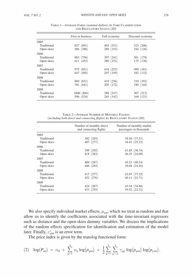
A simple comparison of average fares on international routes with and with-out open skies agreements suggests that open skies agreements have reduced fares for all fare classifications and that the reductions are sizable—by 2009 they were roughly 40 percent (Table 1). A similar comparison also shows that routes with open skies agreements have had more flights even though they had fewer passen-gers, with the difference peaking at close to 10 percent during 2007 and 2008 (Table 2). Of course, those comparisons do not hold any other influences on fares and flight frequency constant. We do so by specifying a plausible model of interna-tional airline markets.
II. Empirical Specification
Our simultaneous equations model of international airline markets specifies the demand and supply, including fares and flight frequency, for air transportation, the agreement (traditional or open skies) negotiated by the two countries that governs market competition, and the market structure, measured by the number of carriers on the route.
A. Demand
We measure fares and passenger demand by fare classification, discount economy, full economy, and business and first class, where the fare is the weighted (by number of passengers) average fare across all airline products in that fare classification and the number of passengers is obtained by aggregating the passengers choosing those products. Airline products are defined by carrier (e.g., United Airlines) and airport itinerary (e.g., nonstop between Washington, DC Dulles International Airport and London Heathrow Airport).
We use Hausman’s (1996) two-level approach, where the top level corresponds to the overall demand for air travel in the market, and the bottom level corresponds to the allocation of total demand among the three fare classifications (referred to as market segments), conditional on total expenditures. We model the bottom level

VOL. 7 NO. 2 377WINSTON AND YAN: OPEN SKIES
0
1
2
3
0 2,000 4,000 6,000 8,000 10,000Distance
Yield of business or first class in dollars per mile: 2009 Fractional polynomial fit
0
0.5
1
1.5
2
2.5
0 2,000 4,000 6,000 8,000 10,000Distance
Yield of economy full in dollars per mile: 2009 Fractional polynomial fit
Figure 2B. The Relationship between Yield and Distance for Full Economy in 2009
Notes: The plots for other years in the sample have a similar pattern. The means of the yields in nominal US dollars are: 0.34 in 2005, 0.34 in 2006, 0.36 in 2007, 0.37 in 2008, and 0.32 in 2009.
Figure 2A. The Relationship between Yield and Distance for First and Business Class in 2009
Notes: The plots for other years in the sample have a similar pattern. The means of the yields in nominal US dollars are: 0.58 in 2005, 0.60 in 2006, 0.64 in 2007, 0.67 in 2008, and 0.61 in 2009.

378 AMERICAN ECONOMIC JOURNAL: ECONOMIC POLICY MAY 2015
using the flexible Almost Ideal Demand System (Deaton and Muellbauer 1980), so demand for a market segment is given by:
(1) s gmt = α g + β g log ( E mt ___ P mt ) + ∑
g ′ =1
3
γ g g ′ log ( p g ′ mt ) + ϑ g log ( L m )
+ μ gr + μ gc + μ gy + μ gt + μ gm + ε gmt s , g = 1, 2, 3,
where s gmt is the revenue share of segment g in market m (e.g., Washington, DC, Dulles to London, Heathrow) in month t ; E mt is the overall market expenditure in month t and P mt is a price index; p g
′ mt is the full price (including taxes) of segment
g ′ ; and L m is the distance between the end-point airports. We include fixed effects dummy variables for regions of the world (Europe, North America, and so on), μ gr , the end-point countries, μ gc , year, μ gy , and month, μ gt . The regional dummy variables indicate routes where both the origin and destination airports are located within a given region so they capture the effects of free trade agreements (e.g., within the European Union and North America).
As an illustration of how we specify the regional and country dummies, for the Washington, DC–Mexico City route we specify one regional dummy variable (North America) and two country dummy variables (one for the United States and another for Mexico). There are a total of 90 countries in our sample. An alternative specification would include country-pair dummies, so the United States and Mexico would comprise such a dummy. There are a total of 242 country-pairs in our sample. As we explain later, our empirical findings are robust with respect to the alternative ways of controlling for country effects.
0
0.5
1
1.5
0 2,000 4,000 6,000 8,000 10,000Distance
Yield of discount economy in dollars per mile: 2009 Fractional polynomial fit
Figure 2C. The Relationship between Yield and Distance for Discount Economy in 2009
Notes: The plots for other years in the sample have a similar pattern. The means of the yields in nominal US dollars are: 0.24 in 2005, 0.22 in 2006, 0.23 in 2007, 0.24 in 2008, and 0.21 in 2009.
VOL. 7 NO. 2 379WINSTON AND YAN: OPEN SKIES
We also specify individual market effects, μ gm , which we treat as random and that allow us to identify the coefficients associated with the time-invariant regressors such as distance and the open-skies dummy variables. We discuss the implications of the random effects specification for identification and estimation of the model later. Finally, ε gmt s is an error term.
The price index is given by the translog functional form:
(2) log ( P mt ) = α 0 + ∑ g=1
3
α g log ( p gmt ) + 1 _ 2 ∑ g=1
3
∑ g ′ =1
3
γ g g ′ log ( p gmt ) log ( p g
′ mt ) .
Table 1—Average Fares (nominal dollars) by Fare Classification and Regulatory Status (SD)
First or business Full economy Discount economy
2005 Traditional 827 (691) 403 (251) 323 (206) Open skies 586 (388) 289 (153) 184 (126)2006 Traditional 883 (756) 397 (241) 301 (178) Open skies 611 (452) 289 (152) 175 (130)2007 Traditional 975 (851) 418 (253) 309 (181) Open skies 647 (505) 297 (159) 182 (132) 2008 Traditional 969 (831) 419 (256) 310 (192) Open skies 701 (641) 205 (172) 190 (144)2009 Traditional 1000 (884) 389 (247) 307 (213) Open skies 596 (524) 245 (142) 164 (123)
Table 2—Average Number of Monthly Flights (including both direct and connecting flights) by Regulatory Status (SD)
Number of monthly direct and connecting flights
Number of monthly market passengers in thousands
2005 Traditional 382 (293) 39.50 (37.51) Open skies 407 (277) 34.41 (25.23)2006 Traditional 399 (292) 41.85 (38.74) Open skies 418 (283) 36.35 (24.09)2007 Traditional 409 (287) 44.53 (40.24) Open skies 446 (283) 39.68 (24.56)2008 Traditional 417 (277) 43.93 (37.35) Open skies 452 (276) 40.11 (23.71)2009 Traditional 424 (267) 43.54 (34.86) Open skies 433 (255) 39.52 (22.31)

380 AMERICAN ECONOMIC JOURNAL: ECONOMIC POLICY MAY 2015
Assuming travelers maximize utility, we impose the following well-known restrictions on the demand parameters:
(3) Adding-up:
∑ g=1
3
α g = 1, ∑ g=1
3
β g = 0, ∑ g=1
3
γ g g ′ = 0 ∀ g ′ = 1, 2, 3, ∑
g=1
3
ϑ g = 0,
∑ g=1
3
μ gr = 0, ∑ g=1
3
μ gc = 0, ∑ g=1
3
μ gy = 0, and ∑ g=1
3
μ gt = 0 .
(4) Homogeneity: ∑ g ′ =1
3
γ g g ′ = 0, ∀ g = 1, 2, 3
(5) Symmetry: γ g g ′ = γ g ′ g .
The adding-up constraints in equation (3) imply that it is appropriate to use only two of the three revenue share equations in estimation to avoid the singularity problem. Because the choice of which two does not affect the estimation results, we drop segment 3, discount economy.
The volume of air travel in a nondirectional airport-pair market captures a portion of the origin and destination countries’ trade in the aviation service sector; thus, we specify the top level demand as a gravity equation, which is the most commonly used functional form to model trade flows:
(6) log ( Q mt ) = θ 0 + θ 1 log ( P mt ) + θ 2 log ( K mt ) + θ 3 log ( N mt ) + θ 4 log ( I mt )
+ θ 5 log ( L m ) + ϖ r + ϖ c + ϖ y + ϖ t + ϖ m + τ m T + ε mt Q ,
where Q mt is the number of air travelers in market m at time t ; P mt is the price index given in equation (2); K mt is the number of monthly direct and connecting flights; N mt is the geometric mean of the populations of the end-point countries at time t ; I mt is the geometric mean of the per capita incomes of the end-point countries at time t ; ϖ r , ϖ c , ϖ y , and ϖ t are fixed regional, end-point countries, year, and month effects; ϖ m denotes the random market effects that are allowed to be correlated with the regressors; and τ m T , where τ m is a random component with zero mean and T denotes the time trend, captures the random market trend.9 The number of flights affects market demand because more frequent flights reduce the costs of schedule delay, defined as the difference between travelers’ preferred departure times and their actual departure times, which increases the attractiveness of air compared with alternative modes and increases its market share and the size of the travel market.10
9 We explored functional specifications that included a linear and a squared term for distance for the top-level demand equation and for other equations in our model where distance appeared, but we did not obtain statistically significant estimates of the squared term.
10 The literature is much less clear on whether the number of flights, which does not vary by fare classification, affects the expenditure shares, all else constant, and on the signs of those effects. We explored the matter empirically

VOL. 7 NO. 2 381WINSTON AND YAN: OPEN SKIES
B. Supply
If airlines operate in an international market that is not subject to economic regulations, they decide on the number of flights to offer and the fares to charge for those flights to maximize profits. If carriers operate in a regulated market, they may or may not be able to determine their flight frequencies while fares are set by the regulatory agreement. Given the constraints imposed on airlines when they operate in a regulated market, we do not attempt to build a structural model of airline behavior; instead, we simply indicate that our empirical model resembles a two-stage game of airlines’ supply decisions, where airlines first determine their flight frequency and then set fares given frequency. We then measure the effect of an open skies agreement on competition in a market that may increase the num-ber of flights and reduce fares by reducing carriers’ costs or their price markups or both.
Drawing on the US airline deregulation experience, an open skies agreement will have an initial—and potentially large—effect on carriers’ pricing and operating behavior shortly after it is implemented and have effects that persist over time as carriers adjust to the change in the competitive environment. We therefore capture an open skies agreement’s cumulative effect on fares and flight frequency by speci-fying dummy variables to indicate its effects in the short and long run. Because our sample covers the 2005 to 2009 period, we capture the initial or short-run effects of the 12 open skies agreements (covering 35 of the 415 routes in the sample) that were signed after 2005 and the long-run effects of the 67 open skies agreements (covering 144 of the 415 routes) that were signed before 2000. Only 3 open skies agreements (covering 11 routes in the top 500 routes of the initial sample) were signed during 2000 to 2005, preventing us from capturing the intermediate effects of the agreements because they were collinear with the regional and end-point country dummies.
We do not directly model flight frequency because, as indicated by equation (6), it affects market demand and, subject to the regulatory agreement, it is adjusted by airlines to respond to changes in demand. Thus, it is very difficult to uniquely identify both demand and frequency, although we later specify instruments for fre-quency to estimate its effect on demand. Instead, we model the long-run equilib-rium relationship in a market between demand and flight frequency by drawing on Belobaba, Odoni, and Barnhart’s argument (2009, 159) that airlines choose flight frequency to achieve a target load factor as part of their long-run fleet planning process. The load factor, which is defined as the percentage of seats filled by paying passengers, is our measure of capacity utilization that we model as a function of market characteristics. We make the plausible assumption that aircraft size (number of seats) in most international markets can be taken as given because it is largely determined by market characteristics, such as the population at the endpoint cities, distance, and airport size. For a given aircraft size, the number of flights is therefore equivalent to the total number of seats.
and found that the number of flights was highly correlated with total expenditures and produced very imprecise parameter estimates and implausible elasticities.

382 AMERICAN ECONOMIC JOURNAL: ECONOMIC POLICY MAY 2015
Based on airlines’ long-run fleet planning process, we expect and later verify empirically with Augmented Dickey-Fuller tests that passengers and flights are cointegrated—that is, some linear combination of them is stationary—to maintain a long-run equilibrium relationship in capacity utilization. Formally, let (1, δ 1 ) denote the normalized cointegrating vector, where cointegration implies that long-run equi-librium capacity utilization is defined by log ( K mt ) + δ 1 log ( Q mt ) = e mt . In the spe-cial case that the cointegrating vector is (1, −1), then e mt is simply the log of flights to demand ratio, which measures the log of the (inverse) load factor. We expect the target (inverse) load factor in a market to depend on the population and per capita income of the cities that comprise the end-point airports because those variables determine market size, and also to depend on the market structure, regulatory status, the length of haul, and other market characteristics including the presence of an alliance. We therefore specify:
(7) e mt = δ 2 log ( N mt ) + δ 3 log ( I mt ) + δ 4 log ( C mt )
+ δ 5 A mt + δ 6 OS A m l + δ 7 OS A mt s + δ 8 log ( L m )
+ X mt K Γ K + ζ r + ζ c + ζ y + ζ q + ζ m + ε mt K ,
where population, income, and length of haul have been defined previously. We measure market structure with C mt , the number of carriers, and account for the pres-ence of a major airline alliance in market m at time t with a dummy variable A mt ; OS A m l is a dummy variable indicating the open skies status of market m in the long run (1 if an open skies agreement was signed before 2000; 0 otherwise); OS A mt s is a dummy variable indicating the open skies status of market m in the short run (1 if an open skies agreement was signed after 2005; 0 otherwise); X mt K is a vector of route-level attributes that affect airlines’ flight scheduling decisions, including the difference between the historical average monthly rainfall and temperature at the ori-gin and destination airports and the number of cities connected to the end-point air-ports. We also include regional, end-point countries, year, and monthly fixed effects ( ζ r , ζ c , ζ y and ζ t ) and random market effects ( ζ m ) , which are allowed to be correlated with the regressors. Those effects include, for example, variations in aircraft size and load factors. Finally, ε mt K represents the long-run equilibrium error in capacity utilization. Because the error has to be a stationary series, we test whether open skies agreements have caused long-run equilibrium capacity utilization to undergo a structural change.
We specify airlines’ pricing decisions by first noting that conditional on market passengers, flight frequency affects air fares through short-run fluctuations in capac-ity utilization that are captured by e mt . The remaining direct influences on fares, market structure, the presence of a major airline alliance, and the status of the open skies agreements affect markups, while carriers’ operating costs and thus fares are affected by trip distance interacted with the price of crude oil at time t, O t , and other

VOL. 7 NO. 2 383WINSTON AND YAN: OPEN SKIES
route-level characteristics, X mt f , including historical average monthly rainfall and temperature. Thus, we specify the fare equations as:
(8) log ( f gmt ) = ϕ 0g + ϕ 1g log ( Q mt ) + ϕ 2g ( e mt ) + ϕ 3g log ( C mt )
+ ϕ 4g A mt + ϕ 5g OS A m l + ϕ 6g OS A mt s + ϕ 7g log ( L m )
+ ϕ 8g log ( L m × O t ) + X mt f Γ g f + ξ rg + ξ cg
+ ξ yg + ξ tg + ξ mg + ε gmt f , g = 1, 2, 3 ,
where we also include regional, end-point countries, year, and monthly fixed effects ( ξ rg , ξ cg , ξ yg , and ξ tg ) and random market effects ( ξ mg ), which are allowed to be cor-related with regressors; and ε gmt f is an error term.
C. Market Structure
An open skies agreement also affects fares by affecting market structure, namely the number of carriers in an international airline market, because airlines are free to enter the market to provide service, while they are generally unable to do so in a reg-ulated environment. Our specification includes dummy variables indicating whether an open skies agreement was negotiated in the short run and the long run, fare reve-nues, which help determine potential profits, and exogenous market characteristics. We also include a random market time trend, ψ m T , where ψ m is a random component with zero mean and T is a time trend, because we expect the evolution of a market’s structure to be time-persistent and to be different in different markets—an expecta-tion confirmed by time series plots of the number of carriers in each market.
Our empirical model of market structure is therefore:
(9) log ( C mt ) = π 0 + π 1 OS A m l + π 2 OS A mt s + π 4 log ( R mt ) + π 5 A mt
+ π 6 log ( L m ) + X mt M Γ M + ϑ r + ϑ c
+ ϑ y + ϑ t + ϑ m + ψ m T + ε mt M ,
where R mt is total fare revenues in market m at time t and X mt M is a vector of market characteristics that are likely to affect post-entry variable profits and the fixed-costs of entry, including the number of cities connected to the airports that serve the end-point cities and the number of carriers in the end-point countries; the presence of a major airline alliance, A mt , may affect market structure by enabling an airline to use its partner’s network to serve a market; ϑ r , ϑ c , ϑ y , and ϑ t are regional, end-point countries, year, and monthly fixed effects, and ϑ m denotes random market effects correlated with the regressors; and ε mt M is an error term.
In sum, our modeling system consists of three demand and three fare equations, an equilibrium capacity utilization equation, and a market structure equation. We account for the common parameters that arise in the demand equations because

384 AMERICAN ECONOMIC JOURNAL: ECONOMIC POLICY MAY 2015
the price index specified in equation (2) appears in the three equations and for the symmetry condition in equation (5) that restricts the substitution pattern across seg-ments. The demand equations are also nonlinear in parameters because the price index is multiplied by β g in equation (1) and by θ 1 in equation (6).
III. Identification and Estimation
We use the logic of difference-in-differences (DID) methodology to identify the short-run effects of open skies agreements on market outcomes because a control group of markets exists whose regulatory status was unchanged; identification of the long-run effects relies on cross-sectional variation across markets. One possible concern with this identification strategy is that OSAs involving the United States tend to be with countries that are more developed than are other countries, which may lead to an upward bias in the effects of OSAs. However, we hold constant the difference between the control group of markets and the treatment group of markets by including individual end-point country dummy variables and observed country characteristics, such as population and income, in the specification. In addition, the full sample includes OSAs between countries that are not among the most devel-oped English speaking countries. As we report later, the effect of OSAs on travelers’ fares is actually somewhat larger for the full sample than for the subsample of US international routes in which the only OSAs involve the United States, which also casts doubt that the estimates of the US OSAs are upward biased.
Because open skies agreements are negotiated at the country-pair level instead of at the route level, we included dummy variables for the end-point countries in the specification of all of the equations to control for omitted group effects at the country level. The estimates obtained from specifying end-point country dummy variables are equivalent to those obtained by specifying country-pair dummy vari-ables when we restrict the sample to include only US international routes, which is the basis for our policy simulations. However, when we perform estimations using the full sample, it is possible that the end-point country dummy variables may not control fully for the effect of free trade agreements between two countries on fares, market structure, and capacity utilization, and that it would be preferable to specify country-pair dummy variables to control for that effect. So, we checked the robust-ness of our findings by replacing the end-point country dummy variables with the country-pair dummy variables in our model and we found that the estimated effects of the OSAs hardly changed. This may be because the regional dummy variables that we include, such as for the European Union and North America, also capture the effect of free trade agreements.
The random effects regression equations in our model can be expressed in general form as:
(10) y mt = X mt B 1 + W m B 2 + c m + ψ m T + ε mt ,
where y mt is a dependent variable in market m at time t that we seek to explain; c m represents the individual market effects that we model as random; ψ m T is the random

VOL. 7 NO. 2 385WINSTON AND YAN: OPEN SKIES
market trend specified in the top-level demand and market structure equations; ε mt is the idiosyncratic random shocks; X mt is a vector of time-varying regressors that are allowed to be correlated with random components; and W m is a vector of exogenous time-invariant regressors that include route distance, regional, end-point country, year, and month dummies in most equations. This random effects specification is similar to Hausman and Taylor (1981).
Challenges to identification arise in our model because we allow the random mar-ket effects to be correlated with regressors and because the endogenous variables, passenger demand, fares, flight frequency, market structure, and regulatory status, are also specified as explanatory variables. When a regressor in X mt is correlated with the three random components ( c m , ψ m T , and ε mt ), we use the demeaned first-order difference of z mt as its instrument, where z mt is a variable uncorrelated with ε mt and the process of demeaning and first-order differencing removes its correlation with the random market effects and the random market trend. When a regressor in X mt is correlated with c m and/or ψ m T but not with ε mt , demeaning and/or first-order differ-encing this variable leads to a valid instrument.
In some cases, certain variables can serve as instruments ( z mt ) because we hold other variables in the specification constant. For example, the demeaned income and population of the origin and destination countries are valid instruments for market expenditures in the bottom-level demand equation because relative segment prices and expenditures are held constant. Potential simultaneity bias is therefore avoided because fare class choice is not affected by changes in income and population. As another example, the demeaned total bilateral trade value is a valid instrument for the short-run regulatory status dummy variable in the capacity utilization equa-tion (7) and in the fare equation (8) because the number of market passengers is held constant. We summarize the estimable equations, the endogenous variables in those equations, and their instruments in Table 3, and discuss our identification strategies in detail in the Appendix.
We explored first-stage regressions for each equation by regressing the endoge-nous variables on the instruments and we found that all coefficients were statistically significant, indicating that the instruments are correlated with the endogenous vari-ables. The main results of those regressions are presented in Appendix Tables A1–A3. Later we present robustness tests of our estimated models based on alternative approaches to constructing the instruments.
Turning to estimation, let Z mt denote a vector of instruments including both exog-enous regressors and instruments for the endogenous regressors; thus, the regres-sion equations in our model are identified by the mean independence condition E ( c m + ψ m T + ε mt | Z mt ) = 0 . We estimate the parameters of the model by Gen-eralized Method of Moments (GMM), which employs the orthogonal conditions implied by the mean independence condition as moment functions, and accounts for the correlations within an equation that arise from our random market effects specification. Accordingly, identification and estimation of the model do not rely on any distributional assumptions for the error terms.
We could further improve estimation efficiency by accounting for the contempo-raneous correlation of the errors across equations but we found that it was not com-putationally feasible to simultaneously estimate the large number of parameters that

386 AMERICAN ECONOMIC JOURNAL: ECONOMIC POLICY MAY 2015
Table 3—Equations, Endogenous Variables, and Instruments
Equations Endogenous variables Source of endogeneity Instruments
Expenditure share equations (equation (1) in the text)
Segment prices ( p gmt ) and price index ( P mt )
Correlation with random market effects and simultaneity bias
Demeaned segment average taxes
Market expenditure ( E mt ) Correlation with random market effects and simultaneity bias
Demeaned market population and income per capita, which affect market expenditure by affecting market demand
Market demand equation (equation (6) in the text)
Segment prices ( p gmt ) and price index ( P mt )
Correlation with random market effects and simultaneity bias
Same as those in the share equations
Market population and per capita income ( N mt , I mt )
Correlation with random market effects
Demeaned market population and per capita income
Number of flights ( K mt ) Correlation with both random market effects and random market trends; simultaneity bias
Demeaned first-order difference of last year’s log number of flights
Equilibrium capacity utilization equation (equation (7) in the text)
Presence of alliance ( A mt ) Correlation with random market effects
Demeaned alliance presence
Regulatory status (OS A mt s ) Correlation with random market effects and simultaneity bias
Demeaned imports and exports between the two countries
Market population and per capita income ( N mt , I mt )
Correlation with random market effects
Demeaned market population and per capita income
Number of carriers ( C mt ) Correlation with both random market effects
Demeaned number of carriers
Segment fare equations (equation (8) in the text)
Regulatory status (OS A mt s ) Correlation with random market effects and simultaneity bias
Demeaned imports and exports between the two countries
Number of passengers ( Q mt ) Correlation with random market effects and simultaneity bias
Demeaned market population and income-per capita, which affect market demand
Number of carriers ( C mt ) and presence of alliance ( A mt )
Correlation with random market effects
Demeaned number of carriers and alliance presence
Short-run fluctuation in equilibrium capacity utilization ( e mt )
Correlation with random market effects
Demeaned equilibrium capacity utilization
Market structure equation (equation (9) in the text)
Regulatory status (OS A mt s ) Correlation with random market effects and with random market trend
Demeaned first-order difference of regulatory status
Market fare revenue ( R mt ) Simultaneity bias and correlation with both random market effects and random market trend
The price of crude oil
Presence of an airline alliance ( A mt )
Correlation with random market effects
Demeaned first-order difference of the presence of an alliance

VOL. 7 NO. 2 387WINSTON AND YAN: OPEN SKIES
resulted from specifying eight equations that each included regional, end-point coun-try, year, and monthly dummy variables.11 We therefore estimate the three demand equations jointly to account for their common parameters and cross-equation con-straints given in equations (3)–(5), and then estimate the remaining equations indi-vidually. It turns out that the main parameters of interest are estimated precisely and that the additional gain from estimating the eight equations jointly is likely to be small. We provide a formal presentation of the estimation procedure in the Appendix.
IV. Estimation Results
The United States has negotiated many open skies agreements with other countries and could negotiate even more in the future; thus, our main objective is to estimate travelers’ benefits from open skies agreements on US international routes. We do so by first estimating our model using a subsample that contains only US interna-tional routes because it is appropriate to use parameter estimates obtained from that subsample to perform the welfare calculations. As noted, we do not extrapolate our findings to all US international routes and raise the possibility of selectivity bias. However, given the full sample is more representative of international airline mar-kets, it is important to also estimate our model using the full sample to check the robustness of the parameter estimates obtained from the subsample.
GMM parameter estimates of the demand, capacity utilization, fare, and market structure equations for both samples are easier to digest if we report them in separate tables. Tables 4 and 5 present the top and bottom level (expenditure share) demand
11 Joint estimation is further complicated because the market demand and market structure equations use lagged variables as instruments and are therefore estimated using subsamples of the full dataset.
Table 4—GMM Top-Level Demand Estimates (SE )
Dependent variable: log number of
market passengers
Dependent variable: log number of
market passengers
Full sample
US international routes only
log price index −0.3064 (0.1247) −0.4680 (0.1843)log number of flights 0.2625 (0.1311) 0.1845 (0.0982)log distance 0.0910 (0.0588) 0.1756 (0.0724)log geometric mean population of the end-point countries 2.1275 (0.7478) 4.0369 (1.9514)log geometric mean of income per capita of the end-point countries 0.3701 (0.1433) 1.2048 (0.2995)Regional dummies included Yes YesCountry dummies included Yes YesYear dummies included Yes YesMonthly dummies included Yes YesRandom market effects taken into account Yes YesNumber of markets (directional routes)a 408 66
Observations 17,572 2,940
a As noted in footnote 11, market demand is estimated using lagged variables as instruments, which slightly reduces the number of markets in the final estimation using the full sample.

388 AMERICAN ECONOMIC JOURNAL: ECONOMIC POLICY MAY 2015
equations. The overall price elasticities of air travel demand, conditional on a fixed number of flights, are −0.31 for the full sample of international routes and −0.47 for the subsample of US international routes. We compare the unconditional demand elasticities, reported later, with those in the literature. Generally, the other param-eter estimates in the two samples are of similar magnitude and have the expected sign: a greater number of flights increases demand with an elasticity between 0.26 and 0.18; distance has a positive effect on demand, reflecting air’s speed advantage over other modes, which reduces travel time costs for longer distance trips;12 and demand is stimulated by an increase in the mean population and income per capita of the end-point countries. The population and income elasticities on US interna-tional routes are greater than those on the full sample of routes, in all likelihood because compared with populations in many other countries, a smaller share of the US population travels abroad so a change in population will yield a larger demand elasticity and because compared with the United States, other countries have a much
12 Distance’s coefficient is for the average distance in our sample. The effect of distance on demand is likely to weaken for longer distances because alternative modes to air transportation are not viable.
Table 5—GMM Bottom-Level Demand (expenditure shares) Estimates (SE )
Revenue share of segment 1 (business or
first-class; g = 1 )(1)
Revenue share of segment 2 (economy
full; g = 2 )(2)
Revenue share of segment 3 (economy
discount or other; g = 3 )(3)a
Panel A. Full sample Constant 0.2236 (0.0007) 0.1511 (0.0009) 0.6253 (0.0015)log distance 0.0521 (0.0051) −0.1094 (0.0103) 0.0573 (0.0113)log real expenditure 0.0697 (0.0263) −0.3417 (0.0528) 0.2720 (0.0548)Interaction of log segment prices segment g and segment 1: γ g1 −0.0698 (0.0161) 0.0438 (0.0148) 0.0260 (0.0142) segment g with segment 2: γ g2 0.0438 (0.0148) −0.0650 (0.0186) 0.0212 (0.0108) segment g with segment 3: γ g3 0.0260 (0.0142) 0.0212 (0.0108) −0.0472 (0.0226)Number of markets (routes) 415 415 415
Observations 22,638 22,638 22,638
Panel B. US international routes onlyConstant 0.3308 (0.0028) 0.1070 (0.0026) 0.5622 (0.0024)log distance 0.0387 (0.0075) −0.0369 (0.0057) −0.0018 (0.0095)log real expenditure −0.0612 (0.0596) 0.0886 (0.0390) −0.0274 (0.0743)Interaction of log segment prices segment g with segment 1: γ g1 −0.0352 (0.0157) 0.0221 (0.0083) 0.0131 (0.0178) segment g with segment 2: γ g2 0.0221 (0.0083) −0.0751 (0.0164) 0.0530 (0.0167) segment g with segment 3: γ g3 0.0131 (0.0178) 0.0530 (0.0167) −0.0661 (0.0304)Number of markets (routes) 66 66 66
Observations 3,766 3,766 3,766
Regional dummies included Yes Yes —Country dummies included Yes Yes —Year dummies included Yes Yes —Monthly dummies included Yes Yes —Random market effects taken into account
Yes Yes —
a Parameter values of this equation are obtained from the parametric restrictions in equations (3), (4), and (5). The standard errors are calculated by using the bootstrap technique.

VOL. 7 NO. 2 389WINSTON AND YAN: OPEN SKIES
lower per capita income so many residents still cannot afford air travel even if their income rises.
Most of the parameter estimates in the expenditure share equations shown in Table 5 are precisely estimated. Their magnitudes and the differences between the samples are clearer when we use them below to calculate the own and cross-price elasticities of segment demand.
The cointegrating vector between market passengers and the number of flights enabled us to construct the short-run fluctuations in equilibrium capacity utilization, which we included in the airline fare equations. We can estimate the cointegrating vector and other parameters in the equilibrium capacity utilization equation (7) by regressing log ( K mt ) on log ( Q mt ) and the other explanatory variables. The estimation results presented in Table 6 include specifications in the first and third columns with passenger demand as the only regressor and specifications in the second and fourth
Table 6—GMM Estimates of Equilibrium Capacity Utilization (SE )
Full sample
(1)
Full sample
(2)
US international routes only
(3)
US international routes only
(4)
log number of market passengers in a month 0.6588(0.0048)
0.6174(0.0088)
0.7347(0.0274)
0.6825(0.0203)
Short-run open skies dummy (1 if an OS agreement was signed after 2005; 0 otherwise)
0.1181(0.0591)
0.1605(0.0534)
Long-run open skies dummy (1 if an OS agreement was signed before 2000; 0 otherwise)
−0.0455(0.0748)
−0.0026(0.3441)
log geometric mean population of the end-point countries
0.3460(0.2381)
2.2522(1.2726)
log geometric mean of income per capita of the end-point countries
0.3205(0.0473)
0.2598(0.1734)
log number of carriers 0.0282(0.0109)
0.0999(0.0337)
Presence of an airline alliance −0.0158(0.0120)
0.0324(0.0523)
log distance −0.2020(0.0096)
−0.4946(0.0175)
log number of cities connected to the end-point airports
0.4866(0.0327)
0.8522(0.0408)
Maximal historical average rainfall at the end-point cities in a montha
−0.0432(0.0324)
−0.3864(0.0915)
Maximal temperature difference between January and July at the end-point citiesb
−0.0061(0.0008)
−0.0135(0.0012)
Regional dummies included No Yes No YesCountry dummies included No Yes No YesYear dummies included No Yes No YesMonth dummies included No Yes No YesRandom market effects taken into account Yes Yes Yes YesNumber of markets (nondirectional routes) 415 415 66 66
Observations 22,638 22,638 3,766 3,766
a This variable is measured as the maximal value of the historical average monthly rainfall (000’s mm) at the two end-point cities. Data were obtained from airport websites.
b This variable is measured as the maximal value of the difference in the average temperature between July and January at the two end-point cities. Data were obtained from airport websites.

390 AMERICAN ECONOMIC JOURNAL: ECONOMIC POLICY MAY 2015
columns that also include the other regressors. The estimated signs of the regressors are plausible as population, income, number of carriers, and the number of cities connected to the endpoint airports have a positive effect on the number of flights, while distance, rainfall, and temperature differences at the endpoint airports have a negative effect. The negative effect of distance indicates that as routes become longer, airlines find it more efficient to operate larger planes with lower frequency than to operate smaller planes with greater frequency. In both samples, open skies agreements increase the number of flights in the short run and have a statistically insignificant effect in the long run, while the presence of an alliance has a statisti-cally insignificant effect.
We use the parameter estimates from the full sample (column 2) to predict the residuals so that we can test whether passengers and flights are in fact cointegrated (the value of the cointegrating vector was robust to the alternative specifications). We define:
(11) e ̂ mt = log ( K mt ) − 0.6174 × log ( Q mt ) ,
and implement the Augmented Dickey-Fuller (ADF) test of cointegration by esti-mating the following fixed-effects model:
(12) Δ e ̂ mt = ρ e ˆ m (t−1) + ∑ j=1
p
ρ ˜ j Δ e ̂ m (t−j) + X ˜ mt B + b m e + ε mt e ,
where X ˜ mt is a vector of regressors including market characteristics such as popu-lation, per capita income, number of carriers, and year and month dummies. Under the null hypothesis that the log number of flights and the log number of market passengers are not cointegrated, the parameter ρ = 0 ; ρ < 0 under the alternative hypothesis that those two series are conintegrated. We report OLS estimates of ρ based on alternative specifications in the Appendix Table A4 for the full sample and also for the sample of US international routes (using the parameter estimates from column 4, Table 6). All of the coefficient estimates are less than zero and have large t-statistics, providing strong empirical support for the hypothesis that market pas-sengers and the number of flights are cointegrated in both samples.
The responsiveness of segment demands, market demand, and the number of flights with respect to a change in segment prices, overall price, and monthly flights can be calculated only numerically; we describe our approach in the Appendix. As shown in Table 7, the own-price elasticities for both samples have the correct negative sign and their magnitudes imply that travelers in the full sample who fly first class, business, and full economy are more responsive to fare changes in their segments than are travelers who fly discount economy, in all likelihood because air fares constitute a larger share of the total cost of their trips and because fewer people fly in those segments so a given change in price will produce a larger elas-ticity. Those factors may also explain why travelers on US international routes who fly full economy have the greatest response to fare changes in their segment. The unconditional price elasticities of market demand are, as expected, larger than the conditional elasticities obtained previously from the top-level demand model

VOL. 7 NO. 2 391WINSTON AND YAN: OPEN SKIES
because they account for the change in the number of flights. Their magnitudes, −0.39 for the full sample of international routes and −0.53 for the subsample of US international routes, are bounded by the mean price elasticity for business travelers, −0.27, and the mean price elasticity for pleasure travelers, −1.04, that are reported in an extensive survey of air travel demand elasticities by Gillen, Morrison, and Stewart (2003).
Generally, the cross-price elasticities indicate, as expected, that an increase in the fares of one segment increase the demand in the other segments and decrease total demand and monthly flights. An increase in the overall price reduces segment demands and flights. And increases in monthly flights increase segment demands and total demand.
The effects of the open skies dummies on fares are of particular importance to our analysis. As shown in Table 8, the initial (short-run) effect of an open skies agree-ment is to reduce fares approximately 50 percent or more in the full sample and approximately 25 percent or more in the subsample of US international routes; its additional long-run effect is to reduce fares approximately 15 to nearly 30 percent
Table 7—Estimated Demand and Flight Elasticities [5th percentile, 95th percentile]
Percent change in demand of
business or first class
Percent change in demand of economy full
Percent change in demand of
economy discount
Percent change in total market
demand
Percent change in number of
monthly flights
Panel A. Full sample a
One percent increase in the price of business or first class
−1.36[−1.52, −1.22]
0.63[0.51, 0.77]
0.01[−0.06, 0.04]
−0.06[−0.10, −0.02]
−0.04[−0.06, −0.01]
One percent increase in the price of economy full
0.26[0.17, 0.34]
−1.14[−1.37, −0.91]
0.09[0.02, 0.17]
−0.07[−0.10, −0.03]
−0.04[−0.06, −0.02]
One percent increase in the price of economy discount
0.63[0.40, 0.89]
0.91[0.63, 1.24]
−0.56[−0.80, −0.35]
−0.24[−0.40, −0.08]
−0.15[−0.25, −0.05]
Overall price (one percent increase in the prices of all segments)
−0.48[−0.78, −0.18]
0.05[−0.16, 0.21]
−0.52[−0.81, −0.21]
−0.39[−0.58, −0.15]
−0.23[−0.36, −0.09]
One percent increase in the number of monthly flights
0.34[0.04, 0.60]
−0.03[−0.34, 0.27]
0.37[0.04, 0.63]
0.28[0.03, 0.46]
—
Panel B. US international routes only a
One percent increase in the price of business or first class
−1.08[−1.28, −0.89]
0.13[−0.28, 0.58]
−0.03[−0.18, 0.09]
−0.14[−0.24, −0.05]
−0.10[−0.16, −0.03]
One percent increase in the price of economy full
0.13[−0.02, 0.26]
−1.73[−1.89, −1.56]
0.17[0.07, 0.25]
−0.06[−0.11, −0.01]
−0.04[−0.08, −0.01]
One percent increase in the price of economy discount
0.61[0.35, 0.88]
1.20[0.72, 1.72]
−0.70[−0.96, −0.43]
−0.32[−0.54, −0.10]
−0.21[−0.37, −0.07]
Overall price (one percent increase in the prices of all segments)
−0.38[−0.76, −0.14]
−0.47[−0.93, −0.17]
−0.57[−1.02, −0.26]
−0.53[−0.97, −0.24]
−0.36[−0.67, −0.17]
One percent increase in the number of monthly flights
0.12[0.01, 0.28]
0.17[0.01, 0.37]
0.20[0.01, 0.42]
0.18[0.01, 0.36]
—
a The elasticities are evaluated at the sample mean of the explanatory variables using Algorithm 1 in Appendix C. We calibrate the intercepts of the demand equations and the capacity utilization equation so that when those equa-tions are evaluated at the sample means of the explanatory variables, our model replicates the sample means of the market outcomes, which we use as the benchmark for the elasticity calculations. The sample means for the full sample are: market passengers 41,755; monthly flights 456; segment expenditure shares 0.22 (business plus), 0.15 (economy full), and 0.63 (economy discount); and segment prices (fare + tax) $870 (business plus), $406 (economy full), and $299 (economy discount). The sample means for US international routes only are: market passengers 38,000; monthly flights 409; segment expenditure shares 0.33 (business plus), 0.11 (economy full), and 0.56 (economy discount); and segment prices (fare + tax) $1537 (business plus), $506 (economy full), and $407 (economy discount). We use bootstrap techniques to construct the 95 percent confidence interval.

392 AMERICAN ECONOMIC JOURNAL: ECONOMIC POLICY MAY 2015
in the full sample and 20 percent or more in the subsample of US international routes.13 Note those estimates hold the number of carriers constant when, in fact, open skies agreements may enable more carriers to enter and compete on a route, which according to the parameter estimates in the table would further decrease fares in each segment, although the effects on full economy fares in both samples are not statistically significant.
We indicated in the introduction that it is important to distinguish between the effects on fares of open skies agreements and an airline alliance between two
13 We use the term approximately because the exact effect of a dummy variable in a log linear equation is given by 1 − exp(−COEFF), where COEFF is the coefficient of the dummy variable.
Table 8—GMM Estimates of the Fare Equations (SE )a
log fare of segment 1 (business plus)
(1)
log fare of segment 2 (economy full)
(2)
log fare of segment 3 (economy discount
or other)(3)
Panel A. Full sample Short-run open skies dummy −0.5726 (0.1286) −0.7019 (0.0830) −0.4996 (0.0796)Long-run open skies dummy −0.2041 (0.0264) −0.2836 (0.0195) −0.1492 (0.0171)log number of market passengers in a month 0.7224 (0.1032) 0.1832 (0.0940) 0.2276 (0.0728)Capacity utilizationb −0.0198 (0.0186) −0.0582 (0.0140) −0.0229 (0.0107)log number of carriers −0.1724 (0.0309) −0.0185 (0.0267) −0.0217 (0.0204)log distance 0.6431 (0.0295) 0.3210 (0.0263) 0.3812 (0.0200)log distance × crude oil price 0.0196 (0.0164) 0.0573 (0.0142) 0.0609 (0.0106)Presence of an airline alliance −0.0248 (0.0198) −0.0064 (0.0140) −0.0124 (0.0103)Maximal historical average monthly rainfall between the end-point citiesc
0.2722 (0.0540) 0.0682 (0.0427) 0.0258 (0.0343)
Maximal temperature difference between January and July at the end-point citiesd
0.0172 (0.0011) 0.0121 (0.0083) 0.0108 (0.0007)
Number of markets (routes) 415 415 415
Observations 22,638 22,638 22,638
Panel B. US international routes onlyShort-run open skies dummy −0.4886 (0.0456) −0.2621 (0.0375) −0.2476 (0.0436)Long-run open skies dummy −0.2509 (0.0480) −0.2058 (0.0412) −0.2412 (0.0448)log number of market passengers in a month 0.2945 (0.1043) 0.3121 (0.1009) 0.5715 (0.1278)Capacity utilizationb −0.0163 (0.0210) −0.0046 (0.0188) 0.0157 (0.0273)log number of carriers −0.0798 (0.0412) −0.0411 (0.0392) −0.1378 (0.0515)log distance 0.2943 (0.0309) 0.0820 (0.0315) 0.1609 (0.0424)log distance × crude oil price 0.0961 (0.0226) 0.0928 (0.0229) 0.0783 (0.0301)Presence of an airline alliance −0.2050 (0.0514) −0.1059 (0.0538) −0.2641 (0.0770)Maximal historical average monthly rainfall between the end-point citiesc
0.1712 (0.1200) 0.2102 (0.1223) 0.3202 (0.1512)
Maximal temperature difference between January and July at the end-point citiesd
0.0224 (0.0016) 0.0176 (0.0014) 0.0146 (0.0019)
Number of markets (routes) 66 66 66
Observations 3,766 3,766 3,766
a Region, country, year, and month fixed effects are included in all the regressions.b Capacity utilization is constructed by log ( K mt ) − 0.6174 log ( Q mt ) in the full sample and log ( K mt ) −
0.6825 log ( Q mt ) in the US subsample.c This variable is measured as the maximal value of the historical average monthly rainfall (000’s mm) at the two
end-point cities. Data were obtained from airport websites.d This variable is measured as the maximal value of the difference in the average temperature between July and
January at the two end-point cities. Data were obtained from airport websites.
VOL. 7 NO. 2 393WINSTON AND YAN: OPEN SKIES
international carriers. Our specification controls for the effect of an alliance (with antitrust immunity) on fares; thus, our finding that open skies agreements reduce fares cannot be partly attributed to the presence of alliances. Consistent with pre-vious research, we also find that an airline alliance (with antitrust immunity) on a route generally lowers fares. The coefficients, indicating fare reductions of 10 per-cent to 25 percent, are much larger and more precisely estimated for the subsample of US international routes than for the full sample, which may reflect the relative effectiveness of alliances that involve a US carrier. We have also noted that we do not account for traffic beyond the origin and destination airports, which may account for the small effects of alliances on fares in the full sample. In sum, although open skies agreements reduce travelers’ fares more than airline alliances do, the policies are related because the granting of antitrust immunity to a US carrier and its foreign alliance partner is approved by the US Department of Transportation only if an open skies agreement exists between the United States and the foreign partner’s country.
The remaining parameter estimates have the expected sign: fares are increased by greater passenger demand, given aircraft and airport capacity constraints, longer dis-tances, higher oil prices, greater rainfall that causes delays and increases operating costs, and larger temperature differences between January and July at the end-point airports that indicate higher operating costs during winter. Fares are reduced by an increase in capacity utilization, although the effect is not precisely estimated in the subsample of US international routes, possibly because load factors do not vary greatly over time and across those routes.
Finally, the market structure equation (Table 9) indicates that carriers in both samples adjust their networks after the countries at the origin and destination nego-tiate an open skies agreement. In the short run, the number of carriers on a route falls because inefficient carriers are no longer protected by price and entry regulations and they are driven out by more efficient carriers. In the long run, other carriers covered by the agreement have sufficient time to adjust their networks and take advantage of the opportunities to enter new international markets thereby increasing the number of carriers on a route. Thus, open skies agreements in the full sample and the subsample of US international routes have the direct effect of stimulating competition that reduces fares in the short run and continues to reduce them in the long run, and that increases flight frequency in the short run. And they have the indi-rect effect of increasing fares and decreasing flights in the short run by reducing the number of carriers on a route but decreasing fares and increasing flights in the long run by increasing the number of carriers on a route.
We again distinguish between the effects of open skies agreements and alliances in the specification and find that the number of carriers on a route increases when an alliance is formed. The remaining estimates indicate that total revenues, distance, and the number of carriers from the end-point countries are positively related to the number of carriers on a route, while an increase in the number of cities connected to the end-point airports reduces the number of carriers on a route, which may suggest a mega-carrier(s) is dominating the market.
In sum, we have analyzed a broad sample of international airline routes throughout the world and a subsample of US international airline routes, the former transporting more annual passengers, on average, and the latter generating more annual revenues,

394 AMERICAN ECONOMIC JOURNAL: ECONOMIC POLICY MAY 2015
on average, and we have found that travelers have benefited from open skies through lower fares and greater flight frequency in both samples. Using samples of routes with different levels of passenger demand and fares provides an important robustness check on our findings and suggests that air travelers on routes that are not included in our analysis may also benefit from open skies. As discussed in the Appendix and reported in Appendix Tables A5–A6, we also provide robustness checks by elimi-nating certain instruments whose exogeneity may be questioned because it is based on holding other variables in the specification constant and by exploring how our estimates of the open skies dummy variables are affected. The alternative estimates continue to indicate that travelers have benefited from open skies agreements. We now quantify the magnitude of those benefits.
V. Travelers’ Gains from Open Skies Agreements
How much have travelers gained from the open skies agreements that have been negotiated to date, and what additional gains could they realize if more countries negotiated agreements? We use the parameter estimates obtained from the subsam-ple of US international routes to address those questions because we can obtain more accurate estimates, especially given that the estimates of the short-run and long-run open skies dummy variables in the fare equations were economically and statistically significantly different from those estimated using the full sample. At the same time, because most of the parameter estimates in the subsample were broadly
Table 9—GMM Estimates of the Market Structure Equation (SE )
log number of carriersFull sample
log number of carriersUS international routes
only
Short-run open skies dummy (1 if an OS agreement was signed after 2005; 0 otherwise)
−0.2222(0.1205)
−0.1484(0.0891)
Long-run open skies dummy (1 if an OS agreement was signed before 2000; 0 otherwise)
0.1684(0.0270)
0.2279(0.0803)
log total fare revenue in a month 0.5336(0.0783)
0.2171(0.0582)
Presence of an airline alliance 0.1620(0.0209)
0.2765(0.0679)
log distance 0.1139(0.0204)
0.2098(0.0227)
log total number of carriers in the end-point countries 0.5501(0.0416)
0.3998(0.0785)
log number of cities connected to the end-point airports −0.2638(0.0431)
−0.1077(0.0542)
Regional dummies included Yes YesCountry dummies included Yes YesYear dummies included Yes YesMonth dummies included Yes YesRandom market effects taken into account Yes YesNumber of markets (routes) 415 66
Observations 22,275 3,709

VOL. 7 NO. 2 395WINSTON AND YAN: OPEN SKIES
similar in sign, statistical precision, and magnitude to those obtained from the full sample, they are sufficiently robust to use for welfare calculations.
Recall that the total gains from open skies agreements consist of initial short-run gains, which because our dataset covers travel during 2005 to 2009 we can measure for agreements negotiated after 2005, and additional long-run gains, which we can measure for agreements negotiated before 2000. We can therefore measure the ini-tial gains or additional long-run gains from an open skies agreement but not both. Specifically, we use our model to calculate the (short-run) change in consumers’ welfare on US international routes where airlines have been operating under open skies agreements that were signed between 2005 and 2009 (Appendix Table A7 shows there are 26 such routes in our sample) assuming those agreements did not exist. We then calculate the (additional long-run) change in consumers’ welfare on US international routes where airlines have been operating under open skies agree-ments that were signed before the year 2000 (Appendix Table A8 shows that there are 11 such routes in our sample) assuming those agreements did not exist. Finally, we show the potential gains to travelers from the United States negotiating open skies agreements with countries with which they have yet to do so by calculating the change in consumers’ welfare on US international routes where airlines have not been operating under open skies agreements as of 2009 (Appendix Table A9 shows there are 29 such routes in our sample) assuming those agreements did exist. In this case, we are able to calculate the initial and additional long-run gains from open skies agreements.
We determine the equilibrium number of carriers, flights, segment prices, and passengers for each counterfactual scenario by iterating the demand, capacity utili-zation, fare, and market structure equations after we assume a change in regulatory policy. We describe our algorithm in the Appendix. Calculations are performed for each month between 2005 and 2009 on each route.
We account for changes in both prices and service quality attributable to open skies agreements by first specifying a representative consumer’s expenditure func-tion corresponding to the Almost Ideal Demand System as (to simplify the exposi-tion, we drop the market and time subscripts)
(13) ln E ( u 0 , P) = log (P) + u 0 ∏ g=1
3
p g β g ,
where log (P) is defined in equation (2) and u 0 is the traveler’s initial (observed) indirect utility. If p e denotes the segment prices for a given counterfactual scenario obtained for a simulated equilibrium, e, then we can measure the compensating variation for the price effects alone by
(14) C V p = E ( u 0 , p e ) − E ( u 0 , p 0 ) .
We can then measure the compensating variation for the change in service quality—that is, the number of flights—by simulating the virtual segment prices (denoted by p V ) that yield the same equilibrium quantity of passengers as in the counterfactual scenario assuming we hold the number of flights at its initial level—that is, before

396 AMERICAN ECONOMIC JOURNAL: ECONOMIC POLICY MAY 2015
the change in regulatory policy. Thus, the additional change in welfare caused by the change in the number of flights K is given by
(15) C V K = E ( u 0 , p V ) − E ( u 0 , p e ) .
We can then compute the annual changes in travelers’ welfare by aggregating the compensating variations, C V p and C V K , per market and per month for each year from 2005 to 2009 and averaging the values over the five years. In sum, by compar-ing market outcomes under the counterfactual scenarios with observed outcomes during the sample period, we can quantify the initial and/or long-run effects of open skies agreements on the selected markets.14
As shown in Table 10, eliminating the open skies agreements on US international routes that have been signed between 2005 and 2009 would initially raise fares in all segments, with the greatest effect, 50 percent, on business and first-class fares; reduce passenger demand in all segments and market demand; reduce the number of flights; and increase the number of carriers per route.15 Travelers would lose $3 billion annually, nearly $2 billion from higher fares and $1 billion from fewer flights, indicat-ing that they gained substantially from the open skies agreements that had been nego-tiated during that period. As noted, we are understating the total gains because we cannot measure the additional long-run effects that would increase the initial gains.
We show in Table 11 that eliminating open skies agreements on US international routes that have been signed before 2000 would in the long run raise fares in all seg-ments, with the greatest effect, 26 percent, on business and first class fares; reduce pas-senger demand in all segments and market demand; reduce the number of flights, and reduce the number of carriers per route. Travelers would lose $0.84 billion annually, $0.7 billion from higher fares and $0.14 billion from fewer flights; total losses would, of course, be much greater. Thus, travelers’ gains from the open skies agreements that have been negotiated as of 2009 approach $4 billion annually, which is broadly consistent with the gains estimated by Cristea, Hummels, and Roberson (2012).16
14 As a conceptual point, our model provides estimates of the effect of signing an OSA but not of eliminating an OSA, while in our counterfactuals we explore how travelers’ welfare would change if OSAs were eliminated and if they were enacted. When we explore how travelers’ welfare would change if OSAs were eliminated on those routes that had them, we assume that the estimated effect of an OSA is zero and that the other coefficients are held constant. Those are reasonable assumptions even if no OSAs have actually been eliminated because many routes do not have OSAs, which means the OSA dummy takes on a value of zero, and the other coefficients should not change for a given value of the OSA dummy. When we explore how travelers’ welfare would change if OSAs were enacted, we assume the estimated effect of an OSA takes on the value that an OSA has had on other routes when it is in effect and that the other coefficients are held constant. We cannot assess that assumption, but it is the most plausible one we can make given the available evidence and it should not seriously weaken our argument that, in general, we are underestimating the benefits of OSAs.
15 It could be argued that we are overstating the increase in the number of carriers per route because regulations would limit entry. However, even under regulation, several carriers were able to provide connecting service to a route through their domestic hubs. In any case, by not constraining the increase in the number of carriers per route under regulation, we are underestimating the benefits to travelers from open skies agreements.
16 Cristea, Hummels, and Roberson (2012) estimated that open skies agreements have reduced US carriers’ fares, adjusted for changes in flight frequency and new routings, 32 percent compared with fares in markets that remained regulated. This figure yields an estimated welfare gain that is comparable with ours given that US car-riers’ passenger revenues from international operations amount to roughly $32 billion during our sample period and assuming based on our 2009 data that markets with open skies agreements account for roughly half of those revenues.

VOL. 7 NO. 2 397WINSTON AND YAN: OPEN SKIES
We complete our characterization of the welfare effects of open skies agreements on US international routes by showing in Table 12 that if open skies agreements had been negotiated on US international routes that did not have them as of 2009, airline fares would fall and passenger demand would increase both initially and in the long run; the number of flights would increase in the short run and in the long run; the number of carriers serving each route would initially decrease but increase in the long run; and the aggregate annual welfare gains to travelers would amount to nearly $4 billion, doubling the annual gain that has been achieved thus far.17
17 Morrison and Winston (1995) used the US Department of Transportation data for US carriers that serve inter-national routes and estimated that the annual gains from the fare changes alone to travelers who fly those carriers in a fully deregulated international air transport regime would be $5.6 billion (2005 dollars).
Table 10—Initial (short-run) Effects of Eliminating Open Skies Agreements on US International Routes That Were Signed between January 1, 2005 and December 31, 2009a
Observed outcomes after signing OSA
Simulated change from eliminating open skies agreements
Average segment full price in dollars [5th percentile, 95th percentile] First class or business 1,491
[214, 3,276]+50%
[+38%, +54%] Economy full 497
[152, 992]+21%
[+16%, +23%] Economy discount 308
[170, 495]+13%
[+12%, +14%]
Average segment demand (number of passengers per month) [5th percentile, 95th percentile] First class or business 8,792
[1,010, 20,248]−30%
[−34%, −24%] Economy full 5,311
[709, 12,734]−29%
[−48%, −16%] Economy discount 28,063
[8,250, 63,339]−6%
[−11%, +1%]
Average market demand (number of passengers per month) [5th percentile, 95th percentile]
42,165[13,718, 89,998]
−13%[−14%, −12%]
Average number of monthly flights [5th percentile, 95th percentile] 504[151, 1,222]
−21%[−22%, −20%]
Average number of carriers per route [5th percentile, 95th percentile] 14[7, 23]
+17%[+16%, +19%]
Annual change in travelers’ aggregate welfare from negotiating open skies agreements (millions of dollars)b
Pure price effects — −1,974 Additional flight frequency effects — −1,029 Total — −3,003
Number of markets (routes) 26 26
Observations 798 798
a We calibrate the constants of the equations for each month and each market so that the simulation model rep-licates the observed market outcomes under the current regulatory status.
b The annual welfare gain is calculated by multiplying the estimated average monthly welfare gain in a market by the number of months in a year and the number of markets.

398 AMERICAN ECONOMIC JOURNAL: ECONOMIC POLICY MAY 2015
VI. Final Comments
Policymakers in the United States and abroad have taken decades to negotiate open skies agreements that are enabling consumers to realize large gains from free trade in airline services. Moreover, additional large gains await travelers if policy-makers negotiate open skies agreements on more US international routes. As noted, we have underestimated the total welfare gains because we have not accounted for fare declines and increased flights that occurred before a formal open skies agreement was approved; we have not included all US international routes; we have held the net-work of routes that we did include constant; and we have not accounted for the likely reductions in fares for air traffic beyond the origins and destinations in our sample.
Table 11—Additional Long-Run Effects of Eliminating Open Skies Agreements on US International Routes That Were Signed before January 1, 2000 a
Observedoutcomes during
2005 to 2009
Simulated change from eliminating
open skies agreements
Average segment full price in dollars [5th percentile, 95th percentile] First class or business 1,884
[736, 3,011]+26%
[+25%, +26%] Economy full 568
[241, 1,178]+18%
[+15%, +19%] Economy discount 542
[218, 946]+21%
[+18%, +22%]
Average segment demand (number of passengers per month) [5th percentile, 95th percentile] First class or business 3,930
[1,368, 8,948]−12%
[−14%, −10%] Economy full 2,708
[342, 7,128]−26%
[−57%, −11%] Economy discount 26,249
[10,383, 52,045]−9%
[−10%, −7%]
Average market demand (number of passengers per month) [5th percentile, 95th percentile]
32,888[16,074, 60,822]
−10%[−11%, −9%]
Average number of monthly flights [5th percentile, 95th percentile]
333[144, 611]
−8%[−9%, −8%]
Average number of carriers per route [5th percentile, 95th percentile]
17[12, 23]
−19%[−19%, −18%]
Annual change in travelers’ aggregate welfare from eliminating open skies agreements (millions of dollars)b
Pure price effects — −704 Additional flight frequency effects — −138 Total — −842
Number of markets (routes) 11 11
Observations 628 628
a We calibrate the constants of the equations for each month and each market so that the simulation model rep-licates the observed market outcomes under the current regulatory status.
b The annual welfare gain is calculated by multiplying the estimated average monthly welfare gain in a market by the number of months in a year and the number of markets.

VOL. 7 NO. 2 399WINSTON AND YAN: OPEN SKIES
A complete assessment of open skies on US welfare should also include its effects on the air freight sector, airlines, and labor. Because international air cargo and passenger transportation are governed by the same regulatory environment, addi-tional open skies agreements are likely to cause declines in cargo rates that benefit shippers (Micco and Serebrisky 2006). As in the case of US airline deregulation (Morrison and Winston 1986), the most efficient US international carriers are likely to benefit from the new operating freedoms and increase market share, and the least efficient carriers are likely to lose market share with the overall effect on US air-line industry profitability unclear at this point. Similarly, the increase in passenger
Table 12—Effects of Signing Open Skies Agreements (OSA) on US International Routes That Did Not Have Those Agreements as of December 31, 2009a
Observed outcomes
during 2005–2009
Simulated initial change from negotiating
OSAb
Simulated additional
long run change from negotiating
OSAc
Average segment full price in dollars [5th percentile, 95th percentile] First class or business 1,458
[284, 3,667]−34%
[−35%, −33%]−20%
[−21%, −19%] Economy full 492
[164, 1,078]−18%
[−19%, −17%]−16%
[−16%, −15%] Economy discount 405
[138, 914]−12%
[−13%, −11%]−17%
[−18%, −16%]
Average segment demand (number of passengers per month) [5th percentile, 95th percentile] First class or business 5,365
[423, 14,336]+41%
[+31%, +48%]+10%
[+1%, +14%] Economy full 5,101
[458, 14,226]+50%
[+21%, +87%] +22%
[+12%, +49%] Economy discount 27,485
[10,143, 52,069]+8%
[+1%, +13%]+11%
[9%, +12%]
Average market demand (number of passengers per month) [5th percentile, 95th percentile]
37,952[14,956, 70,623]
+16%[+15%, +17%]
+12%[+11%, +12%]
Average number of monthly flights [5th percentile, 95th percentile]
397[146, 806]
+28%[+27%, +28%]
+10%[+9%, +10%]
Average number of carriers per route [5th percentile, 95th percentile]
12[3, 23]
−15%[−16%, −14%]
+23%[+22%, +23%]
Annual change in travelers’ aggregate welfare from negotiating open skies agreements (millions of dollars) Pure price effects — +1,562 +1,427 Additional flight frequency effects — +560 +222 Total — +2,122 +1,649
Number of markets 29 29 29
Observations 1,614 1,614 1,614
a We calibrate the constants of the equations for each month and each market so that the simulation model rep-licates observed market outcomes under the current regulatory status.
b This scenario simulates the initial short-run effect of open skies agreements if the agreements were signed between 2005 and 2009.
c This scenario simulates the persistent long-run effects of open skies agreements if the agreements were signed before 2000.

400 AMERICAN ECONOMIC JOURNAL: ECONOMIC POLICY MAY 2015
demand and flights should increase employment in the US airline industry but more intense competition on international routes may cause wages to fall with the overall welfare effect also unclear at this point. Additional flights would increase noise and environmental externalities, but improvements in current policy could reduce those costs (Winston 2013).
Surprisingly, policymakers in the United States and abroad have made little effort to publicize empirical assessments that find large benefits from open skies agreements to generate support for expanding those agreements. The evidence reported here and from other studies could hopefully be used for that purpose and, in our view, to energize the debate to stimulate competition in a country’s domestic routes by granting cabotage rights to foreign carriers, which would enable travelers to benefit fully from global airline deregulation.18
Appendix A: Identification
As noted in the text, challenges to identification arise in our model because we allow random market effects to be correlated with regressors, and because the endogenous variables, passenger demand, fares, flight frequency, market struc-ture, and regulatory status, are also specified as explanatory variables. In the process of discussing identification strategies to address those issues, we use the following notation: for any variable x mt , we denote demean as D x mt := x mt − N m −1 ∑ t=1 N m x mt ; first-order difference as Δ x mt := x mt − x m (t−1) ; and the com-position between demean and first-order difference as ( D · Δ) x mt := Δ x mt − ( N m − 1) −1 ∑ t=2 N m Δ x mt , where N m denotes the number of observations in the market.
Expenditure Share Equations.—The market segment prices in the expenditure share equations are likely to be affected by unobserved market characteristics and therefore correlated with the random market effects ( μ gm ) , and they are also likely to be correlated with the error term, ε gmt s , because airlines’ fares respond to random shocks that affect passenger demand (i.e., simultaneity bias). Total market expen-ditures ( E mt ) are also likely to be correlated with random market effects and subject to simultaneity bias because shifts in travelers’ segment preferences can affect total market expenditures.
Identifying the expenditure share equations requires instruments that affect seg-ment prices, a market’s overall price level, and total expenditures, but that are unre-lated to unobserved market characteristics and travelers’ fare class preferences. And because the expenditure share equations are nonlinear in parameters, identification requires that the number of instruments exceed or equal the number of parameters.
18 Little progress has been made in granting cabotage rights. As a continuation of air service to or from the United States, US air carriers may transport passengers or cargo between points in two different European Union member states (e.g., Madrid and Warsaw) but US carriers may not transport passengers or cargo between two points in any European Union member state (e.g., Milan and Rome). Similarly, although EU carriers can continue flights within the United States (for example, fly from Europe to New York and continue the flight to Los Angeles), they cannot pick up new passengers in New York. So, they could be granted that right.

VOL. 7 NO. 2 401WINSTON AND YAN: OPEN SKIES
We obtain one set of instruments from our construction of airline prices. Because the average fare (including taxes) of a market segment is determined by airlines’ marginal costs, markups that are affected by demand, and average taxes, any vari-ables that are not related to markups but that affect the other two influences could be used as instruments for prices. As noted, we constructed the average fare in a mar-ket, including taxes, for each fare class. The tax per passenger, τ gmt , is determined by the policymaking process and paid where the ticket is purchased. It is generally not affected by the same variables that influence markups or by the introduction of an OSA. The demeaned tax rate, D log ( τ gmt ) , is therefore unrelated to both μ gm and ε gmt s , and can be used as an instrument for log ( p gmt ) .
Turning to total market expenditures, E mt , appropriate instruments are observed market characteristics that affect the top-level demand, including the population and per capita income of the origin and destination countries. Market population and income can be treated as exogenous because we hold relative segment prices and expenditures in a market constant; thus, fluctuations in market population and income will not alter fare class choice and the expenditure shares for the segments in the market. In other words, the effect of origin and destination population and income on fare class choice is effectively absorbed by relative segment prices and expenditures. We demean the population and per capita income variables to remove the correlation between them and the random market effects and use the demeaned variables as instruments for E mt .
Finally, we include combinations of the preceding instruments with interaction terms for those variables, as in the price index in equation (2) of the text. We denote the 1 × L s vector of instruments to identify the expenditure share (bottom level) demand equations by H gmt s , g = 1, 2 .
Market Demand Equation.—The top-level market demand function specified in equation (6) of the text includes segment prices in the overall price index that are correlated with both ϖ m and ε mt Q . We use the instruments for the segment prices in the expenditure share equations as instruments for the endogenous prices in the mar-ket demand equation. And we use the demeaned population and per capita income as instruments for population and per capita income to address the potential bias arising from their correlation with random market effects.
Turning to the number of flights, if Q mt and K mt are interdependent because they are cointegrated, then a regression of log ( Q mt ) on log ( K mt ) would capture a common time trend and overestimate the elasticity of demand with respect to the number of flights. Using data from the 415 markets in our sample, we estimate the following fixed effects models of log ( Q mt ) and log ( K mt ) by OLS, where t denotes the time trend and b m Q and b m K are the fixed market effects.
(A1) log ( Q mt ) = 0 . 7309 (0.0042)
log ( Q m (t−1) ) + 0 . 0010 (0.0001)
T + b m Q
(A2) log ( K mt ) = 0 . 6762 (0.0043)
log ( K m (t−1) ) + 0 . 0010 (0.0001)
T + b m K .

402 AMERICAN ECONOMIC JOURNAL: ECONOMIC POLICY MAY 2015
The coefficients show that the two series follow a common time trend and support the hypothesis that they are cointegrated. Because the time trend in log ( Q mt ) and log ( K mt ) could vary across markets, we use τ m T to capture the common time trend in equation (6) of the text; log ( K mt ) is expected to be correlated with both τ m t (the common time trend with log ( Q mt ) ) and ε mt Q (simultaneity bias). We therefore use the demeaned first-order difference of last year’s number of flights, (D · Δ) log ( K m (t−12) ) , as an instrument for log ( K mt ) . This is a valid instrument because as pointed out by Barnhart and Cohn (2004), incremental changes to airlines’ long-run fleet planning process suggest that it is highly correlated with log ( K mt ) — a theoretical point that we verified empirically by a first stage regression of log ( K mt ) on (D · Δ) log ( K m (t−12) ) . At the same time, our instrument should be uncorrelated
with ϖ m , τ m T , and ε mt Q because it is free of both individual market effects (by demeaning) and the time trend (by first-order differencing); moreover, scheduling decisions that were made in a given month of the previous year are unlikely to be correlated with temporary shocks to market demand in that month of the current year. We denote the 1 × L Q vector of instruments to identify the market demand equation, which also includes exogenous regressors in equation (6) of the text, by H mt Q .
Equilibrium Capacity Utilization Equation.—Given log ( Q mt ) and log ( K mt ) are cointegrated, the cointegrating vector can be estimated from equation (7) in the text by regressing log ( K mt ) on the other variables in the equation. We demean time varying variables to remove the random market effects and use the demeaned vari-ables as instruments in estimation. The demeaned number of airlines on a route is uncorrelated with the error terms because market structure is affected by long-run shocks to profitability that influence entry and exit decisions, such as changes in market size and the cost of entering a market, rather than by temporary shocks to equilibrium capacity utilization. The characteristics of individual routes are not a factor in airlines’ decisions to form an alliance because those decisions are based on the structure of airlines’ entire networks; although the presence of an airline alliance may still be correlated with random market effects, because those effects may be correlated across a network. An appropriate instrument for A mt would then be D A mt .
The open skies dummies are endogenous in equation (7) of the text because regulatory status may be correlated with unobserved market effects, ζ m , and with unobserved factors that also influence flight frequency or market demand, ε mt K . If an open skies agreement were signed long before the start of our sample period, 2005, it is reasonable to assume that OS A m l is not correlated with the current unobserved influences in ε mt K but it may be correlated with ζ m . The short-run open skies dummy, OS A mt s , is likely to be correlated with both ζ m and ε mt K .
Open skies agreements between two countries liberalize trade in aviation services and are likely to be correlated with the overall level of trade between the two coun-tries. For example, Poole (2013) argues that reductions in international airline pas-senger fares would generate more business travel that promotes trade by transferring information among highly skilled professionals. We therefore use the two countries’

VOL. 7 NO. 2 403WINSTON AND YAN: OPEN SKIES
total imports and exports as instruments for OS A mt s .19 Although trade flows may be expected to affect both market demand and the number of flights, our specification holds the number of passengers in a market constant; thus, fluctuations in trade flows between the two end-point countries will not affect the number of flights in the market. Because trade flows may be correlated with random market effects we use demeaned imports and exports as instruments in estimation. Our robustness tests presented in Appendix D include estimates of OS A mt s using one-year lagged values of imports and exports as instruments. The decision by two end-point countries to sign open skies agreements is likely to be affected by historical bilateral trade val-ues, but temporary shocks to airlines’ flight frequency and fare decisions are not expected to be correlated with the preceding year’s trade values. Finally, given open skies agreements are signed between countries, not between a specific origin and destination on a route, the correlation between OS A m l and ζ m may be captured by the end-point countries’ fixed effects. We denote the 1 × L K vector of instruments to identify equilibrium capacity utilization, which also includes exogenous regressors in equation (7) of the text, by H mt K .
Fare Equations.—We use the preceding strategies to address the endogeneity of the open skies dummies, number of carriers, and the presence of an airline alli-ance that are included in the fare equations. Holding the number of passengers in a market constant, trade flows between the two end-point countries are unlikely to affect segment fares in a market. Passenger demand is also endogenous because of its possible correlation with unobserved market characteristics and simultaneity bias. Demeaned population and per capita income, which affect market demand but not air fares when market demand is held constant, are therefore used as instru-ments for demand. Our robustness tests presented in Appendix D include estimates of the fare equations using population but not per capita income and using lagged values of imports and exports as instruments. Finally, short-run fluctuations in capacity utilization ( e mt ) are correlated with random market effects so D e mt is used as an instrument. We denote the 1 × L f vector of instruments to identify the fare equations, which also include exogenous variables in equation (8) of the text, by H gmt f , g = 1, 2, 3 .
Market Structure Equation.—The market structure equation (9) in the text includes the endogenous regulatory status variables, total revenues and the presence of an airline alliance. The decision to negotiate an open skies agreement is likely to be correlated with individual market effects and with unobserved factors that affect market structure over time but it is unlikely to be affected by temporal shocks to market structure that, for example, affect individual carriers’ profitability. We therefore allow OS A mt s to be correlated with random market effects and the random market trend, but uncorrelated with ε mt M . We use (D · Δ) OS A mt s as an instrument for OS A mt s . After incorporating country pair dummies, OS A mt l is uncorrelated with the random components.
19 Total exports and imports are measured by the total value of exports and imports in millions of US dollars, source: http://comtrade.un.org/db/.

404 AMERICAN ECONOMIC JOURNAL: ECONOMIC POLICY MAY 2015
Fare revenues, R mt , are correlated with the three random components because they are influenced by a market’s long-run profitability and the temporal profitabil-ity of individual carriers. We use the price of crude oil as the instrument for log ( R mt ) because it affects fare revenues by affecting fares without affecting airlines’ entry and exit behavior because such behavior is influenced by variable profit, which is held constant in the specification. Finally, we use the demeaned first-order differ-ence of the presence of an airline alliance as the instrument for the presence of an airline alliance dummy variable because the variables that influence the decision to form an airline alliance may be correlated across a network. We denote the 1 × L M vector of instruments, which include exogenous regressors in equation (9) of the text and the instruments for OS A mt s and log ( R mt ) , by H mt M .
Appendix B: GMM Estimation
As noted in the text, we estimate the demand equations jointly and the remaining equations individually. Joint estimation of the demand equations is achieved by collecting observations for any international airline market m and defining the instrument vectors H m s := { H mt s } t=1 N m and H m Q := { H mt Q } t=1
N ˜ m , where
N m is the total number of observations from market m and N ˜ m is the number of observations used to estimate the market demand equation. We also define Λ gm s := { μ gm + ε mt s }
t=1 m , g = 1, 2 and Λ m Q := { ϖ m + τ m T + ε mt Q } t=1
m . The exog-
eneity of the instruments implies
(B1) E ( ( H m s ) ′ Λ gm s ) = 0 L s ×1 , g = 1, 2 and E ( ( H m Q )
′ Λ m Q ) = 0 L Q ×1 .
The empirical analogs to the moment conditions in equation (B1) are
(B2) χ gs ( Θ gs ) = M −1 ∑ m=1
M
( H m s ) ′ Λ gm s ( Θ gs ) , g = 1, 2
and χ Q ( Θ Q ) = M −1 ∑ m=1
M
( H m Q ) ′ Λ m Q ( Θ Q ) ,
where M is the number of markets, Θ gs is the vector of unknown parameters in the expenditure share equations, and Θ gs is the vector of unknown parameters in the market demand equation. For some weighting matrix Φ , the GMM estimator of Θ is the solution to the following minimization problem:
(B3) ( Θ ̂ 1s , Θ ̂ 2s , Θ ̂ Q ) = arg min ( Θ 1s , Θ 1s , Θ Q )
⎡
⎢ ⎣
χ 1s ( Θ 1s ) χ 2s ( Θ 2s )
χ Q ( Θ Q )
⎤
⎥ ⎦
′
× Φ ×
⎡
⎢ ⎣
χ 1s ( Θ 1s ) χ 2s ( Θ 2s )
χ Q ( Θ Q )
⎤
⎥ ⎦
subject to the parametric restrictions in equations (3)–(5) in the text.

VOL. 7 NO. 2 405WINSTON AND YAN: OPEN SKIES
The optimal weighting matrix, which accounts for the within-equation correla-tion, is the inverse of the variance-covariance matrix of the moment functions and takes the following form:
(B4)
Φ ∗ = ( M −1 ∑ m=1
M
diag ( ( H m s ) ′ Var ( Λ 1m s ) ( H m s ) , ( H m s )
′ Var ( Λ 2m s ) ( H m s ) , ( H m Q )
′ Var ( Λ m Q ) ( H m Q ) ) )
−1
where diag (·) represents a diagonal matrix function. We first solve the constrained optimization problem in (B3) to obtain consistent parameter estimates by specifying Var ( Λ gm s ) , g = 1, 2 and Var ( Λ m Q ) as identity matrices. Given consistent parameter estimates, we then use the residuals to estimate Var ( Λ gm s ) , g = 1, 2 and Var ( Λ m Q ) , thereby obtaining more efficient parameter estimates because we use the estimated optimal weighting matrix to solve the constrained optimization problem in (B3).
We estimate the other equations individually using a similar approach. If we ignore the within-equation correlation, which is implied by the random effects spec-ification, the GMM approach to those single equations is equivalent to the 2SLS estimator. Accounting for the within-equation correlation can improve the efficiency of parameter estimates. Finally, because we estimate an Almost Ideal Demand System, we encounter the common problem that α 0 in equation (2) of the text is hard to identify. Given the price index would be equal to α 0 in the base period when the segment prices are unity, we choose α 0 to be the sample mean of the log of market expenditures because all variables on the right-hand side of equation (1) in the text are normalized to their sample means in estimation.20 Under this normalization, the estimated α g is just the predicted expenditure share of a segment.
Appendix C: Elasticities
We use the estimated parameters to calculate elasticities of demand and flights. In the short run, the number of carriers in a market is fixed so a price change in a segment will have a direct effect on the demand for all three segments through equa-tion (1), holding total market expenditure constant. The price change will also have indirect effects on segment demands by affecting the overall price index given by equation (2). A change in the overall price index will change market demand and the number of flights, which are determined jointly by equations (6) and (7). Finally, the change in market demand will affect segment demands by affecting market expen-ditures. In sum, the unconditional short-run elasticity of demand for segment g with respect to the price of segment g ′ is given by
20 This choice follows the original discussion in Deaton and Muellbauer (1980). The estimation results are not sensitive to changes in the value of α 0 .

406 AMERICAN ECONOMIC JOURNAL: ECONOMIC POLICY MAY 2015
(C1) s l g g ′ = − δ g g
′ + [ γ g g
′ − β g ( s g
′ − β g
′ ln ( E __ P ) ) ] / s g
conditional elasticity: direct effect given market expenditures and number of flights
+ ∂ ln q g _____ ∂ ln E ∂ ln E _____ ∂ ln Q
∂ ln Q _____ ∂ ln P ∂ ln P _____ ∂ ln p g
′
indirect effect via changing market expenditures
,
where δ g g ′ = 1 if g = g′ ; and 0 otherwise. Note also that the number of flights
affects segment demands by affecting market demand, which affects market expenditures.
Because a change in the overall price level affects both market demand and the number of flights simultaneously, θ 1 in equation (6) captures only the conditional market demand price elasticity given the number of flights. We measure the uncon-ditional market demand price elasticity by using the following algorithm to simulate market equilibrium after a change in the overall price level.
ALGORITHM 1: Computing market passengers, number of flights, and segment passengers after changing segment prices.
For a given change in p gmt , we first update the price index in equation (2) by using the new segment prices denoted by p gmt ′ . The updated price index allows us to update the total market demand and number of flights by iterating between equations (6) and (7). Letting Q mt ′ denote the updated total market demand and K mt ′ denote the updated number of flights, we can solve for segment passengers given the new seg-ment prices using the following iterative process:
Letting q mt j ≡ ( q 1mt j , q 2mt j , q 3mt j ) ′ denote segment passengers from the last itera-
tion j , the corresponding total market expenditure is E mt j = ∑ g=1 3 q gmt j · p gmt ′ . At iteration j + 1 , we proceed as follows:
Step 1: Compute segment expenditure shares from equation (1) by using the new segment price p gmt ′ but fixing the market total expenditures at E mt j . The new segment expenditure share is denoted by s gmt ′ .
Step 2: Solve for the segment passengers based on the system of equations:
∑ g=1
3
q gmt = Q mt ′ ; p gmt ′ · q gmt ___________
∑ g ′ =1
3
p g ′ mt ′ · q g
′ mt
= s gmt ′ , g = 1, 2 .
Step 3: Stop if the segment passengers from two successive iterations are very close; otherwise, update E mt j and return to step 1.
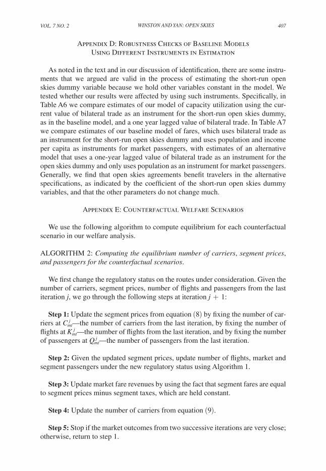
VOL. 7 NO. 2 407WINSTON AND YAN: OPEN SKIES
Appendix D: Robustness Checks of Baseline Models Using Different Instruments in Estimation
As noted in the text and in our discussion of identification, there are some instru-ments that we argued are valid in the process of estimating the short-run open skies dummy variable because we hold other variables constant in the model. We tested whether our results were affected by using such instruments. Specifically, in Table A6 we compare estimates of our model of capacity utilization using the cur-rent value of bilateral trade as an instrument for the short-run open skies dummy, as in the baseline model, and a one year lagged value of bilateral trade. In Table A7 we compare estimates of our baseline model of fares, which uses bilateral trade as an instrument for the short-run open skies dummy and uses population and income per capita as instruments for market passengers, with estimates of an alternative model that uses a one-year lagged value of bilateral trade as an instrument for the open skies dummy and only uses population as an instrument for market passengers. Generally, we find that open skies agreements benefit travelers in the alternative specifications, as indicated by the coefficient of the short-run open skies dummy variables, and that the other parameters do not change much.
Appendix E: Counterfactual Welfare Scenarios
We use the following algorithm to compute equilibrium for each counterfactual scenario in our welfare analysis.
ALGORITHM 2: Computing the equilibrium number of carriers, segment prices, and passengers for the counterfactual scenarios.
We first change the regulatory status on the routes under consideration. Given the number of carriers, segment prices, number of flights and passengers from the last iteration j , we go through the following steps at iteration j + 1 :
Step 1: Update the segment prices from equation (8) by fixing the number of car-riers at C mt j —the number of carriers from the last iteration, by fixing the number of flights at K mt j —the number of flights from the last iteration, and by fixing the number of passengers at Q mt j —the number of passengers from the last iteration.
Step 2: Given the updated segment prices, update number of flights, market and segment passengers under the new regulatory status using Algorithm 1.
Step 3: Update market fare revenues by using the fact that segment fares are equal to segment prices minus segment taxes, which are held constant.
Step 4: Update the number of carriers from equation (9).
Step 5: Stop if the market outcomes from two successive iterations are very close; otherwise, return to step 1.

408 AMERICAN ECONOMIC JOURNAL: ECONOMIC POLICY MAY 2015
Appendix: Tables
Table A1—Regression Tests of the Instruments in the Bottom-Level Demand Equations
Dependent variable: log air fare
of segment 1
Dependent variable: log air fare
of segment 2Dependent variable: log real expenditurea
Instrumental variables (1) (2) (3)
Panel A. Full sample (22,638 observations for each specification)Demeaned log tax per person of segment 1 0.1573 (0.0068)Demeaned log tax per person of segment 2 0.4641 (0.0085)Demeaned log geometric mean population of the end-point countries
1.2954 (0.2931)
Demeaned log geometric mean income per capita of the end-point countries
0.3437 (0.0551)
Instruments for other endogenous variables and exogenous regressors included?
Yes Yes Yes
Panel B. US international routes only (3,766 observations for each specification)Demeaned log tax per person of segment 1 0.4192 (0.0194)Demeaned log tax per person of segment 2 0.4923 (0.0162)Demeaned log geometric mean population of the end-point countries
6.2845 (1.9127)
Demeaned log geometric mean income per capita of the end-point countries
0.5336 (0.2123)
Instruments for other endogenous variables and exogenous regressors included?
Yes Yes Yes
Note: Numbers in parentheses are standard errors.a Real expenditure is constructed by using equation (2) in the text and GMM estimates of the parameters.
Table A2—Regression Tests of the Instruments in the Top-Level Demand Equation
Dependent variable: market price indexa
Dependent variable: log flight frequency
(number of flights)
Dependent variable: log geometric mean
population of the end-point countries
Dependent variable: log geometric mean income per capita of
the end-point countriesInstrumental variables (1) (2) (3) (4)
Panel A. Full sample (17,572 observations for each specification)Demeaned average tax per person across segments
0.0066 (0.0002)
Demeaned log geometric mean population of the end-point countries
0.8181 (0.3321)
Demeaned log geometric mean income per capita of the end-point countries
0.9825 (0.0059)
Demeaned first-difference of one year lag log flight frequency
0.2229 (0.0164)
Panel B. US international routes only (2,940 observations for each specification)Demeaned average tax per person across segments
0.0046 (0.0005)
Demeaned log geometric mean population of the end-point countries
0.9472 (0.0040)
Demeaned log geometric mean income per capita of the end-point countries
0.9948 (0.0013)
Demeaned first-difference of one year lag log flight frequency
0.2047 (0.0316)
Instruments for other endogenous variables and exogenous regressors included?
Yes Yes Yes Yes
Note: Numbers in parentheses are standard errors.a Price index is constructed by using equation (2) in the text and GMM estimates of the parameters.

VOL. 7 NO. 2 409WINSTON AND YAN: OPEN SKIES
Table A3—Regression Tests of Bilateral Trade as the Instrument for the Short-Run Open Skies Dummy in the Equilibrium Capacity Utilization Equation and Segment Fare Equationsa
Dependent variable: the short-run
open skies dummy
Dependent variable: the short-run
open skies dummyInstrumental variables (1) (2)Panel A. Full sampleDemeaned monthly trade value between the end-point countries 0.0059 (0.0002)Demeaned one-year lag of monthly trade value between the end-point countries
0.0041 (0.0003)
Observations 22,638 18,019
Panel B. US international routes onlyDemeaned monthly trade value between the end-point countries 0.0102 (0.0004)Demeaned one-year lag of monthly trade value between the end-point countries
0.0097 (0.0006)
Observations 3,766 3,009
Note: Numbers in parentheses are standard errors.a Instruments for other endogenous variables and exogenous regressors in equilibrium capacity utilization equa-
tion and segment fare equations are included in all estimations.
Table A4—Testing Cointegration between log Number of Market Passengers and log Number of Flights Based on Regression Equation (11) in the Text
Variables (1) (2) (3)Panel A. Full sample e ̂ m (t−1) −0.4569 −0.4014 −0.3426
(0.0051) (0.0059) (0.0114)
{Δ e ̂ m (t−j) } j=1
p Not included Included and p = 1 Included and p = 15
X ˜ mt (including year and month dummies) Not included Included Included
Overall R2 0.04 0.03 0.04
Observations 25,849 24,988 18,389
Panel B. US international routes only e ̂ m (t−1) −0.6059 −0.5614 −0.5294
(0.0143) (0.0172) (0.0369)
{Δ e ̂ m (t−j) } j=1
p Not included Included and p = 1 Included and p = 15
X ˜ mt (including year and month dummies) Not included Included Included
Overall R2 0.08 0.01 0.05
Observations 4,141 4,067 3,067
Note: Numbers in parentheses are standard errors.

410 AMERICAN ECONOMIC JOURNAL: ECONOMIC POLICY MAY 2015
Table A5—Robustness Check: GMM Estimates of Equilibrium Capacity Utilization (US international routes only)
Baseline results: Model 4 of Table 6 in the text
using demeaned bilateral trade value as the
instrument for short-run open skies dummy(standard errors)
(1)
Using demeaned one-year lag
of bilateral trade value as the instrument
for short-run open skies dummy(standard errors)
(2)
log number of market passengers in a month 0.6825(0.0203)
0.6785(0.0225)
Short-run open skies dummy (1 if an OS agreement was signed after 2005; 0 otherwise)
0.1605(0.0534)
0.1885(0.0818)
Long-run open skies dummy (1 if an OS agreement was signed before 2000; 0 otherwise)
−0.0026(0.3441)
0.0403(0.0397)
log geometric mean population of the end-point countries 2.2522(1.2726)
2.2382(1.7099)
log geometric mean of income per capita of the end-point countries
0.2598(0.1734)
0.3897(0.2241)
log number of carriers 0.0999(0.0337)
0.1150(0.0378)
Presence of an airline alliance 0.0324(0.0523)
0.0548(0.0577)
log distance −0.4946(0.0175)
−0.5101(0.0191)
log number of cities connected to the end-point airports 0.8522(0.0408)
0.8778(0.0445)
Maximal historical average rainfall at the end-point cities in a montha
−0.3864(0.0915)
−0.3425(0.1007)
Maximal temperature difference between January and July at the end-point citiesb
−0.0135(0.0012)
−0.0124(0.0013)
Regional dummies included Yes YesCountry dummies included Yes YesYear dummies included Yes YesMonth dummies included Yes YesRandom market effects taken into account Yes YesNumber of markets (nondirectional routes) 66 66
Observations 3,766 3,009
a This variable is measured as the maximal value of the historical average monthly rainfall (000’s mm) at the two end-point cities. Data were obtained from airport websites.
b This variable is measured as the maximal value of the difference in the average temperature between July and January at the two end-point cities. Data were obtained from airport websites.

VOL. 7 NO. 2 411WINSTON AND YAN: OPEN SKIES
Table A6—Robustness Check: GMM Estimates of the Fare Equations (US international routes only)a
log fare of segment 1 (business plus)
(1)
log fare of segment 2 (economy full)
(2)
log fare of segment 3 (economy discount or other)
(3)
Panel A. Baseline results presented in Table 8 of the text using demeaned bilateral trade value as the instrument for the short-run open skies dummy and using both geometric mean population and income per capita of end-point countries as instruments for log number of market passengersShort-run open skies dummy −0.4886 (0.0456) −0.2621 (0.0375) −0.2476 (0.0436)Long-run open skies dummy −0.2509 (0.0480) −0.2058 (0.0412) −0.2412 (0.0448)log number of market passengers in a month
0.2945 (0.1043) 0.3121 (0.1009) 0.5715 (0.1278)
Capacity utilizationb −0.0163 (0.0210) −0.0046 (0.0188) 0.0157 (0.0273)log number of carriers −0.0798 (0.0412) −0.0411 (0.0392) −0.1378 (0.0515)log distance 0.2943 (0.0309) 0.0820 (0.0315) 0.1609 (0.0424)log distance × crude oil price 0.0961 (0.0226) 0.0928 (0.0229) 0.0783 (0.0301)Presence of an airline alliance −0.2050 (0.0514) −0.1059 (0.0538) −0.2641 (0.0770)Maximal historical average monthly rainfall between the end-point citiesc
0.1712 (0.1200) 0.2102 (0.1223) 0.3202 (0.1512)
Maximal temperature difference between January and July at the end-point citiesd
0.0224 (0.0016) 0.0176 (0.0014) 0.0146 (0.0019)
Number of markets (routes) 66 66 66
Observations 3,766 3,766 3,766
Panel B. Using demeaned one-year lag of bilateral trade value as the instrument for the short-run open skies dummy; using only geometric mean population of end-point countries as the instrument for log number of market passengersShort-run open skies dummy −0.2248 (0.0840) −0.2466 (0.0693) −0.3925 (0.1118)Long-run open skies dummy −0.2033 (0.0558) −0.3190 (0.0485) −0.3565 (0.0811)log number of market passengers in a month
0.2210 (0.1982) 0.0822 (0.2235) 0.7874 (0.3381)
Capacity utilizationb 0.0127 (0.0208) 0.0201 (0.0198) 0.0324 (0.0402)log number of carriers −0.0934 (0.0628) 0.0396 (0.0657) −0.1861 (0.1082)log distance 0.2822 (0.0351) 0.0493 (0.0352) 0.1551 (0.0613)log distance × crude oil price 0.0919 (0.0223) 0.1158 (0.0221) 0.0840 (0.0394)Presence of an airline alliance −0.1149 (0.0484) 0.0077 (0.0513) −0.2123 (0.1125)Maximal historical average monthly rainfall between the end-point citiesc
0.1129 (0.2001) 0.0035 (0.2251) 0.5756 (0.3451)
Maximal temperature difference between January and July at the end-point citiesd
0.0204 (0.0022) 0.0139 (0.0024) 0.0156 (0.0038)
Number of markets (routes) 66 66 66
Observations 3,009 3,009 3,009
a Region, country, year, and month fixed effects are included in all the regressions. Numbers in parentheses are standard errors.
b Capacity utilization is constructed by log ( K mt ) − 0.6174 log ( Q mt ) in the full sample and log ( K mt ) − 0.6825 log ( Q mt ) in the US subsample.
c This variable is measured as the maximal value of the historical average monthly rainfall (000’s mm) at the two end-point cities. Data were obtained from airport websites.
d This variable is measured as the maximal value of the difference in the average temperature between July and January at the two end-point cities. Data were obtained from airport websites.

412 AMERICAN ECONOMIC JOURNAL: ECONOMIC POLICY MAY 2015
Table A7—US International Routes with Open Skies Agreements Signed between January 1, 2005 and December 31, 2009*
Origin DestinationOrigin country
Destination country
Year/month of signing OSA
Boston London Heathrow United States United Kingdom 2007/04Newark London Heathrow United States United Kingdom 2007/04Washington Dulles London Heathrow United States United Kingdom 2007/04New York (JFK) London Heathrow United States United Kingdom 2007/04Los Angeles London Heathrow United States United Kingdom 2007/04Las Vegas London Gatwick United States United Kingdom 2007/04London Heathrow Miami United Kingdom United States 2007/04London Heathrow Chicago O’Hare United Kingdom United States 2007/04London Heathrow San Francisco United Kingdom United States 2007/04London Gatwick Orlando United Kingdom United States 2007/04Manchester Orlando United Kingdom United States 2007/04Dublin (DUB) New York (JFK) Ireland United States 2007/04New York (JFK) Madrid United States Spain 2007/04Los Angeles Sydney United States Australia 2008/02Newark Toronto United States Canada 2007/03Fort Lauderdale Toronto United States Canada 2007/03Las Vegas Toronto United States Canada 2007/03Los Angeles Toronto United States Canada 2007/03New York (LGA) Toronto United States Canada 2007/03Orlando Toronto United States Canada 2007/03Miami Toronto United States Canada 2007/03Chicago O’Hare Toronto United States Canada 2007/03Las Vegas Vancouver United States Canada 2007/03Los Angeles Vancouver United States Canada 2007/03San Francisco Vancouver United States Canada 2007/03Fort Lauderdale Montreal United States Canada 2007/03
* The United States signed an open skies agreement with Japan at the end of 2010. The 26 routes consist of 5 country pairs.
Table A8—US International Routes Governed by Open Skies Agreements before 2000a
Origin Destination Origin country Destination country
Amsterdam New York (JFK) Netherlands United StatesRome New York (JFK) Italy United StatesFrankfurt New York (JFK) Germany United StatesFrankfurt San Francisco Germany United StatesIncheon New York (JFK) South Korea United StatesIncheon Los Angeles South Korea United StatesIncheon San Francisco South Korea United StatesNew York (JFK) Milan United States ItalyLos Angeles Taipei United States TaiwanLima Miami Peru United StatesSan Francisco Taipei United States Taiwan
a The 11 routes consist of 6 country pairs.

VOL. 7 NO. 2 413WINSTON AND YAN: OPEN SKIES
REFERENCES
Barnhart, Cynthia, and Amy Cohn. 2004. “Airline Schedule Planning: Accomplishments and Oppor-tunities.” Manufacturing and Service Operations Management 6 (1): 3–22.
Belobaba, Peter, Amadeo Odoni, and Cynthia Barnhart, eds. 2009. The Global Airline Industry. New York: John Wiley.
Berry, Steven, and Panle Jia. 2010. “Tracing the Woes: An Empirical Analysis of the Airline Industry.” American Economic Journal: Microeconomics 2 (3): 1–43.
Brueckner, Jan K. 2001. “The Economics of International Codesharing: An Analysis of Airline Alli-ances.” International Journal of Industrial Organization 19 (10): 1475–98.
Brueckner, Jan K., Darin N. Lee, and Ethan S. Singer. 2011. “Alliances, Codesharing, Antitrust Immu-nity, and International Airfares: Do Previous Patterns Persist?” Journal of Competition Law and Economics 7 (3): 573–602.
Cilberto, Federico, and Elie Tamer. 2009. “Market Structure and Multiple Equilibria in Airline Mar-kets.” Econometrica 77 (6): 1791–1828.
Cristea, Anca, David Hummels, and Brian Roberson. 2012. “Estimating the Gains from Liberaliz-ing Services Trade: The Case of Passenger Aviation.” http://economics.yale.edu/sites/default/files/hummels-130403.pdf.
Deaton, Angus, and John Muellbauer. 1980. “An Almost Ideal Demand System.” American Economic Review 70 (3): 312–26.
Gillen, David W., William G. Morrison, and Christopher Stewart. 2003. Air Travel Demand Elastic-ities: Concepts, Issues and Measurement. Canadian Department of Finance. http://www.fin.gc.ca/consultresp/airtravel/airtravstdy_-eng.asp.
Table A9—US International Routes Not Governed by Open Skies Agreements as of December 31, 2009*
Origin Destination Origin country Destination country
Bogotá Miami Colombia United StatesCaracas Miami Venezuela United StatesCancun New York (JFK) Mexico United StatesCancun Miami Mexico United StatesNewark Tel Aviv United States IsraelBuenos Aires Miami Argentina United StatesFort Lauderdale Kingston United States JamaicaGuadalajara Los Angeles Mexico United StatesSão Paulo New York (JFK) Brazil United StatesSão Paulo Miami Brazil United StatesHong Kong New York (JFK) Hong Kong United StatesHong Kong Los Angeles Hong Kong United StatesHong Kong San Francisco Hong Kong United StatesHonolulu Kansai United States JapanHonolulu Tokyo Narita United States JapanNew York (JFK) Mexico City United States MexicoNew York (JFK) Tokyo Narita United States JapanNew York (JFK) Piarco United States Trinidad and TobagoNew York (JFK) Santo Domingo United States Dominican RepublicNew York (JFK) Santiago United States Dominican RepublicNew York (JFK) Tel Aviv United States IsraelLos Angeles Mexico City United States MexicoLos Angeles Manila United States PhilippinesLos Angeles Tokyo Narita United States JapanMexico City Miami Mexico United StatesMiami Port-au-Prince United States HaitiMiami Santo Domingo United States Dominican RepublicMiami San José United States Costa RicaTokyo Narita San Francisco Japan United States
* The United States signed an open skies agreement with Japan at the end of 2010. The 29 routes consist of 15 country pairs.

414 AMERICAN ECONOMIC JOURNAL: ECONOMIC POLICY MAY 2015
Hausman, Jerry A. 1996. “Valuation of New Goods under Perfect and Imperfect Competition.” In The Economics of New Goods, Vol. 58, edited by Timothy F. Bresnahan and Robert J. Gordon, 209–37. Chicago: University of Chicago Press.
Hausman, Jerry A., and William E. Taylor. 1981. “Panel Data and Unobservable Individual Effects.” Econometrica 49 (6): 1377–98.
Joskow, Paul L., and Nancy L. Rose. 1989. “The effects of economic regulation.” In Handbook of Industrial Organization, Vol. 2, edited by Richard Schmalensee and Robert Willig, 1449–1506. Amsterdam: North-Holland.
Ke, Jian-yu, and Robert J. Windle. 2012. “The Ongoing Impact of the U.S.-China Air Services Agree-ments.” Unpublished.
Micco, Alejandro, and Tomás Serebrisky. 2006. “Competition Regimes and Air Transport Costs: The Effects of Open Skies Agreements.” Journal of International Economics 70 (1): 25–51.
Morrison, Steven A., and Clifford Winston. 1986. The Economic Effects of Airline Deregulation. Washington, DC: Brookings Institution Press.
Morrison, Steven A., and Clifford Winston. 1995. The Evolution of the Airline Industry. Washington, DC: Brookings Institution Press.
Morrison, Steven A., and Clifford Winston. 2000. “The Remaining Role of Government Policy in the Deregulated Airline Industry.” In Deregulation of Network Industries: What’s Next? edited by Sam Peltzman and Clifford Winston, 1–40. Washington, DC: Brookings Institution Press.
Piermartini, Roberta, and Linda Rousová. 2013. “The Sky is not Flat: How Discriminatory is the Access to International Air Services?” American Economic Journal: Economic Policy 5 (3): 287–319.
Poole, Jennifer Pamela. 2013. “Business Travel as an Input to International Trade.” Unpublished.Whalen, W. Tom. 2007. “A panel data analysis of code sharing, antitrust immunity, and open skies trea-
ties in international aviation markets.” Review of Industrial Organization 30 (1): 39–61. Winston, Clifford. 2013. “On the Performance of the U.S. Transportation System: Caution Ahead.”
Journal of Economic Literature 51 (3): 773–824.Winston, Clifford, and Jia Yan. 2015. “Open Skies: Estimating Travelers’ Benefits from Free Trade
in Airline Services: Dataset.” American Economic Journal: Economic Policy. http://dx.doi.org/10.1257/pol.20130071.