Open | Models Laboratory - OMiLABvienna.omilab.org/repo/files/Bee-Up/The_IMKER_Case_Study.pdf ·...
56
Open | Models Laboratory The “IMKER” Case Study Practice with the Bee-Up tool Dimitris Karagiannis Patrik Burzynski Elena-Teodora Miron
Transcript of Open | Models Laboratory - OMiLABvienna.omilab.org/repo/files/Bee-Up/The_IMKER_Case_Study.pdf ·...

O p e n | M o d e l s
Laboratory
The “IMKER” Case StudyPractice with the Bee-Up tool
Dimitris Karagiannis
Patrik Burzynski
Elena-Teodora Miron

Main Authors
Dimitris Karagiannis
Patrik Burzynski
Elena‐Teodora Miron
March 2017
The IMKER case study
1
Bee‐Up: A Multi‐language Modeling Environment for Design and Evaluation of
Conceptual Models
The IMKER case study Abstract
Conceptual modelling is a technique which is essential for building enterprise information systems. The
reason is not only because software systems have to be built, but also since domain specific
requirements coming from the application area should be represented adequately. For this reason
different modelling languages for data modelling, process modelling and systems modelling are
developed. In this case study we deal with the fundamental conceptual modelling languages, like BPMN,
EPC, ER, UML and Petri Nets. A tool support through Bee‐Up is also given (www.omilab.org). This case
study focuses on the domain of beekeeping throughout different areas, like the production of honey,
bees in general and beekeepers (called Imker in German).
Table of Contents
The IMKER case study .................................................................................................................................. 1
1. The IMKER World ................................................................................................................................. 2
2. Settings ................................................................................................................................................. 3
3. Model Extraction and Design ............................................................................................................... 4
4. Modelling Languages: Overview .......................................................................................................... 6
5. A Specific Case .................................................................................................................................... 11
6. The Bee‐Up Environment ................................................................................................................... 16
Appendix I: Bee‐Up Handbook ................................................................................................................... 28
1. General information ........................................................................................................................... 28
2. Installation .......................................................................................................................................... 28
3. Modelling with the Bee‐Up tool ......................................................................................................... 32
4. Exporting models ................................................................................................................................ 37
5. Additional hints and information ....................................................................................................... 39
6. Change History ................................................................................................................................... 51
7. Development Team ............................................................................................................................ 52
8. Additional used Tools ......................................................................................................................... 52

The IMKER case study
2
1. The IMKER World Bees might be known to many as a nuisance, especially during a picnic, but they also
provide different products and services used in different areas of life, of which honey is
probably the best known. In 2015 the honey production yielded ~268 thousand tons of
honey in the European Union, being the second largest honey producer after China.
However, the EU was also the largest importer of honey in 2015, with ~198 thousand
tons of imported honey, at ~2520 euro per ton, while only exporting ~18 thousand tons, at ~5770 euro
per ton. Nevertheless the honey market is considered small in the EU compared to its other markets.
Besides honey bees also provide beeswax, which can be used for candles, in cosmetic products or
pharmaceuticals. Another product provided by bees is propolis with applications in naturopathic
treatments.
Bees also play an important role in pollination of crops and other plants, which is
necessary for their reproduction. It is estimated that 90% of pollination is achieved
through biotic pollination, where living organisms move the pollen from plant to plant.
It is estimated that biotic pollination contributes 22 billion euros to the European
agriculture industry each year. While plants are pollinated by many different insects,
including flies, beetles and butterflies, the managed nature of bees through beekeeping helps
intentionally pollinate specific fields, growing for example sunflowers.
Beekeeping, or apiculture, is the intentional management of bees, often for the
purpose of producing the different products of bees, the breeding of bees, and
pollination of plants. To be able to manage the bees or rather an entire bee colony a
beehive (or simply hive) is used. In 2015 the total number of hives in the European
Union was estimated at 16 million. Beehives are often built out of several different
parts, serving different functions, not only to provide a home to a bee colony, but also to facilitate the
work of a beekeeper, like extracting the honey or protecting the bees against rodents.
A beekeeper, called Imker in German, takes care of their bees and their hive and
harvests the different products of the bees or provides a pollination service. In the
previous years the number of beekeepers has been decreasing in the EU, reaching
~600 thousand beekeepers in 2015. Generally beekeepers can be mainly categorized
in commercial and recreational, which practice beekeeping as a hobby. To go about
their work the beekeeper also has different tools at their disposal, like a bee smoker to calm the bees,
special protective attire or a honey extractor. While a beekeeper is capable of managing the colonies
and influence them to a certain degree, they cannot directly control the bees. It is a beekeepers task to
take care and help the colonies under their care.
The beekeepers are themselves receiving help from different organization. The
European Union is supporting beekeeping through different apiculture programs,
funding 216 million euros (50% from the EU, 50% from member states) in the period of
2017 to 2019. It has also created regulations to provide a legal basis for establishing a
common organization of the markets in agricultural products, to which honey belongs.
Additionally national beekeeping associations (e.g. The British Beekeepers Association, Österreichischer
Imkerbund etc.) provide varying services for the beekeepers and interested people alike, for example
education of the general population, specific courses for beekeepers to extend their knowledge, funding
of beekeepers, support with legal aspects like insurance or registration or web‐shops providing items for
beekeepers and interested people alike. There are of course also legal obligations for beekeeping and
beekeepers, which can differ from country to country. For example the EU has specific labelling rules for
honey.

The IMKER case study
3
Sources for the IMKER World (accessed 19.01.2017):
https://ec.europa.eu/agriculture/honey_en https://ec.europa.eu/agriculture/sites/agriculture/files/honey/presentation‐honey‐2015_en.pdf http://ec.europa.eu/agriculture/sites/agriculture/files/evaluation/market‐and‐income‐
reports/2013/apiculture/chap3_en.pdf
https://ec.europa.eu/agriculture/honey/programmes_en
http://eur‐lex.europa.eu/legal‐content/en/TXT/?qid=1475150583359&uri=CELEX:32013R1308 http://ec.europa.eu/food/animals/live_animals/bees_en
http://www.ecpa.eu/sites/default/files/Pollinators%20brochure_B%C3%A0T2.pdf http://www.bbka.org.uk/ https://www.imkerbund.at
http://www.beverlybees.com/parts‐beehive‐beginner‐beekeeper/
http://eur‐lex.europa.eu/legal‐content/EN/TXT/?uri=URISERV%3Al21124a
2. Settings The domain of beekeeping provides different settings where information technology and conceptual
models can be applied, of which some will be presented in the following paragraphs.
A commercial beekeeper thinks to revise the approach of how they currently make money. They
consider using a Business model for this purpose. A Business model describes the setting of a business
and how it aims to achieve its goals and can be used to describe the currently applied approach or
possible alternatives. One form for modelling the business is through its business processes, where the
tasks providing the desired effect as well as any relevant preceding tasks and partners participating in
the execution can be described. This also helps to identify tasks that can further be supported by
information technology or use information technology to transform the business model all together.
Business processes can be described using the Business Process Model and Notation (BPMN).
A company employing several beekeepers aims to better manage its resources and business processes
and plans to achieve this by introducing an Enterprise Resource Planning (ERP) system. An ERP system
allows managing the different resources found in a company, allowing varying views for different
functions on the same data. The available functions and the possibility for their extension depend on the
chosen ERP implementation, like standard software possibly with customization options or an in‐house
developed ERP system. The functions can focus for example on analytics, finance, human resources,
supply chains or (business) process management. Different types of models can be employed to
customize an ERP system, but as a specific example Event‐driven Process Chains (EPC) can be utilized for
process management.
A beekeeper, which is currently selling their goods in local shops, wants to reach a wider range of
customers. For this they consider providing an e‐shop. An e‐shop allows changing the behavior of
purchasing goods, providing benefits for different actors, for example for selling honey, bred queen
bees, equipment for beekeepers or pollination services to field owners. An e‐shop changes the typical
synchronous handling of purchases in a store to an asynchronous one and also allows for a geographical
difference between the customer and the provider when purchasing products or at least placing orders.
Additionally it requires providing a catalogue describing the products/services provided to the customer.
To offer a maintainable e‐shop solution a proper data structure is required. This data structure can be
designed using Entity Relationship models (ER), which can be processed to implement a database.
A new start‐up enterprise wants to introduce “smart factory” practices into beekeeping, like automated
harvesting and maintaining of beehives or automatically retrieval of hives using for example mechanical
drones. A smart factory, a part of Industry 4.0, introduces special principles into manufacturing and the
use of certain technology, most notably the integration of the Internet of Things (IoT) and use of Cyber‐

The IMKER case study
4
Physical Systems (CPS). Some of the identified principles are interconnection between the actors,
information transparency and decentralized decisions. A smart factory uses information from both the
physical and the virtual world to assist the execution of manual or automated tasks. To design and
describe specific scenarios that can then be implemented in a smart factory a modelling language for
describing the different aspects of systems like the Unified Modeling Language (UML) is necessary.
An enterprise focusing on the production of different bee‐related products wants to go green and thus
to analyze their production processes according to the idea of “Green Production”. Green Production is
a strategy that incorporates environmental concerns into the processes and redesign of products to
reduce the negative impact on the environment. Environmental concerns to be considered are for
example the pollution during the production, the use of raw materials and the amount or use of created
waste, in order to achieve an environmentally sustainable state. In this setting Petri Nets can be used for
modelling and analyzing the production processes according to the previously stated aspects. For
example Petri Nets can be employed to identify tasks producing waste and considering how to reduce
waste or maybe even reuse the waste as material.
The described settings serve the general understanding for the application of conceptual models with
different modelling languages. Specific examples can be found in section 5.1.
3. Model Extraction and Design Based on information gathered from the IMKER World, a selected case in section 5 is designed that is
relevant for current, or just beyond current, individual student practice within conceptual models. Based
on the goal and desired outcome, the proper modelling languages and modelling approach has to be
chosen. However, independent of those there are three general steps that have to take place.
In the first step reading and understanding within a “text annotation approach” has to
take place, resulting in a number of design alternatives. Annotation of text allows
identifying the relevant information to fulfil the modelling requirements for a specific
case. Text annotations provide additional information to the reader through different
means of enhancing the text. This can be achieved through simple forms, like changes
in the text‐format or highlighting the text, or by adding content in the form of footnotes, comments or
links. Annotations providing additional content allow clarifying certain parts without requiring the
change the original text. The annotation of text can benefit different cases, like utilizing notes for a
specific reader's purpose in form of private annotations, public annotations viewable by all readers or
annotations supporting the collaboration of different authors during the writing of a text.
When modelling individually instead of in a workshop environment, it is suggested to use this approach
to identify the main concepts which have to be modelled. We use the annotation techniques to identify
relevant modelling concepts for a specific purpose. It is desirable that the individual implementing the
scenario will define the information for the model building process according to their understanding and
their view.
The OMiLAB Bee‐Up page provides an online annotation tool for this case study. It can be accessed at
http://www.omilab.org/bee‐up. For a general purpose annotation tool you can try SCRIBLE©.
The next step is a cognitive task, namely “mapping” the domain specifics within the
modelling languages concepts. This requires knowledge about the specific case that
has to be modelled and its domain, which should have been obtained from the
previously annotated text, as well as knowledge about the used modelling language
and the domain the model will be utilized in. The focus ought to be on deciding what
should be and how it should be depicted in the model. Here the student has to apply modeling language
knowledge and domain characteristics on an abstraction level, using the appropriate modeling
language‐elements and ‐rules.

The IMKER case study
5
Finally, the model design has to take place based on the specific scenarios, applying
the elements of the chosen modelling language and designing the semantical and
syntactical structure to create a conceptual model. Using the knowledge about the
domains and the modelling language and the mapping between the main concepts and
model elements allows creating the desired model. The detail of the model depends
also on how profound the knowledge of the modelling language is. Here the attention should be
directed towards how and in what relation to one another the things should be depicted. Traditionally,
model design refers to students writing several versions of a model, improving each version on the basis
of feedback from the teacher or from peers.
Different tools supporting the creation of model are available, ranging from simple pen and paper to
fully integrated modelling applications. In this case the exercises should be solved using the functionality
of the Bee‐Up conceptual modeling tool (see Appendix I). The primary reason for that is because we use
transformation and generation algorithms, like generating SQL from Entity Relationship models or RDF
descriptions from models. A conceptual modeling tool like Bee‐Up could give immediate support and
help in a feedback cycle to improve also the quality of the model.
Bee‐Up modeler is the tool that is used in this case study.
The conceptual models for the case will be extracted with the following process steps: annotate –
mapping – design.
Figure 1: An interactive model extraction and design procedure
It is envisaged that a student builds collaboratively shared models on a topic related to his/her exercises,
possibly with collaborating students from different disciplines. This will increase the involvement of
domain experts and consequently the model quality.
Bee‐Up Wiki should help here with IMKER content.
Because research indicates that students learn more from feedback given during the working process
rather than after, it is also planned to implement a feedback component.

The IMKER case study
6
4. Modelling Languages: Overview Business Process Model and Notation (BPMN) is an OMG standard designed to support the business
process management paradigm with a more extensive range of diagrammatic possibilities compared to
traditional flowcharts or UML activity diagrams. The language allows the modelling of individual or
collaborative processes using the main concepts of Participants reacting to Events and performing Tasks,
whose flow can be controlled through Gateways. The support for the business process management
paradigm is achieved by adding domain‐specificity in the languages semantics manifested through a
richness of types for different concepts (Tasks, Events, Gateways). Additionally, due to the strong focus
on notation, this variability in semantics is also reflected in the visualization of the concepts by adding
visual cues to the shapes.
Event‐driven Process Chain (EPC) diagrams were introduced by the framework of Architecture of
Integrated Information Systems (ARIS) and its software tools. The main concepts are Events and
Functions depicting an alternating flow between “states” and “changes” to those states. The Functions
can further be connected to other elements of the enterprise context (responsible organization unit,
supporting IT system, input/output information). While the target domain of BPMN is shared by EPC the
exact scope is different, having a distinct trade‐off between understandability and underlying formal
rigor through color coding and shape coding of concepts while removing the rich taxonomical
classifications promoted by BPMN.

The IMKER case study
7
Entity‐Relationship (ER) models have been widely adopted in the conceptual modelling community as
the fundamental approach for data modelling, especially for the design and data schema generation of
databases. The core concepts are the Entity, the Relationship between Entities and the Attributes of
Entities and Relationships. Dealing with Entities rather than tables/tuples an ER model may describe
data to be stored in structures other than relational databases. By describing categories of being and
their relations an ER model has a similar scope to UML Class Diagrams or meta‐models.
Unified Modeling Language (UML) is one of the most prominent standards in software engineering
aimed at supporting a unified method for object‐oriented software development. To achieve this it
incorporates lessons learned from a large number of previously used modelling languages and through
covering a wide scope using different diagram types addressing various aspects of a software system.
Those diagram types care categorized into structural diagrams showing the static structure of objects in
a system (e.g. Class Diagram, Component Diagram …) and behavioral diagrams describing the dynamic
behavior of objects in a system (e.g. Use Case Diagram, Activity Diagram …). UML Profiles and
Stereotypes further allow a certain degree of customization of the language. UML may be seen as a
natural descendant of the simpler and more focused ER modelling approach. While it shares ER’s
desideratum of code generation, it focuses on an object‐oriented development context (e.g. class
definitions derived from class diagrams).

The IMKER case study
8
Petri Nets (PN) is one of the longest standing diagrammatic modeling methods, with minimal but
powerful semantics based on strong mathematical foundations. The core concepts are Places (states),
Transitions (changes, actions) and Arcs (indicating the flow) as well as Tokens (marks) which capture the
behavioral dynamics of a system. The firing (execution) of Transitions signify an action taken by passing
the Tokens between their adjacent Places according to the defined flow. While the method is sufficiently
abstract to have cross‐domain applicability with respect to process dynamics, it imposes however a
learning curve that is typically not acceptable for business stakeholders. Simulation mechanisms,
monitoring the possible states of the system as a whole through the firing of Transitions and movement
of Tokens (Token availability in a selected Place will enable the Transitions following that Place), are
employed to assess the reachability of certain states, the risk of deadlock and the liveness/deadness of
certain transitions.
4.1 Selected Modelling Examples The following section contains some examples showing how certain cases can be modelled.
4.1.1 Process of registration for NEMO Summer School This example from the NEMO Summer School 2016 illustrates how the process of registration can be
modeled using BPMN.
Process description: Students interested in participating at the NEMO Summer School are required to
submit an application. Thus when starting the application process the student must procure a
recommendation letter, write a motivation letter and compose her/his CV. Then she/he needs to fill out
the application form. Within the application form the student must indicate whether she/he is applying
for financial aid or not. Before submitting the application the student attaches the three documents
mentioned above. When the application has been submitted the NEMO administrative staff receives a
notification e‐mail that a new registration has been included in the database. The staff writes an e‐mail
to the student confirming the receipt of the application. Subsequently the staff checks whether the
application is complete. If the application is complete the documents are printed and put in a file in
order to be handed to the selection committee. If any information/document is missing the student is
contacted via e‐mail and requested to provide the missing information/document within the next 2
weeks. After 2 weeks the NEMO administrative staff checks if the outstanding information/document
has been received. If the information has not been provided by the student or is still incomplete the
staff writes an e‐mail informing the applicant that her/his application has been denied due to the failure
to provide a complete application file. The submitted documents and the rejection e‐mail are archived
and the process ends. If the student has provided the requested information the documents are printed
and put in a file in order to be handed to the selection committee. The application documents are
complete in 90% of cases. In 5% of the cases the student fails to provide the requested
information/documents.

The IMKER case study
9

The IMKER case study
10
4.1.2 Data model for NEMO Summer School information system This example from the NEMO Summer School 2016 illustrates how the requirements for an information
system can be used to model the data structure using an ER model.
Requirements: Participants at the summer school are either students or teachers. Each student registers
for the NEMO Summer School providing, amongst others, their level of study (Bachelor, Master or PhD)
and their field of study. Additionally each student provides her/his first name, last name, their country
of provenience and e‐mail address. Students attend courses during the summer school. Courses can be
a lecture, a fundamentals exercise or application exercises. [The fundamental exercise is considered as
one unit as it covers one topic, although it takes place in several sessions.] Each course has a title, is
being given by one or more lecturers and takes places in a room. Every room has a name, a seating
capacity, and technical equipment. Lectures and application exercises take place in a lecture hall, while
fundamental exercises are conducted in PC‐labs. Within the fundamentals exercise students are split in
groups. Each group has a group number, a room (i.e. PC‐lab) and a tutor. Teachers can be either
lecturers or tutors. Each teacher has a first name, last name, host institution, and country.

The IMKER case study
11
5. A Specific Case Consider the text below to be the transcript of an interview with a beekeeper1. While the interviewer
might direct the conversations at times, the actual questions are omitted and only the information from
the beekeeper is kept.
Paragraph 1: As a beekeeper I currently tend to five hives spread across two apiaries. I put all of my
hives in places I can get to with my car, since they can be quite heavy and it is easier to move them with
my pickup truck from one apiary to a different one or back to the tool‐shed to perform some repairs.
Currently I have three hives between Sherwood Forest and McJenkins field, Sherwood Forest being west
and McJenkins field being east of the apiary. This should produce some interesting honey with the lime
trees from Sherwood Forest and the sunflowers from the field. Of course there is always some
wildflower nectar mixed in from the forest, since we can’t control the bees, but the majority of nectar
from the forest comes from the lime trees. I also have two hives south of McJenkins field, which will
only produce sunflower honey. This apiary is provided by McJenkins to help pollinate their sunflowers.
There is also Clover Fields way south of Sherwood Forest, which contains mostly thyme flowers and
maple trees. The state provides an apiary to the east of Clover Fields, number 352 I think, but I currently
don’t have any hives over there.
Paragraph 2: Now I gather, since you came to me asking about beekeeping, that you don’t yet know too
much about it. So let me tell you first a bit about some of the words we typically use, before I give you
more details about my work. A group or family of bees is called a colony, which revolves around one
queen, and also has hundreds to thousands of drones and hopefully thousands of workers, but more
about those later. Now the colony has to live somewhere, like in a house, and this is called the hive and
they typically don’t share it with other colonies. As a beekeeper, I provide the hive to the colony by
stacking several different parts on one another, most notably specific boxes which we also call “supers”.
Those parts provide different functions, like a place for the brood or to store the honey. Supers for
breeding and storing honey generally contain frames in which the bees can build their honeycombs. We
also use a “queen excluder” to control in which honeycombs the queen can lay her eggs and where the
bees should store the honey. Naturally we have to put the hives somewhere and this plot of land is
called the apiary, where the bees can go about their work. You have to excuse, we sometimes use “hive”
when we actually mean “colony”, but I’ll try to avoid this as much as possible.
Paragraph 3: So, my task as the beekeeper is for one to provide honey to the people. I have to harvest,
bottle and brand the honey before I sell it. Usually I harvest most of the honey during autumn while the
bees are still active a bit and give the bees some sugar syrup as substitute food so they don’t starve in
the winter. During autumn and winter I also have to support the bees, by giving additional food,
protecting them from pests and parasites and the like. There are special mouse guards to prevent mice
and other rodent from getting into a hive, but sometimes they can chew through it. So when it’s cold
and the bees are mostly dormant I take care of the hives. However, it is important during that time to
not expose the bees to the cold. The bees keep the inside of the hive warm and opening one would drop
the temperature which could result in the colony’s death. Should I see that a colony has died out I
remove the hive from the apiary and clean it. If some parts of any hive or the apiary are damaged I
repair them. Also while it is still cold I use the time to move the hives on the apiary or between the
apiaries, once they are back in good shape.
1 The interview didn’t really happen, so certain details (personal information, locations etc.) are made up. The information about bees and beekeeping has been taken from different sources on the internet (blogs, beekeepers associations, Wikipedia etc.) with some creative freedom.

The IMKER case study
12
Paragraph 4: Once it gets warmer I do a more thorough inspection of the hives and their colonies, since
we can finally open them without exposing the bees to danger. Of course I have to take care of the hives
also during spring and summer from time to time. Now, the bees do need some freedom and they can
go about their work without much interruption, so it’s enough to check on them once every two to
three weeks. If I should find a problem during the routinely check, like damages after a storm or should
some Varroa mites have nested in the hive, I have to take action. Parasites like Varroa and diseases of
different kinds are a problem and can lead to the death of a colony if not taken care of. The colony can
also be destroyed from outside dangers like predators. When the bees sense danger they emit a
pheromone so the other bees become alerted. To prevent the bees from becoming alerted and getting
stung while checking on the hive I have my smoker. The smoker emits a special smoke which calms the
bees down and masks the pheromones. If I need the smoker or not depends on how active the bees are.
Whether they are active or dormant is based on the availability of food sources, namely nectar and
pollen. When the plants stop their winter rest, the bees also become more active. Also, during the
second half of spring the bees can swarm. Swarming is when the old queen and about half of the colony
leave to find a new hive, leaving the old hive to a new queen. So I have to prepare for that too by
providing a new place for the old colony to live and taking care of the new colony. My equipment, like
the smoker, also needs to be cleaned, maintained and prepared, which I do at the beginning of the year,
before I check for dead or damaged hives.
Paragraph 5: Various equipment helps me to perform my tasks, like protective clothing to prevent
stings or the aforementioned bee smoker to calm the bees. There are also special parts in the bee hive
to make my work easier, like a queen excluder that prevents the queen bee from going from one box to
another, so I don’t have to worry that I extract any bee larvae from there. Recently I have also invested
in a new machine2 to help me with extracting the honey from the honeycombs and bottling it. It helps
me greatly, since all I have to do is put in are the frames with the honeycombs containing the honey,
some bottles and the caps and the machine takes care of extracting and bottling the honey. I can even
reuse most of the frames with the honeycombs, and the bees also have less work since they don’t have
to rebuild them. The machine simply takes the honeycombs, removes the beeswax sealing away the
honey and then starts extracting the honey from them by putting them in a centrifuge, spinning them
around and the centrifugal force takes care of the rest. It checks regularly if a frame is finished in which
case it is removed from the centrifuge. Once the machine extracted the honey it is filtered, although
that takes a bit more time. After filtering it puts 250 gram or a bit over half a pound in a bottle and even
puts the cap on it. So in the end I have the bottled honey ready to sell. The average honeycomb yields
around 200 gram or less than half of a pound, so not quite enough for a full bottle. As far as I’ve seen
the machine works in batches of four honeycombs and the centrifuge has room for three batches at
once.
Paragraph 6: I also have a log book where I keep most of the information which is important or I find
interesting. In there I write down about the different apiaries that are around with their owners names
and general size available, which hives and colonies I have as well as keeping stock of the honey that has
been harvested both the total quantity and how much I have remaining. The honey I keep organized
based on its type, like sunflower honey, and the date it has been harvested. I also keep the “birth dates”
of my colonies and notes about their current state in the log book. For the hives I keep track how they
are built, which types of supers I use, how they are assembled, their size and how many frames the
individual supers contain. I also keep short notes about the states of the individual parts of a hive if
something is out of the ordinary.
Paragraph 7: Now, I still haven’t told you how the bees actually make the honey. Well, when they have
to produce more honey they fly to a blooming flower and collect the nectar until their nectar stomach is
2 While the general description of the machine is based on reality, there has been taken quite a bit of creative freedom to describe an interesting (and not necessarily available) machine here.

The IMKER case study
13
full. They have to visit several flowers to actually fill the stomach, so they additionally pollinate the
visited plants. Also each plant provides a slightly different type of nectar, which leads to the different
colours and tastes of honey. Once the bee’s stomach is full they return to their hive where the nectar is
processed by several bees. This happens through the enzymes in their stomach, so they regurgitate and
exchange the nectar between one another. Once the nectar has been processed enough the bee
regurgitates it into a honeycomb and the bees start beating their wings around it to evaporate the
water, turning the nectar into honey. Then it is sealed with beeswax to be stored for the future or, well,
harvested by me. The bee also communicates the found sources of food to the other bees through a
special dance. This dance tells the other bees the direction, distance and how plentiful the bounty is, so
they use this information when setting out to collect the nectar. And that is how bees create the honey.
Paragraph 8: There are of course several types of bees in a colony, and they do more besides producing
honey. Everybody probably knows the normal bees which are the workers, of which there should be
thousands in a healthy colony, which makes counting them difficult so I don’t even try. Instead I
estimate their number by counting how many leave the hive in a minute. Besides collecting and
processing the honey the worker bees also defend the colony and keep the hive clean and repair
honeycombs and other things with beeswax. Then there is also the queen, which is pretty much at the
centre of the colony. She is the only one that lays eggs and can also control the behaviour of the bees
through pheromones, for example to start swarming. There are also typically hundreds to thousands of
drones in a healthy and active hive. Their function is only to mate with the queen, so she can lay
fertilized eggs.
Paragraph 9: Well, even though I would like to stay longer and tell you more about beekeeping and
bees, unfortunately I have to go and take care of my bees now. But, I do hope that this was informative
for you and that you can get something out of it for your modelling lecture or something. Bye.

The IMKER case study
14
5.1 Exercises3 The task is to produce a conceptual model(s) in which we can find a syntactical and semantical
representation of the case. The scope of this representation is not only to understand how we can
support the case with information technology in a structural way, but also to optimize the possible
solutions according to the given target. The following table provides some hints on which paragraphs
contain useful information for the examples, based on the used modelling language.
BPMN Relevant Paragraphs: §3, §4; Useful Paragraphs: $2
EPC Relevant Paragraphs: §7; Useful Paragraphs: §2
ER Relevant Paragraphs: §1, §6; Useful Paragraphs: §2, §7, §8
UML Relevant Paragraphs: §1, §3, §4, §7, §8; Useful Paragraphs: §2
Petri Net Relevant Paragraphs: §5; Useful Paragraphs: §2
A categorization of IMKER text building blocks to modelling languages
Figure 2: The IMKER scenario through „Modelling Glasses“
1. Model a process applying the Business Process Model and Notation (BPMN).
New beekeepers should be supported in their introduction to beekeeping through a process model.
Describe what a beekeeper roughly does throughout the year to sell honey based on the text
provided. Focus on the major tasks and group them as necessary. Also omit routinely tasks and
focus on a more straightforward process, on the proper sequence of what is happening when in the
year. Lay out the process in such a way, that the “reward” (typically making money) is located at
the end of the process. Use common sense to bridge any gaps.
3 Sample solutions will be given in the tutorial.

The IMKER case study
15
2. Use an extended Event‐driven Process Chain to describe the process.
An educational video should describe to people the bees’ role and work in the production of honey.
As a first step the information should be described as a process. Describe how the bees produce the
honey based on the text provided. Think about the things that are performed by one bee, but not
necessarily always by the same bee (for simplicity, omit Organizational units). Consider where and
what information is exchanged. Appropriately indicate which activities are performed several times
and until when. Lay out the process in such a way, that the “reward” (in this case the honey) is
located at the end of the process. Use common sense to bridge any gaps.
3. Use an Entity‐Relationship model to create a database design.
An IT system for beekeepers requires a design for the database. Describe a database design for
storing relevant information for a beekeeper based on the provided text. The database should also
keep track of the colonies a beekeeper has and consider what influences the different types of
honey and how. Add additional attributes where necessary. Use common sense to bridge any gaps.
4. Use different UML diagrams to describe different aspects of the system.
The system “beekeeping” should be described generally through several models to identify possible
applications of IT systems.
a. Use a UML State Machine diagram to depict the different states of a bee colony.
A system for tracking the condition of bees is to be designed, however first the relevant states
have to be determined. Describe the different states of a bee colony based on the provided
text. The model should consider two aspects: 1) the states about the wellbeing of the colony
and 2) the states influencing what the colony is actually doing. Focus on states concerning the
entire colony, not only a certain type of bees. Also provide some information about what the
beekeeper is doing during those states. Use common sense to bridge any gaps.
b. Use a UML Use Case diagram to describe the tasks of bees / beekeeper.
Software for simulating any hive should be implemented and as a first step the relevant use
cases that can happen there should be modelled. Describe the different types of bees and their
tasks based on the provided text. The model should also describe the tasks of a beekeeper
concerning the hive (not colony) and the harvesting of honey. The order of activities is
irrelevant here. Consider which generalizations of actors would make sense. Use common
sense to bridge any gaps.
c. Use a UML Deployment diagram showing the deployment of hives.
A system for managing the location of hives should be implemented. The initial idea is to use
deployment diagrams as a starting point. Describe the deployment of the hives the beekeeper
has based on the provided text. The model should describe the different apiaries, the
important information (concerning honey) about their surroundings and how the hives are
currently deployed. Use common sense to bridge any gaps.
5. Use a Petri Net to describe the behavior of a machine.
The function of a special machine that extracts and bottles the honey should be determined to
identify possible bottle‐necks. Describe the machine based on the provided text. It should start with
the honeycombs/frames ready for processing and end with the bottled honey. The model should
also capture the proper quantities of things. Use common sense to bridge any gaps.

The IMKER case study
16
6. The Bee-Up Environment The Bee‐Up Environment consists of several components, supporting different tasks when creating and
utilizing models. Those components will be further described in the following sections.
6.1 Annotator An annotator is used to support the knowledge extraction of the main concepts in a domain from the
available sources of information. Most likely those information sources are textual descriptions or
transcripts, but other sources are also possible, like videos or raw data from log files. The Bee‐Up
Environment provides an annotation tool specifically for this case study. It can be accessed on the Bee‐
Up page in OMiLAB (http://www.omilab.org/bee‐up) as the Annotation Service. This service, which runs
in the browser, allows to highlight parts of the text in one of four different colors, remove created
highlights and save and load the current state in a special format. Additionally it is possible to obtain the
highlighted text in a readable format through the browsers print functionality and store it for example
as a PDF or print it out on paper.
Figure 3: Screenshot showing part of the Bee‐Up Annotation Service
For the annotation of other sources the user can choose the tool whichever they feel the most
comfortable with and they deem appropriate for the given case. Some example tools for annotating
digital content are:
Scrible© (https://www.scrible.com/) – different functionalities for annotation and organize
content are available in the basic (free) version
Acrobat Reader© – provides commenting and highlighting tools for PDFs
Microsoft Word© – has several features for highlighting and adding comments to texts

The IMKER case study
17
6.2 Modeler A modeler is implemented in Bee‐Up using the ADOxx© (https://www.adoxx.org) metamodelling
platform, whose meta²‐ and meta‐model is applied to provide a tool incorporating the different
modelling languages. The languages available in the modeler are the ones described in section 44, with
some general adaptations to provide additional options to the user or out of necessity.
Figure 4: Examples of some model types
6.3 Algorithms Along with implementing the modelling languages as best as possible Bee‐Up additionally utilizes some
processing functionality that is provided by the ADOxx platform. It also extends the processing
capabilities with additional mechanisms and algorithms available through the modeler, programmed as
an extension on top of ADOxx. Some examples for those are:
A uniform simulation of process models (BPMN, EPC, UML Activity Diagrams). The simulation
can produce different types of results (path analysis, capacity analysis …) and allows different
approaches for its configuration (decisions based on probability and/or variable values, direct or
indirect assignment of performers …).
Analysis of Petri Nets through manual or automatic execution of Transitions. Ready Transitions
can be fired individually or in bulk through an automatic simulation employing different
strategies and providing a result log.
Generation of SQL‐Create statements from an Entity‐Relationship model (tested with MySQL).
Many different concepts are considered during the generation, like relation cardinalities, weak
entities and foreign keys. SQL specific details like datatypes are handled through special
attributes.
Inspection of any model using the ADOxx Query Language (AQL) allowing answering certain
questions (e.g. all Tasks with an execution time above a threshold). The writing and execution of
queries is also supported through a graphical user interface.
Export of models in different formats (XML, RDF, ADL) and generation of graphics depicting the
model (JPG, PNG …). Some formats (XML, RDF) can be used to further process the model
contents outside of Bee‐Up. 4 Bee‐Up claims neither full compliance nor conformance with the specifications of those languages. It does however provide a usable implementation based on available specifications.
The IMKER case study
18
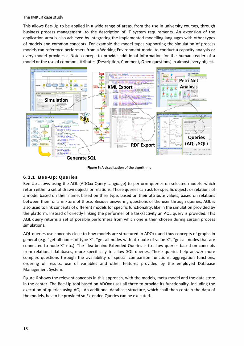
This allows Bee‐Up to be applied in a wide range of areas, from the use in university courses, through
business process management, to the description of IT system requirements. An extension of the
application area is also achieved by integrating the implemented modelling languages with other types
of models and common concepts. For example the model types supporting the simulation of process
models can reference performers from a Working Environment model to conduct a capacity analysis or
every model provides a Note concept to provide additional information for the human reader of a
model or the use of common attributes (Description, Comment, Open questions) in almost every object.
Figure 5: A visualization of the algorithms
6.3.1 Bee-Up: Queries Bee‐Up allows using the AQL (ADOxx Query Language) to perform queries on selected models, which
return either a set of drawn objects or relations. Those queries can ask for specific objects or relations of
a model based on their name, based on their type, based on their attribute values, based on relations
between them or a mixture of those. Besides answering questions of the user through queries, AQL is
also used to link concepts of different models for specific functionality, like in the simulation provided by
the platform. Instead of directly linking the performer of a task/activity an AQL query is provided. This
AQL query returns a set of possible performers from which one is then chosen during certain process
simulations.
AQL queries use concepts close to how models are structured in ADOxx and thus concepts of graphs in
general (e.g. “get all nodes of type X”, “get all nodes with attribute of value X”, “get all nodes that are
connected to node X” etc.). The idea behind Extended Queries is to allow queries based on concepts
from relational databases, more specifically to allow SQL queries. Those queries help answer more
complex questions through the availability of special comparison functions, aggregation functions,
ordering of results, use of variables and other features provided by the employed Database
Management System.
Figure 6 shows the relevant concepts in this approach, with the models, meta‐model and the data store
in the center. The Bee‐Up tool based on ADOxx uses all three to provide its functionality, including the
execution of queries using AQL. An additional database structure, which shall then contain the data of
the models, has to be provided so Extended Queries can be executed.

The IMKER case study
19
Figure 6: Bee‐Up Tool, AQL and Extended Queries
Following is a description of how the database structure for Extended Queries can be derived for the
BPMN modelling language with examples how it can be applied. This can be used as a basis for the other
modelling languages of Bee‐Up to derive their database structure.
Business Process Model and Notation
Examples for meaningful extended queries performed on BPMN models would be:
All decisions that split the path – in the context of IMKER this query could allow determining all
the decisions a beekeeper has to make.
All communication between participants of the process including direction and exchanged
messages (if available) – in the context of IMKER this query would indicate what information is
exchanged between whom in a process depicting the processing of an order.
The meta‐model provided in the Appendix I (Bee‐Up Handbook) section 5.1 together with the Bee‐Up
tool implementation can be used to derive a relational data structure for BPMN. The Bee‐Up tool is used
to determine details which are not covered by the provided meta‐model, like specific attributes
available. In general a relation with a primary key, foreign keys and other attributes will be described for
the relevant elements, namely the classes and the relations between classes (called relation classes in
this text to distinguish from the relational data structure). An approach similar to weak entities is used
to depict the class hierarchy to properly allow the use of foreign keys for relation classes. Certain
relations will be added to further provide type semantics and common attributes, like __Activity__
between __D‐construct__ and the relation depicting a BPMN Task.
The here presented relational data structure will not cover the entire BPMN Modelling Language,
instead focusing on providing the tables necessary to cover at least some cases. Some of the here
omitted classes and relation classes are: Group, Text Annotation, Association, Data Object, Conversation
and Data Association. Primary keys are indicated by bold and underlined text. Foreign keys are identified
by italic and underlined text. The relational data structure is split into three categories:

The IMKER case study
20
General abstract tables
This category describes general tables which can be used also by other modelling languages besides
BPMN (e.g. EPC, UML etc.). Abstract is meant here in the sense that for each of their rows there should
also be corresponding rows in other tables to simulate the class hierarchy. Those are used to a) provide
proper tables for foreign keys of certain relations and b) add overarching semantic to the elements (e.g.
BPMN Task, EPC Function and UML Activity as “sub‐types” of __Activity__).
__D‐construct__ (ID, name, modelID) – General table that represents any object in the model that is not a relation. Names have to be unique and not null. modelID is a foreign key referencing the ID of a specific model where the object is used. Almost anything that isn’t an instance of relation class or a model can be considered a “Weak entity” of __D‐construct__.
__D_container__ (ID) – Denotes objects that can contain other objects. ID is also a foreign key from __D‐construct__.
__Activity__ (ID, time, cost) – A general table for representing activities of any type. ID is a foreign key from __D‐construct__.
__Split_Merge__ (ID, type) – A general type for representing objects that can split or merge the path of a process. The type should denote how the split/merge should be interpreted (i.e. XOR: follow only one path, OR: follow several paths, AND: follow all paths). ID is a foreign key from __D‐construct__.
__Subgraph__ (ID, refModelID) – A general table for representing anything that can be further detailed by a model. ID is a foreign key from __D‐construct__ and refModelID is a foreign key from Model, indicating in which model the details are provided.
__Start__ (ID) – A general table for representing anything that starts a process. ID is a foreign key from __D‐construct__.
__End__ (ID) – A general table for representing anything that ends a process. ID is a foreign key from __D‐construct__.
General tables
This category describes general tables which make sense to be used also by other modelling languages
besides BPMN (e.g. EPC, ER etc.).
Model (ID, name, type) – Depicts a specific model in which objects are present.
Is_inside (sourceID, targetID) – Depicts which elements are in which container. sourceID is a foreign key from __D‐construct__ and targetID is a foreign key from __D_container__.
Subsequent (sourceID, targetID, denomination, probability) – Depicts the relations between the preceding and the following object in the process. The denomination can be used to denote conditions. Both sourceID and targetID are foreign keys from __D‐construct__.
Note (ID, content) – Depicts a note that can be attached to any object. ID is a foreign key from __D‐construct__.
has_Note (sourceID, targetID) – links an object to a note about it. sourceID is a foreign key from __D‐construct__ and targetID is a foreign key from Note.
Note: instances of relation classes belong to the model where their source and target are located.
BPMN specific tables
This category describes tables that are specific for BPMN models.
Message (ID, description, objectType) – Depicts a specific message that can be exchanged between two participants. The objectType indicates if it represents a physical message or just information. ID is also a foreign key from __D‐construct__.
Message_Flow (sourceID, targetID, denomination) – Depicts the flow of messages between objects in a specific direction. Both sourceID and targetID are foreign keys from __D‐construct__.
Pool (ID, processType, description) – Depicts a pool in the process (a Participant). ID is also a foreign key from __D_container__.
Lane (ID, description) – Depicts a lane that further divides a pool. ID is a foreign key from __D_container__.

The IMKER case study
21
Task (ID, type, loopType, description) – Depicts a specific task that is performed. Type identifies what sub‐type of task this is according to BPMN (service, send, receive etc.). loopType identifies what type of loop is used (e.g. NULL = no loop, 0 = standard loop, 1 = multi‐instance loop). ID is a foreign key from __Activity__.
Sub_process (ID, loopType, description) – Depicts a Task that is further described by another process model. loopType identifies what type of loop is used (e.g. NULL = no loop, 0 = standard loop, 1 = multi‐instance loop). ID is a foreign key from __Subgraph__.
Exclusive_Gateway (ID, description) – Depicts a point in the process (e.g. a decision) that either selects one following path or continues if at least one incoming path has been triggered (or both merge and split at once). ID is a foreign key from __Split_Merge__ and the type should always be XOR.
Non_exclusive_Gateway (ID, description) – Depicts a point in the process (e.g. a decision) that either splits into or merges from several or all paths. ID is a foreign key from __Split_Merge__ and the type should either be OR or AND.
Start_Event (ID, trigger, description) – Depicts the start of the process and what triggers it. ID is a foreign key from __Start__.
Intermediate_Event (ID, attachedTo, isCatching, isInterrupting, trigger, description) – Depicts an intermediate event according to BPMN. isCatching states if the task catches or throws the event, while isInterrupting is used only for events which are attached to a task (whether they interrupt the task or not). The trigger describes which trigger the event catches/throws. ID is a foreign key from __D‐construct__ and attachedTo is a foreign key from __D‐construct__ indicating if the intermediate event is attached to a boundary of a task or sub‐process.
End_Event (ID, trigger, description) – Depicts the end of the process and what it triggers. ID is a
foreign key from __End__.
A part of this relational data structure with some abstract examples is visualized in the following picture,
where the columns containing the primary key are in bold and underlined and foreign keys are italic and
underlined and are visualized through the arrows:

The IMKER case study
22
Based on this structure the question “Which decisions have to be made in the process?” can be
answered using an SQL query (for SQL Server 2012):
SELECT dc.id, dc.name FROM [Subsequent] AS subs INNER JOIN [__D‐construct__] AS dc ON dc.id=subs.sourceID INNER JOIN [__Split_Merge__] AS sm ON sm.ID=dc.ID AND
(sm.type='XOR' OR sm.type='OR') GROUP BY dc.id, dc.name HAVING COUNT(subs.sourceID)>1;
This query looks for all decisions in the __Split_Merge__ table that have an ‘XOR’/’OR’ type and only
selects the ones that have more than 1 outgoing subsequent relation.
Event‐driven Process Chains
Examples for meaningful extended queries performed on EPC models would be:
All Information objects used as input and where they are used, ordered by how often the
Information object is used in total – in the context of IMKER when using models that describe
the behavior of bees this could help analyze information exchange between bees and with their
environment, focusing on the ones exchanged most often.
All functions that have more than one responsible assigned – in the context of IMKER when
implementing an ERP system this query would indicate tasks which apply the four‐eye‐principle.
All documents that have to be signed by multiple people – an extension of the previous query
focusing on signing of documents instead of tasks.
The meta‐model provided in the Appendix I (Bee‐Up Handbook) section 5.2 together with the Bee‐Up
tool implementation can be used to develop the data structure for extended queries in EPC, similar to
how the extended queries for BPMN have been developed in the previous section.
Entity‐Relationship
Examples for meaningful extended queries performed on ER models would be:
All “ER Relations” that use more than one cardinality >1 – in the context of IMKER this query
would help creating the database by showing all “ER Relations” that require their own table.
All attributes and for which entities they should be available with the order based on the names
of the entity, resolving special cases like weak entities – in the context of IMKER this query
would help to see all the data considered relevant for each entity of the data model.
The meta‐model provided in the Appendix I (Bee‐Up Handbook) section 5.3 together with the Bee‐Up
tool implementation can be used to develop the data structure for extended queries in ER, similar to
how the extended queries for BPMN have been developed in a previous section.
Unified Modeling Language
Examples for meaningful extended queries performed on UML models would be:
All components and the components they are linked to through interface requirement and
implementation – when using a deployment diagram to describe hive placement and available
nectar sources in the context of IMKER this query can help determine what types of honey each
hive will produce.
All activities/actions that are executed in a specific state diagram and because of which state
they are executed – in the context of IMKER this query would return the activities/actions which
have to be performed by the beekeeper depending on the state of a bee hive.
The meta‐model provided in the Appendix I (Bee‐Up Handbook) section 5.4 together with the Bee‐Up
tool implementation can be used to develop the data structure for extended queries in UML, similar to
how the extended queries for BPMN have been developed in a previous section.

The IMKER case study
23
Petri Nets
Examples for meaningful extended queries performed on PN models would be:
Determine how often a transition could fire if certain preceding places are ignored – for a
machine that extracts and bottles honey in the context of IMKER this query would check how
many bottles of honey could be produced (based on the current stock of bottles and caps) while
ignoring how much honey is actually available or alternatively if only honey is available then
how many bottles and caps would be needed to bottle it all.
Determine how often each transition would have to fire to enable a follow up transition (with
only one place in between) – in the context of IMKER and the machine extracting honey this
query could be used to analyze bottle necks of the machine.
The meta‐model provided in the Appendix I (Bee‐Up Handbook) section 5.5 together with the Bee‐Up
tool implementation can be used to develop the data structure for extended queries in PN, similar to
how the extended queries for BPMN have been developed in a previous section.
6.3.2 Bee-Up: RDF Export Bee‐Up contains a description of its meta‐model in RDF and provides functionality to export models in
RDF as well. This allows the models created in Bee‐Up to be used with concepts and technologies from
the Semantic Web, like Linked Data, SPARQL or the Web Ontology Language (OWL), allowing for
different utilizations of the model data. Examples would be linking with other resources from the
Semantic Web, executing rules to check consistency of models or inference new data, and perform
queries using SPARQL.
Figure 7 shows a quick overview for the exposure of models as RDF, with the models, meta‐model and
the data store in the center. The Bee‐Up tool already has the RDF description of the meta‐model and
provides functionality for transformation of model data to RDF as an RDF Export. Both the meta‐model
and model descriptions as RDF can then be used with Semantic Web technologies.
Figure 7: Bee‐Up, RDF and Transformation

The IMKER case study
24
The RDF descriptions use certain constructs aligned with RDFS to properly describe the meta‐model and
models and the functionality is based on a prototype developed in the ComVantage project (see
http://www.comvantage.eu/, accessed 28.02.2017). The following table5 describes some of those
general constructs:
Specific RDF constructs
Some general constructs to be used as types. The cv: prefix stands for “http://www.comvantage.eu/mm#”
Construct Description
cv:m_Model A class containing models, meaning that a resource of this type represents a model. For example EPC Model is a subclass of this.
cv:o_Modelling_object A class containing elements used in models. For example the class Activity is a subclass of this class.
cv:r_Modelling_relation_a A class containing relations which have properties (attributes). The resources also use cv:from and cv:to to indicate the source and target of the relation. For example the relation Subsequent is a subclass of this class.
cv:r_modelling_relation_na A class of properties containing relations without properties (attributes). For example the inter‐model reference Responsible of a Task is an instance of this class.
cv:a_attribute A class of properties containing concept properties (attributes). For example the attribute Task type of a Task is an instance of this class.
cv:described_in A property stating that additional information about the subject (e.g. element, relation) can be found in a specific graph.
cv:from A property providing the source of a relation with properties (i.e. of cv:Modelling_relation_a type). The subject is the relation and the object is the source.
cv:to A property providing the target of a relation with properties (i.e. of cv:Modelling_relation_a type). The subject is the relation and the object is the target.
Table 1: Specific constructs for RDF export
Together with those constructs certain rules are used to export the models as RDF descriptions. The
following table5 describes some of those rules:
Model level
Note: “corresponding X” should be understood in context to the Metamodel level. For example when an instance of type “Activity” is transformed, then “the corresponding Object type class” means the concept created for the “Activity” object class (e.g. mm:o_Activity).
Modelling Concept Linked Data mapping
Any Model is … Instance of the corresponding Model type class.
An RDF‐Graph (called model graph).
Any Object is … Instance of the corresponding Object type class in every model graph where it is used.
5 Adapted from ComVantage Deliverable 3.1.2 – Specification of Modelling Method Including Conceptualisation Outline.

The IMKER case study
25
Any Relation with attributes is …
Instance of the corresponding Relation type class in every model graph where it is used.
It also has two properties indicating the source and target using cv:from and cv:to.
Any Relation without attributes is …
A triple where the subject is the source element and the object is the target element. The predicate should use the corresponding Relation type property. If the two elements are in different models then the statement should also be in both model graphs. The cv:described_in property should be used to state in both graphs where the other element can be found.
Any (not table) Attribute value is …
The object of a triple where the subject is the element and the predicate is the corresponding Attribute property.
Table 2: Some of the rules employed in the RDF export
The RDF descriptions can then be used for example with an RDF store like rdf4j to execute SPARQL
queries. The following SPARQL query answers a question that has also been asked in section 6.3.1,
“Which decisions have to be made in the process?” for BPMN processes:
PREFIX rdfs: <http://www.w3.org/2000/01/rdf‐schema#> PREFIX cv: <http://www.comvantage.eu/mm#> PREFIX mm: <http://austria.omilab.org/psm/content/bee‐up/1_2#> PREFIX : <http://austria.omilab.org/psm/content/beeup/IMKER#> SELECT (?decision AS ?id) (?label AS ?name) WHERE { # This union merges the two different possible types of gateways denoting a decision. { # This pattern fits any OR Gateway that splits the paths. ?decision a mm:o_Non‐exclusive_Gateway_BPMN . ?decision mm:a_Gateway_type "Inclusive" } union { # This pattern fits any XOR Gateway. ?decision a mm:o_Exclusive_Gateway_BPMN } # This pattern matches subsequent relations which originate in one of the decisions. ?subsequent a mm:r_Subsequent . ?subsequent cv:from ?decision . ?decision rdfs:label ?label # This pattern retrieves the label of the decision. } GROUP BY ?decision ?label # Filters out any decision that has 1 or less subsequent paths. HAVING (count(?subsequent)>1)
This query binds anything that denotes a BPMN decision and its relevant data and only selects the ones
that have more than 1 outgoing subsequent relation.

The IMKER case study
26
6.3.3 Bee-Up: Generate SQL Besides being able to model Entity‐Relationship models, it is also possible to use them in Bee‐Up to
generate the SQL statements for creating tables. Used together with a database, it creates the table
structure described by the ER model. Figure 8 shows a quick overview for the generation of the SQL
statements, with the models, meta‐model and the data store in the center.
Figure 8: Bee‐Up and SQL generation
The functionality covers many different cases that can be described in an ER model and tries to achieve
a good structure for the tables based on that description of the data structure. Some of those are the
handling of relations based on the specified cardinalities, the resolution of weak entities and their
dependencies and the inheritance between entities.
The following ER model depicts for example part of the database structure for the Business Process
Model and Notation from section 6.3.1. It should be noted that not all information of the model is
visible in the picture, like the SQL datatypes of attributes, or the role names used for foreign keys to
prevent name‐clashes.
The IMKER case study
27
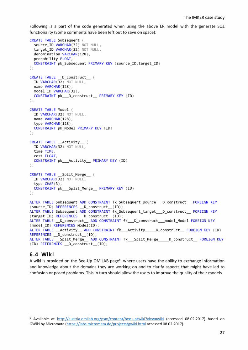
Following is a part of the code generated when using the above ER model with the generate SQL
functionality (Some comments have been left out to save on space):
CREATE TABLE Subsequent ( source_ID VARCHAR(32) NOT NULL, target_ID VARCHAR(32) NOT NULL, denomination VARCHAR(128), probability FLOAT, CONSTRAINT pk_Subsequent PRIMARY KEY (source_ID,target_ID) ); CREATE TABLE __D_construct__ ( ID VARCHAR(32) NOT NULL, name VARCHAR(128), model_ID VARCHAR(32), CONSTRAINT pk___D_construct__ PRIMARY KEY (ID) ); CREATE TABLE Model ( ID VARCHAR(32) NOT NULL, name VARCHAR(128), type VARCHAR(128), CONSTRAINT pk_Model PRIMARY KEY (ID) ); CREATE TABLE __Activity__ ( ID VARCHAR(32) NOT NULL, time TIME, cost FLOAT, CONSTRAINT pk___Activity__ PRIMARY KEY (ID) ); CREATE TABLE __Split_Merge__ ( ID VARCHAR(32) NOT NULL, type CHAR(3), CONSTRAINT pk___Split_Merge__ PRIMARY KEY (ID) ); ALTER TABLE Subsequent ADD CONSTRAINT fk_Subsequent_source___D_construct__ FOREIGN KEY (source_ID) REFERENCES __D_construct__(ID); ALTER TABLE Subsequent ADD CONSTRAINT fk_Subsequent_target___D_construct__ FOREIGN KEY (target_ID) REFERENCES __D_construct__(ID); ALTER TABLE __D_construct__ ADD CONSTRAINT fk___D_construct___model_Model FOREIGN KEY (model_ID) REFERENCES Model(ID); ALTER TABLE __Activity__ ADD CONSTRAINT fk___Activity_____D_construct__ FOREIGN KEY (ID) REFERENCES __D_construct__(ID); ALTER TABLE __Split_Merge__ ADD CONSTRAINT fk___Split_Merge_____D_construct__ FOREIGN KEY (ID) REFERENCES __D_construct__(ID);
6.4 Wiki A wiki is provided on the Bee‐Up OMiLAB page6, where users have the ability to exchange information
and knowledge about the domains they are working on and to clarify aspects that might have led to
confusion or posed problems. This in turn should allow the users to improve the quality of their models.
6 Available at http://austria.omilab.org/psm/content/bee‐up/wiki?view=wiki (accessed 08.02.2017) based on GWiki by Micromata (https://labs.micromata.de/projects/gwiki.html accessed 08.02.2017).

The IMKER case study
28
Appendix I: Bee-Up Handbook www. .org
1. General information This Handbook is written for Bee‐Up version 1.3 based on the ADOxx 1.57 platform. The Bee‐Up tool enables modelling according to the following languages and techniques:
Business Process Model and Notation 2.0 (BPMN),
Event‐driven Process Chains (EPC) with extensions,
Entity‐Relationship (ER), and
Unified Modeling Language 2.0 (UML)
Petri Nets (PN).
If you should encounter problems, have questions or feature requests which are not covered yet, you can also contact us directly:
Patrik Burzynski ( [email protected] )
Prof. Dimitris Karagiannis
2. Installation The Bee‐Up tool requires a Windows operating system (XP, Vista, 7, 8, 8.1 or 10). To install it on a
different OS please use virtualization software (e.g. VirtualBox or VMware)8 and a windows license9.
To install the Bee‐Up tool follow these steps: 1. Download the ZIP‐File containing the installation package from OMiLAB. 2. Extract the contents to a folder. 3. Run the setup.exe from the extracted folder.
The setup first informs about prerequisites that will be installed automatically. This includes required
frameworks (e.g. .NET) and the creation of a SQL Server instance where necessary. Once those tasks are
finished a wizard will guide you through the remainder of the installation.
Note that if the setup automatically created a SQL Server instance, it is called ADOXX15EN and has set
the initial ‘sa’ password to ‘12+*ADOxx*+34’ (without the ‘ ’ ). If you want to use an already available
SQL Server database instance, it has to use “Mixed mode” for authentication. Should you no longer
remember the ‘sa’ password: help on how to reset the ‘sa’ password can be found at the ADOxx.org
community.
By default Bee‐Up 1.3 will create and use the database with the name ‘beeup13’ (without the ‘ ’ ), unless
a different one has been specified during the installation (for example when ‘beeup13’ is already used
by something else).
Some additional functionality provided by Bee‐Up (beyond simple modelling, e.g. RDF Export) also
requires a functioning Java 1.8 installation. A download link and installation instructions can be found at
https://java.com.
7 http://www.adoxx.org/ 8 Obtainable from https://www.virtualbox.org/ or http://www.vmware.com/ respectively 9 As a student of computer science on the University of Vienna you can get access to different versions of windows at http://cs.univie.ac.at/students/info/software/msdn/

The IMKER case study
29
2.1 Things to watch out for before/during/after installation
2.1.1 Before the installation 1. Language for non‐Unicode programs: Make sure that the “Language for non‐Unicode programs” of
the operating system is set properly. This setting can be found in the “Control Panel” under “Region and Language” in the “Administrative” tab, as shown in the picture below. Languages like English and German are known to work for Bee‐Up among others. Similar languages should most likely pose no problem. Languages using characters which are very different from English (like Greek, Persian or Chinese) can however pose a problem. If an error saying “The selected database does not exist or has not been catalogued yet.” is encountered during the installation or an error like “Database … does not exist!” pops up when starting the tool after the installation, then it’s most likely due to this setting. In this case please uninstall the tool and the SQL Server instance “ADOXX15EN”, change the setting and install Bee‐Up again. Alternative: It might also be possible to work with a different “Language for non‐Unicode
programs”, which however requires a manual installation of the SQL Server instance. A detailed
step‐by‐step guide can be found at the ADOxx homepage (Download Windows Installation Guide
Installation of different collation database (Non‐Latin Database Instance)). Please note that this
has not been tested by our developers for Bee‐Up.
2.1.2 During the installation 1. Installation of SQL Server instance fails: It is possible that the installation of the SQL Server
instance fails, typically with an error message like “Failed to install Microsoft SQL Server (instance ADOXX15EN). Please check for errors and try again.”, in which case the tool will not be properly installed. One of the reasons is that the SQL Server installer performs a check and the system doesn’t meet the necessary requirements. One of the requirements is that a system restart is

The IMKER case study
30
possible. Sometimes a different application can block the system restart, leading to the problem. So one possible solution is to close all other applications, restart the computer and then perform the installation. Another approach is to manually install the SQL Server instance beforehand. Detailed descriptions for this can be found in the “dbinfo” folder (the PDF‐files with “install” like “BOC‐Product_sqlserver_2008_express_install_en.pdf” are relevant, not “createdb”) and the folder “SQLExpress” folder contains an installation file for the SQL Server. Please note that the “Instance ID” MUST be “ADOXX15EN”!
2. Installation asks for standard administrator “sa” password: Sometimes during the installation a popup can ask for the database standard administrator password (see picture below). Some users reported, that after aborting the installation and restarting the computer the popup no longer appeared. Alternatively, if the SQL Server instance has been created automatically by the installation, then it has set the initial ‘sa’ password to ‘12+*ADOxx*+34’ (without the ‘ ’ ). Help on how to reset the ‘sa’ password can be found at the ADOxx.org community (in the FAQ: “SA Password during ADOxx Installation”).
2.1.3 After the installation 1. Database connection failed: Bee‐Up uses a database to store all the information in the background.
Therefore during the installation an SQL Server instance is automatically created. However, it can happen when starting the tool that an error is encountered with the message “ADOxx could not connect to the database …! Please try again.” This can happen when the database service is not running. Please make sure that the proper SQL Server service is running (“SQL Server (ADOXX15EN)” in the services panel of Windows) and try starting Bee‐Up again.
2. Loosing connection to database while tool is running: On some systems (especially when using Windows 10) it can happen that the connection from Bee‐Up to the database is lost, usually with an error message like “Due to a database exception the connection has been closed …” This often happens due to a longer inactivity which can lead to a connection time out. Unfortunately a consequence of this is a loss of all the changes that have been made since the last save. It can however often be prevented from happening by opening the “SQL Server Configuration Manager” tool, selecting “Protocols for ADOXX15EN and disabling both “Named Pipes” and “TCP/IP” as shown in the picture below.

The IMKER case study
31
2.1.4 Uninstallation Yes, it is also possible to uninstall Bee‐Up if so wished or necessary. Please note that this will of course
also delete all the created models that are stored in the database. Therefore it is advised to first back up
everything from Bee‐Up that should be saved using the Export functionality (see section “Exporting and
importing models”).
To completely uninstall Bee‐Up, two things should be performed:
1. Uninstall the Bee‐Up tool – This can simply be achieved through the systems control panel. 2. Uninstall the Microsoft SQL Server – Here the SQL Server instance used by Bee‐Up (“ADOXX15EN”)
should be uninstalled, again using the control panel. IMPORTANT: This will also remove all the data stored in all the databases of the SQL Server instance. If other ADOxx based tools have been installed and use the “ADOXX15EN” instance, or other relevant data has been put there, then it is not advised to uninstall the SQL Server instance, since it could break the other applications!

The IMKER case study
32
3. Modelling with the Bee-Up tool
3.1 Tool overview When first starting the Bee‐Up tool you see a screen similar to the following one (without the numbers):
At the top is the menu bar with different menu items for direct access to some of the platforms
functionality. The numbered elements of the above picture are:
1. The Toolbar with icons as shortcuts for different functions. On the left side of the toolbar is the component selection:
This changes which menus, menu items and toolbar icons are available. The two important components are “Modelling” (left most icon) and “Import/Export” (right most icon). The current section of this document focuses on the “Modelling” component, while the next will describe some functionalities of the “Import/Export” component.
2. The Start Page is visible, showing recently opened models. The Start Page can be accessed
through the house icon in the Toolbar. Once a model is opened it will be shown instead of the Start Page. This area is then referred to as the Modelling area.
3. The Modelling window shows the modelling objects and relations available for the currently opened model (in the figure above none, because no model is open).
4. The Explorer window shows all folders (called model groups) and the models, stored in a model group. Initially, model groups for all exercise sheets are preconfigured, accompanied by a testing model group.
5. The Navigator window shows an overview of the currently opened model.
1.
5.
2.
4.
3.

The IMKER case study
33
3.2 Creating a new model In order to create a new model select the menu item “Model New…” while in the “Modelling”
component ( left most icon in the Toolbar).
This will open the dialog shown below (without the numbers):
In this dialog first select the appropriate filter for the model types (e.g. Entity‐Relationship for ER‐
models), either by using the graphic on the left side (1.) or the dropdown‐list in the middle (2.).
Afterwards, select the desired model type from the list in the middle (3.). Then enter a name
(mandatory) and a version (optional) on the right side (4.). Finally, select to which exercise sheet (model
group) the model should be assigned10 (5.) and click on “Create”. Please use the appropriate model
group for your case (i.e. if it is a solution for a specific assignment, use the corresponding model group).
This will create an empty model of the selected modelling technique, store it in the selected model
group and open it, ready to be edited.
10 Or select „Testing“ (model group) when you are creating a model for testing purposes (e.g. to see how everything works, play around, explore the tool etc.).
1. 2.
3.
4.
5.

The IMKER case study
34
The picture above shows an example for a newly created and opened Entity‐Relationship model. The
Modelling area (2.) now shows the empty Drawing area (a white canvas to drag & drop objects and
relations) instead of the Start Page. The Modelling window (3.) shows the available types of objects and
relations that can be used for ER modelling, e.g., Entity, Relationship, Attribute. The created model can
also be seen in the Explorer window (4.) under the selected exercise sheet (model group). The
Navigator window (4.) shows the complete model, enabling direct navigation and zooming, as well as
the portion that is currently shown in the Modelling area.
3.3 Editing the model To edit a model it hast to be opened in the Bee‐Up tool. The easiest way to open a model is to double
click on its name in the Explorer window. New objects can be added to the model by selecting the type
of object that should be added in the Modelling window and then clicking in the Modelling area where
the object should be placed. If necessary the Drawing area will be extended automatically. After adding
a few objects, the Modelling area could look like this:
2.
4.
3.
5.

The IMKER case study
35
In order to connect objects with relations, first select the relation type from the Modelling window.
Then click in the Modelling area on the object that is the source (“starting point”) of the relation and
then on the object that is the target (“ending point”) of the relation. Certain types of relations can only
be used between specific types of objects (e.g. “has Attribute” always has to target an “Attribute”). The
previous example with some relations could look like this:
All objects can be moved in the Modelling area by selecting them and moving them accordingly. Some
objects can also be resized, which works similar to resizing windows in the operating system (drag the
side/corner when it is selected). For both the “Edit” function has to be selected in the Modelling
window (looks like the default mouse cursor). After creating objects and relations you can quickly switch
back to “Edit” by pressing the right mouse button. It is also possible to move/resize several objects at
once by selecting them first (draw selection box around them, SHIFT+Click, CTRL+Click) and then
performing the move or resizing. The difference between SHIFT+Click and CTRL+Click is that using SHIFT
will select the object and all of the objects it contains if it is a container (like a “Package”, “State”,
“Combined Fragment”, “Lifeline” etc.) while using CTRL will not. This is useful when a container should
be moved with all of its contents at once.
3.4 Adding edges to relations It is also possible to add bend points to relations. Those force the relation to be drawn through that point and can increase readability of the created models. The following image shows a relation with six bend points (small white rectangles):
Bend points can be added either during the creation of the relation, or afterwards. To add bend points
during the creation first click on the source, then click on the desired points in the Modelling area where
a bend point (i.e. an edge) should be drawn, and finally click on the target object. To add them after the
relation has been created, select the relation first and then click and drag a point of the relation (that
isn’t already a bend point) to the desired place on the Modelling area.
The source or the target of a relation can also be changed by selecting the relation and then clicking the
yellow circle at the beginning or the end and dragging it to the new object that should be the source or
target. The green diamond that is visible when a relation is selected can be used in many cases to move
the text that is visualized next to it (e.g. the cardinality of the “Links” relation; ‘m’ in the figure above).

The IMKER case study
36
3.5 Editing attributes All objects, models and relations can have editable attributes, which can also influence their
visualization in the Modelling area (e.g. weak entities have a double outline instead of a single one).
Those attributes can be accessed by double‐clicking on the object or relation (or selecting it and then
pressing Enter). This opens up the ADOxx Notebook, which contains the attributes that can be edited.
To access the attributes of a model it has to be opened first and then select the menu item “Model
Model attributes” or press ALT+Enter. The following picture shows an example of a Notebook:
The attributes take up the largest portion of the Notebook and are categorized in different tabs,
available on the right side of the Notebook. Depending on the attribute type different editors for the
attribute value are available (e.g. single‐line text field for the Name, multi‐line text area for the
Description, checkbox for the Weak entity etc.). For some attributes an alternative editor can be
accessed through the button. Also additional information is available for most of the attributes and
can be accessed by clicking on the icon. A similar icon can be found at the top right (underneath the X
for closing the window), which provides information about the type of the object. The two
buttons at the lower right are an alternative to switching between the different categories. They are also
used to switch between pages of one category, in the case that more attributes are available than can
be shown in the Notebook window.
There are two special types of attributes that have to be described in more detail: 1. Inter‐model references – they allow to link (reference) to one or several other objects or models
and have three special icons: . The first one (+) allows to add new references, while the second one (X) removes the selected references. The third one () is like a hyperlink that jumps to the referenced object. Often when the attribute value is visualized it also works as a hyperlink in the Modelling area.
2. Tables – they allow to store more complex attribute values in a structured way. They also have
two special icons: . The first one (+) is used to add a new row at the end and the second one (X) removes the selected rows. Note that in order to select rows the number on the left side has to be clicked. The context menu also provides several options to handle rows in a table (e.g. insert row, move row, etc.)

The IMKER case study
37
It is also possible to edit some of the attribute values that are visualized in the Modelling area without
using the Notebook. For this simply select the object and then click on the visualized attribute value
(e.g. the name: “Entity (ER)‐317265”). Note that this prevents opening the Notebook although the
attribute is being edited.
4. Exporting models The tool also provides functionality to export the created models in different formats. Some of those will
be described here. Most of them are available in the “Import/Export” component ( )
4.1 Creating a graphic from a model It is possible to create a graphic of the currently opened model and store it in a file using the provided
“Generate graphics” functionality ( icon in the Toolbar available when using the “Modelling”
component). This opens a dialog showing the region of the model for which the graphic will be created
as well as options to scale the created picture and to either save it in a file (with different formats
available) or copy it to the clipboard. Clicking on the “Generate” button will finish the process.
The region can be set beforehand by holding down the ALT key and click‐and‐dragging a box in the
Modelling area with the mouse. This will create a teal rectangle (that can also be resized) showing what
region will be used for generating the graphic. The following picture shows the dialog for the previous
example model, where a fitting region has been set:
4.2 Exporting the exercise It is also possible to export an entire exercise at once. This can be achieved by using the menu item
“Model Export Exercises” (or using the icon in the Toolbar). This will show a dialog where the
model group containing all of the solutions for the exercise can be selected. Afterwards a new dialog
asks for a folder where the results should be stored. Once it is finished a message will inform you about
it.
This functionality exports all of the models contained in the selected model group or one of its
descendent sub‐groups in ADL format and also creates individual graphic files for all of the models. The
creation of the graphic can sometimes fail when the name and/or version contain a character that is not
supported by the operating system as a filename11. IMPORTANT: It also removes empty space from the
right and the bottom in the drawing area (in the Modelling area) AND saves the model before
generating the graphic.
11 Common ones like „:“, „/“, „*“ etc. are replaced by a „‐" for the file name.

The IMKER case study
38
4.3 Exporting and importing models One or several models as well as model groups can be exported to/imported from either the ADL format
(proprietary) or XML format by using the according menu items in the “Model” menu (e.g. “Model
XML export (default)…”).
For the export a simple dialog is show where the models and/or model groups are selected at the top.
The middle of the dialog contains some checkboxes to control what should be exported (e.g. “Including
models”, “Including model groups” etc.) and at the bottom the file is specified where the models/model
groups should be exported to. The export is started by clicking on the “Export” button and at the end a
success or error message is shown.
For the import there are several tabs available. In the “File selection” tab the file containing the
models/model groups is selected. The “Model options” tab provides some choices on how to deal with
collisions (e.g. what to do when two models have the same name). The last tab “Log file” allows logging
the process in a file. After everything is selected click on the “OK” button. This will prepare the data
from the previously selected file and open another dialog. Here the left side shows which models and/or
model groups have been found in the file and you can select which of those should be imported. On the
right side select into which model group the contents should be imported and click on the “Import”
button. At the end a success or error message is shown.
4.4 Exporting models as RDF A new function in Version 1.1 adds the possibility to export one or several models in RDF Format. This
can be simply accessed through the menu item “Model RDF Export”. The first dialog asks which
models should be exported. Here either directly the models or entire model groups can be selected.
Afterwards a file selection dialog will ask where the RDF data should be stored and allows a choice of
different formats (.trig is recommended). A third dialog will ask for a base URI to be used in the
identifiers as a prefix. Here it is recommended to use a valid URL without the fragment (for example
http://www.omilab.org/example# or http://www.example.net/#). It is not necessary for the URL to be
actually used (i.e. the URL can return an error code like 404), just that the URL is valid. Once it is finished
a message will inform you about it.
With Version 1.2 additional attributes have been added to (almost) all elements and models to enhance
the RDF Export. These are found in the “RDF properties” tab of the Notebook. The “URI” attribute allows
specifying a specific URI to be used for the element/model instead of automatically generating a URI.
The “Additional Triples” table allows specifying additional triples (Subject, Predicate and Object) that will
be added to the graph, where one row represents one triple. If a cell is left empty in the “Additional
Triples” table, then it will be substituted with the URI of the element/model it is located in. Note that
the values provided in those attributes will be treated as is as a complete URI (ignoring prefixes etc.).
Therefore, it is necessary to enter the entire URI. Also with Version 1.2 the names of elements and
models are exported explicitly as rdfs:label statements.

The IMKER case study
39
5. Additional hints and information
5.1 Specific information for BPMN modelling The BPMN implementation provides concepts to describe processes, as well as for describing input,
output and execution of “Tasks”. Two different modes are available, which limit the available concepts.
By default the “BPMN 2.0” mode is selected, which contains the typical BPMN concepts. However, the
mode can be changed (through the menu “View Mode”) to “Simulation”. This mode further adds
concepts which are necessary to perform simulation of processes in the tool (e.g. converging gateways
as their own types). The following picture shows the two modes and which types of elements they use:
The majority of BPMN should be straight forward and some constraints are enforced by the tool (e.g.
“Start Events” cannot have any incoming “Subsequent” relations). However, due to certain platform
restrictions the Gateways (Exclusive, Inclusive, Parallel etc.) are handled a bit differently12. In the
standard BPMN mode the Exclusive Gateway is available as its own type (“Exclusive Gateway”), however
the Inclusive and Parallel Gateway are modelled through the “Non‐exclusive Gateway”. The type
(Inclusive, Parallel or Complex) is then set through the attribute “Gateway type” (in the Notebook)13.
Previously the Intermediate event was split into two different types: “Intermediate Event (boundary)”
and “Intermediate Event (sequence)”. Since Version 1.1 the two have been merged into one and are
distinguished through setting the “Attached to” Attribute. If the attribute has a value it will be
considered on the Boundary of the set “Task”. A new Mode has been added called “Deprecated”, which
allows the use of the two old Intermediate events in order to not destroy previously created models.
Those events can easily be transformed into the new “Intermediate Event” by right clicking on them and
selecting “Convert Intermediate Event (BPMN)”.
12 This is due to the way simulation is handled by the platform. 13 “Simulation” mode additionally has a “Non‐exclusive Gateway (converging)”, which is necessary for the simulation.

The IMKER case study
40
Certain types of objects can be converted into other types (e.g. “Exclusive Gateway” to “Non‐exclusive
Gateway”) by selecting them and then using “Conversion” in the context menu. An object will become
greyed out and cannot be selected, if it is converted to a type that is not available in the current mode.
To transform it back (or delete it or change it etc.), simply change the mode to one that makes use of
the type (e.g. “All modelling objects”). The picture below shows the available options for converting the
“Exclusive Gateway”:
The availability of some attributes (in the Notebook) is dependent on the values of others. This is to
prevent setting wrong values or changing irrelevant attributes. For example the available “Triggers” of a
“Start Event” depend on its “Type” to prevent wrong selections. Another example is the “Loop condition
(standard)” attribute of a “Task”, which is only available when the “Loop type” is set to “Standard”
(otherwise it is irrelevant).
The relation “Subsequent” has an attribute “Visualized values”, which controls which attribute values
are shown. Should the desired value not be shown on the drawing area (e.g. “Transition condition”)
then it might be because of the “Visualized values” attribute. “Subsequent” is also used in several
different model types (e.g. EPC, UML Activity Diagram). Therefore it also contains attributes used in
those model types. They are however grouped in their own categories (e.g. “UML properties”).
For many different types of objects (e.g. “Start Event”, “Exclusive Gateway” etc.) the visualization of the
name can be controlled through the attribute “Show name”. In some cases this is a simple choice if the
name should be displayed (e.g. “Start Event”). In other cases more options are available (e.g. “Exclusive
Gateway”).
Version 1.2 also added the option to further describe Service Tasks through Petri Nets or Flowcharts
using the “Automated service details” attribute. The attribute should reference the starting point in the
Petri Net or Flowchart.
The following picture provides some detailed information about the implementation of BPMN in Bee‐
Up. More specifically it shows an excerpt of how the BPMN meta‐model is implemented. Certain parts
are provided by the platform to allow specific functionality, like __D_event__ and Subsequent used for
process simulation. The “…” abstract class is used to represent complex generalization structures in the
meta‐model in a simplified manner.

The IMKER case study
41
5.2 Specific information for EPC modelling The EPC implementation provides the core concepts from Event‐driven Process Chains to describe
processes (“Event”, “Function”, logical operators), as well as some additional ones for describing input,
output and execution of “Functions”. Different modes can be selected, which limit the available
concepts. By default the “EPC” mode is selected, which contains “Events”, “Functions” and the basic
logical operators from EPC (also some additional “general” concepts). However, the mode can be
changed (through the menu “View Mode”) to “eEPC” or “Simulation”. “eEPC” (extended EPC)
additionally contains “Organizational units”, “Information objects” and relations for those new object
types. The relations for denoting inputs and outputs for “Functions” are implemented as separate types.
“Simulation” mode further adds concepts which are necessary to perform simulation of processes in the
tool (e.g. “Start Event” which explicitly denotes the start of the process). The following picture shows
the three modes and which types of elements they use:

The IMKER case study
42
The majority of EPC should be straight forward and some of the constraints of an EPC model are
enforced by the tool (e.g. between two “Functions” there has to be an “Event”). However, due to certain
platform restrictions the typical logical operators (XOR, OR, AND) are handled a bit differently14. In the
basic “EPC” and “eEPC” the XOR operator is available as its own type (“XOR operator”), however the
AND and OR operators are modelled through the “Parallel fork”. The type (AND or OR) is then set
through the attribute “Type” (in the Notebook)15. In “EPC” and “eEPC” mode the “Parallel fork” is used
both for splitting and merging paths.
The relation “Subsequent” has an attribute “Visualized values”, which controls which attribute values
are shown. Should the desired value not be shown on the drawing area (e.g. “Transition condition”)
then it might be because of the “Visualized values” attribute. “Subsequent” is also used in several
different model types (e.g. BPMN, UML Activity Diagram). Therefore it also contains attributes used in
those model types. They are however grouped in their own categories (e.g. “UML properties”).
Certain types of objects can be converted into other types (e.g. “Event” to “Start Event” or “End Event”,
“XOR operator” to “Parallel fork” etc.) by selecting them and then using “Conversion” in the context
menu. An object will become greyed out and cannot be selected, if it is converted to a type that is not
available in the current mode. To transform it back (or delete it or change it etc.), simply change the
mode to one that makes use of the type (e.g. “All modelling objects”). The picture below shows the
available options for converting the “XOR operator”:
Version 1.2 also added the option to further describe Functions through Petri Nets or Flowcharts using
the “Automation details” attribute. The attribute should reference the starting point in the Petri Net or
Flowchart.
The following picture provides some detailed information about the implementation of EPC in Bee‐Up.
More specifically it shows an excerpt of how the EPC meta‐model is implemented. Certain parts are
provided by the platform to allow specific functionality, like __D_event__ and Subsequent used for
process simulation. The “…” abstract class is used to represent complex generalization structures in the
meta‐model in a simplified manner.
14 This is due to the way simulation is handled by the platform. 15 “Simulation” mode additionally has a “Parallel merge”. This distinction between fork and merge is necessary for the simulation algorithm.
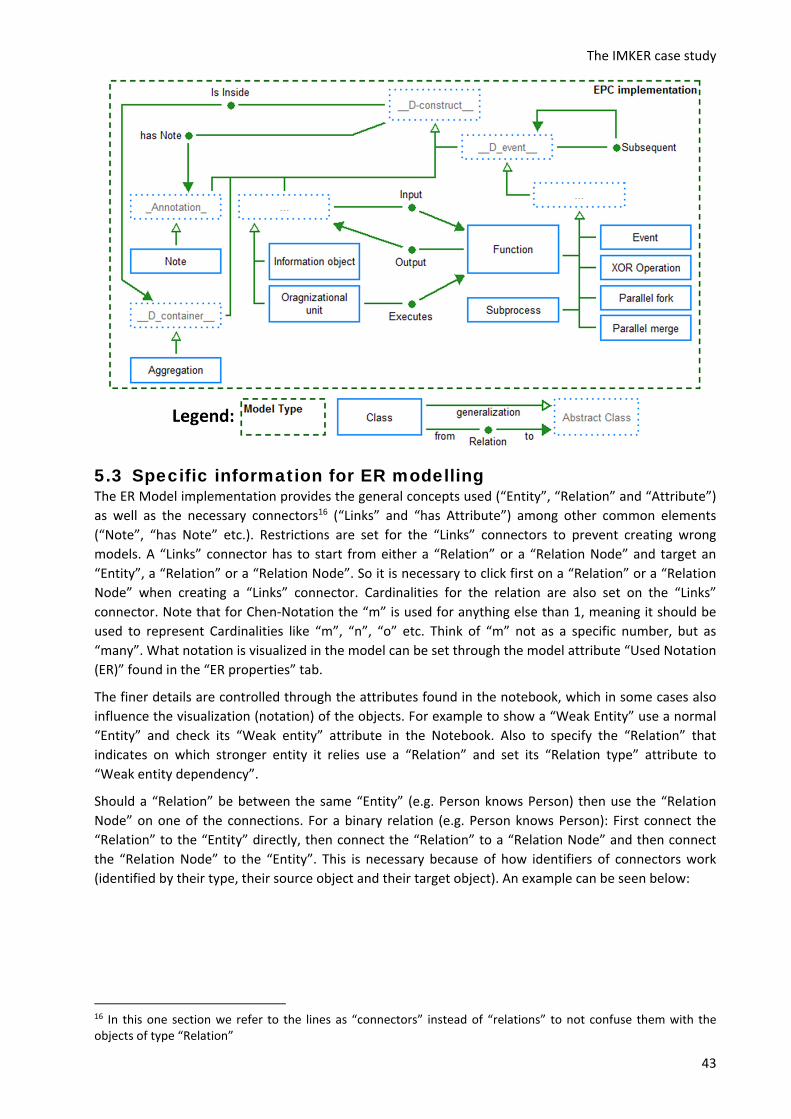
The IMKER case study
43
5.3 Specific information for ER modelling The ER Model implementation provides the general concepts used (“Entity”, “Relation” and “Attribute”)
as well as the necessary connectors16 (“Links” and “has Attribute”) among other common elements
(“Note”, “has Note” etc.). Restrictions are set for the “Links” connectors to prevent creating wrong
models. A “Links” connector has to start from either a “Relation” or a “Relation Node” and target an
“Entity”, a “Relation” or a “Relation Node”. So it is necessary to click first on a “Relation” or a “Relation
Node” when creating a “Links” connector. Cardinalities for the relation are also set on the “Links”
connector. Note that for Chen‐Notation the “m” is used for anything else than 1, meaning it should be
used to represent Cardinalities like “m”, “n”, “o” etc. Think of “m” not as a specific number, but as
“many”. What notation is visualized in the model can be set through the model attribute “Used Notation
(ER)” found in the “ER properties” tab.
The finer details are controlled through the attributes found in the notebook, which in some cases also
influence the visualization (notation) of the objects. For example to show a “Weak Entity” use a normal
“Entity” and check its “Weak entity” attribute in the Notebook. Also to specify the “Relation” that
indicates on which stronger entity it relies use a “Relation” and set its “Relation type” attribute to
“Weak entity dependency”.
Should a “Relation” be between the same “Entity” (e.g. Person knows Person) then use the “Relation
Node” on one of the connections. For a binary relation (e.g. Person knows Person): First connect the
“Relation” to the “Entity” directly, then connect the “Relation” to a “Relation Node” and then connect
the “Relation Node” to the “Entity”. This is necessary because of how identifiers of connectors work
(identified by their type, their source object and their target object). An example can be seen below:
16 In this one section we refer to the lines as “connectors” instead of “relations” to not confuse them with the objects of type “Relation”

The IMKER case study
44
Functionality for creating SQL statements from an ER Model is also provided. It can be accessed through
the “Model” menu of the “Import/Export” component. A description with the quirks and details can also
be found in the same menu. The functionality uses the currently active model and will ask for a file to
store the created SQL code in. If the selection of a file is cancelled it will instead show the SQL code in a
pop‐up window from where it can be copied to the clipboard. Version 1.2 added two SQL properties to
“Attribute”: 1) one for directly entering the data type of the attribute and 2) to specify auto‐increment
(only works for MySQL). Version 1.3 changed how to handle inheritance through “IS‐A” relations. Two
options are available as Model attribute “IS‐A Behaviour”: 1) the “old” style where the table is copied
and 2) [now default] which handles inheritance similar to Weak Entities.
The following picture provides some detailed information about the implementation of ER in Bee‐Up.
More specifically it shows an excerpt of how the ER meta‐model is implemented. Certain parts are
provided by the platform to allow specific functionality, like __D_container__ used to automatically
derive “Is Inside” relations.

The IMKER case study
45
5.4 Specific information for UML modelling UML and its implementation in the tool are big. Addressing all of the peculiarities would be difficult and
also a lot of text to read. Therefore, they are addressed in general and some examples are provided.
Notations17 are generally influenced by the attribute values that are specified for them (in the notebook):
Most of the attributes that deal only with the visualization are located in a category called “Presentation”. Examples for such attributes are “Color” (of the object background), “Representation” (of text) and “Presentation” (of class details).
The “Subsequent” relation and the “Activity edge” use the attribute “Visualized values” to control which attribute values should be shown (e.g. Denomination, Transition condition, Weighting etc.).
Relations often have an option on where the text should be shown, handled through a “Representation” attribute. In general “above/below” value should be used for parts of relations going horizontally and “left/right” value for parts of relations going vertically. As an example the “Association” used in “Class / Object Diagrams” can have text in three parts: at the start, at the middle and at the end. For the start and the end a different “Representation” value can be set. If for example the association class starts going from the object towards the right (horizontal) and then turns towards the bottom (vertical) then the “Representation start” should use “above/below”, the “Representation end” should use “left/right”. In most cases the middle part uses a notation that works well with both horizontally and vertically drawn relations.
UML Specific attributes (e.g. “IsAbstract”, “Visibility” etc.) are usually located in a category called “UML properties”. In some cases they are located in the “Description” category (e.g. the “Type” of a “Final Node”) for quicker access or have their own category (e.g. “Properties/Operations” of a “Class”). Some of them also influence the notation, like the “Final type” attribute of a “Final Node” in an “Activity Diagram” or the “Properties” entered in a “Class”.
Certain relations, like the “Message” from a “Sequence Diagram”, have their sub‐types controlled
mostly through the attributes. So the typical types like “synchronous call”, “asynchronous call” and
“reply” are handled through the “Message sort” attribute of the “Message” relation.
In order to draw several relations between the same two objects in the same direction (e.g. several
“Associations” between the same two “Classes”) the “Relation Node” has to be used. For every
additional relation beyond the first one it is necessary to create two relations: one has to go from the
source object to a “Relation Node” and the other from that “Relation Node” to the target object. This is
necessary because of how identifiers of relations work18. For example when there are the classes
“Employee” and “Department” and two associations “works for” and “manager of” between the two
classes. The “manager of” association can go directly from “Employee” to “Department”. However, the
“works for” association has to be split in two: one association going from “Employee” to a “Relation
Node” and another from the same “Relation Node” to the “Department”. The attributes should also be
split among those two relations accordingly (i.e. the multiplicity for the “Employee” side of “works for”
has to go to the first relation, the multiplicity for the “Department” side of “works for” has to be in the
second relation and the name can be in one of those). The example can be seen below:
17 The look of an object on screen or on paper. 18 A relation is identified by its type, its source object and its target object. Duplicate identifiers are not allowed.

The IMKER case study
46
There are also cases where the source and the target of a relation should be the same object (e.g. an
“Association” from a “Class” to the same “Class” or a “Transition” from a “State” to the same “State”).
This also requires a “Relation Node”, since the same object cannot be the source and the target of one
relation. For this case simply make a relation from the object to the “Relation Node” and then from the
“Relation Node” to the same object. For example when a relation “knows” should be from and to the
class “Employee” first create the “Relation Node”, then make an “Association” from “Employee” to the
“Relation Node” and then from the “Relation Node” back to the “Employee”. The example can be seen
below:
In UML it is also sometimes necessary to have a relation which originates or targets another relation.
Again this is solved by using the “Relation Node”. Simply put the “Relation Node” on the relation that
should be the source or the target (this will split the relation in two) and use the “Relation Node” as the
source or target of the other relation. For example when the association “works for”, between
“Employee” and “Department” should be linked to a class “works for” to indicate it is an association‐
class (so it can contain attributes like “working hours”): first put the “Relation Node” on the “works for”
association and then make the “is Associationclass” relation from that “Relation Node” to the desired
“works for” class. The example can be seen below:
The boundary of “Lifelines” should not overlap, due to the automatic assignment of “Execution
Specifications” based on being inside of a “Lifeline”. The exact boundary of an object is visible when the
element is selected and is represented by the thick‐checkered line as seen in the picture below:
To create a “Composite State” (i.e. a “State” that contains other states) use the “State” type and set the
attribute “Number of regions” to a value larger than 0, depending on how many regions are available. A
simple example of a “Composite State” with only one region can be seen below:

The IMKER case study
47
In a UML Use Case Diagram it is possible to add constraints to “Extend” relations using two approaches:
1. Use the “Condition” and “Points of extension” attributes of the “Extend” relation.
2. Create a “Constraint” object, place a “Relation Node” in the middle of the “Extend” relation and
then connect the “Constraint” to the “Relation Node” through the “has Constraint” relation.
In “Sequence Diagrams” it is sometimes necessary to show a time delay by drawing “Message” relations
diagonally. This is generally achieved by adding bend points to a relation. However, adding bend points
can be difficult since the tool tries to draw horizontal (and vertical) relations. Therefore the “Message”
relation contains an attribute called “Time delay”. Putting a check mark in this attribute will
automatically add two bend points to the relation. Those can then be moved and other bend points can
also be added more easily. Removing the check mark will also remove the bend points again. The two
pictures below show a “Message” relation with the two possible states of the “Time delay”:
It is possible to leave notes and comments in the models by using the “Note” class and also assigning
those notes to any object using the “has Note” relation. The text displayed is specified through the
“Description” attribute of the “Note”. An example can be seen below:
The following picture provides some detailed information about the implementation of UML in Bee‐Up.
More specifically it shows an excerpt of how the UML meta‐model is implemented. Certain parts are
provided by the platform to allow specific functionality, like __D_event__ and Subsequent used for
process simulation (e.g. of Activity Diagrams). The “…” abstract class is used to represent complex
generalization structures in the meta‐model in a simplified manner.

The IMKER case study
48
5.5 Specific information for PN modelling The Petri Net implementation provides the base concepts (“Place”, “Transition” and a connector called
“Arc”) as well as some additional ones for simulation and state storage. Tokens are modelled through
the “Tokens” attribute of “Place” and are also visualized in them through small black circles and a
number if there isn’t enough room to draw all tokens. “Transitions” are also categorized into “Hot”
(drawn in red color) and “Cold” (drawn in blue color with a black “epsilon” looking character) transitions
which is handled through the “Type” attribute. “Arcs” contain one attribute called “Weight” which is
used to denote how many tokens should be consumed/created by the attached “Transition”. The
picture below shows the different notations of a Transition:
When the conditions to fire a transition are met (i.e. enough tokens in all preceding places and enough
capacity in all succeeding places) then a “Fire” button will appear on the transition (see picture above).
Clicking on this button will fire the transition, meaning that the necessary tokens will be consumed in
preceding “Places” and new ones will be added to the succeeding “Places”. In Version 1.1 the “Arcs”
have been extended with additional “Ready behaviour” for their following transitions, which allows
firing a transition only when certain conditions are met without consuming any tokens. For more
information check the “Ready behaviour” attribute information of an “Arc”.

The IMKER case study
49
To simulate the net a special concept called “Simulation Configurator” is used (see picture above). It
contains the configuration for a simulation run and is also used to start the simulation. The configuration
is handled through the attributes of the notebook. See the additional information available for each
attribute to find out more. The simulation can be started either by using the buttons on the drawing
area or the buttons in the notebook. Through them either one iteration, multiple iterations or a slow
simulation with delays between each iteration can be run. One iteration tries to fire all ready
“Transitions”. Should there not be enough tokens to fire all ready “Transitions” (e.g. several transitions
requiring a token from a “Place” that only has one) then the selected “Transition conflict strategy” will
be employed.
It is also possible to store the current state of a Petri Net and later restore it using “State Storage” (see
picture below). In this context the state of the whole net is considered to be the amount of tokens in all
the known places. When a “State Storage” is first added to the model it will store the state at that time
in its attribute “Storage”. This stored state can also be manipulated manually through that attribute. The
notebook also provides two buttons: one to store the current state of the model (i.e. update the “State
Storage” object with new values) and one to restore the state based on the “State Storage”.
Version 1.1 also added two Model attributes: “Visualize priorities” and “Visualize probabilities”.
Selecting them changes the notations of transitions. “Visualize priorities” shows their relative priority in
the model with a green bar on the left. “Visualize probabilities” shows a yellow bar on the right of cold
“Transitions”. Version 1.3 added another Model attribute: “Visualize fire button” which, when selected,
will hide the “Fire” buttons in the Petri Net. It also added a “Capacity” attribute to the “Places”.
The picture below provides some detailed information about the implementation of PN in Bee‐Up. More
specifically it shows an excerpt of how the PN meta‐model is implemented. Certain parts are provided
by the platform to allow specific functionality, like __D_container__ used to automatically derive “Is
Inside” relations.

The IMKER case study
50
5.6 General information for modelling Don’t forget to save (so you are safe from data loss).
Context menus are available for many things (e.g. objects in the Modelling area, entries of the Explorer window etc.). Making use of them can make work easier.
Should a window be gone/missing (e.g. Explorer window, Modelling window etc.) They can be toggled on and off through the menu “Window Tools”
Most icons have a tool tip, which provide a hint on what an icon is about. In case of the icons of the Modelling window the tool tip show the name of the type (e.g. Entity, Relation, has Attribute etc.).
The tool also provides some functions for convenience. They can be accessed through the Toolbar
using the icons. From left to right they toggle the functionalities: o Align objects on the grid. The grid can be configured through the menu “View Grid
Settings…” o Show the grid. o Use the modelling assistant. It supports the creation of new objects and relations from an
existing object. o Automatically add bend points to relations when creating them to use right angles.
Notations can contain hyperlinks to other models/objects if the proper attributes are set. For example if a “Class” has the “Referenced class” attribute set, then the visualized name will be based on the referenced class and also a hyperlink to that class.
The size of the Drawing area is represented by the white rectangle with the grey border in the Modelling area and can be resized similar to a window. Note that it is automatically extended as needed to fit any new objects that are created or old elements when their position is changed.
Some model types (e.g. EPC, BPMN) have different modes. Those control which types of objects are available and visualized in the Modelling area. They can be changed through the menu “View Mode”
Object access locks can be changed through the menu item “View Object access locks…”
The tool has certain restrictions due to the things it uses as identifiers and also some limitations: o Models are identified through their type and a combination of their name and version (“[name]
[version]”). Therefore two ER models, one with the name “Exercise” and version “3” and the other with the name “Exercise 3” are not allowed.
o Objects in a model are identified through their type and their name. Therefore no two objects of the same type in the same model can have the same name. Because of that the “Attribute” in ER models uses “Denomination”.
o Relations in a model are identified by their type, their source object and their target object. Therefore two relations of the same type linking the same objects in the same direction in the same model cannot exist.
o The source and the target of a relation cannot be the same object. o Relations cannot be the source or the target of other relations.
To work around the limitations of relations the object type “Relation Node” (a small grey circle) is available in all model types:
o It can be used to create multiple relations of the same type between the same two objects (e.g. several “Message flows” between two “Pools” in a BPMN model) by linking the first object to the “Relation Node” and then the “Relation Node” to the second object (this has to be done for each relation of the same type, between the same two objects, beyond the first direct relation).
o It can be used to draw relations with the same source and target, by going through the “Relation Node” instead (e.g. when a “Class” is associated with itself). Place the “Relation Node”, then draw the relation from the object to the “Relation Node” and then from the “Relation Node” back to the object. Kindly add bend points to the created relations to increase the readability.
o It allows the use of relations as the source or target of another relation by using the “Relation Node” instead. Freely place the “Relation Node” on an existing relation (e.g. association between two “Classes” in UML) and create the new relation (e.g. “is Associationclass”) from/to this “Relation Node” to/from the desired Object (e.g. the third “Class”).

The IMKER case study
51
6. Change History
6.1 Changes in Version 1.3 In BPMN and EPC: Added possibility to further describe the decisions made in tasks/functions
through elements based on DMN Version 1.1. ‐ (BPMN) Tasks and (EPC) Functions can reference a (DMN) Decision through their “Make decision”
attribute. ‐ (BPMN) Data Objects and (BPMN) Data Associations can be used to further details where and how
(DMN) Input Data is set.
In BPMN and EPC: Made the notation of relations more distinguishable from one another.
In PN: Improved and extended the execution and simulation capabilities: ‐ The Delayed Simulation is now more responsive (Cancelling is now quicker), works with tenths of
a second (it can be faster than 1 second now) and also highlights the fired transitions (to better see the fired transitions: switch to "Grayscale mode").
‐ The created simulation log has changed. Instead of only containing the places and the amount of tokens, it now also contains the transitions and whether they have fired or not. For details check the information text of the “Show log” attribute.
‐ A new style for firing transitions was added through the "Automated Transition Firing" element. See its information text for more details.
‐ Added an “Effect” attribute to transitions and an “Allow effects” model attribute. “Allow effects” activates the “Effect” attribute, which can then be used to specify AdoScript code, which is executed when the transition is fired (after removing tokens, before creating tokens).
‐ Places can now have a maximum capacity for tokens specified. ‐ The transition’s "Fire" buttons can be hidden using the model attribute "Visualize fire button".
In ER: The Create SQL statements functionality now has two options for handling inheritance 1) the old style where the table is copied and 2) [now default] which handles inheritance similar to Weak Entities. They can be switched through the model attribute "IS‐A Behaviour".
Added an option to show models using mostly only black, white and gray for all model types except UML. This can be enabled for each model through a new model attribute "Grayscale mode".
Added functionality which executes Flowcharts. The provided code in Flowcharts (Operation code/Check expression) can use AdoScript as well as some additionally provided keywords. See the information text for "Execute flowchart from Start" in a Start Terminal for more details.
Added Functions for AdoScript which provide a random value based on different types of distributions. Those are:
‐ randomStandardUniformDist() ‐‐> a random value from a uniform distribution between (including) 0.0 and (excluding) 1.0, so it is very close to the Standard Uniform Distribution.
‐ randomUniformDist(lower_limit, upper_limit) ‐‐> a random value from a uniform distribution between (including) the lower limit and (excluding) the upper limit.
‐ randomStandardNormalDist() ‐‐> a random value from a standard normal distribution (i.e. expectancy value = 0, standard deviation = 1) based on Box‐Muller transformation using a natural logarithm.
‐ randomNormalDist(expectancy_value, standard_deviation) ‐‐> a random value from a normal distribution with a specific expectancy and standard deviation based on Box‐Muller transformation using a natural logarithm.
‐ randomTriangularDist(lower_limit, mode, upper_limit) ‐‐> a random value from a triangular distribution based on inverse CDF from "Beyond Beta ‐ Other Continuous Families of Distributions with Bounded Support and Applications". The triangle is build from lower_limit to upper_limit with its peak at mode.
‐ randomExponentialDist(inverse_scale) ‐‐> a random value from an exponential distribution based on inverse CDF using the inverse scale provided (lambda).
‐ randomDiscreteDistPositions(probabilities) ‐‐> a random value from a discrete set of probabilities. The probabilities have to be an array and the returned value is a position index (0 to (LEN probabilities)‐1) from the array. The sum of all probabilities should be 1.0.

The IMKER case study
52
‐ randomDiscreteDistValues(value_probabilities) ‐‐> a random value from a discrete set of values and their corresponding probabilities. The value_probabilities have to be a map (key‐value pairs), where the keys are the possible values (either strings or numbers) and their values should be their probability. The sum of all probabilities should be 1.0.
‐ randomDiscreteUniformDist(lower_limit, upper_limit) ‐‐> a random value from a discrete uniform distribution of integers between (including) the lower limit and (excluding) the upper limit.
‐ randomBernoulliDist(probability) ‐‐> either 1 or 0 based on the Bernoulli distribution, with the parameter indicating the probability of the value 1. A probability of 0.5 can be considered a coin‐toss.
‐ randomRademacherDist() ‐‐> either 1 or ‐1 based on the Rademacher distribution, where the probabilities of both cases are 50%.
‐ randomCoinToss() ‐‐> either 1 or 0 based on a fair coin, with 50/50 chance. So same as randomRademacherDist, only with other outcomes.
The automatic change of model names by adding the model group name at their beginning has been removed, since it has led to problems when importing models.
Additional minor improvements and bug‐fixes.
6.2 Major changes in Version 1.2 In BPMN and EPC: Added possibility to describe automated tasks (BPMN Service tasks, EPC
functions) through Petri Nets or Flowcharts.
In ER: Added two properties "Data type (direct)" and "Auto increment" for ER attributes, providing more options to the generation of SQL‐Create statements.
Added additional attributes to elements for enhancing the RDF‐Export (e.g. specify element URI, provide additional triples, meaningful references between models/model elements).
6.3 Major changes in Version 1.1 In BPMN: Merged "Intermediate Event (boundary)" and "Intermediate Event (sequence)" into
"Intermediate Event". The old classes are still available and can be converted to allow model compatibility to Version 1.0
In PN: Allowed two special conditions on Arcs which control the firing of the transition without consuming tokens.
In PN: Added two model attributes "Visualize priorities" and "Visualize probabilities" to turn on and off the visualization of those transition attributes in the model.
Added RDF Export functionality for all models.
7. Development Team The Bee‐Up modelling tool has been realized by the following team:
• Patrik Burzynski ( [email protected] ): chief developer
• Dimitris Karagiannis ( [email protected] ): project owner
8. Additional used Tools The following additional tools, implementations, binary codes etc. are used/included in Bee‐Up and
their according licenses apply:
Apache Jena 3.1.0 – is used by the RDF Export functionality. Apache Jena website is available here: http://jena.apache.org/
JDOM 2.0.6 – Developed by the JDOM Project (http://www.jdom.org/), it is used in the RDF Export functionality.

OMiLAB Publications:
Feasibility Study – ISBN: 978‐3‐902826‐00‐8
Conceptualization of i* – ISBN: 978‐3‐902826‐01‐5
MM‐DSL Spezifikation – ISBN: 978‐3‐902826‐02‐2
OMI‐LAB BOOKLET – ISBN: 978‐3‐902826‐03‐9
The “IMKER” Case Study – ISBN: 978‐3‐902826‐04‐6
New Publication:

Free Bee‐Up Download at
http://www.omilab.org/bee‐up
Visit OMiLAB: www.omilab.org
Contact Person:
Elena‐Teodora Miron
Email:
Address:
University of Vienna
Department of Knowledge Engineering
Währinger Straße 29
A‐1090 Vienna
ISBN 978‐3‐902826‐04‐6 DOI 10.5281/zenodo.345846