1

April 9, 2014

OPEC’S KINKED DEMAND CURVE

Marc H. Vatter∗ Economist

Economic Insight, Incorporated 9 Underhill Street, Nashua, NH 03060-4060

603.402.3433; 503.227.1994; marc@econ.com

Abstract

I estimate world demand for crude oil, non-OPEC supply, and the effects of changes in price on world GDP using quarterly data covering 1973 to 2010. World GDP falls more with increases in price than it rises with decreases in price. Therefore, instability in price negatively impacts GDP. World demand and net demand to OPEC are kinked due to the asymmetric effects. The kink implies a vertical discontinuity in OPEC’s marginal revenue curve. Shifts in cost and horizontal shifts in demand are less destabilizing with the kink. However, vertical shifts cause larger changes in price, and this accentuates destabilizing feedback between changes in price and GDP. The kink also implies a range of equilibrium prices and quantities of production for the cartel. If OPEC’s long run marginal cost, inclusive of marginal user cost, is $35/bl in 2014, I estimate that any price between $99/bl and $106/bl would provide OPEC no incentive to change under its long run demand schedule. Using a demand curve applicable to a twelve month period, an increase (shock) to prices above $142/bl would be profitable for OPEC. Net demand to OPEC is quite inelastic in the short run, and estimated contemporaneous effects of price on GDP are negative. Therefore, unstable prices generate countercyclic profits for OPEC, which have hedging value in financial markets, further incenting OPEC to set unstable prices. JEL Classification Numbers: Q34; Q41; Q43 Keywords: OPEC; Crude Oil; Price Shock I thank Sophocles Mavroeidis, Harumi Ito, Talbot Page, Sam Van Vactor, John Driscoll, Andres Rosas, Chun Chung Au, and David Weil for helpful comments. I thank my mother, Barbara Hudson, Elizabeth Ferreira, and Micki Spenst for personal support. I thank Barbara and Marshall Hudson for financial support. I thank my father, Harold Vatter, for his support, including many discussions about the U.S. economy after the 1970’s oil shocks. I am grateful that I am someone who can “rejoice in his labor, this is a gift of God” (Ecclesiastes 5:19; Young’s Literal Translation). Errors and views expressed are mine and do not necessarily reflect those of Economic Insight, Inc. ∗ This project began as dissertation research in Economics at Brown University and has continued in affiliation with Economic Insight, Inc., P.O. Box 2295, Sisters, OR 97759; www.econ.com. Contact information for Marc Vatter: vatter.econ.com; marc@econ.com; 603.402.3433; 503.227.1994; 9 Underhill Street, Nashua, NH 03060-4060.

1 Introduction

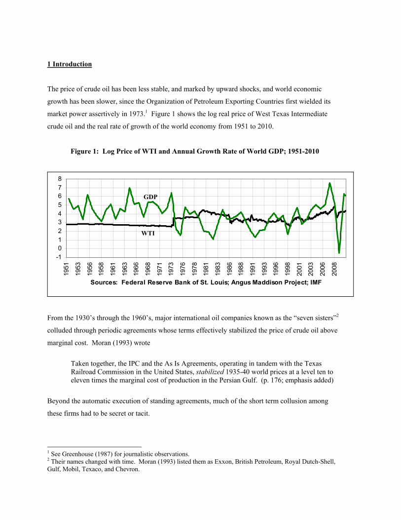
The price of crude oil has been less stable, and marked by upward shocks, and world economic

growth has been slower, since the Organization of Petroleum Exporting Countries first wielded its

market power assertively in 1973.1 Figure 1 shows the log real price of West Texas Intermediate

crude oil and the real rate of growth of the world economy from 1951 to 2010.

Figure 1: Log Price of WTI and Annual Growth Rate of World GDP; 1951-2010

-1012345678

1951

1953

1956

1958

1961

1963

1966

1968

1971

1973

1976

1978

1981

1983

1986

1988

1991

1993

1996

1998

2001

2003

2006

2008

Sources: Federal Reserve Bank of St. Louis; Angus Maddison Project; IMF

From the 1930’s through the 1960’s, major international oil companies known as the “seven sisters”2

colluded through periodic agreements whose terms effectively stabilized the price of crude oil above

marginal cost. Moran (1993) wrote

Taken together, the IPC and the As Is Agreements, operating in tandem with the Texas Railroad Commission in the United States, stabilized 1935-40 world prices at a level ten to eleven times the marginal cost of production in the Persian Gulf. (p. 176; emphasis added)

Beyond the automatic execution of standing agreements, much of the short term collusion among

these firms had to be secret or tacit.

1 See Greenhouse (1987) for journalistic observations. 2 Their names changed with time. Moran (1993) listed them as Exxon, British Petroleum, Royal Dutch-Shell, Gulf, Mobil, Texaco, and Chevron.

GDP

WTI

3

In 1954, sales agreements became the principal focus of the Justice Department's anti-trust case against the oil companies. In 1960, the corporations signed a consent decree promising not to engage in any further explicit market-division practices. (p. 178; emphasis added)

This also stabilized price because the cost of coordinating a change in price secretly or tacitly was

high. The sisters risked uncoordinated changes in price being seen by one another as violations of

contracted, secret, or tacit agreements, rather than as price leadership. OPEC was also founded in

1960. Unlike the sisters, OPEC can meet openly to discuss and agree on changes in price and output.

Individual members can have much more confidence that other members will raise price (cut output)

when they themselves do as part of a price increase that is profitable to the cartel, more confidence

than if the price increase had to be accomplished through secret or tacit cooperation.

...the challenge of maintaining an oligopoly should have been and should continue to be easier for the Organization of Petroleum Exporting Countries (OPEC) than it was for the international oil companies: OPEC can meet and negotiate openly, while the companies had to be furtive and wary of public attack..." (p. 159)

But maintaining an oligopoly and maintaining price are not the same thing. OPEC generally

maintains price above marginal cost in the long run, as the sisters did, but it does not need to accept

an unprofitably stable price in the short run. OPEC can effect changes in price ad hoc.

OPEC has turned its back on, and relinquished access to, the most important mechanisms of restraint the companies managed to impose on themselves. It has systematically unraveled the corporate structure of supra-sovereign limitations, self-denials, and automatic penalties on the members’ own behavior... (p. 161; emphasis added)

Collusion within OPEC in the short run is overt, so it does not have the same stabilizing effect on

price that tacit collusion would. Nor is OPEC constrained by non-OPEC producers from changing

price. OPEC’s unrivaled market power means that it need not hesitate to increase price for fear that

others with market power will quickly raise production and usurp its market share. Non-OPEC

production rises significantly with price in the long run, but is insensitive to price in the short run.

Here, I argue that OPEC as a whole faces a kinked demand curve, because of asymmetric effects of

changes in the price of crude oil on world GDP, not because non-OPEC suppliers have market power.

Increases in the price of crude oil lower world GDP, and, therefore, demand for crude oil, more than

decreases in price raise them. The kink in OPEC’s demand curve implies a vertical discontinuity in

its marginal revenue curve. Within a corresponding range, decreases in production and sales raise

4

price, but reduce revenue by more than they reduce cost, and increases in production and sales lower

price, but raise revenue by less than they raise costs.

Shifts in cost and horizontal shifts in demand cause less instability in price under a kinked demand

curve than under a non-kinked demand curve. With a kinked demand curve, a modest shift in

marginal cost will not change the profit-maximizing quantity of production and sales, or price. A

proportional horizontal shift in demand will also cause no change in price. A parallel horizontal

increase in demand will cause no change or an increase in price, while such a shift always increases

price when there is no kink in demand.3

That said, I still argue that the kink likely has de-stabilizing effects on price that exceed the stabilizing

effects. First, while the kink gives OPEC stronger incentive not to deviate from any

profit-maximizing price/production combination, there is a range of combinations from which OPEC

has such a strong incentive not to deviate, rather than the single such combination that would obtain

without the kink. Thus, modest “cheating” on quotas, disruptions in production, and the like do not

necessarily motivate any stabilizing correction by the cartel. OPEC has been described as “clumsy”.4

The apparent clumsiness may result, in part, from a multiplicity of equilibria in the cartelized market.

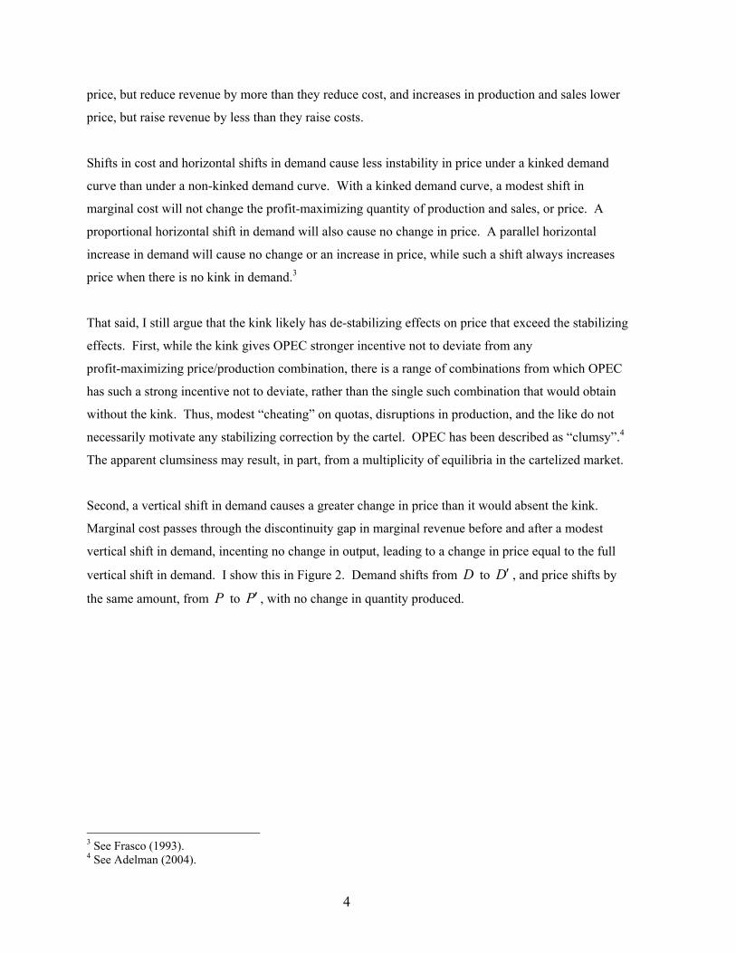
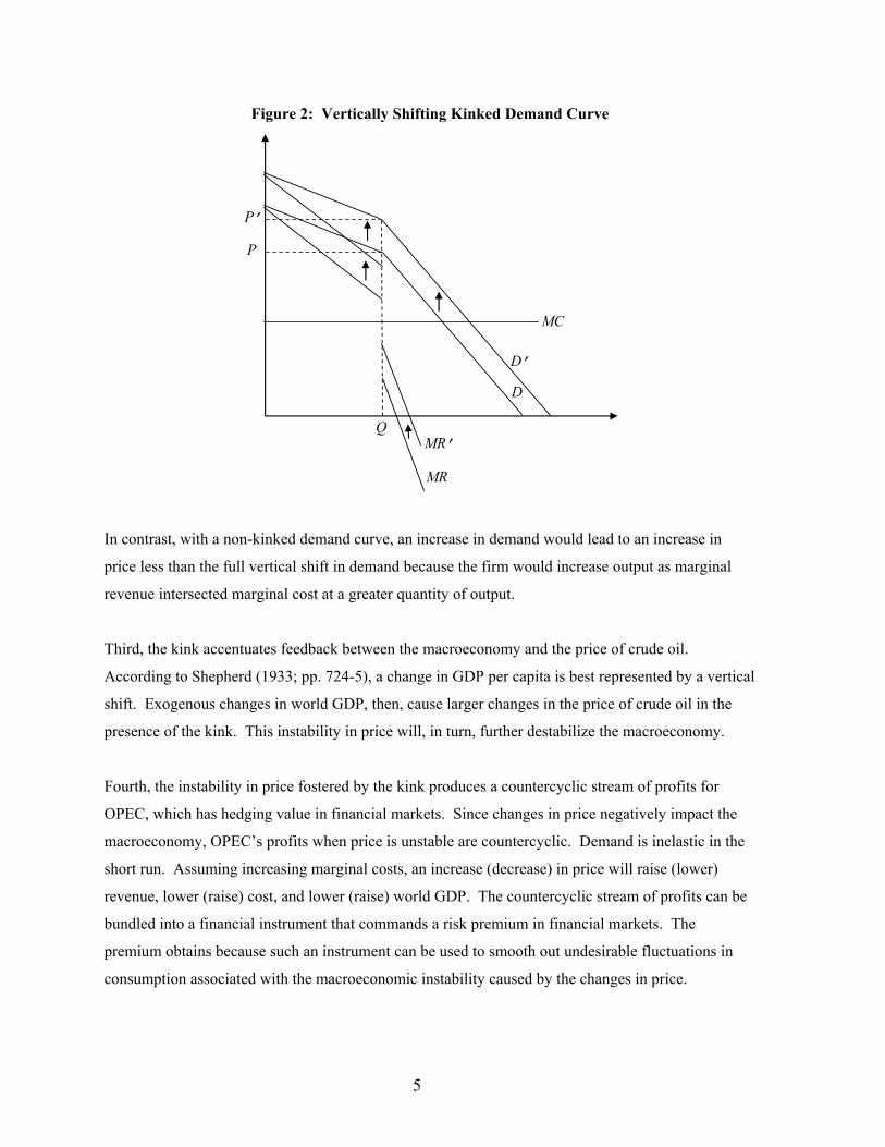
Second, a vertical shift in demand causes a greater change in price than it would absent the kink.

Marginal cost passes through the discontinuity gap in marginal revenue before and after a modest

vertical shift in demand, incenting no change in output, leading to a change in price equal to the full

vertical shift in demand. I show this in Figure 2. Demand shifts from D to D′ , and price shifts by

the same amount, from P to P′ , with no change in quantity produced.

3 See Frasco (1993). 4 See Adelman (2004).

5

Figure 2: Vertically Shifting Kinked Demand Curve

MC

D

P

Q MR’

MR

D’

P’

In contrast, with a non-kinked demand curve, an increase in demand would lead to an increase in

price less than the full vertical shift in demand because the firm would increase output as marginal

revenue intersected marginal cost at a greater quantity of output.

Third, the kink accentuates feedback between the macroeconomy and the price of crude oil.

According to Shepherd (1933; pp. 724-5), a change in GDP per capita is best represented by a vertical

shift. Exogenous changes in world GDP, then, cause larger changes in the price of crude oil in the

presence of the kink. This instability in price will, in turn, further destabilize the macroeconomy.

Fourth, the instability in price fostered by the kink produces a countercyclic stream of profits for

OPEC, which has hedging value in financial markets. Since changes in price negatively impact the

macroeconomy, OPEC’s profits when price is unstable are countercyclic. Demand is inelastic in the

short run. Assuming increasing marginal costs, an increase (decrease) in price will raise (lower)

revenue, lower (raise) cost, and lower (raise) world GDP. The countercyclic stream of profits can be

bundled into a financial instrument that commands a risk premium in financial markets. The

premium obtains because such an instrument can be used to smooth out undesirable fluctuations in

consumption associated with the macroeconomic instability caused by the changes in price.

6

Fifth and finally, though a change in population is better represented by a horizontal shift, if the

macroeconomy is less stable than costs of extracting crude oil and world population, shifts in cost and

demand taken together will cause greater instability in the price of crude oil under a kinked demand

curve than under a non-kinked curve.

OPEC, then, may well find unstable prices more profitable than stable prices.

The Seven Sisters as a whole may also have faced a kinked demand curve, but oil prices were more

stable before 1973 because the Sisters’ collusion had to be tacit, and because of their greater

accountability in general to the government of the United States and other large oil-consuming

nations.

I estimate world demand for crude oil, non-OPEC supply, the effect of crude oil prices on world

GDP, and, therefore, net demand to OPEC. In their survey of literature on energy demand, Atkins

and Jazayeri (2004) discuss three major areas of refinement to the traditional model of demand that

apply to crude oil: asymmetry; regime change; and changing seasonal patterns. Increases in the price

of crude oil affect quantity demanded and GDP differently from decreases. Regarding demand,

according to Atkins and Jazayeri (p. 31), “To say that there is an asymmetry of response appears to be

observationally equivalent to saying that there is some underlying, longer run decrease in demand due

to some kind of energy efficiency of use.” Griffin and Schulman (2005) make a case that a

symmetric specification with a trend toward energy saving technical change is superior. Such a trend

may include deterministic and stochastic elements. Wing (2008; p. 24) states “Of the changes that

occur within industries, disembodied exogenous technical progress is the predominant energy-saving

influence.” I model the direct effects of price on demand as symmetric, and I include both a

deterministic trend and lagged dependent variables in my regression. I allow for asymmetric effects

of crude oil prices on the world economy. In short, I model the market as though all asymmetric

impacts of price on demand result from asymmetric impacts of changes in price on GDP.

Regression analysis of nonstationary time series can produce spurious estimates. Atkins and Jazayeri

argue against the hypothesis of unit roots in oil market data and in favor of multiple structural breaks,

or “regime change”. When modeled as dynamic processes with no changes in intercept or trend,

world GDP and world production, non-OPEC production, and the price of crude oil are nonstationary.

With one major exception, the 1990-91 Gulf War, these apparent nonstationarities are cointegrated by

the estimated coefficients. To the considerable extent that the apparent nonstationarities actually

7

reflect structural breaks, the regressions use most of the information the breaks provide in a way that

leaves stationary residuals and makes economic sense. The exception, as noted, is that I did model

structural breaks in non-OPEC supply around the time of the Gulf War.

Changing seasonal patterns observed in the market for crude oil may be the result of global climate

change. I make no estimate of such a trend, but I purge the data of sample-wide seasonal regularity,

so forecasts based on the estimates do not reflect outdated seasonal patterns in a static sense.

I discuss the data in Section 2. I describe the estimates of world demand for and non-OPEC supply of

crude oil in Section 3, and the effects of crude oil prices on world GDP in Section 4. In Section 5, I

discuss OPEC per se: I calculate net demand to OPEC and present estimated elasticities, marginal

revenue gaps, and ranges of profit-maximizing prices. I conclude in Section 6.

2 Data

Table 1, at end, shows the basic data, various transformations of which I use to make the estimates.

The footnotes to Table 1 explain most of the columns, but Column A is the U.S. refiners’ acquisition

cost of imported crude oil, tabulated and defined by the U.S. Energy Information Administration

(EIA) as the “world price” of crude oil in its analyses and forecasts. I assume that the world market

for crude oil is integrated. According to Adelman (2004; p. 19), “Most oil moves by sea, and ships

can be diverted from one destination to another relatively easily. Moreover, much additional oil can

be diverted from land shipment to sea. Hence, it is fairly easy to reroute shipments of oil from

nations that have a sufficient supply to nations that are experiencing a shortage. It is only a minor

exaggeration to say that every barrel in the world competes with every other.”

8

Between early 2011 and mid-2013, oil prices in the North American interior, as measured by the

West Texas Intermediate (WTI) New York Mercantile Exchange (NYMEX) benchmark, fell relative

to their historic relationship with oil prices elsewhere. Historically high world prices made large

quantities of unconventional crude oil economically recoverable. The additional production

congested pipelines between Cushing, OK, where the benchmark is priced, and the U.S. Gulf Coast,

separating WTI from the world market. The Brent-WTI split stood at $6.31/bl as of March 6, 2014,

much narrower than its $27.31/bl average in September, 2011, but still higher than its, slightly

negative, historical norm.5

The separation in markets extended to that for retail products. Figure 3 shows the Brent – WTI split

(in $/bl) along with the difference between the simple average of retail gasoline prices (in ¢/gallon)

across PADDs 1, 3, and 5 (U.S. coastal areas) and that across PADDs 2 and 4 (U.S. interior).6 As the

Brent – WTI split became large, so did the difference in gasoline prices. A regression of the

difference in gasoline prices on the split, monthly dummies, and twelve lags of the dependent variable

gives a coefficient on the split with a t-statistic of 2.14; there is no autocorrelation in the residuals.

When the split is small, so is its effect on gasoline prices, but in September 2011, this coefficient

implies an elasticity of the difference in gasoline prices with respect to the Brent – WTI split of 0.45,

which is significant. I conclude that the North American interior has been a distinct and separate

market for crude oil and products since early 2011, and I do not use data from after 2010 in my

analysis. Apart from its simplicity, this way of dealing with the fragmentation of the market in recent

years means that when I later apply the estimates in a more current (2014) context, I am doing so well

out of sample, a good test of the accuracy of a model.

5 More information is available at http://www.eia.gov/todayinenergy/detail.cfm?id=11891, accessed July 15, 2013. 6 “PADD” stands for “Petroleum Administration Defense District”. See http://www.eia.gov/todayinenergy/detail.cfm?id=4890, accessed March 6, 2014, for a map.

9

Figure 3: Brent - WTI Split and U.S. Regional Gasoline Prices

-20

-10

0

10

20

30

40

5019

93

1994

1995

1995

1996

1997

1998

1999

2000

2000

2001

2002

2003

2004

2005

2005

2006

2007

2008

2009

2010

2010

2011

2012

2013

PADDs 1, 3, & 5 less PADDS 2 & 4 Brent less WTI

Source: U.S. Energy Information Administration, http://tonto.eia.gov/dnav/pet/hist/LeafHandler.ashx?n=PET&s=EMM_EPM0_PTE_R10_DPG&f=M, accessed March 6, 2014. I estimate the price of crude oil for October-December of 1973 based on monthly data on the rest of

this series and free-on-board and landed costs of crude oil imported to the U.S. from January 1974 to

April 2009. The prices of crude oil for October-December 1973 used to calculate the quarterly

average, highlighted in yellow in Table 1, are predicted values based on the following regression:

0.0276 0.0828 0.08560.0083 0.5037 0.5435world fob landed

t t tP P P∆ = − + ∆ + ∆ (1)

where t is in months, worldtP∆ is the month-to-month change in the world price, fob

tP∆ the change in

the free-on-board price, and landedtP∆ the change in the landed price. The 2 0.9640R = . A dynamic

process can be described as ( )I d , where 1d = corresponds to a unit root and 0d = to perfect

covariance level stationarity. A generalization of this distinction is to allow d to assume non-integer

values. Robinson tests7 estimate the degree of fractional differencing, d, needed to render an I(d)

series I(0) using a log-periodogram regression. According to Baillie (1996; p. 21), “For

0.5 0.5d− < < , the process is covariance stationary, while 1d < implies mean reversion.” A

7 See Robinson (1995).

10

Robinson test of the residuals in (1) estimates them to be ( )0.04350.2173I − , where the number below is

the standard error of the estimate.

Column H is the percent drop in world output of crude oil caused by war or civil conflict. The

episodes of war and civil conflict include the November 1973 Yom Kippur war, the November 1978

onset of the Iranian Revolution, the October 1980 onset of the Iran-Iraq war, the August 1990 Iraqi

invasion of Kuwait, civil unrest in Venezuela beginning in December 2002, and the U.S. invasion of

Iraq in March of 2003.

I derived real crude oil prices using Columns A and B.

I derived quarterly world GDP by applying quarterly variation in U.S. GDP, Column F, to annual

world GDP, Column E. Both U.S. GDP and U.S. consumption of crude oil declined from a fourth to

a fifth of the worldwide totals, and the oil intensity of the U.S. economy was about the same as that of

the world economy, throughout the sample. I used world GDP rather than OECD GDP as a measure

of income. The non-OECD share of world consumption of crude oil has increased from 25% to 50%

since 1970.8 Rapid economic growth has caused demand for oil to grow especially fast in some

non-OECD countries such as China and India. I used purchasing power parity (PPP) because market

exchange rates are subject to political and speculative influences that do not reflect the real incomes

of consumers of crude oil and those affected by the market for it. National GDPs calculated using

market exchange rates can deviate from purchasing power parity for extended periods.9

For each series in Table 1, I either used seasonally adjusted data, made adjustments for seasonality, or

found no seasonal variation when regressing them on seasonal dummy variables, so I made no

seasonal adjustments. I made no adjustments to my methods of estimation to account for the extent to

which the data used were estimated or constructed.

8 Source: U.S. Energy Information Administration, http://www.eia.gov/finance/markets/demand-oecd.cfm, accessed March 7, 2014. 9 See Cashin and McDermott (2001).

11

2.1 Seasonal Adjustment

I removed seasonal variation in world production, non-OPEC production, and price in the following

manner: I regressed each series and its first differences on seasonal dummy variables; I added the

residuals from each regression to the mean of the dependent variable to get preliminary seasonally

adjusted levels and first differences, respectively; I added the cumulative sum of the preliminarily

seasonally adjusted first differences to the initial value of the preliminarily seasonally adjusted levels

to get secondarily seasonally adjusted levels; I added a constant to the secondarily seasonally adjusted

levels so that the mean of the resulting series was the same as that of the original series; this gave me

a final seasonally adjusted series. I found that this extensive process was necessary to purge both the

series and their first differences of regular seasonal variation, as measured by the (in)significance of

the coefficients when the final series and their first differences were regressed on seasonal dummy

variables.

3 World Demand for and Non-OPEC Supply of Crude Oil

I assume that the quantity of crude oil demanded equals the quantity supplied, as measured by world

production of crude oil. The quantity demanded, then, includes that amount added to inventory.

3.1 Specification of World Demand

I estimate quarterly world demand for crude oil as a linear function of a constant, price, world GDP, a

linear time trend, one lag of quarterly quantity demanded, and annual quantity demanded lagged one

quarter:

0 1 1D

t P t G t D t Dave t tD P G t D Daveδ δ δ δ δ δ ε− −= + + + + + + (2)

tD is quarterly quantity of crude oil demanded worldwide in billion barrels per year, tP is the real

price of crude oil in 2005$/bl, tG is world gross domestic product (purchasing power parity;

normalized to average 1 in 2005), t is time in quarters (t = 0 in 2011:II), 1tDave − is annual demand

12

for crude oil for the four quarters ending with quarter 1t − , and Dtε is potentially heteroskedastic,

autocorrelated, and correlated with Stε from (3), below.

The price term Pδ captures the effect of contemporaneous price on the quantity of crude oil

demanded worldwide. I treated quantity demanded as a linear function of price so that the price

elasticity of demand would increase with price. Numerous substitutes for crude oil, including

potential conservation measures, exist, but they have only become competitive as oil prices have

reached new highs. These may include ethanol from cellulose as well as corn, biodiesel, coal to

liquids, natural gas to liquids, potentially huge reserves of natural gas hydrates below the ocean floor,

nuclear power, wind power, photovoltaic solar power, electric cars, and denser urban design. The

choice of price rather than log price as a regressor, then, is motivated by the assumption that greater

competitiveness of alternatives to crude oil increases the price elasticity of demand for crude oil as

the price reaches new highs. If price trends up faster than demand, the associated percentage drop in

quantity demanded increases as the price increases. Adelman (1990; p. 11) wrote “…the higher the

price, the greater the incentive to consumers to substitute other comparable goods; and to producers,

to substitute labor and capital or other inputs. In addition, for both consumers and firms, there is an

income effect pushing the same way: the greater the importance of the product in the total budget, the

more important the impact of a further increase. Hence the higher the price, the greater the response

to a given price change.” Statistically, price performed better than log price in specification tests.

I include a time trend to account for increasing efficiency in the use of crude oil. From Table 1, the

ratio of world crude oil consumption to GDP in 2009 was a fifth of what it was in 1974. While some

of this resulted from substitution of other fuels for oil, most did not. In 2010, worldwide consumption

of primary energy of all kinds per unit of GDP was a fourth of what it was in 1980.10 According to

Atkins and Jazayeri, inclusion of the time trend obviates the need to model the direct effects of price

on demand as asymmetric, since the two are observationally equivalent. According to Griffin and

Schulman, the trend is superior. According to Wing, the deterministic trend is important, at least in

the U.S.

I model persistence in demand for crude oil using both quarterly and annual quantity demanded of

crude oil lagged one quarter; 1tD − and 1tDave − . Rather than using a series of quarterly lags, I use an

10 Source: U.S. Energy Information Administration; http://www.eia.gov/cfapps/ipdbproject/IEDIndex3.cfm?tid=44&pid=44&aid=2, accessed July 15, 2013.

13

annual average to emphasize long term persistence.11 Short term persistence results from rigidity in

planning for the use of oil-specific capital and durables, such as travel planning. Long term

persistence results from the sunk costs of large amounts of substantially oil-specific physical and

human capital and durables, beginning at the refinery and continuing downstream to such things as

gasoline-powered vehicles and auto-oriented urban design. The sunk costs make maintenance of

existing capital cheaper than replacement with new capital better optimized to a current price of crude

oil. Both “short term” and “long term” persistence are short run phenomena, in that there are no sunk

costs of oil-specific capital and durables, and, therefore, no persistence, in the long run. Although its

coefficient is only statistically significant at the “85% level” in the regression below, including

1tDave − improves the model’s performance in specification tests.

3.2 Specification of Non-OPEC Supply

I modeled non-OPEC supply as a linear function of a constant, a dummy variable for the quarters

surrounding the Gulf War, log price, cumulative non-OPEC supply lagged one quarter, a one quarter

lag in interest on three-month U.S. treasury bills, a one quarter lag in the trade-weighted exchange

value of the U.S. dollar, a linear time trend, and quarterly non-OPEC production lagged one quarter.

90 92

0 1 1 1 1III IV S

t GW t p t CS t i t X t S t tS M p C i X t Sη η η η η η η η ε− − − −= + + + + + + + + (3)

where tS is quarterly non-OPEC quantity supplied, 90 92III IVtM is a dummy variable equaling 1 from

1990:III through 1992:IV, lnt tp P≡ is log price, 1tC − is cumulative non-OPEC production lagged

one quarter, 1ti − is interest on three-month U.S. treasury bills lagged one quarter, 1tX − is the

trade-weighted exchange value of the U.S. dollar lagged one quarter, t is a linear trend measured in

quarters and equaling zero in 2011:II, and Stε is potentially heteroskedastic, autocorrelated, and

correlated with Dtε from (2).

Iraqi and Kuwaiti production fell during and after the Gulf War, the International Energy Agency

tapped strategic stocks, expectations changed significantly and frequently, and short term volatility in

price increased at the time of and following Iraq’s August 1990 invasion of Kuwait. Allowing a

11 This also keeps down the number of regressors and, therefore, the variances of the estimates.

14

temporary shift in intercept during this time improved the results of tests of specification and

stationarity.

I use log price so that the price elasticity of non-OPEC supply decreases in quantity supplied. While

many sources of crude oil may be available, there is substantial variability in the cost of extracting

and finding them. The decreasing short run elasticity reflects the effect of increasing costs of

extraction as existing sources are used more intensively. Decreasing long run elasticity and lagged

cumulative supply reflect increasingly costly sources being exploited.

The U.S. interest and exchange rates reflect the importance of the U.S. dollar to commodity markets

in general and that for crude oil in particular. Both organized exchanges and contracts for crude oil

typically quote prices in dollars. The dollar was the world’s “petro-currency” throughout the sample

period and remains so today. The nominal rate of interest on dollar-denominated securities

essentially measures the degree of inflationary expectation for the U.S. economy: The “real interest

rate” component measures the extent to which the Federal Reserve tightens credit to prevent inflation,

and the remaining component represents the extent to which it accommodates inflation. A change in

the exchange value of the dollar can affect the incentive to produce under non-indexed lease

agreements and forward contracts, but it will only shift demand for crude oil between the U.S. and

other countries, without having much affect on world demand, since the U.S. economy is about as

oil-intensive as the world economy as a whole. Empirically, if I include 1ti − and 1tX − in the demand

equation, both when retaining them in and when removing them from the supply equation, they are

not at all statistically significant in the demand equation.

The time trend captures the effect of advancing technology of exploration, development, and

extraction. Lagged quantity supplied reflects persistence in supply resulting from the presence of

physical and human capital specific to exploration and extraction of crude oil.

I tried including an annual moving average term lagged one quarter, 1tSave − , like 1tDave − in (2), in

(3). While including 1tDave − in (2) improved the results of specification tests, excluding 1tSave −

improved the results of specification tests. The re-optimization of investment in exploration and

extraction in response to changes in the price of crude oil is less complicated than that of the capital,

durables, and other factors used in combination with crude oil, so long term persistence does not

warrant emphasis in a separate variable in the case of non-OPEC supply, as it does in demand.

15

3.3 Identification and Estimation of World Demand and Non-OPEC Supply

Identification of world demand and non-OPEC supply is the most challenging aspect of making these

estimates. I treat the price term in (2) as an endogenous regressor because innovations in demand can

cause contemporaneous changes in price. I treat log price in (3) as endogenous because it depends on

shifts in supply. I also treat GDP, in (2), as endogenous because, for example, a war could affect both

demand for crude oil and GDP. Price and log price are codetermined, so there are, effectively, two

endogenous regressors in the system.

Finding excluded instruments that are both strong and exogenous to a global market with

macroeconomic externalities is difficult to do perfectly. I use one- and two-year (i.e. four and eight

quarter) lags of disruptions in world supplies of crude oil resulting from war or civil conflict, 4tQ −

and 8tQ − , and one- and two-year lags of world GDP, 4tG − and 8tG − . All of the excluded

instruments are lagged and, therefore, not causally impacted by innovations in demand for or supply

of crude oil. Hamilton (2003) uses disruptions to crude oil supplies to extract variation in price that

was exogenous to U.S. GDP. The variable tQ is the percent drop in world supply of crude oil during

Quarter t associated with the episodes listed in the description above of Table 1, all of which occurred

in OPEC countries. It is an extension of Hamilton’s instrument. tQ represents changes in OPEC

production associated with conflict.

Lagged GDP is a strong instrument for current GDP, and it is unlikely that the four- and eight-quarter

lags would correlate with current demand without also correlating with lagged demand, which is well

controlled for in (2). More generally, because current and lagged market quantities, prices, incomes,

and technological change are controlled for as well, the excluded instruments correlate with these

and, therefore, need not correlate with the current error term. In a recursive dynamic process such as

that followed by demand in (2), lagged values of the regressors affect the dependent variable through

its lags in a way that declines geometrically with the length of the lag. When lagged GDP affects

lagged price, it will also, in turn, affect current demand through lagged demand. GDP can be

modeled as having its own recursive process, but its dynamics are modeled in a manner in the

recursive process describing demand, as well. Finally, inasmuch as, beyond these effects, lagged

GDP still affects the error term, it will likely have a greater effect on lagged errors than current ones,

16

and these effects will also be captured in the dynamic process followed by demand. The current error

term, Dtε , may be unaffected if it is not correlated with lagged errors; Figure 4, below, shows no 95%

statistically significant autocorrelation in the residuals from estimation of (2), and the p-value in a

Portmanteau’s Q test of the null hypothesis that the residuals associated with (2) are white noise is

0.9985. In sum, Equation (2) substantially provides ways for 4tG − and 8tG − to affect tD through

8...1Dtε − , 7...0tG − , 8...0tP− , 8...1tD − , and 8...1tDave − , rather than through D

tε , and there is no evidence of

correlation between 8...1Dtε − and D

tε . Furthermore, the p-value in a Sargan test of the joint null

hypothesis that 4tG − , 8tG − , 4tQ − , and 8tQ − are uncorrelated with Dtε and S

tε and correctly excluded

from (2) and (3) is 0.69. Perhaps most tellingly, in a first stage regression of tD on all exogenous

variables, neither 4tG − nor 8tG − is statistically significant ( 0.04 and 0.77t = − , respectively), while

1tD − is highly significant ( 6.92t = ).

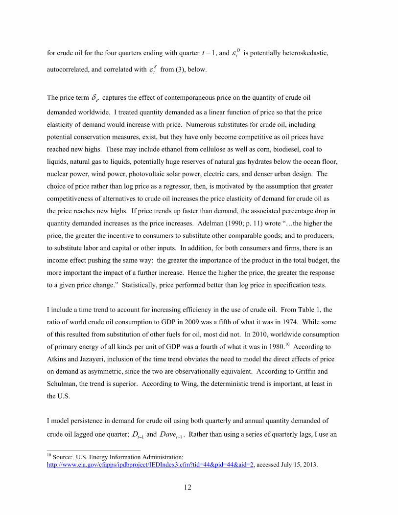
3.4 Results and Testing of Estimated World Demand and Non-OPEC Supply

Three stage least squares accounts for correlations in errors across equations. I used ®Stata’s reg3

command to estimate Equations (2) and (3) simultaneously using iterated generalized least squares. 12

The estimates, shown in Equations (4) and (5), converged in five iterations.

1 11.6155 0.0044 0.0184 0.0362 0.0956 0.1010-1.7283 0.0125 0.0441 0.0715 0.7655 0.1526 D

t t t t t tD P G t D Dave e− −= − + − + + + (4)

90 92

13.2638 0.0385 0.0764 0.0086

1 1 10.1479 0.0162 0.0892 0.0192

8.1301 0.0750 0.2376 0.0227

0.3520 0.0416 0.2211 0.9416

III IVt t t t

St t t t

S M p i

X C t S e

−

− − −

= − + −

+ − + + + (5)

The 2 0.99R = for demand and 0.98 for non-OPEC supply. All of the coefficients are significantly

different from zero at the 99% level except: the Gulf War dummy variable, which is significant at the

90% level; the demand constant, which is not significant; the deterministic trend in demand, which is

significant at the 95% level; and 1tDave − , which is “significant at the 85% level”. Portmanteau’s Q

12 I performed my calculations using Stata/SE Version 10.1 for Windows.

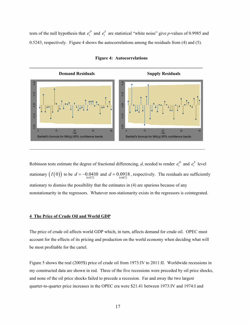
17

tests of the null hypothesis that Dte and S

te are statistical “white noise” give p-values of 0.9985 and

0.5243, respectively. Figure 4 shows the autocorrelations among the residuals from (4) and (5).

Figure 4: Autocorrelations

_____________________________________________________________________________

Demand Residuals Supply Residuals

-0.2

0-0

.10

0.00

0.10

0.20

0 10 20 30 40Lag

Bartlett's formula for MA(q) 95% confidence bands

-0.2

0-0

.10

0.00

0.10

0.20

0 10 20 30 40Lag

Bartlett's formula for MA(q) 95% confidence bands

______________________________________________________________________________

Robinson tests estimate the degree of fractional differencing, d, needed to render Dte and S

te level

stationary ( )( )0I to be 0.0572

0.0410d = − and 0.0872

0.0918d = , respectively. The residuals are sufficiently

stationary to dismiss the possibility that the estimates in (4) are spurious because of any

nonstationarity in the regressors. Whatever non-stationarity exists in the regressors is cointegrated.

4 The Price of Crude Oil and World GDP

The price of crude oil affects world GDP which, in turn, affects demand for crude oil. OPEC must

account for the effects of its pricing and production on the world economy when deciding what will

be most profitable for the cartel.

Figure 5 shows the real (2005$) price of crude oil from 1973:IV to 2011:II. Worldwide recessions in

my constructed data are shown in red. Three of the five recessions were preceded by oil price shocks,

and none of the oil price shocks failed to precede a recession. Far and away the two largest

quarter-to-quarter price increases in the OPEC era were $21.41 between 1973:IV and 1974:I and

18

$22.04 between 2008:I and 2008:II. There was a slowdown in the world economy in 1974:II, a

recession beginning in 1974:III, and a recession beginning in 2008:III. The third largest increase in

price during the OPEC era of $12.63 occurred between 2007:III and 2007:IV. The large shock in

1973 preceded a long term slowdown in world economic growth, and the 2008 recession has been

termed “Great”. Over two quarters, from 1978:III to 1980:I, price increased $39.51. GDP declined at

an annual rate of more than 8% from 1980:I to 1980:II and 0.7% the following quarter.

Figure 5: Real (2005$) Price of Crude Oil from 1973:IV to 2011:II

020

4060

8010

0

1972 1977 1982 1987 1992 1997 2002 2007 2012

4.1 Specification of World GDP

A good deal has been written about asymmetry in the response of the macroeconomy to changes in

the price of crude oil.13 Increases in price damage the economy more than decreases help. To

illustrate one reason why, suppose wages are sticky in the downward direction. Figure 6 describes

the market for labor when the price of crude oil fluctuates.

19

Figure 6: Labor Market with Downwardly Sticky Wages and Fluctuating Price of Crude Oil

The price of crude oil changes from 0P to 1P (not shown), raising the cost of fuel used to travel to

work and back, shifting the competitive supply of labor from 0LS to 1

LS . The equilibrium wage

increases from 0W to 1W , and the quantity of labor demanded decreases from 0L to 1L . Next, the

price of crude oil returns to 0P , but workers continue to require wage 1W , so the supply curve

changes to SLS , the quantity of labor supplied remains at 1L , and less output is produced than before

the price of crude oil increased and subsequently decreased to its original level.

To capture the asymmetric effects econometrically, I specify increases and decreases in the price of

crude oil separately, using first differences in log price to explain first differences in log GDP. With

this functional form, regression coefficients represent the, constant, elasticities of GDP with respect to

the price and lagged prices of crude oil. I allow for response in the first difference in the log of GDP

to zero through five quarter lags in increases and decreases in the log price of crude oil. I also include

five lagged dependent variables, first differences in log GDP, in the regression.

( ) ( ) ( )1 1

1 0 1 1 15 5 5

max ,0 min ,0t t t

g gt t s s s s s s s s s t

s t s t s tg g p p p p g gγ γ γ γ ε

− −+ −

− − − −= − = − = −

− = + − + − + − +∑ ∑ ∑ (6)

13 See, for example, Hamilton (2003), Greene and Ahmad (2005), or Gately and Huntington (2002).

1W

1L

SLS

LD

L

1LS

0L

W

0W

0LS

20

where tg is the natural logarithm of world GDP in quarter t, ( tG , (normalized to 100 in 2005),

lnt tg G≡ ), and gtε is a potentially heteroskedastic and autocorrelated error. With the lagged

dependent variables, changes in price beyond the fifth lag may impact current GDP. The lag structure

is just long enough to include the lag with the largest impact. Impacts through the lagged dependent

variables decline with their distance in time from t .

4.2 Identification of World GDP

I treat contemporaneous changes in log price, ( )1max ,0t tp p −− and ( )1min ,0t tp p −− as

endogenous because GDP can affect current price. The excluded instruments include lags of

positive and negative differences between the residuals from the demand and non-OPEC supply

equations (unexplained changes in OPEC production), specified separately, ( )1 1max ,0D St te e− −− and

( )1...3 1...3min ,0D Ss t s te e= − = −− . In first-stage regressions, only the first lag of the positive changes in

unexplained OPEC production was significant, while the first three lags of negative changes were, so

I did not use the longer lags of the positive changes. One interpretation is that the cooperative game

among OPEC members in which prices are raised through cuts in production must be repeated to

succeed; cooperation is easier to establish in repeated than in one-shot cooperative games. On the

other hand, when OPEC wants prices to fall, it may simply allow cooperation to break down, and this

can be done quickly and easily.

Estimates of coefficients are consistent in OLS regressions with “generated regressors”. In 2SLS, the

transformations of D St s t se e− −− are “generated instruments”. According to Wooldridge (2002; p. 117),

“…there are practical reasons for using 2SLS with generated instruments rather than OLS with

generated regressors.” Whether the generated instruments are included or excluded, inference using

heteroskedasticity- and autocorrelation-robust standard errors in a GMM context, a generalization of

both OLS and 2SLS done here, is consistent and asymptotically efficient.

I assume that OPEC producers are the only strategic decision-makers impacting the price of crude oil,

and the price of crude oil impacts world GDP. Thus, OPEC production is a driver of both the price of

crude oil and world GDP, through price. This does not mean that OPEC producers do not also

21

respond to GDP, but lagged OPEC production would only depend on current innovations in GDP

through accurate expectations of those innovations. The innovations in (6) are independent of lagged

changes in price and GDP. I assume that OPEC producers are not able to anticipate these

innovations.

The excluded instruments for contemporaneous changes in log price also include a dummy variable

equaling 1 from the beginning of the dataset through 1985:I, 1985ItM . The assumed shift in volatility

of price in 1985:II coincides with the maturation of crude oil as an actively traded commodity. The

coefficient of determination (standard deviation over mean) of price equals 0.30 through 1985:I and

0.57 thereafter. Verleger (2005; p. 5) explains that as prices dropped in the early 1980’s, the world

crude oil market was in transition from a vertically integrated one to one characterized by active

commodity markets. In particular, “...the development of North Sea production introduced classic

commodity market institutions into the global oil market. A true spot market was created.” The

development of the commodity market preceded, and facilitated, the “price collapse of 1986”, which

likely resulted from OPEC’s increasing excess capacity associated with falling short term demand.

Examples of dummy variables as excluded instruments can be found in Evans and Schwab (1995) and

Djankov and Reynal-Querol (2007).

22

4.3 Results and Testing of Estimated World GDP

Continuously updated GMM estimates of (6), shown in Table 2, converged after 153 iterations.

Table 2: Estimated Effects of Changes in Crude Oil Prices on the First Difference in

World GDP, 1t t tg g g −∆ ≡ −

__________________________________________________________________________________________

Coefficient Standard. Error Coefficient Standard. Error

tp+∆ -0.086 0.020 1tg −∆ 0.181 0.116

tp−∆ -0.039 0.016 2tg −∆ -0.053 0.042

1tp+−∆ 0.012 0.006 3tg −∆ -0.293 0.063

1tp−−∆ 0.016 0.008 4tg −∆ 0.463 0.121

2tp+−∆ -0.009 0.008 5tg −∆ 0.001 0.077

2tp−−∆ -0.011 0.007 Constant 0.009 0.002

3tp+−∆ -0.006 0.005

3tp−−∆ -0.003 0.005

4tp+−∆ 0.005 0.004

4tp−−∆ -0.015 0.010

5tp+−∆ -0.021 0.005

5tp−−∆ -0.014 0.004

__________________________________________________________________________________________

1s s sg g g −∆ = − is the quarterly first difference in the natural logarithm of world GDP.

( )1max ,0s s sp p p+−∆ ≡ − is the positive change in the natural log price of crude oil between

Quarter 1s − and Quarter s , and ( )1min ,0s s sp p p−−∆ ≡ − the negative change.

Of the 18 regressors, including the constant, six have coefficients that are significantly different from

zero at the 99% level, two others at the 95% level, and one more at the 90% level. I retained the

remaining nine so as to maintain the contiguity and consistency of the lag structure. The test statistics

are robust to heteroskedasticity and autocorrelation of any form. However, A Pagan-Hall test using

23

the predicted values, ˆ tg , associated with Table 2 as an indicator variable fails to reject

homoskedasticity in the errors ( )0.970p = . There is no statistically significant autocorrelation in

the residuals at any specific lag, as shown in Figure 7, and a Cumby-Huizinga test fail to reject a null

hypothesis that there is no autocorrelation at any lag up to 25 ( )0.985p = .

Figure 7: Autocorrelations Among GDP Residuals

-0.2

0-0

.10

0.00

0.10

0.20

0 10 20 30 40Lag

Bartlett's formula for MA(q) 95% confidence bands

A Bartlett cumulative periodogram test puts a p-value of 0.857 on a null hypothesis that the residuals

were generated by a white noise process. They are stationary; 0.075

-0.009Estimated d = in a Robinson

test.

There are five excluded instruments and two endogenous regressors in a dataset of 158 observations,

used to perform a regression with five lags in the regressors. The p-value in a Hansen test of a null

hypothesis that the excluded instruments are independent of the error term is 0.882. When I omit

( )1 1max ,0D St te e− −− and ( )1 1min ,0D S

t te e− −− from the set of instruments, the p-value is 0.515, and

when I test a null that ( )1 1max ,0D St te e− −− and ( )1 1min ,0D S

t te e− −− are independent of the error term,

assuming the other excluded instruments are also, the p-value is 0.888. The value of a

24

Kleibergen-Paap Wald rk F-statistic is 23.80, which exceeds the highest, 90%, critical value reported

by Stata of 4.32, leading to a rejection of a null hypothesis that the excluded instruments are weak.

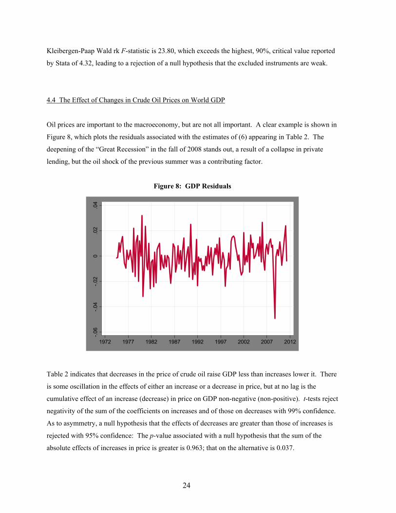
4.4 The Effect of Changes in Crude Oil Prices on World GDP

Oil prices are important to the macroeconomy, but are not all important. A clear example is shown in

Figure 8, which plots the residuals associated with the estimates of (6) appearing in Table 2. The

deepening of the “Great Recession” in the fall of 2008 stands out, a result of a collapse in private

lending, but the oil shock of the previous summer was a contributing factor.

Figure 8: GDP Residuals

-.06

-.04

-.02

0.0

2.0

4

1972 1977 1982 1987 1992 1997 2002 2007 2012

Table 2 indicates that decreases in the price of crude oil raise GDP less than increases lower it. There

is some oscillation in the effects of either an increase or a decrease in price, but at no lag is the

cumulative effect of an increase (decrease) in price on GDP non-negative (non-positive). t-tests reject

negativity of the sum of the coefficients on increases and of those on decreases with 99% confidence.

As to asymmetry, a null hypothesis that the effects of decreases are greater than those of increases is

rejected with 95% confidence: The p-value associated with a null hypothesis that the sum of the

absolute effects of increases in price is greater is 0.963; that on the alternative is 0.037.

25

The asymmetry in Table 2 echoes that in a number of estimates. Hamilton (2003) explains the

asymmetry in the relationship as the result of allocative disturbances and uncertainty. An unexpected

change in oil prices in either direction changes the optimal mix of industrial equipment and consumer

durables that firms and consumers, respectively, desire. If the change makes them uncertain about the

future direction of prices, then they are likely to postpone major purchases until the uncertainty is

resolved. This would also apply to governments, in particular with regard to transportation

infrastructure and urban planning. (Hamilton (2009; pp. 39-40) notes “…house prices in 2007 were

likely to rise slightly in the zip codes closest to the central urban areas but fall significantly in zip

codes with longer average commuting distances.”) Thus, there is a contractionary element in the

effects of either increases or decreases in the price of crude oil, but no corresponding expansionary

element in the effects of increases.

Another reason for the strong asymmetry is downward stickiness of wages in the short run, as shown

in Figure 6, which illustrates effects through the supply of labor. Demand for labor may also shift.

When the price of oil rises, to the extent that labor and oil are complements, demand for labor falls,

causing only unemployment. To the extent that labor and oil are substitutes, demand for labor rises,

raising wages and employment. When the price of oil falls, to the extent that labor and oil are

complements, demand for labor rises, raising wages and employment. To the extent that labor and oil

are substitutes, demand for labor falls, causing only unemployment. There is no reason before the

fact to suppose that the sum of these effects is zero. Most workers in countries that are not poor use

oil products or close substitutes, such as natural gas, to travel to and from work, so oil is related to

labor in the production of a large majority of goods. Other inputs related to oil in production of goods

may also have downwardly sticky prices, and this may contribute to the asymmetry.

A third reason for the asymmetry is income and liquidity effects. Since oil products and their

substitutes take a large share of many budgets, increases from a given price level reduce spending

more than decreases from that level increase spending. These effects can be especially strong in poor

countries. Teitenberg (2007; p. 202) writes “The lack of foreign exchange has been exacerbated

during periods of high oil prices. Many developing nations must spend large portions of export

earnings merely to import energy.

Fourth, investors whose wealth and income are sensitive to the price of oil will hold increases therein

in liquid form for a time before committing to a less liquid investment. A large change in price in

26

either direction will redistribute wealth and income and, as a result, tend to slow down real

investment.

Consider the response in GDP in Quarter t to a change in price s quarters earlier. From (6), the

short run elasticity of world GDP s quarters hence with respect to a change in price lasting one

quarter is

/

2

t tgt

i jj t s ii t st s

gp

γ γ+ −

= − −= −−

∆= ∆ ∑ Π

where 1gtγ ≡ and /

iγ+ − is the coefficient on an increase/decrease in log price in Quarter i and g

jγ

the coefficient on the change in log GDP in Quarter j.

Evaluating this at 5s = in 2009:III gives an estimate of the impact of the large increase going into

summer 2008. Price (2005$) in 2008:II was 5 $106.31tP− = , and in 2008:I was 5 1 $84.05tP− − = .

The estimated elasticity is -0.0203, and the price change was 23.5%, so the estimated effect is that

world GDP was 0.48% lower in 2009:III due to that largest ever quarter-to-quarter increase in the real

price of crude oil. In my constructed data, world GDP was 2.14% lower in 2009:III than in 2008:II,

so Table 2 implies that a fifth of the decrease was caused by the upward shock in 2008:II. The oil

shock contributed significantly to the Great Recession, but was not its primary cause.

These negative short run effects reduce GDP in the long run because lower current GDP means lower

current investment, which is the only way to provide now for future GDP. Short run dips in GDP

lower future GDP because investment varies directly and elastically with GDP. Hysteresis also sets

in among unemployed workers, lowering their future productive capability; a recession in

employment implies less current investment in human capital through accumulation of work

experience. The long run elasticity of world GDP with respect to a temporary, one quarter, change in

the price of crude oil is

5 51

5

0.056 using Table 2.1

t ti ii t i t

t gii t

γ γ

γ

+ −= − = −

−

= −

−≈ −

−∑ ∑

∑

27

A 1% increase in the price of crude oil lasting exactly one quarter lowers world GDP in the long run

by 0.056% . Thus, if it had been exactly reversed in 2008:III, the largest-ever, $22.27/bl in 2005$,

increase the previous quarter would have caused world GDP to be 1.32% lower in each quarter over

the long run. In my constructed data, world GDP grew about 1.96% quarterly. The shock of 2008,

then, set the world economy back about two months.

5 OPEC

The supply curve of a monopolist does not exist. OPEC is not a monopolist in the literal sense, but its

market power in the world market for crude oil is unrivaled, so, as a whole, its profit-maximization

problem is like that of a monopolist. OPEC does not interact strategically with non-OPEC suppliers,

with the possible exceptions, ignored here for simplicity, of the governments of Mexico, Norway, and

Russia; OPEC takes account of its influence on non-OPEC production when deciding its own

production, but non-OPEC producers do not take account of their influence on OPEC in deciding

their production14. Since OPEC’s market power is substantial and unrivaled, it decides the world

price of crude oil as it decides its own production.

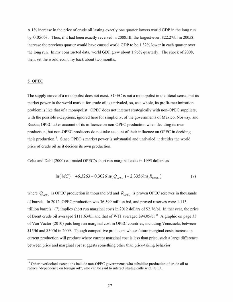
Celta and Dahl (2000) estimated OPEC’s short run marginal costs in 1995 dollars as

( ) ( ) ( )ln 46.3263 0.3026ln 2.3356lnOPEC OPECMC Q R= + − (7)

where OPECQ is OPEC production in thousand b/d and OPECR is proven OPEC reserves in thousands

of barrels. In 2012, OPEC production was 36.599 million b/d, and proved reserves were 1.113

trillion barrels. (7) implies short run marginal costs in 2012 dollars of $2.76/bl. In that year, the price

of Brent crude oil averaged $111.63/bl, and that of WTI averaged $94.05/bl.15 A graphic on page 33

of Van Vactor (2010) puts long run marginal cost in OPEC countries, including Venezuela, between

$15/bl and $30/bl in 2009. Though competitive producers whose future marginal costs increase in

current production will produce where current marginal cost is less than price, such a large difference

between price and marginal cost suggests something other than price-taking behavior.

14 Other overlooked exceptions include non-OPEC governments who subsidize production of crude oil to reduce “dependence on foreign oil”, who can be said to interact strategically with OPEC.

28

5.1 Net Demand to OPEC

Since OPEC output is identically the difference between world quantity demanded and non-OPEC

quantity supplied, t t tO D S= − , I calculate net demand to OPEC by subtracting (3) from (2).

( )0 0 1 1

90 921 1 1 1

t P t p t G t D t Dave t

III IV D SGW t C t i t X t S t t t

O P p G t D Dave

M C i X S

δ η δ η δ δ η δ δ

η η η η η ε ε− −

− − − −

= − + − + + − + +

− − − − − + − (8)

Using the estimates in (4) and (5) gives the values in Table 3.

Table 3: Net Demand to OPEC, t t tO D S≡ −

_________________________

Variable Coefficient

tP -0.013

tp 0.238

tG 0.044

t -0.293

1tD − 0.766

1tDave − 0.15390 92III IVtM -0.075

1tC − -0.042

1ti − -0.023

1tX − 0.352

1tS − 0.942

Constant -9.858

15 Reserve, production, and price data come from EIA.

29

The asymmetric effects of the price of crude oil on world GDP imply asymmetric effects of price on

world demand and net demand to OPEC. Increases in price lower quantity demanded more than

decreases in price raise quantity demanded. OPEC’s demand curve is concave to the origin.

Table 4 shows estimated elasticities of world demand, world GDP, non-OPEC supply, and net

demand to OPEC. I assume in my calculations of elasticities that it is 2014:II, price is $100/bl,

annual quantity demanded is 27.80 billion barrels per year, GDP flows at an annual rate of 123.1,

where GDP in 2005 100≡ , and non-OPEC quantity supplied is 15.79 billion barrels per year,

implying OPEC production of 12.00 billion barrels per year. Long run demand is elastic at the price

of $100/bl, and net demand to OPEC at time-horizons of twelve months or less is inelastic.

The next to last column of Table 4 shows prices at which demand over various time-horizons is

unit-elastic for upward changes in price. Net demand to OPEC over a twelve month time-horizon

becomes unit elastic for increases in price at $142.41/bl. This suggests that an oil price shock lasting

up to a year in which prices would fluctuate around $150/bl is a real possibility. Had private

borrowing not collapsed at about the same time, it might well have been profitable for OPEC to

sustain the shock of 2008, which went about to this level, longer than it did. At shorter time-horizons,

net demand to OPEC only becomes elastic at prices significantly higher than any in the data from

which these estimates were derived, so these numbers should be viewed skeptically. I include them

for the sake of completeness.

The discontinuity gap in marginal revenue is shown in the last column of Table 4. I calculate the gap

as ( )1 1P ε ε+ −∗ − , where ε + is the elasticity with respect to an increase in price, and ε − is the

elasticity with respect to a decrease in price. OPEC’s long run marginal cost curve may pass through

the discontinuity gap in marginal revenue over a wide range of prices and quantities. Since 1973,

historic changes in the world economy, as with the deep recession in the early 1980’s and rapid

growth beginning in the late 1990’s, have preceded large lasting changes in the price of crude oil.

(See Figure 1.)

30

Table 4: Elasticities and MR Gaps at $100/bl and Upwardly Unit-Elastic Prices

in 2014:II (2013$)

Price+ Price- Income MR Gap3 Month

-$571.96Demand -0.0557 -0.0464 0.1955 -GDP -0.0863 -0.0389 -$685.18NO Supply 0.0150 0.0150 =OPEC Demand -0.1488 -0.1274 0.4527 $554.36 $113.22

6 Month-$264.49

Demand -0.1019 -0.0824 0.3526 -GDP -0.0934 -0.0318 -$336.24NO Supply 0.0292 0.0292 =OPEC Demand -0.2744 -0.2292 0.8166 $377.36 $71.75

9 Month-$115.83

Demand -0.1759 -0.1430 0.4820 -GDP -0.0935 -0.0368 -$158.30NO Supply 0.0425 0.0425 =OPEC Demand -0.4633 -0.3872 1.1164 $240.25 $42.46

12 Month-$32.62

Demand -0.2943 -0.2408 0.5921 -GDP -0.0780 -0.0325 -$58.67NO Supply 0.0551 0.0551 =OPEC Demand -0.7541 -0.6302 1.3714 $142.41 $26.05

Long Run$36.71

Demand -0.7896 -0.6634 2.3875 -GDP -0.1518 -0.0958 $26.74NO Supply 0.3347 0.3347 =OPEC Demand -1.5799 -1.3649 5.5296 $67.95 $9.97Quarter = 2014 IIPrice = 100.00 in 2013$World Quantity Demanded = 27.80 in bbl/yrWorld GDP = 123.10 ; 2005=100Non-OPEC Quantity Supplied = 15.79 in bbl/yr

Upwardly Unit-Elastic

Price

31

In a purely static exercise, one would expect OPEC to produce and price where long run marginal

cost, between $15/bl and $30/bl in Van Vactor, fell in the marginal revenue gap for the appropriate

time-horizon. However, two (upward) adjustments to these figures are appropriate. First, the

numbers in Van Vactor applied in 2009, and one would expect costs to be higher in 2014. Second,

they do not consider the effect of present production on future costs, which increases the opportunity

cost of present production. OPEC’s marginal costs, inclusive of “marginal user cost”, may be

considerably higher than those indicated in Van Vactor. Though interest rates as of early 2014 are

low, marginal user cost is increasing in the discount rate, and OPEC is generally thought to have a

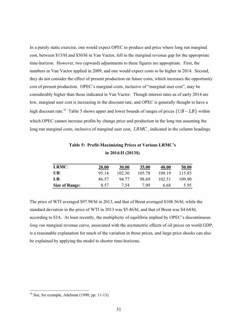
high discount rate.16 Table 5 shows upper and lower bounds of ranges of prices ( )UB LB− within

which OPEC cannot increase profits by change price and production in the long run assuming the

long run marginal costs, inclusive of marginal user cost, LRMC , indicated in the column headings.

Table 5: Profit-Maximizing Prices at Various LRMC’s

in 2014:II (2013$)

LRMC: 20.00 30.00 35.00 40.00 50.00UB: 95.14 102.30 105.78 109.19 115.85LB: 86.57 94.77 98.69 102.51 109.90Size of Range: 8.57 7.54 7.09 6.68 5.95

The price of WTI averaged $97.98/bl in 2013, and that of Brent averaged $108.56/bl, while the

standard deviation in the price of WTI in 2013 was $5.46/bl, and that of Brent was $4.64/bl,

according to EIA. At least recently, the multiplicity of equilibria implied by OPEC’s discontinuous

long run marginal revenue curve, associated with the asymmetric effects of oil prices on world GDP,

is a reasonable explanation for much of the variation in those prices, and large price shocks can also

be explained by applying the model to shorter time-horizons.

16 See, for example, Adelman (1990; pp. 11-13).

32

6 Conclusion

Instability in the price of crude oil does not imply that OPEC is unable to use its market power

effectively. The asymmetric effects of changes in the price of crude oil on the macroeconomy imply

that world demand and demand to OPEC net of non-OPEC production are kinked, that there is a

vertical discontinuity in OPEC’s marginal revenue curve. Therefore, there are multiple combinations

of price and OPEC production at which an increase in price (decrease in production) lowers revenue

more than cost, and at which a decrease in price (increase in production) raises revenue less than cost.

The asymmetry results in multiplicity of equilibria. In 2014, using long run demand, the range of

equilibrium prices appears to be about $7/bl wide, and an increase in price lasting one year to levels

above $142/bl would also appear to be profitable.

In the short run, demand to OPEC is quite inelastic, and the contemporaneous effects of changes in

price on GDP are negative and statistically significant. From Table 2, a 1% increase (decrease) in the

price of crude oil causes a 0.086% decrease (0.039% increase) in world GDP in the same quarter.

Assuming non-decreasing marginal costs, OPEC can collect a countercyclic stream of profits by

promulgating instability in the price of crude oil. The stream can be used to smooth out undesirable

fluctuations in consumption associated with the changes in GDP, so OPEC can sell instruments in

financial markets that command a risk premium. Thus, within some range, OPEC has incentive to

promulgate unstable prices for crude oil. Because increases in the price of crude oil damage the

macroeconomy more than decreases improve it, the instability in price that OPEC has incentive to

promulgate damages the macroeconomy.

The discontinuity in marginal revenue implies that vertical shifts in demand, associated with changes

in world GDP, cause larger changes in the price of crude oil. These, in turn, affect GDP.

33

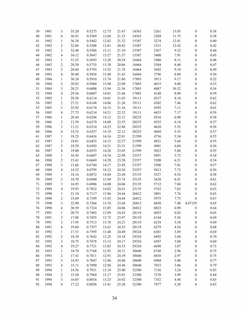
Table1: Basic Data A B C D E F G H I

Obs Year Qrtr Price

Implicit Price

Deflator

Non-OPEC Output

World Output

Annual World

GDP (PPP)

Quarterly U.S. GDP

Nominal Rate on 3-

Month Treasuries

Drop in World

Supply

Trade-Weighted ExchangeValue of

U.S.$

US$/bl 2005:I=1 bbl/yr bbl/yr bUS$ bUS$ secondary % 2005:I=1 1 1972 1 3.44 0 2 1972 2 3.77 0 3 1972 3 4.22 0 4 1972 4 4.86 0 5 1973 1 9.34 21.33 5988 1381 5.70 0 0.306 1973 2 9.58 21.79 5988 1418 6.60 0 0.297 1973 3 1.93 0.2837 9.68 22.28 5988 1437 8.32 0 0.288 1973 4 6.51 0.2893 9.64 21.19 5988 1479 7.50 4.90064 0.299 1974 1 12.94 0.2949 9.59 21.79 6697 1495 7.62 0 0.30

10 1974 2 12.66 0.3019 9.73 22.34 6697 1534 8.15 0 0.2911 1974 3 11.99 0.3109 9.69 21.38 6697 1563 8.19 0 0.3012 1974 4 13.64 0.3202 9.76 21.19 6697 1603 7.36 0 0.3013 1975 1 14.39 0.3276 9.73 20.23 7452 1620 5.75 0 0.3014 1975 2 13.29 0.3325 9.77 20.26 7452 1656 5.39 0 0.3015 1975 3 13.44 0.3386 10.11 21.55 7452 1714 6.33 0 0.3116 1975 4 15.88 0.3446 10.08 20.46 7452 1766 5.63 0 0.3217 1976 1 14.70 0.3484 10.12 21.26 8266 1825 4.92 0 0.3218 1976 2 13.16 0.3521 10.27 21.79 8266 1857 5.16 0 0.3319 1976 3 12.86 0.3569 10.48 22.51 8266 1891 5.15 0 0.3320 1976 4 14.64 0.3633 10.56 23.67 8266 1938 4.67 0 0.3321 1977 1 15.74 0.3694 10.77 23.20 9176 1993 4.63 0 0.3422 1977 2 14.27 0.3747 10.98 23.17 9176 2060 4.84 0 0.3423 1977 3 13.88 0.3793 11.12 22.95 9176 2122 5.50 0 0.3424 1977 4 15.69 0.3876 11.29 23.62 9176 2169 6.11 0 0.3325 1978 1 15.85 0.3933 11.39 22.59 10273 2209 6.39 0 0.3326 1978 2 14.21 0.4005 11.75 23.28 10273 2337 6.48 0 0.3327 1978 3 13.83 0.4072 11.81 23.69 10273 2399 7.31 0 0.3128 1978 4 15.82 0.4158 11.94 24.21 10273 2482 8.57 0 0.3129 1979 1 17.28 0.4232 11.99 23.74 11539 2532 9.38 1.9533 0.3230 1979 2 18.93 0.4336 12.16 24.64 11539 2596 9.38 0 0.3231 1979 3 23.38 0.4430 12.28 24.73 11539 2670 9.67 0 0.3232 1979 4 28.04 0.4519 12.39 24.68 11539 2731 11.84 0 0.3333 1980 1 33.54 0.4614 12.42 24.44 12875 2797 13.35 0 0.3334 1980 2 33.85 0.4718 12.52 23.68 12875 2800 9.62 0 0.3335 1980 3 33.81 0.4826 12.59 23.18 12875 2860 9.15 0 0.3336 1980 4 36.16 0.4959 12.51 22.12 12875 2994 13.61 4.54801 0.3337 1981 1 40.07 0.5085 12.71 23.03 14363 3132 14.39 0 0.3538 1981 2 37.49 0.5181 12.85 22.64 14363 3167 14.91 0 0.37

34

39 1981 3 35.28 0.5273 12.75 21.47 14363 3261 15.05 0 0.3840 1981 4 36.91 0.5369 12.68 21.33 14363 3284 11.75 0 0.3841 1982 1 36.38 0.5442 12.82 21.32 15387 3274 12.81 0 0.4042 1982 2 32.86 0.5508 13.01 20.82 15387 3331 12.42 0 0.4243 1982 3 32.48 0.5586 13.11 21.10 15387 3367 9.32 0 0.4444 1982 4 34.12 0.5647 13.27 21.57 15387 3408 7.91 0 0.4545 1983 1 31.55 0.5693 13.28 20.34 16464 3480 8.11 0 0.4646 1983 2 28.30 0.5735 13.39 20.86 16464 3584 8.40 0 0.4747 1983 3 28.60 0.5793 13.52 21.76 16464 3692 9.14 0 0.4948 1983 4 30.40 0.5836 13.48 21.63 16464 3796 8.80 0 0.5049 1984 1 30.24 0.5910 13.74 21.86 17883 3913 9.17 0 0.5250 1984 2 28.92 0.5960 13.90 22.09 17883 4015 9.80 0 0.5351 1984 3 28.21 0.6008 13.94 21.56 17883 4087 10.32 0 0.5652 1984 4 29.56 0.6047 14.01 21.46 17883 4148 8.80 0 0.5953 1985 1 28.58 0.6114 14.01 21.65 19111 4237 8.18 0 0.6254 1985 2 27.21 0.6148 14.06 21.26 19111 4302 7.46 0 0.6255 1985 3 25.92 0.6174 14.15 21.16 19111 4395 7.11 0 0.6156 1985 4 27.75 0.6214 14.21 22.32 19111 4453 7.17 0 0.5957 1986 1 20.44 0.6246 14.12 22.12 20235 4516 6.90 0 0.5858 1986 2 12.59 0.6279 14.09 22.55 20235 4555 6.14 0 0.5759 1986 3 11.21 0.6314 14.23 22.86 20235 4620 5.52 0 0.5660 1986 4 14.52 0.6357 14.19 22.12 20235 4669 5.35 0 0.5761 1987 1 18.25 0.6416 14.16 22.01 21599 4736 5.54 0 0.5562 1987 2 18.01 0.6453 14.15 22.27 21599 4821 5.66 0 0.5563 1987 3 18.39 0.6503 14.31 23.31 21599 4901 6.04 0 0.5664 1987 4 19.00 0.6553 14.26 23.05 21599 5023 5.86 0 0.5565 1988 1 16.56 0.6607 14.34 22.98 23357 5091 5.72 0 0.5466 1988 2 15.41 0.6669 14.28 23.20 23357 5208 6.21 0 0.5467 1988 3 13.66 0.6744 14.17 23.45 23357 5300 7.01 0 0.5768 1988 4 14.32 0.6795 14.12 24.36 23357 5413 7.73 0 0.5669 1989 1 18.16 0.6872 14.04 23.44 25135 5527 8.54 0 0.5870 1989 2 18.70 0.6940 13.94 23.74 25135 5628 8.41 0 0.6171 1989 3 16.95 0.6986 14.08 24.06 25135 5712 7.84 0 0.6272 1989 4 19.93 0.7032 14.02 24.41 25135 5763 7.65 0 0.6373 1990 1 21.10 0.7117 13.96 24.64 26812 5891 7.76 0 0.6574 1990 2 15.69 0.7199 13.92 24.64 26812 5975 7.75 0 0.6775 1990 3 22.90 0.7266 13.76 23.64 26812 6030 7.48 4.07159 0.6576 1990 4 30.59 0.7324 13.85 24.06 26812 6023 6.99 0 0.6477 1991 1 20.75 0.7403 13.99 24.43 28119 6055 6.02 0 0.6578 1991 2 17.88 0.7455 13.73 23.97 28119 6144 5.56 0 0.6979 1991 3 17.95 0.7513 13.70 24.21 28119 6218 5.38 0 0.6980 1991 4 19.84 0.7557 13.63 24.33 28119 6279 4.54 0 0.6881 1992 1 17.51 0.7595 13.40 24.49 29324 6381 3.89 0 0.6982 1992 2 18.39 0.7642 13.25 24.18 29324 6492 3.68 0 0.7083 1992 3 18.75 0.7678 13.13 24.17 29324 6587 3.08 0 0.6984 1992 4 19.27 0.7721 13.03 24.35 29324 6698 3.07 0 0.7385 1993 1 18.70 0.7768 12.93 24.71 30640 6748 2.96 0 0.7586 1993 2 17.41 0.7811 12.91 24.39 30640 6830 2.97 0 0.7587 1993 3 14.93 0.7847 12.86 24.40 30640 6904 3.00 0 0.7788 1993 4 15.11 0.7890 12.96 24.46 30640 7033 3.06 0 0.7989 1994 1 14.36 0.7931 13.14 25.00 32380 7136 3.24 0 0.8390 1994 2 15.50 0.7969 13.17 25.03 32380 7270 3.99 0 0.8491 1994 3 16.03 0.8016 13.23 24.92 32380 7352 4.48 0 0.8392 1994 4 17.22 0.8058 13.41 25.20 32380 7477 5.28 0 0.83

35

93 1995 1 18.35 0.8104 13.39 25.48 34186 7545 5.74 0 0.8594 1995 2 17.96 0.8140 13.38 25.66 34186 7605 5.60 0 0.8295 1995 3 15.92 0.8178 13.58 25.77 34186 7707 5.37 0 0.8496 1995 4 17.83 0.8220 13.53 25.69 34186 7800 5.26 0 0.8697 1996 1 19.74 0.8267 13.67 26.14 36226 7893 4.93 0 0.8898 1996 2 19.99 0.8299 13.76 26.24 36226 8062 5.02 0 0.8999 1996 3 20.06 0.8325 13.79 26.18 36226 8159 5.10 0 0.89

100 1996 4 24.08 0.8371 13.93 26.44 36226 8287 4.98 0 0.90101 1997 1 22.37 0.8425 14.00 26.95 38351 8402 5.06 0 0.93102 1997 2 17.64 0.8445 14.01 27.03 38351 8552 5.05 0 0.94103 1997 3 17.10 0.8474 14.03 27.06 38351 8692 5.05 0 0.96104 1997 4 18.57 0.8506 14.13 27.25 38351 8788 5.09 0 0.99105 1998 1 14.68 0.8520 14.19 28.01 39790 8890 5.05 0 1.05106 1998 2 12.07 0.8540 14.15 27.90 39790 8995 4.98 0 1.05107 1998 3 11.22 0.8573 14.01 27.29 39790 9147 4.82 0 1.08108 1998 4 11.88 0.8599 14.03 27.26 39790 9326 4.25 0 1.05109 1999 1 12.22 0.8637 14.12 27.82 41827 9450 4.41 0 1.06110 1999 2 15.16 0.8668 13.99 27.09 41827 9562 4.45 0 1.07111 1999 3 19.09 0.8700 14.14 27.23 41827 9719 4.65 0 1.06112 1999 4 24.08 0.8731 14.27 27.14 41827 9932 5.04 0 1.05113 2000 1 28.15 0.8800 14.30 27.74 44729 10036 5.52 0 1.06114 2000 2 26.25 0.8845 14.33 28.33 44729 10284 5.71 0 1.08115 2000 3 28.46 0.8898 14.48 28.69 44729 10364 6.02 0 1.10116 2000 4 29.35 0.8945 14.57 28.79 44729 10475 6.02 0 1.13117 2001 1 25.51 0.9005 14.54 28.80 46866 10513 4.82 0 1.13118 2001 2 23.59 0.9067 14.42 28.23 46866 10642 3.66 0 1.16119 2001 3 22.35 0.9095 14.62 28.34 46866 10644 3.17 0 1.15120 2001 4 17.97 0.9123 14.70 28.06 46866 10703 1.91 0 1.16121 2002 1 20.54 0.9156 14.76 27.99 49015 10837 1.72 0 1.18122 2002 2 23.69 0.9197 14.95 27.98 49015 10938 1.72 0.05313 1.16123 2002 3 25.27 0.9236 14.86 28.06 49015 11040 1.64 0 1.14124 2002 4 26.50 0.9289 14.90 28.38 49015 11106 1.33 0 1.15125 2003 1 31.94 0.9354 15.00 28.89 51824 11231 1.16 0 1.13126 2003 2 25.35 0.9382 14.98 28.80 51824 11371 1.04 0.3079 1.09127 2003 3 26.71 0.9434 15.16 28.91 51824 11628 0.93 0 1.09128 2003 4 28.85 0.9482 15.32 29.60 51824 11819 0.92 0 1.06129 2004 1 32.34 0.9564 15.30 30.07 55655 11991 0.92 0 1.03130 2004 2 33.55 0.9645 15.41 30.27 55655 12184 1.08 0 1.06131 2004 3 37.93 0.9715 15.34 30.52 55655 12369 1.49 0 1.05132 2004 4 40.82 0.9787 15.31 30.48 55655 12564 2.01 0 1.01133 2005 1 42.36 0.9878 15.26 30.81 59560 12816 2.54 0 1.00134 2005 2 45.64 0.9944 15.45 31.16 59560 12976 2.86 0 1.01135 2005 3 56.09 1.0046 15.14 30.81 59560 13207 3.36 0 1.01136 2005 4 53.09 1.0130 15.16 30.72 59560 13383 3.83 0 1.02137 2006 1 56.01 1.0206 15.22 30.99 63420 13650 4.39 0 1.01138 2006 2 63.26 1.0295 15.22 30.93 63420 13803 4.70 0 0.99139 2006 3 63.25 1.0372 15.27 30.99 63420 13911 4.91 0 0.99140 2006 4 54.50 1.0419 15.28 30.69 63420 14068 4.90 0 0.98141 2007 1 54.57 1.0538 15.30 30.87 68710 14235 4.98 0 0.98142 2007 2 62.14 1.0610 15.29 30.91 68710 14425 4.74 0 0.96143 2007 3 69.79 1.0645 15.16 30.73 68710 14572 4.30 0 0.94144 2007 4 83.50 1.0696 15.10 30.94 68710 14690 3.39 0 0.91145 2008 1 91.08 1.0759 15.08 31.42 72112 14673 2.04 0 0.89146 2008 2 115.56 1.0830 15.06 31.44 72112 14817 1.63 0 0.88

36

147 2008 3 111.12 1.0916 14.86 31.16 72112 14844 1.49 0 0.89148 2008 4 52.89 1.0930 14.95 30.82 72112 14547 0.30 0 0.99149 2009 1 41.81 1.0972 15.08 30.65 72119 14381 0.21 0 1.01150 2009 2 57.30 1.0959 15.10 30.75 72119 14342 0.17 0 0.98151 2009 3 65.74 1.0966 15.22 30.88 72119 14384 0.16 0 0.95152 2009 4 74.09 1.0994 15.29 30.92 72119 14564 0.06 0 0.92153 2010 1 76.54 1.1036 15.38 31.22 76810 14673 0.11 0 0.93154 2010 2 74.09 1.1079 15.41 31.46 76810 14879 0.15 0 0.95155 2010 3 72.65 1.1116 15.40 31.46 76810 15050 0.16 0 0.93156 2010 4 81.94 1.1164 15.48 31.43 76810 15232 0.14 0 0.91157 2011 1 95.42 1.1240 15.45 30.35 81330 15243 0.13 3.43509 0.89158 2011 2 108.55 1.1312 15.30 29.95 81330 15462 0.05 1.3259 0.87

A: refiners' acquisition cost of imported crude oil, U.S. dollars per barrel; 1973:III is official price of Saudi Light; from U.S. Energy Information Administration B: U.S. gross domestic product implicit price deflator; quarterly figures from Federal Reserve Bank of St. Louis http://research.stlouisfed.org/fred2/data/GDPDEF.txt, accessed April 1, 2014. C: non-OPEC production of crude oil; from U.S. Energy Information Administration, http://www.eia.doe.gov/emeu/international/oilproduction.html, accessed April 1, 2014. D: world crude oil production; from U.S. Energy Information Administration, also http://www.eia.doe.gov/emeu/international/oilproduction.html, accessed April 1, 2014. E: world gross domestic product; from IMF World Economic Outlook, April 2005, http://www.imf.org/external/pubs/ft/weo/2005/01/data/dbasubm.cfm and IMF World Economic Outlook, April 2009, http://www.imf.org/external/pubs/ft/weo/2009/01/weodata/weoselser.aspx?a=1&c=001&t=1

F: quarterly U.S. gross domestic product; from Federal Reserve Bank of St. Louis http://research.stlouisfed.org/fred2/data/GDP.txt, accessed April 1, 2014.

G: nominal rate on 3-Month U.S. treasury securities, secondary market; from http://www.federalreserve.gov/releases/H15/data/Monthly/H15_TB_M3.txt H: percent drop in world output due to violence; from EIA Monthly Energy Review http://www.eia.doe.gov/emeu/international/oilproduction.html, accessed April 1, 2014. I: Trade-Weighted Exchange Value of U.S. Dollar; from Federal Reserve Bank of Saint Louis http://research.stlouisfed.org/fred2/data/TWEXBMTH.txt, accessed April 1, 2014.

37

REFERENCES Adelman, M.A., 1990. OPEC at thirty years: what have we learned? Annual Review of Energy 15, 1-22. Adelman, M.A., 2004. The real oil problem. Regulation, Spring 2004, 16-21. Angus Maddison Project, http://www.ggdc.net/maddison/maddison-project/home.htm, accessed April 3, 2014. Atkins, F.J., Jazayeri, S.M.T., 2004. A Literature Review of Demand Studies in World Oil Markets. University of Calgary, Discussion Paper 2004-07. Bible, The, Young’s Literal Translation of, 1898, 3rd ed. Greater Truth Publishers, 2004, Lafayette, IN. Cashin, Paul and C. John McDermott, 2001. An Unbiased Appraisal of Purchasing Power Parity. IMF working paper WP/01/196. Celta, D.J., Dahl, C.A., 2000. OPEC as a social welfare maximizer. Colorado School of Mines working paper, February. Cumby, R. E., and J. Huizinga. 1992. Testing the autocorrelation structure of disturbances in ordinary least squares and instrumental variables regressions. Econometrica 60(1): 185–195. Djankov, Simeon and Marta Reynal-Querol, 2007. The Causes of Civil War. Working Paper available at http://www.doingbusiness.org/documents/causes_of_civil_wars.pdf. Energy Information Administration, U.S. Department of Energy, http://www.eia.gov/ Evans, William N., and Robert M. Schwab, 1995. Finishing High School and Starting College: Do Catholic Schools Make a Difference? Quarterly Journal of Economics, 110, 947-974. Federal Reserve Bank of St. Louis, http://research.stlouisfed.org/fred2/series/OILPRICE/downloaddata?cid=98. Frasco, Gregg P., 1993. The Kinked Demand Curve When Demand Shifts. Journal of Economic Education 24:2, 137-143. Gately, Dermot and Hillard G. Huntington, 2002. The Asymmetric Effects of Changes in Price and Income on Energy and Oil Demand, Energy Journal 23:1, 19-55. Greene, David L. and Sanjana Ahmad, 2005. Costs of U.S. Oil Dependence: 2005 Update. Oak Ridge National Laboratory, U.S. Dept. of Energy. ORNL/TM-2005/45. Greenhouse, Steven, 1987. When the World’s Growth Slows. New York Times, December 27.

38

Griffin, J.M., Schulman, C.T., 2005. Price asymmetry in energy demand models: a proxy for energy-saving technical change? Energy Journal 26, 1-21. Hamilton, James D., 2003. What is an oil shock? Journal of Econometrics 113, 363-398. Hamilton, James D., 2009. Causes and Consequences of the Oil Shock of 2007-08, Brookings Papers on Economic Activity, Spring 2009 Conference Draft. Moran, Theodore H., January 1993. Managing an oligopoly of would-be sovereigns: the dynamics of joint control and self-control in the international oil industry past, present, and future. In The International Political Economy of Natural Resources (Vol 1), Mark Zacher, ed. Edward Elgar Publishing, Brookfield, VT. Organization of Petroleum Exporting Countries (OPEC), http://www.opec.org/home/ Robinson, P.M., 1995. Log-periodogram regression of time series with long range dependence. Annals of Statistics 23, 1048-1072. Shepherd, Geoffrey, 1933. Vertical and Horizontal Shifts in Demand Curves. Journal of Farm Economics 15:4, 723-729. Stevens, P., 2005. Oil markets. Oxford Review of Economic Policy 21:1, 19-42. Teitenberg, Tom, 2007. Environmental Economics and Policy. 5th ed. Pearson Addison-Wesley. Van Vactor, S.A., 2010. Introduction to the Global Oil and Gas Business. Penn Well Corporation, Tulsa, OK. Verleger, P.K., 2005. Are oil markets entering yet another “new era”? The Petroleum Economics Monthly 22:7. Wing, I.S., 2008. Explaining the declining energy intensity of the U.S. economy. Resource and Energy Economics 30, 21-49. Wooldridge, Jeffrey M., 2002. Econometric Analysis of Cross Section and Panel Data. MIT Press, Cambridge, MA.