OPAC103

GEOMETRICAL OPTICS

LABORATORY MANUAL

Gaziantep University

Department of Optical & Acoustical Engineering opac.gantep.edu.tr

Dr. Ahmet Bingül

Oct 2018

Some parts of this manual are extracted from www.pasco.com.

2

3

Content*

Title Brief Description Page

Laboratory Equipment

Optics and Opto-mechanics used in Laboratory 2

Preface

Of this Manual 4

Experiment 1

Color Addition 5

Experiment 2

Inverse Square Law 6

Experiment 3

Shadows 9

Experiment 4

Snell’s Law of Refraction 12

Experiment 5

Total Internal Reflection 15

Experiment 6

Optical Slab 18

Experiment 7

Minimum Angle of Deviation of a Prism 20

Experiment 8

Focal Length and Magnification of Concave Mirror 23

Experiment 9

Focal Length and Magnification of Thin Lens 26

Experiment 10

Lens Maker’s Equation 29

Experiment 11

Telescope and Microscope 31

Appendix A

Experimental Errors 37

Appendix B

Basic Gnuplot Commands

40

Appendix C

An Example Report

48

* Performing the experiments depend on the duration of semester.

4

Preface

This is the laboratory manual for the first year lab course named Geometric Optics Laboratory in

Optical & Acoustical Engineering Department at Gaziantep University. These notes are compiled after

experiences of 3 years in the Optics Laboratory in the department.

This manual includes 11 experiments (for one semester) based on the approximation called

geometrical optics. The students will understand and validate the basic principles of the geometrical optics.

We shall also discuss some elementary applications to a number of practical devices in the lab. It is strongly

suggested that the students and Lab assistants should read the manual carefully before performing the

experiments.

At the end of each experiment, student groups must prepare a report (2-3 pages) within one week and

present it to the Lab Assistant. Note that an example written report is given in Appendix.

Ahmet Bingül

Oct, 2017

5

EXPERIMENT 1

COLOR ADDITION

PURPOSE

You will discover the results of mixing red, green, and blue light in different combinations.

EQUIPMENT

Light Source Convex Lens from Ray Optics Kit

Other Required Equipment PROCEDURE

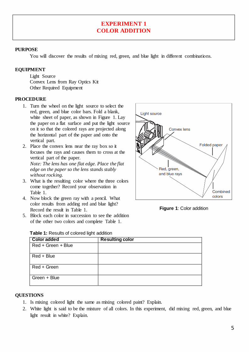
1. Turn the wheel on the light source to select the red, green, and blue color bars. Fold a blank, white sheet of paper, as shown in Figure 1. Lay

the paper on a flat surface and put the light source on it so that the colored rays are projected along

the horizontal part of the paper and onto the vertical part.

2. Place the convex lens near the ray box so it

focuses the rays and causes them to cross at the vertical part of the paper.

Note: The lens has one flat edge. Place the flat edge on the paper so the lens stands stably without rocking.

3. What is the resulting color where the three colors come together? Record your observation in

Table 1. 4. Now block the green ray with a pencil. What

color results from adding red and blue light?

Record the result in Table 1. 5. Block each color in succession to see the addition

of the other two colors and complete Table 1.

Figure 1: Color addition

Table 1: Results of colored light addition

Color added Resulting color

Red + Green + Blue

Red + Blue

Red + Green

Green + Blue

QUESTIONS

1. Is mixing colored light the same as mixing colored paint? Explain.

2. White light is said to be the mixture of all colors. In this experiment, did mixing red, green, and blue

light result in white? Explain.

6

EXPERIMENT 2

INVERSE SQUARE LAW

PURPOSE

To verify inverse square law using point-like light source.

EQUIPMENT

Point-like light source (Tungsten Lamb) Luxmeter

Optical bench THEORY

In optics, inverse-square law states that the intensity (irradiance or illumination) of a point light source is inversely proportional to the square of the distance from the source. This is due to geometric dilution

corresponding to point-source radiation into three-dimensional space (see Figure 1). That is:

The intensity of a light source has SI unit W/m2 = J/(s.m2). Namely, the intensity is the light energy falling on unit area per unit time. Let the total power radiated from a point source be P. This light power is distributed over the spherical surface as the distance from the source increases. Since the surface area of a

sphere of radius r is A = 4πr2, then intensity I (power per unit area) of radiation at distance r is

(1)

where k = P/4π is a constant. Therefore, the intensity is inversely proportional to square of the distance. In physics, there are many other phenomena which can be explained by means of the inverse square law

such as Newton's law of universal gravitation, electric field, magnetic field, sound, and radiation.

Figure 1: The inverse square law

7

Optical Measurement

In optics, the electromagnetic radiation measurement is studied in two groups:

1. radiometry is the measurement of optical radiation including visible light 2. photometry is the measurement of visible light only

The light power and intensity can be expressed in radiometric and photometric units. Table 1 shows the conversion between radiometric and photometric units.

Table 1: Basic Radiometric and Photometric units

Quantity Radiometric unit Photometric unit Conversion

Power P (in Watts, W) Φ (in lumens, lm) Φ = 683 P(λ) V(λ)

Intensity I (in W/m2) E (in lm/m

2 = lux) E = 683 I(λ) V(λ)

Here V(λ) is a function of wavelength, λ. Its form can be found in many text books.

Figure 2 shows a simple luxmeter which is an instrument for measuring light intensity in photometric unit,

illuminance (E).

Figure 2: Luxmeter is used for measuring illumination.

PROCEDURE

The setup of the experiment as shown in Figure 3 where x represents the distance between point-like source

and luxmeter.

1. Place the light source at the position 0.0 cm on the optical bench. 2. Turn off most of the room lights. We want the relativity intensity levels to not vary by more than 1-2

percent as the luxmeter is moved down the track. You should keep your hand and body behind

luxmeter to avoid reflecting light onto it. 3. Start measuring illuminance with the luxmeter x = 20 cm from the center of the light source.

4. Repeat the measurements for the luxmeter positions [30 cm, 40 cm, … , 100 cm] from the source. 5. Record your results in Table 2.

Figure 3: The setup

8

Table 2: The experimental data

Distance from the source x, (m)

Measured illumination, E (lux)

0.2 0.3 0.4 0.5 0.6 0.7 0.8 0.9 1.0

Table 3: Fitting procedure

Fit Equation 1 Fit Equation 2 Fit Equation 3

a = n =

a = b = n =

a = b = c = n =

Goodness of the fit:

Goodness of the fit:

Goodness of the fit:

QUESTIONS

1. The intensity on the Earth (just above the atmosphere) is about 1350 W/m2 due to Sun. What is the power of the Sun? What is the intensity on Mercury and on Mars?

2. Plot E versus x graph. Fit the data points in the Table 2 to the functions in Table 3 to find the

coefficients a, b, c and n. 3. Record the values of fitting parameters, their associated errors and goodness of each fit in Table 3.

4. Explain the physical meaning of these fitting coefficients, a, b, c and n. 5. Normally it is expected that n = 2.0. For each fitting function, calculate percentage difference

between the expected value and the fitting value.

6. The fitting function (say first one) can be used to estimate the light intensity at any point from the source. What is the illuminance at x = 1.5 m?

7. What is your conclusion?

9

EXPERIMENT 3

SHADOWS AND RAY MODEL OF LIGHT

PURPOSE

To obtain relations between the object size and its shadow size as a function of distance.

EQUIPMENT

Point-like Light source (Tungsten Lamb) Screen, Ruler

Circular opaque object

THEORY

Shadows are produced on a screen behind the object when the light from a source is blocked (either

completely or only partially) by the object. In the case where geometrical optics is appropriate, the shadow

can be constructed using simple straight-line rays and the simple geometry, Figure 1.

Figure 1: Shadow of an object

A clear unambiguous shadow requires a “point” source of light – something that either is very small

compared to the other dimensions of the experiment or else is very far away. The geometrical construction

of the shadow is particularly simple in this case, since all of the rays that strike the object come from a single

point, so that a given point of the image either receives light or doesn’t.

If the source of light is too large to be regarded as a “point” source, then the shadow is constructed using the

principle of superposition – the extended source is modeled as a large number of point sources, and the

shadow produced by each of these point sources is constructed independently. In this case you will see two

types of shadows, Figure 2. The umbra: the portion of the shadow which is totally dark because light from

all sources is absent and The penumbra: the portion of the shadow which is illuminated by some of the

sources and is therefore not completely dark.

Figure 2: The umbra and the penumbra effects observed during the Solar Eclipse.

10

PROCEDURE

The setup of the experiment is shown in Figure 3 where x represents the distance between point-like source

and circular opaque object (Figure 4) which can be obtained from the PASCO Basic Optics System.

1. Keep the distance between the source and the screen constant at d = 800 mm.

2. Change the distance x for the values in the Table 1.

3. Measure the diameter (D) of the object’s shadow by using cheap ruler. Record the result in Table 1.

4. Calculate the theoretical (expected) diameter of the object’s shadow. Record the result in Table 1.

5. Finally compute the percentage error between the results in case 4 and 5.

Figure 3: The setup for the experiment

Figure 4: Circular opaque object and its shadow

11

Table 1: The experimental data

Original diameter of the circular opaque object in mm, Do =

Distance between the

source and circular

object (x) in mm

Measured diameter (D)

of the object’s shadow

in mm

Expected diameter (D)

of the object’s shadow

in mm

% Error

150 200 250 300 350 400 450 500 550 600 650 700

QUESTIONS

1. What are the physical and the geometrical principles behind this experiment?

2. Compute the solid angles of Moon and Sun subtended from Earth and explain the solar eclipse.

3. Plot x vs “measured D” graph.

4. Plot x vs “measured 1/D” graph and fit your data to a linear function to obtain value of the original

diameter (Do) of the opaque object. Compare your results with the value in the Table 1.

5. What is your overall conclusion?

12

EXPERIMENT 4

SNELL’S LAW OF REFRACTION

PURPOSE

The aim of the experiment is to measure index of refraction of a material using Snell’s law.

EQUIPMENT

Laser source Angular indicator

D-shaped transparent material

THEORY

When a ray of light is refracted at an interface dividing two transparent media, the transmitted ray remains

within the plane of incidence and the sine of the angle of refraction θ 2 is directly proportional to the sine of

the angle of incidence θ1, Figure 1. Including wavelengths (λ), phase velocities (v) and index of refraction

(n), the mathematical form of the Snell’s law is as follows:

(1)

Figure 1: Refraction of light at the interface between two media of different refractive indices, with n1 < n2. Since the

velocity is lower in the second medium (v2 < v1), the angle of refraction θ2 is less than that of the angle of incidence θ1;

that is, the ray in the higher-index medium is closer to the normal.

13

PROCEDURE

1. Place D-shaped plastic optical material on the angular indicator as shown in Figure 2.

2. Turn on the laser source. Allow the laser beam to fall on the center of the D-shaped material as indicated in Figure 2.

3. Change the angle of incidence (θ1) and measure angle of refraction (θ2). 4. Compute sin(θ1), sin(θ2) and index of refraction n for each angle. (Record the result in Table 1)

Figure 2: The setup to verify the Snell’s law. Incidence and reflection angle are 60

o and

refraction angle is about 35o with respect to normal corresponding to 0

o.

Table 1: The experimental data

Angle of incidence θ1 (in degrees)

Angle of refraction

θ2 (in degrees)

sin(θ1) sin(θ2) index of refraction

n

5

10

15

20

25

30

35

40

45

50

55

60

65

70

Average, <n> =

Standard Deviation, σ =

Standard Error, σE =

14

QUESTIONS

1. Explain the advantage of using D-shaped material in the experiment. 2. Calculate the mean value of the index of refraction, its standard deviation and standard error.

3. Plot sin(θ2) [in x-axis] vs sin(θ1) [in y-axis] graph and obtain the value of n from the linear fit (See Appendix related to Fitting).

4. What is your conclusion?

15

EXPERIMENT 5

TOTAL INTERNAL REFLECTION

PURPOSE

The aim of the experiment is to measure refractive index of a transparent material using critical angle

EQUIPMENT

Laser source, Angular indicator, D-shaped transparent material and prism.

THEORY

Consider a light source at point S as shown in Figure 1. Rays from the source that make increasingly larger

angles of incidence with the interface must refract at increasingly larger angles. A critical angle θc of

incidence is reached when the angle of refraction reaches 90°. Thus, from Snell’s law,

or

(1)

For angles of incidence θ1>θc the incident ray experiences total internal reflection (TIR) as shown.

Otherwise both refraction and reflection occur.

Notes:

TIR does not occur unless n1 > n2.

if n2 is air (that is n2 = 1) and n1 = n then θc = arcsin(1/n).

Figure 1 Refraction of light at the interface between two media of different refractive indices, with n1>n2.

16

PROCEDURE

Part 1: Use D-Shape

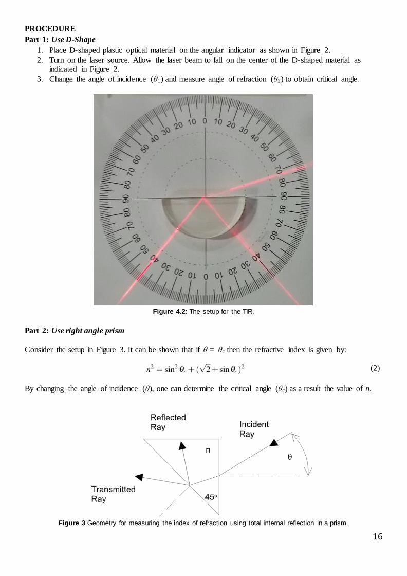
1. Place D-shaped plastic optical material on the angular indicator as shown in Figure 2.

2. Turn on the laser source. Allow the laser beam to fall on the center of the D-shaped material as indicated in Figure 2.

3. Change the angle of incidence (θ1) and measure angle of refraction (θ2) to obtain critical angle.

Figure 4.2: The setup for the TIR.

Part 2: Use right angle prism

Consider the setup in Figure 3. It can be shown that if θ = θc then the refractive index is given by: (2)

By changing the angle of incidence (θ), one can determine the critical angle (θc) as a result the value of n.

Figure 3 Geometry for measuring the index of refraction using total internal reflection in a prism.

17

QUESTIONS

1. Give two example applications of TIR in our daily life. 2. Derive Equation 2.

3. In part 1, assume that the any angle measurement has an uncertainty about ±0.5o. Using Equation 1 for n1 = n and n2 = 1, find the index of refraction of the material and its uncertainty. (See Appendix related to error calculations)

4. Calculate the percentage difference between the expected value of n = 1.5. 5. In part 2, determine the index of refraction and its associated error.

6. Calculate the percentage difference between the expected value of n = 1.5. 7. What is your conclusion?

18

EXPERIMENT 6

OPTICAL SLAB

PURPOSE

The aim of this experiment is to measure index of refraction of an optical slab.

EQUIPMENT

Laser source, Angular indicator, ruler and Optical slab

THEORY

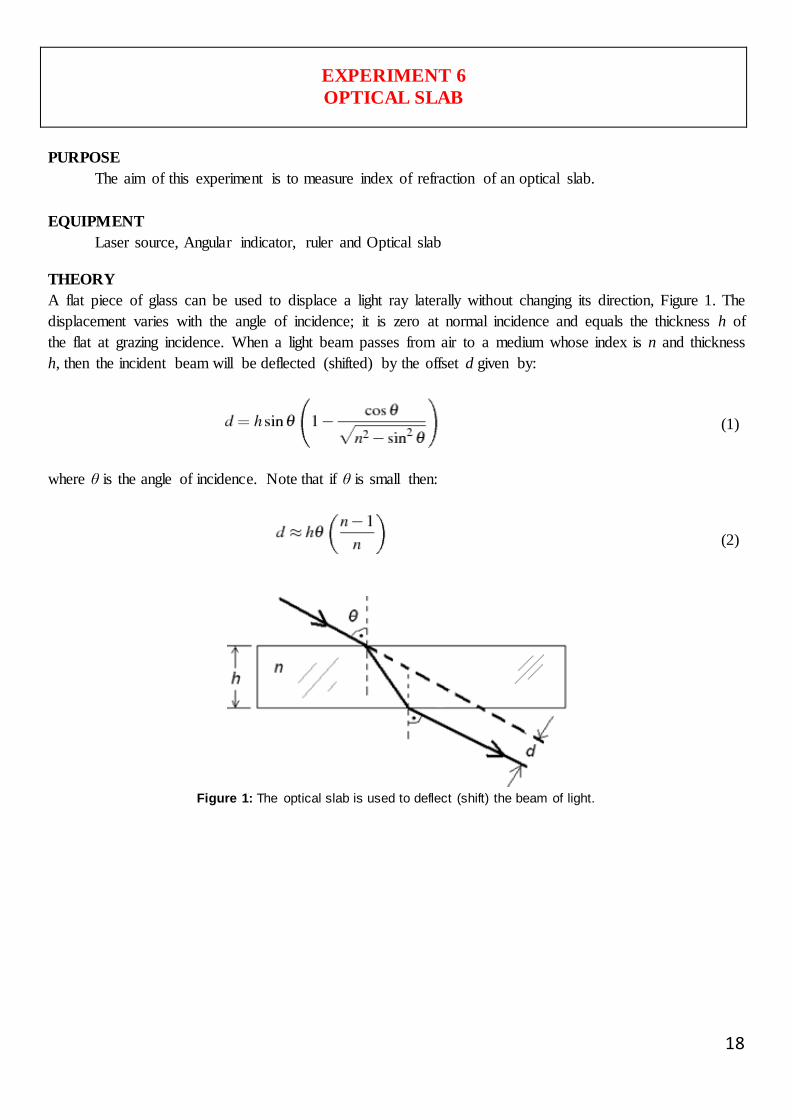
A flat piece of glass can be used to displace a light ray laterally without changing its direction, Figure 1. The

displacement varies with the angle of incidence; it is zero at normal incidence and equals the thickness h of

the flat at grazing incidence. When a light beam passes from air to a medium whose index is n and thickness

h, then the incident beam will be deflected (shifted) by the offset d given by:

(1)

where θ is the angle of incidence. Note that if θ is small then:

(2)

Figure 1: The optical slab is used to deflect (shift) the beam of light.

19

Figure 2: The setup for the optical slab

PROCEDURE

1. Place the optical slab whose thickness is h = 60 mm on the angular indicator as shown in Figure 2. 2. Turn on the laser source.

3. Determine the angle of incidence (θ) by measuring the angle of reflection. (How?) 4. Using ruler, measure the distance d for different angle of incidence and fill Table 1 below.

Table 1: The experimental data

Angle of incidence θ (deg)

Angle of incidence θ (rad)

Offset distance d (mm)

Index of refraction n

10 20 30 40 50 60 70

Average index of refraction, <n> = Standard Deviation, σ =

Standard Error, σE =

QUESTIONS

1. Derive Equation 1 and Equation 2. 2. Calculate mean value of the index of refraction and its standard deviation.

3. Plot θ vs d graph and obtain the value of index of refraction and its uncertainty by using the non-linear fitting method (see Appendix).

4. Find the percentage error between your results and accepted value (n = 1.5).

5. What is your conclusion?

20

EXPERIMENT 7

MINIMUM ANGLE OF DEVIATION OF A PRISIM

PURPOSE

In this experiment you will measure minimum deviation angle and index of refraction of a prism.

EQUIPMENT

Laser source, prism, milli-metric paper

THEORY

Consider typical dispersing prism in air as shown in Figure 1.

α1= angle of incidence

α2 = outgoing angle

A = apex angle

D = angle of deviation = α1 + α2–A

n = index of refraction

Figure 1: Typical dispersing prism

From geometry, the angle of deviation as a function of α1 and n is as follows:

(1)

Figure 2. D vs α1 for A=30o and n = 1.5.

An example graph of the angle of incidence vs angle of

deviation is shown in Figure 2. By minimizing Equation 1, one can prove that the

minimum angle of deviation (Dmin) and index of refraction (n) is related by the formula:

(2)

21

PROCEDURE

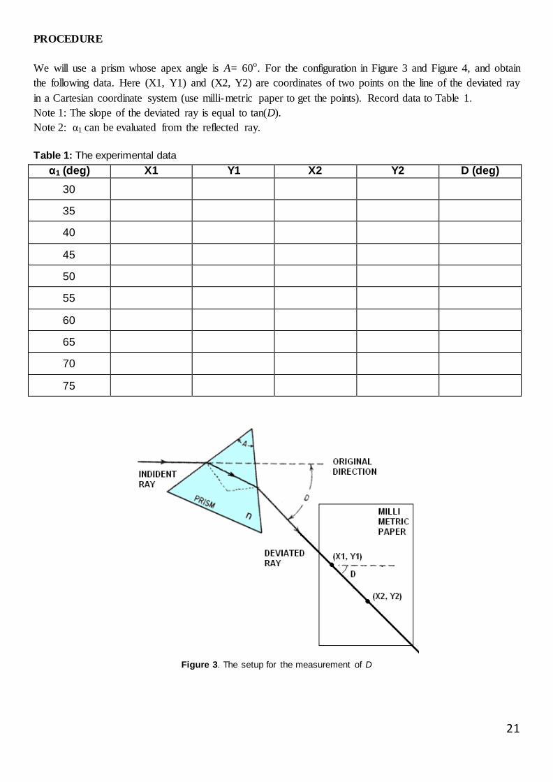
We will use a prism whose apex angle is A= 60o. For the configuration in Figure 3 and Figure 4, and obtain

the following data. Here (X1, Y1) and (X2, Y2) are coordinates of two points on the line of the deviated ray

in a Cartesian coordinate system (use milli-metric paper to get the points). Record data to Table 1.

Note 1: The slope of the deviated ray is equal to tan(D).

Note 2: α1 can be evaluated from the reflected ray.

Table 1: The experimental data

α1 (deg) X1 Y1 X2 Y2 D (deg)

30 35 40 45 50 55 60 65 70 75

Figure 3. The setup for the measurement of D

22

QUESTIONS

1. Derive Equation 1 and Equation 2.

2. Plot α1 vs D and fit your data to Equation 1 to find the value of n. (See Appendix).

3. Determine the Dmin from the final fit function and evaluate the value of n via Equation 2.

4. Compute the percentage error between your observations and the actual value of n = 1.5.

5. What is your overall conclusion?

Figure 4: Photograph taken from a real experiment.

23

EXPERIMENT 8

FOCAL LENGTH AND MAGNIFICATION OF CONCAVE MIRROR

PURPOSE

The purpose of this experiment is to determine the focal length of a concave mirror and to measure

the magnification for a certain combination of object and image distances.

EQUIPMENT

Light Source, Bench, Concave/convex Mirror, Half-screen, Metric ruler, Caliper

THEORY

For a spherically curved mirror, the mirror equation is given by:

(1)

where

f = focal length of mirror

do = distance between the object and the mirror

di = distance between the image and the mirror

By measuring do and di, the focal length can be determined. In paraxial region, the radius of curvature of the

mirror, R, and the focal length are related by:

(2)

Magnification, m, is the ratio of image size (hi) to object size (ho):

(3)

Alternatively, the magnification can be deduced from the object and image distances:

(4)

Note that the sign conventions are as follows:

Quantity Positive when Negative when

f Concave mirror is used Convex mirror is used R Concave mirror is used Concave mirror is used

do Object is real Object is not real di Image is real Image is not real

m Image is inverted Image is upright

24

PROCEDURE

You will determine the focal length of the mirror by measuring several pairs of object and image distances

and plotting 1/ do versus1/di graph.

1. Place the light source and the mirror on the optics bench 50 cm apart with the light source’s crossed-

arrow object toward the mirror and the concave side of the mirror toward the light source. Place the

half-screen between them (see Figure 1).

2. Slide the half-screen to a position where a clear image of the crossed-arrow object is formed.

Measure the image distance and the object distance, and image height and image height. Record

these measurements (and all measurements from the following steps) in Table 1. (You can measure

the object size directly from the light source. Δm is the difference between magnifications using

Equations 3 and 4).

3. Repeat step 2 with object distances of 45 cm, 40 cm, 35 cm, 30 cm, 25 cm.

Figure 1: The setup

Figure 2: Example image on the half screen

25

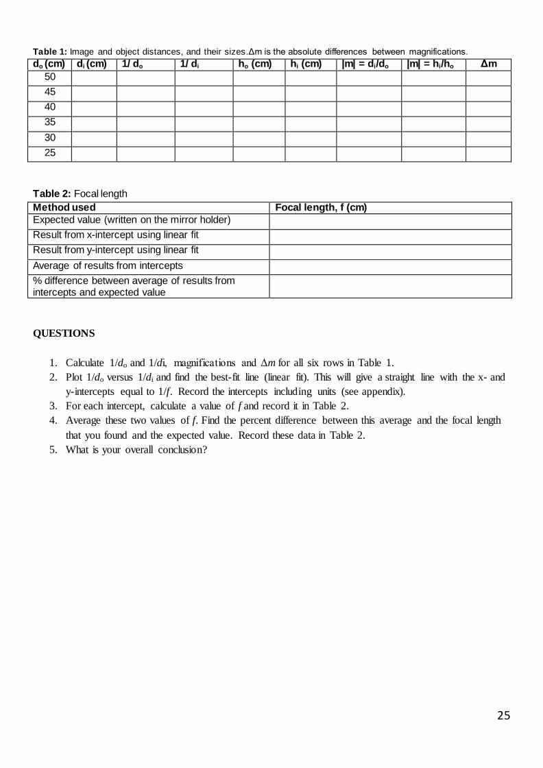
Table 1: Image and object distances, and their sizes.Δm is the absolute differences between magnifications.

do (cm) di (cm) 1/ do 1/ di ho (cm) hi (cm) |m| = di/do |m| = hi/ho Δm

50 45 40 35 30 25

Table 2: Focal length

Method used Focal length, f (cm)

Expected value (written on the mirror holder) Result from x-intercept using linear fit Result from y-intercept using linear fit Average of results from intercepts % difference between average of results from intercepts and expected value

QUESTIONS

1. Calculate 1/do and 1/di, magnifications and Δm for all six rows in Table 1.

2. Plot 1/do versus 1/di and find the best-fit line (linear fit). This will give a straight line with the x- and

y-intercepts equal to 1/f. Record the intercepts including units (see appendix).

3. For each intercept, calculate a value of f and record it in Table 2.

4. Average these two values of f. Find the percent difference between this average and the focal length

that you found and the expected value. Record these data in Table 2.

5. What is your overall conclusion?

26

EXPERIMENT 9

FOCAL LENGTH AND MAGNIFICATION OF THIN LENS

PURPOSE

The purpose of this experiment is to determine the focal length of a thin lens and to measure the

magnification for a certain combination of object and image distances.

EQUIPMENT

Light Source, Bench, Concave/convex Mirror, Half-screen, Metric ruler, Caliper

THEORY

For a thin lens,

(1)

where

f = focal length of the lens

do = distance between the object and the lens

di = distance between the image and the lens

Magnification, m, is the ratio of image size (hi) to object size (ho):

(2)

Alternatively, the magnification can be deduced from the object and image distances:

(3)

Note that the sign conventions are as follows:

Quantity Positive when Negative when

f converging lens is used Diverging lens is used do Object is real Object is not real di Image is real Image is not real

m Image is inverted Image is upright

27

PROCEDURE

You will determine the focal length of the mirror by measuring several pairs of object and image distances

and plotting 1/ do versus1/di graph.

1. Place the light source and the screen on the optics bench 1 m apart with the light source’s crossed-

arrow object toward the screen. Place the lens between them (see Figure 1).

2. Starting with the lens close to the screen, slide the lens away from the screen to a position where a

clear image of the crossed-arrow object is formed on the screen. Measure the image distance and the

object distance. Record these measurements (and measurements from the following steps) in Table 1.

3. Measure the object size (ho) and the image size (hi) for this position of the lens.

4. Without moving the screen or the light source, move the lens to a second position where the image is

in focus. Measure the image distance and the object distance.

5. Measure the object size and image size for this position also. Note that you will not see the entire

crossed-arrow pattern. Instead, measure the image and object sizes as the distance between two index

marks on the pattern (see Figure 2).

6. Repeat steps 2 and 4 with light source-to-screen distances of 90 cm, 80 cm, 70cm, 60 cm, and 50 cm.

For each light source-to-screen distance, find two lens positions where clear images are formed.

(You don’t need to measure image and object sizes.).

Figure 1: The setup

Figure 2: Example image on the screen

28

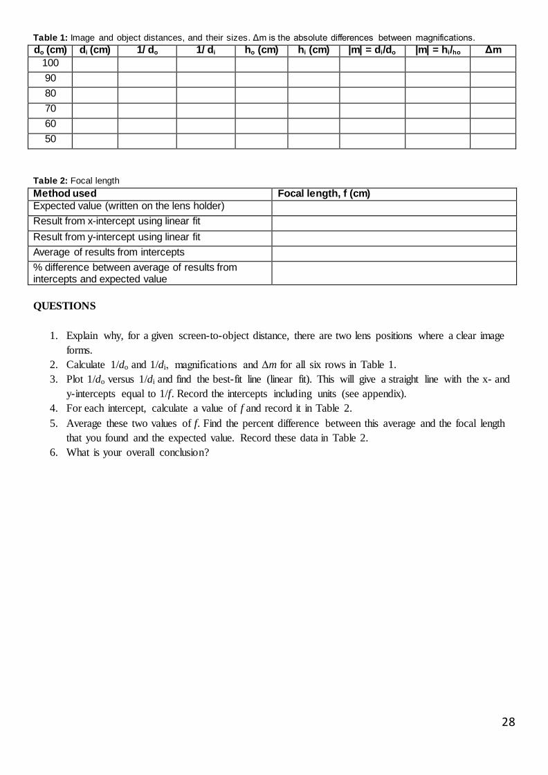
Table 1: Image and object distances, and their sizes. Δm is the absolute differences between magnifications.

do (cm) di (cm) 1/ do 1/ di ho (cm) hi (cm) |m| = di/do |m| = hi/ho Δm

100 90 80 70 60 50

Table 2: Focal length

Method used Focal length, f (cm)

Expected value (written on the lens holder) Result from x-intercept using linear fit Result from y-intercept using linear fit Average of results from intercepts % difference between average of results from intercepts and expected value

QUESTIONS

1. Explain why, for a given screen-to-object distance, there are two lens positions where a clear image

forms.

2. Calculate 1/do and 1/di, magnifications and Δm for all six rows in Table 1.

3. Plot 1/do versus 1/di and find the best-fit line (linear fit). This will give a straight line with the x- and

y-intercepts equal to 1/f. Record the intercepts including units (see appendix).

4. For each intercept, calculate a value of f and record it in Table 2.

5. Average these two values of f. Find the percent difference between this average and the focal length

that you found and the expected value. Record these data in Table 2.

6. What is your overall conclusion?

29

EXPERIMENT 10

LENS MAKER’s EQUATION

PURPOSE

In this experiment you will determine the focal length of the lens in two ways:

(a) by direct measurement using ray tracing and (b) by measuring the radius of curvature

and using the Lensmaker’s equation. The you will compare the results.

EQUIPMENT

Laser source

Milli-metric paper Positive and negative lenses Caliper

THEORY

Focal length, of a thick lens (f) in air can be calculated from the Lensmaker’s Equation:

(1)

where

n = index of refraction of the lens material (for acrylics n = 1.5 at λ = 650 nm)

R1 = radius of curvature of the first surface

R2 = radius of curvature of the second surface

t = center thickness of the lens

Figure 1 shows example converging lens with edge thickness w and lens diameter H.

Figure 1 A positive thick lens and its geometric parameters.H and w are the height (or diameter) and

the edge thickness of the lens, respectively where f is the back focal length.

30

PROCEDURE

1. Place a plastic bi-convex(positive) lens on the milli-metric paper as shown in Figure 2.

2. Turn on the laser source. Allow the parallel laser beam to fall on the lens. 3. Measure the focal length by using the lines on the paper. The focal point is where the rays cross.

4. Now, measure the height (H), the center thickness (t)and edge thickness (w) of the lens. 5. Compute the radii of curvatures as a function of H, t and w. And write down your observations. 6. Calculate the focal length of the lens using Eqn (1) for n = 1.5.

7. Calculate the percent difference between the two values of from step 3 and step 6. 8. Repeat your measurements for a plano-concave (negative lens). The focal point is where the

extension of outgoing rays cross.

Figure 2: Positive and negative lenses used in the experiment.

Table 1: The experimental data

Positive lens Negative lens

H (measured in mm) = H (measured in mm) = t (measured in mm) = t (measured in mm) =

w (measured in mm) = w (measured in mm) = R1 (measured in mm) = R1 (measured in mm) = R2 (measured in mm) = R2 (measured in mm) =

f (calculated in mm) = f (calculated in mm) = f (measured in mm) = f (measured in mm) =

Percentage difference = Percentage difference =

QUESTIONS

1. Derive an equation for the focal length of a lens as a function of measured geometric parameters (H,

t, w, R1, R2) given in Table 9.1.

2. Compute the percentage difference between measured and calculated values of the focal length for

both lenses and fill Table 1.

3. What is your conclusion?

31

EXPERIMENT 11

TELESCOPE AND MICROSCOPE

PURPOSE

In this experiment, you will construct a telescope/microscope and determine its magnification.

EQUIPMENT

Bench 2 Convex Lenses (+100 mm and +200 mm)

2 Convex Lenses (+250 mm and -150 mm [optional, for further study]) Screen Paper grid pattern (see Appendix), or a 14 × 16 grid of 1 cm squares

THEORY

Part I: The Astronomical Telescope

An astronomical telescope consists of two convex lenses. The astronomical telescope in this experiment will

form an image in the same place as the object (see Figure 1).

Figure 1: The simple astronomical (or Keplerian) telescope.

The magnification, m, of a two-thin-lens system is equal to the product of the magnifications of the

individual lenses:

(1)

Note that, if d01 goes to infinity and di1 + do2 = fo + fe then the magnification is given by:

(2)

fo = focal length of the objective lens

fe = focal length of the eyepiece lens

32

Figure 2:The setup

PROCEDURE for Telescope

1. Tape the paper grid pattern to the screen to serve as the object.

2. The +200 mm lens is the objective lens (the one closer to the object). The +100mm lens is the

eyepiece lens (the one closer to the eye). Place the lenses near one end of the optics bench and place

the screen on the other end (see Figure 2).Their exact positions do not matter yet.

3. Take a photograph of the grid pattern as shown in Figure 3. The grid lines are seen very small.

4. Without changing your horizontal position and distance to the screen, take another photograph as

indicated in Figure 4.

5. Now you have two digital images. Using a digital image processing tool (such as Microsoft Paint),

you can evaluate the magnification of the telescope as follows:

a) Measure the one side of the square in pixels in Figure 3 [for our case 10 px] b) Measure the one side of the square in pixels in Figure 4 [for our case 39 px]

c) The magnification is evaluated from

|m| = (one side of the big square) / (one side of the small square) = 39 px / 10px = 3.9.

33

Figure 3: Photo taken without telescope. Squares on the grid seem to be small. One side of the square is about 10

pixels. (You can obtain this data using MS paint program).

Figure 4: Photo taken with telescope. The squares on the grid are magnified compared to first figure. One side of the

big square is about 39 pixels. So, the magnification (m)can be calculated simply from

m = (one side of the big square) / (one side of the small square) = 39 px / 10 px = 3.9.

34

Part II: Galilean Telescope [optional]

Make a new telescope using -150 mm lens as the eyepiece and the +250 mm lens as the objective lens. Look

through it at a distant object. Adjust the distance between the lenses to focus the telescope with your eye

relaxed. How is the distance between the lenses related to their focal lengths? How does the image viewed

through this telescope differ from that of the previous telescope? Is the magnification positive or negative?

Part III: The Compound Microscope

A microscope magnifies an object that is close to the objective lens. The microscope in this experiment will

form an image in the same place as the object (see Figure 5).

Figure 5: The microscope

Magnification is computed as in Equation 1.

Figure 6: The setup for microscope

35

PROCEDURE for Microscope

1. Tape the paper grid pattern to the screen to serve as the object.

2. The +100 mm lens is the objective lens (the one closer to the object). The +200mm lens is the

eyepiece lens (the one closer to the eye). Place the lenses near the middle of the optics bench and

place the screen near the end of the bench (see Figure 6).

3. The rest of the procedure is same as in the Telescope.

4. Record your observation to Table 2.

QUESTIONS

1. Derive Equation 2.

2. Plot d01vs m graph of the telescope if di1 + do2 = fo + fe where fo = +200 mm and fe = +100 mm and

show that result asymptotically approaches to Equation 2.

3. Is the image in the telescope inverted or upright?

4. Is the image that you see through the telescope real or virtual?

5. Obtain the magnification of the telescope in your setup as described above and record you result in

Table 1.

6. Measure do1 and determine di1, do2, and di2 from thin lens equation.

7. Calculate the magnification using Equation 1 and record your results to the Table 1.

8. Repeat the calculations in s for microscope and record your results in Table 2.

9. What is your overall conclusion?

Table 1:Results for telescope

Position of objective lens = Position of eyepiece lens =

Position of the screen = Observed magnification (from digital image processing) =

do1 = di2 = di1 = do2 =

Calculated magnification = Percentage difference =

Table 2:Results for microscope

Position of objective lens = Position of eyepiece lens =

Position of the screen = Observed magnification (from digital image processing) =

do1 = di2 = di1 = do2 =

Calculated magnification =

36

A P P E N D I C E S

Appendix A: Experimental Errors

Appendix B: Basic Gnuplot Tutorial

Appendix C: Sample Written Report

37

Appendix A: Experimental Errors

A1. Introduction

In general, experiments are performed to test a theory and to compare with other independent experiments measuring the same quantity. When performing experiments, we should not consider that the job is over

once we obtain a numerical value for the quantity we are trying to measure. We should be concern not only with the measured value but also with its accuracy. The accuracy is derived from an experimental error for the measured quantity. For example, consider a measurement of the gravitational acceleration due to the

gravity is obtained as g = 9.77 ± 0.14 m/s2

We will mention about what we mean by the error (or accuracy) ± 0.14.

A2. Definitions

In this section, we will give some fundamental terms used in the measurement systems.

Error

The error is the difference between true value and measured value of a quantity.

Uncertainty

The uncertainty is the estimated error for a measurement. Since a true value for a physical quantity

may be unknown, it is sometimes not possible to determine the true error of the measurement. So, this term is more sensible for the error computations although the terms error and uncertainty are

used instead of each other in literature.

Percentage Error

Percentage error measures the accuracy of a measurement by the difference between a measured or experimental value E and a true or accepted value A. Percentage error is calculated by

(A.1)

Percentage Difference

Percentage difference measures precision of two measurements by the difference between the measured or experimental values E1 and E2 expressed as a fraction the average of the two values.

The equation to use to calculate the percent difference is:

(A.2)

Mean and Standard Deviation

For a set of n measurements {x1,x2,... ,xn}, the arithmetic mean, is defined by:

(A.3)

The Standard deviation is a measure that is used to quantify the amount of variation or dispersion of the measured values. It is defined as:

(A.4)

Note that the square of the standard deviation is known as variance.

38

The standard error of the mean is given by:

(A.5)

Final result obtained from this kind of repeated measurement should be reported in the form of

EXAMPLE A1: Consider the data of 10 different measurements for the mass density in g/cm3 of a liquid.

d = {1.10, 1.12, 1.09, 1.09, 1.07, 1.14, 1.11, 1.16, 1.07, 1.08}

The mean, standard deviation, variance and standard error of the measurement are as follows:

The result of the measurement is reported as d = 1.103 ± 0.009 g/cm3 or 1.103(9) g/cm

3.

A3. Measurement Errors for Some Devices (Instrumental Limitations)

The values of experimental measurements have uncertainties due to measurement limitations. Here we will show the uncertainty for two mostly used devices in the labs.

Ruler In Fig A1, the pointer indicates a value between 23 and 24 mm. With this millimeter scale one strategy is to take the center of the bin as the estimate of the value, the maximum error is then half the width of the bin. So in this case our measurement is 23.5 ± 0.5 mm. The value of 0.5 mm is the estimate of the random error.

Fig A1: Standard ruler has a maximum uncertainty of ± 0.5 mm. So, the value and its error is 23.5 ± 0.5 mm.

Digital Measuring Devices All digital measuring devices has a maximum uncertainty of the order of half its last digit. For example, in Fig 5, for the reading from a digital voltmeter, the uncertainty is ± 0.01/2 Volts. Thus, assuming the voltmeter is calibrated accurately, the value is 12.88 ± 0.005 V.

Fig A2: Digital voltmeter having a maximum uncertainty of ± 0.005 V for this reading. So the value and its error is 12.880 ± 0.005 V.

A4. Error Propagation In a typical experiment, one is seldom interested in taking data of a single quantity. More often, the data are processed through multiplication, addition or other functional manipulation to get final result. Experimental

39

measurements have uncertainties due to measurement limitations which propagate to the combination of variables in a function. In statistical data analysis, the propagation of error (or propagation of uncertainty) is the effect of measurement uncertainties (or errors) on the uncertainty of a function based on them. For a function of one variable, f(x), if x has a measurement error σx, then the associated error is computed from:

(A.6)

EXAMPLE A2: The radius of a circle is measured as r = 2.5 ± 0.3 cm. Calculate the area of the circle and its uncertainty.

The area of the circle is: Its derivative with respect to r is:

and the uncertainty in the area is:

Therefore , the area and its uncertainty is A = 19.6 ± 4.7 cm2.

In general, if x, y, z, … are independent variables having associated errors (standard deviations) σx, σy,σz, …

then the error for any quantity of the form f = f(x, y, z, …) derived from these errors can be calculated from:

(A.7)

Equation (A.7) is known as the error propagation formula used for uncorrelated (independent) measurements.

EXAMPLE A3: Suppose we wish to calculate the average speed (displacement/time) of an object. Assume the displacement is measured as x = 22.2 ± 0.5 cm during the time interval t = 9.0 ± 0.1 s. Then,

The derivatives are:

Finally the error in the speed is

Therefore, the reported result would be 2.47 ± 0.06 cm/s or 2.47(6) cm/s.

Exercise: Refractive index, n, of a glass is calculated by using Snell’s law: n = nair sin(θ1)/ sin(θ2) where

measured values and their estimated errors are given by nair = 1, θ1=61(1) degrees and θ2=36(1) degrees.

Calculate the refractive index of the glass and its uncertainty. [Answer: n = 1.488(24)].

r

40

Appendix B: Basic Gnuplot Tutorial

http://www.gnuplot.info

https://www.cs.hmc.edu/~vrable/gnuplot/using-gnuplot.html

http://people.duke.edu/~hpgavin/gnuplot.html

This is a basic tutorial for the Gnuplot program

which is a portable command-line driven graphing utility for

- Linux, - MS Windows - Mac

- Many other platforms.

Sep 2017

41

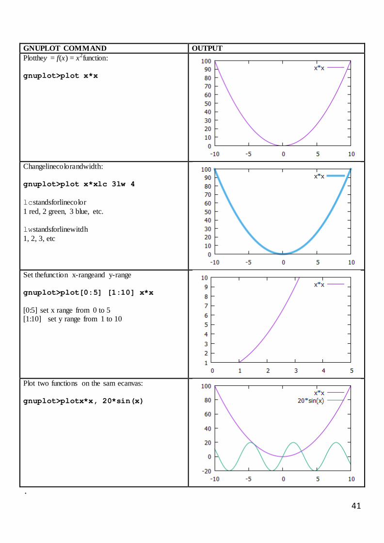
GNUPLOT COMMAND OUTPUT

Plotthey = f(x) = x2function:

gnuplot>plot x*x

Changelinecolorandwidth:

gnuplot>plot x*xlc 3lw 4

lcstandsforlinecolor

1 red, 2 green, 3 blue, etc.

lwstandsforlinewitdh

1, 2, 3, etc

Set thefunction x-rangeand y-range

gnuplot>plot[0:5] [1:10] x*x

[0:5] set x range from 0 to 5 [1:10] set y range from 1 to 10

Plot two functions on the sam ecanvas:

gnuplot>plotx*x, 20*sin(x)

.

42

GNUPLOT COMMAND OUTPUT

Remove key on the right-top of the figure:

gnuplot>unsetkey

gnuplot>plot x*x

set key : Shows the key on the figure

unsetkey : Removes the key on the figure

Set grid lines:

gnuplot> set grid

gnuplot> plot x*x

set grid : Shows the gridlines

unset grid : Removes the gridlines

Set titles:

gnuplot>reset

gnuplot> set grid

gnuplot>unset key

gnuplot>set title 'the title'

gnuplot>set xlabel 'time (s)'

gnuplot>set ylabel 'position (m)'

gnuplot>plot x*x

You can save all commands in a file called script. You

execute the script as follows. Assume that the script file name

is myfile.txt. Open myfile.txt on your Desktop folder and type

the following lines: reset

set grid

unset key

set title 'thetitle'

set xlabel 'time (s)'

set ylabel 'position (m)'

plot x*x

In gnuplot command window, change directory or useChDir

button on the tool bar.

gnuplot> cd 'C:\Users\Ahmet\Desktop'

gnuplot> load 'myfile.txt'

43

.

GNUPLOT COMMAND OUTPUT

Plot the function y = f(x, y) = x2+ y2 :

gnuplot>splot x*x+y*y

Plot the function y = f(x, y) = sin(x)*cos(y)

for the given range

gnuplot>unset key

gnuplot>splot [x=-3:3] [y=-3:3] sin(x)*cos(y)

Plot the function y = f(x, y) = xy with points

gnuplot>splot x*y with points

Plot a toroid

gnuplot>set nokey

gnuplot>set parametric

gnuplot>set hidden3d

gnuplot>set view 30

gnuplot>set isosamples 30,20

gnuplot>splot [-pi:pi][-pi:pi]

cos(u)*(cos(v)+3),

sin(u)*(cos(v)+3),sin(v)

.

44

GNUPLOT COMMAND OUTPUT

Consider you have the following data file saved in

your Desktop as “data.txt”. # X Y

1 25

2 30

3 32

4 35

5 28

6 25

7 22

8 21

gnuplot>plot 'data.txt'

gnuplot> plot 'data.txt' pt 7 ps 1.5

pt :point type (1,2,3, etc)

ps :point size

Consider you have the following data file saved in

your Desktop as “data3d.txt”.

# X Y Z

1 25 2.5

2 30 3.1

3 32 5.0

4 35 5.1

5 28 3.0

6 25 2.7

7 22 1.8

8 21 1.5

gnuplot>splot 'data3d.txt' matrix

withlines

Plotc olumn1 vs colum3 and connect data points with lines gnuplot>plot 'data3d.txt' using 1:3

withlines

45

Linear fit using Gnuplot

Example 1: The distance required to stop an automobile is a function of its speed. The following data is collected to get this relationship:

First column is the speed of the car in km/h and second column is measured stopping distance in meter.

The following script is useful for linear fitting:

In gnuplot command line type: gnuplot> load 'fitter.txt'

Final set of parameters Asymptotic Standard Error

======================= ==========================

a = 0.394853 +/- 0.028 (7.09%)

b = -5.95294 +/- 1.446 (24.29%)

24 4.8

32 6.0

40 10.2

48 12.0

64 18.0

80 27.0

# fitter.txt

reset

set grid

unset key

set title 'linear fit example'

set xlabel 'velocity (km/h)'

set ylabel 'stoping distance (m)'

f(x) = a*x + b

fit f(x) 'data.txt' via a,b

plot 'data.txt' pt 5 ps 1, f(x) lc 1

46

Non linear fit using Gnuplot

Example 2: The same data in Example 1 can be fit to a non-linear function (say) y = ax2 + bx.

The script is

In gnuplot command line type: gnuplot> load 'fitter.txt'

Final set of parameters Asymptotic Standard Error

======================= ==========================

a = 0.00257446 +/- 0.0003253 (12.64%)

b = 0.127548 +/- 0.02105 (16.5%)

24 4.8

32 6.0

40 10.2

48 12.0

64 18.0

80 27.0

# fitter.txt

reset

set grid

unset key

set title 'linear fit example'

set xlabel 'velocity (km/h)'

set ylabel 'stoping distance (m)'

f(x) = a*x**2 + b*x

fit f(x) 'data.txt' via a,b

plot 'data.txt' pt 5 ps 1, f(x) lc 1

47

Example 3: Consider the content of a file named data.txt:

First column is the angle in radian and second column is measured value of offset distance d in mm in the Optical Slab experiment. In gnuplot program, the fitting of Equation to find n to this data is as follows:

gnuplot> h = 60 # thickness of the slab in mm

gnuplot> f(x) = h*sin(x)*(1-cos(x)/sqrt(n**2-sin(x)**2))

gnuplot> fit f(x) 'data.txt' via n

Final set of parameters Asymptotic Standard Error

======================= ==========================

n = 1.50842 +/- 0.003713 (0.2462%)

gnuplot> set xlabel('Angle (rad)')

gnuplot> set ylabel('Distance, d (mm)')

gnuplot> plot 'data.txt', f(x) lc 3

Therefore the index of refraction is found as:

n = 1.50842 +- 0.003713

0.17453 3

0.34907 7

0.52360 12

0.69813 17

0.87266 23

1.04720 31

1.22173 40

48

Appendix C: Sample Written Report

In this section, we will present you a sample report (starting from the next page), obtained in the Snell’s Law

Refraction (Experiment 4).

Try to obey the rules as in this sample.

Bring your reports to lab research assistant on time (weekly).

Include to your report the data sheet(s) signed by the lab assistant in the lab.

49

Gaziantep University

Department of Optical and Acoustical Engineering

OPAC 103 Geometric Optics Laboratory

LAB REPORT FOR EXPERIMENT 4

SNELL’S LAW OF REFRACTION

Group 2 Members

Ahmet BİNGÜL

Mustafa KILIN

Şirin UZUN

06 Oct 2017

50

The data we have obtained in the experiment is as follows:

Angle of incidence

θ1 (in degrees) Angle of

refraction

θ2 (in degrees) sin(θ1) sin(θ2)

index of

refraction n

5 3 0.087156 0.052336 1.6653

10 7 0.173648 0.121869 1.4249

15 10 0.258819 0.173648 1.4905

20 13 0.342020 0.224951 1.5204

25 16 0.422618 0.275637 1.5332

30 19 0.500000 0.325568 1.5358

35 22 0.573576 0.374607 1.5311

40 25 0.642788 0.422618 1.5210

45 28 0.707107 0.469472 1.5062

50 31 0.766044 0.515038 1.4874

55 33 0.819152 0.544639 1.5040

60 35 0.866025 0.573576 1.5099

65 37 0.906308 0.601815 1.5060

70 39 0.939693 0.629320 1.4932

Average, <n> = 1.5163

Standard Deviation, σ = 0.0511

Standard Error, σE = 0.0137

Answers of Questions:

1.The D-shaped material has an advantage in this experiment. First, the light enters from its flat surface and

refracts according to Snell’s law, Equation 1 in the lab sheet. Then the light travels inside the material and

leaves it from the circular side. If the light enters nearly the center of the D-shape as in Figure 1, then it hits

the circular face at right angle (perpendicular). As a result, the light leaves the material without refracting.

Therefore, we can only apply Snell’s law on the first surface.

Figure 1: Light follows the path AOB. At point O it refracts. At point B, it will leave the D-Shape without

refracting since Snell’s law does not work for the light rays normally entering or leaving the surface.

2. From the table, the mean value of the data and its standard error is:

n = 1.5163 +/- 0.0137

Or the interval that encloses the true index of refraction (with 68% confidence level) is:

n = [1.5026, 1.5300].

51

3. Alternatively, we can extract the index of refraction using linear fitting. Figure 2 shows the result of

fitting procedure applied for our data where sin(θ2) values are plotted in x-axis and sin(θ1) values are plotted

in y-axis. According to Snell’s law sin(θ2) = n sin(θ1), that is, sin(θ2) is linearly proportional to sin(θ1) and

the proportionality constant (or the slope) is n, the index of refraction. Therefore, the slope of the line

obtained from fitting procedure gives the index of refraction. The extracted value using gnuplot program is:

n = 1.50665 +/- 0.004418.

Figure 2: Linear fitting result using gnuplot. The slope of the best fit line gives the index of refraction

The gnuplot script (called fitter.txt) used to extract n is given below. The file data.txt contains the

values of sin(θ2) vs sin(θ1) values in the form of two columns, respectively. The fitting result is also given.

# fitter.txt

reset

set grid

unset key

set title 'Verification of Snell

Law'

set xlabel 'sin(theta2)'

set ylabel 'sin(theta1)'

f(x) = n*x

fit f(x) 'data.txt' via n

plot 'data.txt' pt 5 ps 1, f(x) lc 1

Final set of parameters Asymptotic Standard Error

======================= ==========================

n = 1.50665 +/- 0.004418 (0.2932%)

4. Conclusion

In this experiment, Snell’s law of refraction is validated by using two different methods, the arithmetic mean

and linear fitting method. The aim of the experiment is to measure the index of refraction of a material by

collecting several pairs of the angle of incidence and angle of refraction data. The results of the method are

n = 1.5163 +/- 0.0137 and n = 1.50665 +/- 0.004418, respectively. The actual value of the index of

refraction is n = 1.5. Hence, the percentage errors are as follows:

P.E.(mean) = 100% x (1.51630-1.5000)/1.5000 = 1.1 %

P.E.(fit) = 100% x (1.50665-1.5000)/1.5000 = 0.4 %

The results of both methods are quite consistent with the expected value. However, the fitting method

exhibits a better performance since its associated error and its percentage error is much smaller.