CONFRONTING MODEL MISSPECIFICATION INMACROECONOMICSDANIEL F. WAGGONER AND TAO ZHAAbstra t. We onfront model misspe i� ation in ma roe onomi s by proposing ananalyti framework for merging multiple models. This framework allows us to 1)address un ertainty about models and parameters simultaneously and 2) tra e outthe histori al periods in whi h one model dominates other models. We apply theframework to a ri hly parameterized DSGE model and a orresponding BVAR model.The merged model, �tting the data better than both individual models, substantiallyalters e onomi inferen es about the DSGE parameters and about the implied impulseresponses. I. Introdu tionA sto hasti dynami equilibrium, indexed by a parameterized model, is a likelihoodfun tion. Given the likelihood and the prior density of model parameters, one ansimulate the posterior distribution and ompute the marginal data density (MDD).The MDD is then used to measure how well the model is �t to the data.Consider the situation in whi h there are multiple models on the table. The onven-tional pro edure for model sele tion is to ompare MDDs amongst individual models.1Sin e it is not un ommon that the MDD implied by one of the models is overwhelm-ingly higher than the MDDs implied by others, this pro edure often ends up withthe sele tion of one model at the ex lusion of others. One primary example is that alinearized dynami sto hasti general equilibrium (DSGE) model su h as Smets andWouters (2007) an easily trump a standard Bayesian ve tor autoregression (BVAR)Date: November 29, 2010.Key words and phrases. Merged model, misspe i� ation, state-dependent weights, model un er-tainty, parameter un ertainty, impulse responses, poli y analysis.JEL lassi� ation: C52, E2, E4.We thank Frank Diebold, John Geweke, Frank S horfheide, and Chris Sims for helpful dis ussions.The views expressed herein are those of the authors and do not ne essarily re�e t the views of theFederal Reserve Bank of Atlanta or the Federal Reserve System.1We impli itly assume that the prior weight is the same for all models. If the prior weight variesa ross models, we simply adjust the Bayes fa tors and al ulate the posterior odds ratios.1

CONFRONTING MODEL MISSPECIFICATION 2model.2 The impli ation is that the BVAR an be simply repla ed by the DSGE modelfor poli y analysis.Despite su h overwhelming eviden e presented by the posterior odds ratios in favor ofone model, e onomists nonetheless ontinue to use both the DSGE and BVAR modelsin ma roe onomi analysis. The tension between what the onventional pro edure on ludes and what a tually transpires is a mere manifestation of in reasing on ernsabout model misspe i� ation by hoosing a parti ular model (a parti ular likelihood)and ategori ally reje ting other models. Poli ymakers, as well as a ademi resear hers,re ognize that models are only approximations (Hansen and Sargent, 2001; Bro k,Durlauf, and West, 2003; Sims, 2003). Indeed, they seldom rely on one single modeleven though this model �ts better than other models a ording to the posterior odds riterion, be ause they know thatWe onfront model misspe i� ation by proposing a Bayesian approa h to mergingmultiple models. The merged model assigns state-dependent weights to predi tivedensities ( onditional likelihoods) implied by di�erent models so that the relative im-portan e of ea h model hanges a ross time. This new methodology, built on Gewekeand Amisano (forth oming), is motived by pra ti al poli y analysis dealing with situ-ations where there are multiple ompeting models and ea h model explains (predi ts)an observed out ome better than other models but only for ertain episodes. An infor-mal way for poli y analysis is to employ a di�erent model at a di�erent time. Unlikethe onventional model-averaging method, our Markov-swit hing approa h not onlyassigns a weight of relative importan e to ea h model but, more importantly, allows re-sear hers to tra e out the periods in whi h the data give the most weight to a parti ularmodel.We apply our analyti framework to two widely used models: a ri hly parameter-ized DSGE model and a orresponding BVAR model. The MDD for the DSGE modelis mu h higher than the BVAR model. The onventional Bayesian model-averagingmethod would imply that the BVAR model should re eive nearly zero weight, a pathol-ogy dis ussed in Sims (2003). Our Bayesian approa h over omes this pathology. Themerged model does not degenerate into the DSGE model or the BVAR model. To the ontrary, our estimation indi ates that the BVAR model dominates the DSGE model2For sensitivity analysis, we also onsider a ase in Se tion VI.4, where the BVAR model trumpsthe DSGE model.

CONFRONTING MODEL MISSPECIFICATION 3throughout two thirds of the history. The merged model, assigning nontrivial state-dependent weights to both models, �ts the data onsiderably better than either theDSGE model or the BVAR model.The rest of the literature has often treated the BVAR model as a ben hmark to gaugehow misspe i�ed the DSGE model is. Our estimated results hallenge this thinkingbe ause both the BVAR model and the DSGE model may be potentially misspe i�ed.Rather than divor ing the data analysis from a parti ular model whose �t may not beas good, the estimation of our merged model indi ates that both DSGE and BVARmodels are operative but at di�erent times.Our methodology makes it e onometri ally implementable to establish the two-way ommuni ation between the theoreti al DSGE model and the atheoreti al BVARmodel. We �nd that the posterior distributions of a number of key DSGE parameters hange substantially when we in orporate the BVAR model in the merged model spa e.The error bands around impulse responses are predominately wider as the data implymore un ertainty about the DSGE model when the merged model is estimated. Therelative importan e of a stru tural sho k in the DSGE model in explaining ma roe o-nomi �u tuations is in�uen ed heavily by the presen e of the BVAR model. Thus,our approa h integrates the two types of un ertainty, model un ertainty and parameterun ertainty, in one oherent framework.II. Literature reviewOur key assumption in this paper is that the true data generating pro ess may notbe among the models whose fore asts are ombined. This insight appears in Diebold(1991), who argues that the standard Bayesian posterior-odds fore ast averaging shouldbe re-thought. Geweke and Amisano (forth oming) propose a method of pooling themodels by ombining the predi tive densities, whi h are onsistent with out-of-samplefore asts. Although Geweke and Amisano (forth oming) do not take a stand on the truedata generating pro ess, the log predi tive s ore of pooled models tends to dominatethe s ore of ea h individual model in the pool as the sample be omes large. Thisresult is onsistent with the extension of Geweke and Amisano (forth oming)'s idea byFisher and Waggoner (2010), who assume expli itly that the data generating pro essis a mixture of multiple models.Our e onometri methodology builds on these previous works. We show that state-dependent weights not only in lude Fisher and Waggoner (2010) as a spe ial asebut also gives a di�erent interpretation about the relative importan e of ea h model by

CONFRONTING MODEL MISSPECIFICATION 4estimating the probability that ea h model is hosen at time t.3 Using the log predi tives ore, Geweke and Amisano (forth oming) estimate the weights of models while takingthe parameters in ea h model as given. Unlike Geweke and Amisano (forth oming),we estimate the weights and the parameters of all the models jointly. One of our key�ndings is that the estimated parameters for the merged model are di�erent from thosewhen the models are estimated separately.Del Negro and S horfheide (2004) address potential BVAR misspe i� ation by in-trodu ing the prior implied by a DSGE model into a BVAR model. We extend theiridea by allowing for the two-way ommuni ation between the two models. Both theDSGE prior and the BVAR prior play an integral part of model estimation. Moreover,the two likelihoods intera t with ea h other in forming the merged likelihood.Cogley and Sargent (2005) study an e onomy in whi h agents, fa ing model un er-tainty, ompute the posterior odds ratios over three models and make de isions byBayesian model averaging. As pointed out by Sims (2003) and Geweke and Amisano(forth oming), one an en ounter the pathology that the odds ratios lead to sele t-ing only one model and reje ting all other models. By estimating the state-dependentweights and the parameters of the models jointly, we provide an empiri ally operationalway to implement Sims (2003)'s idea of ��lling in the gap� between DSGE and BVARmodels by over oming the di� ulties inherent in Bayesian model averaging.4III. Markov-swit hing frameworkTo integrate model un ertainty and parameter un ertainty in one merged framework,we propose a Bayesian approa h to modeling state-dependent weights for a linear om-bination of predi tive densities produ ed by di�erent models. Our key assumption isthat the observed data at time t, yot , is generated from the following predi tive densityp(

yt | Yot−1,Θ, Q, w

)

=

n∑

i=1

w∗

i,tp(

yt | Yot−1,Θi,Mi

)

,wherew∗

i,t =

h∑

st=1

wi,stp(

st | Yot−1,Θ, Q, w

)

,3West and Harrison (1997) present a similar idea of allowing the weights of ea h model time-varyingin dynami fore asting exer ises.4Hansen and Sargent (2001) and Sims (2003) advo ate a large model spa e. In our framework, thisadvi e orresponds to in reasing the number of individual models in the merged model spa e.

CONFRONTING MODEL MISSPECIFICATION 5p(

yt | Yot−1,Θi,Mi

) is the predi tive density of yt onditional on the parameters ofmodel i and the observed data up to time t − 1, Y ot−1 =

{

yo1, · · · , yot−1

}, Θi is a set ofparameters for model i, and wi,st is the probability weight given to model i when thestate, st, o urs at time t with wi,st ≥ 0 and ∑ni=1wi,st = 1. The state variable, st,follows a Markov pro ess with the transition matrix Q, where Prob [st = k | st−1 = j] =

qk,j for k, j = 1, . . . , h.5 Note thatΘ = {Θ1, · · · ,Θn}, w = {wi,k} for k = 1, . . . , h, i = 1, . . . , n.We use the notation �Mi� in p

(

yt | Yot−1,Θi,Mi

) be ause we will ompare the marginaldata density of model i, denoted by p (Y oT | Mi), with the marginal data density of the omplete model, denoted by p (Y o

T | M).The log likelihood fun tion is thus given bylog p (Y o

T |Θ, Q, w) =T∑

t=1

log p(

yt | Yot−1,Θ, Q, w

)

=

T∑

t=1

log

[

n∑

i=1

(

h∑

st=1

wi,stp(

st | Yot−1,Θ, Q, w

)

)

p(

yot | Yot−1,Θi,Mi

)

]

,where the parameters Θ, Q, and w are to be estimated jointly.Whether model i will be preferred by the data depends on the state st. We use therandom variable ξt ∈ {1, . . . , n} to index the model hosen at time t. This randomvariable obeys the onditional probability:p (ξt | st) = wst,ξt ,where ∑n

ξt=1 p (ξt | st) = 1 be ause ∑nξt=1wst,ξt = 1. Although ξt is not a Markov-pro ess itself, the joint pro ess (st, ξt) is.Proposition 1. The joint pro ess (st, ξt) is a Markov pro ess with the expanded transi-tion matrix Prob [(st, ξt) = (k, i) | (st−1, ξt−1) = (j, g)] = qk,jwi,k,for j, k = 1, . . . , h and g, i = 1, . . . , n.Proof. The proof follows from the basi onditional probability theory by noting that

p (st, ξt | st−1, ξt−1) = p (st | st−1, ξt−1) p (ξt | st, st−1, ξt−1) = p (st | st−1) p (ξt | st) .

�5As shown in Sims, Waggoner, and Zha (2008), qkj an also depend on the observed data Y ot−1.

CONFRONTING MODEL MISSPECIFICATION 6Proposition 1 formulates the way we implement our estimation strategy. Sin e therestri tions imposed on the expanded transition matrix in Proposition 1 satisfy the onditions spe i�ed in Sims, Waggoner, and Zha (2008), one an apply their estimationmethod dire tly to our framework of merging individual models.IV. Identifi ation and reinterpretationIn this se tion we dis uss the identi� ation of state-dependent weights and reinterpretwhat onstant weights used in the literature mean from the ex ante point of view.IV.1. General identi� ation issue. In general, wi,k and p(

st | Yot−1,Θ, Q, w

) an beidenti�ed separately. To see this point, onsider the following ase with h = 2 andn = 2:

w1,1 w1,2

w2,1 w2,2

w3,1 w3,2

[

p(

st = 1 | Y ot−1,Θ, Q, w

)

p(

st = 2 | Y ot−1,Θ, Q, w

)

]

=

w∗

1,t

w∗

2,t

w∗

3,t

.For any given w∗

i,t and p(

st | Yot−1,Θ, Q, w

), there are three equations but four unre-stri ted weights wi,k and it appears that we always have more than one solution. This on lusion is not true, however. Sin e both w∗

i,t and p(

st | Yot−1,Θ, Q, w

) hange overtime but wi,k are onstant, we do not have more than one solution and may indeedhave no solution at all for some t or st. This results means that we annot arbitrarily hange w∗

i,t and p(

st | Yot−1,Θ, Q, w

) while keeping wi,k the same a ross time. Thus, we an in general identify wi,st.IV.2. Strengthening identi� ation. As the number of models or the number ofstates in reases, the number of free parameters in the expanded transition matrixin reases at an even faster speed, making it ne essary to impose further restri tions toavoid over�tting and at the same time strengthen the identi� ation of wi,st. To a hievethis goal, we let h = n, wi,st = 1 when st = i, and wj,st = 0 when st 6= j . Thus, whenthe state st is realized, only one of the models is operative. Sin e one an never besure of whi h state is realized, one an never be sure of whi h model is operative, evenafter observing all the data. One an, however, ompute the smoothed probability ofthe state, p(st | Y oT , Θ, Q, w

), where the supers riptˆdenotes the posterior estimate.The probability enables one to gauge how likely a parti ular model is sele ted. In ourappli ation, we will report this posterior probability throughout the history.

CONFRONTING MODEL MISSPECIFICATION 7IV.3. Reinterpretation. Although we know whi h model is operative given the ur-rent state st, there is un ertainty about models ex ante (i.e., at time t−1) and fore astsof e onomi variables will in general depend on multiple models through the transitionmatrix. Thus, for the purpose of poli y fore asts, it is ex ante un ertainty that matters.Moreover, this un ertainty presents a di�erent interpretation of onstant weights usedin the literature, as shown in the following proposition.Proposition 2. If qi,j = qi,k = qi for i, j, k = 1, . . . , n, it must be true that w∗

i,t = qi.Proof. Be ause qi,j = qi,k, the probability of swit hing to the urrent state st is thesame no matter what the state at time t − 1 is. This result means that all the pastdata are irrelevant in inferring about the probability of the urrent state. It followsthatp(

st = i | Y ot−1,Θ, Q, w

)

= qi.From the de�nition of w∗

i,t, we havew∗

i,t =h∑

st=1

wi,stp(

st | Yot−1,Θ, Q, w

)

= wi,ip(

st = i | Y ot−1,Θ, Q, w

)

= qi.

�It is, perhaps, not surprising that onstant weights are a spe ial ase of our Markov-swit hing framework. What is new from Proposition 2 is that a onstant weight isabout the relative importan e of the model only at time t− 1 and the model's weightwill hange on e we have the data beyond time t − 1. Given all the data, moreover,our Markov-swit hing framework enables us to reinterpret this history by tra ing outthe periods in whi h a parti ular model is more relevant than others, even when all theweights are onstant. V. Appli ationWe apply the framework presented in Se tion III to two widely used models: amedium-s ale DSGE model and a BVAR model. The DSGE model is based on Liu,Waggoner, and Zha (2010). The large part of the model is the same as Altig, Chris-tiano, Ei henbaum, and Linde (2004) and Smets and Wouters (2007) with the notableex eptions that (1) some real rigidity is introdu ed, as in Chari, Kehoe, and M Grat-tan (2000), by assuming the existen e of �rm-spe i� fa tors (su h as land) su h thatthe sum of ost shares of apital and labor inputs is less or equal to one and (2) a

CONFRONTING MODEL MISSPECIFICATION 8sho k to the depre iation in physi al apital is introdu ed as a stand-in for e onomi obsoles en e of apital (see Appendix B for some details of the model).The DSGE model is �t to eight quarterly variables: quarterly growth of real per apita GDP (∆ log Y Datat ), quarterly growth of real per apita onsumption (∆ logCData

t ),quarterly growth of real per apita investment in apital goods unit (∆ log IDatat ), quar-terly growth of the real wage (∆ logwDatat ), the quarterly GDP-de�ator in�ation rate(πDatat ), quarterly growth of per apita hours (∆ logLData

t ), the federal funds rate(FFRDatat ), and quarterly growth of investment-spe i� te hnology (∆ logQData

t ) asmeasured by the inverse of the relative pri e of investment. A detailed des ription ofthe data is given in Appendix A. The data in the initial four quarters from 1960:I to1960:IV are used to obtain the initial ondition at 1961:I for the Kalman �lter. Thus,the e�e tive sample used for model evaluation is from 1961:I to 2010:II.The BVAR model has the same eight variables as the DSGE model; and it has fourlags from 1960:I to 1960:IV so that the e�e tive sample is also from 1961:I to 2010:II.To make our BVAR model omparable with the DSGE literature, we follow Smets andWouters (2007) and use the standard �Minnesota-like� prior with the hyperparametervalues µ1 = µ2 = µ3 = 1.5, and µ4 = 1.3 where µ1 ontrols overall tightness ofthe random walk prior, µ2 ontrols relative tightness of the random walk prior onthe lagged oe� ients, µ3 ontrols relative tightness of the random walk prior on the onstant term, and µ4 ontrols tightness of the prior that dampens the errati samplinge�e ts on lag oe� ients (lag de ay).6The prior for the DSGE model is reported in Tables 1 and 2. Instead of spe ifyingthe mean and the standard deviation, we use the 90% probability interval to ba kout the hyperparameter values of the prior distribution. The intervals are generallyset wide enough to allow for the possibility that the posterior mode is lose to or onthe boundary of the parameter spa e. It also allows for multiple lo al posterior peaks(Del Negro and S horfheide, 2008). Our approa h is ne essary to deal with skeweddistributions and allows for reasonable hyperparameter values in ertain distributions,su h as the Inverse-Gamma, where the �rst two moments may not exist.For many parameters with the Beta prior distribution, su h as the habit parameterand the persisten e parameters in sho k pro esses, we insist on a positive probabilitydensity at the value 0 to allow for the possibility of no habit and no persisten e at all;we also insist on zero probability density at the value 1 to maintain the assumption that6In Se tion VI.4, we study another standard prior proposed by Sims and Zha (1998).

CONFRONTING MODEL MISSPECIFICATION 9the e onomy is on the balan ed growth path. Consequently, the two hyperparametervalues for the Beta prior are set at 1.0 and 2.0.The prior for the labor share and apital share is the Beta distribution with therestri tion α1 + α2 ≤ 1 su h that the produ tion te hnology requires �rm-spe i� fa tors (Chari, Kehoe, and M Grattan, 2000). The bounds for the α1 values in the90% probability interval are 0.3 and 0.4 and those for α2 are 0.5 and 0.7. With therestri tion α1 + α2 ≤ 1, however, the joint 90% probability region would be somewhatdi�erent.The prior for the inverse Fris h elasti ity η follows the Gamma distribution. We hoose the 2 hyper-parameters of the Gamma distribution su h that the lower bound(0.2) and the upper bound (10.0) of η orrespond to the 90% probability interval. Thisprior range for η implies that the Fris h elasti ity lies between 0.1 and 5.The lower and upper bounds of prior distributions are spe i�ed in Table 1 for theparameters λq, λ∗, β, σu, S ′′, δ, ξp, γp, ξw, γw, φπ, φy, and π∗. Using these wide bounds,we ba k out the two hyperparameter values for the orresponding prior distributions.The Gamma prior for the average net pri e markup µp−1 is the same as the Gammaprior for the average net wage markup µw − 1. By setting the �rst hyperparameter ofthis prior to be 1.0, we allow for a positive probability that the net markups may bezero. This generality (a less stringent prior) turns out to be riti al as our posteriorestimates of µp − 1 and µw − 1 are nearly zero. We set the se ond hyperparameter ofthe Gamma prior at 5.5 su h that the implied 90% probability bounds are wide enough(from 0.0094 to 0.5446).The prior for the parameter ρgz, apturing the impa t of te hnologi al improvementon government spending, is the Gamma distribution with the 90% probability boundsgiven by [0.2, 3.0].The standard deviation of ea h of the 8 sho ks has the Inverse Gamma prior dis-tribution with the 90% probability bounds given by [0.0005, 1.0]. These wide boundsare ne essary to take a ount of the possibility that some sho ks may have very smallvarian es while others may have very large varian es. With these bounds, there existno moments for the Inverse Gamma prior. One an still, however, ba k out the twohyperparameter values as reported in Table 2.The transition from one model to the other has the following matrix form:

Q =

[

q11 q12

q21 q22

]

,

CONFRONTING MODEL MISSPECIFICATION 10where∑2i=1 qij = 1 for j = 1, 2. Following Sims, Waggoner, and Zha (2008), we expressa prior belief that the average duration for a model to remain dominant is between sixand seven quarters. The belief implies that the hyperparameter in the exponent of qiiin the Diri hlet prior density is 5.6667 and the other hyperparameter is 1.0. This priorsetting allows for the possibility that model i dominates other models all the time (i.e.,

qii = 1). Table 2 reports the orresponding 90% probability interval.VI. Measuring misspe ifi ationIn this se tion we quantify the degree of DSGE model misspe i� ation by 1) om-puting the MDDs for the DSGE and BVAR models against the MDD for the mergedmodel and 2) tra ing out the posterior probabilities of ea h model a ross time. Wethen dis uss a variety of e onomi impli ations of this misspe i� ation. Although bothBVAR and DSGE models are misspe i�ed, we fo us on the DSGE model by omparingthe estimated results of the merged model to those of the DSGE model alone.VI.1. Model �t. We ompute the MDDs for the merged model, the DSGE modelalone, and the BVAR model alone. Table 5 reports log values of these MDDs. Forthe BVAR model, there is an analyti al solution for al ulating the MDD so that thereported log value of MDD has negligible numeri al errors. For the DSGE model andthe merged model, however, numeri al errors are nontrivial. We use two di�erent MonteCarlo methods to ompute MDDs. One method is the trun ated modi�ed harmoni mean (MHM) method proposed by Sims, Waggoner, and Zha (2008); the other method, alled the �Müeller method,� is developed by Ulri h Müeller at Prin eton University.7The two methods an give di�erent results due to numeri al errors and we report therange of estimates of the MDDs in Table 5.8The log value of the MDD for the DSGE model is about 50 above log MDD forthe BVAR. The onventional Bayesian averaging pro edure would give the BVAR es-sentially zero weight. The merged model, unlike the onventional Bayesian averagingpro edure, not just ombines the two distin t models but also expands the parameterspa e by estimating the parameters of both models and the weights jointly. Conse-quently, both models are operative as dis ussed in Se tion VI.2. The resulting MDD7See Liu, Waggoner, and Zha (2010) for a detailed des ription of the Müeller method.8To ensure the a ura y, 20 million posterior draws and 2 million proposal draws are simulated.For the merged model, the simulation takes about 30 days or two full days by availing itself to omputational parallelism on a luster of 15 modern omputers.

CONFRONTING MODEL MISSPECIFICATION 11for the merged model is about 100 in log value above the MDD for the DSGE model.This magnitude gives a sense of how misspe i�ed both models are.VI.2. Posterior estimates. The prior spe i�ed for the DSGE model is looser andmore agnosti than most priors in the DSGE literature. The agnosti prior omesalso with the pri e: sin e the likelihood fun tion for the merged model is ompli atedand full of multiple lo al peaks, the resulting posterior density fun tion is ompli atedas well. The non-Gaussian nature of the posterior density implies that the posteriormean may have a very low (joint) probability and thus annot represent the most likelyout ome for the model. The posterior mode is, by de�nition, the most probable pointin the parameter spa e, regardless of how non-Gaussian and ompli ated the shape ofthe posterior probability density is. Moreover, using a point in the neighborhood ofthe posterior mode as a starting point for the MCMC algorithm avoids the situationwhere a long sequen e of posterior draws gets stu k in the low probability region dueto a poor starting point.To �nd the posterior mode, we ombine the hill- limbing quasi-Newton (Broyden-Flet her-Goldfarb-Shanno � BFGS) algorithm with o asional downhill movementsgenerated by MCMC draws. Tables 3 and 4 report the posterior-mode estimates ofthe DSGE model parameters along with the 90% marginal probability intervals. Inthese tables we ontrast the estimated results for the merged model to those for theDSGE model alone. There are a few instan es in whi h the estimated results from themerged model are similar to those from the DSGE model when estimated alone. Theprobability interval of β is a tually smaller in the merged model than in the DSGEmodel alone. The estimate of the average pri e markup is lose to zero, similar to theestimate in the DSGE model when treated alone. This result implies that the demand urve for di�erentiated goods is very �at. Thus, a small in rease in the relative pri e an lead to large de lines in relative output demand. Even if �rms an re-optimizetheir pri ing de isions frequently, they hoose not to adjust their relative pri es toomu h. In other words, the small average markup and thus the large demand elasti itybe ome a sour e of strategi omplementarity in �rms' pri ing de isions.The general pattern, as indi ated by the 90% probability intervals, is that the mergedmodel exposes more un ertainty about the estimated DSGE parameters than what isimplied when the DSGE model is treated as the truth and estimated alone. In many ases, su h as the inverse Fris h elasti ity of labor supply (η) and the urvature ofthe apital utilization ost fun tion evaluated at the steady state (σu), the probabilitydistributions have hanged so mu h that the posterior estimates are very di�erent.

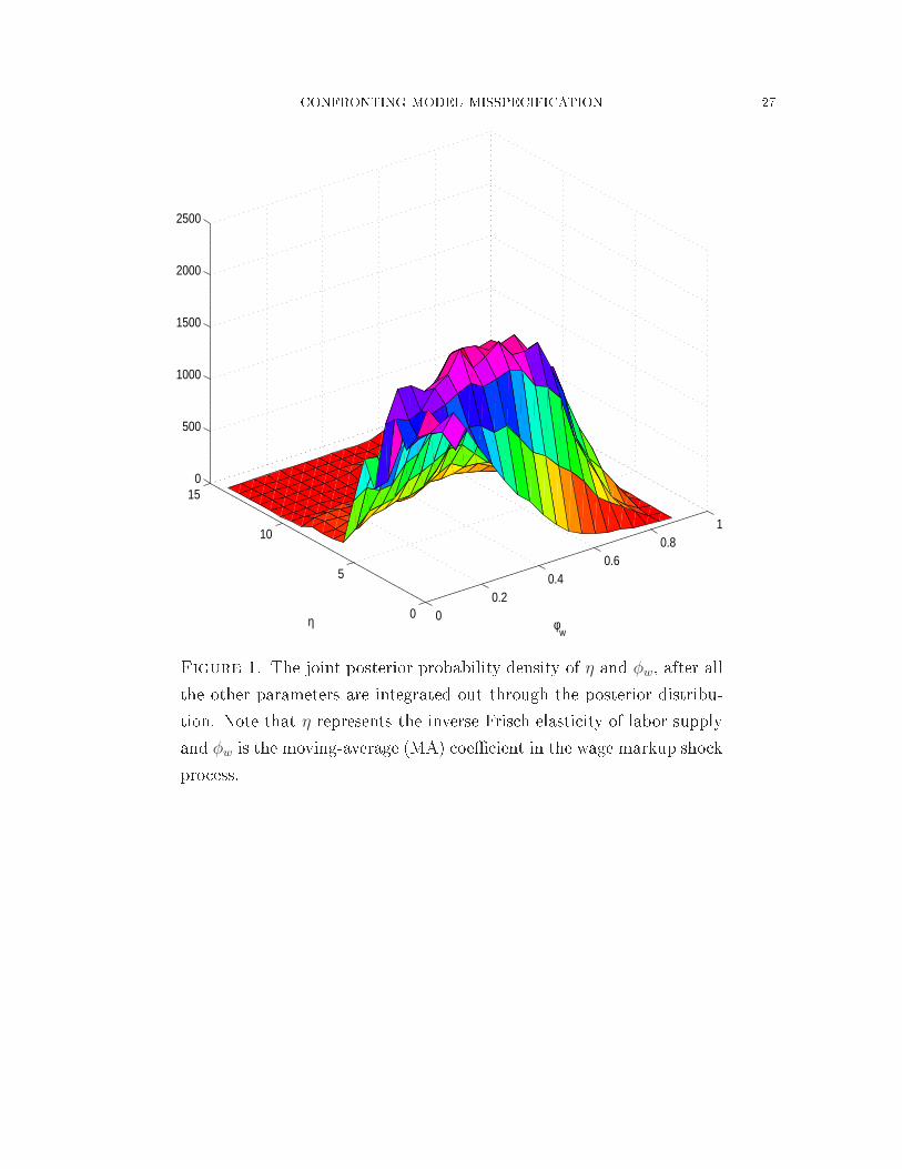
CONFRONTING MODEL MISSPECIFICATION 12The in�ation target (π∗) is another example in point. Our prior on this parameter isvery loose, overing the range from 1% to 8% for the annualized rates (Table 1). Themarginal posterior distribution for π∗ is very wide for both the DSGE model and forthe merged model, but the distribution for the merged shifts to the left and gives asubstantial probability (more than 45%) to the target below 4%.9 The estimate of the apital share α1 has in reased and the estimate of the labor share α2 has de reasedso that the sum α1 + α2 in the merged model is onsiderably smaller than that in theDSGE model, implying that this sour e of real rigidity is strong.Perhaps most notable hanges pertain to some persisten e parameters. As shown inTable 4, the 90% probability intervals for the parameters ρp, φp, and ρa are mu h widerin the merged model than in the DSGE model alone. The posterior distributions forpersisten e parameters tend to have a long fat tail toward zero, indi ating mu h moreun ertainty about the highly persistent sho k pro esses than the DSGE model wouldre ommend.Remember that a ombined number of parameters from the two models is very largeand the shape of the posterior probability density over this high-dimensional parameterspa e is extremely non-Gaussiann full of skewness and fat-tails. When we ompute themarginal 90% probability interval of one parameter by integrating out all the rest ofthe parameters, it is not un ommon that some posterior mode estimates fall outsidethe 90% probability intervals as indi ated in Tables 3 and 4. Take the two parametersη and φw as an example. The posterior-mode estimates of these two parameters areoutside the orresponding marginal 90% probability intervals. Figure 1 plots the two-dimensional joint probability density fun tion of η and φw. It an be seen from the�gure that the shape of this distribution has a mass probability density around theboundary de�ned by η = 0 and φw = 0 oupled with fat long tails. Sin e this two-dimensional probability density has already been marginalized by integrating out theother hundreds of parameters in the merged model, it gives us only a glimpse of the omplexity of the shape of the high-dimensional joint probability density, whi h isbeyond visualization.The resultant disagreement between the joint distribution and a marginal distribu-tion also shows up in the estimate and inferen e of q11, whi h measures the duration inwhi h the DSGE model dominates the BVAR model. The posterior-mode estimate ofq1,1 is outside the 90% probability interval and the marginal distribution of q11 is learly9Our sample overs the several high in�ation periods. The estimated target is mu h lower if we useonly the sample after 1987.

CONFRONTING MODEL MISSPECIFICATION 13skewed to the right. The estimate of q1,1 is 0.309, implying that the duration in whi hthe DSGE model dominates the BVAR model is about 1.5 quarters. As judged by the90% probability interval, the duration is unlikely to last for more than 3 quarters. Onthe other hand, the estimate of q2,2 is 0.72 and thus the most likely duration in whi hthe BVAR model dominates the DSGE model is about 3.5 quarters. The duration anlast as long as 7 quarters, as determined by the upper bound of the 90% interval (Table4).VI.3. A histori al perspe tive of the role of a model. The transition probability,qi,i, measures the average (un onditional) importan e of model i. Often one is inter-ested in knowing how important model i is at a parti ular time of the history. Figure2 displays the posterior probabilities of the DSGE model. Clearly, the DSGE model isoperative throughout the history, but for the most part, the probability of the DSGEmodel being near one lasts no more than one quarter at a time, onsistent with theestimate reported in Table 4. Moreover, the estimated DSGE model performs poorlyduring the re essions, as indi ated by the shaded bars in Figure 2.In ontrast, the probability of the BVAR model near one (i.e., the probability of theDSGE model near zero in Figure 2) tends to last for a few quarters at a time.The result that the DSGE model is operative sporadi ally throughout the history an be partially explained by Figure 3, whi h displays the log values of predi tivedensities of the merged model, the DSGE model, and the BVAR model. Clearly themerged model has higher predi tive densities than both the DSGE and BVAR modelsthroughout the entire history. The times when the predi tive density of the DSGEmodel is higher than the BVAR model are irregular and s attered without mu h dura-tion. Although the MDD for the DSGE model is mu h higher than the MDD for theBVAR model, the data prefers the DSGE model only intermittently throughout thesample.VI.4. Prior sensitivity. The MDD of a parti ular model is very sensitive to priorspe i� ations. In parti ular, the BVAR model has hundreds of parameters and theMDD varies wildly with di�erent priors. The �Minnesota-like� prior used in Smetsand Wouters (2007) ignores ross e�e ts among variables and the orrelation betweenthe onstant term and other oe� ients. Sims and Zha (1998) introdu es additionaldummy-observation omponents of the prior that in orporate orrelations in prior be-liefs about all oe� ients (in luding the onstant term) in every equation. Thus, themodel is pulled toward a form in whi h either all variables are stationary with means

CONFRONTING MODEL MISSPECIFICATION 14equal to the sample averages of the initial onditions or there are ointegration rela-tionships.The Sims and Zha (1998) prior has been found to improve out-of-sample fore astsin a variety of ontexts with e onomi time series. Indeed, when we use the exa tprior re ommended by Sims and Zha (1998), the log MDD of the BVAR is in reased to5894.6, as ompared to 5685.7 in Table 5. This MDD is about 150 in log value higherthan the DSGE ounterpart (Table 5). Given this stark fa t, one might on lude thatthe DSGE model must play no or little role in the merged model spa e. This on lusionwould be in orre t. The resultant merged model has the log value of MDD being inthe range from 6039.0 to 6044.4. The MDD of the merged model is mu h higher thanthe MDD of the BVAR, be ause the DSGE model ontinues to form an integral partof the model spa e in �tting the data. The posterior estimate of q1,1 rises to 0.473,while the posterior estimate of q2,2 rises to 0.833. Moreover, the posterior probabilitiesof the DSGE model throughout the history have a pattern similar to Figure 2.In general, when the prior spe i� ation for an individual model hanges, the MDD an hange drasti ally. But our extensive experiments indi ate that the merged modelpooling together the two models is insensitive to hanges in prior spe i� ations, in thesense that it dominates individual models by allowing both models to form an integralpart of the data generating pro ess.VII. E onomi impli ationsWe are now in a position to dis uss e onomi impli ations when one takes expli ita ount of both model un ertainty and parameter un ertainty in our merged frame-work.VII.1. Output �u tuations. A sho k to apital or investment, su h as a apitaldepre iation sho k, plays an important role in output �u tuations. Table 6 showsthat ontributions from the apital depre iation sho k a ount for lose to 50% of�u tuations in output in the short run (within two years) and about 40% of output�u tuations in the longer run (for three to �ve years). The DSGE model, if it istreated in isolation, would underestimate the magnitude of the ontributions from the apital depre iation sho k in output �u tuations. The underestimation is at least by10 per entage points for most fore ast horizons, as reported in Table 6.VII.2. Posterior distributions. Figure 4 displays the marginal posterior distribu-tions of four key stru tural parameters from the merged model (left hand olumn)

CONFRONTING MODEL MISSPECIFICATION 15and the DSGE model alone (right hand olumn). The posterior distributions fromthe merged model un over onsiderably more un ertainty about the parameters thanwhat is implied by the DSGE model alone. Moreover, the posterior distributions shift,giving more probability to the untrodden regions.• For the in�ation oe� ient in the Taylor rule (φπ), the merged model putsalmost zero probability on the value below 1.5 , while the DSGE model inisolation would put mass probability around 1.5 with a onsiderably tighter90% probability interval.

• For the Calvo pri e parameter (ξp), the posterior distribution from the mergedmodel shifts to the right, giving substantial probability to the values between0.6 and 0.8 as well as between 0.1 and 0.4.• For the Calvo wage parameter (ξw), the posterior distribution from the mergedmodel shifts to the left, giving onsiderable probability to the values betweenbetween 0.1 and 0.6, whereas the posterior distribution from the DSGE modelestimated in isolation on entrates around 0.4 with a mu h tighter 90% prob-ability interval.• For the parameter (S ′′) measuring investment adjustment osts, the posteriordistribution from the merged model spreads out to the values beyond 2, indi at-ing that the higher investment adjustment osts (between 2 and 4) is probable.Our estimates show that the estimation of the DSGE model utilizes roughly onethird of the data points in the sample. It is unsurprising that the error bands of DSGEparameters are wider for the merged model. What is new in our �ndings, however, isthat the error bands in the merged model are mu h more than 1.73 (a square root ofthree) times those when the DSGE model is estimated alone with all the data points.Figure 2 provides an insight of our �ndings. Sin e the DSGE model dominates theBVAR model only for the periods in whi h the data have more similarity than thedata in other periods, the data that experien e large �u tuations (as in the re essionperiods) are ex luded in the estimation of DSGE parameters. This ex lusion resultsin onsiderably more un ertainty about the estimates than what the number of datapoints would suggest.VII.3. Dynami responses. Figure 5 shows the impulse responses of output, on-sumption, real wage, and in�ation to a one-standard-deviation sho k to apital de-pre iation. The left hand olumn shows the responses generated from the estimatedmerged model and the right hand olumn shows the responses from the DSGE model

CONFRONTING MODEL MISSPECIFICATION 16when it is estimated in isolation. Comparing the two olumns side by side, one an seethe notable di�eren es between the merged model and the DSGE model.• Output responses in the merged model are very persistent, while the orre-sponding responses in the DSGE model alone return to the steady state aftertwo and a half years.• The magnitude of onsumption and real wage responses in the merged modelis onsiderably larger than that in the DSGE model when it is estimated sepa-rately.• A sho k to apital depre iation is a negative sho k to the apital sto k andthus the agent's wealth. As a result, onsumption falls due to the wealth e�e t,but the marginal ost of apital rises due to the de line in the apital sto k.When the DSGE model is estimated in isolation, the rise in the marginal ostof apital slightly dominates the fall in the real wage. Thus, the in rease inin�ation responses is signi� ant statisti ally but the magnitude is insigni� ante onomi ally. In the merged model, however, the fall in the real wage over-weighs the rise in the marginal ost of apital so that in�ation fall. In ontrastto the results generated from the DSGE model alone, in�ation responses arepredominantly negative in the short run (within the two years) before they risein the longer run (after the third year).Similar to the �ndings dis ussed in previous se tions, the error bands of impulse re-sponses in the merged model (left hand olumn in Figure 5) are onsiderably widerthan those generated by giving the DSGE model all the weight. These results empha-size the underlying un ertainty ignored by dis arding the BVAR model in the modelspa e. VIII. Con lusionWhen a parti ular model is usable for poli y pres riptions, e onomists understandthat the model is an approximation at best and should be used only with a grain of salt.A positive question is how to quantify the degree to whi h the model is misspe i�ed.Using a stru tural DSGE model and a redu ed-form BVAR model as an e onomi laboratory, we demonstrate that a merger of the two models exposes how misspe i�edboth models are. In parti ular, we show that even though the MDD for the DSGEmodel is mu h higher than the MDD for the BVAR model, the DSGE model dominatesthe BVAR model sporadi ally for only one third of the history. The estimated results

CONFRONTING MODEL MISSPECIFICATION 17from the merged model signi� antly alter the e onomi impli ations derived from theDSGE parameters and their impulse responses.The framework studied in this paper is general enough to be appli able to a varietyof e onomi questions beyond the parti ular appli ation used in this paper. One an,for example, study a stru tural BVAR model by identifying e onomi sho ks su h asa monetary poli y sho k, a redit sho k, an oil pri e sho k, and a te hnology sho k.One an then merge this stru tural BVAR model with the DSGE model that has thesame set of e onomi sho ks. The formal ommuni ation between these two stru turalmodels, fa ilitated by our framework, allows the resear her to re on ile the di�eren esbetween impulse responses implied by two isolated models when they are estimatedseparately. Moreover, the approa h explored in this paper allows for more than twomodels, and the models in luded in the merged framework need not be nested.Appendix A. Detailed data des riptionAll data are onstru ted from the original data in the Haver Analyti s Database.The onstru ted data, the original data identi�ers, and the data sour es are des ribedbelow.• Y Data

t = GDPHLN16N�USECON .• CData

t = (CN�USECON + CS�USECON - CSRU�USECON)∗100/JCXFE�USNALN16N�USECON .• IDatat = (CD�USECON + FNE�USECON)∗100/JCXFE�USNALN16N�USECON .• wData

t = LXNFC�USECON/100JCXFE�USNA .• πDatat = JCXFE�USNAtJCXFE�USNAt−1

.• LData

t = LXNFH�USECONLN16N�USECON .• FFRData

t = FFED�USECON400

.• QData

t = JCXFE�USNAGordonPri eCDplusES .LN16N�USECON: Civilian noninstitutional population: 16 years and over.Breaks in population are eliminated from 10-year ensuses and post 2000 Amer-i an Community Surveys using �error of losure� method. This fairly simplemethod was used by the Census Bureau to get a smooth population monthlypopulation series. This smooth series redu es the unusual in�uen e of drasti demographi hanges. Sour e: BLS.GDPH: Real gross domesti produ t (2005 dollars). Sour e: BEA.CN�USECON: Nominal personal onsumption expenditures: nondurable goods.Sour e: BEA.CS�USECON: Nominal onsumption expenditures: servi es. Sour e: BEA.

CONFRONTING MODEL MISSPECIFICATION 18CSRU�USECON: Nominal personal onsumption expenditures: housing andutilities. Sour e: BEA.CD�USECON: Nominal personal onsumption expenditures: durable goods.Sour e: BEA.FNE�USECON: Nominal private nonresidential investment: equipment & soft-ware. Sour e: BEA.JCXFE�USNA: PCE ex luding Food and Energy: Chain Pri e Index (2005=100).Sour e: BEA.LXNFC�USECON: Nonfarm business se tor: ompensation per hour (1992=100).Sour e: BLS.LXNFH�USECON: Nonfarm business se tor: hours of all persons (1992=100).Sour e: BLS.FFED�USECON: Nnnualized federal funds e�e tive rate. Sour e: FRB.GordonPri eCDplusES: Investment de�ator. The Tornquist pro edure is usedto onstru t this de�ator as a weighted aggregate index from the four quality-adjusted pri e indexes: private nonresidential stru tures investment, privateresidential investment, private nonresidential equipment & software investment,and personal onsumption expenditures on durable goods. Ea h pri e index is aweighted one from a number of individual pri e series within this ategories. Forea h individual pri e series from 1947 to 1983, we use Gordon (1990)'s quality-adjusted pri e index. Following Cummins and Violante (2002), we estimate ane onometri model of Gordon's pri e series as a fun tion of a time trend and afew NIPA indi ators (in luding the urrent and lagged values of the orrespond-ing NIPA pri e series); the estimated oe� ients are then used to extrapolatethe quality-adjusted pri e index for ea h individual pri e series for the samplefrom 1984 to 2007. These onstru ted pri e series are annual. Denton (1971)'smethod is used to interpolate these annual series on a quarterly frequen y. TheTornquist pro edure is then used to onstru t ea h quality-adjusted pri e indexfrom the appropriate interpolated quarterly pri e series.Appendix B. DSGE equilibrium dynami sWe introdu e the notation ∆xt = xt − xt−1. We use the hat variable, xt, to denotethe log deviation of the stationary variable Xt from its steady state value (i.e., xt =

log(Xt/X)). The log-linearized equilibrium onditions for our DSGE mode, below,summarize the equilibrium dynami s.

CONFRONTING MODEL MISSPECIFICATION 19πt − γpπt−1 =

κp

1 + αθp(µpt + mct) + βEt[πt+1 − γpπt], (pri e-Phillips urve) (A1)

wt − wt−1 + πt − γwπt−1 =κw

1 + ηθw(µwt + mrst − wt) +

βEt[wt+1 − wt + πt+1 − γwπt], (wage-Phillips urve) (A2)qkt = S′′λ2

I

{

∆it +1

1− α1

(∆qt + α2∆zt)

−βEt

[

∆it+1 +1

1− α1

(∆qt+1 + α2∆zt+1)

]}

, (investment de ision) (A3)qkt = Et

{

∆at+1 +∆Uc,t+1 −1

1− α1

[α2∆zt+1 +∆qt+1]

+β

λI

[

(1− δ)qk,t+1 − δδt+1 + rk rk,t+1

]

}

, ( apital de ision) (A4)rkt = σuut, ( apa ity utilization) (A5)0 = Et

[

∆at+1 +∆Uc,t+1

−1

1− α1

[α2∆zt+1 + α1∆qt+1] + Rt − πt+1

]

, (bond de ision) (A6)kt =

1− δ

λI

[

kt−1 −1

1− α1

(α2∆zt +∆qt)

]

−δ

λI

δt +

(

1−1− δ

λI

)

it, ( apital law of motion) (A7)yt = cy ct + iy it + uyut + gygt, (resour e onstraint) (A8)yt = α1

[

kt−1 + ut −1

1− α1

(α2∆zt +∆qt)

]

+ α2 lt, (produ tion fun tion) (A9)wt = rkt + kt−1 + ut −

1

1− α1

(α2∆zt +∆qt)− lt, (labor & apital demand)(A10)Rt = ρrRt−1 + (1 − ρr) [φππt + φy yt] + σrεrt, (interest rate rule) (A11)where

mct =1

α1 + α2

[α1rkt + α2wt] + αyt, (A12)mrst = ηlt − Uct, (A13)Uct =

βb(1− ρa)

λ∗ − βbat −

λ∗

(λ∗ − b)(λ∗ − βb)[λ∗ct − b(ct−1 −∆λ∗

t )]

+βb

(λ∗ − b)(λ∗ − βb)[λ∗Et(ct+1 +∆λ∗

t+1)− bct], (A14)Note that πt is in�ation, wt is real wage, qkt is the shadow pri e of existing apital(Tobin's q), it is investment, qt is the biased te hnology sho k pro ess, zt is the neutralte hnology sho k pro ess, at is the risk premium (preferen e) sho k pro ess, ut isthe utilization rate of apital, rkt is the real rental pri e of apital, δt is the apital

CONFRONTING MODEL MISSPECIFICATION 20depre iation sho k pro ess, Rt is the nominal rate of interest, kt is the apital sto k,yt is output, ct is onsumption, gt is government spending, and lt is hours worked.The steady-state variables are given by

rk =λI

β− (1 − δ), (A15)

uy ≡rkK

Y λI

=α1

µp

, (A16)iy = [λI − (1− δ)]

α1

µprk, (A17)

cy = 1− iy − gy. (A18)The new parameters introdu ed in the above equilibrium onditions areλI = (λqλ

α2

z )1

1−α1 ,

λ∗ = (λα2

z λα1

q )1

1−α1 ,

∆λ∗

t =1

1− α1

(α1∆qt + α2∆zt),

θp =µp

µp − 1,

κp =(1− βξp)(1 − ξp)

ξp,

α =1− α1 − α2

α1 + α2

,

θw ≡µw

µw − 1,

κw =(1 − βξw)(1 − ξw)

ξw.Note that gy is the average ratio of government spending to output, cy is the averageratio of onsumption to output, iy is the average ratio of investment to output, µpt isthe average pri e markup, µwt is the average wage markup, λq is the growth rate ofinvestment-spe i� te hnology, λz is the growth rate of neutral te hnology, α1 is the ost share of apital input, α2 is the ost share of labor input, δ is the average apitaldepre iation rate, b is internal habit, S ′′ represents the investment adjustment osts,

σu represents the urvature of the ost fun tion of variable apital utilization, ξp isthe probability that a �rm annot adjust its pri e, γp measures the degree of pri eindexation, ξw is a fra tion of households who annot reoptimize their wage de isions,and γw measures the degree of wage indexation.In addition to all the equilibrium onditions, we have 7 sho k pro esses:logµwt = (1− ρw) logµw + ρw logµw,t−1 + σwεwt − φwσwεw,t−1, (pri e markup)logµpt = (1− ρp) logµp + ρp logµp,t−1 + σpεpt − φpσpεp,t−1, (wage markup)

log zt = (1− ρz) log z + ρz log zt−1 + σzεzt, (neutral te hnology)

CONFRONTING MODEL MISSPECIFICATION 21log qt = (1− ρq) log q + ρq log qt−1 + σqεqt, (embodied te hnology)

logAt = (1 − ρa) logA+ ρa logAt−1 + σaεat, (risk premium)log δt = (1− ρd) log δ + ρd log δt−1 + σdεdt, ( apital depre iation)

log Gt = (1 − ρg) log G+ ρg log Gt−1 + σgεgt + ρgzσzεzt, (spending)where ε represents an i.i.d. normal sho k and σ represents the orresponding standarddeviation.To ompute the equilibrium, we eliminate both ut and rkt by using (A5) and (A8),leaving 9 equations and 9 variables πt, wt, it, qkt, ct, kt, yt, lt, and Rt. Out of these9 variables, we have 7 orresponding observable variables (ex ept qkt and kt) for ourestimation. Finally, we have one additional observable variable, the biased te hnologysho k qt, used in our estimation.In addition to the 9 equilibrium onditions, we have 7 equations des ribing the ARpro esses for the 7 stru tural sho ks, 4 equations des ribing the 2 MA pro esses, and7 equations on erning the 7 expe tational terms in the system. Thus, there are 27DSGE equations in total.

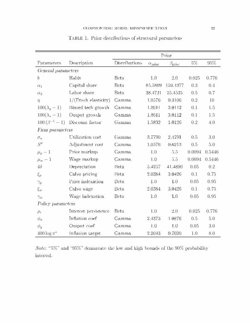
CONFRONTING MODEL MISSPECIFICATION 22Table 1. Prior distributions of stru tural parametersPriorParameters Des ription Distributions αprior βprior 5% 95%General parametersb Habit Beta 1.0 2.0 0.025 0.776

α1 Capital share Beta 85.5869 159.4377 0.3 0.4

α2 Labor share Beta 38.4721 25.4535 0.5 0.7

η 1/(Fris h elasti ity) Gamma 1.0576 0.3106 0.2 10

100(λq − 1) Biased te h growth Gamma 1.8611 3.0112 0.1 1.5

100(λ∗ − 1) Output growth Gamma 1.8611 3.0112 0.1 1.5

100 (β−1 − 1) Dis ount fa tor Gamma 1.5832 1.0126 0.2 4.0Firm parametersσu Utilization ost Gamma 3.7790 2.4791 0.5 3.0

S ′′ Adjustment ost Gamma 1.0576 0.6213 0.5 5.0

µp − 1 Pri e markup Gamma 1.0 5.5 0.0094 0.5446

µw − 1 Wage markup Gamma 1.0 5.5 0.0094 0.5446

4δ Depre iation Beta 5.4257 41.4890 0.05 0.2

ξp Calvo pri ing Beta 2.0384 3.0426 0.1 0.75

γp Pri e indexation Beta 1.0 1.0 0.05 0.95

ξw Calvo wage Beta 2.0384 3.0426 0.1 0.75

γw Wage indexation Beta 1.0 1.0 0.05 0.95Poli y parametersρr Interest persisten e Beta 1.0 2.0 0.025 0.776

φπ In�ation oef Gamma 2.4373 1.0876 0.5 5.0

φy Output oef Gamma 1.0 1.0 0.05 3.0

400 logπ∗ In�ation target Gamma 2.9043 0.7690 1.0 8.0Note: �5%� and �95%� demar ate the low and high bounds of the 90% probabilityinterval.

CONFRONTING MODEL MISSPECIFICATION 23Table 2. Prior distributions of sho k parametersPriorParameters Des ription Distributions αprior βprior 5% 95%Persisten e parametersρp Pri e markup AR Beta 1.0 2.0 0.025 0.776

φp Pri e markup MA Beta 1.0 2.0 0.025 0.776

ρw Wage markup AR Beta 1.0 2.0 0.025 0.776

φw Wage markup MA Beta 1.0 2.0 0.025 0.776

ρgz Spending on te h Gamma 1.8611 1.5056 0.2 3.0

ρa Preferen e Beta 1.0 2.0 0.025 0.776

ρq Biased te h Beta 1.0 1.0 0.05 0.95

ρz Neutral te h Beta 1.0 1.0 0.05 0.95

ρd Depre iation Beta 1.0 2.0 0.025 0.776Standard deviationsσr Monetary poli y Inverse Gamma 0.4436 0.0009 0.0005 1.0

σp Pri e markup Inverse Gamma 0.4436 0.0009 0.0005 1.0

σw Wage markup Inverse Gamma 0.4436 0.0009 0.0005 1.0

σg Gov spending Inverse Gamma 0.4436 0.0009 0.0005 1.0

σz Neutral te h Inverse Gamma 0.4436 0.0009 0.0005 1.0

σa Preferen e Inverse Gamma 0.4436 0.0009 0.0005 1.0

σq Biased te h Inverse Gamma 0.4436 0.0009 0.0005 1.0

σd Depre iation Inverse Gamma 0.4436 0.0009 0.0005 1.0Transition matrix parametersq11 DSGE model Diri hlet 5.6667 1.0 0.5905 0.9911

q22 BVAR model Diri hlet 5.6667 1.0 0.5905 0.9911Note: �5%� and �95%� demar ate the low and high bounds of the 90% probabilityinterval.

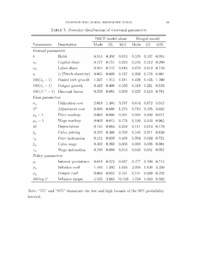
CONFRONTING MODEL MISSPECIFICATION 24Table 3. Posterior distributions of stru tural parametersDSGE model alone Merged modelParameters Des ription Mode 5% 95% Mode 5% 95%General parametersb Habit 0.544 0.493 0.624 0.528 0.597 0.954α1 Capital share 0.177 0.151 0.203 0.250 0.212 0.290α2 Labor share 0.804 0.747 0.818 0.679 0.614 0.740η 1/(Fris h elasti ity) 0.005 0.003 0.167 0.399 0.578 6.801100(λq − 1) Biased te h growth 1.507 1.215 1.911 1.438 1.145 1.700100(λ∗ − 1) Output growth 0.483 0.400 0.569 0.519 0.221 0.576100 (β−1 − 1) Dis ount fa tor 0.228 0.081 0.909 0.222 0.113 0.781Firm parametersσu Utilization ost 2.018 1.404 3.787 0.654 0.672 3.947S ′′ Adjustment ost 0.800 0.608 1.278 0.710 0.495 3.032µp − 1 Pri e markup 0.000 0.000 0.001 0.000 0.000 0.017µw − 1 Wage markup 0.003 0.015 0.176 0.109 0.043 0.9654δ Depre iation 0.145 0.064 0.204 0.111 0.013 0.170ξp Calvo pri ing 0.372 0.308 0.760 0.540 0.211 0.839γp Pri e indexation 0.121 0.028 0.408 0.394 0.024 0.721ξw Calvo wage 0.303 0.269 0.606 0.069 0.096 0.604γw Wage indexation 0.790 0.088 0.954 0.040 0.081 0.957Poli y parametersρr Interest persisten e 0.618 0.572 0.687 0.477 0.490 0.744φπ In�ation oef 1.480 1.392 1.693 2.008 1.820 3.230φy Output oef 0.066 0.052 0.101 0.141 0.099 0.228400 log π∗ In�ation target 5.576 3.863 10.109 5.764 1.693 8.583Note: �5%� and �95%� demar ate the low and high bounds of the 90% probabilityinterval.

CONFRONTING MODEL MISSPECIFICATION 25Table 4. Posterior distributions of sho k parametersDSGE model alone Merged modelParameters Des ription Mode 5% 95% Mode 5% 95%Persisten e parametersρp Pri e markup AR 0.786 0.587 0.878 0.188 0.037 0.972φp Pri e markup MA 0.627 0.276 0.820 0.168 0.060 0.802ρw Wage markup AR 0.992 0.987 0.997 0.990 0.815 0.988φw Wage markup MA 0.530 0.305 0.827 0.000 0.040 0.695ρgz Spending on te h 0.947 0.490 1.348 1.690 0.490 2.138ρa Preferen e 0.988 0.973 0.995 0.988 0.242 0.953ρq Biased te h 0.994 0.988 0.997 0.989 0.971 0.993ρz Neutral te h 0.942 0.927 0.961 0.903 0.910 0.989ρd Depre iation 0.915 0.854 0.975 0.888 0.869 0.990Standard deviationsσr Monetary poli y 0.003 0.002 0.003 0.002 0.002 0.003σp Pri e markup 1.012 0.593 2.109 1.348 0.014 1.095σw Wage markup 0.023 0.017 0.065 0.009 0.016 0.404σg Gov spending 0.029 0.026 0.031 0.023 0.022 0.033σz Neutral te h 0.008 0.007 0.009 0.007 0.007 0.010σa Preferen e 0.061 0.035 0.137 0.030 0.013 0.075σq Biased te h 0.006 0.006 0.007 0.004 0.004 0.007σd Depre iation 0.096 0.065 0.261 0.098 0.069 1.008Transition matrix parametersq1,1 DSGE model 0.309 0.415 0.684q2,2 BVAR model 0.720 0.689 0.861Note: �5%� and �95%� demar ate the low and high bounds of the 90% probabilityinterval.

CONFRONTING MODEL MISSPECIFICATION 26Table 5. Marginal data densitiesMerged model DSGE BVAR5848.90 - 5854.03 5735.49 - 5736.39 5685.74Table 6. Output varian e de ompositions: ontributions from a apitaldepre iation sho k (%)Quarters 4 8 12 16 20Merged 48.60 47.89 43.77 40.54 38.58DSGE alone 39.75 35.91 30.18 27.41 26.25

CONFRONTING MODEL MISSPECIFICATION 27

00.2

0.40.6

0.81

0

5

10

150

500

1000

1500

2000

2500

φw

ηFigure 1. The joint posterior probability density of η and φw, after allthe other parameters are integrated out through the posterior distribu-tion. Note that η represents the inverse Fris h elasti ity of labor supplyand φw is the moving-average (MA) oe� ient in the wage markup sho kpro ess.

CONFRONTING MODEL MISSPECIFICATION 28

1965 1970 1975 1980 1985 1990 1995 2000 2005 20100

0.1

0.2

0.3

0.4

0.5

0.6

0.7

0.8

0.9

1Sm

ooth

ed p

roba

bilit

ies

of th

e D

SGE

mod

el

Figure 2. The posterior probabilities that the DSGE model is sele tedby the data. The shaded bars mark the NBER re ession dates.

CONFRONTING MODEL MISSPECIFICATION 29

19

60

19

65

19

70

19

75

19

80

19

85

19

90

19

95

20

00

20

05

20

10

−6

0

−5

0

−4

0

−3

0

−2

0

−1

00

10

20

30

40

Log predictive densities

DS

GE

BV

AR

Me

rge

d

Figure 3. Log values of predi tive densities from the three models.

CONFRONTING MODEL MISSPECIFICATION 301 2 3 4

0

1

2

3

4

5Merged model

Inflation coefficient in Taylor rule1 2 3 4

0

1

2

3

4

5DSGE model alone

Inflation coefficient in Taylor rule

0 0.2 0.4 0.6 0.8 10

1

2

3

4

Price stickness parameter0 0.2 0.4 0.6 0.8 1

0

1

2

3

4

Price stickness parameter

0 0.2 0.4 0.6 0.8 10

1

2

3

4

5

Wage stickness parameter0 0.2 0.4 0.6 0.8 1

0

1

2

3

4

5

Wage stickness parameter

0 1 2 3 4 50

1

2

3

Investment adjustment costs0 1 2 3 4 5

0

1

2

3

Investment adjustment costsFigure 4. Marginal posterior distributions of some key stru tural pa-rameters for the merged model (left olumn) and for the DSGE modelwhen it is estimated in isolation (right olumn).

CONFRONTING MODEL MISSPECIFICATION 31−10

−5

0

x 10−3 Merged model

Ou

tpu

t

DSGE model alone

−10

−5

0

x 10−3

Co

nsu

mp

tio

n

−14−12−10

−8−6−4−2

x 10−3

Re

al w

ag

e

4 8 12 16

−1

−0.5

0

0.5

1x 10

−3

Infla

tio

n

Quarters4 8 12 16

QuartersFigure 5. Impulse responses to a apital depre iation sho k for themerged model (left olumn) and for the DSGE model when estimatedin isolation (right olumn). The shaded area represents 90% posteriorprobability bands and the thi k line represents the median estimate.

CONFRONTING MODEL MISSPECIFICATION 32Referen esAltig, D., L. J. Christiano, M. Ei henbaum, and J. Linde (2004): �Firm-Spe i� Capital, Nominal Rigidities and the Business Cy le,� Federal Reserve Bankof Cleveland Working Paper 04-16.Bro k, W. A., S. N. Durlauf, and K. D. West (2003): �Poli y Evaluation inUn ertain E onomi Environment,� Brookings Papers on E onomi A tivity, 1, 235�301.Chari, V., P. J. Kehoe, and E. R. M Grattan (2000): �Sti ky Pri e Models ofthe Business Cy le: Can the Contra t Multiplier Solve the Persisten e Problem?,�E onometri a, 68(5), 1151�1180.Cogley, T., and T. J. Sargent (2005): �The Conquest of U.S. In�ation: Learningand Robustness to Model Un ertainty,� Review of E onomi Dynami s, 8, 528�563.Cummins, J. G., and G. L. Violante (2002): �Investment-Spe i� Te hni al Changein the United States (1947-2000): Measurement and Ma roe onomi Consequen es,�Review of E onomi Dynami s, 5, 243�284.Del Negro, M., and F. S horfheide (2004): �Priors from General EquilibriumModels for VARs,� International E onomi Review, 45, 643�673.(2008): �Forming Priors for DSGE Models (and How It A�e ts the Assess-ment of Nominal Rigidities),� Manus ript, Federal Reserve Bank of New York andUniversity of Pennsylvania.Denton, F. T. (1971): �Adjustment of Monthly or Quarterly Series to Annual Totals:An Approa h Based on Quadrati Minimization,� Journal of the Ameri an Statisti alAsso iation, 66, 99�102.Diebold, F. X. (1991): �A Note on Bayesian Fore ast Combination Pro edures,� inE onomi Stru tural Change: Analysis and Fore asting, ed. by A. H. Westlund, andP. Ha kl, pp. 225�232. Springer-Verlag, New York, NY.Fisher, M., and D. F. Waggoner (2010): �Mixture Models and Bayesian ModelSele tion,� Unpublished manus ript.Geweke, J., and G. Amisano (forth oming): �Optimal Predi tion Pools,� Journalof E onometri s.Gordon, R. J. (1990): The Measurement of Durable Goods Pri es. University ofChi ago Press, Chi ago,Illinois.Hansen, L. P., and T. J. Sargent (2001): �A knowledging Misspe i� ation inMa roe onomi Theory,� Review of E onomi Dynami s, 4, 519�535.

CONFRONTING MODEL MISSPECIFICATION 33Liu, Z., D. F. Waggoner, and T. Zha (2010): �Sour es of Ma roe onomi Flu tu-ations: A Regime-Swit hing DSGE Approa h,� Unpublished manus ript.Sims, C. A. (2003): �Probability Models for Monetary Poli y De isions,� Manus ript,Prin eton University.Sims, C. A., D. F. Waggoner, and T. Zha (2008): �Methods for Inferen ein Large Multiple-Equation Markov-Swit hing Models,� Journal of E onometri s,146(2), 255�274.Sims, C. A., and T. Zha (1998): �Bayesian Methods for Dynami Multivariate Mod-els,� International E onomi Review, 39(4), 949�968.Smets, F., and R. Wouters (2007): �Sho ks and Fri tions in US Business Cy les:A Bayesian DSGE Approa h,� Ameri an E onomi Review, 97, 586�606.West, M., and J. Harrison (1997): Bayesian Fore asting and Dynami Models.Springer, 2nd edn.Federal Reserve Bank of Atlanta, Federal Reserve Bank of Atlanta and EmoryUniversity