
OntheFluidMechanicsofPartialDewatering ...7319/FULLTEXT01.pdf ·...
81
On the Fluid Mechanics of Partial Dewatering during Roll Forming in Paper Making by Richard Holm May 2002 Technical Reports from Royal Institute of Technology Department of Mechanics Fax´ enLaboratoriet S-100 44 Stockholm, Sweden
Transcript of OntheFluidMechanicsofPartialDewatering ...7319/FULLTEXT01.pdf ·...
On the Fluid Mechanics of Partial Dewatering
during Roll Forming in Paper Making
by
Richard Holm
May 2002Technical Reports from
Royal Institute of TechnologyDepartment of Mechanics
FaxenLaboratorietS-100 44 Stockholm, Sweden

Akademisk avhandling som med tillstand av Kungliga Tekniska Hogskolani Stockholm framlagges till offentlig granskning for avlaggande av teknolo-gie licentiatexamen fredagen den 14:e juni 2002 kl 13.00 i seminarierum 40,Teknikringen 8, KTH, Valhallavagen 79, Stockholm.
c©Richard Holm 2002
Universitetsservice US AB, Stockholm 2002

R. Holm 2002 On the Fluid Mechanics of Partial Dewatering during Roll Form-ing in Paper Making.
Department of Mechanics, FaxenLaboratoriet Royal Institute of TechnologyS-100 44 Stockholm, Sweden
Abstract
The present work deals with some aspects of the fluid mechanics of paper-making, more specifically partial dewatering during roll forming. The studyis mainly experimental. Pressure and wire position measurements have beencarried out in an experimental facility, the KTH-Former, which models the rollforming zone of a paper machine.
Measurements are carried out with pure water for three different wires (fab-rics): A non-permeable, a semi-permeable and a conventional wire. Althoughnot used in paper making, the non-permeable wire is useful when trying tounderstand the fundamental mechanics of roll forming. The semi-permeablewire with finite but low permeability is used to model the effects of the fibreweb on the drainage.
Tests have mainly been carried out for different wire tensions and differentjet speeds. It is shown that the local curvature of the wire is strongly correlatedto the dewatering pressure.
The conventional wire shows a single pressure peak causing complete de-watering in the first part of the dewatering zone. The pressure distributions forthe non- and semi-permeable wires are found to show two consecutive pressurepeaks followed by a suction peak where the wire is taken off the roll. Thisoscillating behaviour is due to capillary waves where the wire tension plays therole of surface tension on a free surface. The wavy behaviour of the wire is re-covered from an analytical model and the effect is governed by a dimensionlessWeber number. The measured wave lengths correspond well to those given bythe theory.
When the wire tension is high, i.e. a high dewatering pressure, the flow inthe impingement region collapses when the dynamic pressure of the headboxjet is about half of the dewatering pressure.
It is shown experimentally that the local drainage shows a correlation tothe dewatering pressure and hence to the wire curvature.
Descriptors: Fluid mechanics, roll forming, partial dewatering, capillarywaves


Contents
Chapter 1. Introduction 11.1. The paper machine 11.2. Roll forming studies 4
Chapter 2. Experimental setup 112.1. The KTH-Former 112.2. Headbox contraction 202.3. Measurement techniques 222.4. Data acquisition 33
Chapter 3. Theoretical considerations of roll forming 353.1. Dimensional analysis 353.2. The relation between curvature and pressure 363.3. Wire curvature in cylindrical coordinates 373.4. Roll forming theory 39
Chapter 4. Results 454.1. Overview of pressure and wire position 454.2. Detailed study of pressure and wire position 534.3. Local drainage measurements 61
Chapter 5. Discussion and summary 655.1. Wire curvature and pressure signature 655.2. Consistency of pressure and wire position data 675.3. A comment on the drainage data 695.4. The wire oscillatory behaviour 705.5. Summary 71
Acknowledgements 73
References 75
v
CHAPTER 1
Introduction
Fluid mechanics is a basic scientific as well as an applied and engineering sub-ject with applications in many different fields, such as aeronautics, energy con-version, geophysics, biomedical flows, chemical engineering, paper technologyetc. For some applications fluid mechanics is the basic topic (such as aircraftengineering), in others fluid mechanics is one of several important factors.
The present work deals with some aspects of the fluid dynamics of paper-making, namely the initial dewatering during roll forming. The study is mainlyexperimental, using a model of the roll forming section of a paper machine. Theexperiments presented use water without fibres, and is therefore restricted tostudy the fundamental dynamics of the water jet and wire during roll formingand not the forming of the paper itself. However, it is argued that the dynamicsare similar with and without fibres. The present chapters are arranged to firstgive a brief description of paper making and modern paper making machines,thereafter give a survey of relevant literature concerning roll forming and alsosome discussion about the parameters which may affect the flow in the rolldewatering zone.
1.1. The paper machine
The history of paper making originates in China more than 2000 years ago.At that time single paper sheets were handmade, whereas today a modernhigh producing paper machine can produce up to 600 000 ton/year. The ba-sic principle of a paper machine is, however, still the same. It starts with afibre suspension with low concentration of cellulose fibres in water, followed bydewatering on a permeable weave (forming fabric or wire) and it ends with apress and a drying section. A schematic picture of the paper making process isseen in figure 1.1. The process of suspension feeding and dewatering is usuallycalled forming, meaning the forming of the fibre web, which is the critical stageof building up the paper sheet.
In its simplest way, similar to the early days of paper making, the dewa-tering is caused by gravity on a horizontally held wire, a so called Fourdrinierformer. A development of this was to introduce forced dewatering by localsuction below the wire and finally enclose the suspension between two wires
1

2 1. INTRODUCTION
and have two-sided dewatering, a so called twin-wire former or gap former.This shows some great advantages on the stability of the fibre suspension andmakes it possible to increase the production speed compared to the Fourdrinierformer. The forced dewatering mechanism is due to the deflection of the wire-web-wire sandwich over a roll and/or over deflector blades. A perforated rollwith low pressure inside the roll is used to obtain two-sided dewatering (twin-wire forming). Twin-wire forming shows approximately a fourfold dewateringcapacity and a more symmetric paper sheet with improved formation (i.e. amore homogeneous fibre distribution). Combinations of Fourdrinier and gapforming and also a combination of twin-wire roll and blade dewatering followedby suction boxes are used in some new production units. The variety of designsis partly due to the ambition to influence the forming of the web during dewa-tering in order to optimise different properties of the paper. There is a numberof different designs of twin wire forming machines, where roll forming usually,but not always, is part of the forming section. For an overview of differentdesigns see Malashenko & Karlsson (2000).
Paper is not a well-defined product, it includes board with a surface densityof 200-400 g/m2 (grammage) as well as newsprint with a grammage 40-50 g/m2
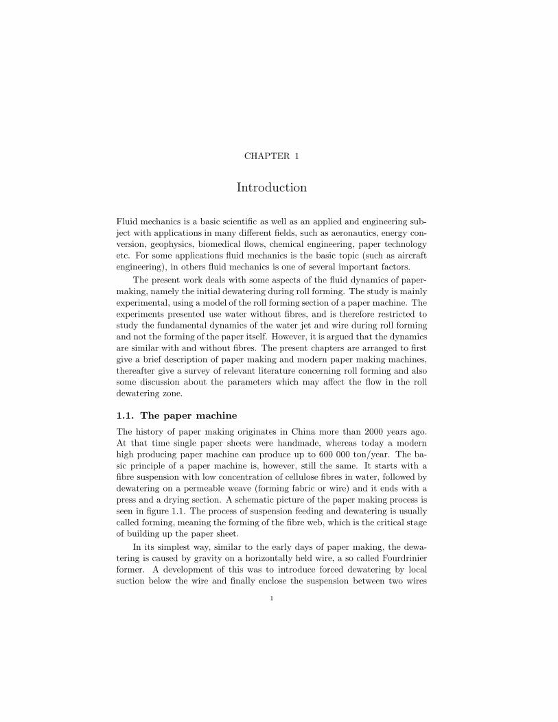
and also many other types of qualities for various applications. The productionspeed of a board machine is of the order of 400 m/min whereas a newsprintmachine could reach as high as 1800 m/min. For both these cases similar roll-blade forming techniques are applied even though board is manufactured inseveral layers. A roll-blade former design is shown in figure 1.2 which is foundin the EuroFEX pilot machine at STFI, Stockholm. Also for tissue making(14-25 g/m2) roll forming is used, but in that case with one-sided dewatering,using a solid forming roll.
Figure 1.1. The paper making process from pulp to paper sheet
A modern paper production unit consists of a forming section, the follow-ing press and drying section, see figure 1.1. In the forming section, the fibresuspension is fed into the headbox from the supporting system of pumps andpipes. The headbox consists of three parts, a flow distributor, a tube packageand a contraction. The flow distributor should provide a constant flow per unit
1.1. THE PAPER MACHINE 3
Forming roll
Five fixed blades
Six movable blades withblade forces F
Headbox
Variable wrap angle
Figure 1.2. The STFI-Former, combined roll and blade former
width into the headbox and is designed for a constant pressure across the head-box width. This is followed by the tube package where flow rate differences willbe reduced due to the pressure drop across it. The area is abruptly increasedin steps through this part, therefore it is also known as a step diffusor package,which will result in high turbulence levels and ideally a homogeneous velocityprofile at the outlet of the diffusers. The step diffusers end in the contractionwhere the flow speed increases and finally leaves the nozzle as a free plane jetwith a thickness of the order of 10 mm. In the contraction so called vanesmay be used, in order to control the fibre orientation and/or separate differentfibre layers. The flow motion in the contraction was the subject of the doc-toral thesis by Parsheh (2001), who studied the turbulence development, theboundary layers along the vanes as well as the wakes downstream of the vanes.The work covered both experimental and numerical studies of the problem andgave useful information for further studies.
When the fibre suspension leaves the headbox it is in the form of an ideallytwo-dimensional plane jet, typically one centimeter thick and up to 10 m wide.This jet impinges on the wire at a small angle, usually almost tangential to thewire, about 20 cm downstream of the headbox nozzle outlet. The hydrodynam-ics of the plane jet was thoroughly studied by Soderberg (1999). He determinedthe stability of a plane jet both experimentally and theoretically and showedthat the jet is susceptible to two-dimensional sinuous wave disturbances. In hisexperiments he could observe the breakdown of the waves, and that this may
4 1. INTRODUCTION
result in longitudinal (streaky) structures in the jet. Streaky structures canalso be found in the final paper sheet and Soderberg proposed that the reasonfor streaks found in the paper is because of a the streaks observed inside thejet.
At the impingement, the jet speed is close to the wire speed but a differencemay be intentionally set in a real paper machine, so called rush or drag relatedto the wire speed, in order to control the forming. In a Fourdriner formerthe dewatering starts immediately and continues until the web is taken off theforming wire to a press felt. In twin-wire forming the wire-web-wire sandwichwill be deflected to generate a dewatering pressure. After the forming sectionthe fibre distribution is practically frozen, although the surface structure maybe changed in the later press and drying sections, e.g. in the shoe press nipand calander rolls.
In a paper machine the cellulose fibres are initially in a dilute suspension (ofthe order of one percent by weight). However even under such conditions thefibres tend to entangle mechanically to form clusters, so called fibre flocs. Thisis an unwanted property, since the fibre flocs may give rise to a inhomogeneouspaper. The fibre flocs may to some extent be affected by the design of the flowdistributor, tube package and contraction.
The natural fibre adhesion, due to hydrogen bonding, is the primary groundfor the build up of the paper strength. Additional fillers (clay or chalk) can bemixed into the fibre suspension to control properties like opacity and surfacestructure of the paper. Retention aid chemicals are used to catch the fillerparticles in the fibre web during dewatering. The structure and the strengthof the paper is related to the fibre orientation. The fibre orientation is affectedby the shear flow in the headbox and also during the dewatering. Anotherimportant aspect of forming is that flocculation should be reduced as much aspossible in order to achieve an evenly distributed fibre mat with the requestedproperties of the final paper product.
1.2. Roll forming studies
Since the introduction of roll forming and due to the request to optimise theprocess, the understanding of this dewatering stage has been of special interest.The principle of roll forming is that when the fibre suspension is between theroll and an outer wire there is a pressure build-up (dewatering pressure) whichforces the water through the wire. The dewatering pressure p is generallydescribed by relation (1.1)
p =T
R(1.1)
where T is the outer wire tension and R is the roll (or wire) radius.
1.2. ROLL FORMING STUDIES 5
Equation (1.1) means that the dewatering pressure is constant along thewrap length of the wire. However, the wire is flexible which means that itsposition is not known a priori. In order to understand the dynamics of rollforming the determination of the wire position is therefore crucial. One shouldalso point out that for blade forming similar arguments are relevant. In orderto understand the dewatering process the wire geometry has to be known.
One of the early studies of roll forming is the one by Wahren et al. (1975).They carried out some measurements of the pressure on the forming roll, byhaving a flush-mounted pressure transducer mounted in the roll wall sensing thepressure at the roll surface. Their data showed a rapid increase in the pressureup to a a fairly constant level which was slightly below the T/R-value. Theyalso tried to analyse their data through a control volume approach using theirmeasured pressure data as boundary conditions. In this way they presentedresults concerning both the drainage and the wire position.
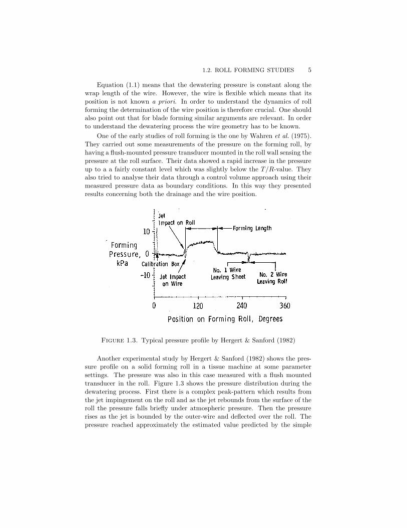
Figure 1.3. Typical pressure profile by Hergert & Sanford (1982)
Another experimental study by Hergert & Sanford (1982) shows the pres-sure profile on a solid forming roll in a tissue machine at some parametersettings. The pressure was also in this case measured with a flush mountedtransducer in the roll. Figure 1.3 shows the pressure distribution during thedewatering process. First there is a complex peak-pattern which results fromthe jet impingement on the roll and as the jet rebounds from the surface of theroll the pressure falls briefly under atmospheric pressure. Then the pressurerises as the jet is bounded by the outer-wire and deflected over the roll. Thepressure reached approximately the estimated value predicted by the simple

6 1. INTRODUCTION
model (T/R, see equation (1.1)) and remained at this level for 85 degrees fol-lowed by a pressure decrease to zero. In the remaining part of the roll wraplength the pressure is zero which indicates a complete dewatering. Finally, atwire separation at 180 degrees from initial jet impingement, a suction peak isseen in the pressure which is due to the wire leaving the roll. From the pressuredistribution the actual forming length was determined by means of the part ofhigh pressure. They also changed the wire tension and it was shown that thedewatering length decreased with increasing wire tension and that the maxi-mum dewatering pressure seems to scale with the wire tension. They also triedvarious jet impingement angles which gives slightly different pressure signature,especially near the impingement region. All in all the pressure profile obtainedby Hergert & Sanford are similar to those of Wahren et al. (1975) and seem tobe characteristic for cases with complete dewatering.
The pressure profiles are different in the case of only partial dewateringduring the roll forming stage. This is pointed out by Malashenko & Karlsson(2000) and is shown in figure 1.4. Initially there is a pressure build up as in theprevious studies, however when reaching the plateau, there is an oscillation inthe pressure before an intense negative pressure pulse at the point of separationof the wire from the roll.
Figure 1.4. A pressure profile in the case of partial dewater-ing, Malashenko & Karlsson (2000). The jet is entering theroll-wire gap (B) and the wire is separated from the roll at(C). The pressure oscillation is seen just upstream C.
There have been several attempts to model the processes during roll form-ing and some of them will be briefly reviewed below.
Turnbull et al. (1997) tried to model one-sided roll dewatering in a one-dimensional model (i.e. only the development in the machine direction is ac-counted for). The direction normal to the wire was handled as two sub-domains,one with the fibre suspension and the other with the web.

1.2. ROLL FORMING STUDIES 7
The model describes the steady state as well as the unsteady behaviourof the forming process. The model results in a numerical estimation of pres-sure distribution, the drainage velocity and the forming length. The pressureestimations were compared to test results and showed reasonable accuracy, ac-cording to the authors. In order to understand the dynamics of the formingprocess, a disturbance was introduced either of the wire position or in the jetvelocity. The model shows a large damping of the response to an initial distur-bance, due to the flow through the web and the wire, but that disturbances nearresonant frequencies of the forming fabrics showed significant amplification inthe results.
An extension to a 2-D model, including viscosity, based on the aforemen-tioned study, was made by Chen et al. (1998). This 2-D model was designedto capture the cross direction (CD) variation as well as the machine direction(MD) variations. Steady disturbances were introduced in e.g. jet velocity, sliceopening thickness, wire thickness or CD flow field. The results showed thatthe CD effects become substantial for short wavelength disturbances, whichhowever decay rapidly in MD. Similar to the results in the earlier work, MD aswell as CD variations showed amplification for long wavelength disturbancesnear the natural resonant frequency of the wire. It should be noted that thesetwo studies by Turnbull et al. (1997) and Chen et al. (1998) cover a problemwith complete one-sided dewatering on the roll, which is characteristic of theso called Crescent-Tissue-Former in which the inner wire is replaced by a pressfelt.
Zahrai (1997) developed a model where also variations normal to the wirewere accounted for. The assumption is that the flow is irrotational so that theflow field can be described by a stream function which satisfies the Laplaceequation. The flow through the wire is governed by Darcy’s law and the pres-sure needed to determine the dewatering velocity is obtained from the pressurefield in the fluid calculated through the Bernoulli equation. The model can beapplied to estimate the pressure and wire position both during blade formingand roll forming. Zahrai also modeled the web thickness and was able to obtainan estimate of the dewatering. The model was also compared with experimen-tal data and showed fairly good agreement. However, one uncertain part is themodelling of the web permeability and its change during the build up in theforming zone. An interesting result was that during blade forming, for someparameter setting, the model showed a wave motion upstream the blade and anegative pressure pulse downstream the blade. The explanation proposed byZahrai for the standing waves referred to the theory of capillary waves, i.e. thetension in the wire can be regarded as a surface tension, giving capillary waveson a flowing surface, upstream of a disturbance.

8 1. INTRODUCTION
A one-dimensional model by Zhao & Kerekes (1995) showed similar pres-sure pulses as observed by Zahrai (1997) during passage over a blade. Theirresults from the model was also compared with the pressure measured on aninstrumented blade and good agreement was found.
A numerical and experimental study of twin-wire roll forming was carriedout by Martinez (1998) to predict the dewatering rate. The prediction modelwas derived based on the measured pressure event and on force balances. Thebalances included both the hydrodynamic pressure forces and the influence ofcentrifugal force. Also the build-up of the web was modeled and finally thedewatering rate was estimated using Darcys law. The pressure event and de-watering rate were measured in the pilot machine, EuroFEX at STFI. In thetest design, a trailing pressure transducer was used, see figure 1.5. The MDtransducer position was recorded, although no information about the positionbetween wire and roll was available. This is a disadvantage using this methodcompared to a roll fixed transducer since the transducer head may be inside theweb near a wire or in the suspension part in the core. The probe size also hasto be taken into account due to blockage effects and wake development down-stream of the transducer. For one experimental point the flow rate through theouter and inner wire, respectively was used to calibrate the parameters in theDarcys equation. Predictions of the influence of changes in wire tension andmachine speed were reasonable, but for the influence of roll vacuum changeslarger deviations were obtained. The same data was also used as validationdata in Zahrai (1997).
Figure 1.5. The pressure profile in twin-wire roll forming,measured by a trailing pressure transducer, from Martinez(1998).

1.2. ROLL FORMING STUDIES 9
Boxer et al. (2000) simplified the model by Martinez (1998) and with theassumption of constant dewatering pressure derived an analytical solution ofthe dewatering rate problem.
The PAPRICAN pilot machine in Montreal has also been used in order tostudy the roll forming process (Jong (1998), Gooding et al. (2001)). Gooding etal. recorded the pressure profile along the roll and concluded that it had a morecomplex shape than the T/R-model. They also suggested that the dewateringcould be divided into a momentum driven part in the impingement region anda tension-(or rather pressure) driven part during the roll forming.
Further experimental tests were carried out by Wildfong et al. (2000) atBeloit, Wisconsin. They presented a drainage model for roll forming withconstant dewatering pressure and validated the results showing a predictionaccuracy of 15 % of the drainage flow.
Dalpke (2002) recently presented a numerical study on roll forming in orderto, among other things, be able to estimate the dewatering pressure. Theproblem was restricted to the impingement zone and the initial part (approx.10 degrees) of the roll forming. She reported interesting results and fairly goodagreement of the pressure with experimental data by Gooding et al. (2001).However, she did not consider any negative suction at wire separation and didnot report any oscillating pressure behaviour.
1.2.1. The purpose of the current study
The purpose of the present study is to further investigate the partial dewateringin the roll forming process by using an experimental set-up which models theroll forming part of a paper machine. From the literature overview given above,a fairly consistent picture is emerging based on pressure measurements duringroll forming. However, it is obvious that the details in the pressure distributionupstream of the roll-wire separation have not been captured in the models. It istherefore of interest to improve the models and find an explanation of this. Thewire position, the pressure profile and dewatering rate has been measured. Thiswill strongly improve the possibilities to understand the underlying physicalmechanisms of partial dewatering in roll forming.
In chapter 2 the experimental set-up and the test facility as well as themeasurement techniques are described. In chapter 3 a theoretical analysis ispresented for the roll forming problem. The experimental results are presentedin chapter 4, and in chapter 5 an analysis of the results is made. A summarywhich also includes suggestions for further work is given at the end.

10 1. INTRODUCTION

CHAPTER 2
Experimental setup
In this chapter the experimental facility for studying twin-wire roll forming (inthe following named the KTH-Former) and the different measurement methodsand techniques are presented.
2.1. The KTH-Former
An experimental test facility, the KTH-Former, has been designed and builtat the Department of Pulp and Paper Chemistry Technology at KTH. Themain principles and design are described by Fransson (1998). The purpose ofthe KTH-Former is to provide a test facility to study the flow in the headbox,the free jet, the jet impingement and the forming roll dewatering zone. Figure2.1 shows the design of the KTH-Former. Its main components are the wirewith its guiding and driving system consisting of three rotating cylinders, theforming roll, the headbox and the flow loop feeding the headbox.
The apparatus was designed such that a standard test wire (supplied byAlbany International AB) with a length of 2.7 m could be used. The formingroll size was limited to a diameter of 650 mm, which was the largest dimensionavailable for a transparent Plexiglas hollow cylinder.
Based on the capacity of the available pumps, the width of the machine(or rather the wire width) was chosen to be 100 mm. This enabled all rotatingparts (the three cylinders as well as the forming roll) to be mounted on roller-bearings from one side and allowed easy access to the dewatering zone. Thisalso made it a simple operation to change wires. Special measures, such as usingside-barriers, were taken so that despite the fairly small width of the wire, theflow in the central part of the dewatering zone could still be considered to betwo-dimensional.
Since the focus of the research in the KTH-former is on the initial stage ofpaper making no further efforts have been carried out to produce paper, i.e.press and drying sections are missing. Other test facilities can provide this e.g.EuroFEX at STFI, Stockholm or PAPRICAN, Montreal.
The KTH-Former is designed to be easy to modify and it allows easy adjust-ment of various flow and machine parameters. Some data of the KTH-Formerand the current test conditions are summarised in table 2.1. The free jet length
11

12 2. EXPERIMENTAL SETUP
x
z
Headbox
Contraction
Forming roll
Dewatering zone (dwz)
Outer wire
Tube package
Pump 2
Pump 1
MainReservoir 2 m
Support Reservoir 1 m
Flow distributor
2
2
Insert
R=0
.325
m
Driven roll
Figure 2.1. The design of the KTH-Former
turned out to be more or less fixed, approximately 200 mm. The wrap length isadjustable, but was for the present study kept around 400 mm, correspondingto a wrap angle of about 70 degrees. The jet impingement angle has been keptsmall, almost tangential, aiming at the outer-wire rather than at the formingroll, in order to avoid a direct jet strike on the roll mounted pressure trans-ducer. Since a solid forming roll was used the study was limited to one-sideddewatering.
2.1.1. Flow loop and headbox
The flow loops include a feed system of two pumps (Ahlstrom 11kW, ASEA5.5kW) which independently feed the headbox. The pumps could either beconnected to the same fluid reservoir or to two separate reservoirs. The headboxis separated into two parts, an upper and a lower part. The upper part is fedby 7/8 of the total flow by the larger pump and the remainder by the smallerpump. The reason for this design is to be able to feed the main part of thejet (the upper) with water and the lower with a fibre suspension. In this wayit is possible to study the flow of the fibre suspension close to the wire in thedewatering zone through the Plexiglas wall of the forming roll and the clearpart of the water layer.
The flow loop control, i.e. determination of the flow rates, is made throughmagnetic flow meters (Elsag-Bailey MAG-SM flowmeter), one for each pump.
2.1. THE KTH-FORMER 13
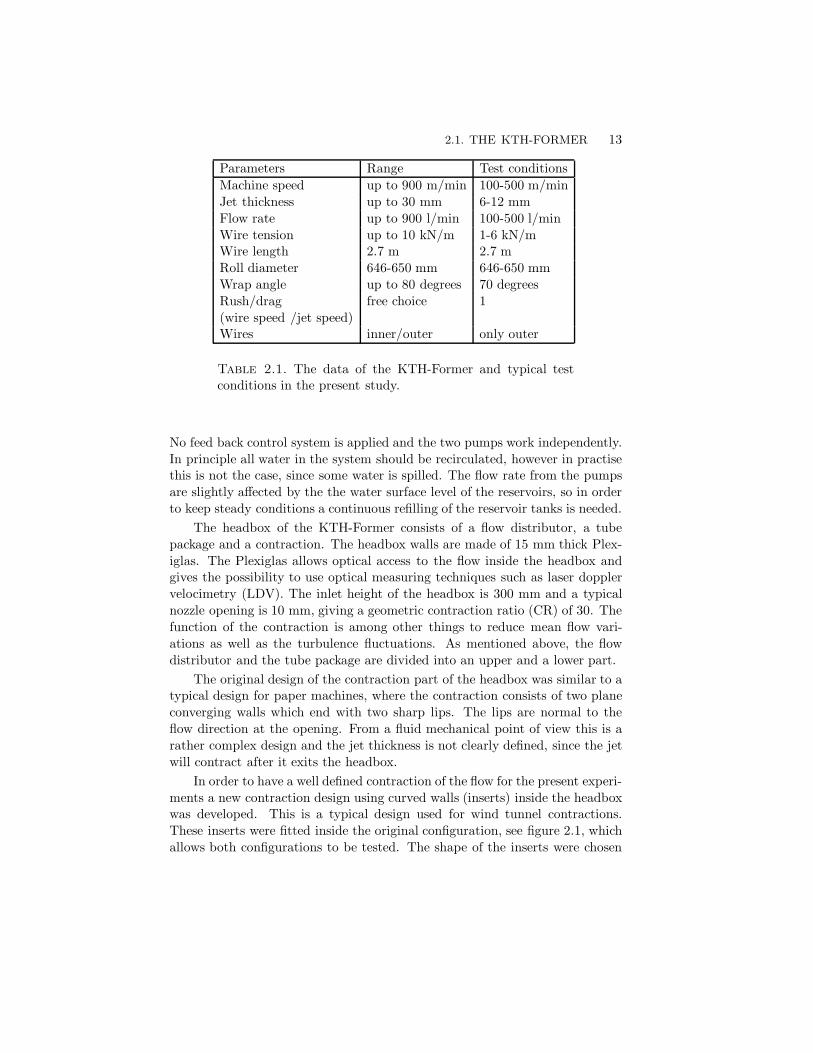
Parameters Range Test conditionsMachine speed up to 900 m/min 100-500 m/minJet thickness up to 30 mm 6-12 mmFlow rate up to 900 l/min 100-500 l/minWire tension up to 10 kN/m 1-6 kN/mWire length 2.7 m 2.7 mRoll diameter 646-650 mm 646-650 mmWrap angle up to 80 degrees 70 degreesRush/drag free choice 1(wire speed /jet speed)Wires inner/outer only outer
Table 2.1. The data of the KTH-Former and typical testconditions in the present study.
No feed back control system is applied and the two pumps work independently.In principle all water in the system should be recirculated, however in practisethis is not the case, since some water is spilled. The flow rate from the pumpsare slightly affected by the the water surface level of the reservoirs, so in orderto keep steady conditions a continuous refilling of the reservoir tanks is needed.
The headbox of the KTH-Former consists of a flow distributor, a tubepackage and a contraction. The headbox walls are made of 15 mm thick Plex-iglas. The Plexiglas allows optical access to the flow inside the headbox andgives the possibility to use optical measuring techniques such as laser dopplervelocimetry (LDV). The inlet height of the headbox is 300 mm and a typicalnozzle opening is 10 mm, giving a geometric contraction ratio (CR) of 30. Thefunction of the contraction is among other things to reduce mean flow vari-ations as well as the turbulence fluctuations. As mentioned above, the flowdistributor and the tube package are divided into an upper and a lower part.
The original design of the contraction part of the headbox was similar to atypical design for paper machines, where the contraction consists of two planeconverging walls which end with two sharp lips. The lips are normal to theflow direction at the opening. From a fluid mechanical point of view this is arather complex design and the jet thickness is not clearly defined, since the jetwill contract after it exits the headbox.
In order to have a well defined contraction of the flow for the present experi-ments a new contraction design using curved walls (inserts) inside the headboxwas developed. This is a typical design used for wind tunnel contractions.These inserts were fitted inside the original configuration, see figure 2.1, whichallows both configurations to be tested. The shape of the inserts were chosen
14 2. EXPERIMENTAL SETUP
to follow a sinh-expression. The design criterion was to avoid separation in thecontraction. In wind tunnel design, the present shape has shown good results,see Lindgren (1999), see also section 2.2 Headbox contraction.
In another study where the present apparatus is used, the behaviour offibre flocs in the dewatering zone of the roll forming is studied and in thatcase the sharp lips will break the flocs that are intentionally introduced beforethe contraction. Also for that study the new design proved to give betterconditions.
In the headbox a centre tube (diameter 8 mm) has been mounted to in-troduce fibre flocs, or a trailing pressure transducer. By this transducer in thejetflow, the pressure could be measured at different streamwise positions bothinside the contraction and in the dewatering zone.
2.1.2. Forming roll and the dewatering zone
The forming roll consists of a Plexiglas cylinder with a nominal diameter of 650mm and a wall thickness of 9 mm. The cylinder is mounted onto a back platemade of aluminum. On the back plate a shaft is mounted which is supportedby two roller bearings and driven by an asynchronous electrical motor (SDM631, 2.7kW). In between the motor and the forming roll a gear drive (BG 247)with a gear ratio of 3.88:1 is installed.
The outer wire roll and the forming roll is speed controlled. The peripheralvelocity of the forming roll will be the same or close to that of the wire. Itis also possible to control the forming roll motor separately, which gives thepossibility to have the roll and/or wire speed to differ from the jet flow speed.
Several Plexiglas cylinders have been made and they can easily be disman-tled from the backplate. The cylinders have been turned and polished to asmooth outer surface with a diameter in the range 646-650 mm. Both endsof the Plexiglas cylinder are covered on the side with a 5 mm thick Plexiglasbarrier, approximately 20 mm larger in radial direction than the roll. Thefunction of the barrier is to prevent leakage and to reduce cross flow in thedewatering zone. The barrier should also guide the wire along the dewateringzone. Inside the forming roll, measurement equipments have been mounted.At the roll centre the slip ring, as well as a support for the local drainage ratemeasuring device are mounted. In the forming roll surface, pre-positioned tapsare mounted for transducer housing. Together with the supporting rolls thiswill form the inner wire track, although in the current study the major part ofthe test was carried out with only an outer wire.
The wire driving cylinder next to the headbox outlet is slightly barrelshaped in order to control the wire position. The position of the upper cylindercan be adjusted in order to vary the wrap angle, whereas the lower cylinder isattached to the wire tension device. In order to trim the wire sideways position,

2.1. THE KTH-FORMER 15
the orientation of this cylinder axis can be adjusted. The headbox itself is alsoadjustable to change the impingement angle, see figure 2.2, which is definedfrom the horisontal line positive in the clockwise direction.
2.1.3. Wire tension
The wire tension varies along the wire path due to friction in the guiding cylin-ders as well as flow drag due to friction between the wire and the surroundingair and water. The highest tension is on the incoming side of the drivingcylinder. However it is estimated that the variation of the wire tension due tofriction effects is small and that to a good approximation the tension could beregarded as constant along the wire path.
Forming roll
Dewatering zone (dwz)
Outer wire
R=0
.325
m
m Pneumatic piston
T1
T2
x
z
Headbox Impingement angle (γ) adjustment
Wrap angle (Φ)(wrap length)adjustment
Wire tension (T)adjustment
Roll rotationalspeed (ωR)
Wire speed (ωw)
Inflow (Q)
α β
M
aa
Figure 2.2. The wire tension set up and adjustment possibilities.
The wire tension was controlled by the lower guiding cylinder which wasmounted on a beam and could move in (mainly) the vertical direction. Themass (M) of the cylinder and its holder was 50 kg, and in order to get an
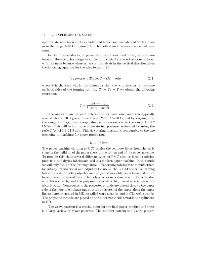
16 2. EXPERIMENTAL SETUP
appropriate wire tension the cylinder had to be counter-balanced with a massm in the range 2–40 kg (figure 2.2). The both counter masses have equal leverarms.
In the original design, a pneumatic piston was used to adjust the wiretension. However, this design was difficult to control and was therefore replacedwith the mass balance adjuster. A static analysis in the vertical direction givesthe following equation for the wire tension (T ),
↑: T1b cosα+ T2b cosβ = (M −m)g (2.1)
where b is the wire width. By assuming that the wire tension is the sameon both sides of the forming roll, i.e. T1 = T2 = T we obtain the followingexpression
T =(M −m)g
b(cosα+ cos β). (2.2)
The angles α and β were determined for each wire, and were typicallyaround 55 and 20 degrees, respectively. With M=50 kg and by varying m inthe range 2–40 kg, the corresponding wire tension was in the range 1.1–3.7kN/m. This will in turn give a dewatering pressure, estimated by using theratio T/R, of 3.3–11.3 kPa. This dewatering pressure is comparable to the oneoccurring in machines for paper production.
2.1.4. Wires
The paper machine clothing (PMC) carries the cellulose fibres from the earlystage in the build up of the paper sheet to the roll up end of the paper machine.To provide this chain several different types of PMC such as forming fabrics,press felts and drying fabrics are used in a modern paper machine. In this studywe will only focus of the forming fabric. The forming fabrics were manufacturedby Albany International and adjusted for use in the KTH-Former. A formingfabric consists of both polyester and polyamid monofilaments (strands) whichhave different material data. The polyester strands show a stiff characteristic,with little stretch, and the polyamid ones show high resistance to wear butabsorb water. Consequently, the polyester strands are placed close to the paperside of the wire to eliminate any rupture or stretch of the paper along the paperline and are orientated in MD, so called warp-strands, and in CD, weft-strands.The polyamid strands are placed on the outer/wear side towards the cylinders,in CD.
The weave pattern is a crucial point for the final paper product and thereis a large variety of weave patterns. The simplest pattern is a 2-shed pattern
2.1. THE KTH-FORMER 17
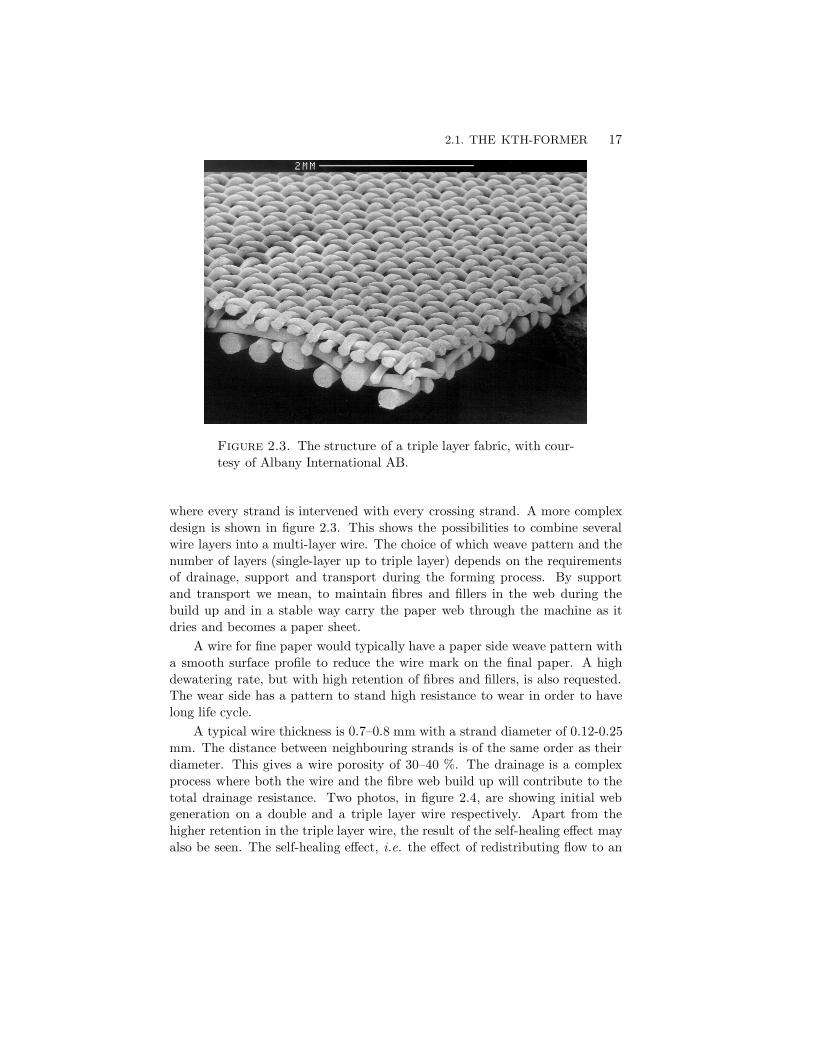
Figure 2.3. The structure of a triple layer fabric, with cour-tesy of Albany International AB.
where every strand is intervened with every crossing strand. A more complexdesign is shown in figure 2.3. This shows the possibilities to combine severalwire layers into a multi-layer wire. The choice of which weave pattern and thenumber of layers (single-layer up to triple layer) depends on the requirementsof drainage, support and transport during the forming process. By supportand transport we mean, to maintain fibres and fillers in the web during thebuild up and in a stable way carry the paper web through the machine as itdries and becomes a paper sheet.
A wire for fine paper would typically have a paper side weave pattern witha smooth surface profile to reduce the wire mark on the final paper. A highdewatering rate, but with high retention of fibres and fillers, is also requested.The wear side has a pattern to stand high resistance to wear in order to havelong life cycle.
A typical wire thickness is 0.7–0.8 mm with a strand diameter of 0.12-0.25mm. The distance between neighbouring strands is of the same order as theirdiameter. This gives a wire porosity of 30–40 %. The drainage is a complexprocess where both the wire and the fibre web build up will contribute to thetotal drainage resistance. Two photos, in figure 2.4, are showing initial webgeneration on a double and a triple layer wire respectively. Apart from thehigher retention in the triple layer wire, the result of the self-healing effect mayalso be seen. The self-healing effect, i.e. the effect of redistributing flow to an

18 2. EXPERIMENTAL SETUP
Figure 2.4. The retention results of the initial web gener-ation on different wires, giving a higher retention for triplelayer wire than double layer wire. left: triple layer wire, right:double layer wire, (courtesy of Albany International AB.)
Figure 2.5. Triple layer wire with CD binder strand. MDvertically in the picture. left: The paper side two-shed, right:The wear side, five shed pattern (courtesy of Albany Interna-tional AB)
area of low local resistance, will result in a more homogeneous paper, see e.g.Norman et al. (1995).
From the fluid mechanics point of view the wire is characterized by itspermeability, which is a measure of the flow resistance through the wire. Forlow velocities, 1–3 m/s, i.e. small Reynolds numbers, the flow through a wirecan be estimated by Darcy’s law

2.1. THE KTH-FORMER 19
q
A=k
µ
∆pd. (2.3)
In the present case this equation relates the flow rate per unit area (q/A) asa function of the pressure difference (∆p) across the wire with a thicknessd. The material parameters entering the expression is the dynamic viscosity(µ) of the fluid and the permeability (k) of the porous material. Hence, thepermeability (k) is a material parameter independent of the fluid in questionand its dimension is L2.
In the present study three different wires were used, one conventional dou-ble layer wire, one partly coated wire (semi-permeable) and one fully coated,non-permeable wire. A polymer primer (polyurethane) was used as coating ofthe wires and it was applied from the wear side of the wire to fill out the poresand to keep the surface structure on the paper side. For the non-permeablewire the coating procedure was repeated until the pores were fully filled. Thecoating had only a small influence on the flexibility of the wire.
Since the major part of the measurements was made without fibres, thesemi-permeable wire was used in order to simulate a fibre web resistance. Thesemi-permeable wire case will initially give rise to a higher drainage resistance(i.e. lower permeability) at impingement and a lower resistance (i.e. higher per-meability) in the later part of the dewatering zone compared to a web built upin a paper machine. However, the average permeability of the semi-permeablewire will in essence simulate the effect of the web build-up on the dewateringprocess.
The determination of the permeability for the various wires was made atAlbany International AB, R&D-department. The determination were madeusing both air and water.
The air test apparatus is an in-house designed test equipment, mainly usedas a production quality check of the wire rather than to be used as a laboratorydetermination of the permeability. It consists of a tube with a diameter of 40mm, and its open end is pressed against a stationary wire. The other end isconnected to a high pressure fan which produces a flow across the wire. Theflow rate (q) is determined by measuring the pressure drop (∆p) across a flangeinside the pipe when keeping an overall pressure drop of approximately 100 Paover the wire. The air permeability can be determined by inserting the flowrate from expression 2.4 into Darcy’s law. Here, α is a specific flange coefficient.
q = απd2
4
√2∆pρ
(2.4)

20 2. EXPERIMENTAL SETUP
0.05
0.1
0.15
0.2
0.25
0.3
0.35
(Q/A
), [m
/s] a
ir te
st
Measurement
Figure 2.6. Air test data for the semi-permeable wire casefor different measurements, mean value 0.17 with a standarddeviation of 0.049 m/s.
In the water test procedure a commercial apparatus the L&W ScanproFeltperm was used. The principle is similar to the air test but the wire mustbe moving when performing the measurements. The special wire nozzle, (1 mmin diameter) was placed towards the wire and the flow rate of the jet passingthrough the wire was measured for a pressure drop across the wire of 300 kPa.This method is often used as a quick test on the status of the wire in a papermachine and can be carried out during running condition. The test proceduregives a value of the MD variation but could also give a estimation of the CDvariation of the wire permeability by scanning over the spanwise direction ofthe wire.
In the present study, both methods have been used to determine the per-meability for the semi-permeable wire and the conventional wire. The twomethods should give the same value of the permeability. As can be seen in ta-ble 2.2 the permeability for the semi-permeable wire was reduced considerablycompared to the conventional one. However, the permeability showed someMD variations, figure 2.6, due to the difficulty in applying the coating evenlyalong its length. But the variation will not in general influence the desiredrequirement of having a lower permeability.
2.2. Headbox contraction
The headbox contraction, as described earlier, differs from a conventional head-box used in paper machines (see figure 2.7). The shape was described with ananalytical expression, which was adjusted to give a zero slope at the entrance

2.2. HEADBOX CONTRACTION 21
Wire air test (standard) water test Est. permeability kq/A [m/s] q/A [m/s] [m2]
General datadouble layer wire 1.4–1.9 - 2.8–3.8·10−10
triple layer wire 1.3–1.8 - 2.6–3.6·10−10
specific test wiressemi-permeable wire 0.17 8 [0.34, 0.27]·10−10
double layer wire 61 2·10−10
Non-permeable - - -
Table 2.2. Permeability data for different wires carried outwith the two methods.
Figure 2.7. The headbox contraction with its inserts, partlyfilled with water.
and exit. The actual shape of the insert was described by the following expres-sion and proved to fulfill the design criterion of avoiding separation along thecontraction. This shape has been used in wind tunnel designs.
y =
0 if x ≤ 0A sinh(Bx) − Bx 0 < x ≤ 0.71− C sinh(Dx) −Dx 0.7 < x ≤ 11 if x > 1
where the constants (A-D) were set to [0.205819, 3.52918, 0.08819, 8.23523].
22 2. EXPERIMENTAL SETUP
0 50 100 150 200 250 300 350 400 4500
0.5
1
1.5
2
2.5
3
3.5
4
4.5
5
5.5
velo
city
[m/s
]
Position in contraction [mm]
LDV-datatheoretical data
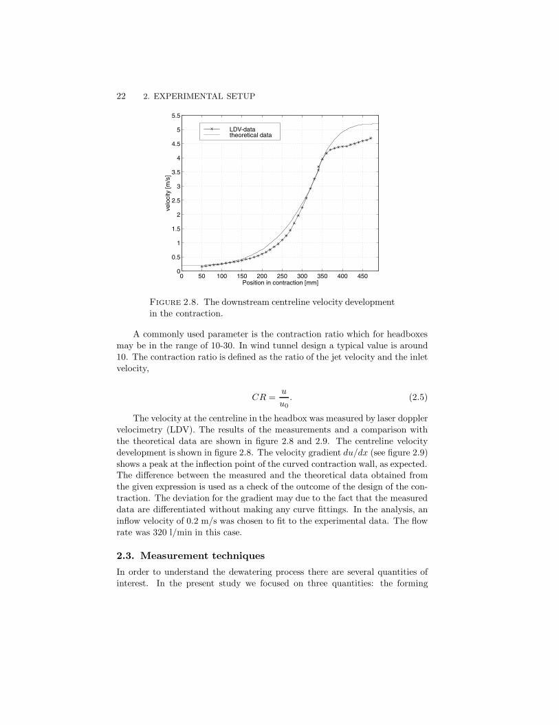
Figure 2.8. The downstream centreline velocity developmentin the contraction.
A commonly used parameter is the contraction ratio which for headboxesmay be in the range of 10-30. In wind tunnel design a typical value is around10. The contraction ratio is defined as the ratio of the jet velocity and the inletvelocity,
CR =u
u0. (2.5)
The velocity at the centreline in the headbox was measured by laser dopplervelocimetry (LDV). The results of the measurements and a comparison withthe theoretical data are shown in figure 2.8 and 2.9. The centreline velocitydevelopment is shown in figure 2.8. The velocity gradient du/dx (see figure 2.9)shows a peak at the inflection point of the curved contraction wall, as expected.The difference between the measured and the theoretical data obtained fromthe given expression is used as a check of the outcome of the design of the con-traction. The deviation for the gradient may due to the fact that the measureddata are differentiated without making any curve fittings. In the analysis, aninflow velocity of 0.2 m/s was chosen to fit to the experimental data. The flowrate was 320 l/min in this case.
2.3. Measurement techniques
In order to understand the dewatering process there are several quantities ofinterest. In the present study we focused on three quantities: the forming

2.3. MEASUREMENT TECHNIQUES 23
0 50 100 150 200 250 300 350 400 4500
0.005
0.01
0.015
0.02
0.025
0.03
0.035
0.04
du/d
x
Position in contraction [mm]
LDV-datatheoretical data
0 5 10 15 20 25 300
0.005
0.01
0.015
0.02
0.025
0.03
0.035
0.04
du/d
x
Contraction
LDV-datatheoretical data
Figure 2.9. left: Velocity gradient vs. position, right: Ve-locity gradient vs. contraction ratio.
roll surface pressure, the position of the wire relative to the forming roll andthe dewatering/ drainage rate. These quantities were measured for variouscombinations of parameter settings, such as the wire tension, the inflow rateand the wire type. Other settings are the impingement angle, the wrap angle,the ratio jet speed to wire speed (rush/ drag), the water jet thickness and alsothe fibre concentration. All these were mainly kept constant in the presentstudy, see chapter 3.
The measurements of the pressure and the wire position were made in therotating system by having the devices mounted inside the forming roll. Thisincluded transducers, amplifiers and connectors. The pressure signal was thenamplified before being transferred over the slip ring device whereas the wireposition signal could pass without any signal conditioning. A high qualityslip-ring assembly with 8 silver plated rings was used for the power supplyand for the signal transfer to the acquisition system. In order to start themeasurements a magneto-resistive sensor (KMZ10) was used. The sensor wasfixed at the support stand and a magnet was glued on the forming roll. Thistriggering sensor gave a consistent reference starting signal of each data setwhen the magnet mounted on the roll passed the sensor. This will be used asthe reference start point in all results. A typical duration of the passage ofthe roll fixed transducer through the dewatering zone is of the order of 0.1 s.Consequently, the choice of transducers is limited to those with a short responsetime.
The dewatering collector (saveall) was movable around the forming rollcentre. By choosing this set up, the dewatering zone could be covered bymoving and adjusting the saveall to each position along the zone, see figure2.11.

24 2. EXPERIMENTAL SETUP
Triggering transducer
Jet inflow
Pressure transducer
Position transducer
Save all
x
y
Forming roll
Figure 2.10. An illustration of the measurement set up. Thetriggering point will be used as the reference point in all results.Here the wire position and pressure transducers are placed inopposite positions, but they could also be placed next to eachother.
For each setting, several data sets were measured to secure that the resultswere reproducible. This includes both several readings as the forming rollrotates and also in repeated measurements for the same settings. There wasa certain time until steady state of the total flow system was obtained. Somewater is not recirculated but is wasted, so the reservoirs need to be continuouslyrefilled in order to keep the flow conditions constant. Therefore, there weresome problems keeping the working conditions constant during a measurementsession, but after some practice reasonably stable conditions were achieved.
2.3.1. Pressure measurements
In order to carry out measurements of the pressure on the rotating cylinder thetransducer has to fulfill several requirements. For successful operation it shouldbe robust, have a waterproof membrane and water resistant housing. It shouldalso be possible to mount flush with the surface, have sufficiently small size,have a high dynamic response and high sensitivity and also be able to measure

2.3. MEASUREMENT TECHNIQUES 25
Figure 2.11. The arrangement with the saveall in the dewa-tering zone
negative pressures. Some of these requirements are however contradictory, e.g.robustness and sensitivity.
Most of the pressure measurements were carried out with surface mountedpressure transducers but some measurements were also carried out with a freetrailing transducer in the jet. In the forming roll mounted case, the membranehead was adjusted to be flush with the forming roll surface to measure the dy-namic changes in the pressure as it passed through the dewatering zone. Thetime within the zone was less than 0.1 s. The reason to place the membraneclose to the surface was to reduce the influences of possible air bubble or cap-illary effects that could disturb the measurement. To avoid any by-pass waterleakage into the forming roll, a gasket supported by silicone, was used.
A small, flush mounted transducer, sensitive to low pressure tends to bevery sensitive to any shock, particularly in the membrane plane. A high tan-gential shear could destroy the transducer. A particle hitting the membranecould also damage the sensor. The fact that the transducer should work inwater limited the number of possible transducers. The small transducer headwas required in order to get the local pressure and also not to alter the shape ofthe cylindrically curved roll surface. This finally resulted in that two differenttypes of transducers were used, one piezoresistive (Endevco 8507C-2) and onestrain-gauge transducer (Entran EPX-N01). In both cases, the long deliverytime was a limiting factor.
The advantages of the piezoresistive transducer are high response frequency(125 kHz), signal symmetry around the reference pressure (± 14 kPa), but itis less robust and only partly waterproof. To extend the life time in water a

26 2. EXPERIMENTAL SETUP
coating of silicone or parylen (in this study parylen was used) is often applied.The main disadvantage of that particular transducer was its limited robustness.In the case of the strain-gauge transducer, the membrane of aluminumwas morerobust and waterproof but the transducer showed a less dynamic response (50kHz). It was slightly larger (diameter 3 mm), with a measuring range up to70 kPa, but it could only withstand negative pressures. However, negativepressures influenced the return to zero of the membrane and this was moreapparent when returning from low negative than from high negative pressure.The advantage of waterproofness and robustness for many cycles, and also itsavailability led to the use of the strain-gauge transducer as the default one.
0.05 0.1 0.15 0.2 0.25 0.3
-3
-2.5
-2
-1.5
-1
-0.5
0
0.5
p/p_
max
Normalised wrap angle
Entran, p_max=8.8 kPaEndevco, p_max=4.4 kPa
Figure 2.12. Comparison of the two different transducertypes mounted flush with the forming roll surface for a non-permeable wire case. The cases are different but the pressuresare normalised with the maximum pressure.
A comparison between the two types is shown in figure 2.12. The pressurehave been normalised with its maximum for each case. They show the samepressure characteristics, but not in the early stage, which is due to a set up witha different impingement angle. The ratio of the pressure peaks are in fairly goodagreement even for the very low suction peak at the end of the dewatering zone.The slow recovery to zero of the Entran transducer is partly seen in figure 2.12and it became a growing problem during the test. The difference from zero at0.25 will slowly recover to zero due to the dynamic response time for negativepressure when no outer pressure was applied. So, consequently this indicatedpressure does not corresponds to any physical pressure but is rather an effectof the transducer type.

2.3. MEASUREMENT TECHNIQUES 27
Figure 2.13 shows five consecutive measurements with the Entran-transducer.All measurements start at zero pressure so the transducer has recovered thezero-level before the measurement starts. As can be seen there is a slight vari-ation between the different runs. In the figure the variation, expressed as thestandard deviation (std), is presented as well (for a total of ten measurementseries). The standard deviation shows a peak at the exit of the dewatering zoneas expected since also small differences in time will give large variations, dueto the large amplitude signal. The variations observed in this figure are typicalfor the measurements performed.
0.1 0.15 0.2 0.25 0.3
0
-30
-20
-10
0
10
Pre
ssur
e [k
Pa]
Normalised wrap angle
pressurestd
Figure 2.13. Consecutive measurements each revolution andits standard deviation, Entran-transducer, non-permeable wirecase.
An alternative way, as compared to the roll-mounted pressure transducer,is to use a free trailing transducer in the flow. The position of the transducer inthe dewatering zone has to be recorded and by this method the variation at acertain position in the zone could be measured for a longer time sequence thanby the roll fixed transducer method. For this we used a micro transducer fromSAMBA Sensors AB with a Samba 3000 Controller. This technique is usedfibre-optics and is based on the Fabry-Perot principle. The sensor element issmall, with a diameter of approximately 0.42 mm and has a supporting opticalfibre cable with a diameter of 0.2 mm. The fibre has high tensile strength butthe surface is sensitive to wear. The fibre and the sensor head were thereforecovered with a silicone tubing of 1.2 mm in diameter. In the experimentalset up the Samba sensor could either be introduced in the mid section of theheadbox or just before the impingement zone directly into the water jet at thecentreline. The positioning was simply made with a ruler to determine the

28 2. EXPERIMENTAL SETUP
MD position in the dewatering zone. The MD position was rather consistentapart from the end part of the dewatering zone, where it was impossible toobserve the head and even harder to control the spanwise position. The radialposition was not controlled but the observation indicated that the sensor headwas closer to the wire than to the forming roll, see in chapter 4 Results.
The Samba sensor is an absolute pressure transducer with a more or lessfixed lower limit of -5 kPa, the upper range is set after request, in this caseit was set to 25 kPa. The response frequency was 500 Hz. This was enoughsince for these measurements the probe is stationary. In the present study theSamba sensor was only used as a complementary check of the roll mountedtransducers, but the techniques is very interesting since the method could beapplied also in a real paper machine.
In conclusion it was found that it was difficult to find a transducer thatfulfilled all requirements to give consistent and repeatable measurements. Thespecific data of the transducers which were used are presented in table 2.3. TheSamba sensor is an absolute transducer whereas the other two that are venteddifferential transducers. This proved to be a problem after long time usage,when a zero drift was noticed due to moisture in the vented ones.
Transducer type model pressure responseEndevco piezoresistive 8507C-2 ± 14 kPa 70 kHzEntran strain gauge EPX-N01-0.7B up to 70 kPa 50 kHzSamba fibre-optic Samba-250 -5 up to 25 kPa 500 Hz
absolute
Table 2.3. Pressure transducer
The transducers (Entran and Endevco) were calibrated before and afterthe experiments with a DRUCK DP610 Calibrator. This calibrator has anaccuracy of 0.025% of FS (Full Scale 1 bar). They were linear as expected. Inorder to reduce noise in the signal, the pressure signal was amplified before itwas fed to the slip-ring assembly. An in-house built amplifier and an Entranamplifier (IAM Amplifier 1505-50) with 250 and 1000 times amplification wasused together with a RDP-S7DC with variable amplification.
In the forming roll, the pressure transducers could be mounted at threedifferent spanwise positions: at the centreline and two position on each side,20 mm and 40 mm respectively from the centreline. This was carried out tostudy the possible spanwise differences, and in a region of 40 mm around themidsection no such differences were observed, figure 2.14. Thus the side barriersare efficient to reduce CD flow. The pressure transducer was also placed nextto the wire position pin, see figure 2.15, to examine any possible influences, but

2.3. MEASUREMENT TECHNIQUES 29
0.04 0.06 0.08 0.1 0.12 0.14 0.16 0.18 0.2 0.22-30
-25
-20
-15
-10
-5
0
5
10
Pre
ssur
e [k
Pa]
Norm. wrap angle
Transducer 1Transducer 2
Figure 2.14. Comparison of different spanwise positions ofthe Entran-transducer in the forming roll, transducer 1 referto the one at centre, transducer 2 is mounted 20 mm off centreline, non-permeable wire case.
Figure 2.15. The close up of the transducers, the position pinin the rear left with the end plate and the pressure transducernext to it
marginal differences were recorded. Finally, pressure measurement were carriedout simultaneously with the drainage measurements to observe influences ofthe collector (saveall), but if it was gently positioned to the wire, no significantinfluence was observed.

30 2. EXPERIMENTAL SETUP
2.3.2. Wire position measurements
In the present study we used a mechanical method to measure the wire positionin the dewatering zone. A resistive linear potentiometer (Sakae S8FLP-10A)with a spring loaded pin was mounted on the forming roll. When the wireenters the dewatering zone the pin mechanically gets into contact with thewire. The spring force on the pin of 10 N keeps the pin in contact with thewire. In order to reduce the influence of the pin pushing locally on the wire acircular plate with a diameter of 5 mm was mounted on the top of the pin, seephoto 2.15. The thickness of the plate was 1 mm.
0.06 0.08 0.1 0.12 0.14 0.16 0.18 0.2 0.220
2
4
6
8
10
12
14
16
Wire
pos
ition
[mm
]
Norm. wrap angle
positionstd
Figure 2.16. Consecutive measurements for each revolutionand its standard deviation, non-permeable wire case.
A typical set of five different position measurements is shown in figure2.16. As can be seen there is a slight variation between the different cases. Thecorresponding standard deviation is also seen in the figure. The radial positionof the pin has to be adjusted and calibrated before and after each test. Thefull range of the transducer is 13 mm. For one of the measurements in this casethe position transducer was fully immersed. This is seen at the very last of thesignal in figure 2.16 (at 0.21 wrap angle units) as a plateau at 5 mm. However,in order to avoid this, in a later modification of the transducer the measuringrange was extended by using a lever arrangement.
In order to evaluate the wire position technique, measurements were per-formed on the roll-wire set up without any water. For this case the trajectoryof the position pin in the entry and the exit part could be derived analytically.The geometry and the appropriate angles are seen in figure 2.17. The horisontallines indicate the tangential approach of the wire to the roll with and without

2.3. MEASUREMENT TECHNIQUES 31
water. In the case of no water the distance (g) between roll and wire will followthe expression,
g(θ) = R(1
cos θ− 1) (2.6)
where R is roll radius and θ is the angle defined in figure 2.17. In the resultsection a comparison between measured data and this expression will be shown.
ds
∆r=gR
R
α
∆r
θψ=θ−α
β γν∆h
Figure 2.17. Schematic view of when the wire enters theroll, the solid line with radius R is the roll and the dash linecorresponds to the circumference of the top of the untouchedwire position pin.
2.3.3. Local dewatering measurements
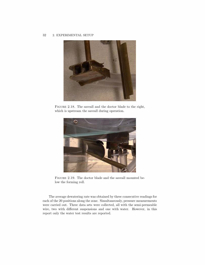
The dewatering/drainage rate was measured by a 15 × 10 mm double boxcollector, fixed at the centre bearing of the forming roll and along the formingroll periphery, on the dewatering side of the wire. The collector, also calleda ”saveall” was designed with a spring adjuster instead of being fixed in theradial position, in order to avoid influences on the wire. It was also flexible inboth the cross direction and the tangential angle to resolve data in the foremostpart and in the end part of the dewatering zone. The elongation of the box wassmall compared to the forming roll curvature. The expelled water was collectedlocally during a time (15–20 s) for each position from the both collector boxes.A shift downstream could be carried out in desired steps and an overlap of onebox was used in each step. In order not to collect the water along the wire adoctor blade was used. This was placed upstream of the saveall, see in figure2.19 to remove the incoming water.
32 2. EXPERIMENTAL SETUP
Figure 2.18. The saveall and the doctor blade to the right,which is upstream the saveall during operation.
Figure 2.19. The doctor blade and the saveall mounted be-low the forming roll.
The average dewatering rate was obtained by three consecutive readings foreach of the 20 positions along the zone. Simultaneously, pressure measurementswere carried out. Three data sets were collected, all with the semi-permeablewire, two with different suspensions and one with water. However, in thisreport only the water test results are reported.
2.4. DATA ACQUISITION 33
2.4. Data acquisition
For data acquisition, a Macintosh Quadra 950 was available with a 16 bit and8 channel A/D-board. The power supply to the transducers as well as thesignals had to pass over the slip rings in the forming roll. A Labview softwarewas serving as the data reading program. Data were acquired for typically5–15 passages, while keeping the test conditions constant in order to check thereproducibility. The acquisition rate for the pressure and the wire positionmeasurements were between 1000-20000 Hz and for the Samba sensor it was500 Hz. This resulted in approximately 2000-3000 measurement points withinthe dewatering zone for the pressure and the wire position.

34 2. EXPERIMENTAL SETUP

CHAPTER 3
Theoretical considerations of roll forming
Roll forming is a complex physical process and the dewatering pressure is influ-enced by many different parameters. The most simple model of the dewateringpressure can be expressed as
p =T
R
where p is the pressure between the wires and T and R are the wire tensionand roll radius respectively. The results of the present work clearly show thatthe pressure is far from described by this simple relation.
3.1. Dimensional analysis
In order to determine the relevant non-dimensional groups of variables in theroll forming problem a dimensional analysis of the problem is useful. In thepresent problem all variables can be expressed in terms of three reference mag-nitudes, namely mass [M], length [L] and time [T].
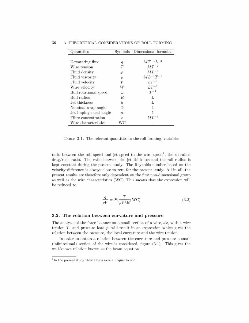
In the roll forming problem the interesting process quantity is the dewa-tering (q) which will be dependent on a number of different types of variables.These are referred to as geometrical (roll radius (R), nominal wrap angle (Φ),jet thickness (h) and jet impingement angle (α)), fluid specifics (viscosity (µ),density (ρ) and fibre concentration (c)), process specific (jet (V ) and wire(W ) velocity, roll rotational speed (ω) and wire tension (T )) as well as thewire characteristics (WC). The relevant quantities are presented in table 3.1together with their dimensional formulae.
The dimensional analysis gives the following non-dimensional groups,
q
ρV= F(
T
ρV 2R,ωR
V,W
V,h
R,ρ|V −W |h
µ;α,Φ, c,WC) (3.1)
where α and Φ were fixed during the present study and therefore can be viewedas parameters, no fibres were present (c = 0), and three distinct differently wireswere used (WC).
The normalized dewatering flux is determined by the four non-dimensionalgroups in equation (3.1), the nominal pressure to the jet dynamic pressure, the
35
36 3. THEORETICAL CONSIDERATIONS OF ROLL FORMING
Quantities Symbols Dimensional formulae
Dewatering flux q MT−1L−2
Wire tension T MT−2
Fluid density ρ ML−3
Fluid viscosity µ ML−1T−1
Fluid velocity V LT−1
Wire velocity W LT−1
Roll rotational speed ω T−1
Roll radius R LJet thickness h LNominal wrap angle Φ 1Jet impingement angle α 1Fibre concentration c ML−3
Wire characteristics WC -
Table 3.1. The relevant quantities in the roll forming, variables
ratio between the roll speed and jet speed to the wire speed1 , the so calleddrag/rush ratio. The ratio between the jet thickness and the roll radius iskept constant during the present study. The Reynolds number based on thevelocity difference is always close to zero for the present study. All in all, thepresent results are therefore only dependent on the first non-dimensional groupas well as the wire characteristics (WC). This means that the expression willbe reduced to,
q
ρV= F(
T
ρV 2R;WC) (3.2)
3.2. The relation between curvature and pressure
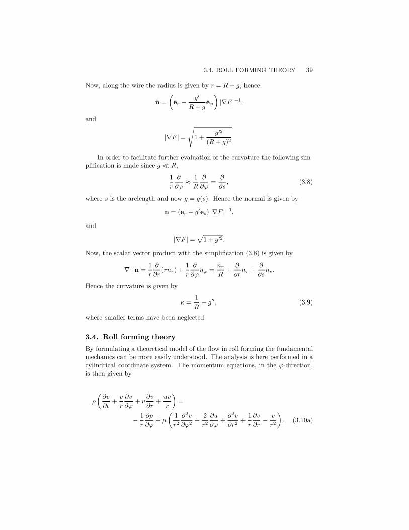
The analysis of the force balance on a small section of a wire, dx, with a wiretension T , and pressure load p, will result in an expression which gives therelation between the pressure, the local curvature and the wire tension.
In order to obtain a relation between the curvature and pressure a small(infinitesimal) section of the wire is considered, figure (3.1). This gives thewell-known relation known as the beam equation
1In the present study these ratios were all equal to one.

3.3. WIRE CURVATURE IN CYLINDRICAL COORDINATES 37
p(x) dx
SaTa
νa Ma
Tb
νb
Sb
Mb
Figure 3.1. The force balance on a wire section ∆x
Td2y
dx2−EI
d4y
dx4− p(x) = 0 (3.3)
where EI is the bending stiffness. Now, with the assumption that the wirebending stiffness can be neglected, the relation between wire curvature andpressure becomes
p(x) = Td2y
dx2(3.4)
whered2y
dx2can be viewed as the linearized curvature term.
3.3. Wire curvature in cylindrical coordinates
The geometry of the problem makes it an advantage to perform the analysis incylindrical coordinates. The wire position in the cylindrical coordinate system,is given by the following equation
F (r, ϕ) = 0 (3.5)
where
F (r, ϕ) = r − R− g(ϕ).
In this equation R is the cylinder radius, g(ϕ) the distance between wireand roll surface (in the r-direction) and r and ϕ are the radial and azimuthalcoordinates respectively. Hence the equation describes the wire as a curve inthe r − ϕ plane. The general definition of the radius of curvature ( is

38 3. THEORETICAL CONSIDERATIONS OF ROLL FORMING
g(φ)
RR
φ
φ
Wire
Figure 3.2. The definition of distance r to the wire, r = R+g,in the cylindrical coordinate system.
( =1κ
where κ is the curvature defined as
κ = ∇ · n. (3.6)
Here
n = nrer + nϕeϕ
is the normal to the wire, which is given by
n =∇F|∇F |.
Hence κ, eq. (3.6), can be written as
κ = ∇ · ∇F|∇F |. (3.7)
This can now be applied to the equation describing the path of the wire,eq. (3.5). The nabla operator in cylindrical coordinates,
∇f(r, ϕ) = ∂f
∂rer +
1r
∂f
∂ϕeϕ,
can now be applied to (3.5), which gives
n =(er −
g′
reϕ
)|∇F |−1.
In this expression
|∇F | =√1 +
g′2
r2.
3.4. ROLL FORMING THEORY 39
Now, along the wire the radius is given by r = R+ g, hence
n =(er −
g′
R+ geϕ
)|∇F |−1.
and
|∇F |=√
1 +g′2
(R+ g)2.
In order to facilitate further evaluation of the curvature the following sim-plification is made since g � R,
1r
∂
∂ϕ≈ 1R
∂
∂ϕ=
∂
∂s, (3.8)
where s is the arclength and now g = g(s). Hence the normal is given by
n = (er − g′es) |∇F |−1.
and
|∇F | =√1 + g′2.
Now, the scalar vector product with the simplification (3.8) is given by
∇ · n =1r
∂
∂r(rnr) +
1r
∂
∂ϕnϕ =
nr
R+
∂
∂rnr +
∂
∂sns.
Hence the curvature is given by
κ =1R
− g′′, (3.9)
where smaller terms have been neglected.
3.4. Roll forming theory
By formulating a theoretical model of the flow in roll forming the fundamentalmechanics can be more easily understood. The analysis is here performed in acylindrical coordinate system. The momentum equations, in the ϕ-direction,is then given by
ρ
(∂v
∂t+v
r
∂v
∂ϕ+ u
∂v
∂r+uv
r
)=
− 1r
∂p
∂ϕ+ µ
(1r2
∂2v
∂ϕ2+
2r2∂u
∂ϕ+∂2v
∂r2+
1r
∂v
∂r− v
r2
), (3.10a)
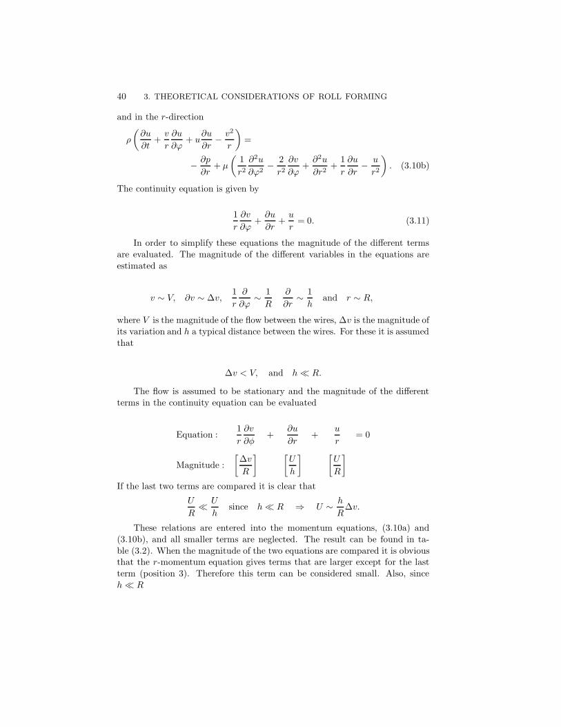
40 3. THEORETICAL CONSIDERATIONS OF ROLL FORMING
and in the r-direction
ρ
(∂u
∂t+v
r
∂u
∂ϕ+ u
∂u
∂r− v2
r
)=
− ∂p
∂r+ µ
(1r2∂2u
∂ϕ2− 2r2∂v
∂ϕ+∂2u
∂r2+
1r
∂u
∂r− u
r2
). (3.10b)
The continuity equation is given by
1r
∂v
∂ϕ+∂u
∂r+u
r= 0. (3.11)
In order to simplify these equations the magnitude of the different termsare evaluated. The magnitude of the different variables in the equations areestimated as
v ∼ V, ∂v ∼ ∆v,1r
∂
∂ϕ∼ 1R
∂
∂r∼ 1h
and r ∼ R,
where V is the magnitude of the flow between the wires, ∆v is the magnitude ofits variation and h a typical distance between the wires. For these it is assumedthat
∆v < V, and h � R.
The flow is assumed to be stationary and the magnitude of the differentterms in the continuity equation can be evaluated
Equation :1r
∂v
∂φ+
∂u
∂r+
u
r= 0
Magnitude :[∆vR
] [U
h
] [U
R
]If the last two terms are compared it is clear that
U
R� U
hsince h� R ⇒ U ∼ h
R∆v.
These relations are entered into the momentum equations, (3.10a) and(3.10b), and all smaller terms are neglected. The result can be found in ta-ble (3.2). When the magnitude of the two equations are compared it is obviousthat the r-momentum equation gives terms that are larger except for the lastterm (position 3). Therefore this term can be considered small. Also, sinceh � R
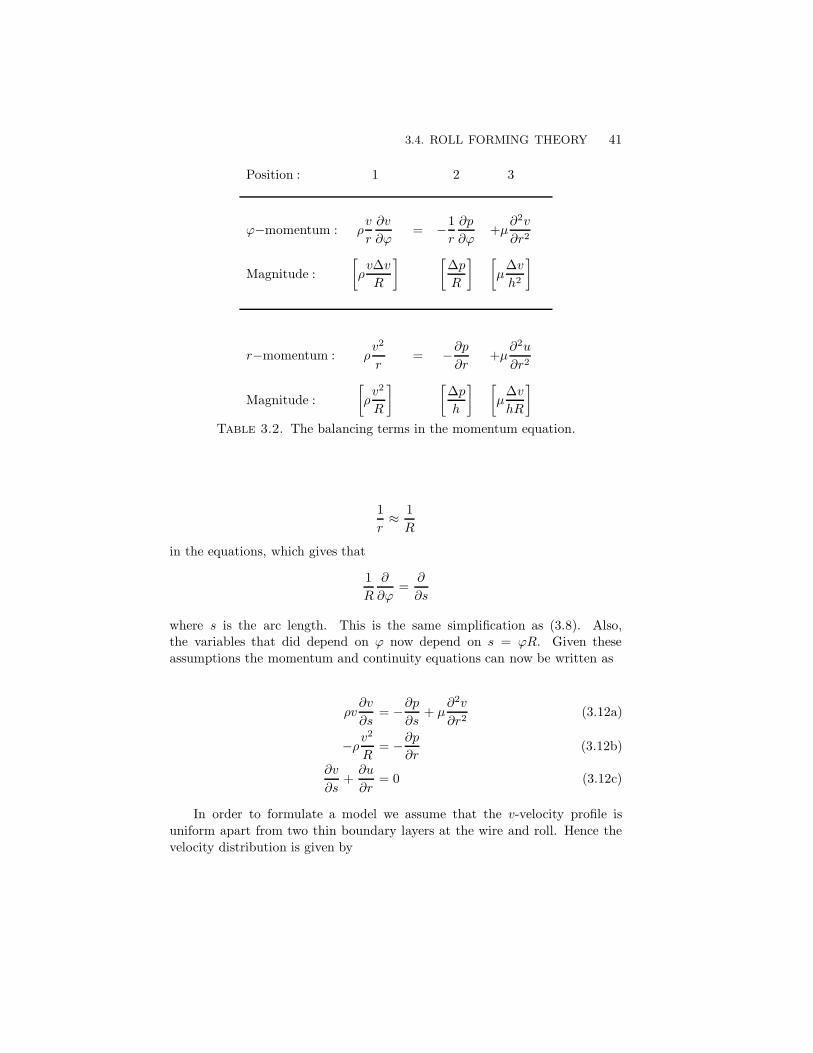
3.4. ROLL FORMING THEORY 41
Position : 1 2 3
ϕ−momentum : ρv
r
∂v
∂ϕ= −1
r
∂p
∂ϕ+µ
∂2v
∂r2
Magnitude :[ρv∆vR
] [∆pR
] [µ∆vh2
]
r−momentum : ρv2
r= −∂p
∂r+µ
∂2u
∂r2
Magnitude :[ρv2
R
] [∆ph
] [µ∆vhR
]Table 3.2. The balancing terms in the momentum equation.
1r≈ 1R
in the equations, which gives that
1R
∂
∂ϕ=
∂
∂s
where s is the arc length. This is the same simplification as (3.8). Also,the variables that did depend on ϕ now depend on s = ϕR. Given theseassumptions the momentum and continuity equations can now be written as
ρv∂v
∂s= −∂p
∂s+ µ
∂2v
∂r2(3.12a)
−ρv2
R= −∂p
∂r(3.12b)
∂v
∂s+∂u
∂r= 0 (3.12c)
In order to formulate a model we assume that the v-velocity profile isuniform apart from two thin boundary layers at the wire and roll. Hence thevelocity distribution is given by

42 3. THEORETICAL CONSIDERATIONS OF ROLL FORMING
v(r) =
V (s)f(s, r −R) R ≤ r < R+ δ
V (s) R+ δ ≤ r ≤ R+ g − δ
V (s)f(s, R + g − r) R+ g − δ < r ≤ R+ g
where δ is the typical boundary layer thickness and f(s, r) is the boundarylayer velocity distribution. The pressure at the roll side of the wire is assumedto be given by the curvature and atmospheric pressure
pw(s) = Tκ(s) + pa, (3.13)
where pw is the pressure at the wire, pa the atmospheric pressure, T the wiretension and κ the wire curvature, which is given by (3.9).
In order to solve the system of equations (3.12) the r-momentum equation,(3.12b), is integrated as
ρ
∫ R+g
r
v2
Rdr =
∫ R+g
r
∂p
∂rdr,
which gives
p(s, r) = pw(s) − ρ
∫ R+g
r
v2
Rdr.
This is inserted into the ϕ-momentum equation, (3.12a),
ρ
2∂v2
∂s= −∂pw
∂s+
ρ
R
∂
∂s
∫ R+g
r
v2 dr + µ∂2v
∂r2. (3.14)
Now, equation (3.14) is integrated from the roll to the wire,
ρ
2
∫ R+g
R
∂v2
∂sdr =
−∫ R+g
R
∂pw
∂sdr +
ρ
R
∫ R+g
R
∂
∂s
(∫ R+g
r
v2 dr
)dr + µ
∫ R+g
r
∂2v
∂r2dr. (3.15)
The first term on the right hand side, i.e. the “wire” pressure term, is only a
function of s. Hence, ∫ R+g
R
∂pw
∂sdr =
dpw
dsg = p′wg
The last integration term is given by

3.4. ROLL FORMING THEORY 43
µ
∫ R+g
R
∂2v
∂r2dr = µ
[∂v∂r
]R+g
R= −2µ
∂v
∂rR
,
where the gradients at the roll and wire are assumed to have the same magni-tude but opposite signs. For the other three terms in eq. (3.15) the integrationis now considered to be performed in three steps. This is exemplified with thefirst term,
ρ
2
∫ R+g
R
∂v2
∂sdr =
ρ
2
∫ R+δ
R
∂v2
∂sdr +
ρ
2
∫ R+g−δ
R+δ
∂v2
∂sdr +
ρ
2
∫ R+g
R+g−δ
∂v2
∂sdr
The boundary layer thicknesses at the wire and roll are assumed to be smallcompared to the distance between the wire and roll. All three integration termshave the same sign and the middle term is assumed to be dominant hence thefollowing simplification is made
ρ
2
∫ R+g
R
∂v2
∂sdr ≈ ρ
2
∫ R+g−δ
R+δ
∂v2
∂s≈ ρ
2dV 2
dsg =
ρ
2(V 2)′g.
The same simplification is made on the last two remaining integration termsin eq. (3.15) and the result is
ρ
2(V 2)′g = −p′wg +
ρ
RV 2g′g +
ρ
2R(V 2)′g2 − 2µ
∂v
∂rR
. (3.16)
Since there is no dewatering the velocity V is given by
V =Q
g, (3.17)
where Q is the volume flow/width between the roll and wire. With this relationthe second and third term on the right hand side of equation (3.16) can beevaluated as
ρ
RV 2g′g +
ρ
2R(V 2)′g2 = +
ρ
2RV 2(g2)′ +
ρ
2R(V 2)′g2 =
ρ
2R(V 2g2)′ =
ρ
2R(Q2)′ = 0,
since Q is a constant. Thus, with the relation for the wire pressure, (3.13), themodel equation is as follows,
44 3. THEORETICAL CONSIDERATIONS OF ROLL FORMING
ρ
2
(Q2
g2
)′g = −Tκ′g − 2µ
∂v
∂rR
.
If the effect of shear is neglected and the expression for the curvature, (3.9), isused this can be written as
g′′′g3 +ρQ2
Tg′ = 0 (3.18)
3.4.1. Linearized solution
Given the equation (3.18) a disturbance is introduced as g = g0 + g whereg � g0. The disturbance satisfies the equation and represents a constantdistance between the wire and roll. After linearization this can be written as
g′′′ +ρQ2
Tg30
g′ = 0
From this equation we can define a non-dimensional Weber number, defined as
We =ρQ2
Tg0(3.19)
giving the final equation as
g′′′ +We
g20
g′ = 0 (3.20)
The solution is assumed to have the form g = geλs, which is inserted intothe equation. This gives the following expression
λ(λ2 +We
g20
)g = 0, (3.21)
which has the following solutions
λ =
0
±i√We
g20
(3.22)
This either gives a solution with a constant distance between the roll and wireor a standing wave solution with a given wavenumber.

CHAPTER 4
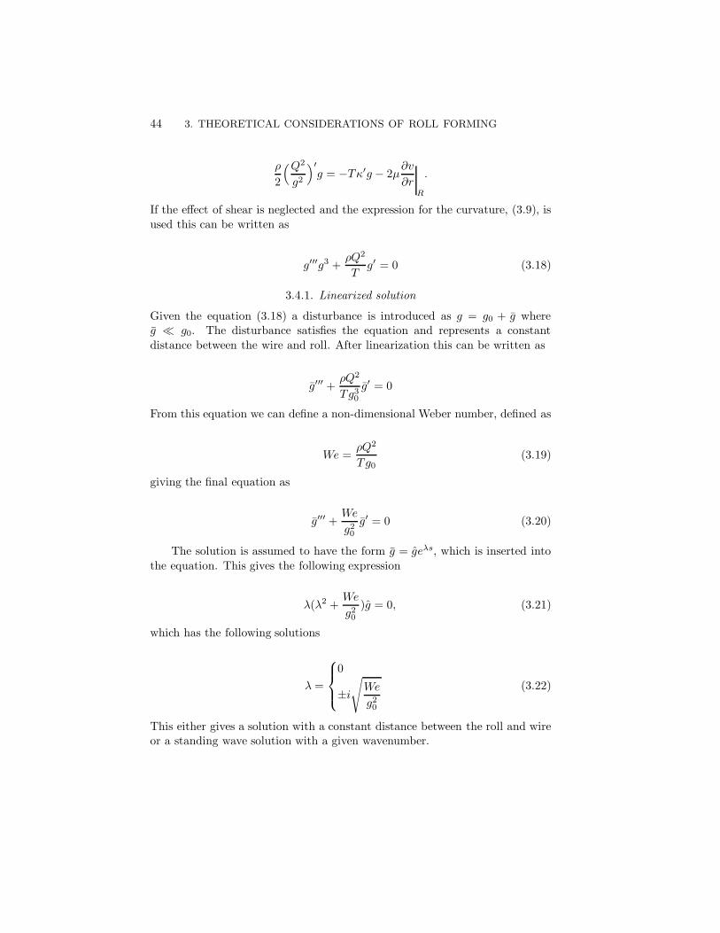
Results
In this chapter the results obtained with the KTH-former are presented. Mea-surements of the pressure and wire position in the roll forming zone are pre-sented for the three different permeabilities used in the study (non-permeable,semi-permeable and open/conventional wire). The results are obtained at dif-ferent nominal dewatering pressures p = T/R (see chapter 3), i.e. the wiretension is varied. In general, the dynamic pressure in the water jet and thedewatering pressure are the important quantities. If the available momentum(dynamic pressure) of the jet is too low compared to the dewatering pressurethe fluid will not be able to pass through the dewatering zone. At an earlierstage, at a nominal pressure approximately half of the dynamic pressure, sur-face ripples are seen on the water jet at impingement. If the nominal pressureis increased even more the ripples will grow to a chaotic air-water mixtureswirling on the water jet surface. This chaotic entry will be referred to as thecollapse case.
The results from the three different wires are presented and compared inthe first section of this chapter. In the second section, the results obtainedwith the non- and semi-permeable wires are studied in detail. In all thosecases the roll mounted pressure transducer was used. Additionally, for thenon-permeable wire case, results obtained with the trailing Samba sensor arepresented. In the last section the measured dewatering/drainage rates for thesemi-permeable wire case are presented.
The standard experimental condition was a flow rate of 450 l/min and aheight of the headbox nozzle of 12 mm. This corresponds to a jet speed of6.25 m/s. The wire speed was set to the same value, so there was no speeddifference between the jet and the wire.
4.1. Overview of pressure and wire position
In the following we will show results from the pressure measurements in theform of the unscaled pressure in kPa as a function of the normalised wrapangle ϕ = wrap angle/2π. The zero point for the wrap angle represent thetriggering point position as described in section 2.3 Measurements techniques.
45

46 4. RESULTS
0.05 0.1 0.15 0.2 0.25-30
-25
-20
-15
-10
-5
0
5
10
15
Pre
ssur
e [k
Pa]
Normalised wrap angle
4.2 kPa4.95.57.27.5
Figure 4.1. Roll pressure at different nominal pressure forthe non-permeable wire case.
In all cases, the curves shown are the result of ensemble averaging of (typically)ten consecutive measurements in the roll forming zone.
Non-permeable wire case
The pressure measurement results for the non-permeable wire case are shownin figure 4.1. From the graph, which shows five different nominal pressuresin the range 4.2–7.5 kPa, it is clear that the behaviour for all cases is simi-lar. Initially there is a pressure build up, which is followed by a decrease inpressure, whereafter a new pressure build up is seen. The first peak reachesapproximately the nominal pressure T/R, whereas the second peak reaches aneven higher value. The local minimum between the two pressure peaks are forall cases significantly below zero.
The length of the pressure event is strongly related to the value of thenominal pressure. By inspection of figure 4.1, it is clear that the first peak andthe minimum shift upstream when the wire tension is increased. At the end ofthe pressure event there is a very distinct suction peak, which is located in theregion where the wire is pulled away from the roll surface.
From visual observations the flow in the region where the wire separatesfrom the roll appears to be chaotic and there is a water spray exiting at the

4.1. OVERVIEW OF PRESSURE AND WIRE POSITION 47
Rol
l-wire
dis
tanc
e
0.06
0.13
0.19
0.25Roll4.2 kPa4.95.57.27.5
Possible wire path at 7.5 kPa
Figure 4.2. Wire position for five different nominal pressuresin a cartesian coordinate system. Note that the dashed linecorresponds to the outer measurement range of the positiontransducer and the dotted line to a possible wire path for the7.5 kPa case.
roll-wire separation point. It seems that the water is mainly transported alongthe roll surface after the wire has separated from the roll. The spray is probablya result of the centrifugal effects, which force the water to be thrown off theroll. The spray did not have a uniform structure in the spanwise directionbut seemed to be more pronounced at the middle of the roll. Because of therange and characteristics of the pressure transducer the quantitative value ofthe suction peak is questionable. However, the presence of it and its positionis believed to be correct.
The wire position for the same cases as in figure 4.1 is shown in figure 4.2in a cartesian coordinate system. The roll surface is visible as the thick solidcurve and radial rays indicate the corresponding normalized wrap angle. For allnominal pressures the curves seem to fall on top of each other except for the onewith the highest nominal pressure. This case represents the collapse case, notmeaning a wire collapse on the roll surface but an impingement zone collapsewhen the nominal pressure reach 40% of the dynamic water jet pressure. Atthe entrance and exit the wire seems to enter and leave tangentially to the roll.
The measured wire position can be compared to the photo in figure 4.3.This photo shows the dewatering zone from the side and the geometry is similar

48 4. RESULTS
Figure 4.3. The wire position at running conditions, the im-pingement zone to the left and wire separation in the upperright corner.
to what is shown in the graph in figure 4.2. The water jet and the impingementzone can be seen to the left and the separation zone can be found in the upperright corner. In the photo the roll and the wire can be clearly seen at theentrance and at the exit. In the dewatering zone the wire shape could befollowed as its curvature varied relative to the overall curvature due to the rollradius. Just prior to the wire separation the wire is closest to the roll whichcan also be seen in figure 4.2.
The wire position (in mm from the roll surface) for the same cases asin figure 4.1 is shown in figure 4.4, except for the highest nominal pressure.Also shown as a reference is the no-water case together with the correspondinganalytical solution, from section 2.3.2Wire position measurements. The entryand exit trajectories are seen to follow that of the geometrical expression well.The figure also shows the fact that the transducer was radially displaced toincrease the measuring range and that the positioning pin, with a stroke of 13mm, was mounted with an offset of 5 mm in this case.
For all cases with water the entrance region is displaced from the analyticalexpression but has the same shape. This shift is caused by the displacementof the wire due to the entering water jet. Since all cases, independent of thenominal pressure, initially follow the same trajectory it does not seem that thejet momentum deflects the wire, but instead this displacement depends on theflow rate, i.e. the amount of water that pass the dewatering zone.
The dewatering zone can be defined as the region where the shape of thewire start to diverge from the analytical no-water case (ϕ=0.07) until the wire-roll distance becomes a minimum (ϕ=0.22). In this case it corresponds to awrap length of 310 mm.
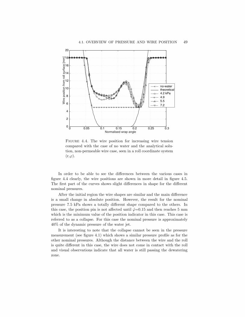
4.1. OVERVIEW OF PRESSURE AND WIRE POSITION 49
0 0.05 0.1 0.15 0.2 0.25 0.30
2
4
6
8
10
12
14
16
18
20
no-watertheoretical4.2 kPa4.95.57.2
Normalised wrap angle
Wire
pos
ition
from
rol
l sur
face
[mm
]
Figure 4.4. The wire position for increasing wire tensioncompared with the case of no water and the analytical solu-tion, non-permeable wire case, seen in a roll coordinate system(r,ϕ).
In order to be able to see the differences between the various cases infigure 4.4 clearly, the wire positions are shown in more detail in figure 4.5.The first part of the curves shows slight differences in shape for the differentnominal pressures.
After the initial region the wire shapes are similar and the main differenceis a small change in absolute position. However, the result for the nominalpressure 7.5 kPa shows a totally different shape compared to the others. Inthis case, the position pin is not affected until ϕ=0.15 and then reaches 5 mmwhich is the minimum value of the position indicator in this case. This case isreferred to as a collapse. For this case the nominal pressure is approximately40% of the dynamic pressure of the water jet.
It is interesting to note that the collapse cannot be seen in the pressuremeasurement (see figure 4.1) which shows a similar pressure profile as for theother nominal pressures. Although the distance between the wire and the rollis quite different in this case, the wire does not come in contact with the rolland visual observations indicate that all water is still passing the dewateringzone.

50 4. RESULTS
0.05 0.1 0.15 0.2 0.250
5
10
15
Wire
pos
ition
[mm
]
Normalised wrap angle
4.2 kPa4.95.57.27.5
Figure 4.5. Wire position at different nominal pressures,close up.
Semi-permeable wire case
The corresponding pressure measurement results for the semi-permeable wirecase is seen in figure 4.6. Also in this case two pressure peaks appear as wellas a suction peak at separation. The peak values increase with increasingnominal pressure. The 4.2 kPa case shows a very gentle build up and reachesits maximum pressure just prior to separation. At ϕ=0.14 a local pressureminimum can be detected, but not as obvious as for the other cases. In the 7.5kPa and 7.9 kPa case, the second peak becomes dominant and the first peakis partly merged into the second one. The local pressure minimum in betweenthe two positive peaks stays positive in almost all cases, and the suction peaksat the point of separation are fairly independent of the nominal pressure.
After the suction peak, ϕ >0.21, a negative pressure is registered. Thismay be due to the water that is transported along the roll after wire separation.However, the magnitude is unrealistic and this delay in the recovery after thesuction peak is attributed to the characteristics of the pressure transducer. Thetransducer, unfortunately, showed different response time for recovery fromnegative and from positive pressure, see section 2.3.1 Pressure measurements.
In figure 4.7 the results for the wire position is shown. The variation inthe position for the different nominal pressures is larger in the second partthan in the first part. At mid section, at approximately ϕ=0.17, the wire has a
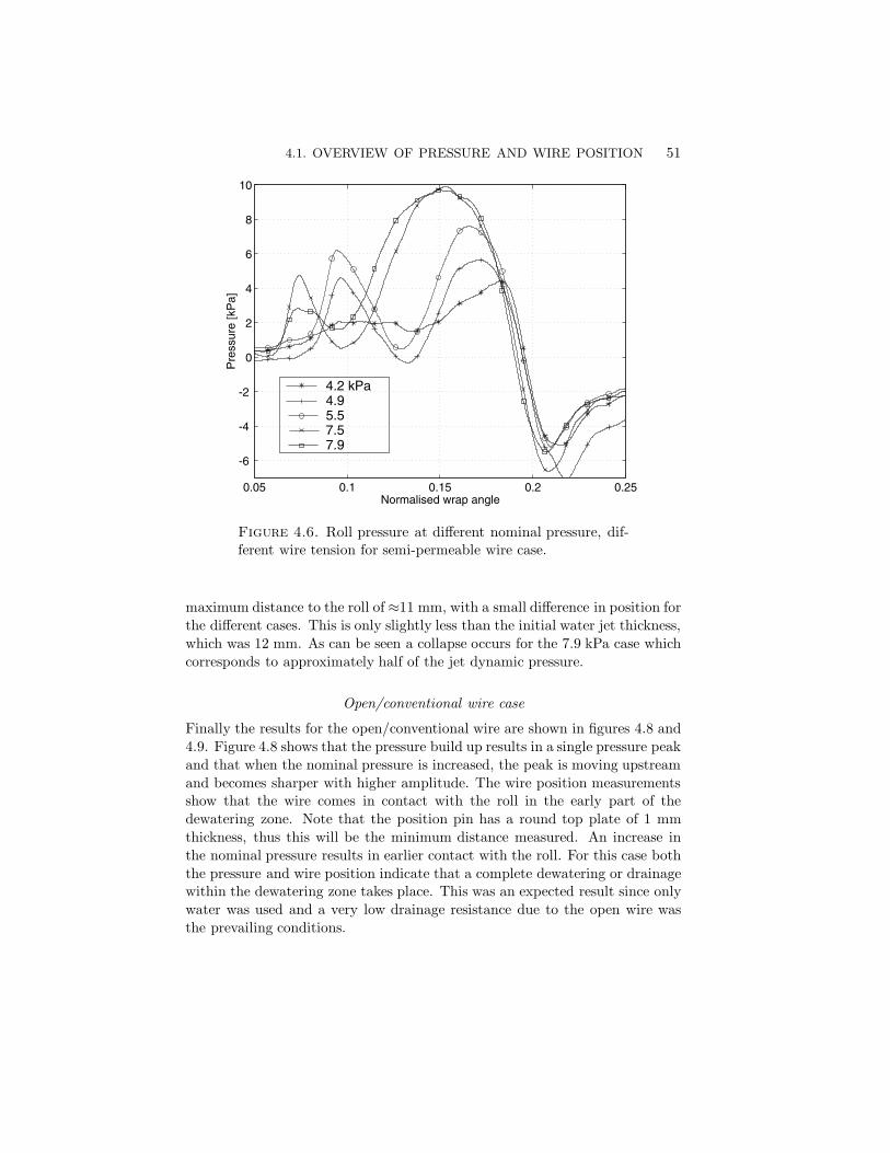
4.1. OVERVIEW OF PRESSURE AND WIRE POSITION 51
0.05 0.1 0.15 0.2 0.25
-6
-4
-2
0
2
4
6
8
10
Pre
ssur
e [k
Pa]
Normalised wrap angle
4.2 kPa4.95.57.57.9
Figure 4.6. Roll pressure at different nominal pressure, dif-ferent wire tension for semi-permeable wire case.
maximum distance to the roll of ≈11 mm, with a small difference in position forthe different cases. This is only slightly less than the initial water jet thickness,which was 12 mm. As can be seen a collapse occurs for the 7.9 kPa case whichcorresponds to approximately half of the jet dynamic pressure.
Open/conventional wire case
Finally the results for the open/conventional wire are shown in figures 4.8 and4.9. Figure 4.8 shows that the pressure build up results in a single pressure peakand that when the nominal pressure is increased, the peak is moving upstreamand becomes sharper with higher amplitude. The wire position measurementsshow that the wire comes in contact with the roll in the early part of thedewatering zone. Note that the position pin has a round top plate of 1 mmthickness, thus this will be the minimum distance measured. An increase inthe nominal pressure results in earlier contact with the roll. For this case boththe pressure and wire position indicate that a complete dewatering or drainagewithin the dewatering zone takes place. This was an expected result since onlywater was used and a very low drainage resistance due to the open wire wasthe prevailing conditions.
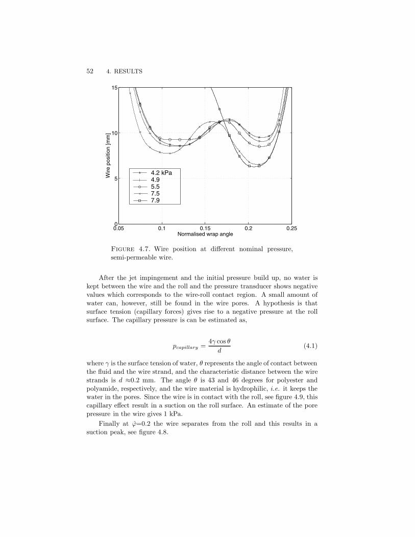
52 4. RESULTS
0.05 0.1 0.15 0.2 0.250
5
10
15
Wire
pos
ition
[mm
]
Normalised wrap angle
4.2 kPa4.95.57.57.9
Figure 4.7. Wire position at different nominal pressure,semi-permeable wire.
After the jet impingement and the initial pressure build up, no water iskept between the wire and the roll and the pressure transducer shows negativevalues which corresponds to the wire-roll contact region. A small amount ofwater can, however, still be found in the wire pores. A hypothesis is thatsurface tension (capillary forces) gives rise to a negative pressure at the rollsurface. The capillary pressure is can be estimated as,
pcapillary =4γ cos θ
d(4.1)
where γ is the surface tension of water, θ represents the angle of contact betweenthe fluid and the wire strand, and the characteristic distance between the wirestrands is d ≈0.2 mm. The angle θ is 43 and 46 degrees for polyester andpolyamide, respectively, and the wire material is hydrophilic, i.e. it keeps thewater in the pores. Since the wire is in contact with the roll, see figure 4.9, thiscapillary effect result in a suction on the roll surface. An estimate of the porepressure in the wire gives 1 kPa.
Finally at ϕ=0.2 the wire separates from the roll and this results in asuction peak, see figure 4.8.

4.2. DETAILED STUDY OF PRESSURE AND WIRE POSITION 53
0.05 0.1 0.15 0.2 0.25-3
-2
-1
0
1
2
3
4
5
6
Pre
ssur
e [k
Pa]
Normalised wrap angle
4.2 kPa4.95.57.57.9
Figure 4.8. Roll pressure at different different nominal pres-sure for the conventional wire case
4.2. Detailed study of pressure and wire position
4.2.1. Non-permeable wire case
In this section a detailed analysis of the results obtained with the non-permeablewire is presented. This is done for three nominal pressures (4.7 kPa, 5.4 kPa,7 kPa) by varying the wire tension.
In figure 4.10, the pressures and the wire positions are compared for thedifferent cases. For the nominal pressure 4.7 kPa, the upper left figure, thefirst peak approximately reaches the nominal value (T/R), whereas the secondpeak reaches an even higher value (9 kPa). The corresponding wire positioncurve rapidly reaches a “plateau” in the first half. After this it increases to apeak that is positioned after the pressure peak and finally leaves the roll at alevel of approximately 5.5 mm.
The 5.4 kPa-case shows a pressure curve which is much more symmetricthan in the 4.7 kPa-case. Also, the amplitude of the first pressure peak isalmost as high as for the second peak. If the first part of the position curve iscompared to the 4.7 kPa case there seems to be one more inflection point.

54 4. RESULTS
0.05 0.1 0.15 0.2 0.250
1
2
3
4
5
6
7
8
9
10
Wire
pos
ition
[mm
]
Normalised wrap angle
4.2 kPa4.95.57.57.9
Figure 4.9. Wire position at different nominal pressure forthe conventional wire case.
For the 7 kPa case there is a very good agreement between the pressurepeaks and extreme points of the wire position which later will be shown tocorrelate to the local curvature.
In the bottom-left graph in figure 4.10 a comparison between the positioncurves for the different wire tensions can be seen. These show a similar shapealthough there are some minor differences in shape. The maximum distancecan be found at ϕ=0.17, where the roll-wire distance is 11–12 mm.
If the pressure curves are compared it is obvious that the coupling of thesecond peak to the nominal pressure is weak. The suction peak at separationis apparently much larger than the pressure peak. The suction does not appearin a predictable way with changing wire tension. Since the amplitude is notreliable due to the characteristics of the transducer, no further conclusions arehowever drawn.
A comparison between the pressure and position curves gives a fairly goodagreement with a maximum in wire position at the point of maximum in pres-sure. If the three cases are compared there is a shift of ϕ=0.03 in the maximumpressure peak, which cannot be seen in the wire position. This may be due tothat also small changes in position may result in a large change in the pressure,
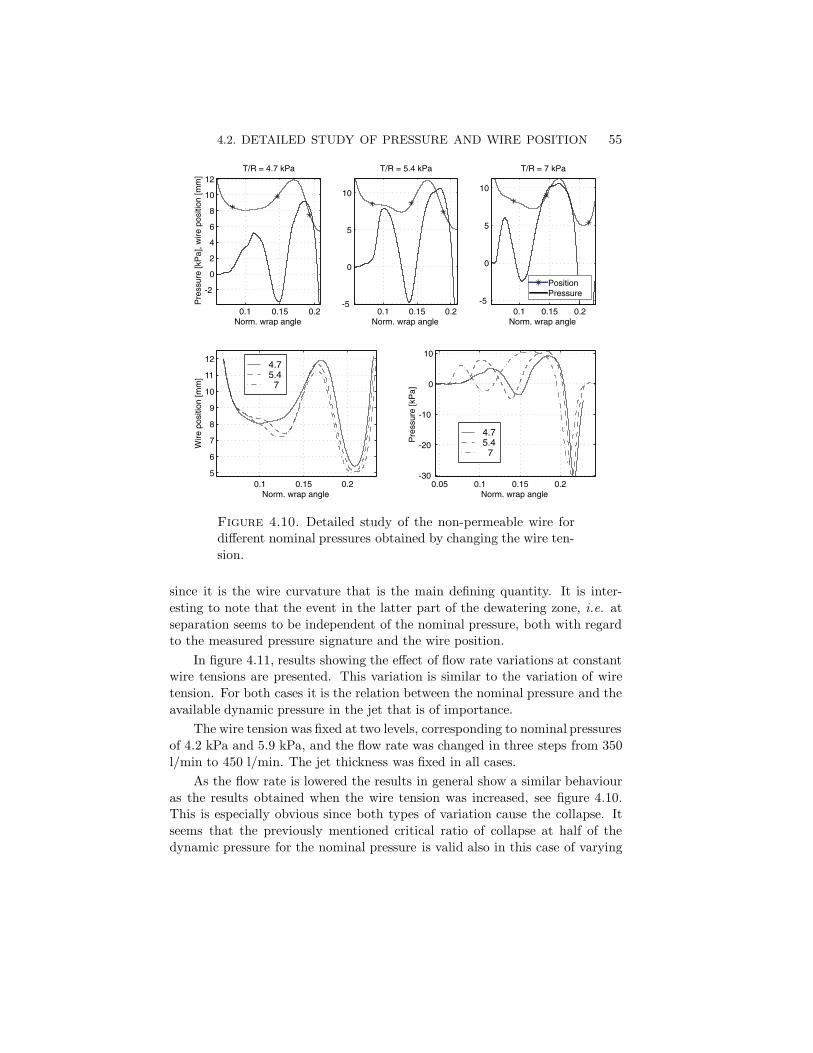
4.2. DETAILED STUDY OF PRESSURE AND WIRE POSITION 55
0.1 0.15 0.2
-2
0
2
4
6
8
10
12T/R = 4.7 kPa
Pre
ssur
e [k
Pa]
, wire
pos
ition
[mm
]
Norm. wrap angle
0.1 0.15 0.25
6
7
8
9
10
11
12
Wire
pos
ition
[mm
]
Norm. wrap angle 0.05 0.1 0.15 0.2
-30
-20
-10
0
10
Pre
ssur
e [k
Pa]
Norm. wrap angle
0.1 0.15 0.2-5
0
5
10
T/R = 5.4 kPa
Norm. wrap angle 0.1 0.15 0.2
-5
0
5
10
T/R = 7 kPa
Norm. wrap angle
4.75.4 7
4.75.4 7
PositionPressure
Figure 4.10. Detailed study of the non-permeable wire fordifferent nominal pressures obtained by changing the wire ten-sion.
since it is the wire curvature that is the main defining quantity. It is inter-esting to note that the event in the latter part of the dewatering zone, i.e. atseparation seems to be independent of the nominal pressure, both with regardto the measured pressure signature and the wire position.
In figure 4.11, results showing the effect of flow rate variations at constantwire tensions are presented. This variation is similar to the variation of wiretension. For both cases it is the relation between the nominal pressure and theavailable dynamic pressure in the jet that is of importance.
The wire tension was fixed at two levels, corresponding to nominal pressuresof 4.2 kPa and 5.9 kPa, and the flow rate was changed in three steps from 350l/min to 450 l/min. The jet thickness was fixed in all cases.
As the flow rate is lowered the results in general show a similar behaviouras the results obtained when the wire tension was increased, see figure 4.10.This is especially obvious since both types of variation cause the collapse. Itseems that the previously mentioned critical ratio of collapse at half of thedynamic pressure for the nominal pressure is valid also in this case of varying

56 4. RESULTS
0.05 0.1 0.15 0.2-30
-20
-10
0
10
Pre
ssur
e [k
Pa]
Norm. wrap angle
Flow = 450 l/min
0.05 0.1 0.15 0.2 0.25-30
-20
-10
0
10
T/R = 4.2kPa
Norm. wrap angle
Pre
ssur
e [k
Pa]
0.05 0.1 0.15 0.2-30
-20
-10
0
10
Flow = 400 l/min
Norm. wrap angle0.05 0.1 0.15 0.2
-30
-20
-10
0
10
Flow = 350 l/min
Norm. wrap angle
0.05 0.1 0.15 0.2 0.25-30
-20
-10
0
10
T/R = 5.9kPa
Norm. wrap angle
450 l/min400350
450 l/min400350
T/R= 4.2 kPaT/R= 5.9 kPa
Figure 4.11. The pressure signature for the non-permeablewire. The wire tension was fixed at two levels, correspondingto the nominal pressure of 4.2 kPa and 5.9 kPa and the flowrate was changed in three steps from 350 l/min to 450 l/min.The jet thickness was fixed in all cases.
the flow rate. For cases close to collapse the pressure amplitude is reducedand in the case of 5.9 kPa and 350 l/min the collapse is evident from visualobservations.
Pressure measurements were also carried out with the water jet trailingtransducer, i.e. the Samba sensor. Unfortunately, the dynamics in the form-ing roll pressure transducer failed in this test but the wire position data wasstill reliable. As a consequence of this, the only direct comparison of the twodifferent pressure measurement methods was carried out by keeping the roll atone position while the outer-wire and jet was still running. The pressure wasthen measured with the pressure transducer in the roll at one static position,see figure 4.12. This was repeated for 30 positions with 10 mm spacing in thedewatering zone. Simultaneously, the Samba sensor was used and a comparisonwas possible. This procedure was only possible at low nominal pressure, in theother cases the collapse was very close, closer than when the roll was rotating.

4.2. DETAILED STUDY OF PRESSURE AND WIRE POSITION 57
0.08 0.1 0.12 0.14 0.16 0.18 0.2 0.22-6
-4
-2
0
2
4
6
8
Pre
ssur
e [k
Pa]
Normalised wrap angle
Samba sensorRoll transducer
Figure 4.12. Samba sensor and forming roll transducer atdifferent positions in the dewatering zone, static measurementsat a nominal pressure of 3.5 kPa, the non-permeable wire case.
The results obtained with the Samba sensor show similar pressure profilesas those which have been presented earlier, see figure 4.12. A pressure buildup in the initial part is followed by a local pressure minimum in the region ofϕ=0.11. The second pressure peak reaches its maximum just prior to the exit.As mentioned in section 2.3 Measurements techniques, measurements at thesuction peak were not possible. The two static pressure measurement methodsshown in the figure indicate that the Samba sensor registers a higher pressurethan the transducer mounted in the roll. The difference between the recordedpressures is the centrifugal pressure, which can be estimated to approximately2 kPa.
In these tests the wrap angle was decreased with 20% (250 mm) comparedto the earlier presented results. However, no significant changes in the pressurecharacteristics was seen. This indicates only marginal effects of the wrap angleon the dewatering pressure and wire position.
The Samba sensor pressure and the wire position are shown in figure 4.13during normal rotating conditions. The discrete points (10 mm spacing) fromthe measurements are complemented by a polynomial curvefit.
4.2.2. Semi-permeable wire case
Figure 4.14 shows the pressure and the wire position for the semi-permeablewire case for three nominal pressures (4.2 kPa, 5.9 kPa and 7.5 kPa). Allthree cases show increasing pressure amplitudes for increasing nominal pressure.Also, the pressure minimum is positive for all cases. The second pressure peak

58 4. RESULTS
0.06 0.08 0.1 0.12 0.14 0.16 0.18 0.20
2
4
6
8
10
12
Pre
ssur
e [k
Pa]
, wire
pos
ition
[mm
]
Normalised wrap angle
Samba dataCurvfit to the dataWire position
Figure 4.13. Samba sensor pressure measurements and wireposition, a nominal pressure of 4.5 kPa, non-permeable wire.
amplitude changes significantly (from 4 kPa to 9.5 kPa) with increasing nominalpressure. The suction peak was reduced compared to the non-permeable caseand was approximately the same order as the obtained dewatering pressure.The pressure and the wire position seems to correlate well for all three cases.
In the lower left graph in figure 4.14 a comparison between the three wireposition curves shows a difference compared to the case with the non-permeablewire. More of less the entire wire position curve changes with different nominalpressure. Also, the minimum value of the wire position, at ϕ=0.2, varied withthe nominal pressure.
It seems that the reduced suction peak results in a dewatering case, thatis more sensitive to the changes in wire tension. An increase in the nominalpressure resulted in a higher pressure peak. Thus, higher dewatering pressureresulted in a reduced wire-roll distance.
The variation of flow rate, figure 4.15, gave similar results as the onesobtained with the non-permeable wire. The wire tension was fixed at twolevels, corresponding to the nominal pressure of 4.2 kPa and 5.9 kPa and theflow rate was changed in three steps from 350 l/min to 450 l/min. The jetthickness was fixed in all cases. However, the local pressure minimum betweenϕ=0.1–0.15 shows a negative value as the flow rate is decreasing just beforecollapse. This is a difference from the results with varying wire tension whereno negative values were found.

4.2. DETAILED STUDY OF PRESSURE AND WIRE POSITION 59
0.1 0.15 0.2
0
5
10
15
T/R = 4.2 kPa
Pre
ssur
e [k
Pa]
, wire
pos
ition
[mm
]
Norm. wrap angle
0.1 0.15 0.2
6
8
10
12
14
Wire
pos
ition
[mm
]
Norm. wrap angle 0.1 0.15 0.2
-6
-4
-2
0
2
4
6
8
Pre
ssur
e [k
Pa]
Norm. wrap angle
0.1 0.15 0.2
0
5
10
T/R = 5.9 kPa
Norm. wrap angle 0.1 0.15 0.2
-5
0
5
10
T/R = 7.5 kPa
Norm. wrap angle
4.25.97.5
4.25.97.5
PositionPressure
Figure 4.14. Detailed study of semi-permeable wire case fordifferent nominal pressures obtained by changing the wire ten-sion.
4.2.3. Non-permeable and semi-permeable wire case
The results obtained with the non-permeable and the semi-permeable wires,see figure 4.16, show similar features. The two cases are shown for two nominalpressures (4.9 kPa and 7.2 kPa). The agreement is very good, although theyrepresent two different cases, no dewatering and dewatering. A difference canbe seen in the suction peak at separation, where the suction certainly causethe wire to come closer to the roll, which is seen in the lower left plot in fig-ure 4.16. By changing the wire tension the shift upstream in the pressure isvisible for both wire cases. For the semi-permeable wire the pressure ampli-tude seems to follow the nominal pressure whereas for the non-permeable itis always at a high level. The significant pressure minimum at the midsectionof the dewatering zone (ϕ=0.10–0.15) in the non-permeable case is due to thecentrifugal pressure which is reduced in the semi-permeable wire case. This isdue to the fundamental difference implied by the presence of drainage in thesemi-permeable wire case.

60 4. RESULTS
0.05 0.1 0.15 0.2
-6
-4
-2
0
2
4
6P
ress
ure
[kP
a]
Norm. wrap angle
Flow = 450 l/min
0.05 0.1 0.15 0.2 0.25
-6
-4
-2
0
2
4
6
T/R = 4.2 kPa
Norm. wrap angle
Pre
ssur
e [k
Pa]
0.05 0.1 0.15 0.2
-6
-4
-2
0
2
4
6
Flow = 400 l/min
Norm. wrap angle0.05 0.1 0.15 0.2
-6
-4
-2
0
2
4
6
Flow = 350 l/min
Norm. wrap angle
0.05 0.1 0.15 0.2 0.25
-6
-4
-2
0
2
4
6
T/R = 5.9 kPa
Norm. wrap angle
T/R= 4.2 kPaT/R= 5.9 kPa
450 l/min400350
450 l/min400350
Figure 4.15. The pressure signature for semi-permeablewire. The wire tension was fixed at two levels, correspond-ing to the nominal pressure of 4.2 kPa and 5.9 kPa and theflow rate was changed in three steps from 350 l/min to 450l/min. The jet thickness was fixed in all cases.
For the semi-permeable wire both the wire position and the pressure ischanged with different nominal pressures, whereas this effect is marginal forthe non-permeable wire. This may be due to the very pronounced suction peakrecorded at separation in the non-permeable wire case. The wire position ismarginally shifted as the nominal pressure is changed in the non-permeablecase where the suction peak is more than 4 times higher. The difference of thesuction peak is most likely due to the drainage possibilities.
As was seen in figure 4.6, a higher nominal pressure before collapse (7.9kPa) is reached for the semi-permeable case than for the non-permeable case(7.5 kPa). Consequently, the drainage seems to have a stabilising effect butnot necessarily a large influence on the characteristics.

4.3. LOCAL DRAINAGE MEASUREMENTS 61
0.05 0.1 0.15 0.2 0.25-30
-20
-10
0
10
Norm. wrap angle
Pre
ssur
e [k
Pa]
T/R = 4.9 kPa
0.05 0.1 0.15 0.2 0.25
6
8
10
12
Norm. wrap angle
Wire
pos
ition
[mm
]
0.05 0.1 0.15 0.2 0.25-30
-20
-10
0
10
Norm. wrap angle
Pre
ssur
e [k
Pa]
T/R = 7.2 kPa
0.05 0.1 0.15 0.2 0.25
6
8
10
12
Norm. wrap angle
Wire
pos
ition
[mm
]
Semi-perm wireNon-perm wire
Figure 4.16. Non-permeable and semi-permeable wire case,the pressure and wire position for two different nominal pres-sure, 4.9 and 7.2 kPa
4.3. Local drainage measurements
The arrangement to make local drainage measurements was described in chap-ter 2, where the saveall arrangement was described. Such measurements weremade both with pure water and with fibre suspensions, but only the formerare reported here. The present measurements were carried out for the semi-permeable case at a nominal pressure of 5.9 kPa. The measurements withthe saveall was a time consuming procedure, during which the system waschallenged when keeping a constant flow of 400 l/min. The results of thesemeasurements are shown in figure 4.17. Included are three different sets ofmeasurements which give an idea of the repeatability of the method. The dis-crepancies in the overlapping position (i+ 1) of upstream saveall and position(i) of the downstream saveall show the difficulties to adjust the saveall. Thesaveall had to be sufficiently close to the wire to collect the expelled waterwithout influencing the wire.
As can be seen the drainage measurements also give distributions with twopeaks, which are similar to the pressure results. An initial increase is followed

62 4. RESULTS
0.06 0.08 0.1 0.12 0.14 0.16 0.18
0.2
0.4
0.6
0.8
1
1.2
Normalised wrap angle
Dra
inag
e ra
te [l
/min
]
upstream savealldownstream saveall
Figure 4.17. Drainage measurements along the dewateringzone using the double box collector for the semi-permeablewire. Three different sets of measurements from the upstreamand downstream collector boxes. Nominal pressure 5.9 kPaand flow rate 400 l/min.
0.05 0.1 0.15 0.2-6
-4
-2
0
2
4
6
8
10
12
14
Normalised wrap angleNormalised wrap angle
Pre
ssur
e [k
Pa]
, Wire
pos
ition
[mm
]
0.1
0.2
0.3
0.4
0.5
0.6
0.7
0.8
0.9
1
1.1D
rain
age
rate
[l/m
in]
PressurePositionDrainage
Figure 4.18. The measured pressure and wire position withthe corresponding drainage rate, average data from figure 4.17.
by a minimum at around ϕ=0.12 and finally an increase at the end of thedewatering zone. The second peak is smaller than the first, which is oppositeto the corresponding pressure measurements.

4.3. LOCAL DRAINAGE MEASUREMENTS 63
The mean drainage rate, averaged from the measurements in figure 4.17is shown together with the corresponding pressure and wire position in figure4.18.
The result from the saveall measurements showed that approximately 30 %of the total flow was drained within the dewatering zone. This means that asubstantial amount of the water passes through the dewatering zone, so thiscase can indeed be described as partial dewatering.

64 4. RESULTS
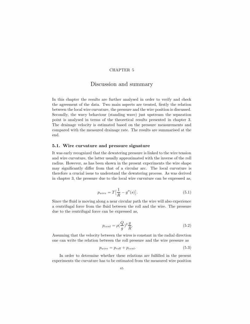
CHAPTER 5
Discussion and summary
In this chapter the results are further analysed in order to verify and checkthe agreement of the data. Two main aspects are treated, firstly the relationbetween the local wire curvature, the pressure and the wire position is discussed.Secondly, the wavy behaviour (standing wave) just upstream the separationpoint is analysed in terms of the theoretical results presented in chapter 3.The drainage velocity is estimated based on the pressure measurements andcompared with the measured drainage rate. The results are summarised at theend.
5.1. Wire curvature and pressure signature
It was early recognized that the dewatering pressure is linked to the wire tensionand wire curvature, the latter usually approximated with the inverse of the rollradius. However, as has been shown in the present experiments the wire shapemay significantly differ from that of a circular arc. The local curvature istherefore a crucial issue to understand the dewatering process. As was derivedin chapter 3, the pressure due to the local wire curvature can be expressed as,
pwire = T[ 1R
− g′′(s)]. (5.1)
Since the fluid is moving along a near circular path the wire will also experiencea centrifugal force from the fluid between the roll and the wire. The pressuredue to the centrifugal force can be expressed as,
pcent = ρ(Q
g)2g
R. (5.2)
Assuming that the velocity between the wires is constant in the radial directionone can write the relation between the roll pressure and the wire pressure as
pwire = proll + pcent. (5.3)
In order to determine whether these relations are fulfilled in the presentexperiments the curvature has to be estimated from the measured wire position
65

66 5. DISCUSSION AND SUMMARY
data. The estimate is made by fitting an 8th degree polynomial to the measuredwire position data. The pressure, wire position and estimated curvature areshown in figure 5.1 for the non-permeable wire case at a nominal pressure of5.4 kPa. When the wire is at a constant distance from the roll, the curvaturereduces to 1/(R+g), which is close to that of the roll (1/R). The roll curvatureis referred to as the nominal curvature and is 3.1 m−1. Although the curvaturevaries around the nominal value, the curvature remains positive, unless g′′R >
1.
0.08 0.1 0.12 0.14 0.16 0.18 0.2-10
-5
0
5
10
Norm. wrap angle
CurvaturePressure, [kPa]Wire position, [mm]Centrifugal pressure, [kPa]
Figure 5.1. The estimated curvature and the centrifugalpressure based on the measured wire position. The measuredroll pressure is also shown. The non-permeable wire case withnominal pressure (T/R) 5.4 kPa. In the present case the flowrate is 450 l/min.
As can be seen in figure 5.1 the curvature may well be above or belowthe nominal curvature. It can also be seen, that the shape of the plottedcurvature correlates well with the pressure distribution except at the entry andthe exit of the dewatering zone. At ϕ=0.14 the curvature has a minimumvalue close to zero and at ϕ=0.17 it reaches its maximum of 7.4 m−1. Atthe nominal pressure of 5.4 kPa, which corresponds to a wire tension of 1.76kN/m, these curvatures would yield pressures of approximately zero and 13kPa, respectively. However, the values measured by the roll transducer were-5 kPa and 10.5 kPa, although the magnitude of the negative pressure is notreliable due to the response characteristics of the pressure transducer. Animportant feature to explain the difference between the measured pressuresand the estimated ones is the centrifugal effect. According to equation (5.2),

5.2. CONSISTENCY OF PRESSURE AND WIRE POSITION DATA 67
the centrifugal pressure is fairly constant in the dewatering zone, approximately2 kPa (see figure 5.1). It follows from the relation (5.3) that the centrifugalpressure should be subtracted from the pressure calculated by the curvaturein order to give the roll pressure. Recalculated in this way, the agreementbetween the measured and the estimated roll pressure is rather good for thesecond peak whereas, for the first peak, the estimated values are too small.At the position of minimum curvature, the centrifugal forces should yield anegative roll pressure.1
Curvature helps us to understand the pressure distributions shown in figure4.1 for the case of a non-permeable wire. When the wire is separating from theroll, the splitting of the remaining liquid layer creates a low pressure betweenthe wire and the roll. It is hypothesised that the suction will cause the wire tostay close to the roll for a longer distance than if no such film splitting effectoccurs. A consequence of this is a large negative curvature where the wireleaves for the supporting roll. As no dewatering is taking place for the non-permeable wire the thickness is rather constant regardless of the wire tension.Hence, the suction due to the film splitting is constant. It follows that a higherwire tension will cause the wire to leave earlier towards the supporting roll,and the (negative) curvature will be reduced as the wire tension increases.
It seems like the wire has to compensate for the negative curvature at theseparation by a larger positive curvature slightly upstream. This effect is alsoreduced as the wire tension increases. The situation bears some resemblanceto a negative curvature being generated by a blade pushing against the wire(see Zahrai (1997), paper 2).
The higher positive curvature at lower wire tensions will result in a fairlyconstant amplitude of the second pressure peak, as seen in figure 4.1. However,away from the separation point the pressure distribution shows the expectedinfluence of the wire tension, i.e. a lower tension results in a lower pressure.
In the semi-permeable wire case the film splitting is much less pronouncedas a consequence of the possibility of communication through the wire. Thisexplains the influence of the wire tension on the amplitude of the second pres-sure peak in the case of semi-permeable wire, see figure 4.6. A comparison ofthe two different wire types (non- and semi-permeable) is seen in figure 4.16 attwo nominal pressures.
5.2. Consistency of pressure and wire position data
One way of checking the consistency of the experimental data is to integratethe pressure data to determine the corresponding wire positions. The relationbetween the pressure and the position is given by equation (5.1).
1It should be noted that the roll radius in a real paper machine is roughly five times larger
than in the KTH-Former, although the machine speed is higher.
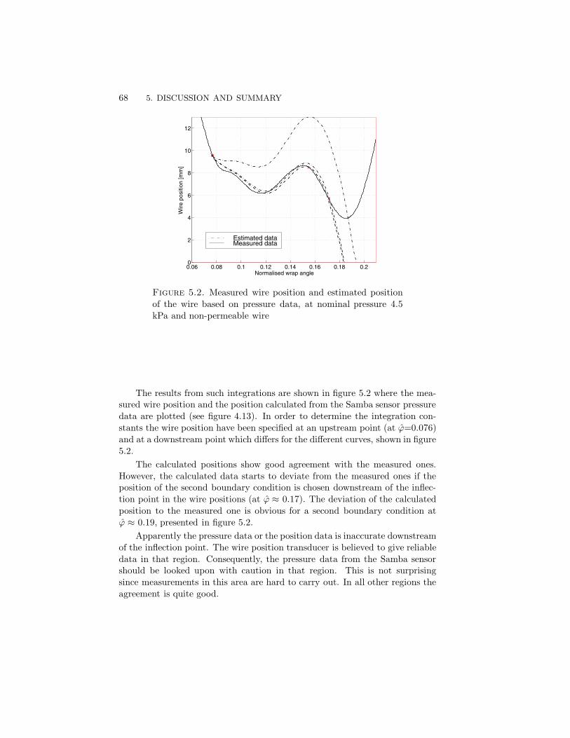
68 5. DISCUSSION AND SUMMARY
0.06 0.08 0.1 0.12 0.14 0.16 0.18 0.20
2
4
6
8
10
12
Wire
pos
ition
[mm
]
Normalised wrap angle
Estimated dataMeasured data
Figure 5.2. Measured wire position and estimated positionof the wire based on pressure data, at nominal pressure 4.5kPa and non-permeable wire
The results from such integrations are shown in figure 5.2 where the mea-sured wire position and the position calculated from the Samba sensor pressuredata are plotted (see figure 4.13). In order to determine the integration con-stants the wire position have been specified at an upstream point (at ϕ=0.076)and at a downstream point which differs for the different curves, shown in figure5.2.
The calculated positions show good agreement with the measured ones.However, the calculated data starts to deviate from the measured ones if theposition of the second boundary condition is chosen downstream of the inflec-tion point in the wire positions (at ϕ ≈ 0.17). The deviation of the calculatedposition to the measured one is obvious for a second boundary condition atϕ ≈ 0.19, presented in figure 5.2.
Apparently the pressure data or the position data is inaccurate downstreamof the inflection point. The wire position transducer is believed to give reliabledata in that region. Consequently, the pressure data from the Samba sensorshould be looked upon with caution in that region. This is not surprisingsince measurements in this area are hard to carry out. In all other regions theagreement is quite good.
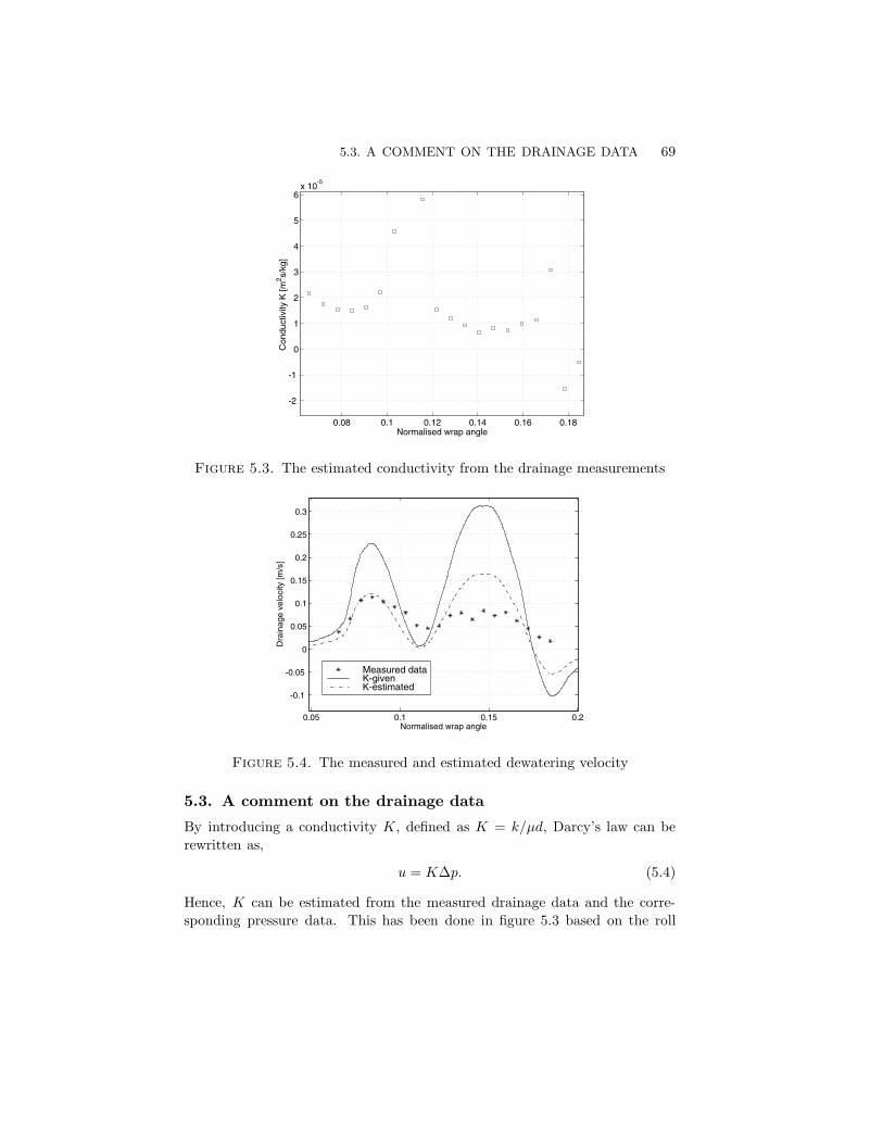
5.3. A COMMENT ON THE DRAINAGE DATA 69
0.08 0.1 0.12 0.14 0.16 0.18
-2
-1
0
1
2
3
4
5
6x 10
-5
Normalised wrap angle
Con
duct
ivity
K [m
2 s/kg
]
Figure 5.3. The estimated conductivity from the drainage measurements
0.05 0.1 0.15 0.2
-0.1
-0.05
0
0.05
0.1
0.15
0.2
0.25
0.3
Dra
inag
e ve
loci
ty [m
/s]
Normalised wrap angle
Measured dataK-givenK-estimated
Figure 5.4. The measured and estimated dewatering velocity
5.3. A comment on the drainage data
By introducing a conductivity K, defined as K = k/µd, Darcy’s law can berewritten as,
u = K∆p. (5.4)
Hence, K can be estimated from the measured drainage data and the corre-sponding pressure data. This has been done in figure 5.3 based on the roll
70 5. DISCUSSION AND SUMMARY
transducer data, with compensation for the centrifugal pressure according toequation (5.2). One value of K (at ϕ=0.116) have been excluded because it isunrealistic. The value correspond to a position where a dewatering has beenmeasured despite that the pressure was close to zero. An average over theaccepted values yields a K of 1.5 ·10−5m2s/kg.
In figure 5.4, the averaged K has been used to determine the drainagevelocities from the pressure measurements. As expected there is a reasonableagreement with the drainage results obtained directly from the measurements.
In the downstream region, the deviation becomes large due to the factthat the difference between the average K and ∆p/u is amplified when K ismultiplied with the high pressures there.
The permeability data for the semi-permeable wire measured as describedin chapter 2 results in K=3·10−5m2s/kg. Using the same pressure distributionas previously this would result in the drainage distribution, plotted as a solidcurve in figure 5.4. These drainage velocities seem reasonable in that they areof the same magnitude one would expect in a real paper machine for the samenominal pressure.
One may conclude that the experimental drainage velocities seem to betoo low. This is not surprising since it is difficult to do accurate measurementswith the saveall. However, the trend in the distribution has been captured. Therealistic values obtained when the wire data was used supports the credibilityof the pressure results.
5.4. The wire oscillatory behaviour
As the wire is taken off the roll a disturbance is introduced into the fluid-wire system. In chapter 3, it was shown that a disturbance may result inan oscillating solution for the wire position, and hence also for the pressuredistribution. Although the analysis was carried out for the non-permeable wire,such behaviour can also be expected for the semi-permeable wire. However, thefinite permeability may result in that the oscillations becomes smaller which issupported by the work of Zahrai (1997).
In figure 5.5 the non-dimensional wave number (normalized with the rollradius R) for the oscillations seen in the pressure signatures is plotted as afunction of the Weber number. The experimental wave numbers are determinedfrom the pressure data (figure 4.1), where the distance between the first andthe second pressure peak is taken to be one wavelength. All the parametersthat form the Weber number are known, except for the distance between theroll and the wire. This distance, g0, refers to the wire position around whichthe analytical solution has been linearized. The value of g0 has been chosento the position where the pressure equals the nominal pressure (T/R) reducedby the centrifugal pressure, see section 3.4 Roll forming theory. From a strict

5.5. SUMMARY 71
point of view, different values of g0 should be used for each experimental run.The point where to determine the distance is hard to find, but it seems that asufficiently accurate choice for all cases is 10 mm. This distance is also seen inthe wire position, see figure 4.5, around where the oscillations are seen. Thewire position amplitudes are a few millimeters which is fairly large comparedwith the assumed small oscillations around g0 assumed in the theory. Thetheory also assumes an infinite domain, whereas in the experiments only onewavelength can be observed in the dewatering zone. Despite these limitationsthe agreement is good and it can be experimentally concluded that the standingwave observed in the dewatering zone is of capillary origin.
500 600 700 800 900 1000 1100 12000
2
4
6
8
10
12
14
16
Weber number
Non
-dim
ensi
onal
wav
e nu
mbe
r
Theoretical resultExperimental result
Figure 5.5. Normalised wave number versus Weber numberfor the non-permeable wire case.
5.5. Summary
The present work deals with some aspects of the fluid mechanics of paper-making, more specifically partial dewatering during roll forming. The study ismainly experimental. Pressure, wire position and drainage measurements havebeen carried out in an experimental facility which models the roll forming zoneof a paper machine. The results can be summarised as follows:
72 5. DISCUSSION AND SUMMARY
• The local curvature of the wire is strongly correlated to the dewatering pres-sure.• At the separation point of the wire from the roll a strong suction peak isrecorded.• Upstream the separation point a standing wave on the wire is observed whichgives rise to an oscillating pressure. The origin of the wave is due to a capillaryeffect where the wire tension is the determining variable in a non-dimensionalWeber number.• If complete dewatering is achieved upstream the separation point there areno waves developing on the wire.• Local drainage measurements show a correlation to the dewatering pressureand hence to the wire curvature.
The reported data refers to pure water and for a complete understandingthe influence of the fibre and the fibre web need to be studied. Such tests couldbe done in a pilot paper machine e.g. in the EuroFEX at STFI in Stockholm.Further studies can also be carried out at different parameter settings, e.g. avariation of the impingement angle. It would also be valuable if the flow fieldbetween the roll and the wire could be numerically modelled, where also thewire permeability is taken into consideration.

Acknowledgements
This survey into the field of fluid mechanics would not be so interesting withoutthe support of my supervisor Prof. Henrik Alfredsson. He believes in my ideasand forms them into realistic plans with a guiding hand.
The author would like to thank Dr. Daniel Soderberg for his endless pa-tience of my never ending questions and Prof. Bo Norman for sharing me hisexcellent knowledge in the field of paper making. Also, Prof. Fritz Bark forhis enthusiasm of my work. The contact with the industry through Dr. LarsMartinsson at Albany International AB has brought a lot of industrial aspectsinto this work.
I would like to thank all my colleagues at ”Labbet” at the Departmentof Mechanics without you fluid mechanics would loose one dimension. I wantto thank Marcus Gallstedt and Ulf Landen for all help and ideas during thedesign of set up. Also, thank to the people at the Department of Pulp andPaper Chemistry Technology at KTH, where the ”dirty ” work was carriedout.
Finally I would deeply like to thank my family for all their support, loveand understanding, and foremost Mia.
Funding for this project has been through FaxenLaboratoriet at the Depart-ment of Mechanics, KTH with support from the industrial partners and VIN-NOVA, which is greatly acknowledged.
73

74 ACKNOWLEDGEMENTS
—— ♥ ——
References
Boxer, T., Dodson, C. & Sampson, W. 2000 Analytic solution to the martinez
dewatering equations for roll gap forners. J. Pulp and Paper Science 26, 391–394.
Chen, E., Schultz, W. & Perkins, N. 1998 A two-dimensional viscous model of a
wet paper forming process. In Tappi Engineering Conference , pp. 21–52.
Dalpke, B. 2002 Modelling of jet impingement and early roll forming. PhD thesis,
Dept. of Mechanical engineering, University of British Colombia, Vancouver.
Fransson, B. 1998 Konstruktion och uppbyggnad av en formningsenhet. Master’s
thesis, Dept. of Pulp and Paper Chemistry Technology, KTH, Stockholm.
Gooding, R., McDonald, D. & Rompr, A. 2001 Measurement of drainage around
a forming roll. In 87th Annual Meeting, PAPTAC, Monteral , pp. A125–138.
Hergert, R. E. & Sanford, C. L. 1982 Pressure measurements in the forming zone
of a twin-wire tissue machine. In International Water Removal Symposium, pp.
47–50.
Jong, J. 1998 Characteristics of jet impingement, drainage and compression in a
froming roll of a twin-wire machine. PhD thesis, University of Toronto, Toronto.
Lindgren, B. 1999 Development of guide-vanes for expanding corners with applica-
tion in wind-tunnel design. Lic. thesis, TRITA-MEK 1997:6, Dept. of Mechanics,
KTH, Stockholm.
Malashenko, A. & Karlsson, M. 2000 Twin wire forming - an overview. In Annual
Meeting PAPTAC, Montreal , pp. A189–201.
Martinez, D. M. 1998 Characterizing the dewatering rate in roll gap formers. J.
Pulp and Paper Science 24, 7–13.
Norman, B. et al. 1995 The effect of localised dewatering on paper formation. In
International Paper Physics Conference , pp. 55–59.
Parsheh, M. 2001 Flow in contractions with application to headboxes. PhD thesis,
TRITA-MEK 2000:16, Dept. of Mechanics, KTH, Stockholm.
Soderberg, D. 1999 Hydrodynamics of plane liquid jets aimed at applications in
paper manufacturing. PhD thesis, TRITA-MEK 1999:10, Dept. of Mechanics,
KTH, Stockholm.
Turnbull, P. F., Perkins, N., Schultz, W. & Beuther, P. D. 1997 One-
dimensional dynamic model of a paper forming process. Tappi Journal 80, 245–
252.
Wahren, D., Dufva, L. & Wahlstrom, B. 1975 Mechanics of water removal in
Webster-type formers. Paper Technology and Ind. pp. 98–106.
75
76 REFERENCES
Wildfong, V., Shands, J. A., Bousfield, D. & Genco, J. 2000 Drainage during
roll forming - model validation using pilot papermachine data. In Tappi Engi-
neering Conference, Atlanta , p. 11 pages.
Zahrai, S. 1997 On the fluid mechanics of twin-wire formers. PhD thesis, TRITA-
MEK 1997:14, Dept. of Mechanics, KTH, Stockholm.
Zhao, R. & Kerekes, R. 1995 Pressure distribution between forming fabrics in
blade gap formers: thin blades. J. Pulp and Paper Science 21 (3), 97–103.


![CONTENTSkrishna.nic.in/PDFfiles/MSME/Chemical/calcium carbonate[1].pdf · CONTENTS SECTION I PRODUCT CHARACTERISTICS AND SPECIFICATIONS ... Henkel Teroson India 0.200 7319 Germany](https://static.fdocuments.in/doc/165x107/5a70b20b7f8b9aa2538c4d39/contentskrishnanicinpdffilesmsmechemicalcalcium-carbonate1pdfpdf.jpg)


