Ontario’s Energy 

A REVIEW OF THE PRESENT AND A PROPOSAL FOR FUTURE DEVELOPMENT 

by

Gaurav Kumar

A thesis submitted in conformity with the requirements

for the degree of 

Master of Engineering

Graduate Department Of Civil Engineering University of Toronto

© Copyright by Gaurav Kumar 2010

  

ii

UNIVERISITY OF TORONTO

ABSTRACT

Ontario’s Energy  

A REVIEW OF THE PRESENT AND A PROPOSAL FOR FUTURE DEVELOPMENT 

by Gaurav Kumar Supervisor: Professor Bryan W Karney 

University of Toronto   

Department of Civil Engineering  

M.Eng 2010 

The work presents a framework for analyzing complex decision making in policy 

from the perspective of planning power supply mix for Ontario.  Concepts of 

sustainability are introduced and analyzed followed by an in‐depth view of two case 

studies.  The first analyzes the power supply mix for Ontario and the second 

analyzes policy impacts in Germany and Denmark. A linear programming model, 

including energy storage is then developed that would yield an optimized 

sustainability based development policy for electricity production in Ontario. Future 

work is recommended to calibrate and run the model. The analysis discusses the 

new model in relation to the first case study and provides a mechanism to evaluate 

tradeoffs traditionally unquantifiable, to yield a strategic plan for electricity 

development in Ontario.

  

iii

Acknowledgments 

The author wishes to acknowledge and thank Professor Bryan Karney 

for connecting the dots of my ideas, for his unwavering support, 

guidance and vetting absurd ideas, for his time and energy, and for 

being a superb instructor and positive influence on the work and the 

person. The author wishes to acknowledge Andrew Colombo for his 

feedback, help and critique to improve this work. The author also 

wishes to acknowledge the encouragement and cooperation from 

Hydro One Inc. during the production of this thesis as well as ML. The 

author thanks his family and friends for everything they have been 

through during the writing of this thesis.  Lastly, thank you to the OPA 

and IESO whose public domain websites are a testament to Ontarian 

government transparency and accountability that is refreshing, 

commendable and useful. 

 

 

 

 

 

 

 

 

 

 

  

iv

 Table of Contents 1. Qualitative Overview of Energy Supply and Demand ................................................. 1

1.0 Chapter Introduction............................................................................................. 1

1.1 Introduction ................................................................................................... 2

1.2 The Power Sector – Context........................................................................... 4

1.2.1 Infrastructure Gap and ReNew Ontario..................................................... 4

1.2.2 The Ontario Power Authority and the Green Energy Act 2009................. 7

1.3 Energy Storage ............................................................................................... 9

1.3.1 Negative Energy Prices ............................................................................ 11

1.3.2 Green Energy Power Purchase Agreements............................................ 12

1.3.3 The Green Energy Act and Feed‐In Tariff (FIT)......................................... 13

1.3.4 A Beginning for Energy Storage in Ontario.............................................. 15

1.4 The New Integrated Power System Plan (IPSP) of 2009 .............................. 17

1.4.1 An Optimization Model for Supply Mix ................................................... 18

1.5 Introduction to Sustainability ...................................................................... 19

1.6 Chapter Summary............................................................................................. 20

2. Building a Model for Development ........................................................................... 21

2.0 Chapter Introduction........................................................................................... 21

2.1 The Case for Ontario’s Power ‐ OPA’s model for Supply Mix ...................... 22

2.1.1 Environmental Modeling ......................................................................... 22

2.1.2 Economic Modeling ................................................................................. 23

2.1.3 Scenario Planning .................................................................................... 24

2.2 OPA’S Model Critique................................................................................... 24

2.3 The Case of Germany – Public Policy Gone Awry ........................................ 26

2.3.1 Past Problems .......................................................................................... 26

2.3.2 Grid Stability – Germany vs Ontario ........................................................ 27

2.3.3 German Legislation – Policy Constraining Practicality............................. 29

2.4 The Case for Denmark.................................................................................. 31

2.4.1 Denmark’s Strategy ................................................................................. 31

2.4.2 Policy Consequences ............................................................................... 32

2.5 Chapter Summary................................................................................................ 35

  

v

3. Paradigm shift............................................................................................................ 36

3.0  Chapter Introduction ................................................................................... 36

3.1 Benchmarking Goals .................................................................................... 37

3.2 A New Model for Sustainable Development ‐ Factors to Consider ............. 38

3.2.1 Sustainability............................................................................................ 40

3.2.2 Resource Availability and Transmission Issues........................................ 40

3.2.3 System Antics and Risk Mitigation........................................................... 41

3.2.4 Finance and Economics ........................................................................... 42

3.2.5 Trading Power and Purchase Agreements .............................................. 43

3.2.6 Timing is Everything – Energy Storage..................................................... 44

3.3 Model Construction ..................................................................................... 45

3.3.1 The Linear Programming Model ‐ Justification........................................ 46

3.4 Model Assumptions ..................................................................................... 47

3.4.1 Sustainability Assumptions...................................................................... 47

3.4.2 Resource Availability and Transmission Issues – Assumptions ............... 49

3.4.3 System Antics and Risk Mitigation – Assumptions .................................. 50

3.4.4 Finance and Economics – Assumptions................................................... 51

3.4.5 Energy Storage, Import and Export ‐ Assumptions ................................. 51

3.5 The Objective Function ‐ Formulation ......................................................... 52

3.5.1 Financial Costs ......................................................................................... 53

3.5.2 Environmental Costs................................................................................ 54

3.5.3 Power Trading.......................................................................................... 57

3.5.4 Energy Storage......................................................................................... 60

3.6 Compound Objective Function .................................................................... 69

3.7 The Constraints ............................................................................................ 71

3.8 Chapter Summary............................................................................................. 72

4. Interpretation and Model Critique............................................................................ 73

4.0 Chapter Introduction ................................................................................... 73

4.1 Linear Program Characteristics .................................................................... 74

4.1.1  Model Analysis......................................................................................... 74

4.1.2  Model Calibration ................................................................................... 74

4.1.3  Sensitivity Analysis................................................................................... 75

  

vi

4.1.4  Model Adaptability .................................................................................. 76

4.2.1 Policy Planning and Predictability............................................................ 76

4.2 Enhancement of the Model and Recommendations .......................................... 77

4.3 Integrated Discussion and Conclusion ......................................................... 79

5.0 Bibliography...................................................................................................... 82

 

  

vii

 List of Tables Table 1: Lesson for Ontario from Germany and Denmark ............................................ 35

  

viii

List of Figures 

Figure 1: March 29th, 2009 ‐ Negative Energy Prices in Ontario ................................... 12

Figure 2: Wind Turbine installations dropping in Denmark after 2002 (Lipp, 2007) .... 33

Figure 3: Unintended extreme price variations for Denmark‐West due to wind 

(Jacobsen, 2010)............................................................................................................ 33

Figure 4: Network Power Loss Approximation.............................................................. 55

Figure 5: Low storage capacity feeds peaking loads only ............................................. 62

Figure 6: Higher storage capacity means indefinite base‐load like profile operation .. 62

Figure 7: Linear relationship trend between Demand and Price .................................. 65

Figure 8: Visual Model for Costs and Benefits Considered ........................................... 71

  

1

1. Qualitative Overview of Energy Supply and Demand 

1.0 Chapter Introduction 

  This chapter introduces the situation of the Ontario power sector as it currently stands. 

The context and brief history are presented as key criteria to moving forward, with past 

endeavours such as ReNew Ontario being discussed. The Ontario Power Authority (OPA) is 

explained as the planning entity catering to the mandates of the Green Energy and Economy Act 

of 2009. Energy storage as a cornerstone of Ontario’s energy future is described as is the new 

Integrated Power System Plan (2009). The justification for strategic policy development and 

execution is presented as a key driver towards the main objective of the work – developing a 

sustainability‐based model to optimize supply mix within Ontario.  

  

2

1.1  Introduction 

  Energy is the basic need for life to form, flourish and grow.  The scale and end use of 

energy varies from simple chemical bonds to advanced nuclear reactors.  Power supply is of 

paramount importance for cities to grow and flourish, evolve and develop, the focus of which 

has of late been that of sustainable design.  

  This focus has been fragmented. The tools and methods used to analyze and enhance 

our collective society have been local, in both scope and recommendation.  Let us imagine our 

society as a great aria of music, a symphony of many instruments, the culmination and 

interaction of the individual performances transcending the whole. The tools we have 

traditionally used are focused at the instrument level, only improving the performance of the 

individual components.  

  This fragmented approach has led to vast improvements in certain areas of society: we 

have better ‘green’ technologies, we adopt business practices that we hope are sound, and we 

are constantly trying to improve our social situation by measuring indexes such as cost of living 

and health care, or by adapting innovative and creative ideas in our daily lives.  This approach 

nevertheless is lacking; its fragmented nature disconnects the improvements of optimizing one 

branch of our socio‐economic society with another. Analogously, it is comparable to improving 

the brass section of an orchestra, making it overwhelmingly powerful so that it simply erodes 

the nuances of the other instruments. Why have we not employed sound engineering and 

economic principles? Why have the financial markets of the world collapsed from 2008 on, 

though we have supposedly employed sound economic principles? Why has the effort and 

monumental spending towards the development of impoverished parts of the world, not yet 

seen them on par with the developed world? 

   With respect to Ontario, how is it that working towards a sustainable future with green 

and renewable energy has led to incurring debt despite the contradictory goal of saving 

money? Ontario is commissioning state of the art nuclear reactors ‐ reactor ‘Bruce A’ is to be 

restarted in the near future (Bruce Power), installing wind and solar distributed power 

generation, yet the total debt that Ontario inherited from the state owned electrical utility 

  

3

restructuring in 1999 is staggering at $27.6 billion as of 31st March 2009 (Ontario Electricity 

Financial Corporation). This financial burden far exceeds the budgeted amount.  

  In stark contrast, the forecast by the Ontario Electrical Financial Corporation for the 

direct customer rate for 2010 of 7.1608 cents/kWh (Ontario Electricity Financial Corporation), is 

much lower than the guaranteed power purchase agreements for renewable energy 

generators, that could range from between market price to over 80.2 cents/kWh (Ontario 

Power Authority). It demonstrates that these decisions and policies are made with respect to 

tradeoffs other ‘external’ drivers, and not just economic consideration alone.   

  In the orchestra analogy, the inherent tradeoffs between the brass and percussion 

instruments, while complex are still appreciable and recognizable, and thus effected as desired. 

Has such a view been applied to the social, economical, environmental and political sections in 

our society?  A recent example demonstrates the efforts and challenges to balance these 

tradeoffs.    The local electrical distribution utility in Toronto sought to decrease its debt to the 

City of Toronto by selling government owned assets of over $400 million to the private sector 

(Spears), viewed by some as a quick and easy band‐aid fix, and by others as a significant loss in 

welfare for the city of Toronto.  

  There does indeed seem to be something wrong with the picture. Despite the so‐called 

improvements and societal development Ontario has achieved, there seems to a real 

undercurrent of long‐term destabilization; not simply for the electrical utilities but for other 

state owned utilities as well. The basis of the developmental engine that drives Ontario’s 

progress, is not in the complex, singular purpose of a well–managed economy, a well‐managed 

business, or well intentioned government welfare, nor is it in the fresh water resources, coal, 

oil, wind, nuclear, farmland, mining or any other type of natural resource, nor is it simply in the 

innovative and creative ideas of its populace, or its policies or political will. Rather, the basis is 

the tradeoffs within and between all of these factors.  It is with by looking through such a lens 

that the paradigm for future energy use in Ontario must be developed.  The interplay between 

the social, economic, environmental and political arenas must be understood and harnessed 

  

4

towards developing an efficient model of progress. This naturally leads to two important 

questions: 

‐ Whose perspective dictates Ontario’s progress? 

‐  What do they see as being equivalent? 

1.2  The Power Sector – Context  

  Before addressing the questions posed, the context for which these questions are 

explored needs to be established. The power economy for Ontario has been segregated into 

the generation, transmission, distribution, and consumption categories. This has been the case 

at local, provincial and national scales with the main interactions divided under the industrial, 

commercial, and residential and government sectors.  The inputs and outputs of the power 

system were fairly predictable, primarily due to the reliable and non‐intermittent nature of 

fossil fuel energy production such as coal and oil, the somewhat predictable nature of hydro 

installations, the relative certainty of nuclear power generation, and accurate forecasts of 

energy demand within the province. This does not mean that the province has not grown in 

past few decades, but rather that its growth has been predictable, anticipated and thus 

planned, though the nature of the planning may have been too shortsighted. Aging public utility 

infrastructure within the province from roads, to sewers to electric switchyards and power 

generators have been rapidly degrading with an urgent need to start re‐investing and repairing 

or replacing much of the installed assets.  

 1.2.1  Infrastructure Gap and ReNew Ontario 

  As the Ontario Ministry of Finance stated, there was an ‘Infrastructure GAP’. (Ontario 

Ministry of Finance) In business terms, this is perhaps referring to a GAP analysis of identifying 

the investment need: 

“The current infrastructure challenge is in part the result of the aging of the massive stock of infrastructure built through the 1950s and 1960s. This stock is nearing the end of its useful life and, like an old car, it is expensive to repair and replace. In addition, Ontario’s infrastructure needs are changing. Infrastructure has a long life and must meet the needs not only of today but also of tomorrow. An aging population, climate change, new technology, population growth and an expanding economy add to the need to revitalize and expand Ontario’s infrastructure.” (Ontario Ministry of Finance)

  

5

  To address this gap, the government initiated a 5‐year infrastructure investment plan in 

2005 called ‘ReNew Ontario’ 

“Some of (its) planned highlights included: 

• New ‘made‐in‐Ontario’ approaches to financing and managing large, complex infrastructure projects.  

• Hospitals – together with its partners, the government is investing more than $5 billion for health care projects by 2010. 

• Investments in schools, universities and colleges totaling $10 billion by 2010. • Transportation investments valued at $11.4 billion by 2010. • New affordable housing investments of more than $600 million by 2010.  • Updating justice sector infrastructure with investments of $1 billion by 2010. • Investments in water and wastewater systems in partnership with the federal and municipal governments. 

• Investing in Northern Ontario and rural communities for opportunities and economic prosperity. • Planning for growth with more than $7.5 billion investment in the Greater Golden Horseshoe – home to 70 per cent of Ontario’s population” (Ontario Ministry of Energy and Infrastructure) 

 

The government published the last progress report for ReNew Ontario in 2007.  The 

objective purpose of the report is unclear. As with many government initiatives and welfare 

benchmarks, the planned spending for the 5‐years horizon was updated. In this case, the 

accomplishment benchmark was the amount of monies spent to better Ontario. The 2007 

report stated that the spending for the various target sectors of the plan was ‘on track’.  By ‘on 

track’ the government meant they had spent (or were planning to spend) the requisite amounts 

slated for the various projects.  

  In 2009, the government declared that ReNew Ontario was exceedingly successful and 

they had accomplished everything a year ahead of schedule (Ontario Ministry of Finance). The 

‘success’ was that they had already spent or allocated all of the allocated funds.  This ‘spending 

accomplishment’ was apparently the only metric used. It seemed that the $30 billion dollars 

was allocated to various projects such as expanding the subway system, reducing cross‐border 

congestion, improving environmental conditions across the province, re‐vitalizing rural water 

supply including waste‐water disposal, and school and hospital expansions including energy 

efficiency retrofits and upgrades. Heavy construction aside, the spending accomplishment was 

the only indicator of achievement.  

  

6

  Better indicators of performance could have been:  percentage increases in transit 

users, average wait time/person/car or /product unit per border crossing, total green‐house 

gas emissions, energy intensity (gCO2/kWh), biochemical or chemical oxygen demand in waste 

water, reduced patient wait times at hospitals, various student testing improvements, 

enrollment in extra‐curricular programs in schools, or reduction in total energy use for 

hospitals or schools.  The government could have applied creative indexes such as percentage 

of small business ventures, as well as other research and development indicators as indicative 

benchmarks.  Simply including spending as an indicator of realized ‘benefits’ seems a poor 

choice on its own. Had the government coupled the spending accomplishment using other 

social or performance indicators, the results would have been meaningful and value‐added. 

 

  Thus, while tax payer money has been spent for the welfare of the economy, there is a 

dearth of information on measuring the plan’s true benefits. Perhaps this is partly because the 

measurement criteria and indexes for improvement were ill‐defined, undefined or not 

benchmarked in any way. While there is no doubt that there has been significant improvement 

in the economic, social, environmental and energy sectors, the critical questions remain: how 

are the plan’s benefits being measured, and have the goals for the plan been reached?  Did the 

government spend the $30 billion strategically?   

  What was the opportunity cost of the investments? Were they realized? Or more 

simply, were the funded projects the ‘biggest bang for the buck’? 

  While energy efficiency played a role in ReNew Ontario, it was not until much later (in 

2009) that it came to prominence. Given the earlier evidence of imbalanced customer and 

supplier rates for power, perhaps the direction of energy development in the province has also 

lacked strategic insight. Ontario’s power sector was stagnant for the better part of the past 

two decades. Only the recent substantial increase in population caused a swell in energy 

demand necessitating a strategic vision. The Ontario Power Authority (OPA)’s supply mix 

advice report in 2005 stated that:  

“Ontario’s electricity sector is at one of the most challenging points in its history. The system has less capacity today than it did 12 years ago, while demand has increased because of population and economic growth. This is particularly true in downtown Toronto and the Greater Toronto 

  

7

Area, where facilities were shut down and load has grown faster than the provincial average (OPA).   They also stated that the nature of the problem was a lack of investment to expand 

electricity capacity in Ontario in the past decade.  

1.2.2  The Ontario Power Authority and the Green Energy Act 2009 

   

  In early 2005, given the need for integrated and strategic power investments, the 

Ontario Power Authority (OPA) was tasked with the purposes of ensuring the long term supply 

of energy for Ontario, recommending the optimal supply mix focusing on an increased reliance 

on renewable energies and to ensure system reliability. Their vision worked from the ground 

up to identify the best way to meet their objectives by recommending supply‐mix advice to the 

government as well as the formulation of an Integrated Power System Plan (IPSP) for Ontario, 

a plan to be revised every three years.  The OPA recommended developing wind and nuclear 

power, natural gas, including some gasification plants, a mix of conservation and demand 

management coupled with smart grid and time‐of‐use pricing.  It also recommended some 

development of hydro‐electric facilities although recognized that the sites with the highest 

potential for power production had already been developed. It leveraged the heavy 

investment in Ontario’s nuclear industry and recommended further enhancement of nuclear 

energy to meet about 50% of Ontario’s base load power requirements. The plan remained 

more or less unchanged when revisited in 2008 in terms of major restructuring, calling for the 

eventual shut down of coal‐fired generation – about 6000 MW in total. Of note was that the 

government postponed the initial phase‐out deadline from 2010 to 2014 (Ontario Power 

Authority). 

  The actual plan had not been submitted to the Ontario Energy Board, the regulating 

body in Ontario. The OPA was supposed to submit the document by September 17th, 2009. 

This agreed‐to date came with the express stipulation of un‐changing political will. Naturally, 

that political will changed in 2009 with the passing of ‘Bill 150’ the Green Energy and Green 

Economy Act of 2009. The change was significant enough (and anticipated by the OPA) that 

they stated they required more time to revise and respond to the ‘far reaching changes in the 

  

8

energy sector’, to ensure that their ‘planning work’ would be ‘relevant and useful’ (Ontario 

Power Authority). 

The Green Energy and Economy Act [the ‘Act’] came into effect in November of 2009. The Act 

addressed the four major sectors in the power industry: the generators, transmitters, producers 

and consumers.  In an effort to be ‘green’, Ontario’s government advocated the incorporation 

of green energy power suppliers, transmitter and distributors as such: 

  “PART II ‐ Permissive designation of renewable energy projects, etc.     5. (1)  The  Lieutenant  Governor  in  Council  may,  by  regulation,  designate  renewable   energy  projects,  renewable  energy  sources  or  renewable  energy  testing  projects  for  the   following purposes: 

    1. To assist  in  the  removal of barriers  to and  to promote opportunities  for  the use of renewable energy sources. 

    2. To promote access to transmission systems and distribution systems for proponents of renewable energy projects”(Smitherman, George). 

  The OPA’s task of planning increased in complexity. One might appreciate the nature of 

the complexity if the question ‘whose interests are best represented?’ is posed. 

  Consider the following: the ‘planning’ is done by a government directed entity, the 

generator owners are a mix of private, public and public‐private‐partnerships, and the 

transmitter is provincially owned. The distributors, however, may be privately or municipally 

owned, the operation of some of this infrastructure may be contracted to the private sector, 

and at the lowest level, most of the Local Distribution Companies (LDCs) are privately owned. 

Consider also each of these players have their own set of business objectives and are 

accountable to the government as separate subsidiaries.  

  The subsection of the Green Energy Act relating to consumers promotes energy 

efficiency, demand response, load control and smart grid initiatives. The power consumers may 

be commercial, residential or industrial, each of which may require a distinct set of incentives 

to become energy efficient.  Optimizing these four main sectors in a strategic manner is rather 

complex.  Even within the smaller realm of political jurisdiction there are tradeoffs to be had 

between the possible incentives of each sector.  There is one sector set to become a major 

influence in the energy market if properly executed: energy storage.  

  

9

1.3  Energy Storage 

  Energy storage is quite simply an equalization mechanism.  An example of storage that 

occurs in nature is the decrease (or increase) via the carbon‐cycle of the total amount of 

carbon in the atmosphere. The process occurs by carbon being stored in calcified rocks, 

thereby regulating global warming and the temperature of the planet.  People store 

belongings in lockers and storage units, money in banks, and energy while resting or sleeping 

until it is needed later. Most dynamic man‐made systems also leverage storage in much the 

same way. Food products are stored in warehouses, just as dams or reservoirs serve to store a 

clean supply of drinking water, or for irrigation or recreational purposes, which allows for 

production and consumption to be disjointed in time.  

  Energy can be stored as well, the simplest example of this (chemically) is in the food we 

eat, or (mechanically) in a compressed spring, or electrically, in a battery or capacitor. Large‐

scale energy storage is a bit more complex.  Some methods include compressed air energy 

storage, hydroelectric pumped storage, distributed flywheel storage or compressed gas energy 

storage.  Not until recently (since the last quarter of 2009), had the idea of using large‐scale 

energy storage as a means to buffer intermittent or unreliable power sources in Ontario 

evolved as a strategic or government‐policy driven objective. The research is still in its infancy 

stage and remains unpublished.  

  Yet the need for large scale energy storage grows stronger. Power production from wind 

mills, solar, and in some cases hydro‐electric power‐plants is irregular.  This unpredictability in 

supply leads to spikes and dips in power production from these facilities. The power supply 

however is then tempered with other power sources so that at any given moment in time, the 

total demand is equal (with slight variations) to the total supply. While the demand for power is 

constantly changing, constraining the supply to a certain threshold above or below that change 

ensures that power delivery is always reliable. As long as supply stays more or less close to the 

demand, power delivery is smooth and uninterrupted; otherwise, the potential for a brownout 

or blackout increases significantly.  

  

10

  As can be inferred, forecast planning in terms of ‘total power demand’ is a precursor to 

securing reliable power supply. The ‘forecast’ determines which power producers will supply 

the demand and how much power they would be required to produce, and at which times. An 

increase in intermittent renewable energy causes the supply side of the equation to become 

unpredictable and prone to rapid increases and decreases in production. The idea of energy 

storage is to capture and channel the excess power produced during these production surges in 

order to store it for shortages.  In the crudest sense, more storage capacity means better 

leveraging of installed renewable‐energy power plants. 

  The demand for power also experiences spikes and dips. The spikes, called ‘peaks’ are 

characterized by a quickly rising, large power demand for a short period of time, while the 

valleys are characterized by a steady decline in power demand but also for a short period of 

time. In the last decade, ‘peaking’ activity has been attributed to electrical cooling loads in the 

summer, while historically they were attributed to heating loads in the winter (OPA). Energy 

storage could be primarily used to shave the peak off; that is, stored energy could be used in 

times of high demand to supply this peaking load, hence called ‘peak‐shaving’. Given the large 

amount of investment for renewable energy producing facilities, both fiscal and environmental, 

the commonsensical approach would be to waste as little of this investment as possible. Until 

recently, the Province of Ontario had little need for energy storage as most of what was 

produced was readily consumed, exported to other jurisdictions or else adjusted within the 

province using conventional hydro‐power.  Recent developments have made energy storage 

much more favorable. On the system investment side, a substantial increase in the number of 

installed and planned intermittent renewable energy producers means that not all of the power 

produced can be exported (the transmission lines that export and import power are reaching 

their maximum capacities). After having guaranteed producers with iron‐clad power purchase 

agreements at exorbitant rates, however, the energy cannot simply be wasted. The reality of 

solar power is that cloud cover raises issues of consistent power delivery, while the reality of 

wind power in Ontario is that it generates the least amount of power during hot summer days 

(when power demand peaks) and generated more during cooler winter nights when demand is 

much lower.  This raises the need for energy storage in Ontario to balance supply and demand. 

  

11

1.3.1  Negative Energy Prices 

It is on such cold winter nights that the price for power actually becomes negative, in 

other words, the system is paying users to consume power. This may seem absurd, but there 

are many factors that contribute to the reality. Two of them have already been discussed, 

namely, peaking wind power production on cold winter nights, and a much lower consumer 

demand. The other factor becomes clear when considering the technical reality of the rest of 

the supply mix. Nuclear energy in Ontario supplies base‐load power, whose supply cannot be 

operated in a fluctuating manner. The market does fluctuate however, and so this fluctuation is 

catered to by hydro, wind and natural gas, power sources that can operate with more flexibility 

than a nuclear generation station. Thus during the winter season, if production supply from 

wind is high enough, and nuclear stations have exhausted their flexibility in terms of lowering 

supply, the province is in a state of excess power, and thus the price becomes negative, more 

so when that power cannot be exported to neighbouring jurisdictions.  What this implies, at 

best, is that the power purchase agreements are artificially skewed so that it becomes 

impossible to avoid negative energy prices without violating contracts, a situation that can be 

rectified with appropriate amendments to supplier contracts. At worst, it implies bad planning 

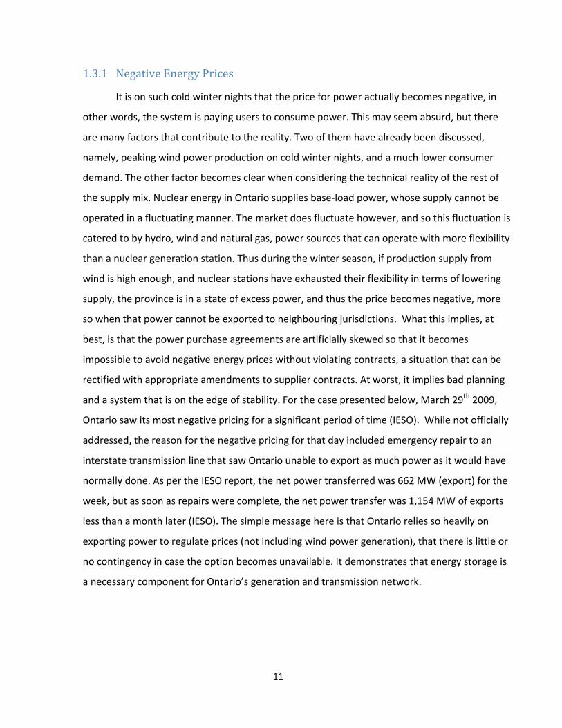
and a system that is on the edge of stability. For the case presented below, March 29th 2009, 

Ontario saw its most negative pricing for a significant period of time (IESO).  While not officially 

addressed, the reason for the negative pricing for that day included emergency repair to an 

interstate transmission line that saw Ontario unable to export as much power as it would have 

normally done. As per the IESO report, the net power transferred was 662 MW (export) for the 

week, but as soon as repairs were complete, the net power transfer was 1,154 MW of exports 

less than a month later (IESO). The simple message here is that Ontario relies so heavily on 

exporting power to regulate prices (not including wind power generation), that there is little or 

no contingency in case the option becomes unavailable. It demonstrates that energy storage is 

a necessary component for Ontario’s generation and transmission network.  

  

12

Hourly Electricity Price - March 29th 2009

-60

-50

-40

-30

-20

-10

0

10

20

12:00:00 AM 12:00:00 PM 12:00:00 AM

Time

Pric

e [$

/MW

h]

 

Figure 1: March 29th, 2009 ‐ Negative Energy Prices in Ontario 

1.3.2  Green Energy Power Purchase Agreements  

The introduction to this work presented the huge discrepancy between the prices paid 

by consumers to consume power and the cost borne by the government to procure that power. 

In the example presented in the introduction the difference was a whole order of magnitude, 

from under 0.08 $/kWh to over 0.8 $/kWh. One might present the case to an Ontarian, that 

power is much cheaper in other industrialized countries, or that given the exploitation of 

nature, the price paid for power in Ontario is too little, and in fact should be much higher. 

These important issues are beyond the scope of this work, but nonetheless, it is important to 

acknowledge that the perception of how much energy is worth is both subtle and subjective. As 

long as people are able to mine power sources at cheaper rates, or ignore the fact that much of 

the energy sustaining the growth and development of modern society today comes from finite 

non‐renewable resources, the perception that power ought to be cheap will not change. Most 

people will acknowledge however, that green power comes at a premium price, usually valued 

as the cost of non‐pollution. In the case of the wind and solar power, the government has 

translated this perception into policy.  As taken from the excerpt earlier, the Green Energy Act 

  

13

states that the policy has been instituted to “assist in the removal of barriers to, and to 

promote opportunities for the use of renewable energy sources”.  

The main method chosen to remove these barriers was instituting green energy power 

purchase agreements that favoured the building and construction of many wind and solar 

generators from a venture capitalist’s or an entrepreneur’s financial point of view. There are 

two main factors that make these power purchase agreements exceedingly lucrative for 

investors and costly for the province.  

1) The Feed‐In‐ Tariff offers higher rates of purchase for power 

2) The Green Energy Act constrains consumers to use renewable energy whenever 

available, due to its intermittent nature. The system controller, the Independent 

Electricity System Operator (IESO) negotiates contracts such that they can leverage 

renewable energy as much as possible.  

This guaranteed purchase‐when‐available policy, as well as higher selling price makes 

renewable energy attractive for investors, but dealing with the uncertainty can be a challenge. 

With respect to wind energy, the  

“IESO centralized wind forecasting, due to begin in the summer of 2010, will help address the variable nature of this energy supply, as it will allow the IESO to understand the periods of time in which they can expect greater levels of wind generation. Equipped with this knowledge, the IESO will be better able to manage all the province’s electricity resources used to meet Ontario’s needs” (IESO).  

1.3.3  The Green Energy Act and Feed‐In Tariff (FIT) 

The Green Energy Act has hence accomplished its policy objective by increasing the 

prominence of renewable energy in Ontario by removing the barriers to speed up its adoption. 

Yet the cost of this progress cannot be gauged since it is too early to do so. The OPA states that 

“the made‐in‐Ontario FIT Program combines lessons learned from Germany, Spain, Denmark 

and other jurisdictions with the unique characteristics of Ontario's electricity system” (Ontario 

Power Authority). The case for Germany is thus presented in this work as well as highlights from 

the case of Denmark. The OPA has tried to emulate other regions where wind power has been 

  

14

significantly adopted and to that end the FIT program represents a good direction. Unlike 

Germany or Denmark however, the transmission and distribution power lines in Ontario are 

aging and where they are not reaching end of life, the switching stations they are connected to 

are. A fact that is recognized as evidenced from the excerpt of the Green Energy Act policy that 

states a goal “to promote access to transmission systems and distribution systems for 

proponents of renewable energy projects.” 

In sharp contrast to this the OPA states that the potential developer  

“…should be aware that, in certain areas of Ontario, it is not currently economically or technically feasible to connect additional generating facilities to the distribution or transmission system. If this applies to your project and you are otherwise eligible to participate in the FIT Program, you may not be able to obtain a FIT contract right away. Your project will be held in reserve until conditions change. 

You (the developer) are strongly advised to investigate options for connecting your project to the grid and to determine whether connection capacity is available before you submit an application” (Ontario Power Authority). 

  It is thus clear that while the transmission connection issue is a significant one, there is 

no strategic plan to measure system performance for either transmission or generation. This 

ad‐hoc nature of transmission connections could have negative repercussions in the future and 

some level of prioritization needs to be planned. While transmission planning does indeed 

influence how and where generation is sited, it is challenging to incorporate it into the policy 

planning process. The formulation presented in chapter 4 of this work, incorporates it as an 

average line‐loss factor per generation type. While the representation of transmission in this 

manner is simple and crude, it can be used to gauge its sensitivity to the costs and benefits of 

optimizing supply mix. Thus even though the consequences of the Green Energy Act include  

investment in transmission and distribution, newly commissioned green energy projects, and a 

commitment to shut down coal production in 2014, the investments may not be strategic in 

nature. The situation for Ontario is that investments into intermittent sources will only increase 

in the short to mid timeframes, that intertie jurisdictional transmission lines are a regulating 

mechanism for Ontario’s internal price of power, that there is no real prioritization for the 

transmission connections being slated within the province, and that since the OPA has stated 

that the Germany and Denmark have been the models on which the various programs for 

  

15

Ontario have been modeled, it is crucial to represent energy storage as a component in 

optimizing supply mix.  

1.3.4  A Beginning for Energy Storage in Ontario 

  Germany and Denmark, the models for the Ontario network, both have significant 

power reserves in terms of energy storage (Lipp, 2007). Replicating their supply mix, or policies 

in Ontario would mean that energy storage would have to play a bigger part, as would a better 

connected electrical network grid. Ontario, in a stage of rapid development with respect to its 

power sector and the usage of renewable energies, must then make a paradigm shift towards 

incorporating energy storage as a fundamental building block of sustainable design. But 

considering energy storage on its own and ignoring other sources of power in the supply mix 

may lead to a skewed vision of the role of energy storage. For example, buying and selling of 

power when needed from an external supplier or jurisdiction may constitute a sort of pseudo‐

energy storage. The opportunity cost of developing and maintaining internal storage may be 

lower or higher compared with purchase agreements that could offer the same level of utility. 

In the case of Ontario, leveraging Quebec’s hydro power to store wind power from Ontario 

during cool winter nights and to sell that power back when needed (perhaps for space heating) 

has been proposed before. But the reality is that external jurisdictions may have their own 

objectives, incompatible with the ones from Ontario. Besides which, if energy storage were 

sited in Ontario, securing the reliability of the grid to effectively transmit that power when 

needed would be higher than the level of confidence associated with importing that power via 

an external grid. Two major requirements are thus identified for Ontario’s energy future; the 

first is to include energy storage and strategic transmission planning and the second is to 

include external power purchase agreements as an integral part of supply mix. In order to 

ascertain the best combination of capacities for energy storage, external market trading values 

and prices must be compared with internal energy storage costs and benefits. The optimization 

of supply mix must account for these factors as well as the environmental impacts of the 

optimized allocation.  

  

16

Ideally, the formulation of the optimization model must also include the secondary 

benefits that the technologies in the supply mix may have. In the case of energy storage, some 

of the benefits include 

‐ Better planning and certainty with respect to power supply, which would allow all 

other power producers on the grid to produce power at peak efficiency, lowering 

greenhouse gas emissions (GHGs) for the same level of utility that would have been 

produced without energy storage. 

‐ Due to the instantaneous nature of most large scale energy storage technologies 

such as pumped hydroelectric storage, battery or flywheel storage, or compressed 

air energy storage, the risk associated with blackouts or brownouts will be 

significantly lowered when energy storage is used, thereby increasing the reliability 

of supply. Quantizing reliability as a simple percentage metric for when good power 

supply quality is maintained does not capture this real decrease in risk. Installing 

energy storage can be considered a sort of insurance policy against catastrophic grid 

failure. 

‐ When storage provides power for peak shaving, the primary environmental benefits 

include off‐setting the greenhouse gas emissions that would have been produced by 

traditional power supply sources to cope with the peaking load, while the secondary 

benefits include a lower price of energy supply that could not have been had 

without storage.  

‐ Other benefits include a more resilient network, characterized by decreased times 

for recovery after a blackout or other local failures and the ability to adapt to 

network outages with multiples paths available to store and transmit power. 

‐ Depending on the storage scheme implemented, a de‐centralized energy storage 

system could have significant advantages over a centralized one. Decentralized 

storage may have reduced initial capital costs, more community stakeholders, make 

for a more resilient network,  and if it made use of existing brown‐field sites such as 

  

17

old mines or hydro ponds, would decrease its environmental footprint further when 

compared to conventional schemes.  

1.4  The New Integrated Power System Plan (IPSP) of 2009 

  With benefits such as these the question of why energy storage has not been 

implemented in Ontario becomes a valid one. The OPA’s initial mandate was one of securing 

supply, and decreasing Ontario’s dependence on coal, thus lowering its environmental impacts 

(OPA). While energy storage can leverage installed infrastructure, it is not a generator of power. 

Much the opposite, in the process of storing and then re‐transmitting power, a conversion loss 

does need to be accounted for. This is included in the optimization model presented in chapter 

four as well. Since the primary objective for the IPSP in 2005 was securing supply, energy 

storage was not deemed necessary until recently.  

However the IPSP in 2008 recognized all of these problems and identified the need for 

more research and a strategic plan of action. This modeling objective of this work is specifically 

targeted towards this new direction. To this end, a model that optimizes power supply mix is 

created.  The optimization model, formulated as a linear program, includes the different types 

of power production technologies, energy storage costs and benefits and energy trading costs 

and benefits. The paradigm shift proposed in the model also includes sustainable design as a 

key element of policy design. The model incorporates the life cycle costing perspective of 

reducing greenhouse gas emissions, specifically Carbon Dioxide (CO2), a potent greenhouse gas. 

A brief introduction to sustainable design is presented in section 1.5 as a precursor to the 

optimization model formulated. While the model concentrates on supply mix, demand side 

management also provides a powerful tool in reducing Ontario’s environmental footprint. 

While the model does not include the demand side of energy use, the constraint for the linear 

program requires production capacity (supply) to meet demand. While future work may vary 

the demand based on demand management methods the constraint of supply meting demand 

would still hold. The new IPSP does include demand side management represented as energy 

conservation. In a letter to the Ontario Energy Board (OEB) dated March 12th 2009, the OPA 

exclusively states the following considerations for the new IPSP: 

  

18

– The amount of diversity of renewable energy sources in the supply mix; 

– The improvement of transmission in northern zones in Ontario and other parts of the 

province that is limiting the development of new renewable energy supply; 

– The potential of existing coal‐fired assets to be converted to biomass; 

– The availability of distributed generation; 

– The potential for pumped storage to contribute to energy supply during peak times; and  

– The viability of accelerating the achievement of stated conservation targets, including a 

review of the deployment and utilization of Smart Meters (Ontario Power Authority). 

1.4.1  An Optimization Model for Supply Mix 

In view of the development of this IPSP and the emphasis on distributed generation, 

pumped storage, as well as better transmission to increase the ratio of renewable energy in 

Ontario’s supply mix, an optimization model is required that incorporates aspects of all these 

goals. It is intended that the framework and model developed in this work be used to 

specifically recommend optimal supply mix, including energy storage capacity for Ontario. The 

main advantages of the model developed are: 

‐ It optimizes the considerations stated based on life cycle & financial consequences;  

‐ The model assumes average/aggregate data as the basis for analysis, but the same 

framework can also be used if better averages or real (singular) project based data is 

input into the model; 

‐ It provides a quantifiable, albeit aggregated methodology to make tradeoffs 

between sustainable design and financial cash flows by including both on the same 

basis of measurement; 

‐ It is able to predict changes to environmental impacts based on changes in supply 

mix; and 

‐ It incorporates an assumed carbon cost sensitivity to supply mix.  If Ontario’s current 

set‐up were thus input as calibration data, it would produce the intrinsic cost of 

carbon associated with Ontario’s supply mix. 

  

19

1.5  Introduction to Sustainability 

  Sustainability as stated by the Brundtland Commission defined the idea as meeting the 

needs of the current generation while preserving the ability of future generations to meet their 

needs. In the crudest sense, preserving the ability of future generation to meet their needs 

implies that all current anthropological activities should not consume any resources that cannot 

be naturally replenished within a generation or two. It could also be inferred from the 

definition that since modern society is able to sustain itself now, as long as we do not degrade 

the planet any further, we will not be robbing future generations of their ability to sustain 

themselves. 

In the context of the optimizing supply mix, sustainability mainly applies to using 

renewable resources, since the non‐renewable ones do not allow future generations to enjoy 

the benefits currently enjoyed by society today. Harvesting resources or any other related 

industrial activity must leave the natural resource in the same (or better) state than when it 

was first exploited. Succinctly, if society uses up or interacts with any biosphere elements such 

as land, water or air for any activity then it must limit or counteract any influences it may have 

that would adversely affect them. One method of accomplishment is to measure these adverse 

effects and then limit, reduce or cease them altogether. An applicable example is to limit CO2 

emissions since it has a high global warming potential as a greenhouse gas (GHG). In order to be 

sustainable however, this measurement must be carried out over the entire life cycle the 

anthropogenic activity, in this case (say) building and operating a power plant.  

Thus a life cycle perspective is helpful because it captures the adverse effects over the 

entire life cycle of an activity, and coupled with the measurement, is expressed as a 

performance indicator of sustainability. Section 3.4.1 applies and explains it for this work.  

  

20

1.6  Chapter Summary 

Though progressive, Ontario has traditionally lacked transparent accounting and 

has spent inefficiently. This has been attributed to a lack of benchmarking and goal 

setting. The current ‘accomplishment’ criterion, the amount of money spent, is justified 

by the government as enhancing public assets, regardless of efficiency. Since tangible 

accomplishment itself is the metric, more expenditure is considered good, whether it is 

over‐budget, strategically executed or otherwise. The regulator’s view of energy storage 

forces the issue of an optimal supply mix. Attributes of the model to optimize supply mix 

are justified in lieu of the new IPSP. It includes: 

‐ Considerations based on life cycle & financial consequences;  

‐ Sustainable  

‐ Prediction of changes in environmental impacts based on changes in supply mix; and 

‐ An assumed carbon cost factored into to supply mix  

  

21

2. Building a Model for Development 

2.0 Chapter Introduction 

‐ This chapter examines the OPA’s model when they recommended the supply mix for 

Ontario in 2005. A critical evaluation is then done based on the assumption stated 

by the OPA. The major note of interest is that the OPA modeled Ontario’s supply mix 

based on countries such as Germany, Spain and Denmark. Thus two case studies, 

with respect to supply mix, policy, transmission, and energy prices are presented, 

the first for Germany and the second for Denmark.  

  

22

2.1  The Case for Ontario’s Power ­ OPA’s model for Supply Mix  

    The Ontario Power Authority released its recommendation for Ontario’s supply mix in 

December of 2005. The basis of their model was a simple one: the first step was to establish 

trends in historical data to create a forward looking forecast of power demand, and then 

compensate for various technological changes as well as incorporate a contingency for load 

growth. They then extrapolated the data for future growth up to 2025. The next step was to 

balance the load growth for base load, intermediate and peaking loads, which more or less 

segregates the type of load so that the resource used to feed the demand, can be closely 

matched to the supply. They grouped the generation by load type (i.e. base, intermediate or 

peaking) and applied a break‐even economic analysis based on the capacity factor (% of time in 

the year that the plant operates at its rated production) to assess the % of time that each type of 

plant should operate to maximize its utility. They then repeated the analysis including a 

contingency factor.  

2.1.1  Environmental Modeling 

  The environmental side of the equation was done using a high‐level life cycle 

methodology. They mention that “the analysis is intended to provide an assessment of the 

relative environmental consequences of different resources and portfolios of resources” (OPA). 

Since the evaluation is not site‐specific, the environmental impacts or not detailed, but rather 

used the gauge the environmental advantage of one technology over another. Each life cycle 

stage, such as resource extraction, processing, transport, construction, operation and 

decommissioning, had environmental consequences. These consequences were grouped into 

categories with a corresponding weighting factor, with a higher weighting factor scoring a 

greater damage to the environment. At the top of the list was greenhouse gases with a 

category weighting factor of twenty (20), contaminant emissions was ten (10), radioactivity, 

land use, water impacts, waste impacts, and resource availability were all weighted equally at a 

factor of one (1).  These criteria and weightings could be deemed as subjective, even simplistic, 

but more accuracy was not required at this initial stage.  The OPA justified its use of the 

weighting thus: 

  

23

“The European Commission has undertaken an exhaustive study, ExternE, on the life cycle impacts of different generating options and has monetized these impacts. Based on the monetized values, implicit weightings of the various impacts can be determined” (OPA).

   To balance the portfolio so that the subjective nature of the analysis was not the only 

factor considered, the ‘scored’ impacts were then coupled together with absolute impacts. The 

absolute impacts were calculated using a life cycle model developed by SENES, the consultants 

commissioned by OPA to do the study. For example, the absolute impacts for a generation 

station would approximate the total amount of Green House Gas (GHG) emissions over its 

lifetime. This index would be tonnes of CO2/MWh of power produced over time for (say) a 

natural gas, coal or combined cycle landfill or digester plant.   

  Several portfolios were then formed by varying the technologies and the percentage 

each of these technologies was used. The portfolio score was then calculated as: 

“Technology A: % of total portfolio (energy) x Total Score for Tech. A = Score A Technology B: % of total portfolio (energy) x Total Score for Tech. B = Score B Technology C: % of total portfolio (energy) x Total Score for Tech. C = Score C ‐‐‐‐‐‐‐‐‐‐‐‐‐‐‐‐‐‐‐‐‐‐‐‐‐‐‐‐‐‐‐‐‐‐‐‐‐‐‐‐‐‐‐‐‐‐‐‐‐‐‐‐‐‐‐‐‐‐‐‐‐‐‐‐‐‐‐‐‐‐‐‐‐‐‐‐‐‐‐‐‐‐‐‐‐‐‐‐‐‐‐‐‐‐‐ Score A + Score B + Score C = Total Environmental Score for Portfolio” (OPA)

2.1.2  Economic Modeling 

  The model was subject to economic drivers by varying the weighted average cost of 

capital (WACC) from 5%, discretely to 8.5% and 11%. They then performed a Levelized Unit 

Energy Cost (LUEC) analysis. As they explain it  

“(LUEC) is a cost measure that allows comparison of options with similar operating regimes. Various options may have different patterns of expenditures, service lives and sizes. One option may be expensive to build but cheap to run compared to another option which is vice versa. LUEC is consistent with, but not a substitute for the more detailed measure, the Present Value Revenue Requirement (PVRR). It is a single number expressed in ¢/kWh or $/MWh, and can be expressed in constant dollars or escalated dollars.  The LUEC methodology levelizes costs by an annuity method which involves allocating costs in equal annual instalments over the operating life of the option in such a way as to give the same cumulative present value as the original expenditures (OPA).”

  

They also varied fuel costs, such as petroleum prices, hydrology for water resources, and 

explored the volatility of natural gas prices. These sensitivities were then used in a model called 

the Portfolio Screening Model (PSM) developed by Navigant Consulting Inc (NCI) that could 

  

24

determine the cost of running the entire power system in the future. The government could run 

the model deterministically or stochastically but would be able to provide cash flows, revenue 

requirements and environmental emissions year by year.   

  The three main aspects of the model, technical, environmental and financial made it a 

robust and effective planning tool given the lack of a precedent model or system expansion 

plan to build from. 

2.1.3  Scenario Planning  

  The OPA moved onto the next stage in terms of modeling the sensitivities to the 

assumed data and this included scenario planning. There were five scenarios in total with two 

different portfolios per scenario being explored. The five scenarios were:  

“∙ Scenario 1 illustrates a future in which all expected procurements, new renewable and conservation resources, and out‐of‐province purchases materialize. ∙ Scenario 2 illustrates a future in which fewer resources materialize, including procurements, new renewable resources, and out‐of province purchases. ∙ Scenario 3 illustrates a future in which the full replacement of a small number of Ontario’s coal‐fired units is unavoidably delayed. ∙ Scenario 4 illustrates a future where demand growth is higher than expected, but where the contribution of conservation and efficiency is also higher. ∙ Scenario 5 illustrates a future which sees a higher success in capturing conservation and efficiency potential (Ontario Power Authority).” 

   

It was somewhat unclear why the OPA chose these particular scenarios for their 

planning purposes. It was stated however that each of the scenarios elicited responses that in 

some fashion pre‐determined what type of supply mix each portfolio should have to meet the 

goals of reliability, efficiency, security and environmental stewardship. Nonetheless, it seemed 

a robust enough model that would accommodate almost all contingencies and was a practical 

way to move forward in short period.  

2.2  OPA’S Model Critique 

  The advice itself seemed sound, rational, well thought out and well executed. But there 

was some level of pre‐determination for each of the model elements. On the technical front, 

there seemed to be a disconnect between the analysis variables, which sought simply to match 

load type with load demand by calculating a break even capacity factor, whereas the final 

  

25

recommendation included neighboring jurisdictions as providing active reliability and power 

purchasing elements.    

  On the environmental front for example, given that the  were weighted 20 times more 

detrimental as opposed to resource availability, waste water or land use, it was not surprising 

to see that nearly 93% of power produced for utilization would come from nuclear and 

renewable sources.  

  On the economic front, there was little information provided (or perhaps it was not 

provided in the public report) on the deterministic and stochastic assumptions that were input 

into NCI’s PSM model. Some of the price volatility graphs were provided but validation of the 

assumed variables was minimal at best.  

  From an objective point of view, the foundation to build a model was lacking, but even if 

an optimization model were built, there was insufficient information to run it. In the light of 

these difficult realizations it is commendable that the OPA was able to achieve a consistent and 

realistic view of future power demand forecasts and system requirements. The IPSP 

compensated for the lack of a strategic plan, the primary objective of which is to adapt to a 

changing landscape and re‐analyze the validity of planned future expenditures for the power 

system.  But even though it is nearly 5 years hence, there seems to be little progress with 

respect to a strategic plan for Ontario’s power future.  

  The more pressing concern is that this advice and recommendation born of a policy 

decision to become an environmental and renewable energy leader is sending an illusionary 

signal of strategy back to policy makers. Not only is there little semblance of a strategic plan, 

save an objective to connect and use as much renewable energy as possible, but the new Green 

Energy and Economy Act may in fact produce undesired consequences for Ontario’s future.  

  Before presenting the proposed strategic development criteria for power system 

development, it becomes important to explore the mistakes of other jurisdictions, where a 

combination of public opinion and public policy has gone awry. One such jurisdiction is 

Germany.  

  

26

2.3  The Case of Germany – Public Policy Gone Awry 

2.3.1  Past Problems  

  Peter Fairley an independent journalist, author and editor summed up the case 

succinctly for the July 2009 edition of the IEEE Spectrum on Energy Policy. In his feature entitled 

‘Germany’s Green‐Energy Gap’ he shows how the country’s power system and policies have 

evolved over time and why.  Germany viewed wind power, and in particular off‐shore wind 

power, as the epitome of renewable energy, much like Ontario.  Germany’s ‘disenchantment’ 

as Fairley puts it, with nuclear power came after the Chernobyl accident in 1986, yet climate 

change and environmental burdens remained as top policy priorities. In an effort to reduce 

GHG emissions the German government passed a Feed–In Law in 1990, in many ways now 

duplicated by other countries, just as it has been recently adapted in Ontario.  

  Ten years later, Germany’s chancellor Gerhard Schroder, passed legislation to shut 

down all of Germany’s nuclear reactors by 2022, partly because the last 10 years stood as an 

attestation to wind power. But environmental policy and energy policy collided after the 

announcement of this legislation. On the one hand, the last 10 years had expended the best on‐

shore wind power sites in Germany so that the only options for wind meant off‐shore turbines. 

On the other hand, environmental lobbyists insisted that off‐shore turbines would severely 

affect migratory birds and other marine life.  In 2005, a resolution arrived from Germany’s 

ministry of the Environment (Bundesministerium für Umwelt, Naturschutz und 

Reaktorsicherheit, or BMU) in the form of designated zones for wind power development. 

Fairley states that while the Netherlands, Sweden and Denmark were installing wind farms in 

water less than 20 metres deep and within 15 km off the shore, the BMU designated zones 

between 20 and 40 metres deep and mostly 40 km off the shore. The old tariff rate of 9.1 euro 

cents/kWh, which was what competition across Germany’s borders were paying, could not 

justify the extra expense and risk that the power producers would have to take. In 2006 

Germany’s new Chancellor Angela Merkel, raised the tariff rate to 0.15 euro/kWh while 

simultaneously making ‘power‐grid operators responsible for running cables to offshore wind 

  

27

farms’. This has rejuvenated the European wind energy producers so that both, on‐shore and 

off‐shore wind installations have been forecasted to increase (Fairley). 

  The lack of a strategic plan in terms policy and consequently financial infeasibility would 

nearly scuttle the fantastic progress that renewable energy had achieved in Germany. In 2003 

for example, the good will of the public had turned to backlash due to the continued policy of 

exorbitant tariffs for wind energy (Fairley). Peter Poppe, then spokesperson for Vattenfall 

Europe, Germany’s third biggest power utility was the quoted as saying “It's certain that the 

burden on consumers has risen because of the economic support for renewable energies…this 

support needs to be reduced. What was originally intended as start‐up finance for the sector 

has turned into a bottomless pit of money” (Furlong, BBC). The significant tariffs that wind 

power had were slowly consuming the German economy.  The lesson for Ontario here is that 

with a price differential for nearly 10 fold form market price for renewable energy with the 

Feed‐in‐Tariffs, it must be careful not to fall into the same trap.  

2.3.2  Grid Stability – Germany vs Ontario   

The push towards renewable energy had only temporarily been averted. With the 

renewed interest in wind energy it became clear that the reliability of the grid may be 

compromised. There were two major factors that kept the grid stable throughout the 

development of wind power, namely energy storage and a high degree of grid 

interconnectivity. Until 2006, Germany’s total electricity production capacity was approximately 

120 million kilowatts (EIA), or about 120  Gigawatts (GW), with approximately 3 GW of pumped 

hydroelectric storage or about 2.5% of total installed capacity (EIA).  Ontario by comparison has 

an installed capacity of about 35 GW (IESO), with only one hydroelectric pumped storage plant 

in operation with a capacity of 174 MW (OPG), which works out to about 0.5% of installed 

capacity. Given the high degree of grid interconnectivity in Europe, Germany could easily 

leverage storage externally, in place like Norway which acts as an added security. Even if there 

were an ‘ideal’ percentage of energy storage, it would certainly be region specific and depend 

on factors such as security of supply, supply mix, external trading contracts and energy policy. 

To give perspective to the role of energy storage being used as a buffer, consider that Ontario 

  

28

was only able to export/import 4600 MW at any given time in 2009 and in that year exported a 

net amount of 10.3 Terawatt‐hours of energy. Averaged out over the year that works out to 

approximately 1175 MW of energy that needed to be exported, mainly because the excess 

energy produced could not be stored. Germany was able to leverage its great expansion of 

wind power because it had significant storage potential. Pumped storage in particular was used 

to manage energy flows, control frequency and provide peak shaving benefits and a provision 

for reserve power, hence increasing the reliability of the grid.  If Ontario is trying to emulate 

other jurisdictions by increasing its share of renewable energy, perhaps it should learn from 

their mistakes. Ontario has only recently started (since late 2009) to see an upsurge in interest 

for pumped hydroelectric storage.  Like Germany, Ontario will need to look at leveraging 

renewable infrastructure through energy storage. The question to be answered is how much 

energy storage would be optimal for an expanding Ontario, and more importantly how can this 

development be executed in a strategic manner?   

  To achieve a similar level of utility as energy storage might provide, Ontario might 

consider developing transmission capabilities so that it can export all of its excess its power to 

neighboring jurisdictions and then buy it back as and when required. Ontario already trades 

power with Manitoba, Quebec, New York, Michigan and Minnesota (IESO), and could 

potentially set up better bi‐lateral power purchase agreements with all of them. Quebec in 

particular might be considerably strategic since its power mix contains over 95% of installed 

hydro‐electric power – with sufficient storage potential and boasts much lower carbon 

emissions. Nonetheless, internal energy storage would serve as a better strategic investment 

given its current virtual non‐existence. Other market players such as New York that trade with 

Quebec may offer better incentives than Ontario can afford. Unpacking these market interests 

is fraught with difficulties because of the public‐private tensions that arise. Consider that the 

bulk electrical transmission systems are state owned but that the these entities while trading 

power with each other need to co‐ordinate the private sector as well. With the advent of 

renewable energy in Ontario bringing in new private entities, as well as older nuclear entities 

such as Bruce Power vying for market share, modeling the situation can be quite challenging. 

The political will has as much to do with keeping the grid stable as do power lines and other 

  

29

electronic control equipment. Recognizing and learning from how policy can produce 

unintended consequences can help to get a better perspective on how to institute effective 

policy in Ontario. 

2.3.3  German Legislation – Policy Constraining Practicality  

Germany is a leader in the energy policy and renewable energy arena, but there are 

crucial lessons to be learned from their policy errors. Germany’s energy policy has in fact 

evolved considerably in the last decade. The ban on nuclear power plants stemming from the 

successful implementation of renewable energy seemed to be a step in the right direction. Yet 

the policy seemed mistimed and drastic indeed. The pressure to keep nuclear plants open 

longer has become a contentions policy issue. The two major factors why nuclear power is back 

on the agenda are security and availability of supply, and increasing electricity prices (Duffield, 

2009).  Other factors against the nuclear option the safety concern that the power plants will 

need to be operated past their design lives and that new safety factors would need to 

implemented, cost overruns, although these have more so been associated with brand new 

stations, and that economically importing power made better economic sense. Yet in February 

of 2010 Bloomberg Business Week quoted Guido Westerwelle, vice chancellor and head of 

Angela Merkel’s Free Democratic Party, her coalition partner, and Germany’s Foreign Minister 

as recently stating that abandoning nuclear power would be a serious mistake. (Czuczka, 2009) 

What has happened in Germany is that policies with competing priorities have 

segregated and polarized public and political opinion. Security of supply dictates that natural 

gas and oil imports from Russia, Algeria and possibly Iran must decrease, and nuclear power or 

coal should take its place. Yet environmental considerations negate both coal and nuclear for 

different reasons, coal because carbon capture technology cannot yet eliminate GHG emissions, 

and nuclear because other renewable energies such as wind should be able to fill the gap that a 

nuclear phase out would leave. Yet the story is still not complete, safety concerns would 

advocate a phase out of nuclear power, yet economic factors such as rising electricity prices 

indicate that the investment in safety may be warranted to stabilize energy prices. Coal is fast 

becoming the fuel of choice to quell many of the issues, yet it comes bundled with enormous 

  

30

environmental effects that make an interesting trade‐off. Ontario needs to learn from the 

evolution of these policies so that a similar fragmented situation can be avoided. It is essential 

to recognize that there must inherently be trade‐offs when instituting policy and only when 

they are recognized can an informed decision be made, with predictable results.  

 In fact, coal in Germany has bizarrely become a requisite to phase out nuclear power. 

Michael Pahle of the Potsdam Institute for Climate Impact Research states that …  “the BMU 

also published an energy policy roadmap in early 2009 which targets 40% of all electricity in 

2020 shall be generated by highly efficient coal power plants. It explicitly refers to this measure 

as a necessary condition for the prioritized nuclear phase out” (Pahle, 2010). 

He also states that… “The broad support along the administrative spectrum reflects only the current political constellation and considerable uncertainty remains. On one side, the nuclear phase out is continuously challenged by the liberal and the conservative party, and lifetime extensions for current plants will likely become reality. On the other side, the Green party fiercely opposes new coal power plants, even though the new plant in Moorburg has shown that in coalitions concessions must be made. In fact, of all factors influencing technology choice neither seems so much out of the investor’s control as prolonged political support. Correspondingly, the appeal for stable investment frameworks is echoed all around. If however – as present trends seem to indicate – coal will become established as a cornerstone in German energy policy, then political support will very likely sustain into the future” (Pahle, 2010). 

Political stability is an important ingredient towards a unanimous consensus and 

strategic plan of action. It is imperative for such considerations to be taken into account at a 

high level of planning. While this case study demonstrates that policy implications, such as the 

ones produced from the Green Energy and Economy Act may be intended as progressive tools, 

it is important to envision scenarios where the policy may backfire, and how changes in political 

will might affect the future of products borne from them in the present.  

The final case under study is presented for Denmark. The OPA has stated that certain 

policies need to be revamped and technologies need to be looked into via the new IPSP. The FIT 

program however, based on the one implemented in Germany, may have similar repercussions 

of raised electricity prices and increasing public debt that’s owed to private investors.  Yet 

political savvy cannot change the reality of power production. Even though nuclear energy is set 

to be phased out in favour of coal, the environmental impacts are worse than if the legislated 

  

31

phase out was not passed. Bode (2009) discusses the effects of the nuclear phase out using 

direct and indirect effects. He states that  

“while the direct effect describes an increase of electricity prices due to the replacement of power plants bearing higher marginal costs than the previous one, the indirect effect is characterised by a potential increase in CO2 emissions due to the substitution of nuclear power plants through the ones that use fossil fuels. Potential additional emissions lead to higher CO2 prices and hence (among other factors) to a higher electricity price” (Bode, 2009). 

He concludes that, “consequently, an increase in emissions and thus in carbon and 

power prices can be expected if the phase‐out is not revised. If renewable energy is to replace 

the reduced capacity of the nuclear power plants shut down, additional support mechanisms 

would be necessary” (Bode, 2009). 

The decline of nuclear energy in Germany affects prices outside of Germany as well, 

including Finland and Denmark. The latter was also used by the OPA as a model for Ontario, and 

there are some key lessons for Ontario from exploring the execution of energy policy there.     

2.4  The Case for Denmark 

  Denmark is an excellent role model for Ontario since it successfully implemented 

renewable energy through a healthy mix of policy and public interest. Lipp iterates that  

“with no (known) indigenous fossil‐fuel resources, and an early decision (resulting from steady public pressure) not to build nuclear power plants, the Danes’ options for self‐sufficiency were limited…It is one of the few countries in the world that actively, and in a sustained way, supported RE development from the late 1970s, through the 1980s and 1990s to the present. Where other countries’ programmes waxed and waned, the Danes were persistent in pushing this sector. Energy security, self‐sufficiency and efficiency have remained the principal objectives of energy policy throughout this time” (Lipp, 2007) 

2.4.1  Denmark’s Strategy   

Simply investing in renewable energies was an insufficient strategy.   

“Public ownership was directly encouraged through a generous tax allowance (for own generation) and later complemented by a FIT. The FIT compensated developers for the environmental attributes of the power, thereby making it possible for the investments to be profitable. The local ownership helped create widespread support for RE, especially wind, because benefits were distributed across a wide group of people…Central to the diffusion of wind energy in Denmark was the FIT…It obligated utilities to purchase wind‐generated electricity at a rate that equalled 85% of the price paid by consumers. Introduced in 1993, the FIT was the stimulus needed for widespread wind development and allowed projects to move beyond wind 

  

32

enthusiasts to a bigger share of the population…Other policies complemented the FIT, including a direct subsidy and tax exemption to private turbine owners, a 30% investment subsidy and tax‐free electricity generation up to 7000 kWh”(Lipp, 2007).  

Significant policy incentives were offered that made the market come alive. The policy 

implications and incentives were couples with something else – transmission capacity.  

Jacobsen (2010) reveals that  

“the prevalence of wind power in Denmark is the highest in the Nordic power system. There were 5104 wind turbines with a total installed capacity of 3169 MW in January 2009 in Denmark. In 2007, wind power production comprised 7173 GWh, or 21.8 percent, of the electricity consumption in the country. It is expected that wind power will account for 25 percent of total consumption in 2010.”  

More importantly however he also states that  

“the country’s electricity system has strong external connections via transmission lines to Germany, Sweden and Norway. Electricity networks in Western and Eastern Denmark are not yet connected, and Western Denmark retains almost 77 percent of the total Danish wind power capacity. In January 2007 electricity production by wind turbines comprised approximately 44 percent of Western Denmark’s electricity consumption and approximately 36 percent of the total consumption of Denmark” (Jacobsen, 2010) 

2.4.2  Policy Consequences   

The two important factors for renewable energy development in Denmark are 

sustainable political will and implemented policy, and an excellent transmission system. Policy 

incentives are exceedingly important to consider for two reasons: 

‐ They artificially affect the amount of investment in renewable energies 

‐ They may have unintended consequences 

The first of these concerns is somewhat understandable, but not altogether predictable. 

Lipp demonstrates that when 

“explicit support for wind energy changed in 2001. Under a new government, there has been a shift away from direct support for RE to a free‐market (neo‐liberal) approach in the energy sector in Denmark. The FIT was modified in 2001 and wind generators are now paid the market price, set by the Nordic Power Exchange, and an environmental premium of 0.10 DDK/kWh (approx. 0.013 €/kWh). This premium is felt to be too low to continue growth in this sector” (Lipp, 2009). 

The effects of this new shift in policy was realized by the slackening pace of new wind 

turbine installations across Denmark. While this consequence could have been expected, albeit 

  

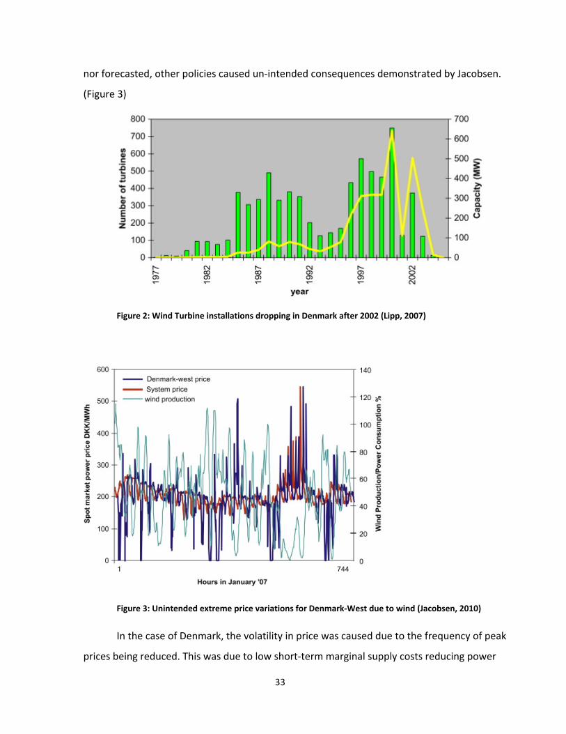
33

nor forecasted, other policies caused un‐intended consequences demonstrated by Jacobsen. 

(Figure 3) 

Figure 2: Wind Turbine installations dropping in Denmark after 2002 (Lipp, 2007) 

 

 

Figure 3: Unintended extreme price variations for Denmark‐West due to wind (Jacobsen, 2010) 

  In the case of Denmark, the volatility in price was caused due to the frequency of peak 

prices being reduced. This was due to low short‐term marginal supply costs reducing power 

  

34

prices and because subsidies for renewable energy technologies were much better outside of 

Denmark (trading jurisdictions) than inside (internal ones). Additionally, total generation 

capacity in the area increased so naturally importing power became cheaper (Jacobsen, 2010). 

  One of the main problems for Demark is that it relies too heavily on external power 

production to regulate its internal market. While the installed wind capacity is staggering, there 

is little storage capacity, a fact Jacobsen says needs to be addressed, and that the price 

differential between selling and buying power may not be advantageous of the country. If 

Ontario is learn from Denmark the takeaway message is that: 

‐ With greater external transmission connections and internal ratios of renewable 

energy, external markets can dictate internal price fluctuations; 

‐ Policies such as FIT are only successful as long term tools, political will and policy 

needs to compliment the nature of the program so as to reduce any unintended 

consequences; and 

‐ Energy Storage is an essential key component when increasing renewable share in 

the supply mix. 

It is with the lessons learned from both case studies and the new IPSP from the OPA that 

the linear programming model to optimize supply mix is developed. 

 

  

35

2.5 Chapter Summary 

The OPA’s model for supply mix was not strategic due to the predetermination of 

renewable power and lopsided weightings when evaluating sustainability. Additionally, no 

trade‐offs between sensitivity were reported.  The cases for Germany and Denmark were 

presented since they were used as models by the OPA. The lessons learned are summarized. 

Table 1: Lesson for Ontario from Germany and Denmark 

Issue  Case of Germany  Case of Denmark  Lesson for Ontario

Energy Storage  Lots of Energy storage  

~ 3GW  ‐ Can leverage renewable 

Leverages storage externally in a competitive 

market 

Cannot leverage renewable, external market not very 

competitive – Consider Storage  

FIT Program Model  Initially Successful – Turned into ‘money pit’ – 

low public support  

Initially Successful – rates too high‐ then reduced – decline in renewable energy sector for new 

wind installation 

Re‐evaluate long term FIT contracts. Re‐evaluate FIT pricing. Re‐evaluate will‐purchase‐if‐produced 

policy 

Pricing Problems  Off‐shore incentives for wind pricing too low – Environmental laws relatively stringent compared with 

neighbours. Temporarily stagnated investment.  

Incentives were eventually increased. 

Inefficient internal pricing mechanism – Result was externally selling low and buying high of power internally produced. Wildly fluctuating and some negative pricing. 

External purchase and selling agreements and 

internal pricing mechanisms need to be 

aligned  

Policy Problems  Fragmented Policy and polarized public regarding nuclear phase out policy. Legislation may possibly be reversed. Off‐shore 

wind  

  The Green energy Act is not strategic – Unintended 

consequences of implemented legislation 

Transmission Capabilities  High level of interconnection – transmission and 

distribution 

Very high level of interconnection – transmission and 

distribution 

Relatively low level of interconnections – need for strategic investment between transmission, 

distribution and procurement 

  

36

3. Paradigm shift 

  3.0   Chapter Introduction 

The chapter builds from the lessons learned and recommends factors to consider while building 

the model of supply mix optimization. They include sustainability, resource availability and 

transmission issues, system antics and risk mitigation, financial and economic considerations, 

trading power externally and most importantly energy storage. Justification for using the linear 

model approach is presented. The objective of the model is to optimize supply mix for Ontario, 

including sustainability life cycle considerations, energy storage and energy trade, to evaluate 

the tradeoffs between the various factors. These factors had not been modeled as tradeoffs by 

the OPA, and so generating the logical mechanism to do so was of primary concern.  

  

37

3.1  Benchmarking Goals 

The model used by Ontario for developing the power sector is reactive to public 

pressure, government mandates and environmental lobbyists rather than being proactive and 

instituting changes that would allow some measure of control and predictability in terms of 

energy use.  There are several reasons why this is the case; 

‐ Government direction, political will and strategy may change with party changes; 

‐ In addition to be being vague, the Green Energy Act Legislation does not clearly define 

the beneficiaries of the policy itself. That the objective of a ‘greener’ Ontario is to be 

achieved by using tax‐payer monies for welfare development is clear – but should this 

be achieved by subsidizing private investors? Or by investing in public owned utilities? 

Are the public of Ontario the beneficiaries of the policy or is it private investors? The 

opportunity cost for investment is vague, hence the strategy is ill‐defined and thus it 

becomes possible that the Green Energy Act may debt the public it is supposed to serve. 

‐ Even if the Green Energy Act were to define the favoured beneficiaries of the policy, the 

objective towards sustainable energy use is vague – there are no benchmarks in terms 

of measurable indexes. (E.g. atmospheric CO2 levels, water‐way contamination levels, 

energy intensity usage, energy use/capita/year) etc. This means that ‘progress’ is not 

measurable with respect to a frame of reference. 

‐ The IPSP, the product of the initial mandate to the OPA to develop Ontario’s energy, is 

revisited on the basis of the initial supply mix. While this means that changes to the plan 

can only be made within a certain threshold of the initial supply mix advice, there has 

been no effort towards bettering the initial model of sustainable practice. The OPA’s 

initial plan was a good one, given that there was no starting point and the paradigm of 

practicality was the strategic way forward.  That is no longer the case, yet there has 

been little focus on strategic development. 

Other challenges the OPA had to cope with included economic constraints, time 

constraints and challenging population growth factors such as population immigration and 

  

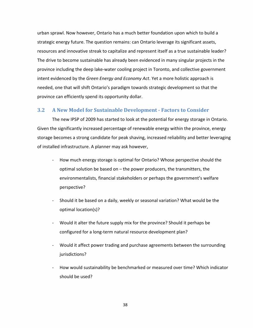
38

urban sprawl. Now however, Ontario has a much better foundation upon which to build a 

strategic energy future. The question remains: can Ontario leverage its significant assets, 

resources and innovative streak to capitalize and represent itself as a true sustainable leader? 

The drive to become sustainable has already been evidenced in many singular projects in the 

province including the deep lake‐water cooling project in Toronto, and collective government 

intent evidenced by the Green Energy and Economy Act. Yet a more holistic approach is 

needed, one that will shift Ontario’s paradigm towards strategic development so that the 

province can efficiently spend its opportunity dollar. 

3.2  A New Model for Sustainable Development ­ Factors to Consider 

  The new IPSP of 2009 has started to look at the potential for energy storage in Ontario. 

Given the significantly increased percentage of renewable energy within the province, energy 

storage becomes a strong candidate for peak shaving, increased reliability and better leveraging 

of installed infrastructure. A planner may ask however,  

‐ How much energy storage is optimal for Ontario? Whose perspective should the 

optimal solution be based on – the power producers, the transmitters, the 

environmentalists, financial stakeholders or perhaps the government’s welfare 

perspective? 

‐ Should it be based on a daily, weekly or seasonal variation? What would be the 

optimal location(s)?  

‐ Would it alter the future supply mix for the province? Should it perhaps be 

configured for a long‐term natural resource development plan? 

‐ Would it affect power trading and purchase agreements between the surrounding 

jurisdictions?  

‐ How would sustainability be benchmarked or measured over time? Which indicator 

should be used? 

  

39

‐ Should the optimal solution be based on system wide generation or simply by 

generation type? What would be the tradeoffs between either? 

Such a comprehensive view is challenging to formalize, thus the best way forward is to 

list all the factors that a planning body might consider, and validate or justify the assumptions 

further made.  

The primary goal of this exercise is to produce a model that would yield an ideal natural‐

resource/sustainability based development policy for electricity production in Ontario. The 

method to achieve this goal is to relate the different factors involved, formulate an objective 

that would optimize power supply mix, include energy storage as part of the formulation, justify 

any assumptions made, solve the problem using a technique that is efficient to yield better 

results than the model that has already been used. The sensitivities and tradeoffs then need to 

be evaluated in a logical manner so as to propose a strategic policy decision.   

As was iterated earlier, the main factor for a non strategic plan of action was a lack of 

benchmarks. Most countries that participated in the Kyoto agreement set their environmental 

benchmark with respect to greenhouse gases at 1990 levels (Laurent, 2003). Whether this was 

an appropriate benchmark for all the participants is out of scope for this work, but suffice it to 

say, a benchmark is a first step towards performance improvement.  

For Ontario, appropriate benchmarks could be kgCO2/kWh of energy produced or 

consumed, intensity such as kWh/km2/year, energy use/capita/year or energy use/$ GDP or 

even a simple metric such as total electricity use/sector/year. Benchmarks help to trend 

improvement over time and thus answer the question if a particular investment strategy is 

performing as predicted. In the case where results are as good as or better than can be 

expected, identification of the investment components that most contribute towards success 

ought to be enhanced. In the case where the performance is poor, the strategy may need to be 

tweaked. The time‐based measurement of an investment lends itself well to the idea of a 

product life‐cycle. So long as the predicted expectation of the investment is not under or over‐

achieving, a symptom that might suggest a fundamental re‐evaluation of the assumptions or 

theory, a life cycle approach yields a good indication if the investment is worth it. 

  

40

3.2.1  Sustainability  

One of the mainstream tools to evaluate such an investment for sustainable design is a 

Life‐Cycle‐Analysis (LCA). The investment for example, in the building of a nuclear station does 

not simply have to pay off in terms of financial and economic terms; it has to make sense 

environmentally and must also break‐even (in a reasonable time frame) from an energy point of 

view. The tremendous amount of energy that goes into the manufacturing of the various 

components, the transportation and construction of the facility and the mining of the fuel, 

operation and maintenance must at some point in the future, before it is decommissioned, be 

balanced with the net amount of energy that the facility produces. An analysis with this kind of 

perspective, based on the life‐cycle of the plant, can be termed an LCA. The new model for 

optimal power supply‐mix must incorporate an LCA approach on the environmental front that is 

more comprehensive than the weighting criteria described early on in Chapter 2.   

3.2.2  Resource Availability and Transmission Issues 

A model for optimizing power mix cannot really be evaluated without knowing the initial 

state of the resource available for development. This is a significant problem because not only 

do the resources have to be developed where they exist in the physical world, but they energy 

has to be transported, either through fuel shipping or transmission lines to where the power 

supply is needed. A prime example to illustrate the point is off‐shore wind development. While 

the resource availability excellent, the environmental and economic cost of transmitting power 

over or under the water may not be worth it when compared with conventional generation 

such as coal, unless it were subsidized in some way.  

The resource availability problem is complex, and to borrow a common a euphemism is 

a ‘chicken or egg’ problem. In order to develop a transmission network one needs to know 

exactly where the generation station is going to be located, but the strategy for developing a 

natural resource is directly tied to how much the transmission of that power may cost. Note 

that the environmental costs in developing the resources will be considered as part of the LCA 

approach. These problems are intertwined and need to be considered more carefully so as to 

yield a strategic policy.  

  

41

The model must thus incorporate some measure of the cost of resource availability with 

respect to power transmission before being optimized. 

3.2.3  System Antics and Risk Mitigation 

Consider the risk of a blackout. What cost might one pay to avoid or mitigate the risk?  

Perhaps the power supply mix is best optimized from a risk mitigation perspective. Certainly 

some aspects of securing an energy supply have to do with political, geographical and socio‐

economic risk mitigation. The choice to develop an internal coal resource in Germany for 

example rather than depend on gas or oil imports is a form of risk mitigation.  But some 

resources types are inherently risky as well. Resources such as hydro power naturally lends 

itself to be more resilient and less risky when it comes to preventing blackouts, mainly because 

it can ramp up power production in a matter of seconds thus helping to regulate the voltage 

across a network. 

 Including energy storage in the form of pumped hydroelectric power has this secondary 

advantage we well. Coal or nuclear power for example take much longer to adapt to changes in 

a transmission network but represent a more long‐term, predictable and stable source of 

power, as opposed to hydro electricity. But there are other criteria that can be quantified using 

technical metrics for which the system could be optimized. Examples of such metrics include 

reliability and resiliency of the network itself. If the perspective for optimization placed a higher 

priority on risk management or power supply investors and developers were significantly risk 

averse then the objective function might be tweaked to weigh these characteristics 

prominently. The resulting policy decision arising from the optimization may be vastly different, 

if for example the objective space only included financial considerations.  

Ideally, the model must also recognize and incorporate this measure of risk and 

reliability, although at the outset, this may seem significantly challenging when optimizing 

power supply mix for a diverse network.   

  

42

3.2.4  Finance and Economics 

The most traditional way of looking at an optimization of investments are the relative 

indicators of costs and benefits based on an assumed or identified level of risk. The distinction 

here is that the financial point of view may be based on a single project or consist of a portfolio 

or projects. For Ontario, a financial optimization may yield a supply mix that heavily favours 

coal or nuclear energy. Resources that are plentiful, tend to be less volatile in terms of fuel 

costs so long as future purchase agreements can be made and consequently have been the best 

value in terms of investment return. An economic perspective might look at optimizing a power 

supply mix portfolio that was welfare based, capturing job creation and wealth distribution as 

benefits to offset capital costs. Coupled to these factors are variables such as interest or 

borrowing rates and required rates of return. A policy decision based on such a perspective may 

be artificially influenced by other policies such as carbon taxation. Environmental externalities 

may be internalized by providing subsidies to renewable resources while instituting resource 

type based taxes on revenue from non‐renewable ones. A good example presented earlier were 

the subsidies of power purchase agreements for the FIT program outlined by the OPA. An 

optimization for supply mix based solely on environmental criteria as opposed to economic 

ones would yield a different policy of preferred natural resources to be developed. Both are 

important nonetheless and serve as a basis for evaluating tradeoffs between strategies.  

Financial costs do provide a ready basis for comparing all forms of value, even if the 

individual is unaware of the value they inherently accept or assign. For example, the cost of 

gasoline is a ready‐made indicator of the cost of carbon, and in consuming it, people 

automatically value its embedded economic and environmental effects as acceptable. Because 

of this inherent quality of money as in indicator of value, the optimization model proposed will 

be one based on costs and benefits, but will try to incorporate other factors on the same 

common denominator, that is, the dollar($). In most cases for the power industry, the 

development of a project depends on the cost of construction, operation and maintenance cash 

flows, expected revenue, which may be probabilistic or deterministic in nature and any interest 

rates, which in most cases is external to the investment itself.  

  

43

The model must incorporate financial and economic considerations into the analysis. The 

assumed factors such as interest rate should be rigorously examined through a sensitivity 

analysis as should any other variable assumptions. The OPA in fact did conduct such an analysis, 

with rates ranging from 8% and higher.  While the selection of these rates is considered to be at 

the higher end of the spectrum given the recent global financial crises at the time if this writing, 

they were deemed acceptable rates of growth in 2005.  

3.2.5  Trading Power and Purchase Agreements 

  One of the most important and practical factors under consideration with respect to 

optimizing power supply mix is the selling and buying of power from neighbouring jurisdictions. 

This is important because it factors into the policy decision regarding development of certain 

types of natural resources. Much like the economic and manufacturing sector across borders, if 

it is cheaper to simply import power and consume it, rather than developing a local production 

supply, then perhaps the policy will be geared towards securing better power purchase 

agreements with surrounding power suppliers. This may conflict with other types of policy, such 

as independent of energy supply and security, as well as risk that may dictate an internal power 

supply that is guaranteed, the reliability of which does not depend on external factors. 

Importing and exporting power comes with its own sets of challenges, and is geared toward 

rigorously measuring the total amount of power being imported or exported, so that costs can 

be precisely credited and tracked. These regulated external power purchase are limited by 

transmission capacities and may differ from the internal standard of power trading. 

Competition, even on the this level is evident by the fact that the Province of Quebec, which 

borders Ontario, but is also able to sell power to the New York Power Authority (NYPA), will in 

fact sell their power to the highest bidder. 

  Associated with external purchasing of power is also an embedded environmental cost. 

Importing cheaper power externalizes these costs and impacts, thus the price of purchase may 

not include the real environmental impact. This cost should at the very least be evaluated and 

included in a sustainability based policy for supply mix.  

  

44

The model must allow for import and export of power. It must however try to 

incorporate the environmental externalities of importing power, in addition to the financial 

ones. An unconstrained objective from this perspective may require external influences to be 

constrained; nonetheless the tradeoffs between local and foreign power purchases and 

consumption will need to be evaluated using a sensitivity analysis. 

3.2.6  Timing is Everything – Energy Storage 

The price of power is usually dictated by market supply and demand in much the same 

way any other economic good is influenced by supply and demand. The main difference 

between products and energy is that the price volatility is much greater in the power sector and 

significant adjustments in market price may take place in the span a few minutes to few 

seconds depending on the type of market and jurisdiction. In the case of Ontario, the price for 

electricity can even dip into the negatives. The internal Ontario market is fairly competitive but 

for the most part the Independent Electricity System Operator (IESO) is able to predict with a 

good degree of certainty the amount of power required in the day‐ahead market and is able to 

secure contracts within the legislative and power purchase agreements that have been signed 

by the various market participants.  

As demand goes up during the day, so is there a corresponding increase in price. At 

night when demand is fairly low the price drops significantly. Energy storage would work by 

buying power at this lower price and ‘storing’ it until it could be used later on when demand is 

higher. The efficiency losses due to conversion are made up for sufficiently in the price 

differential. Power may not be sold if that difference is not large enough. The same principle 

can be applied when power is bought or sold to other jurisdictions. If Ontario were selling 

power, it would indicate a surplus with a relatively low selling price. As in the case with 

Denmark, wind power produced internally must be used or sold since Denmark has little in the 

way of storage (albeit a higher relative percentage than Ontario), the excess is sold to Germany 

or other jurisdictions that can either store or use it at that time (Bode, 2009). 

Generally, when Ontario needs to buy power from another jurisdiction, say Quebec or 

New York, the price of import for Ontario will be relatively higher than the price of export. Since 

  

45

Ontario has minimal energy storage, importing power would be indicative of a non‐productive, 

costly, or insufficient internal supply market. As mentioned, according to the IESO supply 

overview Ontario sold a net amount of 10.3 TWh to its surrounding jurisdictions. If the province 

is mandated to use subsidized green energy while additionally paying a premium for it, but then 

has to sell that energy (in all likelihood at a lower price) because the demand at the time of 

generation is relatively lower, it does not provide an advantage for Ontario but in fact may 

serve to subsidize power usage in other jurisdictions. A similar situation has been occurring in 

Denmark where power is exported at a lower price, bought back at a higher price, and the 

Danish investments in wind and transmission are in fact benefitting external jurisdictions as 

well (Bode, 2009). In the case of Denmark however, a highly interconnected transmission 

network does given them a semblance of choice for energy trade, with external competition 

resulting in a somewhat narrower price differential. Time of use for electricity is thus critical in 

determining its price and utility in the internal and external markets.  

Thus, the model must allow for time dependent analysis. Timeframes should account for 

daily and seasonal cycles, to effect an optimal policy decision with respect to present 

requirements, but the timeframe must also be extended to a much longer horizon so that it may 

be used a planning tool for future deployments. 

 3.3  Model Construction  

The major factors that an optimization model must thus include are: environmental 

sustainability, resource availability from a geographic point of view, potential transmission 

developments, system resilience, risk and reliability, from a technical and financial perspective, 

economic efficiency, an analysis based on time and price (supply and demand), energy storage, 

and relationships including the import and export of power. Drawing out and identifying these 

various factors has yielded a complex picture. Most optimization models are not 

comprehensive enough to deal with all these variables simultaneously and so they may de‐

construct the problem down into more manageable chucks and optimize them separately.  

Dealing with all these various facets simultaneously will allow the significant advantage 

of being able to quantify the tradeoffs between them, as opposed to optimizing each 

  

46

component separately. For example, one might ask the question, at what price differential does 

it make better economic sense to build more energy storage as opposed to externalizing the 

utility by buying and selling power? What interest rate of borrowing money to construct 

electricity production facilities makes it more practical to simply buy the power from other 

jurisdictions to meet internal demand? How best to quantify the tradeoffs between the 

alternative of building a nuclear station closer to an urban centre as opposed to constructing 

off‐shore wind turbines?  

Given these criteria, variables and perspectives, the problem of optimizing supply mix 

with the goal of determining strategic policy does seem challenging. The primary driver to 

attempt such a exercise has already been illustrated, that a policy decision is by nature 

intended as a trade‐off, but recognizing, quantifying and evaluating those trade‐offs are 

certainly as paramount as the decision itself. The secondary driver is the calibration and 

effective utilization of the model as a benchmarking and policy planning tool.  

3.3.1  The Linear Programming Model ‐ Justification 

It might seem at the outset that using a linear programming model for such a complex 

set of variables is too simplistic. There are several reasons why such a model must first be 

employed: 

‐ Building a linear model has helped in identifying the high‐level factors that would 

play a part in determining optimal supply mix. A much more detailed model would 

have required scrutiny of every high‐level factor identified here with a 

corresponding slew of variables that may have rendered the formulation convoluted 

and bogged down with too many intricate details. 

‐ Construction of a linear model would allow for a first stab at the problem and allow 

a solution, (which may not be as optimal as if it were computed using more 

advanced methods) that would yield a general indicator and an intuitive 

understanding of the relative importance of all the variables. It is accepted that 

certain characteristics, such as wind load distribution, peak shaving prices or 

  

47

capacity‐based extrapolated construction or maintenance costs are not linear in 

nature.  

‐ A linear program has various characteristics such as duals, and sensitivities that 

would make it useful in identifying how certain factors affect others, thus identifying 

tradeoffs. In fact the model constructed will be in the form of a linear programming 

minimization problem – the dual of which could se stated as a primal linear 

programming maximization if required. The simplicity of a linear model would allow 

it to be easily run as a preliminary simulation tool. 

‐ Models primarily designed for predictive or planning purposes may get significantly 

complex without yielding a corresponding increase in accuracy. A simpler model, 

while less accurate is sometimes the best way to understand the nature of the 

problem. It can then be tweaked or reformulated with more realistic components so 

to yield a higher accuracy if required. 

3.4  Model Assumptions 

Acknowledging that the increase in complexity of a model may not necessarily result in 

a corresponding increase in its accuracy, certain assumptions need to be made in order to build 

the objective function for the optimal supply mix problem.  

3.4.1  Sustainability Assumptions 

The OPA when recommending their model for supply mix advice, considered the LUEC 

as their basis of comparison. In terms of sustainability, the basis for all comparisons of 

alternatives is accomplished by choosing a functional unit. (Finnvenden, 2009) et al describe the 

functional unit as “a quantitative measure of the functions that the goods (or service) provide”. 

In the case for power generation, a functional unit of quantity/Megawatt hour (MWh) can be 

chosen.  

To incorporate sustainability criteria in their model, the OPA weighted the options 

based on their impacts on the environment, with greenhouse gas emissions given the highest 

weighting of 20. This approach while rudimentary was effective in capturing the operational 

  

48

stage of emissions from any type of power generation facility. It cannot however represent the 

embedded energies in the manufacturing of the components of the facility, the environmental 

impacts of construction or transportation or cannot be used as a trade‐off for other benefits. 

Capturing these effects is challenging because the boundary for the life cycle study must be 

clearly defined. In other words, how far back in the supply chain should the effects of 

construction and transportation be accounted for? For the purposes of the linear optimization 

model, a full fledged life cycle analysis or assessment would be laboriously long and would not 

cater to the main objective of recommending an optimal supply mix. Neither would it provide 

an easier way to evaluate tradeoffs between the environmental and financial goals of the 

power sector.  

The economic input‐output model for life cycle assessments for Canada, was developed 

with collaboration between Carnegie Mellon University and the University of Toronto, and is 

able to provide a linear estimation of the life cycle impacts of power generation related 

activities.  The Economic Input Output ‐ Life Cycle Assessment (EIO‐LCA) model will be used to 

represent the environmental impacts based on generation type (Carnegie Mellon). It covers 105 

sectors from the Canadian economy and requires the producer price for an activity (say power 

construction) in 2002$ as requisite input. Based on the economic input, it disaggregates the 

production price (and assuming the same level of utility) over all the 105 sectors in terms of 

economic value, and is thus able to estimate the level of work associated with the other sectors 

in the economy (Carnegie Mellon). From this set of distributed economic values, it uses an 

averaged proportionality coefficient to produce the associated level of energy use, CO2 

emissions, water contaminants and electricity use per sector.  

The optimization model proposed here will input the averaged value of economic 

activity per generation type (note that this could also be done on a per project basis), into the 

EIO‐LCA, and it assumed that the model is run for CO2 emissions only. The total value of the CO2 

emissions over all the Canadian sectors will then be multiplied by a carbon cost or carbon tax to 

bring it in line with the financial model so that there is a common basis for comparison. While it 

is acknowledged that this may be a crude method, it does allow the user to vary the carbon cost 

as a sensitivity variable, thus enabling a re‐prioritization of supply mix. This would allow the 

  

49

user to gauge the sensitivity of generation type for optimal supply mix based on this carbon 

cost, and a meaningful value of trade‐offs can be established between them.  

There are several advantages and disadvantages of the EIO‐LCA method when 

compared to a more traditional method of conducting life cycle assessments. The main 

advantage is that the effects are captured for a large number of sectors of the economy, 

something that is nearly impossible for the traditional method. The main disadvantage is that it 

is linear model due to aggregation and averaging of various sector outputs, and thus the 

measure of indicator associated with the economic value will always vary in a directly 

proportional and linear manner to the input. For example, an economic input of twice an 

original value will produce twice as much emission for that sector in output. 

For the purposes of the optimization problem it provides a quick way to estimate life 

cycle costs so that they can be incorporated into the optimization. The chosen functional unit 

for the model will be in $/MWh. 

3.4.2  Resource Availability and Transmission Issues – Assumptions 

For the purposes of the model, the resource availability for nuclear, natural gas, biofuels 

and coal the capacities are the straightforward total energy requirements for the province. For 

these fuels, the energy requirements could then dictate the designed load (or capacity) of the 

facilities themselves. The other resources such as wind, hydro and solar, which are intermittent 

or less predictable, usually have a capacity factor rating. Unlike coal or nuclear based energy 

whose power can be counted on 100% of the time, intermittent sources may only be available 

for (say) 20% of the time. Basically, since the wind does not blow all the time, an installed wind 

farm with a total capacity of (say) 100 MW can only be counted as 20 MW being available for 

100 % of the time. The capacity factor is 20% and the nameplate rating is 20 MW. The total 

energy requirements from the model can be directly used as the nameplate rating (translated 

from energy in MWh to power in MW) and further design factors (such as height of the turbine) 

would influence the final capacity rating. This has been done because there are many producers 

of wind turbines, and many other siting issues that will determine a capacity factor arrived at 

through external factors. The averaged costs for these infrastructures are assumed to be the 

  

50

total costs based on nameplate ratings rather than design capacities. This will provide 

consistency for the formulation and eliminates the need for varying industry production costs.  

It is easily recognized that transmission infrastructure plays a major role in the overall 

efficiency of connected generators. In order to represent the effect of the transmission system 

on a particular generation type, please refer to figure 4. Since various generators of the same 

type are located with varying degrees from source to consumer, an assumption can be made 

that the consumer of the load is the local distribution station (LDC). The average distance and 

loss factor for all installed generation (for any given type) over the bulk transmission line can be 

used to approximate the losses that may be experienced for future installations. While it is 

recognized that this too is an approximation, a sensitivity analysis to the assumption can be 

easily carried out. The objective again is to provide an optimal supply mix model, but that many 

trade‐offs can be further simulated is an important consideration. 

3.4.3 System Antics and Risk Mitigation – Assumptions 

The performance criteria of reliability and resilience will not been accounted for in the 

model. While this would be an excellent addition to include for future development it requires 

a fairly complex methodology to assess and incorporate. Furthermore, even if such 

performance indexes were calculable and unanimously agreed to, there is no benchmark to use 

for optimization purposes. If for example reliability is assessed using the performance metric of 

percentage of time power was available, then what is the best manner or method to increase 

that reliability? If there is more than one way of doing so, then each method will have its own 

costs and benefits, and the economic ‘value’ associated with an increase in reliability will not be 

unanimous, indeed may not even be available as an aggregate calculation.  

The other factor that could not be included is the mitigation of risks such as blackout or 

brownouts. Again, the economic costs of such events is staggering at times and so a high value 

is placed on avoiding them, yet it is unclear how best to represent and then incorporate such 

factors. There is dearth of information on how such factors relate to economic optimization 

models and there is certainly a niche in research to relate such indexes to sustainability. 

  

51

3.4.4  Finance and Economics – Assumptions 

The economic perspective was limited to the immediate financial costs and benefit from 

the different generator types, import and export, and energy storage. A more holistic economic 

view may consider the problem from a welfare economic, social justice, or income 

redistribution point of view with corresponding assumptions. It would be an excellent area to 

expand the model so that the societal tradeoffs of power production can be evaluated. A visual 

representation of the financial and environmental considerations can be seen figure 8, after the 

model has been developed and presented. The major financial assumption made is that present 

worth factors need to be calculated for all economic terms in year 2010$ (dollars). It was the 

most efficient means of comparison for calculating averages without introducing several other 

financial assumptions. As mentioned earlier, producer prices are required for the EIO‐LCA 

model and which have to be in CAD 2002$.  

At the outset the interest rate for all calculations is assumed to be the same in the 

formulation. This is easily changed for specific present worth factors if better, or more specific 

information is available when the model is run.   Present worth factors presented for operation 

or maintenance costs or for revenue would need to be calculated as present worth values given 

an annuity. Construction costs are brought to the present time frame using a straightforward 

present or future worth factor. It is assumed that the costs are all aggregated to a single year 

for the calculation. In reality, the aggregation of life time or life cycle costs of a long lived 

project such as a nuclear station or hydro facility cannot be represented in such simplicity. It is 

recommended here that future work take into account these life time factors in more detail to 

accurately represent them. 

3.4.5  Energy Storage, Import and Export ‐ Assumptions 

The main assumptions made have been explained in the formulation in section 3.5. In 

brief however, the main assumptions are: 

‐ The import and export averages have been calculated as simple averages of price for 

a given amount of power imported or exported. Due to these averages shifting 

significantly by season (IESO) the optimization model will be calibrated and re‐run 

  

52

on a seasonal basis as well. Thus these averages should be calculated on a seasonal 

basis over the span of the past few years. IESO data is publically available from 2002 

onward. 

‐ The price of importing power is assumed to be captured when it is needed the most, 

i.e. to supplement internal generation. The price of exporting power is assumed to 

be captured when there is an excess of generation. Thus it follows that the average 

price for importing power will be greater than that for exporting power. The 

intricate market rules are out of the scope for this work, but the assumption holds 

nonetheless. 

‐ The average price for storing energy is assumed to be the same as if Ontario were 

exporting excess power whereas the average price assumed for feeding the grid 

from stored energy, is assumed to be the same as when Ontario would normally buy 

power from external jurisdictions. This assumption is valid because barring minimal 

storage in Ontario from conventional hydropower, the total storage capacity relative 

to import and export quantities is minimal. 

‐ The environmental emissions in Ontario while selling power (to an external 

jurisdiction or to an energy storage facility) is assumed to be lower than for when 

Ontario is buying power. This is simply because at a higher production rate, more 

generation will be online (in the same ratio or at a higher ratio of fossil fueled 

generation in the supply mix) and hence additional greenhouse gases will be 

produced, whereas the opposite is true for lower demand (IESO). 

3.5  The Objective Function ­ Formulation 

  Let the amount of capacity by generation type be denoted xi for large scale power 

generation. Thus we have a limited number of xi (generation type). 

Wind Energy x1, Hydro Energy x2, Solar Energy x3,  Coal Energy x4, Natural Gas Energy x5, Bio 

Fuels Energy x6, Nuclear Energy x7, Imported Energy x8, Exported Energy x9, Energy Storage x10. 

  

53

The energy unit for each generation type is in Megawatt‐hours.  The objective function is to 

minimize the (Costs ‐ Benefits) for the entire system. The perspective taken here is that of a 

regulated government body that will own and operate each facility, including the transmission 

as separate business entity. The objective function will be developed for a singular generation 

type before it is presented in mathematical notation. The constraints will be presented in the 

next section. Thus for each of the generation components we have: 

Minimize {Costs (Environmental, financial) ‐ Benefits} 

Minimize {Costs (Environmental, financial) ‐ Revenue} 

Minimize {Costs (Environmental, Financial) ‐ xi [MWh] ∙ Average Selling Price Pi [$/MWh] ∙ 

Present Worth Factor (PWf) }  

Thus the revenue portion can be represented as { }fii PWPx ••  

  Both the environmental and financial costs can be broken down by the three major life 

cycle stages for power infrastructure as construction, operation/maintenance and 

decommissioning.  

3.5.1  Financial Costs 

  The revenue function presented is the financial benefit to be had, where as this section 

will present the financial costs of each type of generation. The financial costs for the model will 

be run on an aggregated basis as will the environmental costs.  

For each type of generation, the total cost to construct a singular project (in dollars of the year 

of construction) can be divided by the capacity of the facility to give a total $/MWh metric.  This 

metric can be brought to the current time frame using a present worth (PW) factor. The 

average financial cost to build this type of generation can be estimated as the simple average of 

its current present worth. As mentioned, this is a gross approximation and it is recommended 

that further work be conducted to better represent this aggregation. During that phase 

however, other components of the model could also be simultaneously improved.  

  

54

  Note that the same calculation will need to be carried out for input into the EIO‐LCA tool 

but instead of total costs, only the producer costs will need to be averaged and converted to 

year 2002 dollars. The financial construction costs can be represented as: 

$present in costson Constructi Avg⋅ix   

Or  

pii Cx ⋅ ; where  piC is the average construction costs in present dollars. The same calculation 

can be done for the operational costs as well as the decommissioning costs abbreviated as  piO  

and  piD  respectively. 

Thus the total financial costs for a singular type of generation can be represented as  

pii Cx ⋅ +  pii Ox ⋅ + pii Dx ⋅ ; or 

)( pipipii DOCx ++⋅  

3.5.2  Environmental Costs 

The construction environmental costs from the EIO‐LCA ($2002) can be represented as: 

xi [MWh] ∙ Ceff (xi) [Tonnes CO2/MWh] ∙ Carbon Cost Tc [$/Tonnes CO2] ∙ Present Worth Factor 

(PWf) 

where Ceff represents the normalized construction phase emissions for each generation type 

based on the maximum average for all generation types calculated for (say) CO2 using the EIO‐

LCA tool as: 

{Average CO2 (xi)/MWh} / {Max of (Average CO2 for all xi) /MWh} 

The same representation can be done for all gases that the EIO‐LCA can simulate 

including SOx and NOx, but this formulation will be limited to CO2. The coefficient allows for all 

the generation types to be compared on the same basis by normalizing their emissions. In some 

  

55

cases the user may extract data from different sectors of the EIO‐LCA tool for different 

generation types. Thus if the same sectors are chosen for each generation type the variation 

between them will be linear based on the producer construction cost in $/MWh. 

In equation form the construction environmental costs can be written as: 

)()( icCieffi PWTCx ⋅⋅⋅  

The operational environmental costs can be represented as: 

xi [MWh] ∙ Real average emissions [Tonnes CO2/MWh] ∙ Carbon Cost Tc [$/Tonnes CO2] ∙ 

Present Worth Factor (PWf) ∙ Average Network Loss Coefficient Ni 

where Ni is calculated as net loss of power (as a percentage) from point of generation to point 

of delivery for each generation type. This is visually represented as: 

Figure 4: Network Power Loss Approximation 

 

 

 

 

 

 

Where (for example) =iN4

c2)-(g2c1)-(g2c2)-(g1c1)-[(g1 from lossPower % +++∑ 

Power line and location losses play a big part in greenhouse gas emissions because 

inefficient delivery systems will force producers to generate more power to feed the demand. 

The loss factor provides an indicator of location of the power producer with respect to the 

consumer. Naturally some network assumptions on consumer location will need to be made so 

that the loss factor can be estimated. Note that accuracy is not of prime importance here, only 

 

Generation point 1 

Generation point 2 

LDC ‐ Consumer 1 

LDC ‐ Consumer2 

% Power Loss from g1 to 

 % Power Loss from g2 to 

  

56

in so much as the sensitivity to the loss factor can then be reflected in the supply options for 

the optimal mix. An analogous loss factor will need to be calculated for each generator type. 

Thus is equation form of the operational environmental costs can be written as: 

)(ioicii PWNTrx ⋅⋅⋅⋅  

The ir  factor is calculated as the average of real emissions over the different singular 

facilities in the province for any given type of generation in [Tonnes CO2/MWh]. This 

information should be readily available from the generator as they generally report these 

emissions publicly due to compliance requirements. 

The Decommissioning environmental costs can be represented as: 

xi [MWh] ∙ Deff xi [Tonnes CO2/MWh] ∙ Carbon Cost Tc [$/Tonnes CO2] ∙ Present Worth Factor 

(PWf) 

where the Deff represents the emission component based on producer prices for 

decommissioning the facility using the EIO‐LCA tool. Thus Deff represents (as did Ceff) the 

normalized emissions for each generation type based on the maximum average for all 

generation types calculated for (say) CO2 using the EIO‐LCA tool as: 

{Average CO2 (xi)/MWh} / {Max of (Average CO2 for all xi) /MWh} 

In equation form: 

)()( idCieffi PWTDx ⋅⋅⋅  

Note that the present worth factor (PW) for each stage of construction (c), operation (o) and 

decommissioning (d) is abbreviated as such. 

Thus the total environmental costs can be written as: 

)()( icCieffi PWTCx ⋅⋅⋅  +  )(ioicii PWNTrx ⋅⋅⋅⋅  +  )()( idCieffi PWTDx ⋅⋅⋅  or 

( )dieffoiiicieffCi PWDPWNrPWCTx ⋅+⋅⋅+⋅⋅  

  

57

Though there are a number of averages built into the equation, the averages can be 

tweaked or better represented to give more accurate optimizations. Again, the driver for this 

work is not the accuracy but rather the tradeoffs that can be quantified once the model is built. 

The formulation thus far is intended for application to all generator types. The work 

assumes seven different entity types of power producers. The eight and ninth type of entity will 

represent the external buying and selling of power, while the last type will deal with energy 

storage. 

3.5.3  Power Trading  

  The financial and environmental costs being based on generation type can only be used 

for conventional generation. A different approach will be needed to incorporate trading costs 

as well as energy storage into the objective function.   

  Representing the trading of power will also be done on an aggregated basis, but is 

relatively simple to represent as opposed to energy storage because the averaging out of the 

buying and selling price is easier to accomplish.  

The financial benefit of selling power (revenue) can be represented as: 

99 sx ⋅ ; Where  9s represents the average historical (seasonally based) selling price in $/MWh 

and  9x represents the total amount of power to be sold.  

The selling of power has an environmental ‘cost’ which in this formulation is due to CO2 

emissions. Consider that if Ontario were selling power, then (in the general case) the supply of 

power must be greater than the demand for it since Ontario is unable to actively store energy, 

and thus the selling price must be correspondingly lower. Consequently, the selling of power 

must also mean that the supply mix must consist of a relatively higher ratio of renewable and 

non carbon based fuels such as nuclear energy, which would mean that environmental 

emissions at this lower price would also be correspondingly lower.  Thus we have an important 

correlation for the Ontario market, the higher the demand for power in the province, the higher 

the price would be to purchase that power, which correspond to a greater amount of 

  

58

environmental emissions. The converse is also true, that a lower energy market price must 

mean relatively lower GHG emissions. 

 This cost of selling power can be estimated using the various ir ’s that have been 

established for all the other generation types, as the average of the operational emissions. (It is 

assumed that the averaged ir ’s, or real emission values, would be calculated based on 

emissions at the average price that power is sold (again seasonally based), which in the case of 

Ontario would be at the lower end of the power production capacity. While in this formulation 

all the seven represented generation types are assumed to be operating when power is being 

sold to another jurisdiction, this will not be the case in reality. It is more probable that only 

renewable sources of energy and some nuclear power would be contributing towards power 

production. For a more accurate model, the averaged emissions factor below can be 

augmented if it will value‐add while calibrating the model, yielding a lower averaged emissions 

value.  

Thus let  9S  = 7

7

1∑=i

ir

 [Tonnes CO2/MWh]. 

  Thus the environmental cost of selling power can be represented as: 

99 xTS c ⋅⋅ (Recall that  cT  is the cost of carbon in [$/Tonnes CO2] and 9S ’s units are the same 

as ir ’s in [Tonnes CO2/MWh]. 

It is assumed that the representation of the average selling price is already in present 

dollars. If it is not, an appropriate worth factor will need to be applied before it is can be used.  

It now becomes necessary to represent the financial and environmental costs of buying 

power. The environmental ‘cost’ of buying power is somewhat subjective in this case. Some 

may argue that the ‘cost’ of buying the power automatically resides in the price paid for it, 

while others might argue that the true cost cannot actually be represented in a monetary value. 

The carbon cost, conceptualized for this work as a ‘tax’ hence the post script ‘T’c, is an indicator 

  

59

that the cost of polluting the environment must be accounted for, but it does not in anyway 

mean that this cost is what the environment is ‘worth’. It is simply a means to address a factor 

that cannot really be enumerated.  

The cost of this carbon would not only vary geographically with region, or jurisdictionally 

with differing amounts of ‘value’ placed on a healthy environment, but even within the same 

jurisdiction, in this case Ontario, this cost would change with time, corresponding with the 

‘value’ placed on clean air by  members of its society. Clearly then, the question posed earlier in 

this work of ‘whose perspective is the objective being develop for’ ties in with how this 

calculation is handled. At worst, this ‘cost’ can be ignored, and at the other extreme it can be 

the higher of the ‘values’ placed on it between the trading jurisdictions.  

For example, if Ontario were buying power from Quebec, the ‘value’ may be trivial since 

most of the power generated in Québec comes from hydro power, whereas if Ontario were 

buying this power from Minnesota or New York State, then the ‘value’ will be much higher due 

to higher percentage of fossil fuel based supply mix. Either way, importing power should not 

allow Ontario to externalize the environmental detriment its consumption will cause, regardless 

of that detriment being accounted for in the purchase price or not.  

Thus the environmental cost of buying power can be represented as: 

88 xTS c ⋅⋅ where  8x is the total amount of power bought. (Recall again that  cT  is the cost of 

carbon in [$/Tonnes CO2] and  8S ’s units are the same as  ir ’s in [Tonnes CO2/MWh]. 

The financial cost of buying power can be represented as: 

88 sx ⋅ ; Where  8s represents the average historical buying price in $/MWh and  8x represents 

the total amount of power to be bought.  

Thus from a (cost – benefit) point of view the portion of the objective function with 

respect to trading and buying of power becomes: 

  

60

[Environmental cost of selling power + Environmental cost of buying power + Financial cost of 

buying power – Financial benefit from selling power], which in equation form becomes,  

99 xTS c ⋅⋅   +  88 xTS c ⋅⋅   +  88 sx ⋅    ‐  99 sx ⋅ ;  

It should be noted that due to the proportional nature of energy price and environmental 

emissions  9S  <  8S  with units of [Tonnes CO2/MWh], which follows from  9s < 8s  which 

represent the average historical selling and buying price respectively. 

3.5.4  Energy Storage 

  Energy storage is integral for a holistic evaluation, but has traditionally been difficult to 

incorporate into such analyses. Considered on it own, energy storage is easier to deal with 

while holding all other variables static, and all power generation and prices are assumed to be 

known. For example, in the case of Ontario: 

‐ the policy decision based solely on an analysis of financial considerations may 

warrant that it is beneficial to build large scale energy storage within the province 

than to buy or sell power. 

‐ the policy decision based on an analysis of network efficiencies and reliabilities may 

warrant a similar decision 

and conversely,  

‐ the policy decision based solely on environmental considerations may indicate that 

it is better to utilize other jurisdiction’s previously built infrastructure to store 

energy rather than build new storage facilities in Ontario.  

‐ the policy decision based solely on providing peaking power from energy storage 

might favour re‐development of existing hydro facilities to provide this benefit. 

  

61

‐ the policy decision based on optimizing current generational capacity and 

transmission, may indicate investment in current infrastructure of better value than 

investing in storage. 

Yet these alternatives are not evaluated together, but rather as separate projects with 

different objectives. The investment driver will depend then, on the perceived need for energy 

storage Vs the perceived need for maintaining the installed facilities. Valuating the entire 

energy supply mix for future planning must in some form include energy storage and to that 

end it is given some amount of prominence in this work and included as part of the objective 

function.  

To understand how energy storage might work we need to showcase how various levels 

of energy storage might benefit the environment and the electrical network.  

Briefly, a small amount of energy storage (in MWh) will suffice to feed the demand at its 

highest peaking amount, for a short while. Providing this peaking power can even be 

accomplished by a few run‐of‐the‐river hydro facilities, or even natural gas powered generation 

plants. In figure 3, the area enclosed between pink and blue lines, may only be able to feed the 

peaking load encompassed between the blue and yellow lines.  

As the capacity for energy storage builds up, as in figure 4, and more conventional or 

renewable energy is being stored during off‐peak times, the system starts to switch from a 

peaking scenario, to a base‐load scenario, so that at any given time non‐intermittent power 

sources are always being predictably run, while intermittent resource gaps are constantly filled 

in by energy storage. Obviously either extreme is not optimum with vast energy store reserves 

being expensive to construct and maintain, while minimal energy storage reserves cannot 

adequately replace intermittent power sources. While the curves discussed pertain to a daily 

diurnal cycle, an analogous scenario exists over weekly, monthly, seasonal and yearly cycles. 

Thus choosing an appropriate time period for optimization is of primary importance. The 

formulations of the objective function thus far as been for a static period. Moving from a static 

frame of reference to a dynamic one will not serve the purpose of evaluating high‐level 

tradeoffs for the model. Thus an aggregate model is proposed for energy storage based on 

  

62

seasonal variations. Stochastically, the assumption is that the variation in power generation for 

intermittent renewable sources over a season must be lower than the variation over multiple 

seasons.  In other words, within the same season, given a norm, a resource such as wind will 

vary less around this norm, than if the norm were calculated based on multiple seasons or a 

yearly period. 

   

Figure 5: Low storage capacity feeds peaking loads only 

Demand and a function of Time- March 29th 2009

10000

13000

16000

19000

12:00:00 AM 12:00:00 PM 12:00:00 AM

Time

Dem

and

(MW

)

 

Figure 6: Higher storage capacity means indefinite base‐load like profile operation 

Demand as a function of Time- March 29th 2009 

10000

13000

16000

19000

12:00:00 AM 12:00:00 PM 12:00:00 AM

Time

Demand (MW)

  

63

Energy storage can be incorporated by limiting its influences and only considering the 

factors that have a significant bearing for the optimal supply mix problem. The factors 

considered here are: 

‐ Energy storage facilities are a major construction investment including green house 

gas emissions during the construction and decommissioning stages; and 

‐ They lower greenhouse gas emissions during the operation stage by storing energy 

at times when emissions are lower on the grid as a whole, and supplementing 

energy during daytime use, thus offsetting the need to use conventional resources 

that would produce higher emissions. 

Some of the other benefits that will not be accounted for include the increase in grid 

reliability and the risk associated with sudden voltage fluctuations that would normally cause 

blackouts or brownouts. These factors cannot be incorporated at this time because: 

a) A much deeper understanding and study is required to define reliability and 

resiliency as network performance indexes 

b) Even if these were defined, the exact economic and financial attributes that 

contribute to this change in performance is unclear; and  

c) More rigorous criteria need to be defined to be able to tradeoff resiliency of the 

network for environmental benefits/costs. It is presently unclear (for example) how 

the utility of a reliable network is related to the utility of clean air from an economic 

or system optimization point of view. In other words, where is the proverbial 

opportunity dollar best spent? 

Another secondary benefit is a system wide reduction in greenhouse gas emissions. 

While power producers can run their plants at maximum capacity, they are rated to run at an 

output level that maximizes the fuel that is input to the power that is output. This efficiency 

point is usually where they can also minimize the ratio of greenhouse gases/ power generated.  

  

64

When energy storage is included in the supply mix, producers have a much higher 

confidence level of the power the can sell and the time at which it is required. This allows them 

to operate close to are at their efficiency point, thus reducing total emissions for a given power 

production level. These efficiency gains could be significant if calibrated and executed for entire 

system, but the gain is significantly lower (perhaps and order of magnitude lower) when 

compared to the policy of utilizing energy storage at all. The approach to represent energy 

storage will be done in the same manner as the other resources already presented, that is, it 

will be broken down into the financial and environmental costs and benefits separately. 

The financial costs for construction and decommissioning of energy storage can be 

represented in the same way (by computing averages) as conventional power production 

infrastructure. Note that due to differing technologies the average values used will be a gross 

approximation in this model. If more data is available per technology, the exact procedure can 

be used for each of them in turn so that they each have their own capacity variables and 

corresponding financial and environmental costs and benefits. In this case however, the 

construction, operation and decommissioning financial costs for energy storage can be written 

as: 

)( 10101010 Ppp DOCx ++⋅ , where  piC is the average construction costs in present dollars. The 

same calculation can be done for the operational costs as well as the decommissioning costs 

abbreviated as  piO  and  piD  respectively. (Note that in the formula  i  = 10 for energy storage) 

The financial benefits or revenue during the operational stage depends on many factors. 

The first of which is that the buying and selling of power is a function of time. As can be seen 

from figure 2 and 3, the price differentials can be quite volatile and is a common factor for both 

buying power as well as selling it. However the general trend, when not accounting for sudden 

spikes and dips due to voltage fluctuations or power loss, is that the price increase for a 

corresponding rise in demand is somewhat linear – and the market in most cases is fairly 

elastic. However, this linear relationship for price and demand degrades towards the extremes. 

In other words, if the demand spikes well above capacity, the corresponding price will increase 

  

65

in a non‐linear fashion and generally at a much quicker rate. For the purposes of this 

optimization, the assumption is that the market is operating within production norms. In this 

case, the relationship between price and demand can be demonstrated for the same day of 

March 29th 2009 as a typical representation. Recall that the model is based on a seasonal 

average so that average price Vs demand graph for a season will yield a much more stable 

relationship. 

 

Figure 7: Linear relationship trend between Demand and Price 

For the purpose of the optimization, it is reasonable to further assume that for the 

current Ontario system, export(that is, selling) of power is driven by the need to keep prices 

from plummeting as can evidenced by the data presented earlier for the day or March 29th 

2009. While it is not uncommon for energy prices to be negative for Ontario, it can be seen that 

for this particular day, the trend stays somewhat linear. 

The converse of the selling assumption is also a reasonable one to make, that when 

Ontario is buying power from other jurisdictions, it is doing so in order to utilize it immediately, 

since it has minimal storage. The driver for importing power is the same as the driver for 

Demand Vs Price –

29th March 2009 

10000

15000

-60 -50  -40  -30 -20 -10 0  10 20Price ($/MWh)

Demand (MW) 

  

66

exporting it, to keep prices stable. Since cross‐jurisdictional trading is an open and competitive 

market, it would imply that the price of the power imported is the cheapest acceptable bid the 

IESO could procure. Without delving into the contractual and legal intricacies of the open 

electricity market, it would suffice to say that while the internal market is not efficient and is 

artificially driven through various policies to favour renewable resources, external market 

contracts are more robust and designed to preserve the interlinked network reliability rather 

than cater to local efficiencies.  

These dual assumptions then allow the ability to approximate the average buying price 

for energy storage, which could potentially imply that instead of exporting the power it may be 

cheaper to store it in the internal market.  

Conversely, the average price of selling the stored power would be when the network 

needed it the most, which would mean that the network is using up stored energy rather than 

buying it from other jurisdictions. This assumption is doubly reinforced when considering that 

the energy storage seller will want to maximize their profit and will likely only sell when the 

profit margin is significant enough to overcome all power conversion losses. Unless contract 

obligations force the selling of power to (say) preserve network integrity, (which would 

probably be at a much higher rate anyway), a storage facility will probably at least sell their 

power from 1.1 to 1.5 times the buying rate. This is a simple breakeven calculation since most 

energy storage facilities have a loss factor ranging from 0.7 to about 0.9 (Finnvenden,2009). 

The financial benefit for energy storage systems can thus be expressed as    : 

)())(( 910810 sxLosssx conversion − ; 

 where  8s represents Ontario’s average historical buying price in $/MWh (the average 

cross jurisdictional price being assumed as the internal energy storage price) and 

9s represents the average historical selling price in $/MWh (the average cross jurisdictional 

price being assumed as the internal energy storage price) and the  conversionLoss factor assumed to 

be loss per unit of energy from buying that unit to selling that unit back to the grid. Note that 

  

67

since benefits are represented as positive values, Ontario’s historical average buying price now 

becomes the energy storage seller’s revenue (accounting for the conversion loss), whereas 

Ontario’s average historical selling price now becomes the energy storage buying cost.  A 

similar analogy can be used the represent the environmental costs and benefits of energy 

storage. After running the averaged producer price for energy storage facilities through the 

EIO‐LCA tool, the construction and decommissioning environmental costs can be represented 

as:  ( )dieffcieffCi PWDPWCTx ⋅+⋅⋅  with i = 10 for energy storage.  

The operational stage environmental costs can be represented as two distinct 

components, and lastly, offsetting greenhouse gas emissions will be represented as an 

operational stage environmental benefit. 

The first cost component includes the environmental cost of purchasing power, which 

will be proportional to the amount of power bought and the time at which it is purchased. This 

can be approximated in the same vein as if Ontario were ‘selling’ power to another jurisdiction. 

We therefore have: 

109 xTS c ⋅⋅ , where  9S  is the average of the real emissions by the various power producers and 

is assumed to be constant until capacity of  10x  is reached. Recall that  9S  = 7

7

1∑=i

ir and has same 

units as  ir ’s in [Tonnes CO2/MWh], and that  cT  is the cost of carbon in [$/Tonnes CO2]. 

The second component includes the environmental cost of operating the facility – this 

should be approximated using real historical data from other installations or from the actual 

installation, once it is operational. It is assumed that since an energy storage facility does not 

actually generate any power or use up fuel in a significant manner, this component can be 

assumed to be negligible.  

Some types of energy storage facilities however, such as compressed air energy storage 

may in fact use some natural gas in combination with air to run the turbine during this stage. 

Thus we have the two‐fold representation that will include the ‘offset’ emission portion as a 

  

68

benefit and the possible on‐demand environmental costs associated with selling stored energy. 

The operational environmental costs (if applicable) can be written as following from the 

formulation previously presented on operational environmental costs: 

conversionoc LossPWNTrx ⋅⋅⋅⋅⋅ )10(101010 ; where  10x is total storage capacity in MWh,  10r is 

the real average for emissions over from currently installed energy storage facilities measured 

in [Tonnes CO2/MWh],  cT  is the cost of carbon in [$/Tonnes CO2],  10N is calculated as net loss of 

power (as a percentage) from point of generation to point of delivery averaged for all energy 

storage facilities,  )10(oPW , is the operational stage present worth factor, if applicable, and the 

conversionLoss factor is again assumed to same as for the financial component. In effect it is a 

straightforward average efficiency factor. 

The only component left to consider is the environmental ‘benefit’ of off‐setting power 

from the grid. For the ‘offset’ portion, it is reasonable to assume that the GHG emissions being 

‘offset’ would have been generated (had storage not been available) at a high demand or 

peaking load. In the ‘power trading’ formulation, emissions that would have been generated by 

Ontario were imposed as the environmental costs to importing that power. In this case, the 

same assumption stands with greater relevance, since the power to be sold internally to the 

storage entity will be exactly what Ontario would have generated, had energy storage not been 

available. We thus have: 

108 xTS c ⋅⋅ , where  8S is the averaged real emissions by the various power producers and is 

assumed to be constant until the energy maximum of  10x  is reached. It has same units as  ir ’s in 

[Tonnes CO2/MWh], and that  cT  is the cost of carbon in [$/Tonnes CO2]. This approximated 

‘offset’ portion is represented as a benefit. Again,  9S  < 8S , 

The total environmental benefits and costs for energy storage can be written as: 

{Construction, operation and decommissioning financial costs + Construction and 

decommissioning environmental costs + environmental cost of purchasing power + operational 

  

69

environmental costs ‐ Operational stage environmental emissions ‘offset’ benefit ‐ Operational 

stage financial benefit} 

{ )( 10101010 Ppp DOCx ++⋅  +  ( )dieffcieffCi PWDPWCTx ⋅+⋅⋅   +   109 xTS c ⋅⋅     +   

conversionoc LossPWNTrx ⋅⋅⋅⋅⋅ )10(101010    ‐    108 xTS c ⋅⋅      ‐   [ )())(( 910810 sxLosssx conversion − } 

 3.6  Compound Objective Function 

Minimize { 

Financial Costs of Construction, Operation and decommissioning (Generator) 

+ Environmental Costs of Construction, Operation and decommissioning (Generator) 

– Financial Benefit from producing/selling power (internal) (Import/Export) 

+ Environmental Cost of selling power (Import/Export 

+ Environmental Cost of buying power (Import/Export 

+ Financial Cost of buying power (Import/Export 

– Financial Benefit from selling power (external) (Import/Export 

+ Financial Costs of Construction, Operation and decommissioning (storage) 

+ Environmental Costs of Construction and decommissioning (storage) 

+ Environmental Cost of purchasing power (storage) 

+ Environmental operational Costs (storage) 

– Operational stage environmental emissions ‘offset’ Benefit (storage) 

– Operational stage financial Benefit (storage) 

} 

  

70

Or mathematically; Minimize 

{∑=

7

1i[ )( pipipii DOCx ++⋅ + ( )dieffoiiicieffCi PWDPWNrPWCTx ⋅+⋅⋅+⋅⋅  – )( fii PWPx ⋅⋅ ]

   

+  99 xTS c ⋅⋅   +  88 xTS c ⋅⋅   +  88 sx ⋅     –   99 sx ⋅      

+  )( 10101010 Ppp DOCx ++⋅    +   ( )101010 deffceffC PWDPWCTx ⋅+⋅⋅    

+  109 xTS c ⋅⋅     +  conversionoc LossPWNTrx ⋅⋅⋅⋅⋅ )10(101010      

–  108 xTS c ⋅⋅   –   [ )())(( 910810 sxLosssx conversion − ]} 

 

 

 

 

 

 

 

 

 

 

 

 

 

  

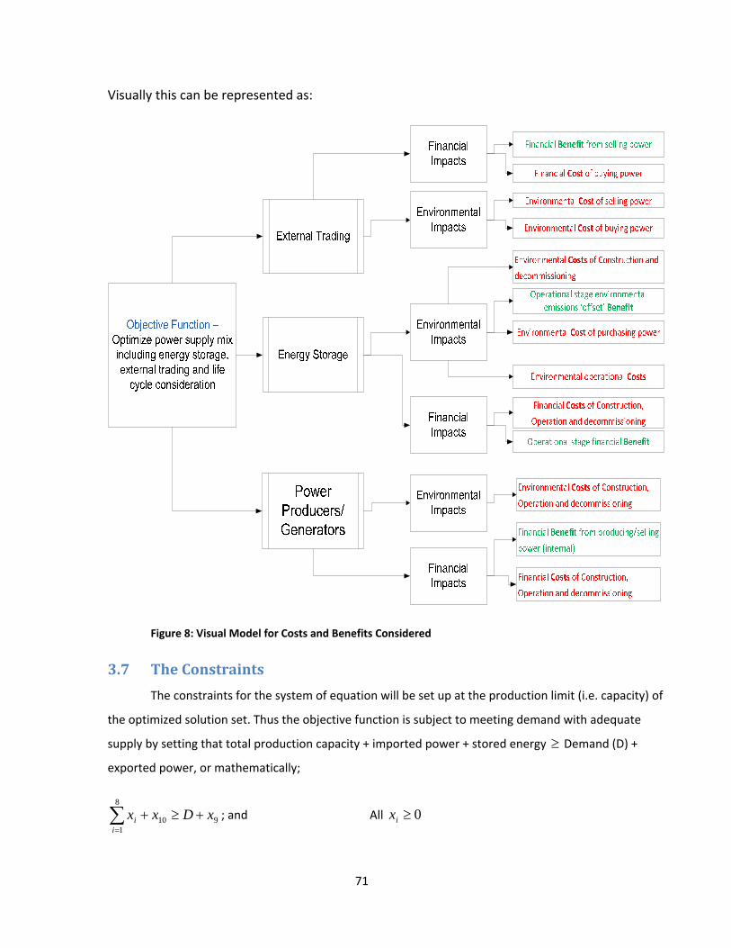
71

Visually this can be represented as: 

 

Figure 8: Visual Model for Costs and Benefits Considered 

3.7  The Constraints 

The constraints for the system of equation will be set up at the production limit (i.e. capacity) of 

the optimized solution set. Thus the objective function is subject to meeting demand with adequate 

supply by setting that total production capacity + imported power + stored energy ≥  Demand (D) + 

exported power, or mathematically; 

910

8

1xDxx

ii +≥+∑

=

; and                                         All  0≥ix  

  

72

3.8  Chapter Summary  

Accuracy was not the primary driver for the model developed and thus a linear (and 

averaged) approximation would suffice. The assumption regarding an aggregated energy cost 

for long life time infrastructure such as a nuclear or hydro station is crude and needs to be 

refined. Another assumption of note is that the model is constructed for a seasonal basis, since 

average power prices, renewable resource availability factors and consumption patters are best 

represented on a seasonal basis. Economic assumptions regarding present worth factors had 

also been addressed.  The objective function constructed was: 

Minimize {Costs – Benefits} 

Minimize {Financial Costs of Construction, Operation and decommissioning + Environmental 

Costs of Construction, Operation and decommissioning – Financial Benefit from 

producing/selling power (internal) + Environmental Cost of selling power + Environmental Cost 

of buying power + Financial Cost of buying power – Financial Benefit from selling power 

(external) + Financial Costs of Construction, Operation and decommissioning + Environmental 

Costs of Construction and decommissioning + Environmental Cost of purchasing power + 

Environmental operational Costs– Operational stage environmental emissions ‘offset’ Benefit – 

Operational stage financial Benefit } 

Subject to: Total production capacity + Imported power + Stored energy ≥  Demand (D)  

KEY ‐ Colour pertains to:   Generator/Power Producer   

Importing/Exporting Power   

Energy Storage 

  

73

4. Interpretation and Model Critique 

4.0  Chapter Introduction 

  The following chapter concludes the work by analyzing the model developed. It explores 

how the model may be calibrated, specifically for the Ontario market and what kinds of impacts 

can be expected for varying degrees of freedom. In particular, the sensitivity analysis 

recommends the cost of carbon, the EIO‐LCA sector selection, the network loss coefficient and 

the averaged real emissions to be variables towards a sensitivity analysis. The work considers 

future enhancements of the model with respect to reliability and risk mitigation that could be 

incorporated.  The use of the model as a policy tool is also examined. The work concludes by 

answering the question posed earlier regarding the evaluation of tradeoffs. The findings 

emphasize the need for strategic development with respect to technical and political solutions.  

 

 

 

 

 

 

 

 

 

 

  

74

4.1  Linear Program Characteristics  

  The objective function was set up as minimization linear program. The main reason for 

this is that the minimization problem is easier to construct, assimilate and solve. The equivalent 

dual of the problem could be stated as a standard primal maximization if the user required. The 

solution set for the problem does need further exploration however, in order to gauge the 

tradeoffs. Once the coefficients for the problem are known, the range of variation for the 

sensitivity analysis can be further elucidated. 

4.1.1   Model Analysis  

  The optimization model depends significantly on the average energy price values for 

power trading as well as energy storage. Since the average values change with seasonal 

variations, the optimization will need to run at least once for every season. For example, the 

expected changes from summer to winter will be a lower average selling rate during off‐peak 

winter loads versus a higher average price of buying power on hot summer days. These trends 

will shift the amount of storage capacity required and the environmental cost of selling and 

buying power.   

  When applied to all four seasons, this analysis will effectively generate four scenarios of 

optimal supply mix. External factors such as jurisdictional trading, power purchase agreements, 

transmission planning and outage requirements, contractual commitments and future planned 

generation can be used to determine the best option for energy storage in Ontario. Section 4.2 

examines in detail how the model can be enhanced with respect to other external factors. 

Businesses/the government can use the model to structure policy based on forecasts of 

demand and planned generation. Since the policy is based on the eco‐environmental objective 

function, it is strategic and demonstrates the most efficient way to spend the province’s 

opportunity dollar. Section 4.3 describes this case.  

4.1.2   Model Calibration  

  Before the model can be used for planning purposes, however, it needs to be calibrated. 

This can be achieved by constraining all the other known variables in the formula with the 

  

75

remaining energy trading variables left as unknowns. This forces the optimal supply mix to be 

efficient using energy trading. Optimization is also achieved by selecting a Carbon Cost  cT , and 

maintaining that cost . Alternatively, if the cost of carbon is set as a variable and all other 

variables are constrained to known values, there is no definitive solution.   A possible result in 

this circumstance is an inequality equation with an undefined solution.  

  If a reasonable cost of carbon is selected and the model runs with the trading variables 

as unknowns, the solution set of the trading variables will yield a ‘slack’ between the optimized 

and real world values. One can then use these values to constrain any other optimized solutions 

in the ‘business as usual’ case by maintaining the same ratio of ‘slack’ to any other variables.    

4.1.3   Sensitivity Analysis 

A sensitivity analysis for all assumed variables with indirect relationships is necessary. 

The recommended variables for sensitivity analysis for this formulation are: 

‐ Cost of Carbon  ( cT ) by ± 50$/Tonnes of CO2 or CO2 equivalents 

‐ Network Power Loss Approximation ( iN ) by ±  20% from the averaged value 

‐ The average of real emission coefficient ( ir  ) by ± 10% from the averaged value 

‐ Average buying and selling prices by varying the timescale from a single season to 

several years.  

‐ Sectors chosen in the EIO‐LCA. Since the model is linear, the environmental effects 

are averaged out over all the generation types. The environmental effects 

approximated using the EIO‐LCA tool for nuclear power may be much higher when 

compared to a real nuclear station, but this compensated for since the case may be 

reversed for coal. Varying the sectors may thus provide some value added sensitivity 

analyses. Since the costs are aggregated, the optimal solution’s true environmental 

footprint will be different from what the model predicts.  

  

76

The aforementioned variables will have the most direct bearing on the coefficients and 

objective functions. Performing a sensitivity analysis for them therefore alerts the user to which 

variables produce the most disturbances from the original set of optimized values.  

4.1.4   Model Adaptability 

The model is adaptable in that the mechanism and logic to assemble the formulation to 

evaluate tradeoffs is widely applicable. One can apply the same logic to different jurisdictions 

so long as the trends between price and demand remain similar and the EIO‐LCA is relevant.  

  It is possible to calculate the assumed cost of carbon. Depending on the coefficients and 

the inequality, a solution is not guaranteed. The model nevertheless provides a gauge with 

which to benchmark future work. If the model were run for different planning scenarios by 

specifying varying demands and planned generation, the inherent cost of carbon can be 

calculated and could be used as an environmental performance indicator for each of those 

scenarios. As a benchmark, the higher the inherent cost, the lower our reliance on fossil fuel 

based generation.  

4.2.1  Policy Planning and Predictability 

In addition to yielding an optimal supply mix, the author intends the model as a policy‐

planning tool.  Scenario analyses would yield a change in optimal supply mix to varying inputs. 

The predictability of the tool is driven by the ability of the EIO‐LCA to forecast environmental 

impact, the historical averages of construction, operation, decommissioning and energy retail 

costs, and the averaged network and other loss coefficients. These factors vary linearly as they 

are assumed to be proportional to capacities of the resources they factor into; hence the 

average calculation is valid. Real projects vary greatly, however,   from the averages calculated.  

Future technology improvements due to transmission planning, or efficient technologies may 

render the averaged calculations inaccurate. A more accurate representation of these factors 

would serve to yield better aggregate data and a relatively improved performance indicator. 

The model could also be expanded so that instead of aggregate data, individual projects across 

the network could be represented as such. In either case, the increase in accuracy is traded‐off 

  

77

against the level of complexity of the model. As a policy‐planning tool, the model would be run 

for several scenarios and the scenario that best represents the province’s direction can be 

invested in through artificial policy drivers1.  

If, for example, the scenario that included a significant increase in energy storage was 

desired, then policies could be crafted that would attract investment in the industry. 

Furthermore, the government could customize and/or limit the level of investment and 

incentives by performing a sensitivity analysis to evaluate the environmental and financial 

tradeoffs. The model would provide an indicator of when artificial drivers would suffice to give 

enough momentum to the industry to invest in energy storage or the desired generation type. 

The policy would therefore avoid over allocating resources to the cause since the costs and 

benefits are predictable. Predetermination of alternatives however still precedes the scenario 

planning and policy restructuring. The desired/most effective allocation of resources is 

nevertheless possible for any predetermined state of investment through the optimization 

process.  

4.2 Enhancement of the Model and Recommendations 

The paper has already examined some factors to enhance the model. Incorporation of 

risk mitigation, reliability and resiliency tradeoffs within the model are highly recommended. 

While these factors are enormously important, quantizing and representing them as economic 

terms is challenging. A more detailed and complex model may incorporate such considerations 

but may lack the ability to balance sustainability or environmental concerns with respect to 

optimization. The challenge is to relate both factors in a manner that allows the user to trade 

one benefit or cost for another. A simple example of such a tradeoff is the environmental 

impact of transmission infrastructure. One might ask for example, what levels of environmental 

impacts are deemed acceptable for an increase in reliability of the transmission network?  

The environmental impact for this model was limited to CO2 emissions, yet other 

impacts such as land use, waterway or drainage basin contamination, other environmental                                                             1 The FIT program is an artificial driver based on Ontario’s policy to be greener. Policy on taxing carbon, investing in electric vehicles, or even policy in terms of public transit usage, could all be used as effective tools. On the case of power production, subsidies, taxes and long term agreements are all artificial drivers. 

  

78

emissions, as well as indirect impacts such as noise pollution could all be included. The 

challenge for the formulation of the objective is incorporating them all on a common basis for 

comparison. The model used an economic approach to quantify the costs and benefits, yet 

other approaches are possible. Minimizing total energy use for a given level of utility was briefly 

considered. The challenge with respect to total energy use is to be able to distinguish and 

assess the impact of energy harvested from coal as opposed to energy harvested from wind. An 

energy break‐even based formulation was also considered but the challenge of classifying 

environmental impacts would remain. It is possible to weight factors in classifying energy usage 

as ‘good’ or ‘bad’ with non‐renewable sources of energy weighted heavier or penalized in the 

formulation. This approach was not adopted since it would require assuming or establishing 

weighting factors for all differing types of generation. The current formulation only assumes the 

cost of carbon  cT  as the common environmental taxation factor. Incorporating other types of 

environmental impacts using an energy analysis approach would present analogous challenges.  

Another area for future research includes improving data collection. As noted earlier, 

many of the coefficients are simple averages, not fully expounded here in favour of developing 

a useable framework. The creation of this basic framework lays the foundation for a project‐by‐

project basis that would significantly increase the accuracy of the model. The first step would 

be to weigh averages for several variables. The  ir values that represent the real emissions from 

power plants as well as the network power loss approximation factor iN  could be based on 

weighted averages as opposed to simple ones. The form of accounting for transmission factors 

could also be improved. If classification of the transmission network into a manageable number 

of known power‐line types for the entire network were possible, the objective could be 

reformulated to include and minimize transmission costs simultaneously.  The relationship 

between the increase in number of generation projects or capacity, and a corresponding 

increase in transmission infrastructure will need to be established nonetheless. The 

environmental transmission costs could be estimated from the average construction cost based 

on the type of transmission power‐line classification chosen. Note that the ‘value‐add’ from this 

approach will not be useful in optimizing the network from a technical perspective but one 

  

79

could nonetheless approximate the tradeoffs between transmission and generation. This new 

formulation could indicate where the public’s opportunity cost is best spent with respect to an 

environmental perspective.  

The proposed model’s capacity factors for intermittent sources such as wind and solar 

have been left out of the formula as explained in the assumption section 3.4.2. The ideal 

representation of intermittent sources would be through a probabilistic or stochastic function 

of resource availability. The model could be reconstructed to incorporate stochastic flows with 

a corresponding change in solving methodology. The decision to model intermittent resource 

availability as a stochastic phenomenon, or a discrete variable will depend on the usability of 

the assembled formulation. If solving the problem requires significant analysis and 

computational power, there must be a corresponding increase in the utility of the tool. The 

accuracy of the results based on using discrete variables of historical averages however, should 

suffice in terms of establishing a strategic policy direction. 

The model can also been adapted to minimize cost based on power capacities [MW], as 

opposed to life time energy costs [$/MWh]. In that case the variables would translate to total 

capacity [in terms of MW] of a particular generation type. It is highly recommended that this 

approach also be considered for future work.    

4.3  Integrated Discussion and Conclusion 

  The work began by discussing how Ontario could improve its socio‐economic 

performance using a benchmark performance index. In the context of energy generation and 

procurement planning, the 2009 Green Energy Act was introduced. Yet the lack of benchmarks 

prior to the Act may have resulted in a non‐strategic allocation and development of the present 

generation supply mix. The Act still does not propose any real benchmarks, performance 

criteria or policy goals it would like to meet. The instability of energy prices in Ontario, the lack 

of energy storage and the increasing energy industry related provincial debt, demonstrate the 

lack of non‐strategic development and the need for an optimized model for development.  

  

80

The work analyzed the OPA’s supply mix advice for procuring power, and compared the 

advice with the present power systems of Germany and Denmark, upon which the advice was 

based. The supply mix advice report detailed Ontario’s resource availability yet the life cycle 

weighting consideration could have been more effectively incorporated. Furthermore, while 

the aspects of increasing renewable energy in the province were included in the German and 

Danish models, other aspects such as transmission planning, energy storage and policy were 

ignored. The power sectors for both Germany and Denmark are presented as case studies and 

the lessons learned could prove significant for Ontario. The fluctuation in Denmark’s power 

prices, the cash‐strapped German energy consumers, the reversal of the nuclear phase‐out 

legislation, and the renewed need for investment in Danish wind power are all lessons 

identified for Ontario to execute any planning course of action. The integrated view of the 

model allows energy storage, energy trading and sustainability considerations to be taken into 

account while simultaneously optimizing, and thus recommending the energy based capacities 

for each generation type. Though the recommended strategy may be sound, the government 

may need to provide policy‐based drivers as incentives to pursue the strategy. These policies 

must be carefully constructed, lest the unintended consequences such as dwindling incentives 

for wind power in Denmark become a reality for Ontario.  The model is able to evaluate energy 

storage as a function of economic and environmental, costs and benefits, thus providing a 

potential baseline for the OPA with respect to the new IPSP, by which it is possible to evaluate 

the potential for energy storage. 

The optimization logic can also be more broadly applied. The model allows for an 

assessment of the questions posed regarding evaluating the seemingly incongruent economic 

tradeoffs between environmental impacts and supply mix. It is now possible to place an 

economic value on greenhouse gas emissions as well as evaluate the most cost – efficient 

opportunities. This narrow definition can be expanded however, to include other economic or 

social goals. While the previous section discussed this concept, it is possible for other social or 

economic systems to implement the mechanism to integrate environmental considerations 

analogously for their respective goals.  

  

81

Consider that the economic benefits of building a hospital or school can now be evaluated 

together with environmental impacts. Or that the economic and monetary values associated 

with greenhouse gas emissions can be compared with those of health care. In this sense, one 

may compare the opportunity cost of providing healthcare versus reducing smog effects. Such 

an integrated and strategic view will ensure that the most effective options are reinforced with 

measurable benchmarks and progress indicators. While the model developed was constructed 

for the power sector, other sectors can adopt the application of the assembling logic of the 

objective. The objective has tried to represent the region between the extremes of economic 

and environmental cost efficiency. It is in the gray areas between the extremes that the optimal 

solutions usually exist and it is precisely such considerations that remain unengaged. Further 

work as described earlier is recommended to develop the model, both within the power sector 

and without. The application of the model to other subject areas will generate feedback to 

enhance this one. Broader application of this model is therefore advantageous and encouraged. 

  

82

5.0 Bibliography (EIA) US Energy Information Administration. International Electricity Installed Capacity http://www.eia.doe.gov/emeu/international/electricitycapacity.html (accessed March 24th 2010) 

 Bode, Sven. Nucs down in Germany—Prices up in Europe? Energy Policy Volume 37, Issue 7, July 2009 Pages 2492‐2497   

Brundtland, Hariem G. Report of the World Commission on Environment and Development: Our Common Future. Environmental Policy and Law, Volume 14, March 1985  Carnegie Mellon, University of and Toronto, University of “Theory and Method behind EIO‐LCA” http://www.eiolca.net/Method/eio‐lca‐method.html (accessed March 24th 2010)  Denholm, Paul and Kulcinski , Gerald L. Life cycle energy requirements and greenhouse gas emissions from large scale energy storage systems. Energy Conversion and Management, Volume 45, 2004. Pages 2153‐2172  Duffield, John S. Germany and energy security in the 2000s: Rise and fall of a policy issue? Energy Policy Volume 37, Issue 11, November 2009, Pages 4284‐4292  

Fairley, Peter. IEEE Spectrum. “Germany’s Green Energy Gap” http://spectrum.ieee.org/energy/policy/germanys‐green‐energy‐gap/0 (accessed March 24th 2010)  Finnveden, Goran et al Recent Developments in Life Cycle Assessment Journal of Environmental Managament. Volume 1, Issue 21, 2009  Furlong, Ray. “Germany begins to turn against Wind”. British Broadcasting Corporation http://news.bbc.co.uk/2/hi/europe/3148422.stm (accessed March 24th 2010)  Jacobsen, Henrik Klinge and Zvingilaite, Erika Reducing the Market Impact of Large Shares of Intermittent Energy In Denmark Energy Policy, Published 23rd Feb 2010  Laurent, Viguier L. Babiker, Mustafa H. Reilly, John M. The costs of the Kyoto Protocol in The European Union Energy Policy, Volume 31, Issue 5, Pages 459 ‐ 481 

Lipp, Judith Lessons for effective renewable electricity policy from Denmark, Germany and the United Kingdom Energy Policy v35 issue 11, Nov 07, pgs 5481‐5495, 

Lyle, Michael. Ontario Power Authority  “File No. EB‐2007‐0707” lhttp://www.powerauthority.on.ca/Storage/96/9159_OPA_Letter_EB‐2007‐0707_20090312.pdf (accessed March 24th 2010)) Ontario Ministry of Energy and Infrastructure. “ReNew Onatrio” http://www.mei.gov.on.ca/en/infrastructure/renew/ (accessed March 24th 2010)  Pahle,Michael. Germany’s dash for coal: exploring drivers and factors, Energy Policy , Volume 37, Issue 7  Feb 5th 2010  Smitherman,  George.  Legislative  Assembly  of  Ontario  “Bill  150  ‐2009  –  An  Act  to  enact  the  Green EnergyAct,2009“http://www.ontla.on.ca/web/bills/bills_detail.do?locale=en&BillID=2145&detailPage=bills_detail_the_bill&Intranet=” (accessed March 24th 2010))  

  

83

Spears, John. “Toronto Hydro debt move alarms privatization foes”. Toronto Star. http://www.thestar.com/business/article/784286‐‐toronto‐hydro‐debt‐move‐alarms‐privatization‐foes (accessed March 24th 2010)   (IESO) Independent Electricity System Operator. “ Supply Overview” http://www.ieso.ca/imoweb/media/md_supply.asp (accessed March 24th 2010)   (OPG) Ontario Power Generation. Sir Adam Beck Pump Generating Station. http://www.opg.com/power/hydro/niagara_plant_group/adambeckpgs.asp (accessed March 24th 2010)  Bruce Power “Energy for a New Generation” http://www.brucepower.com/pagecontentU12.aspx?navuid=29 (accessed March 24th 2010)  Czuczka, Tony Germany’s Nuclear power Extension Split’s Merkel’s Government. Bloomberg Businessweek http://www.businessweek.com/news/2010‐02‐08/germany‐s‐nuclear‐power‐extension‐splits‐merkel‐s‐government.html (accessed March 24th 2010)  Ontario Electricity Financial Corporation “Debt Management” http://www.oefc.on.ca/debtmanage.html  (accessed March 24th 2010)  Ontario Electricity Financial Corporation “Management of Power Purchase Agreements” http://www.oefc.on.ca/ppa.html (accessed March 24th 2010)  Ontario Ministry of Finance “Ontario’s Long‐Term Report on the Economy. Chapter 5: Addressing Ontario’s Infrastructure Gap” http://www.fin.gov.on.ca/en/economy/ltr/2010/ch5.html (accessed March 24th 2010)  Ontario Power Authority “Renewable Energy Feed‐in Tariff Program” http://fit.powerauthority.on.ca/Page.asp?PageID=122&ContentID=10195&SiteNodeID=1098&BL_ExpandID=259 (accessed March 24th 2010)  OPA, Ontario Power Authority “ Supply Mix Advice Report” http://www.powerauthority.on.ca/Storage/18/1338_Part_1‐1_Supply_Mix_Summary.pdf (accessed March 24th 2010)  2009, S.O. 2009, c. 12, Schedule A [Green Energy Act], CanLii (accessed March 24th 2010)