Online Supplementary Material Stochastic expression ... · Online Supplementary Material Stochastic...

Online Supplementary Material Stochastic expression dynamics of a transcription factor revealed by single-molecule noise analysis Zach Hensel1*, Haidong Feng2*, Bo Han2, Christine Hatem1, Jin Wang2,3,4, Jie Xiao1 1 Department of Biophysics and Biophysical Chemistry, Johns Hopkins University School of Medicine, Baltimore, MD 21205, USA. 2 Department of Chemistry and Physics, SUNY Stony Brook, Stony Brook, NY 11794, USA. 3 State Key Laboratory of Electroanalytical Chemistry, Changchun Institute of Applied Chemistry, Changchun 130022, P.R. China. 4 College of Physics, Jilin University, Changchun 130021, P.R. China. * These authors contributed equally to this work. Corresponding authors: [email protected], [email protected]

Nature Structural & Molecular Biology doi:10.1038/nsmb.2336

Supplementary Figures

Supplementary Figure 1. CoTrAC method validation. (a, b) Typical Western blots used to quantify the molar ratio between separated Venus-Ub and CI. Cells harbor plasmid pZH051–tsr and expresses Venus-Ub-CI in the absence (a, lanes 1-3; b, lanes 2-4) or presence (a, lanes 4-6; b, lanes 5-7) of Ubp1. In the anti-GFP blot (a), lane 7 is the negative control strain DH5α; lane 8 is loaded with 1 ng purified GFP. In the anti-CI blot (b), lane 1 is the negative control strain DH5α and lane 8 is the wild-type λ lysogen JL5932. (c) Typical blot used to quantify Tsr-Venus-Ub-CI expression. In the anti-YFP blot, the λWT strain lacking Ubp1 expression is loaded in 10-fold excess to be visible. The uncleaved Tsr-Venus-Ub-CI band is still much dimmer than the bands for λWT and λr3, indicating that the removal of the Tsr-Venus-Ub reporter from the N-terminus of CI activates CI. The anti-CI blot shows that a wild-type λ lysogen, JL5392, had a similar CI expression level to λWT. (e) CI expression levels in λWT and λr3 with and without cro are indistinguishable, showing that cro expression in λWT and λr3 is unlikely to contribute to differences observed in λb, where cro is deleted.

ȜWT0

0.20.40.60.81

1.21.41.6

&,�(

[SUHVVLRQ��UHODWLYH�WR�Ȝ

WT )

Steady-state expression with and without cro

Ȝr3

– cro+ cro

ȜWT Ȝ– Ȝr3 JL53920

0.5

1

1.5

2

2.5

([SUHVVLRQ��UHODWLYH�WR��Ȝ

WT )

Single Cell Fluorescence

Westerns

Molecules/Generation

d

��îȜWT ȜWT Ȝ– Ȝr3 GFP

ȜWT Ȝ– Ȝr3JL5392

+Ubp1

+Ubp1

Ctrl

Ant

i-YFP

Ant

i-CI

c

100

2735

5570

Venus-Ub-CI

Venus-Ub

GFP

1 2 3 4 5 6 7 8– UBP1 + UBP1a

Venus-Ub-CI

b

100

2735

5570

Anti-CIAnti-GFP

CI

Venus-Ub-CI

e

Mol

ecul

ar W

eigh

t (kD

a) 1 2 3 4 5 6 7 8– UBP1 + UBP1


Supplementary Figure 2 Timelapse image analysis methods (a) Brightfield images are segmented using a custom MATLAB routine. Images are filtered before being segmented (using a Laplace-of-Gaussian method). Objects above a size threshold are retained. Segmentation is manually adjusted and cells in movies are assigned to cell lineages. (b) An example lineage tree corresponding to the colony in a. (c) Fluorescence imaging routine described in Online Materials and Methods. (d) Integrated fluorescence intensity distribution of spots (N=1526) detected in time traces of λ–. The histogram is well fit by the sum of two (purple) or three (green) normal distributions with quantized means of ~0.05. A single normal distribution (red) does not fit the data well. (e) Histograms of cell generation lengths in minutes show that cell growth is similar in all strains and that the difference in CI expression levels in the four strains is not the result of different cell generation lengths. (f) For all cell-cycle data, the number of molecules detected for raw (solid) and cell-cycle-corrected (dashed) time traces are binned by the fraction of a cell cycle elapsed (e.g. an observation at 15 min in a 60-min cell cycle maps to 0.25) and averaged.

0 0.2 0.4 0.6 0.8 1

2468

101214

Fraction of cell cycle elapsed

Mol

ecul

es p

er 5

min Ȝr3

ȜWT

Ȝí

Generation length40 60 80 100 1200

0.04

0.08

0.12

Freq

uenc

y

ȜbȜWT Ȝr3 Ȝ–

Spot intensity (AU)

Freq

uenc

y

a b

35 1 – 6

c

e

0.180.02

1.0

0.08

0.04

0.06 0.10 0.14

f

d1 2 3 4 5 6 1 – 6


Supplementary Figure 3 Time-dependent analysis of CI expression noise (a) The noise at each time window was calculated as the average of noise of all possible time window positions along long CI production time traces for λr3. The averaged noise from all time traces (circles) at each time window is then plotted against the length of each time window. The population noise level is plotted as a dashed line. (b) Autocorrelation of the four strains using long time traces spanning multiple cell generations. Solid curves are single exponential fits for λWT

and λr3 with apparent decay half times of ~20 min and 50 min, respectively. Single exponential fits to λb and λ– resulted in poor fitting—possibly due to the low and autocorrelation values and large error ranges. (c) The solid black curve is the fit using y=A/x+B. The dotted curve is the fit by fixing the intrinsic Fano factor A=1. The dashed curve is fit by fixing the extrinsic noise term, B=0. (d) Circles denote the noise curve calculated from the entire data set (N=523); triangles are from cells within 1.5 standard deviation of the mean CI production rate per 5-min (N=464); and squares are from cells within 1 standard deviation (N=377). Solid curves are fits using y=A/x+B. The fitted intrinsic noise, A, changes little (2.9, 2.7 and 2.7 for circles, triangles and squares, respectively). In contrast, the fitted extrinsic noise, B, changes substantially (0.07, 0.04, and 0.02, respectively). (e) Without subtracting the memory, the resulting noise curve fitting in λWT (dashed gray) is significantly poorer (chi-square increased more than 20-fold) than that with the memory subtracted (solid black).

0.20

0.25

0.30

0.35

50 100 150 200Time window (min)

a

0.1

0.2

0.3

0.4

0 10 20 30 40 50

total noisememory subtracted

Mean number of CI moleculesproduced in time window (!)

b

c d

e

!WT !r3

!b !–

Noi

se ("

2 /!)

2

Noi

se ("

2 /!)

2N

oise

("2 /!

)2

Noi

se ("

2 /!)

2

0 10 20 30 40 50 60 700.00

0.05

0.10

0.15

0.20

0.25

0.30

0.35



0.05

0.10

0.15

0.20

0.25

0.30

0.35

0 10 20 30 40 50 60 70

-0.1

0.0

0.1

0.2

0.3

0.4

0 50 100 150 200Lag time (min)

Auto

corre

latio

n (C

(!)/C

(0))

!


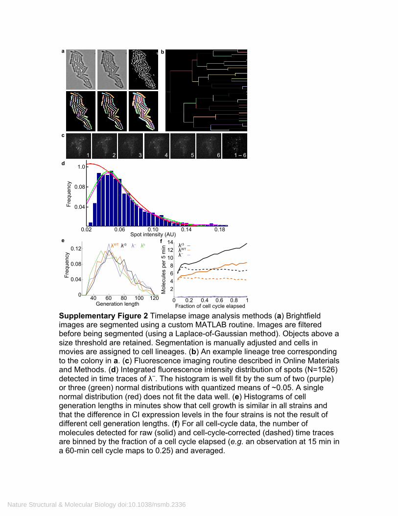
Supplementary Figure 4 Additional analysis of fluorophore-maturation effect and burst-like protein production (a–c) Noise curve fitting by considering the maturation effect for strain λr3 (a), λb (b) and λ– (c). The circles are the noise at each time window and the solid curve is the fitting using Eq. 40 in Supplementary Note 2. The fit values are reported in Supplementary Table 4. (d) Histogram of numbers of expression bursts in a fixed time window for λ– (N=217 single-generation time traces truncated at 45 min—the shortest cell-cycle time). The histogram was fit with a Poison distribution (solid curve) with an average bursting frequency of ~0.6 burst per cell cycle.

Time window (min) Time Window (min)

0.2

0.6

1.0

10 20 30 40

5

10

15

20

10 20 30 40Time Window (min)

a b c

0.10

0.20

0.30

10 20 30 40

50

100

150

Occ

uren

ces

Number of CI expression bursts

Noi

se (!

2 /")

2

Noi

se (!

2 /")

2

Noi

se (!

2 /")

2

d

0 1 2 3 4


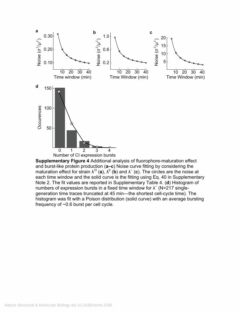
Supplementary Tables Supplementary Table 1: Bacterial strains used in this study. Strain Genotype Source JL5392 JL2497 lysogenized with JL163 Gift from John Little

λWT MG1655 (cI–rexB)::tsr-venus-ub-cI/pCG001 This work

λr3 λWT OR3-r3/pCG001 This work λb λWT cIM1L Δcro This work λ– λWT cIM1L/pCG001 This work


Supplementary Table 2. Noise is unaffected by correcting the CI production rate for the cell-cycle effect. The data below were calculated using either uncorrected raw or linearly corrected time traces of CI production in 5-min frames.

λr3 λ– λb λWT

Uncorrected data

µ 11.6 0.095 2.9 7.7 σ2/µ2 0.32 18.3 0.96 0.40 σ2/µ 3.7 1.7 2.8 3.0

Corrected data

µ 7.8 0.063 1.9 5.2 σ2/µ2 0.32 19.4 0.96 0.39 σ2/µ 2.5 1.2 1.9 2.0

1.44σ2/µ 3.6 1.8 2.7 3.0


Supplementary Table 3. Noise properties of the four strains calculated using different methods as described in Supplementary Note 1. All results are calculated using cell-cycle-corrected data.

λr3 λ– λb λWT Total noise 0.32 19.4 0.96 0.40

Intrinsic noise estimated from

noise curve 0.25 19.0 0.87 0.36 correlation

pairs 0.22 18.7 0.81 0.25

cell-cycle average 0.23 17.2 0.80 0.27

Intrinsic Fano factor 2.9 1.8 2.4 2.7

Extrinsic noise estimated from

autocorrelation 0.09 0.6 0.10 0.08 noise curve 0.07 0.6 0.10 0.04 correlation

pairs 0.09 1.1 0.13 0.14

cell-cycle average 0.09 2.2 0.16 0.13


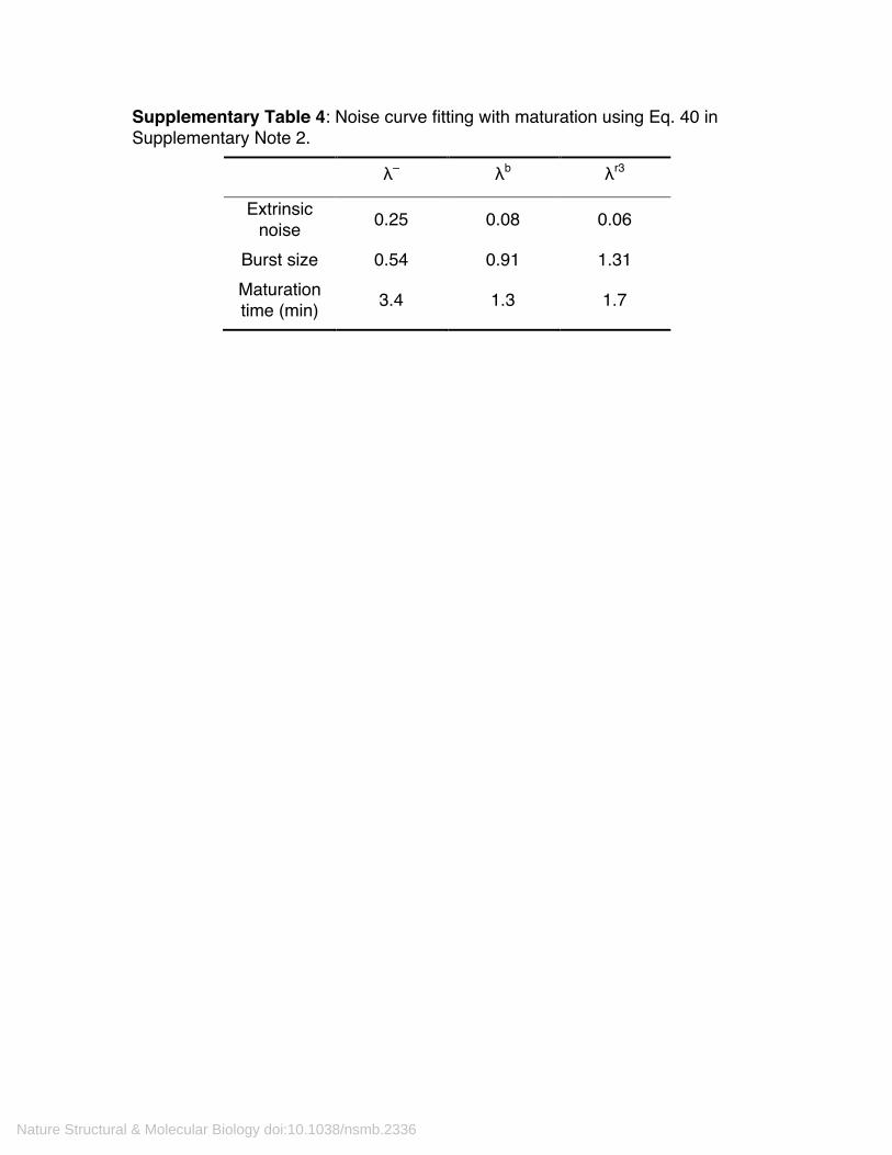
Supplementary Table 4: Noise curve fitting with maturation using Eq. 40 in Supplementary Note 2.

λ– λb λr3

Extrinsic noise 0.25 0.08 0.06

Burst size 0.54 0.91 1.31 Maturation time (min) 3.4 1.3 1.7


Supplementary Table 5: Primers used in strain construction detailed in Online Materials and Methods. Primer Sequence P1 GACGATGGATCCGGGCTGGAATGTGTAAGAGC

P2 GATTGGATCCTGCGTCCTGCTGAGGTGC

P3 CATAGCAATTCAGATCTCTCACCTAC

P4 ATGCGCCGACCAGAACAC

P5 GCATACTCGAGATGCAGATTTTCGTCAAGAC

P6 ACCACCTCTTAGCCTTAGCACAAGATGTAAGG

P7 ATGAGCACAAAAAAGAAACCATTAACAC

P8 CTATCTCGAGTTAAATCTATCACCGCAAG

P9 CGGGCTCGAGAGGAAACAGCTATGTTAAAACGTATC

P10 CTAACCCGGGGTGTAGGCTGGAGCTGCTTC

P11 CATACCCGGGAACCATCTGCGGTGATAAATTATC

P12 CATTCTCGAGTATCACCGCAAGGGATAAATATCTAAC

P13 CAATACGCAAACCGCCTCTC

P14 GGCTGCGGTAGTTCAGGCAG

P15 GCACGGTGTTAGATATTTATCCCTTGTGGTGATAGATTTAAC

P16 GTTAAATCTATCACCACAAGGGATAAATATCTAACACCGTGC

P17 TGCTAAGGCTAAGAGTGTGTCTGAGCACAAAAAAGAAAC

P18 ACGATTCCGATTCTCCACCAGACTCGTGTTTTTTCTTTG

P19 TGTACTAAGGAGGTTGTATGAACAACGCATAACCCTGAAA

P20 TTTCAGGGTTATGCGTTGTTCATACAACCTCCTTAGTACA

P21 AGCAAGGGCGAGGAGCTGT

P22 CATAGCTGTTTCCTGTGTGCTCG


Supplementary Note 1 Supplemental data analysis CI expression is not significantly affected by Cro in λr3 and λWT

We measured the steady-state level of CI expression by integrating single-cell fluorescence for strains λr3 and λWT as well as in equivalent strains with cro removed by site-directed mutagenesis as in λb. Supplementary Fig. 1e shows that expression in the two strains in the absence of cro is not significantly different from that in the presence of cro. Thus, differences in PRM activity between λb and λr3 are due to the inactivation of CI and not from any effect of Cro binding. Cell-cycle length distribution We generated histograms of the observed cell cycle lengths in time traces of all four strains and found them to be indistinguishable from each other within experimental uncertainties (Supplementary Fig. 2e). We did not use cells that have extremely short or long cell cycle lengths, which may be indicative of abnormal physiological states. For analyses discussed in the main text, we selected cells that have a cell cycle length between 45 and 100 min. Linear correction for cell-cycle dependence During the bacterial cell cycle, the number of chromosome copies, and thus the copy-number of a particular gene, doubles. We observed that, averaged over all time traces, the CI expression rate increased linearly throughout a cell cycle and doubled at the end of the cell cycle (Supplementary Fig. 2f). This linear increase is counterintuitive if one assumes that the expression rate should only double at the moment a gene is replicated. Nevertheless, a number of studies have observed similar effects1, 2. This effect could be due to reasons that our estimation of when a cell cycle begins and ends is inexact, obfuscating any discrete increase in expression, and/or that the time of gene doubling varies substantially between cells. We corrected the cell-cycle dependence of CI expression by assuming that the rate of CI production at the end of cell cycle exactly doubles that at the beginning of the cell cycle to create a corrected time series of CI expression per 5 min, n(t), from the observed time trace, n ′(t), given a cell-cycle length of T:

n(t)= n '(t)1+ t T

. (1)


All the data reported in this work are corrected using Eq. 1. The effect of the linear correction on noise and Fano factor The linear correction (Eq.S4) for cell-cycle dependence does not change the noise σ2/μ2 because the mean, μ, and standard deviation, σ, are scaled in the same way. However, the linear correction will reduce the Fano factor, σ2/μ. For example, for a set of random numbers n with a Fano factor F, if each number n is divided by a factor a, the resulting Fano factor will be F/a:

aF

n

nn

aan

an

an

=−

=

−⎟⎠⎞⎜

⎝⎛

22

22

1

. (2)

For a CI production time trace, if the cell-cycle-dependent increase in CI production rate is caused by increased expression frequency but not the size of each expression event, the true Fano factor, which we show to be determined by burst size but not frequency in Supplementary Note 2, should remain a fixed value. However, the mathematical treatment to correct the cell-cycle dependence will cause the Fano factor directly calculated from the corrected data to be artificially smaller than the true one in the absence of cell-cycle dependence. Further, since the number of CI molecules measured at a particular time, n ′(t), is corrected using a different coefficient a(t) (between 1 and 2) according to its position in the cell cycle, the true Fano factor can not be simply calculated by scaling the Fano factor with a fixed value as shown in Eq. 2. In the following we show that the true Fano factor of CI production in the absence of correction for cell-cycle dependence, F ′, should take the form of F ′= F/ ln(2), where F is the Fano factor directly calculated from data after linear correction. We assume a protein production time series that has a fixed Fano factor, F ′, but an average protein production rate that doubles linearly through a cell cycle of length T. In the whole series, we approximate that during the time interval from mt to (m+1)t the expression frequency is constant. Therefore, the average number of protein molecules <n ′(t)> produced during such a time window can be expressed as:

ntatn )()(' = . (3) Here, the coefficient is a constant with the value Ttta /1)( += , and <n> is the


mean protein production rate in the absence of cell-cycle dependence. Correspondingly, the Fano factor calculated using data from the same time window equals F ′ with )('/))(')('(' 22 tntntnF −= . After linear correction we have a new time series:

)(/)(')( tatntn = , ntatntn == )(/)(')( . (4) In principle, the true Fano factor F ′ can be calculated by dividing CI production time traces into multiple time windows such as 1st, 2nd, and 3rd 5-min windows, and only using data in the same time window from different cells. However, this treatment will reduce the available sample size, leading to an increased uncertainty in the calculated Fano factor. In addition, variations in cell-cycle length (Supplementary Fig. 2e) would complicate this calculation. Therefore, we take the following approach by showing that the total variance of the time series after linear correction is the variance at each time window integrated over all available time windows:

σ 2 =1T

dt0

T∫ n '(t)

a(t)"

#$

%

&'

2

−n '(t)a(t)

2)

*++

,

-..=1T

dt0

T∫ F '

an 'a

=F ' nT

dt0

T∫ 1

a(t)

= F ' n ln 2( )⇒ F = σ2

n= ln(2)F '

. (5)

Eq. 5 shows that the true intrinsic Fano factor, F ′, can be calculated from the Fano factor after correction, F, as: F’ = F/ln(2). All the Fano factors we reported in Table 1 are adjusted using the 1/ln(2) factor. The intrinsic Fano factors listed in Table 1 are the fitted intrinsic Fano factor obtained from the noise curve, then adjusted using the 1/ln(2) factor. Presence of a slow variation in CI production rate We examined the time scale at which temporal fluctuations of a CI production time trace approach the population level. If there are no extrinsic differences between different cell lineages, the temporal noise of a CI production time trace would equal to that of the population at any given time. We calculated the noise in the CI production rate (number of CI molecules expressed per 5 min) using time windows of different lengths within individual long cell lineage traces. We then averaged the noises calculated using time windows of the same length from different cell lineages. The resulting mean noise is then plotted against the length of the time window used and compared with the population noise level. Supplementary Fig. 3a shows that the noise at


long time windows is larger than that at short time windows, indicating that variation within lineages is smaller than that between lineages. Furthermore, the noise gradually approaches population noise level in ~4 cell cycles, indicating that this noise operates on a time scale longer than a single cell generation. This observation is indicative of the presence of cell-to-cell heterogeneity, or extrinsic noise as termed in previous studies. The long time scale of extrinsic noise allowed us to approximate it as a constant on the time scale of one cell cycle. Calculation of autocorrelation We used time traces of single cell generations that are between 45 and 100 minutes long. To ensure that each cell has equal contribution to different time lags, we truncated all time traces at 45 min. We calculated the autocorrelation at different time lags, τ, for each time trace according to the following equation:

])(1[*])(1[)(*)(1)(,,,∑∑∑ +−⎟

⎠⎞⎜

⎝⎛ +=

jij

jij

jijj in

Nin

Ninin

NC τττ . (6)

Where index j is the jth cell and index i is the ith frame of data point in the time trace of cell j. ∑=

jiN

,1 is the total number of data pairs for a given time lag.

For λWT, we observed an autocorrelation decay time ~20 min. For the other three strains, we observed a rapid decay at the first 5-min time lag, and a relatively constant plateau at longer time lags. To verify whether these observations are still valid in long time traces, we computed autocorrelation of all the four strains using long cell lineages that span more than one generation. The resulting autocorrelation is similar to what was observed using single generation time traces. The time it takes for the autocorrelation to drop to half of the initial value at first time lag is ~20 min for in λWT, ~50 min for λr3, and difficult to estimate for λb and λ- because of their low correlation values with large error ranges (Supplementary Fig. 3b). The decay time for λr3 is significantly slower than that of λWT: it approaches the length of one cell cycle, consistent with the relative constant autocorrelation values calculated using single generation time traces (longest time window at 40 min). While we can also subtract this low correlation out from the total noise of λr3 as we did for λWT, it does not improve the noise curve fitting goodness significantly for λr3. Estimation of intrinsic and extrinsic noise using different methods We estimated intrinsic and extrinsic noise of the four strains using four different methods: autocorrelation, noise curve, correlation pairs, and a previously described method estimating extrinsic noise from averaged production over cell cycles3.


Autocorrelation: We computed the autocorrelation for CI expression per 5 min for each strain. For λr3, λ– and λb, we took the average of the autocorrelation values after the zero time lag as the variance of extrinsic noise and then divided it by the square of the mean CI production rate to estimate the magnitude of extrinsic noise. The autocorrelation of CI expression in λWT does not fall to zero quickly, so the extrinsic variance was taken as the average of the last two time lags. The extrinsic noise estimated from autocorrelation curve is higher than that obtained with noise curve analysis, because the autocorrelation curve is too short to reach the true plateau. Therefore, extrinsic noise estimations using this method can be regarded as the upper bounds of extrinsic noise. Noise Curve: For each time trace of a single cell generation between 45 and 100 min, we summed the total number of CI molecules nNt produced in N subsequent time windows using all possible time window positions. We then calculated the noise η2 in nNt obtained at the same time window from all time traces. Because the sample sizes at long time windows are smaller than those at short time windows, we truncated the noise curve at the 40-min time window. The resulting noise curve is fitted with function y=A/x+B. The intrinsic noise at 5-min time window is calculated using the fitted intrinsic Fano factor A adjusted using the 1/ln2 factor, and then divided by the mean expression level of CI at the 5-min window for each strain. The fitted value B is taken as the extrinsic noise according to main-text Eq. 4. Correlation pairs: We show in Supplementary Fig. 3a that extrinsic noise operates on a time scale of several cell cycles. Therefore, for two adjacent frames in a time series, the extrinsic noise can be approximated as constant. The difference in the number of CI molecules produced in the two adjacent frames can then be regarded as arising from intrinsic noise. The difference in the numbers of CI molecules produced in two non-adjacent time points then contains greater contribution from extrinsic noise. In an approach analogous to a previous method using two fluorescent reporters4, every pair can be regarded as a cell in which there are two reporters. The intrinsic and extrinsic noise can be estimated using equations:

21

2212

int 2

)(

nn

nn −=η and

21

21212

2 nnnnnn

ext

−=η . (7)

Here, n1 and n2 are the numbers of CI molecules produced in two adjacent time frames. For a time trace of CI production, all possible adjacent pairs are used in the calculation. We note that this method is valid only when each time frame is independent of adjacent time frames, i.e. there is no correlation. This assumption is reasonable for λr3, λ– and λb strains, but does not hold for λWT. As a result, the extrinsic noise of λWT estimated using this method is significantly higher than the


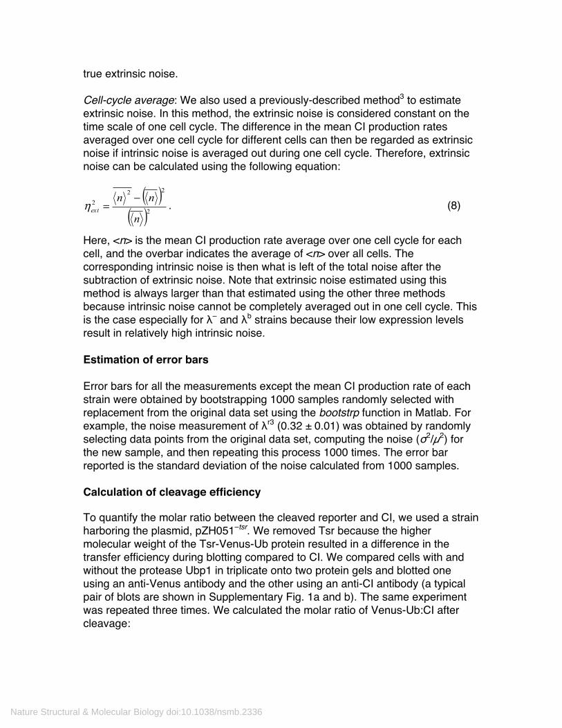
true extrinsic noise. Cell-cycle average: We also used a previously-described method3 to estimate extrinsic noise. In this method, the extrinsic noise is considered constant on the time scale of one cell cycle. The difference in the mean CI production rates averaged over one cell cycle for different cells can then be regarded as extrinsic noise if intrinsic noise is averaged out during one cell cycle. Therefore, extrinsic noise can be calculated using the following equation:

( )( )2

222

n

nnext

−=η . (8)

Here, <n> is the mean CI production rate average over one cell cycle for each cell, and the overbar indicates the average of <n> over all cells. The corresponding intrinsic noise is then what is left of the total noise after the subtraction of extrinsic noise. Note that extrinsic noise estimated using this method is always larger than that estimated using the other three methods because intrinsic noise cannot be completely averaged out in one cell cycle. This is the case especially for λ– and λb strains because their low expression levels result in relatively high intrinsic noise. Estimation of error bars Error bars for all the measurements except the mean CI production rate of each strain were obtained by bootstrapping 1000 samples randomly selected with replacement from the original data set using the bootstrp function in Matlab. For example, the noise measurement of λr3 (0.32 ± 0.01) was obtained by randomly selecting data points from the original data set, computing the noise (σ2/µ2) for the new sample, and then repeating this process 1000 times. The error bar reported is the standard deviation of the noise calculated from 1000 samples. Calculation of cleavage efficiency To quantify the molar ratio between the cleaved reporter and CI, we used a strain harboring the plasmid, pZH051–tsr. We removed Tsr because the higher molecular weight of the Tsr-Venus-Ub protein resulted in a difference in the transfer efficiency during blotting compared to CI. We compared cells with and without the protease Ubp1 in triplicate onto two protein gels and blotted one using an anti-Venus antibody and the other using an anti-CI antibody (a typical pair of blots are shown in Supplementary Fig. 1a and b). The same experiment was repeated three times. We calculated the molar ratio of Venus-Ub:CI after cleavage:


VenusantiCIUbVenus

CIantiCIUbVenus

CIantiCI

VenusantiUbVenus

CIUbVenus I

III

M −−−

−−−

−

−−

− ⋅= .

Here, I is the intensity of the protein band specified by the subscript. The superscript indicates whether the protein band was detected using an anti-Venus or anti-CI antibody. The averaged Venus:CI ratio was 1.1 ± 0.1. Based on the number of cells loaded in each lane (1.2 million) and the relative intensity of 1 ng of GFP, the cleaved samples in Supplemental Fig. 1a (lanes 4 to 6) contain approximately 7,000 Venus-Ub molecules per cell. No uncleaved band is seen at this high expression level, demonstrating the highly efficient cleavage by Ubp1. Quantifying CI expression via multiple methods Supplementary Fig. 1d shows the results of 3 parallel, independent methods of calculating CI expression. The results of our timelapse experiments (the number of CI molecules produced per generation) were compared to the integrated steady-state fluorescence intensity of single cells as well as the number of CI molecules expressed per cell calculated from immunoblots detecting either CI or YFP. To compare results from different methods, all expression levels were normalized to CI expression in λWT. When available, error bars represent the standard deviation of independent measurements using a particular method (measures of error are not always available; i.e. for λWT Western blots, expression levels are normalized to λWT measurements so error estimates are only available for other strains). We find that our single-cell, timelapse measurements are indistinguishable from alternative measurement methods within error. We also see that CI expression in a wild-type λ lysogen is comparable to that in λWT (~75% of λWT expression), indicating that CI should be near its wild-type concentration in experiments utilizing λWT, and thus subject to regulatory mechanisms relevant to λ lysogeny. Quantization of Venus intensity The distribution of Tsr-Venus-Ub fluorescent spot intensities for λ– is shown in Supplementary Fig. 2d. The mean intensity value also agrees with in vitro single-molecule measurement of purified Venus molecules. Note that low-intensity data (intensity less than 0.035) was not used in the fit due to the following considerations: (a) a number of single-molecule expression events (~10% assuming the distribution shown here) are too weak to be detected in YFP images. This is expected since photobleaching is generally an exponential process and some molecules will photobleach quickly; (b) some molecules will photobleach while an image is being acquired, yet still emit sufficient photons to be detected; (c) a normal distribution of spot intensities is an empirical approximation based on the assumptions that emission from a single molecule continues for most of a frame, that the number of photons emitted during a given


time follows a Poisson distribution, and that quantum yield and the probability of detecting an emitted photon are independent of molecule orientation and the position of focal plane, etc. In practice, the effects listed above will generally result in somewhat higher probabilities at low intensity than that can be experimentally measured. Differences between a wild-type λ lysogen and the λWT strain The PRM-tsr-venus-ub-cI transcript and the lysogenic PRM-cI-rexA-rexB transcript differ in that (1) PRM-tsr-venus-ub-cI has a different mRNA sequence than the wild-type lysogen PRM-cI-rexA-rexB transcript and (2) Tsr-Venus-Ub-CI polypeptide translation is directed from the lacZ ribosome binding site, while CI in a wild-type lysogen is translated from a non-canonical, leaderless translation initiation site. The λWT strain is thus wild-type in that it encodes wild-type CI (after cleavage from the Tsr-Venus-Ub reporter sequence) which can bind to wild-type OR and OL operator sites. Furthermore, our construct is integrated into the lac locus rather than at λatt. We do not know exactly how these differences impact CI production and autoregulation, but we note that measurement of CI production via immunoblotting (Supplementary Fig. 1c and d) show that CI expression in λWT is somewhat higher than that in a wild-type lysogen.


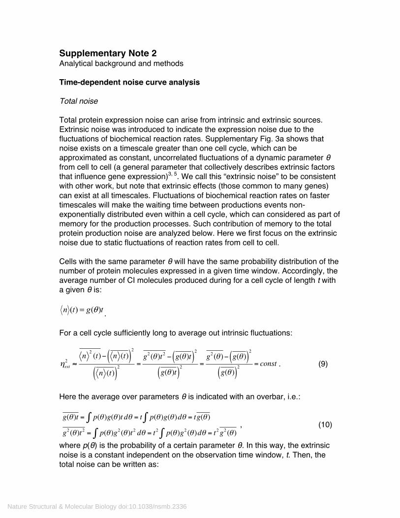
Supplementary Note 2 Analytical background and methods Time-dependent noise curve analysis Total noise Total protein expression noise can arise from intrinsic and extrinsic sources. Extrinsic noise was introduced to indicate the expression noise due to the fluctuations of biochemical reaction rates. Supplementary Fig. 3a shows that noise exists on a timescale greater than one cell cycle, which can be approximated as constant, uncorrelated fluctuations of a dynamic parameter θ from cell to cell (a general parameter that collectively describes extrinsic factors that influence gene expression)3, 5. We call this “extrinsic noise” to be consistent with other work, but note that extrinsic effects (those common to many genes) can exist at all timescales. Fluctuations of biochemical reaction rates on faster timescales will make the waiting time between productions events non-exponentially distributed even within a cell cycle, which can considered as part of memory for the production processes. Such contribution of memory to the total protein production noise are analyzed below. Here we first focus on the extrinsic noise due to static fluctuations of reaction rates from cell to cell. Cells with the same parameter θ will have the same probability distribution of the number of protein molecules expressed in a given time window. Accordingly, the average number of CI molecules produced during for a cell cycle of length t with a given θ is:

tgtn )()( θ= .

For a cell cycle sufficiently long to average out intrinsic fluctuations:

ηext2 ≈

n 2 (t)− n (t)( )2

n (t)( )2 =

g2 (θ )t2 − g(θ )t( )2

g(θ )t( )2 =

g2 (θ )− g(θ )( )2

g(θ )( )2 = const . (9)

Here the average over parameters θ is indicated with an overbar, i.e.:

g(θ )t = p(θ )g(θ )t dθ∫ = t p(θ )g(θ )dθ = t∫ g(θ )

g2 (θ )t2 = p(θ )g2 (θ )t2 dθ∫ = t2 p(θ )g2 (θ )dθ = t2∫ g2 (θ ) , (10)

where p(θ) is the probability of a certain parameter θ. In this way, the extrinsic noise is a constant independent on the observation time window, t. Then, the total noise can be written as:


( )( ) ( )

( )( ) exttot

tn

tntn

tn

tntn

n

ntn2

int2

2

22

2

22

2

222

)(

)()(

)(

)()()(ηηη +=

−⎟⎠⎞⎜⎝

⎛+

⎟⎠⎞⎜⎝

⎛−=

−= . (11)

Thus, the extrinsic noise will contribute a constant term in the total time dependent noise, η2

tot. Correlation and extrinsic noise We first assume that CI production time traces n(θ,t) are dependent on the general parameter θ, and that θ is constant on the time scale of one cell cycle. If a time trace with such a fixed parameter θ is not correlated, n(θ, t)n(θ, t ') = n(θ ) 2 ,

and time traces with different θ are independent on each other, n(θ, t)n(θ ', t ') = n(θ ) n(θ ') ,

then the autocorrelation function of these time traces is: C(t − t ') = d∫ θ p(θ ) n(θ, t)n(θ, t ') − d∫ θ p(θ ) n(θ, t)( )

2

= d∫ θ p(θ ) n(θ ) 2− d∫ θ p(θ ) n(θ, t)( )

2= n(θ ) 2

− n(θ )( )2≠ 0

. (12)

Here, p(θ) is the probability that a generation has a certain parameter θ. This equation shows that the autocorrelation for a process that is memoryless but has extrinsic noise is time independent and will have a non-zero constant value, which is the variance of extrinsic noise. In general, if the process has memory but the parameter θ is still constant on the time scale of one cell cycle:

. The total autocorrelation can be decomposed into two parts:

n(θ, t)n(θ, t ') − n(θ ) 2=Cθ (t − t ') ≠ 0


( )( )

( ) 2'22

222

2

)'()'()()()()'()(

),()()()()()()',(),()(

),()()',(),()()'(

extttCconstttCpdnnttCpd

tnpdnpdnpdtntnpd

tnpdtntnpdttC

σθθθθθθ

θθθθθθθθθθθθθ

θθθθθθθ

θθ +−=+−=−+−=

−+−=

−=−

∫∫∫∫∫∫

∫∫(13)

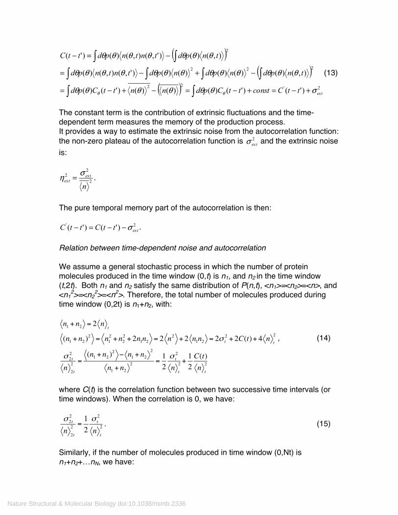
The constant term is the contribution of extrinsic fluctuations and the time-dependent term measures the memory of the production process. It provides a way to estimate the extrinsic noise from the autocorrelation function: the non-zero plateau of the autocorrelation function is 2

extσ and the extrinsic noise is:

2

22

next

extση = .

The pure temporal memory part of the autocorrelation is then:

2' )'()'( extttCttC σ−−=− . Relation between time-dependent noise and autocorrelation We assume a general stochastic process in which the number of protein molecules produced in the time window (0,t) is n1, and n2 in the time window (t,2t). Both n1 and n2 satisfy the same distribution of P(n,t), <n1>=<n2>=<n>, and <n1

2>=<n22>=<n2>. Therefore, the total number of molecules produced during

time window (0,2t) is n1+n2, with: n1 + n2 = 2 n

t

(n1 + n2 )2 = n1

2 + n22 + 2n1n2 = 2 n2 + 2 n1n2 = 2σ t

2 + 2C(t)+ 4 nt

2

σ 2t2

n 2

2t

=(n1 + n2 )

2 − n1 + n22

n1 + n22 =

12σ t2

n 2

t

+12C(t)n 2

t

, (14)

where C(t) is the correlation function between two successive time intervals (or time windows). When the correlation is 0, we have: σ 2t2

n 2

2t

=12σ t2

n 2

t

. (15)

Similarly, if the number of molecules produced in time window (0,Nt) is n1+n2+…nN, we have:


( ) ( ) ( )

)(

)](...)2()2()()1[(21

]...2)2()1[(21

)()(

)]()2()2()()1[(2)(

''2,

2int,

22

'''

2

222

2

2

221

221

221

2

22

222221

21

NtC

nNtNtCtCNtCN

nnn

ntNtCtCNtCN

nn

nnn

nnnnnn

nt

nNtNtCtCNtCNNnnn

nNnnnn

extNtNt

tt

ext

t

extt

Nt

Ntt

t

Nt

N

NN

Nt

NtNt

ttN

tNNt

++=

−++−+−++−=

−++−+−+⋅=

++

++−++==

+−++−+−+=++

=++=

ηη

σσσ

σ

ση

σ

(16)

Eq. 16 shows that the total noise in the number of molecules produced at a particular time window is the sum of the intrinsic noise η2

Nt,int, extrinsic noise η2

Nt,ext, and noise resulting from the correlation C ′′(Nt), which measures the memory effect of the time sequence. When the correlation term and extrinsic noise term are both zero, we have: σ Nt2

n 2

Nt

=1Nσ t2

n 2

t

∝1

N nt

=1n

Nt

. (17)

This is the pure intrinsic noise. When the correlation function is a constant without memory, as the cases of λr3, λb, and λ– in our observations, we have: C(t) ==C(Nt − t) =C

C = n(θ ) 2− n(θ )( )

2

This is the variance of extrinsic noise as in Eq. 12. Therefore, we have:

ηNt2 =

1n

Nt

⋅σ t2

nt

+N(N −1)C

nNt

2 =1n

Nt

⋅ (σ t2 −Cn

t

)+ Cn

t

2 =An

Nt

+B . (18)

Here, A is the intrinsic Fano factor (note the subtraction of the extrinsic Fano factor C/<n>t), and B is the time-independent extrinsic noise. Eq. 18 returns to the commonly seen form where the total noise is simply the sum of intrinsic noise, η2

int, and extrinsic noise, η2ext. Here, the intrinsic noise is inversely

proportional to the mean protein production level for the observation time window


t and extrinsic noise is a constant independent of mean protein production level3,

6. Because the mean protein production level for the observation time window t is proportional to t, η2

int is inversely proportional to t. In Supplementary Figs. 3c and d, we plot the noise curve for strain λr3. The noise curve is well fit by Eq. 18 (same as Eq. 4 in main text) with an intrinsic Fano factor of 2.9 ± 0.1 and extrinsic noise of 0.07 ± 0.01. We note that the noise curve is poorly fit when the extrinsic noise, B, is fixed at zero, or when the intrinsic Fano factor, A, is fixed at 1. In addition, when we restrict the noise analysis to cells having a mean CI production rate within 1.5 or 1 standard deviation of the total population mean, the fitted intrinsic Fano factor A changes little while extrinsic noise B is reduced substantially. This result is consistent with the expectation that intrinsic noise, which is determined by the nature of the biological processes specific to the expression of a specific gene, is unaffected by extrinsic fluctuations; extrinsic noise, a consequence due to static fluctuations in reaction rates from cell to cell, can be reduced by restricting the average protein production range of cells. In our observations, the strain λWT exhibited significant memory (decreasing autocorrelation over a cell cycle). Therefore, the memory term C ′′(Nt) can be calculated as:

22

''''' )](...)2()2()()1[(2)(

tnN

tNtCtCNtCNNtC −++−+−= .

Subtracting C ′′(Nt) from the total noise η2

Nt: η2Nt – C ′′(Nt) is the sum of intrinsic

and extrinsic noise, which can also be fitted by Eq. 18 to obtain the intrinsic Fano factor A and constant extrinsic noise B. The fitting results for all strains: λr3, λb, λ– and λWT are given in Table 1 in the main text. Protein production distribution with the random bursting model Direct observation of expression bursts in a low-expression-level strain To verify whether random, burst-like production of CI could occur at the λ promoter PRM, we examined a low-expression-level strain, λ–

, so that individual bursts may be directly observed. Strain λ– has the same PRM promoter and nearly identical gene sequence compared to that of λr3

, but encodes a short-lived CI by a point mutation. In λ-, there is very little CI because of its shortened lifetime; the Cro protein is expressed and represses PRM (Fig. 2a). The mean production rate of λ– (μ=0.06 ± 0.3, N= 2894 from 217 cells) is much lower than that of λr3, indicating strong repression of PRM by Cro. Consistent with this, we observed small, well-separated expression bursts in λ– (Fig. 2c). The


autocorrelation of λ– is also essentially flat across the time scale examined (Fig. 3a). We counted the number of bursts occurred in a fixed time window and found that the distribution can be described by a Poisson distribution with an average bursting frequency of ~0.6 per cell cycle (Supplementary Fig. 4d). The observation is consistent with the expectation that the waiting time between individual bursts is exponentially distributed. The average burst size (including bursts that do not produce any protein molecules) calculated based on the geometric distribution of burst size is 0.47 ± 0.05. The intrinsic Fano factor and extrinsic noise based on the noise curve analysis are 1.8 ± 0.1 and 0.6 ± 0.3, respectively (Table 1). Master equations We use a simplified random bursting model of gene expression in our noise analysis7-9. In this model, expression events occur randomly with a given rate, g, with each event instantly producing a burst of protein molecules following a geometric size distribution with a mean of n: Gn = q

n (1− q) , so: ddtP(n, t) = g[ GjP(n− j, t)

j=1

n

∑ − qP(n, t)]+ k(n+1)P(n+1, t)− knP(n, t) . (19)

Here, b = q/(1-q) is the average burst size, g is the production frequency, and k is the effective degradation rate. The expected distribution of the concentration of molecules in individual cells has been solved previously8. The concentration distribution is the balanced result of the production and effective degradation (dilution by cell division and degradation). Our experiments monitor the production of protein molecules; hence, we are interested in the distribution of the number of protein molecules produced during a particular observation time window, t. We note that the probability distribution is no longer dependent on the effective degradation processes, but instead depends on the time t: P(n,t). Therefore, in the master equation for the production process we set the effective degradation rate k=0: ddtP(n, t) = g[ GjP(n− j, t)

j=1

n

∑ − qP(n, t)] . (20)

Analytic solution of time-dependent protein production distribution We define the generation function of the production distribution:

0|),(!1),(),(),( ==⇔=∑ zn

n

n

n tzPdzd

ntnPztnPtzP . (21)


The master equations can be converted to one equation for the generation function: ddtP(z, t) = g[q(1− q)zP(z, t)+ q2 (1− q)z2 ++ qn (1− q)znP(z, t)+− qP(z, t)]

= g[(1− q)P(z, t) (qz)n −n=1

∞

∑ qP(z, t)]= g[(1− q)P(z, t) qz1− qz

− qP(z, t)]

= −g (1− q)z1− qz

P(z, t)⇒ P(z, t) = exp −gt (1− z)q1− qz

%

&'

(

)*

. (22)

By defining derivative parameters:

λ = gqt, χ = 1− qq

λ ,

we express the generation function as: P(z, t) = exp[− λ

qz−1z−1/ q

]= exp[− λq]exp[χ 1

1− qz]

= exp[− λq] 1+ χ N 1

(1− qz)NN=1

∞

∑$

%&

'

()

.

We employ the Taylor expansion:

1(1− qz)N

=1+ Nqz+ N(N +1)2!

qz( )2 ++(N )nn!

qz( )n +=(N )nn!

qz( )nn=0

∞

∑

N( )n = N(N +1)(N + n−1).

We derive the Taylor expansion of the generation function:

P(z, t) = exp[− λq] 1+ 1

N!χ N (N )n

n!qz( )n

n=0

∞

∑$

%&

'

()

N=1

∞

∑$

%&&

'

())= P(n, t)zn

n=0

∞

∑

⇒ P(n, t) = exp[− λq] 1

N!χ N (N )n

n!qn

N=1

∞

∑$

%&

'

()= exp[− λ

q] χ N (N + n−1)!

(N −1)!N!n!qn

N=1

∞

∑$

%&

'

()

= exp[− λq] χ N (N + n)!

(N +1)!N!n!N=0

∞

∑$

%&

'

()qnχ

.

The definition of Kummer’s M confluent hypergeometric function is:


∑∑∞

=

∞

= ++=+=+

00 !!)!1()!(

!)2()1(),2,1(

N

N

N N

NN

nNNNn

NnnM χχχ .

We express the production distribution using the Kummer’s function: P(n ≥1, t) = exp[− λ

q]qnχM (n+1,2, χ ) = exp[−gt]qn[(1− q)gt]M[n+1,2, (1− q)gt]

P(n = 0, t) = exp[−gqt]. (23)

It can be checked that this solution satisfies the initial condition: P(0, t = 0) =1,P(n ≠ 0, t = 0) = 0 . Another way to derive the generation function in Eq. 22 and the probability distribution in Eq. 23 is as the total number of molecules produced during a time in which a Poisson-distributed number of bursts occur. For a time window t, the Poisson distribution of the number of burst events nb is:

P(nb, t) =(gt)nb

nb!e−gt .

For each burst, the number of proteins produced follows a geometric distribution. The generation function of a Geometric distribution is: 1− q1− qz

.

Then, the generation function of a Poisson number of geometrically-distributed bursts is:

P(z, t) = (gt)nb

nb!e−gt 1− q

1− qz"

#$

%

&'

nb

nb=0

∞

∑ = e−gtegt 1−q1−qz = exp −gt (1− z)q

1− qz*

+,

-

./ . (24)

This is the same as Eq. 22. Relationship between burst size and intrinsic Fano Factor From the generation function in Eq. 22, we can obtain intrinsic Fano factor for a particular t:


n (t) = ddzP(z, t) |z=1= gt

q1− q

= gbt

n2 (t) = d 2

dz2P(z, t) |z=1 + n (t) = g2 ( q

1− q)2 t2 + 2g( q

1− q)2 t + bgt

= g2b2t2 + 2b2gt + bgt

⇒n2 (t)− n 2 (t)

n 2 (t)=2b2gt + bgtg2b2t2

=2b+1gbt

=2b+1n (t)

. (25).

Therefore, the average burst size, b, is related to the intrinsic Fano factor F by F=2b+1. Burst size in the presence of extrinsic noise Eq. 25 does not consider the influence of extrinsic noise. Extrinsic noise can be treated as fluctuations (ηg and ηb respectively) in the kinetic parameters g and b with distributions p(g) and p(b) respectively5: n (t) = dg dbp(g)p(b)∫∫ gbt = g b t

n2 (t) = dg dbp(g)p(b)∫∫ g2b2t2 + 2b2gt + bgt"# $%= g2 b2 t2 + 2 b2 g t + g b t

⇒n2 (t)− n (t)( )

2

n (t)( )2 =

g2 b2 t2 + 2 b2 g t + g b t − g 2 b 2 t2

g 2 b 2 t2

= (ηb2ηg

2 +ηg2 +ηb

2 )+2 b2 g + g b

g 2 b 21t= (ηb

2ηg2 +ηg

2 +ηb2 )+

2(ηb2 +1) b +1n (t) (26)

Here, the total noise is decomposed into intrinsic and extrinsic parts:

η2int =2(ηb

2 +1) b +1n (t)

and η2ext = (ηb2ηg

2 +ηg2 +ηb

2 ) . (27)

Therefore, in the presence of extrinsic noise, the measured intrinsic Fano factor, F, is related to the average burst size b by:

1)1(2 2 ++= bF bη . (28) To estimate how much the average burst size is influenced by extrinsic noise, we assume an extreme condition where all the extrinsic noise comes from the fluctuation in burst size ηb. Because extrinsic noise of λr3, λb and λWT is less then


0.1, the maximal value of ηb2 will then be ~0.1. Therefore, extrinsic noise would

change the average burst size by 10% at most. However, in the case of λ–, where the extrinsic noise is ~0.6 the burst size of λ– will then be between 0.25 and 0.40. The geometric burst model is a special case for a memoryless system whose noise curve can be decomposed into intrinsic and extrinsic parts; as shown in Eq. 18:

η2tot (t) =η2int (t)+η

2ext (t) =

An

Nt

+B , with A = 2(ηb2 +1) b +1,B = (ηb

2ηg2 +ηg

2 +ηb2 ) . (29)

Derivation of protein burst size from transcriptional and translational burst sizes Consider a two-step bursting process in which a geometrically distributed transcriptional burst produces an average of b1 = q1/(1-q1) mRNA molecules per burst, and each mRNA molecule produces a geometrically distributed number of proteins with an average burst size b2 = q2/(1-q2). Since the mRNA lifetime is usually short in bacterial cells and our autocorrelation results imply that the protein production process is essentially memoryless, we assume that these two bursts happen close in time so that the waiting time between them is negligibly short. Thus, using the generation function of Geometric distribution: (1-q)/(1-qz), the effective geometric burst distribution of these two instant burst has the generation function:

(1− q1) q1n (1− q2 )

n

(1− q2z)n

n∑ =

1

1− q11− q21− q2z

=1− q2z

1− q1 − q2z+ q1q2

=1

1− q1 − q2z+ q1q2− q2z

11− q1 − q2z+ q1q2

. (30)

Expanding in order of z, we get the effective burst size distribution Gj:

Gj≥1 = 1− q1( ) 11− q1 + q1q2

q21− q1 + q1q2

#

$%

&

'(

j

− q21

1− q1 + q1q2q2

1− q1 + q1q2

#

$%

&

'(

j−1)

*++

,

-..

= 1− q1( ) q1(1− q2 )1− q1 + q1q2

q21− q1 + q1q2

#

$%

&

'(

j

= q1(1−Q)Qj

Gj=0 =1− q1

1− q1 + q1q2=1− q1Q

, (31)

with:


211

2

1 qqqqQ+−

= .

This is a geometric distribution for j ≥1 . Furthermore, the effective master equations can be rewritten as:

),(),1()1()],(),('[

),(),1()1()],(),('[),(

11

111

tnknPtnPnktnQPtjnPGgq

tnknPtnPnktnQPqtjnPGqgtnPdtd

n

jj

n

jj

−+++−−=

−+++−−=

∑

∑

=

= . (32)

There is a new burst frequency 1gq , a new geometric distribution )1(' QQG j

j −= for j ≥ 0 and a new average burst size:

2121

2 )1()1)(1(1

bbqq

qQQB +=

−−=

−= . (33)

Eq. 32 shows that by modifying the bursting frequency g to gq1, the effective burst size distribution for sequential geometrically distributed bursts with no time interval between them is still a geometric distribution, and the average burst size can be calculated according to Eq. 33. In Eq. 25, we show that for the random burst model the intrinsic Fano factor, A, is related to the average burst size, b, by 12 +≈ bA . Using this equation and the intrinsic Fano factor obtained from noise curve analysis, we calculated burst sizes of 0.40 ± 0.06 and 0.95 ± 0.04 for λ– and λr3, respectively. The random bursting model does not distinguish translational bursting from transcriptional bursting as long as the final protein burst size follows a geometric distribution. Assuming that there are geometric transcriptional and translational bursts with average burst sizes of b1 and b2 respectively, in Eq. 33, we show that the combined process can still be treated as a single bursting step with a final geometric protein burst size 21)1( bbb += . Because the transcripts in λ– and λr3 are essentially identical in sequence, we assume that the average translational burst size b2 is identical for both strains. Therefore, we obtain the average transcriptional burst size of λr3:

−−− +≈−+= 11

331 4.24.11)1( bb

bbbr

r ,

where −1b is the transcriptional burst size of λ–. If transcription in λ– is Poissonian

(e.g. −1b =0, a reasonable assumption for a strongly repressed promoter10), the

average transcriptional burst size of λr3 will still be greater than zero, suggesting the presence of transcriptional bursting in λr3.


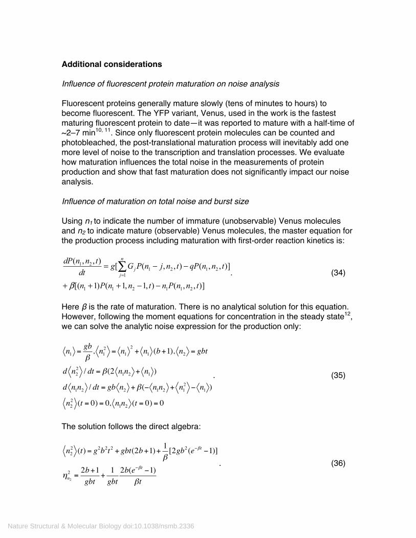
Additional considerations Influence of fluorescent protein maturation on noise analysis Fluorescent proteins generally mature slowly (tens of minutes to hours) to become fluorescent. The YFP variant, Venus, used in the work is the fastest maturing fluorescent protein to date—it was reported to mature with a half-time of ~2–7 min10, 11. Since only fluorescent protein molecules can be counted and photobleached, the post-translational maturation process will inevitably add one more level of noise to the transcription and translation processes. We evaluate how maturation influences the total noise in the measurements of protein production and show that fast maturation does not significantly impact our noise analysis. Influence of maturation on total noise and burst size Using n1 to indicate the number of immature (unobservable) Venus molecules and n2 to indicate mature (observable) Venus molecules, the master equation for the production process including maturation with first-order reaction kinetics is:

)],,(),1,1()1[(

)],,(),,([),,(

211211

211

2121

tnnPntnnPn

tnnqPtnjnPGgdt

tnndP n

jj

−−+++

−−= ∑=

β. (34)

Here β is the rate of maturation. There is no analytical solution for this equation. However, following the moment equations for concentration in the steady state12, we can solve the analytic noise expression for the production only:

n1 =gbβ, n1

2 = n12+ n1 (b+1), n2 = gbt

d n22 / dt = β(2 n1n2 + n1 )

d n1n2 / dt = gb n2 +β(− n1n2 + n12 − n1 )

n22 (t = 0) = 0, n1n2 (t = 0) = 0

. (35)

The solution follows the direct algebra: n22 (t) = g2b2t2 + gbt(2b+1)+ 1

β[2gb2 (e−βt −1)]

ηn22 =

2b+1gbt

+1gbt

2b(e−βt −1)βt

. (36)


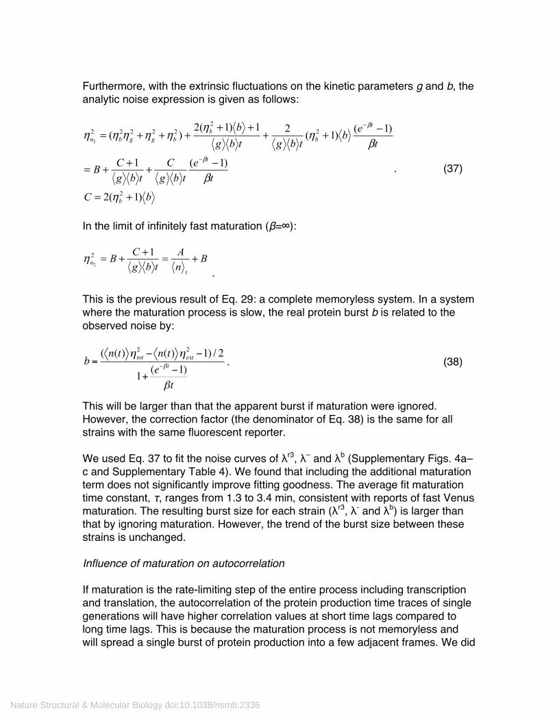
Furthermore, with the extrinsic fluctuations on the kinetic parameters g and b, the analytic noise expression is given as follows:

bC

te

tbgC

tbgCB

teb

tbgtbgb

b

t

t

bb

bggbn

)1(2

)1(1

)1()1(21)1(2)(

2

22

222222

+=

−+++=

−++++

+++=

−

−

η

β

βη

ηηηηηη

β

β

. (37)

In the limit of infinitely fast maturation (β=∞):

. This is the previous result of Eq. 29: a complete memoryless system. In a system where the maturation process is slow, the real protein burst b is related to the observed noise by:

b =( n(t) η2tot − n(t) η2ext −1) / 2

1+ (e−βt −1)βt

. (38)

This will be larger than that the apparent burst if maturation were ignored. However, the correction factor (the denominator of Eq. 38) is the same for all strains with the same fluorescent reporter. We used Eq. 37 to fit the noise curves of λr3, λ– and λb (Supplementary Figs. 4a–c and Supplementary Table 4). We found that including the additional maturation term does not significantly improve fitting goodness. The average fit maturation time constant, τ, ranges from 1.3 to 3.4 min, consistent with reports of fast Venus maturation. The resulting burst size for each strain (λr3, λ- and λb) is larger than that by ignoring maturation. However, the trend of the burst size between these strains is unchanged. Influence of maturation on autocorrelation If maturation is the rate-limiting step of the entire process including transcription and translation, the autocorrelation of the protein production time traces of single generations will have higher correlation values at short time lags compared to long time lags. This is because the maturation process is not memoryless and will spread a single burst of protein production into a few adjacent frames. We did

BnA

tbgCB

tn +=++= 122

η


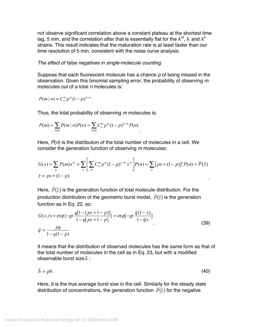
not observe significant correlation above a constant plateau at the shortest time lag, 5 min, and the correlation after that is essentially flat for the λr3, λ- and λb strains. This result indicates that the maturation rate is at least faster than our time resolution of 5 min, consistent with the noise curve analysis. The effect of false negatives in single-molecule counting Suppose that each fluorescent molecule has a chance p of being missed in the observation. Given this binomial sampling error, the probability of observing m molecules out of a total n molecules is:

. Thus, the total probability of observing m molecules is:

. Here, P(n) is the distribution of the total number of molecules in a cell. We consider the generation function of observing m molecules:

. Here, ( )zP is the generation function of total molecule distribution. For the production distribution of the geometric burst model, ( )zP is the generation function as in Eq. 22, so:

)1(1

]1

)1(exp[}]1[1)]1(1[exp{),(

pqpqq

xqxqgt

ppxqppxqgttxG

−−=

−−−=

−+−−+−−=

. (39)

It means that the distribution of observed molecules has the same form as that of the total number of molecules in the cell as in Eq. 23, but with a modified observable burst sizeb :

pbb = . (40) Here, b is the true average burst size in the cell. Similarly for the steady state distribution of concentrations, the generation function ( )zP for the negative

mnmmn ppCnmP −−= )1()|(

∑∑≥

−

≥

−==mn

mnmmn

mnnPppCnPnmPmP )()1()()|()(

)1(

)()()]1([)()1()()(

ppxz

zPnPppxnPxppCxmPxGn

n

n m

mmnmmn

m

m

−+=

=−+=⎥⎦⎤

⎢⎣⎡ −== ∑∑ ∑∑ −


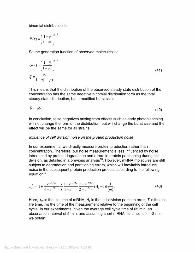
binomial distribution is:

kg

zqqzP

/

11)( ⎟⎟⎠

⎞⎜⎜⎝

⎛−−= .

So the generation function of observed molecules is:

)1(1

11)(

/

pqpqq

xqqxG

kg

−−=

⎟⎟⎠

⎞⎜⎜⎝

⎛−−=

. (41)

This means that the distribution of the observed steady state distribution of the concentration has the same negative binomial distribution form as the total steady state distribution, but a modified burst size:

. (42) In conclusion, false negatives arising from effects such as early photobleaching will not change the form of the distribution, but will change the burst size and the effect will be the same for all strains. Influence of cell division noise on the protein production noise In our experiments, we directly measure protein production rather than concentration. Therefore, our noise measurement is less influenced by noise introduced by protein degradation and errors in protein partitioning during cell division, as detailed in a previous analysis13. However, mRNA molecules are still subject to degradation and partitioning errors, which will inevitably introduce noise in the subsequent protein production process according to the following equation13:

mA

ee

ee

Tt

ee

yT

t

t

T

T

t

m m

m

m

m

m

m 1)]1(22

11

41[ /

/

/

/

/2

/22 −

−−

−−

−+= −

−

−

−

−

−

τ

τ

τ

τ

τ

τ

η . (43)

Here, τm is the life time of mRNA, Ay is the cell division partition error, T is the cell life time, t is the time of the measurement relative to the beginning of the cell cycle. In our experiments, given the average cell cycle time of 65 min, an observation interval of 5 min, and assuming short mRNA life time, τm ~1–2 min, we obtain:

pbb =


mm12 ≈η . (44)

This indicates that for mRNA molecules having short life times, the noise in mRNA copy number distribution won’t be significantly affected by the cell division partition error. Therefore, partitioning error at cell division should have minimal effect on protein production noise.


Supplementary Movie 1 Timelapse fluorescence images (spots pseudo-colored yellow to indicate the production of Tsr-Venus-Ub molecules) overlaid with corresponding bright field images of E. coli colonies grown in a temperature-controlled chamber on a microscope stage at 37° C for strain λWT. Images were acquired every 5 min. Scale bar depicts 5 μm. Images generated in ImageJ by subtracting 6th fluorescent image from 1st image for each timepoint (Supplementary Fig. 1c). Each subtraction image was bandpass filtered, linearly scaled to enhance contrast, and used to generate a yellow image that was added to the bright field image from the same time point (shown at very low contrast so that cell outlines and pole-localized Venus molecules are both visible). The same maximum and minimum intensities were used to scale fluorescence images for λWT, λr3 (Supplementary Movie 2) and λb (Supplementary Movie 3) movies. Higher contrast was used for the λ– (Supplementary Movie 4) movie because of its much lower expression level. Supplementary Movie 2 Timelapse fluorescence images for strain λr3. Methods detailed in Supplementary Movie 1 legend. Supplementary Movie 3 Timelapse fluorescence images for strain λb. Methods detailed in Supplementary Movie 1 legend. Supplementary Movie 4 Timelapse fluorescence images for strain λ–. Methods detailed in Supplementary Movie 1 legend.


Supplementary References 1. Rosenfeld, N., et al., Gene regulation at the single-cell level. Science.

307(5717): p. 1962-5. (2005) 2. So, L.H., et al., General properties of transcriptional time series in

Escherichia coli. Nat Genet. 43(6): p. 554-60. (2011) 3. Swain, P.S., Elowitz, M.B., and Siggia, E.D., Intrinsic and extrinsic

contributions to stochasticity in gene expression. Proc Natl Acad Sci USA. 99(20): p. 12795-800. (2002)

4. Elowitz, M.B., et al., Stochastic gene expression in a single cell. Science. 297(5584): p. 1183-6. (2002)

5. Taniguchi, Y., et al., Quantifying E. coli proteome and transcriptome with single-molecule sensitivity in single cells. Science. 329(5991): p. 533-8. (2010)

6. Paulsson, J., Summing up the noise in gene networks. Nature. 427(6973): p. 415-8. (2004)

7. Paulsson, J., Berg, O.G., and Ehrenberg, M., Stochastic focusing: fluctuation-enhanced sensitivity of intracellular regulation. Proc Natl Acad Sci USA. 97(13): p. 7148-53. (2000)

8. Paulsson, J. and Ehrenberg, M., Random signal fluctuations can reduce random fluctuations in regulated components of chemical regulatory networks. Phys Rev Lett. 84(23): p. 5447-50. (2000)

9. Paulsson, J. and Ehrenberg, M., Noise in a minimal regulatory network: plasmid copy number control. Q Rev Biophys. 34(1): p. 1-59. (2001)

10. Yu, J., et al., Probing gene expression in live cells, one protein molecule at a time. Science. 311(5767): p. 1600-3. (2006)

11. Nagai, T., et al., A variant of yellow fluorescent protein with fast and efficient maturation for cell-biological applications. Nat Biotechnol. 20(1): p. 87-90. (2002)

12. Pedraza, J.M. and Paulsson, J., Effects of molecular memory and bursting on fluctuations in gene expression. Science. 319(5861): p. 339-43. (2008)

13. Huh, D. and Paulsson, J., Non-genetic heterogeneity from stochastic partitioning at cell division. Nat Genet. 43(2): p. 95-100. (2010)


Online Supplementary Material Stochastic expression ... · Online Supplementary Material Stochastic...

Documents

Transcript of Online Supplementary Material Stochastic expression ... · Online Supplementary Material Stochastic...