SANDIA REPORTSAND2016-9282Unlimited ReleasePrinted September 2016

Online Mapping and Forecasting ofEpidemics Using Open-Source Indicators

J. Ray, S. Lefantzi, J. Bauer, M. Khalil, A. Rothfuss, K. R. Cauthen, P. D. Finley and H. Smith

Prepared bySandia National LaboratoriesAlbuquerque, New Mexico 87185 and Livermore, California 94550

Sandia National Laboratories is a multi-program laboratory managed and operated by Sandia Corporation,a wholly owned subsidiary of Lockheed Martin Corporation, for the U.S. Department of Energy’sNational Nuclear Security Administration under contract DE-AC04-94AL85000.

Approved for public release; further dissemination unlimited.

Issued by Sandia National Laboratories, operated for the United States Department of Energyby Sandia Corporation.

NOTICE: This report was prepared as an account of work sponsored by an agency of the UnitedStates Government. Neither the United States Government, nor any agency thereof, nor anyof their employees, nor any of their contractors, subcontractors, or their employees, make anywarranty, express or implied, or assume any legal liability or responsibility for the accuracy,completeness, or usefulness of any information, apparatus, product, or process disclosed, or rep-resent that its use would not infringe privately owned rights. Reference herein to any specificcommercial product, process, or service by trade name, trademark, manufacturer, or otherwise,does not necessarily constitute or imply its endorsement, recommendation, or favoring by theUnited States Government, any agency thereof, or any of their contractors or subcontractors.The views and opinions expressed herein do not necessarily state or reflect those of the UnitedStates Government, any agency thereof, or any of their contractors.

Printed in the United States of America. This report has been reproduced directly from the bestavailable copy.

Available to DOE and DOE contractors fromU.S. Department of EnergyOffice of Scientific and Technical InformationP.O. Box 62Oak Ridge, TN 37831

Telephone: (865) 576-8401Facsimile: (865) 576-5728E-Mail: reports@adonis.osti.govOnline ordering: http://www.osti.gov/bridge

Available to the public fromU.S. Department of CommerceNational Technical Information Service5285 Port Royal RdSpringfield, VA 22161

Telephone: (800) 553-6847Facsimile: (703) 605-6900E-Mail: orders@ntis.fedworld.govOnline ordering: http://www.ntis.gov/help/ordermethods.asp?loc=7-4-0#online

DEP

ARTMENT OF ENERGY

• • UN

ITED

STATES OF AM

ERI C

A

2

SAND2016-9282Unlimited Release

Printed September 2016

Online Mapping and Forecasting of Epidemics Using Open-SourceIndicators

J. Ray, S. Lefantzi, J. Bauer, M. Khalil, A. RothfussSandia National Laboratories, P. O. Box 969, Livermore CA 94551

K. R. Cauthen, P. D. Finley, H. SmithSandia National Laboratories, P. O. Box 5800, Albuquerque NM 87185-0751

G. LambertApple Inc, 1 Results Way, Cupertino, CA 95014

{jairay,slefant,josbaue,mkhalil,arothfu,kcauthe,pdfinley,hsmith}@sandia.gov,gregory lambert@apple.com

Abstract

Open-source indicators have been proposed as a way of tracking and forecasting disease outbreaks. Some,such are meteorological data, are readily available as reanalysis products. Others, such as those derived fromour online behavior (web searches, media article etc.) are gathered easily and are more timely than publichealth reporting. In this study we investigate how these datastreams may be combined to provide usefulepidemiological information. The investigation is performed by building data assimilation systems to trackinfluenza in California and dengue in India. The first does not suffer from incomplete data and was chosento explore disease modeling needs. The second explores the case when observational data is sparse anddisease modeling complexities are beside the point. The two test cases are for opposite ends of the diseasetracking spectrum.

We find that data assimilation systems that produce disease activity maps can be constructed. Further, beingable to combine multiple open-source datastreams is a necessity as any one individually is not very infor-mative. The data assimilation systems have very little in common except that they contain disease models,calibration algorithms and some ability to impute missing data. Thus while the data assimilation systemsshare the goal for accurate forecasting, they are practically designed to compensate for the shortcomings ofthe datastreams. Thus we expect them to be disease and location-specific.

3

Acknowledgment

This work was funded under LDRD (Laboratory Directed Research and Development) Project Number173112 and Title “Online Mapping and Forecasting of Epidemics Using Open-Source Indicators”. SandiaNational Laboratories is a multi-program laboratory managed and operated by Sandia Corporation, a whollyowned subsidiary of Lockheed Martin Corporation, for the U.S. Department of Energy’s National NuclearSecurity Administration under contract DE-AC04-94AL85000.

4

Contents

1 Motivation, hypothesis and tests 9

2 Data assimilation for influenza 11

2.1 Introduction . . . . . . . . . . . . . . . . . . . . . . . . . . . . . . . . . . . . . . . . . . . . . . . . . . . . . . . . . . . . . . . . 11

2.2 Materials and Methods . . . . . . . . . . . . . . . . . . . . . . . . . . . . . . . . . . . . . . . . . . . . . . . . . . . . . . . . 13

2.2.1 Data . . . . . . . . . . . . . . . . . . . . . . . . . . . . . . . . . . . . . . . . . . . . . . . . . . . . . . . . . . . . . . . . 13

2.2.2 Temporal Prediction . . . . . . . . . . . . . . . . . . . . . . . . . . . . . . . . . . . . . . . . . . . . . . . . . . . 13

2.2.3 Spatial Prediction . . . . . . . . . . . . . . . . . . . . . . . . . . . . . . . . . . . . . . . . . . . . . . . . . . . . . 15

2.3 Results . . . . . . . . . . . . . . . . . . . . . . . . . . . . . . . . . . . . . . . . . . . . . . . . . . . . . . . . . . . . . . . . . . . . 17

2.4 Conclusions . . . . . . . . . . . . . . . . . . . . . . . . . . . . . . . . . . . . . . . . . . . . . . . . . . . . . . . . . . . . . . . . 19

3 Data assimilation for dengue 25

3.1 Introduction . . . . . . . . . . . . . . . . . . . . . . . . . . . . . . . . . . . . . . . . . . . . . . . . . . . . . . . . . . . . . . . . 25

3.2 Materials and methods . . . . . . . . . . . . . . . . . . . . . . . . . . . . . . . . . . . . . . . . . . . . . . . . . . . . . . . . 26

3.2.1 Data . . . . . . . . . . . . . . . . . . . . . . . . . . . . . . . . . . . . . . . . . . . . . . . . . . . . . . . . . . . . . . . . 26

3.2.2 Conditionally auto-regressive models . . . . . . . . . . . . . . . . . . . . . . . . . . . . . . . . . . . . . . 27

3.2.3 Boosting . . . . . . . . . . . . . . . . . . . . . . . . . . . . . . . . . . . . . . . . . . . . . . . . . . . . . . . . . . . . 28

3.3 Results . . . . . . . . . . . . . . . . . . . . . . . . . . . . . . . . . . . . . . . . . . . . . . . . . . . . . . . . . . . . . . . . . . . . 28

3.4 Conclusions . . . . . . . . . . . . . . . . . . . . . . . . . . . . . . . . . . . . . . . . . . . . . . . . . . . . . . . . . . . . . . . . 29

4 Follow-on applications 33

4.1 Data assimilation for wildfires . . . . . . . . . . . . . . . . . . . . . . . . . . . . . . . . . . . . . . . . . . . . . . . . . . 33

4.2 Data assimilation and disease modeling . . . . . . . . . . . . . . . . . . . . . . . . . . . . . . . . . . . . . . . . . . 35

5 Conclusions 37

5

References . . . . . . . . . . . . . . . . . . . . . . . . . . . . . . . . . . . . . . . . . . . . . . . . . . . . . . . . . . . . . . . . . . . . . . 39

6

List of Figures

2.1 Data assimilation for San Francisco for 2014-2015 influenza season, starting September 21,2014. At the very top, we plot V (o) (symbols) and V ; the data is available every week. In thesecond plot, we illustrate the inferred evolution of I(t). The third plot shows the estimateof β(t) and the plot at the very bottom shows the convergence of the value of τ over timemeasured in days. . . . . . . . . . . . . . . . . . . . . . . . . . . . . . . . . . . . . . . . . . . . . . . . . . . . . . . . . . . . . 16

2.2 One week ahead forecasts of GFT data for San Francisco during the 2014-2015 influenzaseason. The line is the mean forecast and the error bars the ±3ς predictive uncertaintybounds. The symbols are the GFT data used in the joint state and parameter estimationproblem. . . . . . . . . . . . . . . . . . . . . . . . . . . . . . . . . . . . . . . . . . . . . . . . . . . . . . . . . . . . . . . . . . . . 17

2.3 Left: Error between Y (o) and Y , the modeled forecast value of ILI+, normalized by Y (o)

i.e., η = (Y −Y (o))/Y (o). Here Y is the week-ahead mean forecast. The horizontal solidgreen lines are the ±10% error bounds. Each symbol denotes one of the 11 Californiancities tracked by GFT. Right: The same test of forecasting accuracy, but Y is the two-week-ahead predictions. Results are for the 2014-2015 influenza season. The start and end of theinfluenza season in California is denoted by the dashed blue line, and spans January to March. 18

2.4 Left: Error between Y (o) and Y , the modeled forecast value of ILI+, normalized by 3ς. HereY is the week ahead forecast. The horizontal solid green lines are show whether the observeddata fall within the 99% credibility interval. Each symbol denotes one of the 11 Californiancities tracked by GFT. Right: The same test of forecasting accuracy, but performed for two-week-ahead predictions. Results are for the 2014-2015 influenza season. The start and endof the influenza season in California is denoted by the dashed blue line, and spans Januaryto March. . . . . . . . . . . . . . . . . . . . . . . . . . . . . . . . . . . . . . . . . . . . . . . . . . . . . . . . . . . . . . . . . . . 19

2.5 Nowcast ILI+ intensity map, computed using the spatial prediction method described inSec. 2.2.3. . . . . . . . . . . . . . . . . . . . . . . . . . . . . . . . . . . . . . . . . . . . . . . . . . . . . . . . . . . . . . . . . . . 20

2.6 Test of accuracy of the spatial prediction described in Sec. 2.2.3. On the left, we nowcastILI+ activity in San Mateo County in the San Francisco Bay Area (solid black line) usingILI+ data from nearby municipalities (dashed lines). On the right, we perform a spatiotem-poral forecast, using one-week-ahead forecasts of ILI+ activity of nearby municipalities.Vertical green lines show the approximate start and end of the intense influenza activity in2013-2014. . . . . . . . . . . . . . . . . . . . . . . . . . . . . . . . . . . . . . . . . . . . . . . . . . . . . . . . . . . . . . . . . 21

2.7 ILI+ intensity maps developed for the last week of March 2015. Left: A nowcast. Right: Aone-week-ahead forecast. . . . . . . . . . . . . . . . . . . . . . . . . . . . . . . . . . . . . . . . . . . . . . . . . . . . . . . 21

2.8 A snapshot of the output of the data assimilation system, displayed as a web page on aninternal Sandia server. . . . . . . . . . . . . . . . . . . . . . . . . . . . . . . . . . . . . . . . . . . . . . . . . . . . . . . . . 22

7

3.1 Plots of the binned counts of HM articles on dengue for India for October 2011 (left), 2012(middle) and 2013 (right). The blank states recorded no data. States with data are shadedwith a color corresponding to the lower bound of their bin. We see missing data occurs atrandom. . . . . . . . . . . . . . . . . . . . . . . . . . . . . . . . . . . . . . . . . . . . . . . . . . . . . . . . . . . . . . . . . . . . 27

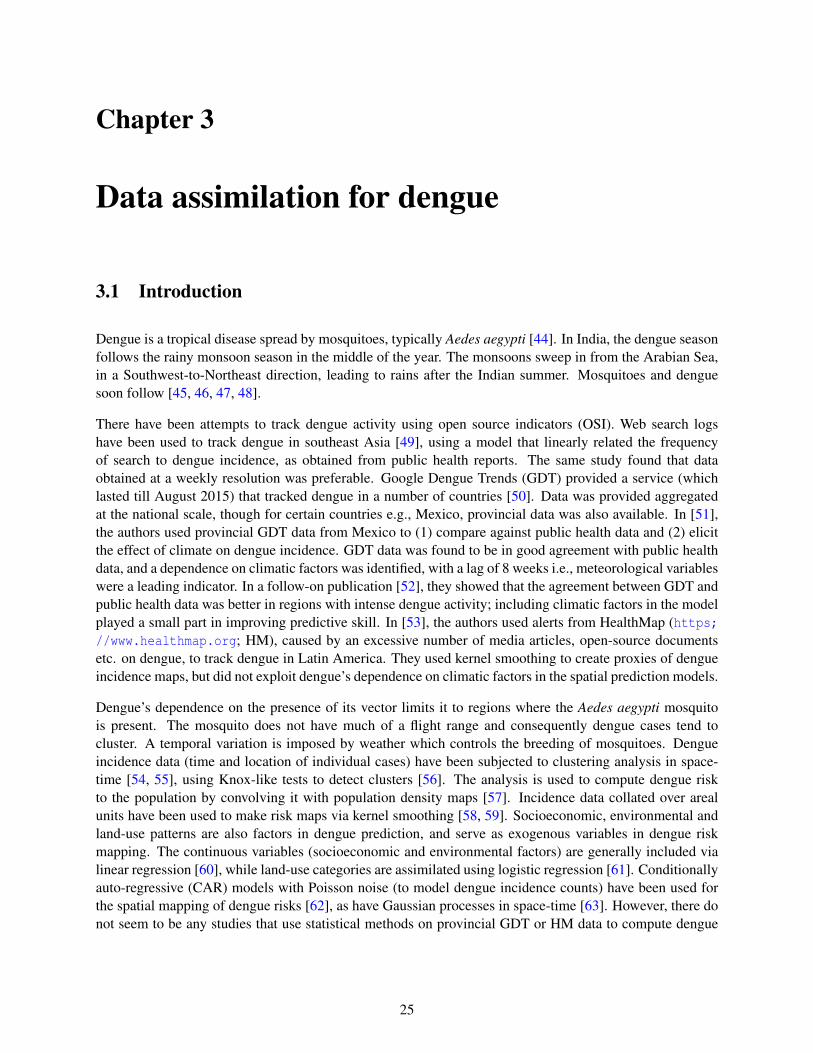
3.2 A comparison of the predictive error for the boosted (red) and non-boosted STCAR forfilling in missing data. Results are plotted for the 15 states where there is some HM data.Overall boosting improves performance . . . . . . . . . . . . . . . . . . . . . . . . . . . . . . . . . . . . . . . . . . 29

3.3 Top: The raw HealthMap data with gaps in it. Bottom: Filled in version of the HealthMapdataset. . . . . . . . . . . . . . . . . . . . . . . . . . . . . . . . . . . . . . . . . . . . . . . . . . . . . . . . . . . . . . . . . . . . . 30

3.4 Left: Forecast of the HM data, for the state of Kerala. The blue dot is the mean prediction,with the shaded error being the 90% and 99% credibility intervals. The red dot is the true(not filled in) value. Right: The same, but for the state of Maharashtra. . . . . . . . . . . . . . . . . . . 31

4.1 The wildfire after two hours. No observational data have been assimilated. The spread inforecast fire fronts (red contours) are due to our ignorance of wind and initial conditions.The blue contour is the true fire front. . . . . . . . . . . . . . . . . . . . . . . . . . . . . . . . . . . . . . . . . . . . . 34

4.2 The wildfire after five hours. Data assimilation has occurred and reduces the uncertaintyspread. The snapshot shows results displayed in SUMMIT’s web client. The red contoursare the 5 hour forecasts without data assimilation. A very narrow ensemble of purple firefronts, very near the blue (true) fire front (and difficult to see) is the forecast ensemble, afterassimilating data available after two hours. . . . . . . . . . . . . . . . . . . . . . . . . . . . . . . . . . . . . . . . 35

4.3 The wildfire after five hours, in detail. The uncertainty spreads show risk to human habita-tion and reinforce the need for data assimilation and probabilistic forecasting using filteringmethods. The purple ensemble is easy to see and shows the enormous decrease in forecast-ing uncertainty effected by the assimilation of data after two hours. . . . . . . . . . . . . . . . . . . . . . 36

8

Chapter 1

Motivation, hypothesis and tests

Fast, dependable forecasting of disease activity can revolutionize medical planning and response. Collectionof public health (PH) data, traditionally used for this purpose, is slow and thus not useful for effectiveresponse. Due to its voluntary nature, epidemiological reporting typically has irregular and incompletespatial coverage. Thus, real- time mapping and forecasting of epidemiological activity is still not feasible.

Online, open-source indicators (OSI) of disease activity e.g., disease-related searches, media reports etc. andmeteorology can serve as strong covariates and leading indicators of outbreaks. They are readily available,timely, and have far superior spatiotemporal resolution than PH data, especially in developing countries.Currently there are few data assimilation (DA) methods that can fuse disparate datastreams to compensatefor delayed/unavailable PH data, nor meteorology-driven disease models for accurate spatiotemporal fore-casting. We propose to develop the methods and models and integrate them into a DA framework. Such aframework would be invaluable for disease tracking in the US and globally.

The key hypothesis behind this study is that OSI are sufficiently rich to calibrate a high-resolution spatialrepresentation of disease activity, modeled on weather patterns. Within the DA framework, the spatialmodel will interpolate sparse disease data. OSI are noisy datastreams, and the spatial model will allownoise suppression by pooling of information across monitored sites (generally large cities). The spatialmodel, along with the meteorology-driven disease model, will allow OSI-calibrated forecasts in regionsoutside OSI coverage. Scalable ensemble Kalman filters will provide the mathematical underpinnings ofdata fusion so that the framework can be applied to country-sized problems. The game-changing potentialof data assimilation has not been applied to disease forecasting, because it has relied on sparse PH data.OSI, and our data assimilation framework, would be a novel development with impact in data- poor regions.

We will demonstrate this via a three step process. First, we will develop a data assimilation system toperform spatiotemporal forecasting of influenza in California, where data is plentiful. Next we will developa system for tracking the evolution of the annual dengue outbreak in India using OSI data from HealthMap(https://www.healthmap.org). This second effort is expected to raise data issues (e.g., missing data)which are not expected in case of Californian influenza. We conclude with a test of generality. We showhow the algorithms and capabilities developed during the construction of the data assimilation systems canbe leveraged in other problems, especially where the data worth of open-source data streams (or the modelsthat ingest them) have to be assessed.

9

10

Chapter 2

Data assimilation for influenza

2.1 Introduction

Seasonal influenza results in between a quarter to half a million deaths worldwide every year, with 3-5 mil-lion cases of severe illness [1]. Many countries have influenza surveillance networks of sentinel physicianswho track cases of influenza-like illness (ILI, defined as a fever over 37.8oC plus cough and/or sore throat;patients for whom the etiology is known not to be influenza are not classified as ILI) ; for example, UnitedStates’ Center for Disease Control (CDC) Outpatient Influenza-like Illness Surveillance Network (ILINet)consists of a group of 2900 outpatient healthcare professionals who voluntarily provide information on totaland ILI-related visits that they receive. The data is compiled, processed and publicly reported on a weeklybasis [2], with a 1-2 week delay [3]. Note that since ILI symptoms can be caused by a number of diseasesother than influenza e.g., rhinovirus and respiratory syncytial virus, CDC also reports data on laboratorysamples testing positive for influenza at the national and regional levels [4]. Note also that many coun-tries and indeed, many counties in the United States itself, do not have such a comprehensive influenzasurveillance infrastructure.

Epidemiological outbreaks leave an imprint on our online lives as we search for information on the disease.Consequently, there have been attempts to track disease activity using web search query logs [3, 5], Twitterposts [6, 7], Wikipedia article views [8, 9] and clinician and medical databases [10]. In most cases, theunderlying hypothesis in these digital disease detection (DDD) techniques is that the intensity of diseaseactivity is correlated with the intensity of the activity in diverse digital datastreams. Statistical models havebeen devised to relate ILINet data (taken as the ground truth of ILI activity) to the easily observed digitalproxies. Since these digital proxies are timely, they are used to “nowcast” the current influenza/ILI activitylevel, 1-2 weeks ahead of the release of ILINet data.

Google Flu Trends (GFT; [3]) is one of the oldest and better known DDD efforts to track ILI. Originally,it used a set of 45 keywords to determine if a Google search was related to ILI and gathered a time-seriesof the volume of ILI-related searches. This time-series was found to be correlated to ILINet data. A modelwas built by regressing ILINet data to a normalized version of the web search time-series. The method wasdependent on the choice of keywords whose usage could evolve with time; consequently, GFT has oftenbeen wrong in its nowcasts [11, 12]. It has been revised a few times [13, 14] and was discontinued in mid-2015. The revisions were mainly about changing/extending the set of keywords used to pick ILI-related websearches. There have been attempts to improve on this basic method - in [15, 16] the authors hypothesizedthat the picking power of diverse keywords was variable (and also changed over time) and determinedweights for various keywords by regressing ILINet data to time-series of web search queries picked by eachof the keywords. They used shrinkage regression to eliminate keywords with negligible predictive powerand performed this calibration for different time periods. They also released the set of keywords. Other

11

studies have hypothesized that DDD datastreams (GFT, medical databases, microblog posts etc.) are weakpredictors of ILI activity but could be combined, in a weighted manner, to increase their predictive power;studies that do so in a variety of ways can be found in [17, 18, 19].

One need not depend on digital proxies for forecasting influenza activity - Tamerius et al [20] showedthat relative humidity and temperature were good predictors of influenza activity, though their effect wasmuted in the tropics. Soebiyanto et al [21] modeled influenza activity in Hong Kong, using precipitation,temperature and relative humidity as the predictors. In [22, 23], the authors used a SIRS (susceptible-infected-recovered-susceptible) model of influenza, with an absolute humidity-based basic reproductionnumber, to forecast influenza (not ILI) activity in approximately 100 US municipalities using GFT data.They used an ensemble adjustment Kalman filter to calibrate the humidity-dependent SIRS model to GFTdata, modified (using ILINet’s data on laboratory samples testing positive for influenza) to reflect influenza,not ILI activity (see [24] for a description). They produced 1-4 week-ahead forecasts. Cities on the USEast Coast were predicted better than West Coast municipalities. The Bayesian nature of the assimilationallowed them to also estimate various disease characteristics e.g., incubation period, and produce forecastsas Gaussian distributions, thus capturing the estimation/prediction uncertainties. Particle filters have alsobeen used for this purpose [25, 23].

Epidemics also display spatial patterns i.e., epidemiological activity at nearby locations tend to be similar.This may be due to population mixing or similarity in latent epidemiological factors such as demograph-ics, socioeconomic conditions etc. Disease data is usually areal in nature i.e., it is collected at the munici-pal/provincial/national scale and correlation in disease activity in neighboring areal units are used to developdisease maps or fill-in missing data. A review of disease mapping techniques is in [26]. Typically, a measureof disease activity e.g., death rate, in an areal unit is modeled using a deterministic and a random term. Thedeterministic term is generally modeled as a regression to underlying latent factors. The random term canbe a multivariate normal distribution [27] or a conditional autoregressive model [28, 29, 30]. The modelcan also include a temporal autoregressive term to capture the time evolution of an outbreak [31], thoughthere have been recent efforts to model the entire spatio-temporal dataset as a Gaussian process [32]. Thesame concepts have been used to capture the spatiotemporal patterns on ILI behavior. In [33] a SIRS modelfor influenza was applied to all 50 states of the US, which included a parameterized model of inter- andintra-state population mixing and a disease spread rate that depended on population density and summerand winter temperatures. These parameters were estimated by fitting their model to GFT data, which wasavailable for each state. In [34] the authors noticed that non-contiguous areas in US (which are well-linkedvia air travel) showed correlated ILI activity, as captured using GFT. Using historical GFT data, they devel-oped a correlation matrix whose structure was modeled using airline network data in the US. The covariancematrix so obtained was used to constrain/modulate current GFT predictions. The model performed betterthan GFT data when compared against laboratory-confirmed influenza case.

To summarize, GFT and other digital proxies of disease activity are approximate predictors of ILI and in-fluenza activity. They can be combined into stronger predictors and have been jointly assimilated withmeteorological data to provide good temporal predictions of disease evolution. There seems to be littlework on using the known dependence of influenza incidence on specific humidity and temperature to per-form spatial prediction despite the availability of reanalysis products at fine spatiotemporal resolutions e.g.,National Land Data Assimilation System [35, 36]. Coupled with temporal forecasts at locations where GFTdata is available, such disease mapping techniques applied to DDD datastreams hold the potential to pro-vide forecasts of disease activity in regions where such data is not collected. In this chapter we present aspatio-temporal prediction technique to do so, and test it in the San Francisco Bay Area.

12

2.2 Materials and Methods

In this section we formulate the spatial and temporal prediction problems. We also describe the observationaldata that we used in this work.

2.2.1 Data

The work employed meteorological data and open-source indicators of influenza activity downloaded fromthe Web. We used 2-meter-above-ground estimates of air temperature and specific humidity, as extractedfrom the National Land Data Assimilation System (NLDAS) Project-2 [35]. It provides reanalysis productsat an hourly resolution on a 0.125 degree grid. Data is available since 1979 for the continental US. The datawas time-averaged over each day, before constructing a daily climatology over 1990-2010. Data for eachmunicipality was then extracted and used in Sec. 2.2.3.

We used Google Flu Trends (GFT) as an estimate for ILI activity. The data provides a measure of the numberof cases with ILI symptoms in every 100,000 physician visits for the cities of San Francisco, Oakland,Berkeley, San Jose and Sunnyvale (henceforth, the SFBA cities). We will refer to this set of municipalitiesas N. We omit Santa Clara (available in the dataset), as it seems to have an anomalously low level of ILIactivity. The data spans September 2003 to August 2015. The model used to generate GFT was developedin 2008 [3], and updated in 2009, 2013, and 2014. The data used contains 2009-model estimates up untilJuly 2013; 2013-model estimates from Aug. 2013 to July 2014; and 2014-model estimates from Aug.2014 onward; it was downloaded from [37]. We convert the ILI cases into influenza cases in the mannerdescribed in [23], by multiplying the GFT values by the fraction of laboratory samples (from patients withILI symptoms) that test positive for influenza. Borrowing the terminology from [23], we will refer to thisestimate as “ILI+”. This data on laboratory samples testing positive for influenza is distributed, in the formof a time-series of weekly resolution, by the US Center for Disease Control (CDC) [38]. It has a two-weekreporting lag. We used the values for CDC’s Pacific census division which contains California.

2.2.2 Temporal Prediction

Our data assimilation scheme is similar to the one in [23] and many methodological details are shared. Weprovide a summary of our method below.

The model : The assimilation of ILI+ data is performed separately for each influenza season and eachmunicipality. We assume a perfectly mixed population and uses an SIR (susceptible-infectious-removed)model.

S =−β(t)SIN −α; I =

β(t)SIN− I

τ+α

R = 1τ; V =

β(t)SIN

. (2.1)

Here S, I and R are the susceptible, Infectious and Recovered cohorts. α is the number of infections importedinto the municipality per week and is set to 1 infection every 10 days (as in [23]). Unlike [23], we ignore lossof immunity and re-introduction into the susceptible cohort, as the timescale of loss of immunity is difficult

13

to estimate over a season and does not affect results much [23]. The set Z = {S(t), I(t),β(t),τ} is deemedunknown and estimated from ILI+ observational data. The variable V (t) tracks the number of people turningsick over a week, a fraction of whom seek medical care and are thus captured in ILI+ data. An observedvalue of V , V (o), is derived from ILI+ data and is used to calibrate the SIR model. Note that unlike [22, 23],we do not impute a dependence of β on humidity. This decision arises from two results documented in [23].First, the rather mild climate in SFBA does not experience the large humidity variations observed in theMidWest or US East Coast, where the data assimilation system (DAS) described in [23] did well. Secondly,the same forecasting system was seen to be less accurate on the West Coast. Consequently, we simplifiedthe model and in the process removed two parameters that the DAS in [23] also estimates.

Observational data : ILI+ is measure of the number of influenza cases (per 100,000 physician visits perweek) and is not analogous to I, the number of infectious (and symptomatic) cohort at any time t. This ledus to define V which captures the new weekly cases of influenza. As in [23], we relate V (o) to ILI+ data asV (o) = γY (o), where Y (o) denotes the ILI+ data. We tested γ ∈ [2,10] in data assimilation tests and 2≤ γ≤ 4provided the best results. Following [23], we use γ = 2.5 for the results here. The observational error ismodeled as a zero mean Gaussian whose variance for week k is modeled as in [22]:

σ(k)2 =

1.0×105 +

(13 ∑

k−1j=k−3Y (o)( j)

)2

5

I2

where I is the number of infected people per 100,000 population.

The Bayesian filter : We use an ensemble transform Kalman filter (ETKF, [39]) to assimilate V (o)(t) andupdate Z(t). Since V (o)(t) is a time-series, Z is updated sequentially, as data becomes available. The processis called filtering. Sequential filtering computes the probability density over state Z(te), at time te, usingV (o)(t),0≤ t ≤ te. By Bayes theorem,

f (Z(te)|V (o)(te),V (o)(te−1), · · ·) ∝ f (V (o)(te)|Z(te))︸ ︷︷ ︸Likelihood

f (Z(te)|V (o)(te−1),V (o)(te−2), · · ·)︸ ︷︷ ︸Prior at te

. (2.2)

The left-hand term is the posterior density for Z(te) that includes information observed up to V (o)(te) whilethe last term is our prior belief of Z(te) based on previously observed data and a model prediction for t = te.Kalman filters model f (: | :) as Gaussian distributions, reducing the problem to the estimation and evolutionof the mean and covariance of the distributions. Ensemble filtering does not construct the covariance matrixexplicitly, but rather preserve and evolve an ensemble of samples drawn from the prior distribution. Theprecise manner in which the samples are evolved/updated with the information in V (o) sets the variousensemble filtering methods apart.

As the ensemble of Z is updated over time, the correlated behavior of the elements of Z becomes apparent.This information is present in the entire ensemble which consists of possible realizations of model states,conditional on the V (o) assimilated. Rigorous methods for assimilating V (o)(t) and modifying all elementsof Z depend on knowledge of this co-varying behavior of Z’s elements; observations for every element of Zare not required.

Kalman filters update the ensemble in a manner such that only the mean and covariance are correctly

14

evolved. Kalman filters are optimal only for linear problems, but are quite efficient for weakly nonlin-ear models like Eq. 2.1. Further, ETKF can be implemented independent of the SIR model; in addition, theSIR model does not have to supply information on the co-variability of the elements of Z e.g., gradients, tothe ETKF. We used the public-domain implementation of ETKF in [40].

Running the filter : The filter’s ensemble consists of 250 members, each driving an SIR model. We startwith a population N = 100,000. The influenza season starts every year on week 40, but influenza activity inCalifornia does not reach significant levels before mid-December. We start our data assimilation process onweek 35, using the most conservative starting point from [23]. Since the initial condition i.e., Z(t = 0) is notknown, we populate the ensemble from samples drawn from our prior belief regarding Z(t = 0). We initializethe number of infected cases as I(t = 0) ∼ N (100,252), where N (µ,σ2) denotes a Gaussian distributionwith mean µ and standard deviation σ. The initialization for other variables in Z are: τ ∼ N (1.6,0.322),β(t = 0) ∼ N (0.2,0.022) and S(t = 0) = N− I(t = 0). This prior distribution, as represented by the 250members, is integrated for a week, after which V (o) is assimilated to update the vector Z. This providesthe posterior distribution for Z at the end of the week. The filter can sometimes collapse i.e., the variabilityof the members in the ensemble can become spuriously low, at which point the influence of V (o) on theupdate of Z become weak and the filter can diverge from the true epidemic trajectory. We correct this byinflating the variance of I by a factor of 1.05. The inflated ensemble then becomes the prior ensemble forthe following week. An n-week-ahead forecast at the end of week k is made by simply running the posteriorensemble forward for n weeks without any filter updates.

2.2.3 Spatial Prediction

We assume that influenza activity in a given municipality is a function of certain meteorological variableswhich govern virus survival and transmission [20, 41, 42] and a discrepancy δ that accounts for epidemi-ological processes not completely governed by meteorology. Thus for any week k, the ILI+ data for amunicipality x, Y (o)(t,x) is given by:

Y (o)(k,x) = M(T,Q;W )+δ(k,x) = w0 +w(T )0 T (k,x)+w(T )

1 T (k−1,x)+

w(Q)0 Q(k,x)+w(Q)

1 Q(k−1,x)+δ(k,x), (2.3)

where T (k,x) and Q(k,x) are weekly averaged temperatures and specific humidity at 2 meters above groundlevel. The weekly averages are computed using the daily climatologies described in Sec. 2.2.1. w( j)

l , j ∈{T,Q}, l ∈ {0,1} are weights. This linear model is fitted via step-wise regression, and simplified usingbidirectional elimination and Akaike Information Criterion. Y (o)(t,x) data spans 2006 to 2011, startingmid-year. The process is repeated for all municipalities. The regression minimizes the norm of δ(k,x), overthe learning period, for each municipality. The step-wise regression removes the lagged variables, yieldinga weight vector W = {w0,w

(T )0 ,w(Q)

0 }. Further, these weights are different for each municipality i.e., theweights W (x) are a function of location.

In order to predict ILI+ at any arbitrary location x∗, the coefficients W (x∗) and discrepancy δ(t,x∗) have tobe spatially predicted using the computed values W (xi) and δ(t,xi), i ∈N. We perform this prediction usinga Nadaraya-Watson smoother [43], with a Gaussian kernel. For any spatial quantity φ(x∗), an approximation

15

Figure 2.1: Data assimilation for San Francisco for 2014-2015 influenza season, starting September 21,2014. At the very top, we plot V (o) (symbols) and V ; the data is available every week. In the second plot,we illustrate the inferred evolution of I(t). The third plot shows the estimate of β(t) and the plot at the verybottom shows the convergence of the value of τ over time measured in days.

φ(x∗) is computed as

φ(x∗) = ∑i∈N

K(‖x∗−xi‖

λ

)φ(xi), (2.4)

where ‖x∗− xi‖ is the great-circle distance between two locations x∗ and xi, and K(:;λ) is the smoothingkernel, with λ as its length-scale. We compute an optimal λ from data via leave-one-out cross-validation.Eq. 2.4 is used to obtain a spatially predicted W (x∗) and δ(t,x∗) as approximations to W (x) and δ(t,x) in

Eq. 2.3, and thus obtain a prediction Y (o)(t,x∗).

16

Figure 2.2: One week ahead forecasts of GFT data for San Francisco during the 2014-2015 influenza season.The line is the mean forecast and the error bars the ±3ς predictive uncertainty bounds. The symbols are theGFT data used in the joint state and parameter estimation problem.

2.3 Results

We first illustrate the solution of Eq. 2.1 using an ETKF with σ(k)2 acting as the variance of the Gaussianobservational error for time indexed by k days. Fig. 2.1 plots the data assimilation for San Francisco forthe 2014-2015 influenza season. The assimilation is started on September 21, 2014, which correspondsto k = 1 on the time (horizontal) axis. In the top plot we observe V (o), the number of influenza cases per100,000 physician visits (as symbols) and the modeled value in Eq. 2.1. The infectious (and infected) cohortis plotted in the second figure and follows the same basic profile. In the last subplot in Fig. 2.1, we see thatthe value of τ, the infectious period for influenza, is inferred to be about 4 days. Note that these values arethe means over 250 members of the ensemble. In Fig. 2.2 we plot GFT (not ILI+) and its (modeled and)one-week-ahead forecast value using the ETKF. The line denotes the mean prediction, and the error bars the±3ς bounds (ς is the standard deviation of the forecasts produced by the 250 members of the ensemble).We see the mean agrees well with the GFT data from which ILI+ and V (o) is derived. However, there isconsiderable scatter/uncertainty in the ensemble as ς is quite significant.

Next we perform a check for forecasting accuracy for all the 11 CA cities tracked by GFT. In Fig. 2.3 weplot ξ = (Y −Y (o))/Y (o) as a function of time for the 2014-2015 influenza season. The data assimilationstarts on September 21, 2014. Here Y is the mean of the 250 forecasts produced by the ensemble. Each cityis denoted by a symbol. The horizontal lines denote the ±10% error bounds. We see that early in the seasonwhen there is not much of an influenza outbreak signal in the ILI+ data, the SIR model neither calibratesnor forecasts well for all Californian cities. However, after late December and till March, the mean forecastsare quite accurate, with less than 10% forecasting error (for one-week-ahead forecasts, Fig. 2.3 (left)). Ifone increases the forecasting horizon to two weeks, the accuracy degrades but is within 20% error (greenhorizontal dashed lines).

17

Figure 2.3: Left: Error between Y (o) and Y , the modeled forecast value of ILI+, normalized by Y (o) i.e.,η = (Y −Y (o))/Y (o). Here Y is the week-ahead mean forecast. The horizontal solid green lines are the±10% error bounds. Each symbol denotes one of the 11 Californian cities tracked by GFT. Right: Thesame test of forecasting accuracy, but Y is the two-week-ahead predictions. Results are for the 2014-2015influenza season. The start and end of the influenza season in California is denoted by the dashed blue line,and spans January to March.

In Fig. 2.4 we plot η = (Y −Y (o))/3ς, where ς is the standard deviation of the 250 forecasts produced by theensemble. We see that the deviation between mean forecast and observations lie between the ±3ς boundsbetween January and March when the outbreak signal is strong in the GFT data. Two-week-ahead forecastsare more accurate than one-week-ahead forecasts. Figs. 2.3 and 2.4 show that the mean forecasts are quiteaccurate and the predictive uncertainty bounds (ς) correctly bounds the prediction error.

Next we address spatial interpolation as described in Sec. 2.2.3. We apply the spatial prediction method tothe ILI+ data from the last week of March, 2013 and plot the results in Fig. 2.5. The six SFBA municipalitiesthat constitute N are plotted with red crosses. An ILI+ intensity is predicted for every grid cell and plotted,producing a map. The figure uses current ILI+ data (not forecasts) and consequently the figure contains anowcast map. Note that the color map shows the number of cases per 100,000 physician visits; the actualnumber of case counts will be proportional to physician visits, which in turn should be proportional topopulation density.

Next, we check the accuracy of the spatial prediction. In Fig. 2.6 we plot estimates of ILI+ for San MateoCounty (which is not tracked by GFT). Redwood City, San Mateo city and Daly City are the primary pop-ulation centers of San Mateo County, with San Mateo city lying approximately in the center; consequently,its location (latitude/longitude) was used for x∗ in Eq. 2.4. In Fig. 2.6, we plot the inferred ILI+ behaviorfor San Mateo County (thick black line) using ILI+ data from N; these are plotted with dashed lines. Thesymbols are data (samples testing positive for influenza) reported by the San Mateo County public healthdepartment for the influenza year of 2013-2014. The figure on the left is a nowcast (no forecasting errors),whereas the figure on the right is computed using one-week-ahead forecasts (obtained using the ETKF-basedforecasting described in Sec. 2.2.2). We see that the predictions capture the trend seen in the public healthdata, though the results are better for nowcasts. The difference between the two figures captures the impact

18

Figure 2.4: Left: Error between Y (o) and Y , the modeled forecast value of ILI+, normalized by 3ς. Here Yis the week ahead forecast. The horizontal solid green lines are show whether the observed data fall withinthe 99% credibility interval. Each symbol denotes one of the 11 Californian cities tracked by GFT. Right:The same test of forecasting accuracy, but performed for two-week-ahead predictions. Results are for the2014-2015 influenza season. The start and end of the influenza season in California is denoted by the dashedblue line, and spans January to March.

of forecasting error.

GFT tracks 11 Californian municipalities, which form three clusters - the SFBA (municipalities constitutingN), the Los Angeles - San Diego corridor (including Irvine) and the Central Valley (Sacramento and Fresno).The spatiotemporal prediction described above for SFBA can be performed for the other two clusters, thoughthey will certainly be less accurate due to the paucity of data. Fig. 2.7 shows such maps developed for thelast week of March 2015. We do not have public health data from any municipality or county in theseclusters and are unable to validate the predictions, unlike for SFBA.

Finally, the data assimilation system - temporal forecasting and spatial prediction - was implemented andrun weekly (and automatically) every week between August 2014 and August 2015, when GFT ceased toprovide data publicly. The prototypical implementation - a combination of Matlab, R and shell scripts -downloaded GFT data, processed and assimilated them to produce nowcasts and one-week-ahead forecastsfor SFBA. These predictions were displayed on an internal Sandia web page as zoom-able maps (imple-mented using JavaScript), and provided a quantitative measure of influenza activity around Sandia NationalLaboratories, Livermore, CA. A screen-shot of a map is in Fig 2.8.

2.4 Conclusions

In this chapter we have investigated whether open-source indicators (OSI) can be used to track and forecastinfluenza activity in a small, well mixed population such as the San Francisco Bay Area (SFBA). This wasmotivated by the fact that OSI of disease activity that are based on our online behavior (or, in fact, any

19

Figure 2.5: Nowcast ILI+ intensity map, computed using the spatial prediction method described inSec. 2.2.3.

20

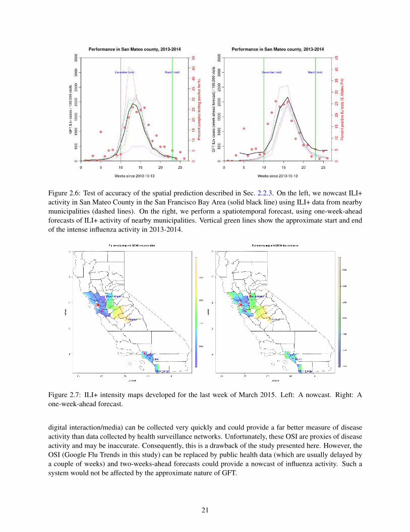
Figure 2.6: Test of accuracy of the spatial prediction described in Sec. 2.2.3. On the left, we nowcast ILI+activity in San Mateo County in the San Francisco Bay Area (solid black line) using ILI+ data from nearbymunicipalities (dashed lines). On the right, we perform a spatiotemporal forecast, using one-week-aheadforecasts of ILI+ activity of nearby municipalities. Vertical green lines show the approximate start and endof the intense influenza activity in 2013-2014.

Figure 2.7: ILI+ intensity maps developed for the last week of March 2015. Left: A nowcast. Right: Aone-week-ahead forecast.

digital interaction/media) can be collected very quickly and could provide a far better measure of diseaseactivity than data collected by health surveillance networks. Unfortunately, these OSI are proxies of diseaseactivity and may be inaccurate. Consequently, this is a drawback of the study presented here. However, theOSI (Google Flu Trends in this study) can be replaced by public health data (which are usually delayed bya couple of weeks) and two-weeks-ahead forecasts could provide a nowcast of influenza activity. Such asystem would not be affected by the approximate nature of GFT.

21

Figure 2.8: A snapshot of the output of the data assimilation system, displayed as a web page on an internalSandia server.

22

We also investigated whether the well-known dependence of influenza activity on meteorological vari-ables [20] could be used to spatially predict said activity from municipalities with data and produce influenzaactivity maps. It required a new spatial prediction scheme using climatologically averaged temperature andspecific humidity, as well as kernel smoothing. We tested this hypothesis in SFBA and our preliminaryresults have been encouraging when compared to public health data from San Mateo County. The methodwas extended to target 3 population centers in California (SFBA being one) and produce influenza activitymaps, but we do not have independent public health data to test the accuracy of the spatial prediction methodin the other two clusters.

The data assimilation system was implemented as a prototype and run weekly on a Sandia server for a year. Itproduced influenza activity maps for a year (2014-2015) and was stopped when GFT stopped publishing itsdata. It required little manual intervention and demonstrates that as long as OSI are available, such localizeddata assimilation systems can be constructed and deployed in the cloud. This could be very helpful incountries/areas with poor public health reporting. Collecting digital proxies of disease activity (web searchlogs, media articles pertaining to an outbreak etc.) is a well-established activity and global meteorologicalreanalysis products are easily available (e.g., Goddard Earth Sciences Data and Information Sciences Center,http://disc.sci.gsfc.nasa.gov/mdisc/data-holdings). Our method provides a way of combiningthese datastreams, along with disease models, to provide information of epidemiological and public healthrelevance.

23

24

Chapter 3

Data assimilation for dengue

3.1 Introduction

Dengue is a tropical disease spread by mosquitoes, typically Aedes aegypti [44]. In India, the dengue seasonfollows the rainy monsoon season in the middle of the year. The monsoons sweep in from the Arabian Sea,in a Southwest-to-Northeast direction, leading to rains after the Indian summer. Mosquitoes and denguesoon follow [45, 46, 47, 48].

There have been attempts to track dengue activity using open source indicators (OSI). Web search logshave been used to track dengue in southeast Asia [49], using a model that linearly related the frequencyof search to dengue incidence, as obtained from public health reports. The same study found that dataobtained at a weekly resolution was preferable. Google Dengue Trends (GDT) provided a service (whichlasted till August 2015) that tracked dengue in a number of countries [50]. Data was provided aggregatedat the national scale, though for certain countries e.g., Mexico, provincial data was also available. In [51],the authors used provincial GDT data from Mexico to (1) compare against public health data and (2) elicitthe effect of climate on dengue incidence. GDT data was found to be in good agreement with public healthdata, and a dependence on climatic factors was identified, with a lag of 8 weeks i.e., meteorological variableswere a leading indicator. In a follow-on publication [52], they showed that the agreement between GDT andpublic health data was better in regions with intense dengue activity; including climatic factors in the modelplayed a small part in improving predictive skill. In [53], the authors used alerts from HealthMap (https;//www.healthmap.org; HM), caused by an excessive number of media articles, open-source documentsetc. on dengue, to track dengue in Latin America. They used kernel smoothing to create proxies of dengueincidence maps, but did not exploit dengue’s dependence on climatic factors in the spatial prediction models.

Dengue’s dependence on the presence of its vector limits it to regions where the Aedes aegypti mosquitois present. The mosquito does not have much of a flight range and consequently dengue cases tend tocluster. A temporal variation is imposed by weather which controls the breeding of mosquitoes. Dengueincidence data (time and location of individual cases) have been subjected to clustering analysis in space-time [54, 55], using Knox-like tests to detect clusters [56]. The analysis is used to compute dengue riskto the population by convolving it with population density maps [57]. Incidence data collated over arealunits have been used to make risk maps via kernel smoothing [58, 59]. Socioeconomic, environmental andland-use patterns are also factors in dengue prediction, and serve as exogenous variables in dengue riskmapping. The continuous variables (socioeconomic and environmental factors) are generally included vialinear regression [60], while land-use categories are assimilated using logistic regression [61]. Conditionallyauto-regressive (CAR) models with Poisson noise (to model dengue incidence counts) have been used forthe spatial mapping of dengue risks [62], as have Gaussian processes in space-time [63]. However, there donot seem to be any studies that use statistical methods on provincial GDT or HM data to compute dengue

25

risk maps (using climatic factors as exogenous variables), to impute missing data or to forecast a risk/dengueincidence map.

In this study we investigate a method to create maps (nowcasts and forecasts) of dengue activity in India.The OSI of relevance is obtained from HM. HM scrapes the Web for documents - media articles, Ministry ofHealth publications, ProMed Mail articles - that concern dengue and makes the data available dis-aggregatedby date and state. Only articles in English are collected and thus we obtain a small sampling of the totaldengue-related media activity. Many of the media articles are duplicates, reprints from the same articleobtained from news agencies such as Reuters (https://www.reuters.com). These duplicates are retained.We also use re-analysis products, temperature and precipitation fields obtained from[64].

Our mapping method is based on the hypothesis, similar to the one behind GFT and GDT, that dengue-related media activity is correlated to people’s interest in the topic, which in turn could be caused by adengue outbreak. Further, dengue activity would be correlated with temperature and rainfall, perhaps witha time lag required by mosquitoes to breed and spread dengue. Collating the data on a state-by-state basiscould allow one to provide forecasts using time-series methods, with precipitation and temperature actingas exogenous factors/predictors.

3.2 Materials and methods

In this section we describe the data, its shortcomings and the modeling requirements for constructing dengueactivity maps.

3.2.1 Data

MERRA (Modern Era Retrospective-analysis for Research and Applications) meteorological reanalysis dataused in this study - temperature at 2m above ground and precipitation - are obtained from [64]. Thesereanalysis gridded datasets (0.5× 0.67 degree resolution) are available for every hour and are averaged totheir monthly values. Data from HM was purchased and provided us with dengue data for 2011 - 2013. Thedata was disaggregated by state and we computed monthly figures for the counts of media articles etc. Thedata was sparse and few states, over a month, exceeded 50 media mentions. Further, no data was availablebefore August 2011, providing us with 29 months of data, in all.

The HM data was gappy i.e., there were months in the dengue season where a state ostensibly recordedno media article on the topic. Further there was no pattern in the “missingness” of the data. Fig. 3.1 plotsthe number of HM articles for India for October 2011, 2012 and 2013. The north Indian states (left blank)recorded no media articles. For the rest, we binned the HM counts and shaded the states accordingly. Only15 states had any data at all, and we will focus our forecasting efforts on this subset. It is clear that the HMdata is missing at random (MAR). However, meteorological data is available everywhere and is correlatedwith HM data. Filling the missing HM data is a pre-requisite for performing time-series predictions on astate-by-state level for the subset of 15 Indian states. Of the 15×29 = 435 possible data points, about 60%were missing.

26

Figure 3.1: Plots of the binned counts of HM articles on dengue for India for October 2011 (left), 2012(middle) and 2013 (right). The blank states recorded no data. States with data are shaded with a colorcorresponding to the lower bound of their bin. We see missing data occurs at random.

3.2.2 Conditionally auto-regressive models

The HM dataset contained “holes” - missing data points which were surrounded in time by observed datapoints. We constructed a neighborhood matrix for each state - any state that shared a border was deemed aneighbor. This 15× 15 matrix W has an “1” entry if two states abut each other, else the matrix element iszero. This revealed that a missing data point often had observed data in a few of its neighbors. In order toimpute a value for a missing data point, it was necessary to impose a spatio-temporal model. We performedthis using conditionally auto-regressive models [29, 30, 31]. We provide a summary of the space-timeconditionally auto-regressive model (STCAR) below.

Let Ykt be the count for state k and time t. We model it as a draw from a normal distribution N (:, :)

Ykt |µµµkt ∼N (µµµkt ,ν2), where µµµkt = Xktβββ+φkt , βββ∼N (µβββ,Σβββ), k = 1 . . .K, and t = 1 . . .T. (3.1)

Here Xkt is a 1×2 vector containing temperature and precipitation for the state k and time t and βββ= {βT ,βP},the regression weights for the meteorological variables. φkt models the correlation in space-time and ν2 isthe observation error variance, modeled with an Inverse-Gamma (InvGamma(1.0, 0.01)) prior.

Let φφφt = {φkt}, k = 1 . . .K, K = 15. The model for φφφ is

φφφt |φφφt−1 ∼ N (ρ1φφφt−1,τ2Q(W,ρ2)

−1)

φφφ1 ∼ N (0,τ2Q(W,ρ2)−1)

τ2 ∼ InvGamma(1,0.01)

ρ1,ρ2 ∼ U(0,1) (3.2)

Thus temporal correlation is modeled by the mean ρ1φφφt−1 and spatial autocorrelation by the varianceτ2Q(W,ρ2). The precision matrix Q(W,ρ2) is given by

Q(W,ρ2) = ρ2 (diag(W1)−W)+(1−ρ2)I

where I is a 15×15 identity matrix.

This model is fitted i.e., βββ,ρ1,ρ2,τ2 are estimated from the available data using an Markov chain Monte

Carlo approach. The R [65] package CARBayesST [66] was used for the purpose.

27

3.2.3 Boosting

The STCAR model did not provide very accurate estimates and we resorted to boosting using Friedman’sgradient boosting [67]. Consider a response Y with a set of predictors X. Our aim to estimate a mappingY = f (X) by minimizing the expectation of a loss function Ψ(Y, f )

f (X) = argmin f (X) (Ey,xΨ(y, f ))

The procedure is as follows. We set f (x) to a constant. Then for t = 1 . . .T , do the following

1. Compute the negative gradient

zi =−∂

∂ f (X)Ψ(y, f (X))

∣∣∣f (Xi)

2. Fit a model g(X) that predicts zi from Xi

3. Choose a gradient descent step ∆

∆ = argmin∆

N

∑i=1

Ψ(Y, f (Xi)+∆g(Xi))

4. Update the estimate of f (X)

f (X) = f (X)+∆g(X)

5. Repeat the steps above till the successive difference between f (X) become smaller than a tolerance.

The boosted STCAR models provide a means of obtaining “filled-in” datasets for each of the states. There-after, we fit a seasonal auto-regressive integrated moving average model with exogenous inputs (SARIMAX;see Chapter 8 in [68]) to each state’s data and provide a forecast, along with a predictive error bound.

3.3 Results

Imputation accuracy was compared between a traditional, non-boosted STCAR approach and the boostedapproach, where the base learner was a STCAR model. The data from the last three months of 2013 wereheld-out and used for testing the boosted STCAR models. Tests were performed for each state separatelyand then averaged for an overall performance figure. The resultant RMSEs (root mean square errors) fromthe cross-validation procedure are given in Fig. 3.2. Overall, the boosted setting performs better than thenon-boosted setting by a factor of nearly two. We observe variability in the relative performance of thenon-boosted and boosted settings across states, but we were unable to identify the phenomenon responsiblefor this variability. It does not appear that these differences in relative performance are related to the amountof missingness or the extremity of the values we were trying to predict.

A comparison between the observed data set with missing values and the resultant fully-imputed data setusing boosting are shown in Fig. 3.3. The seasonal trends are expected given the seasonal nature of dengue

28

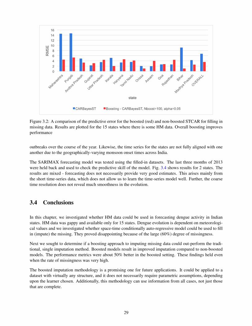
Figure 3.2: A comparison of the predictive error for the boosted (red) and non-boosted STCAR for filling inmissing data. Results are plotted for the 15 states where there is some HM data. Overall boosting improvesperformance

outbreaks over the course of the year. Likewise, the time series for the states are not fully aligned with oneanother due to the geographically-varying monsoon onset times across India.

The SARIMAX forecasting model was tested using the filled-in datasets. The last three months of 2013were held back and used to check the predictive skill of the model. Fig. 3.4 shows results for 2 states. Theresults are mixed - forecasting does not necessarily provide very good estimates. This arises mainly fromthe short time-series data, which does not allow us to learn the time-series model well. Further, the coarsetime resolution does not reveal much smoothness in the evolution.

3.4 Conclusions

In this chapter, we investigated whether HM data could be used in forecasting dengue activity in Indianstates. HM data was gappy and available only for 15 states. Dengue evolution is dependent on meteorologi-cal values and we investigated whether space-time conditionally auto-regressive model could be used to fillin (impute) the missing. They proved disappointing because of the large (60%) degree of missingness.

Next we sought to determine if a boosting approach to imputing missing data could out-perform the tradi-tional, single imputation method. Boosted models result in improved imputation compared to non-boostedmodels. The performance metrics were about 50% better in the boosted setting. These findings held evenwhen the rate of missingness was very high.

The boosted imputation methodology is a promising one for future applications. It could be applied to adataset with virtually any structure, and it does not necessarily require parametric assumptions, dependingupon the learner chosen. Additionally, this methodology can use information from all cases, not just thosethat are complete.

29

Figure 3.3: Top: The raw HealthMap data with gaps in it. Bottom: Filled in version of the HealthMapdataset.

30

Forecasts from ARIMA(0,0,0) with zero mean

Date

HM

2011.5 2012.0 2012.5 2013.0 2013.5

−20

24

68

10

●●

Forecasts from ARIMA(1,0,0) with zero mean

Date

HM

2011.5 2012.0 2012.5 2013.0 2013.5

05

1015

2025

30

●

●

Figure 3.4: Left: Forecast of the HM data, for the state of Kerala. The blue dot is the mean prediction, withthe shaded error being the 90% and 99% credibility intervals. The red dot is the true (not filled in) value.Right: The same, but for the state of Maharashtra.

One limitation of the boosting imputation methodology is that the time required to obtain boosted impu-tations is linearly related to the number of boosting iterations specified. If a base learner model takes asubstantial amount of time to fit, then boosting it could potentially be memory and time consuming. Morework is required to ascertain the robustness of these methods under various data conditions such as missing-ness mechanism, data structure, distribution, and missingness in multiple variables. Future efforts shouldfocus on assessment of the robustness of the method and potential improvements that might be made byusing adaptive boosting algorithms

The imputed datasets were then used in SARIMAX modeling. Results were not encouraging primarilybecause the datasets were too short to learn a good SARIMAX model. If the HM articles were morecopious, allowing us to aggregate on a weekly rather than monthly basis, and if the dataset spanned a largerduration, we believe forecasting results would have displayed smaller predictive errors.

31

32

Chapter 4

Follow-on applications

In this chapter, we discuss some work that incorporated or built on the methods or approaches developed inour study.

4.1 Data assimilation for wildfires

The data assimilation architecture described in Chp. 2 is sufficiently general that the models and data streamscan be replaced so that the same general philosophy can be used in a very different setting. One such settingis crisis management where sparse data is usually available but not with sufficient accuracy or completenessto allow good situational awareness. Models of many types of crises and their consequences to society doexist (mostly for planning a response). It raises the question whether data, along with a model, could “fillin” the missing information. This could lead to a situational awareness toolkit containing both nowcastingand forecasting capabilities.

SUMMIT (Standard Unified Modeling and Mapping Integration Toolkit, [69]) is a Sandia framework forintegrating models used in crisis management. It is also designed to wrap third-party models and allowcommunication and interactions between them, mainly to allow response planning. It also has the capabilityto to collect live datastreams and contains numerous visualization tools to display the results of modelexecutions. To date, it has not had the capability to exploit data streams, perhaps with models, to inferinformation about the crisis that is not readily apparent from the raw data.

To that end, we are incorporating a data assimilation capability (algorithmically similar to Chp. 2) to fill inunobserved data (the aim for Chp. 3). As a first step, we enabled SUMMIT to provide access to the resultsof the temporal data assimilation capability described in Chp. 2 (ETKF and SIR model of influenza). Thisrequired extension of SUMMIT to accommodate the peculiar interaction between models and data that are ahallmark of ETKF and visualization of probabilistic forecasts. It also allowed us to set out design enhance-ments SUMMIT would require to evolve into a crisis management tool where uncertainty in situationalawareness (and the consequent impact on response planning) are fully and rigorously accommodated.

The next step was a more difficult exercise where we performed data assimilation and probabilistic forecast-ing for wildfires using a model that SUMMIT hosts. FARSITE [70] is a wildfire modeling tool developedby the US Department of Agriculture. It uses meteorological inputs (wind, humidity etc.) and vegetation(fuel) parameters to provide time-resolved evolution of a fire front, modeled as a set of perimeter points. Themodel adaptively refines the fire front as it expands so that the spatial resolution does not suffer. FARSITEis generally used to compute one-day-ahead forecasts of the fire front, using an infra-red image of the fire(obtained using overflights by spotter airplanes) as the initial condition. The initial condition is assumeddeterministic i.e., neither ensemble simulations nor data assimilation are currently performed to obtain fore-

33

Figure 4.1: The wildfire after two hours. No observational data have been assimilated. The spread in forecastfire fronts (red contours) are due to our ignorance of wind and initial conditions. The blue contour is thetrue fire front.

casts. We enabled data assimilation with FARSITE by encoding a particle filter [71] to drive FARSITE.The data assimilation system ingests sparse observational data on the location of the fire front (i.e, data onwhere the fire has been observed) and meteorological data (wind and humidity available at a few locations)to provide updated (i.e., data informed) estimates of the full fire front and wind information. The ensembleof approximately 100 FARSITE instances (that reflects our ignorance of initial conditions, meteorology andfuel/vegetation parameters) is continuously updated to agree with sparse observational data and then used toprovide forecasts.

We tested the data assimilation system using synthetic data from a fire near Santa Monica, California.Fig. 4.1 shows the fire front after two hours; both the true perimeter and the spread of 100 ensemble sim-ulations are shown overlaid on a satellite image. Fig. 4.2 shows the true and forecasted fire front afterfive hours. The importance of probabilistic forecasting is seen in Fig. 4.3 where the uncertainty spread inforecasts includes residences.

SUMMIT’s development (which included the ability to wrap and orchestrate the interaction between mod-els, access and incorporate data streams as well as visualization) was funded over a period of time (approxi-mately five years) by US Department of Homeland Security, S&T Division. The data assimilation capabilityis novel, but still prototypical. It has not been tested with real data, which will inevitably require new modelsfor observational errors. The sensitivity of the data assimilation system to sparseness of observational dataas well as the impact of outlier observations is not known. Further, it is unknown how large an ensemble

34

Figure 4.2: The wildfire after five hours. Data assimilation has occurred and reduces the uncertainty spread.The snapshot shows results displayed in SUMMIT’s web client. The red contours are the 5 hour forecastswithout data assimilation. A very narrow ensemble of purple fire fronts, very near the blue (true) fire front(and difficult to see) is the forecast ensemble, after assimilating data available after two hours.

should be to deliver a given forecasting accuracy, as well as to be numerically stable. In order to developthese capabilities, we will explore funding opportunities with California Department of Forestry and FireProtection (https://www.fire.ca.gov) in 2017.

4.2 Data assimilation and disease modeling

The description in Chapters 2 and 3 provide a glimpse of the various approaches being pursued to exploitopen-source indicators to track and forecast outbreaks. However, it has been noted that such models oftenproduce conflicting forecasts. Further, an ensemble of such models can provide even more confusion sincethe disagreement between model predictions are not uniform i.e., subsets of models might agree. However,it is unclear whether the agreement is due to a similarity/correlation between the data streams being as-similated and the structure of the models (in which case, the agreement between models produces no newinformation) or if the agreement reflects some underlying truth. Sandia has been funded to address thisproblem. Our ability to calibrate disease models to open-source data-stream (as described in Chp. 2 and 3)and thus construct an ensemble is a prerequisite for performing this work, and the ease with which we couldconstruct the ensemble played a role in the success of our proposal to the Defense Threat Reduction Agency.The work starts in FY17.

35

Figure 4.3: The wildfire after five hours, in detail. The uncertainty spreads show risk to human habita-tion and reinforce the need for data assimilation and probabilistic forecasting using filtering methods. Thepurple ensemble is easy to see and shows the enormous decrease in forecasting uncertainty effected by theassimilation of data after two hours.

36

Chapter 5

Conclusions

In this study we have investigated the use of open-source indicators to track and forecast epidemiologicalactivity. In particular, we have explored the types of data assimilation systems that might be required to inferuseful information about epidemiological dynamics. Our first foray, described in Chp. 2, may be consideredone end of the spectrum. Here completeness of the observational data is not an issue. Rather, one questionswhether the choice of data stream i.e., web search logs serving as proxies of disease activity is justified, andhow disease models may be pressed into inferring disease dynamics and forecasting. The emphasis lies onsophisticated data science methods, disease models and forecasting accuracy.

Data assimilation for dengue, as described in Chp. 3, forms the other end of the spectrum where the ob-servational data is spotty and emphasis lies in filling in the missing data. We have developed a techniquethat uses two open-source indicators - data from HealthMap and meteorology, to complete observationaldatasets. The actual forecasting is performed using simple time-series methods. Both the data assimilationmethods (Chp. 2 and 3) produce disease activity maps, but the two systems have nothing in common intheir need for methodological sophistication. This is because the data assimilation systems, practically, aredesigned to compensate for the shortcomings of the data streams when inferring disease activity maps. Theywill therefore be disease and location-specific. However, structurally, they will all contain disease models,calibration methodologies and missing-data imputation technologies, but their particular implementations(and algorithmic choices) will vary depending on the datastreams at hand.

The techniques developed in this study find many uses. The ETKF and thereafter particle filters have beenimplemented in a software framework for crisis management. The ability to construct calibrated diseasemodels that ingest open-source information has led to a funded project to assess the worth of disease modelsthat “work off” different data streams (Chp. 4). Thus while the question of data assimilation for diseaseforecasting is indeed an interesting one, the importance (and worth) of the project lies in the developmentof methodological sophistication in Sandia’s data science’s capabilities. It is a fundamental strength and, asshown in Chp. 4, is being leveraged in myriad unexpected ways.

37

This page intentionally left blank

38

References

[1] World Health Organization Inflenza (Seasonal) factsheet. http://www.who.int/mediacentre/factsheets/fs211/en/.

[2] CDC Flu View. https://www.cdc.gov/flu/weekly/.

[3] J. Ginsberg, M. H. Mohebbi, R. S. Patel, L. Brammer, and M. S. Smolinski. Detecting influenzaepidemics using search engine query data. Nature, 457:1012–1014, 2009.

[4] Influenza National and Regional Level Graphs and Data. http://gis.cdc.gov/grasp/fluview/fluportaldashboard.html.

[5] P. M. Pohlgreen, Y. Chen, D. M. Pennock, F. D. Nelson, and R. A. Weinstein. Using Internet searchesfor influenza surveillance. Clinical Infectious Diseases, 47(11):1443–1448, 2008.

[6] M. J. Paul, M. Dredze, and D. Broniatowski. Twitter improves influenza forecasting. PLOS CurrentsOutbreaks, (1), 2014.

[7] V. Lampos and N. Cristianini. Nowcasting events from the Social Web with statistical learning. ACMTransactions on Intelligent Systems and Technology, 3(4), 2012. Article 72.

[8] D. J.McIver and J. S. Brownstein. Wikipedia usage estimates prevalence of influenza-like illness in theunited states in near real-time. PLoS Comput Biology, 10(4):1–8, 04 2014.

[9] N. Generous, G. Fairchild, A. Deshpande, S. Y. Del Valle, and R. Priedhorsky. Global disease moni-toring and forecasting with wikipedia. PLoS Comput Biology, 10(11):1–16, 11 2014.

[10] M. Santillana, E. O. Nsoesie, S. R. Mekaru, D. Scales, and J. S. Brownstein. Using clinicians searchquery data to monitor influenza epidemics. Clinical Infectious Diseases, 59(10):1446–1450, 2014.

[11] D. R. Olson, K. J. Konty, M. paladini, C. Viboud, and L. Simonsen. Reassessing Google Flu Trendsdata for detection of seasonal and pandemic influenza: A comparative epidemiological study at threegeographic scales. Public Library of Science, Computational Biology, 9(10), 2013. e1003256.

[12] D. Lazer, R. Kennedy, G. King, and A. Vespignani. The parable of Google Flu: Traps in big dataanalysis. Science, 343(6176):1203–1205, 2014.

[13] Patrick Copeland, Raquel Romano, Tom Zhang, Greg Hecht, Dan Zigmond, and Christian Stefansen.Google disease trends: An update. In International Society of Neglected Tropical Diseases 2013,page 3, 2013.

[14] S. Cook, C. Conrad, A. Fowlkes, and Matthew H. M. H. Mohebbi. Assessing Google Flu Trendsperformance in the united states during the 2009 influenza virus A (H1N1) pandemic. PLoS ONE,6(8):1–8, 08 2011.

[15] S. Yang, M. Santillana, and S. C. Kou. Accurate estimation of influenza epidemics using Google searchdata via ARGO. Proceedings of the National Academy of Sciences, 112(47):14473–14478, 2015.

39

[16] Mauricio Santillana, D. Wendong Zhang, Benjamin M. Althouse, and John W. Ayers. What can dig-ital disease detection learn from (an external revision to) Google Flu Trends? American Journal ofPreventive Medicine, 47(3):341 – 347, 2014.

[17] M. Santillana, A. T. Nguyen, M. Dredze, M. J. Paul, E. O. Nsoesie, and J. S. Brownstein. Combiningsearch, social media, and traditional data sources to improve influenza surveillance. PLoS ComputBiology, 11(10):1–15, 10 2015.

[18] P. Chakraborty, P. Khadivi, B. Lewis, A. Mahendiran, J. Chen, P. Butler, E. O. Nsoesie, S. R. Mekaru,J. S. Brownstein, M. V. Marathe, and N. Ramakrishnan. Forecasting a Moving Target: EnsembleModels for ILI Case Count Predictions, chapter 30, pages 262–270. 2014.

[19] Z. Wang, P. Chakraborty, S. R. Mekaru, , J. S. Brownsteinand J. Ye, and N. Ramakrishnan. Dynamicpoisson autoregression for influenza-like-illness case count prediction. In Proceedings of the 21thACM SIGKDD International Conference on Knowledge Discovery and Data Mining, KDD ’15, pages1285–1294, New York, NY, USA, 2015. ACM.

[20] J. D. Tamerius, J. Shaman, W. J. Alonso, K. Bloom-Feshbach, C. K. Uejio, A. Comrie, and C. Viboud.Environmental predictors of seasonal influenza epidemics across temperate and tropical climates. PLoSPathog, 9(3):1–12, 03 2013.

[21] R. P. Soebiyanto, F. Adimi, and R. K. Kiang. Modeling and predicting seasonal influenza transmissionin warm regions using climatological parameters. Public Library of Science, One, 5:e9450, 2010.

[22] Jeffrey Shaman and Alicia Karspeck. Forecasting seasonal outbreaks of influenza. Proceedings of theNational Academy of Science of the United States, 109(50), 2012. doi:10.1073/pnas.1208772109.

[23] J. Shaman, A. Karspeck, W. Yang, J. Tamerius, and M. Lipsitch. Real-time influenza forecasts duringthe 2012-2013 season. Nature Communications, 4, 2013. 2837.

[24] E. Goldstein, C. Viboud, V. Charu, and M. Lipsitch. Improving the estimation of influenza-relatedmortality over a seasonal baseline. Epidemiology, 23(6):829838, 2012.

[25] W. Yang, A. Karspeck, and J. Shaman. Comparison of filtering methods for the modeling and retro-spective forecasting of influenza epidemics. PLoS Comput Biology, 10(4):1–15, 04 2014.

[26] L. Waller and B. Carlin. Disease mapping. In A. E. Gelfand, P. J. Diggle, M. Fuentes, and P. Guttorp,editors, Handbook of Spatial Statistics. Chapman & Hall / CRC Press, 2010.

[27] J. Besag, J. C. York, and A. Mollie. Bayesian image restoration, with two applications in spatialstatistics (with discussion). Annals of the Institute of Statistical Mathematics, 43, 1991.

[28] L. Held, M. Hohle, and M. Hofmann. A statistical framework for the analysis of multivariate infectiousdisease surveillance counts. Statistical Modelling, 5(3):187–199, 2005.

[29] Duncan Lee. A comparison of conditional autoregressive models used in Bayesian disease mapping.Spatial and Spatio-temporal Epidemiology, 2(2):79 – 89, 2011.

[30] D. Lee, A. Rushworth, and S. K. Sahu. A Bayesian localized conditional autoregressive model forestimating the health effects of air pollution. Biometrics, 70(2):419–429, 2014.

[31] A. Rushworth, D. Lee, and R. Mitchell. A spatio-temporal model for estimating the long-term effectsof air pollution on respiratory hospital admissions in Greater London. Spatial and Spatio-temporalEpidemiology, 10:29 – 38, 2014.

40

[32] Ransalu Senanayake, Simon OCallaghan, and Fabio Ramos. Predicting spatio–temporal propagationof seasonal influenza using variational Gaussian Process regression. In Thirtieth AAAI Conference onArtificial Intelligence, 2016.

[33] M. B. Hooten, J. Anderson, and L. A. Waller. Assessing North American influenza dynamics with astatistical SIRS model. Spatial and Spatio-temporal Epidemiology, 1(23):177 – 185, 2010. GEOMEDConference.

[34] M. W. Davidson, D. A. Haim, and J. M. Radin. Using networks to combine big data and traditionalsurveillance to improve influenza predictions. Scientific Reports, 2015. Published 2015/01/29/online.

[35] Y. Xia and et al. NCEP/EMC, NLDAS Primary Forcing DataL4 Hourly 0.125 x 0.125 degree V002, version 002, 2009.http://disc.sci.gsfc.nasa.gov/uui/datasets/NLDAS FORA0125 H V002/summary?keywords=NLDAS#prod-summary.

[36] B. A. Cosgrove, D. Lohmann, K. E. Mitchell, P. R. Houser, E. F. Wood, J. C. Schaake, A. Robock,C. Marshall, J. Sheffield, Q. Duan, L. Luo, R. W. Higgins, R. T. Pinker, J. D. Tarpley, and J. Meng.Real-time and retrospective forcing in the North American Land Data Assimilation System (NLDAS)project. Journal of Geophysical Research: Atmospheres, 108(D22), 2003. 8842.

[37] Google Flu Trends. https://www.google.org/flutrends/about.

[38] National and regional level outpatients illness and viral surveillance.http://gis.cdc.gov/grasp/fluview/fluportaldashboard.html.

[39] C. H. Bishop, B. J. Etherton, and S. J. Majumdar. Adaptive sampling with the ensemble transformKalman filter. Part i: Theoretical aspects. Monthly Weather Review, 129(3):420–436, 2001.

[40] Pavel Sakov. EnKF-Matlab: Matlab code for ensemble Kalman filter, with a number of simple models,version 0.31. https://enkf.nersc.no.

[41] J. Shaman and M. Kohn. Absolute humidity modulates influenza survival, transmission and seasonal-ity. Proceedings of the National Academy of Science, USA, 106:3243–3248, 2009.

[42] J. Shaman, V. E. Pitzer, C. Viboud, B. T. Grenfell, and M. Lipsitch. Absolute humidity and the seasonalonset of influenza in the continental United States. Public Library of Science Biology, 8:e1000316,2010.

[43] T. Hastie, R. Tibshirani, and J. Friedman. The Elements of Statistical Learning. Springer Series inStatistics. Springer New York Inc., New York, NY, USA, 2008.

[44] Dengue fever, Wikipedia, the free encyclopedia. https://en.wikipedia.org/wiki/Dengue fever.

[45] P. Aggarwal, P. Gupta, S. D. Kandpal, B. Kakati, and D. Gupta. Post-monsoon season surveillance amust for curtaling annual dengue epidemic in rural India. Journal of Community Medicine, 5(1):153–155, 2014.

[46] S. Chandy, K. Ramanathan, A. Manoharan, D. Mathai, and K. Baruah. Assessing effect of climateon the incidence of dengue in Tamil Nadu. Indian Journal of Medical Microbiology, 13(3):283–286,2013.

[47] K. Durani, J. Dund, H. Shingala, and M. Sinha. Epidemiological trend analysis of dengue virus infec-tion in western part of Gujarat. Indian Journal of Research, 3(6):146–148, 2014.

41

[48] S. Jeelani and S. Sabesan. Aedes vector population dynamics and occurence of dengue fever in relationto climate variables in Puducherry, South India. International Journal of Current Microbiology andApplied Sciences, 2(12):313–322, 2013.

[49] Emily H Chan, Vikram Sahai, Corrie Conrad, and John S Brownstein. Using web search query data tomonitor dengue epidemics: a new model for neglected tropical disease surveillance. PLoS Negl TropDis, 5(5):e1206, 2011.

[50] Google Flu Trends. https://www.google.org/flutrends/about.

[51] Rebecca T Gluskin, Mauricio Santillana, and John S Brownstein. Using Google Dengue Trends toestimate climate effects in Mexico. Online journal of public health informatics, 5(1), 2012.

[52] Rebecca Tave Gluskin, Michael A Johansson, Mauricio Santillana, and John S Brownstein. Evaluationof internet-based dengue query data: Google Dengue Trends. PLoS Negl Trop Dis, 8(2):e2713, 2014.

[53] Anne G Hoen, Mikaela Keller, Aman D Verma, David L Buckeridge, and John S Brownstein. Elec-tronic event-based surveillance for monitoring dengue, latin america. Emerg Infect Dis, 18(7):1147–50,2012.

[54] S. Thammapalo, V. Chongsuvivatwong, A. Geater, and M. Dueravee. Environmental factors and inci-dence of dengue fever and dengue haemorrhagic fever in an urban area, southern thailand. Epidemiol-ogy and Infection, 136(1):135–143, 03 2007.

[55] Camilo Rotela, Florence Fouque, Mario Lamfri, Phillipe Sabatier, Virginia Introini, Mario Zaidenberg,and Carlos Scavuzzo. Spacetime analysis of the dengue spreading dynamics in the 2004 Tartagaloutbreak, Northern Argentina. Acta Tropica, 103(1):1 – 13, 2007.

[56] Martin Kulldorff and Ulf Hjalmars. The Knox method and other tests for space-time interaction.Biometrics, 55(2):544–552, 1999.

[57] Mohammad Ali, Yukiko Wagatsuma, Michael Emch, and Robert F Breiman. Use of a geographicinformation system for defining spatial risk for dengue transmission in Bangladesh: role for Aedesalbopictus in an urban outbreak. The American journal of tropical medicine and hygiene, 69(6):634–640, 2003.

[58] Florisneide R Barreto, Maria Gloria Teixeira, N Costa Maria da Conceicao, Marilia S Carvalho, andMauricio L Barreto. Spread pattern of the first dengue epidemic in the city of Salvador, Brazil. BMCPublic Health, 8(1):1, 2008.

[59] Joao B Siqueira, Celina MT Martelli, Ivan J Maciel, Renato M Oliveira, Maria G Ribeiro, Fluvia PAmorim, Bruno C Moreira, Divina DP Cardoso, Wayner V Souza, and Ana Lucia SS Andrade. House-hold survey of dengue infection in central Brazil: spatial point pattern analysis and risk factors assess-ment. The American journal of tropical medicine and hygiene, 71(5):646–651, 2004.

[60] Adriano Mondini, Francisco Chiaravalloti Neto, Gallo Y Sanches, Jose Carlos Cacau Lopes, et al.Spatial analysis of dengue transmission in a medium-sized city in Brazil. Revista de Saude Publica,39(3):444–451, 2005.

[61] Birgit HB Van Benthem, Sophie O Vanwambeke, Nardlada Khantikul, Chantal Burghoorn-Maas,Kamolwan Panart, Linda Oskam, Eric F Lambin, and Pradya Somboon. Spatial patterns of and riskfactors for seropositivity for dengue infection. The American journal of tropical medicine and hygiene,72(2):201–208, 2005.

42

[62] Gustavo S Ferreira and Alexandra M Schmidt. Spatial modelling of the relative risk of dengue fever inRio de Janeiro for the epidemic period between 2001 and 2002. Brazilian journal of Probability andStatistics, pages 29–47, 2006.

[63] Hwa-Lung Yu, Shang-Jen Yang, Hsin-Ju Yen, and George Christakos. A spatio-temporal climate-based model of early dengue fever warning in southern Taiwan. Stochastic Environmental Researchand Risk Assessment, 25(4):485–494, 2011.

[64] Goddard Earth Sciences Data and Information Sciences Center. Modern era retrospective-analysis forresearch and applications (merra). http://disc.sci.gsfc.nasa.gov/mdisc/data-holdings.

[65] R Core Team. R: A Language and Environment for Statistical Computing. R Foundation for StatisticalComputing, Vienna, Austria, 2016.

[66] Duncan Lee, Alastair Rushworth, and Gary Napier. CARBayesST: Spatio-Temporal Generalised Lin-ear Mixed Models for Areal Unit Data, 2016. https://CRAN.R-project.org/package=CARBayesST.

[67] J. H. Friedman. Stochastic gradient boosting. Computational Statistics and Data Analysis, 38(4):367–378, 2002.

[68] R. Hyndman and G. Athanasopoulos. Forecasting: principles and practice. OTexts, 2013. https://www.otexts.org/book/fpp.

[69] Lynn I. Yang. SUMMIT: Standard Unified Modeling and Mapping Integration Toolkit. SAND2016-4881C.

[70] FARSITE: Fire, Fuel and Smoke Science Program. https://www.firelab.org/project/farsite.

[71] K. Law, A. Stuart, and K. Zygalakis. Data Assimilation: A mathematical introduction. Springer, 2015.Texts in Applied Mathematics.

43

DISTRIBUTION:

1 Jaideep Ray, 08959 MS 91591 Katherine Cauthen, 06132 MS 11371 P. Finley, 06131 MS 11881 H. Smith, 06826 MS 13631 S. Lefantzi, 08959 MS 91521 Technical Library, 08944 (electronic) MS 0899

44

v1.38