Online Control of Active Camera Networks for Computer ...25 Online Control of Active Camera Networks...
40
25 Online Control of Active Camera Networks for Computer Vision Tasks ADRIAN ILIE, University of North Carolina at Chapel Hill GREG WELCH, University of North Carolina at Chapel Hill and University of Central Florida Large networks of cameras have been increasingly employed to capture dynamic events for tasks such as surveillance and training. When using active cameras to capture events distributed throughout a large area, human control becomes impractical and unreliable. This has led to the development of automated approaches for online camera control. We introduce a new automated camera control approach that consists of a stochastic performance metric and a constrained optimization method. The metric quantifies the uncertainty in the state of multiple points on each target. It uses state-space methods with stochastic models of target dynamics and camera measurements. It can account for occlusions, accommodate requirements specific to the algorithms used to process the images, and incorporate other factors that can affect their results. The optimization explores the space of camera configurations over time under constraints associated with the cameras, the predicted target trajectories, and the image processing algorithms. The approach can be applied to conventional surveillance tasks (e.g., tracking or face recognition), as well as tasks employing more complex computer vision methods (e.g., markerless motion capture or 3D reconstruction). Categories and Subject Descriptors: I.2.8 [Artificial Intelligence]: Problem Solving, Control Methods, and Search; I.4.9 [Image Processing and Computer Vision]: Applications; J.7 [Computers in Other Systems]: Command and Control General Terms: Algorithms, Experimentation, Measurement, Performance Additional Key Words and Phrases: Camera control, active camera networks, computer vision, surveillance, motion capture, 3D reconstruction ACM Reference Format: Adrian Ilie and Greg Welch. 2014. Online control of active camera networks for computer vision tasks. ACM Trans. Sensor Netw. 10, 2, Article 25 (January 2014), 40 pages. DOI: http://dx.doi.org/10.1145/2530283 1. INTRODUCTION Many computer vision applications, such as motion capture and 3D reconstruction of shape and appearance, are currently limited to relatively small environments that can be covered using fixed cameras with overlapping fields of view. There is demand to extend these and other approaches to large environments, where events can happen in multiple dynamic locations, simultaneously. In practice, many such large environments are sporadic: events only take place in a few regions of interest (ROIs), separated by re- gions of space where nothing of interest happens. If the locations of the ROIs are static, This work was supported by ONR grant N00014-08-C-0349 for Behavior Analysis and Synthesis for Intel- ligent Training (BASE-IT), led by Greg Welch (PI) at UNC, Amela Sadagic (PI) at the Naval Post-graduate School, and Rakesh Kumar (PI) and Hui Cheng (Co-PI) at Sarnoff. Roy Stripling, Ph.D., Program Manager. Authors’ addresses: A. Ilie, University of North Carolina at Chapel Hill, Department of Computer Science; email: [email protected]. G. Welch, University of North Carolina at Chapel Hill, Department of Computer Science; University of Central Florida Institute for Simulation & Training and Department of Electrical Engineering & Computer Science. Permission to make digital or hard copies of part or all of this work for personal or classroom use is granted without fee provided that copies are not made or distributed for profit or commercial advantage and that copies show this notice on the first page or initial screen of a display along with the full citation. Copyrights for components of this work owned by others than ACM must be honored. Abstracting with credit is permitted. To copy otherwise, to republish, to post on servers, to redistribute to lists, or to use any component of this work in other works requires prior specific permission and/or a fee. Permissions may be requested from Publications Dept., ACM, Inc., 2 Penn Plaza, Suite 701, New York, NY 10121-0701 USA, fax +1 (212) 869-0481, or [email protected]. c 2014 ACM 1550-4859/2014/01-ART25 $15.00 DOI: http://dx.doi.org/10.1145/2530283 ACM Transactions on Sensor Networks, Vol. 10, No. 2, Article 25, Publication date: January 2014.
Transcript of Online Control of Active Camera Networks for Computer ...25 Online Control of Active Camera Networks...
25
Online Control of Active Camera Networks for Computer Vision Tasks
ADRIAN ILIE, University of North Carolina at Chapel HillGREG WELCH, University of North Carolina at Chapel Hill and University of Central Florida
Large networks of cameras have been increasingly employed to capture dynamic events for tasks such assurveillance and training. When using active cameras to capture events distributed throughout a largearea, human control becomes impractical and unreliable. This has led to the development of automatedapproaches for online camera control. We introduce a new automated camera control approach that consists ofa stochastic performance metric and a constrained optimization method. The metric quantifies the uncertaintyin the state of multiple points on each target. It uses state-space methods with stochastic models of targetdynamics and camera measurements. It can account for occlusions, accommodate requirements specificto the algorithms used to process the images, and incorporate other factors that can affect their results.The optimization explores the space of camera configurations over time under constraints associated withthe cameras, the predicted target trajectories, and the image processing algorithms. The approach can beapplied to conventional surveillance tasks (e.g., tracking or face recognition), as well as tasks employingmore complex computer vision methods (e.g., markerless motion capture or 3D reconstruction).
Categories and Subject Descriptors: I.2.8 [Artificial Intelligence]: Problem Solving, Control Methods,and Search; I.4.9 [Image Processing and Computer Vision]: Applications; J.7 [Computers in OtherSystems]: Command and Control
General Terms: Algorithms, Experimentation, Measurement, Performance
Additional Key Words and Phrases: Camera control, active camera networks, computer vision, surveillance,motion capture, 3D reconstruction
ACM Reference Format:Adrian Ilie and Greg Welch. 2014. Online control of active camera networks for computer vision tasks. ACMTrans. Sensor Netw. 10, 2, Article 25 (January 2014), 40 pages.DOI: http://dx.doi.org/10.1145/2530283
1. INTRODUCTION
Many computer vision applications, such as motion capture and 3D reconstruction ofshape and appearance, are currently limited to relatively small environments that canbe covered using fixed cameras with overlapping fields of view. There is demand toextend these and other approaches to large environments, where events can happen inmultiple dynamic locations, simultaneously. In practice, many such large environmentsare sporadic: events only take place in a few regions of interest (ROIs), separated by re-gions of space where nothing of interest happens. If the locations of the ROIs are static,
This work was supported by ONR grant N00014-08-C-0349 for Behavior Analysis and Synthesis for Intel-ligent Training (BASE-IT), led by Greg Welch (PI) at UNC, Amela Sadagic (PI) at the Naval Post-graduateSchool, and Rakesh Kumar (PI) and Hui Cheng (Co-PI) at Sarnoff. Roy Stripling, Ph.D., Program Manager.Authors’ addresses: A. Ilie, University of North Carolina at Chapel Hill, Department of Computer Science;email: [email protected]. G. Welch, University of North Carolina at Chapel Hill, Department of ComputerScience; University of Central Florida Institute for Simulation & Training and Department of ElectricalEngineering & Computer Science.Permission to make digital or hard copies of part or all of this work for personal or classroom use is grantedwithout fee provided that copies are not made or distributed for profit or commercial advantage and thatcopies show this notice on the first page or initial screen of a display along with the full citation. Copyrights forcomponents of this work owned by others than ACM must be honored. Abstracting with credit is permitted.To copy otherwise, to republish, to post on servers, to redistribute to lists, or to use any component of thiswork in other works requires prior specific permission and/or a fee. Permissions may be requested fromPublications Dept., ACM, Inc., 2 Penn Plaza, Suite 701, New York, NY 10121-0701 USA, fax +1 (212)869-0481, or [email protected]© 2014 ACM 1550-4859/2014/01-ART25 $15.00
DOI: http://dx.doi.org/10.1145/2530283
ACM Transactions on Sensor Networks, Vol. 10, No. 2, Article 25, Publication date: January 2014.
25:2 A. Ilie and G. Welch
acceptable results can be obtained by straightforward replication of static camera se-tups used for small environments. However, if the locations of the ROIs are dynamic,coverage needs to be ensured throughout the entire volume. Using an increasing num-ber of fixed cameras is impractical due to concerns over increased requirements interms of computation and monetary cost, bandwidth and storage.
One practical solution to this problem is using active cameras to cover sporadicenvironments. Active cameras have been used in surveillance [Collins et al. 2000] andin computer vision fields such as motion capture [Davis 2002] and robotics [Davisonand Murray 2002]. What makes them versatile is their capability to change their panand tilt settings to aim in the direction of dynamic ROIs, and zoom in or out to bestenclose the ROIs in their field of view. However, this versatility comes at a price: in orderto capture dynamic events, active cameras need to be controlled online, in real time.Control decisions need to be made as events are happening, and to take into accountfactors such as target dynamics and camera capabilities, as well as requirements fromthe computer vision algorithms the images are captured for, such as preferred cameraconfigurations, capture durations and image resolutions.
We present an approach that controls a network of active cameras online, in realtime, such that they capture multiple events taking place simultaneously in a sporadicenvironment and produce the best possible images for processing using computer visionalgorithms. We approach camera control as an optimization problem over the space ofpossible camera configurations (combinations of camera settings) and over time, underconstraints derived from knowledge about the cameras, the predicted ROI trajectoriesand the computer vision algorithms the captured images are intended for. Optimizationmethods rely on objective functions that quantify the “goodness” of a candidate solution.For camera control, this objective function is a performance metric that evaluatesdynamic, evolving camera configurations over time.
The rest of the article is organized as follows. In Section 2 we present a few perfor-mance metrics and touch on their suitability for use with our method. We also list someprevious camera control methods encountered in surveillance applications. Section 3details our performance metric, and Section 4 describes our control method.Section 5 briefly describes how we incorporate task requirements into our approach. InSection 6 we present experimental results. We discuss some future work and concludethe article in Section 7.
Note: This article is an extended version of the results presented at ICDSC 2011 [Ilieand Welch 2011], and builds on research conducted for a doctoral thesis [Ilie 2010]. Itpresents the progress made in the meantime, with an emphasis on the practical detailsneeded to understand, duplicate and extend our results. Readers interested in moredetails on the theoretical aspects of our approach are referred to the thesis mentioned.
2. PREVIOUS WORK
2.1. Performance Metrics
Many researchers have attempted to express the intricacies of factors such as place-ment, resolution, field of view, focus, etc. into metrics that could measure and predictcamera performance in diverse domains such as camera placement [Tarabanis et al.1995], camera selection and view planning. We list a few performance metrics fromthese domains in the following.
Wu et al. [1998] use the the 2D quantization error on the camera image plane toestimate the uncertainty in the 3D position of a point when using multiple cameras.They model the quantization error geometrically, using pyramids, and the uncertaintyregion as an ellipsoid around the polyhedral intersection of the pyramids. The articlepresents a computational technique for determining the uncertainty ellipsoid for an
ACM Transactions on Sensor Networks, Vol. 10, No. 2, Article 25, Publication date: January 2014.
Online Control of Active Camera Networks for Computer Vision Tasks 25:3
arbitrary number of cameras. Finally, the volume of the ellipsoid is used as a perfor-mance metric. Chen [2002] improves this metric by taking into account probabilisticocclusion, and applies it to optimally place cameras for motion capture. Davis [2002]uses the resulting fixed camera arrangement in combination with steering four pan-tiltcameras for mixed-scale motion recovery. He uses gradient descent to find nearby localminima and avoid large camera maneuvers, and prediction to alleviate the latency incamera response time.
Olague and Mohr [2002] present an approach for camera network design to obtainminimal errors in 3D measurements. Error propagation is analyzed to obtain an op-timization criterion. The camera projection model is used to express the relationshipbetween 2D and 3D points, and the error is assumed to come only from image mea-surements. The covariance matrix of the 3D points is approximated using a Taylorexpansion, and the maximum eigenvalue is used as the optimization criterion. Opti-mization is performed using a genetic algorithm, incorporating geometric and opticalconstraints such as occlusion.
Chowdhury and Chellappa [2004] address the problem of many algorithms selectingand processing more data than necessary in an attempt to overcome unacceptableperformance in their results. They introduce an information-theoretic criterion forevaluating the performance of a 3D reconstruction by considering the change in mutualinformation between a scene and its reconstructions.
Ram et al. [2006] propose a performance metric based on the probability of accom-plishing a given task for placing sensors in a system of cameras and motion sensors.The task is capturing frontal information of a symmetric target moving inside a convexregion. Tasks are first decomposed into two subtasks: object localization and imagecapture. Prior knowledge about the sensors is used to assess the suitability of eachsensor for each subtask, forming a performance matrix. Interaction among sensors isdecided using the matrix such that assigning sensors to subtasks leads to maximumoverall performance. Camera performance is evaluated as the probability of capturingthe frontal part of the symmetric object. Object orientation is modeled across a planeas a uniformly-distributed random variable. Motion sensors are transmitter-receiverpairs, placed on a grid. A trade-off between grid density and camera field of view ispresented. A performance metric is computed as the capture probability at each gridpoint, averaged over the entire grid.
Bodor et al. [2005] compute the optimal camera poses for maximum task observabilitygiven a distribution of possible target trajectories. They develop a general analyticalformulation of the observation problem, in terms of the statistics of the motion inthe scene and the total resolution of the observed actions. An optimization approach isused to find the internal and external camera parameters that optimize the observationcriteria. The objective function being optimized is directly related to the resolution ofthe targets in the camera images, and takes into account two factors that influence it:the distance from the camera to each target’s trajectory and the angles that lead toforshortening effects.
Mittal and Davis [2004] compute the probability of visibility in the presence of dy-namic occluders, under constraints such as field of view, fixed occluders, resolution,and viewing angle. Optimization is performed using cost functions such as the num-ber of cameras, the occlusion probabilities, and the number of targets in a particularregion of interest. Mittal and Davis [2008], introduce a framework for incorporatingvisibility in the presence of random occlusions into sensor planning. The probability ofvisibility is computed for all objects from all cameras. A deterministic analysis for theworst case of uncooperative targets is also presented. Field of view, prohibited areas,image resolution, algorithmic (such as stereo matching and background appearance)and viewing angle constraints are incorporated into sensor planning, then integrated
ACM Transactions on Sensor Networks, Vol. 10, No. 2, Article 25, Publication date: January 2014.
25:4 A. Ilie and G. Welch
with probabilistic visibility into a capture performance metric. The metric is evaluatedat each location, for each orientation and each given sensor configuration, and aggre-gated across space. The aggregated metric value is then optimized using simulatedannealing and genetic algorithms.
Denzler et al. [Denzler and Brown 2001; Denzler et al. 2001] present an informa-tion theoretic framework for camera data selection in 3D object tracking and derive aperformance metric based on the uncertainty in the state estimation process. Denzleret al. [2002] derive a performance metric based on conditional entropy to select thecamera parameters that result in sensor data containing the most information for thenext state estimation. Denzler et al. [2003] present a performance metric for selectingthe optimal focal length in 3D object tracking. The determinant of the a posteriori statecovariance matrix is used to measure the uncertainty derived from the expected condi-tional entropy given a particular action. Visibility is taken into account by consideringwhether observations can be made and using the resulting probabilities as weights.Optimizing this metric over the space of possible camera actions yields the best actionsto be taken by each camera. Deutsch et al. [2004, 2005] improve the process by usingsequential Kalman filters to deal with a variable number of cameras and occlusions,predicting several steps into the future and speeding up the computation. Sommer-lande and Reid add a Poisson process to model the potential of acquiring new targetsby exploring the scene [Sommerlade and Reid 2008b], examine the resulting camerabehaviors when zooming [Sommerlade and Reid 2008a], and evaluate the effect on theperformance of random and first-come, first-serve (FCFS) scheduling policies [Sommer-lade and Reid 2008c]. The performance metric presented in Section 3 is similar to themetric by Denzler et al., but it uses a norm of the error covariance instead of entropyas the metric value, and employs a different aggregation method.
Allen [2007] introduces steady-state uncertainty as a performance metric for optimiz-ing the design of multisensor systems. In previous work [Ilie et al. 2008] we illustratethe integration of several performance factors into this metric and envision applyingit to 3D reconstruction using active cameras.
Application domains such as camera placement and selection make use of perfor-mance metrics custom-tailored to their requirements. While many existing metricstake into account several quality factors (such as image resolution, focus, depth offield, field of view, visibility, object distance and incidence angle) that have been shownto influence performance in a number of tasks, they are not easily generalized to applyto other tasks. Moreover, many previous approaches focus on just a few of these factors,and none explicitly describe how to account for all the factors, as well as other factorsthat are important in computer vision applications when using active cameras, such asissues due to the dynamic nature of active cameras (such as mechanical noise, repeata-bility and accuracy of camera settings), and specific requirements of each computervision algorithm (such as preferred camera configurations). Our metric accounts forthese factors, and is general enough to easily apply to both surveillance and computervision tasks. In Section 3 we briefly mention where and how each factor is integratedinto our metric. The interested reader can find a more detailed discussion on qualityfactors in Chapter 5 of Ilie [2010].
2.2. Camera Control Methods
Camera control methods are typically encountered in surveillance applications, andmany are based on the adaptation of scheduling policies, algorithms and heuristicsfrom other domains to camera control. We lists a few example methods here.
Costello et al. [2004] present and evaluate the performance of several schedulingpolicies in a master-slave surveillance configuration (a fixed camera and a PTZ camera).Their goal is to capture data for identifying as many people as possible, and it can
ACM Transactions on Sensor Networks, Vol. 10, No. 2, Article 25, Publication date: January 2014.
Online Control of Active Camera Networks for Computer Vision Tasks 25:5
be broken into two objectives: capture high resolution images for as many people aspossible and view each person for as long as possible. The proposed solution is toobserve each target for an empirically-determined period of time, then move on to thenext target, possibly returning to the first target if it is still in the scene. The camerascheduling problem is considered similar to a packet routing problem: the deadline andamount of time to serve become known once a target enters the scene. However, thedeadlines are only estimated, serving a target for a preset time does not guarantee thetask is accomplished, and a target can be served multiple times. This can be treatedas a multiclass scheduling problem, with class assignments done based mainly on thenumber of times a target has been observed (other factors can be taken into account).The paper evaluates several greedy scheduling policies. The static priority (alwayschoose from the highest class) policies analyzed are: random, first come, first serve(FCFS+), earliest deadline first (EDF+). Dynamic priority policies include EDF, FCFSand current minloss throughput optimal (CMTO). CMTO assigns a weight to each class,and tries to minimize the loss due to dropped packets. Scheduling is done by lookingahead to a horizon (cut) specified by the earliest time a packet will be dropped based onthe packet deadlines. A list is formed with the highest weight packets with deadlinesearlier than the cut, and the packet that results in the most weight served by the cutis selected. EDF+ is shown to outperform FCFS+ and CMTO in percentage of targetscaptured, but is worst in terms of the number of targets captured multiple times.
Qureshi and Terzopoulos [2005a, 2005b, 2007] present a Virtual Vision paradigmfor the design and evaluation of surveillance systems. They use a virtual environmentsimulating a train station, populated with synthetic autonomous pedestrians. Thesystem employs several wide field-of-view calibrated static cameras for tracking andseveral PTZ cameras for capturing high-resolution images of the pedestrians. The PTZcameras are not calibrated. A coarse mapping between 3D locations and gaze directionis built by observing a single pedestrian in a preprocessing step. To acquire images ofa target, a camera would first choose an appropriate gaze direction at the widest zoom,then fixate and zoom in after the target is positively identified. Fixation and zoomingare purely 2D and do not rely on 3D calibration. Local Vision Routines (LVRs) areemployed for pedestrian recognition, identification, and tracking. The PTZ controlleris built as an autonomous agent modeled as a finite state machine, with free, tracking,searching and lost as possible states. When a camera is free, it selects the next sensingrequest in the task pipeline. The authors note that, while bearing similarities to thepacket routing problem as described by Costello et al. [2004], scheduling cameras hastwo significant characteristics that set it apart. First, there are multiple “routers” (inthis case, PTZ cameras), an aspect the authors claim is better modeled using schedulingpolicies for assigning jobs to different processors. Second, camera scheduling mustdeal with additional sources of uncertainty due to the difficulty estimating when apedestrian might leave the scene and the amount of time for which a PTZ camerashould track and follow a pedestrian to record video suitable for the desired task.Third, different cameras are not equally suitable for a particular task, and suitabilityvaries with time. A weighted round-robin scheduling scheme with a FCFS+ prioritypolicy is proposed in Qureshi and Terzopoulos [2005a] for balancing two goals: gettinghigh resolution images and viewing each pedestrian for as long or as many times aspossible. Weights are modeled based on the adjustment time and the camera-pedestriandistance. The danger of a majority of the jobs being assigned to the processor with thehighest weight is avoided by sorting the PTZ cameras according to their weights withrespect to a given pedestrian and assigning the free PTZ camera with the highestweight to that pedestrian. Ties are broken by selecting the pedestrian who entered thescene first. Other possible tie breaking options like EDF+ were not considered becausethey require an estimate of the exit times of the pedestrians from the scene, which
ACM Transactions on Sensor Networks, Vol. 10, No. 2, Article 25, Publication date: January 2014.
25:6 A. Ilie and G. Welch
are difficult to predict. The amount of time a PTZ camera spends viewing a pedestriandepends upon the number of pedestrians in the scene, with a minimum set based on thenumber of frames required to accomplish the surveillance task. Weighted schedulingis shown to outperform nonweighted scheduling.
A common surveillance problem is the acquisition of high-resolution images of asmany targets as possible before they leave the scene. A possible solution is to translatethe problem into a real-time scheduling problem with deadlines and random new targetarrivals. Del Bimbo and Pernici [2005] and Bagdanov et al. [2005] propose limiting thetemporal extent of the schedules, due to the stochastic nature of the target arrivals andthe requirement that a schedule be computed in real time. They also propose takinginto account the physical limitations of PTZ cameras, specifically the fact that zoomingis much slower than panning and tilting. The camera is modeled as an interceptor withlimited resources (adjustment speeds), and the target dynamics are assumed known orpredictable. The overall stochastic problem is decomposed into smaller deterministicproblems for which a sequence of saccades can be computed. The problem of choosingthe best subset of targets for a camera to intersect in a given time is an instance of TimeDependent Orienteering (TDO): given a set of moving targets and a deadline, find thesubset with the maximum number of targets interceptable before the deadline. TDOis a problem for which no polynomial-time algorithm exists. The optimal camera tourfor a set of targets is computed by solving a Kinetic Traveling Salesperson Problem(KTSP): given a set of targets that move slower than the camera and the camera’sstarting position, compute the shortest time tour that intercepts all targets. KTSP hasbeen shown to be NP-hard. After limiting the schedule duration, KTSP is reformulatedas a sequence of TDO problems. Targets are placed in a queue sorted on their predictedresidual time to exit the scene, and an instance of TDO is solved by exhaustive searchfor the first 7−8 targets in the queue.
Naish et al. [Naish et al. 2001, 2003; Bakhtari et al. 2006] propose applying principlesfrom dispatching service vehicles to the problem of optimal sensing. They first proposea method for determining the optimal initial sensor configuration, given informationabout expected target trajectories [Naish et al. 2001]. The proposed method improvessurveillance data performance by maneuvering some of the sensors into optimal initialpositions, mitigating measurement uncertainty through data fusion, and positioningthe remaining sensors to best react to target movements. As a complement of this work,the authors present a dynamic dispatching methodology that selects and maneuverssubsets of available sensors for optimal data acquisition in real time [Naish et al.2003]. The goal is to select the optimal sensor subset for data fusion by maneuveringsome sensors in response to target motion while keeping other sensors available forfuture demands. Demand instants are known a priori, and scheduling is done up to arolling horizon of demand instants. Sensor fitness is assessed using a visibility measurethat is inversely proportional to the measurement uncertainty when unoccluded andzero otherwise. Aggregating the measurements for several sensors is done using theinverse of the geometric mean of the visibility measures for all the sensors involved. Agreedy strategy is used to assign the best k sensors for the next demand instant, thento assign remaining sensors to subsequent demand instants until no sensors remainor the rolling horizon is reached. The sensor parameters are adjusted via replanningwhen the target state estimate is updated. In Bakhtari et al. [2006] describe an updatedimplementation using vehicle dispatching principles for tracking and state estimationof a single target with four PTZ cameras and a static overview camera.
Lim et al. [2005, 2007] propose solving the camera scheduling problem using dynamicprogramming and greedy heuristics. The goal of their approach is to capture imagesthat satisfy task-specific requirements such as: visibility, movement direction, cameracapabilities, and task-specific minimum resolution and duration. They propose the
ACM Transactions on Sensor Networks, Vol. 10, No. 2, Article 25, Publication date: January 2014.
Online Control of Active Camera Networks for Computer Vision Tasks 25:7
concept of task visibility intervals (TVIs), intervals constructed from predicted targettrajectories during which the task requirements are satisfied. TVIs for a single cameraare combined into MTVIs (multiple TVIs). Single camera scheduling is solved usingdynamic programming (DP). A directed acyclic graph (DAG) is constructed with acommon source and a common sink, (M)TVIs as nodes, and edges connecting them ifthe slack start time of one precedes the other. DP starts from the DAG sink, adjusts theweights of the edges and terminates when all nodes are covered by a path. Multicamerascheduling is NP-hard, and is solved using a greedy approach, picking the (M)TVI thatcovers the maximum number of uncovered tasks. A second proposed approach usesbranch and bound algorithm that runs DP on a DAG with source-sink subgraphs foreach camera, connected by links from the sinks of some subgraphs to the sources ofothers. The greedy approach is shown to have significantly decreasing performancewhen the number of cameras increase.
Yous et al. [2007] propose a camera assignment scheme based on the visibility anal-ysis of a coarse 3D shape produced in a preprocessing step to control multiple Pan/Tiltcameras for 3D video of a moving object. The optimization is then extended into thetemporal domain to ensure smooth camera movements. The interesting aspect of thiswork is that it constructs its 3D results from close-up images of parts of the object beingmodel, instead of trying to fit the entire object within the field of view of each camera.
Krahnstoever et al. [2008] present a system for controlling four PTZ cameras toaccomplish a biometric task. Target positions are known from a tracking system with4 fixed cameras. Scheduling is accomplished by computing plans for all the cameras:lists of targets to cover at each time step. Plans are evaluated using a probabilisticperformance objective function to optimize the success probability of the biometrictask. The objective function is the probability of success in capturing all targets, whichdepends on a quantitative measure for the performance of each target capture. Thecapture performance is evaluated as a function of the incidence angle, target-cameradistance, tracking performance (worse near scene boundaries), and PTZ capabilities. Atemporal decay factor is introduced to allow repeated capture of a target. Optimizationis performed asynchronously, via combinatorial search, up to a time horizon. Plansare constructed by iteratively adding camera-target assignments, defining a directedacyclic weighted graph, with partial plans as nodes and difference in performance asedge weights. Plans that cannot be expanded further are terminal nodes and candidatesolutions. A best-first strategy is used to traverse the graph, followed by coordinateascent optimization through assignment changes. All plans are continuously revisedat each time instant. New targets are added upon detection from monitoring a numberof given entry zones.
Broaddus et al. [2009] present ACTvision, a system consisting of a network of PTZcameras and GPS sensors covering a single connected area that aims to maintain visi-bility of designated targets. They use a joint probabilistic data association algorithm totrack the targets. Cameras are tasked to follow specific targets based on a cost calcula-tion that optimizes the task-camera assignment and performs hand-offs from camerato camera. They compute a “cost matrix” C that aggregates terms for target visibility,distance to maneuver, persistence in covering a target and switching to an alreadycovered target. Availability is computed as a “forbidden matrix” F. They develop twooptimization strategies: one that uses the minimum number of cameras needed, andanother that encourages multiple views of a target for 3D reconstruction. The task tocamera assignment is performed using an iterative greedy k-best algorithm.
Natarajan et al. [2012] propose a scalable decision-theoretic approach based on aMarkov Decision Process framework that allows a surveillance task to be formulatedas a stochastic optimization problem. Their approach covers mtargets using n cameras,where n � m, with the goal of maximizing the number of targets observed. They
ACM Transactions on Sensor Networks, Vol. 10, No. 2, Article 25, Publication date: January 2014.
25:8 A. Ilie and G. Welch
discretize both the space of target locations, directions and velocities, and the space ofcamera pan tilt and zoom settings. For each camera setting, they precompute the targetlocations within the camera’s field of view and at the appropriate distance range to allowfor biometric tasks to be performed on the captured images. Cameras are assumedindependent of each other, as are targets. Target transition probability distributions,as well as target visibilities given all possible camera states are precomputed. Theseassumptions and precomputations result in an online computation time linear in thenumber of targets. Simulated (up to 4 cameras and up to 50 targets) and real (3 camerasand 6 targets) experiments are presented to validate the approach, which is comparedto the approach in Krahnstoever et al. [2008].
Sommerlande and Reid [2010] present a probabilistic approach to control multipleactive cameras observing a scene. Similar to our approach, they cast control as anoptimization problem, but their goal is to maximize the expected mutual informationgain as a measure for the utility of each parameter setting and each goal. The approachallows balancing conflicting goals such as target detection and obtaining high resolutionimages of each target. The authors employ a sequential Kalman filter for trackingtargets in a ground plane. Experiments demonstrate the emergence of useful behaviorssuch as camera hand-off, acquisition of close-ups and scene explorations, without theuse of handcrafted rules. A comparison is presented with independent scanning, FCFS,and random policies, using three metrics: resolution increase, new target detectionlatency and trajectory fragmentation. Under the assumption that no observation canbe detrimental, they avoid the camera-target assignment problem by assigning allcameras to all targets. No attempt is made to reduce the size of the search space.
Another related area for camera control is distributed surveillance, where decisionsare arrived at through contributions from collaborating or competing autonomousagents. Proponents of distributed approaches argue that overall intelligent behav-ior can be the result of the interaction between many simple behaviors, rather thanthe result of some powerful but complicated centralized processing. Examples of thesome of the issues and reasoning behind distributed processing as implemented in 3rd
generation surveillance systems can be found in [Marcenaro et al. 2001; Oberti et al.2001; Remagnino et al. 2003].
Matsuyama and Ukita [2002] describe a distributed system for real-time multitargettracking. The system is organized in three layers (inter-agency, agency and agent).Agents dynamically interchange information with each other. An agent can look for newtargets or and can join an agency which is already tracking a target. When multipletargets get too close to be distinguishable from each other, the agencies tracking themare joined until the targets separate.
Qureshi and Terzopoulos [2005b, 2007] apply their Virtual Vision paradigm for thedesign and evaluation of a distributed surveillance system. The Local Vision Rou-tines (LVRs) and state model from the centralized system described in Qureshi andTerzopoulos [2005a] are still employed. However, cameras can organize into groups toaccomplish tasks using local processing and intercamera communication with neigh-bors in wireless range. The node that receives a task request is designated as thesupervisor and it broadcasts the request to its neighbors. While camera network topol-ogy is assumed as known, no scene geometry knowledge is assumed, only that a targetcan be identified by different cameras with reasonable accuracy. Each camera com-putes its own relevance for a task, based on whether it is free or not, how well it canaccomplish the task, how close it is to the limits of its capabilities, and reassignmentavoidance. The supervisor forms a group and greedily assigns cameras to tasks, givingpreference to cameras that are free. Cameras are removed from a group when theycease to be relevant to the group task. Intergroup conflicts are solved at the super-visor of one of the conflicting groups as a constraint satisfaction problem, and each
ACM Transactions on Sensor Networks, Vol. 10, No. 2, Article 25, Publication date: January 2014.

Online Control of Active Camera Networks for Computer Vision Tasks 25:9
camera is ultimately assigned to a single task. Communication and camera failuresare accounted for, but supervisor failure is solved by creating new groups and merg-ing old groups. No performance comparison is attempted between the centralized anddistributed scheduling approaches.
In order to ensure adequate coverage of multiple events taking place in a sporadic,large environment, active cameras need to be controlled online, in real time, automat-ically. Many past surveillance approaches that deal with controlling active camerasare master-slave camera setups, aimed at specific surveillance tasks such as trackingor biometric tasks such as face recognition. These approaches work well in their do-mains, but are unable to provide the best imagery for complex computer vision taskssuch as 3D reconstruction and motion capture, because they are not designed to takeinto account their specific requirements and the factors that influence their results.For example, typical surveillance applications usually coordinate cameras only to en-sure proper hand-offs of targets between them or to prevent redundant assignmentsof multiple cameras to the same target. In contrast, our approach is designed for col-laborative, simultaneous coverage of the same targets by multiple cameras to suit aspecific computer vision task, but is general enough to be easily adapted to surveillancetasks. Also, while a few previous approaches take into account the time it takes cam-eras to change configurations (the transition time), none take into account the fact thatsome computer vision algorithms require precise camera calibrations, which requirecapturing for at least a minimum dwell duration.
When designing our approach, we started with a list of desirable features wewanted it to exhibit. The following list enumerates a few of the features of our ap-proach, together with the approaches referenced in this section that also exhibit thesefeatures.
—Evaluate the performance of a camera configuration [Naish et al. 2001, 2003;Bakhtari et al. 2006; Lim et al. 2005, 2007; Qureshi and Terzopoulos 2005a,2007; Krahnstoever et al. 2008; Broaddus et al. 2009; Matsuyama and Ukita 2002;Natarajan et al. 2012; Sommerlade and Reid 2010].
—Deal with static and dynamic occlusions [Lim et al. 2005, 2007; Broaddus et al. 2009;Sommerlade and Reid 2010].
—Attempt to minimize the time spent by cameras transitioning instead of cap-turing [Naish et al. 2001, 2003; Bakhtari et al. 2006; Bimbo and Pernici 2005;Bagdanov et al. 2005; Lim et al. 2005, 2007; Qureshi and Terzopoulos 2005a, 2007;Krahnstoever et al. 2008].
—Consider and compare present and future configurations Naish et al. 2001, 2003;Bakhtari et al. 2006; Lim et al. 2005, 2007; Krahnstoever et al. 2008].
—React to to changes in the ROI trajectories [Naish et al. 2001, 2003; Bakhtari et al.2006; Lim et al. 2005, 2007; Costello et al. 2004; Krahnstoever et al. 2008; Broadduset al. 2009; Matsuyama and Ukita 2002; Natarajan et al. 2012; Sommerlade andReid 2010].
—Take into account the time it takes for camera settings to change [Naish et al. 2001,2003; Bakhtari et al. 2006; Bimbo and Pernici 2005; Bagdanov et al. 2005; Lim et al.2005, 2007; Qureshi and Terzopoulos 2005a, 2007; Costello et al. 2004; Krahnstoeveret al. 2008; Broaddus et al. 2009].
—Deals with new targets entering the scene [Bimbo and Pernici 2005; Bagdanov et al.2005; Lim et al. 2005, 2007; Costello et al. 2004; Krahnstoever et al. 2008; Broadduset al. 2009; Matsuyama and Ukita 2002; Natarajan et al. 2012; Sommerlade andReid 2010].
—Can assign one camera to view multiple targets [Costello et al. 2004; Broaddus et al.2009; Matsuyama and Ukita 2002; Sommerlade and Reid 2010].
ACM Transactions on Sensor Networks, Vol. 10, No. 2, Article 25, Publication date: January 2014.
25:10 A. Ilie and G. Welch
—Can assign multiple cameras to view a single target [Naish et al. 2001, 2003;Bakhtari et al. 2006; Lim et al. 2005, 2007; Qureshi and Terzopoulos 2005a, 2007;Krahnstoever et al. 2008; Broaddus et al. 2009; Matsuyama and Ukita 2002;Sommerlade and Reid 2010].
3. PERFORMANCE METRIC
For many computer vision applications, task performance of a camera configurationdepends on its ability to resolve 3D features in the working volume. We measure thisability with our performance metric by using the uncertainty in the state estimationprocess. The metric is inspired by the performance metric introduced by Allen andWelch [2005], Allen [2007] and the pioneering work of Denzler et al. [Denzler andZobel 2001; Denzler et al. 2001; Denzler and Brown 2001, 2002; Denzler et al. 2002].In this section we provide short introductions to state-space models and the Kalmanfilter, then briefly describe the process by which we compute the uncertainty and arriveat a numeric value suitable for use in our optimization. The interested reader can findmore details in [Welch et al. 2007; Ilie et al. 2008; Ilie and Welch 2011], and Chapter 5of [Ilie 2010].
3.1. State-Space Models
State-space models [Kailath et al. 2000] are used in applications such as Kalmanfilter-based tracking to mathematically describe the expected target motion and themeasurement system. In state-space models, variables (states, inputs and outputs) arerepresented using vectors, and equations are represented as matrices.
The internal state variables are defined as the smallest possible subset of systemvariables that can represent the entire system state at a given time. Formally, at timestep t, the system state is described by the state vector xt ∈ R
n. For example in thecase of tracking, the user’s 3D position is represented by the vector xt = [x y z]T. Iforientation is also part of the state, the vector becomes xt = [x y z φ θ ψ]T, where φ,θ and ψ are roll, pitch and yaw Euler angles (rotation around the x-, y- and z-axisrespectively). The state vector may also be augmented with hidden variables such astarget speed and acceleration, if appropriate, depending on the expected characteristicsof the target motion. Given a point in the state space, a mathematical motion modelcan be used to predict how the target will move over a given time interval. Similarly, ameasurement model can be used to predict what will be measured by each sensor, suchas 3D GPS coordinates or 2D camera image coordinates.
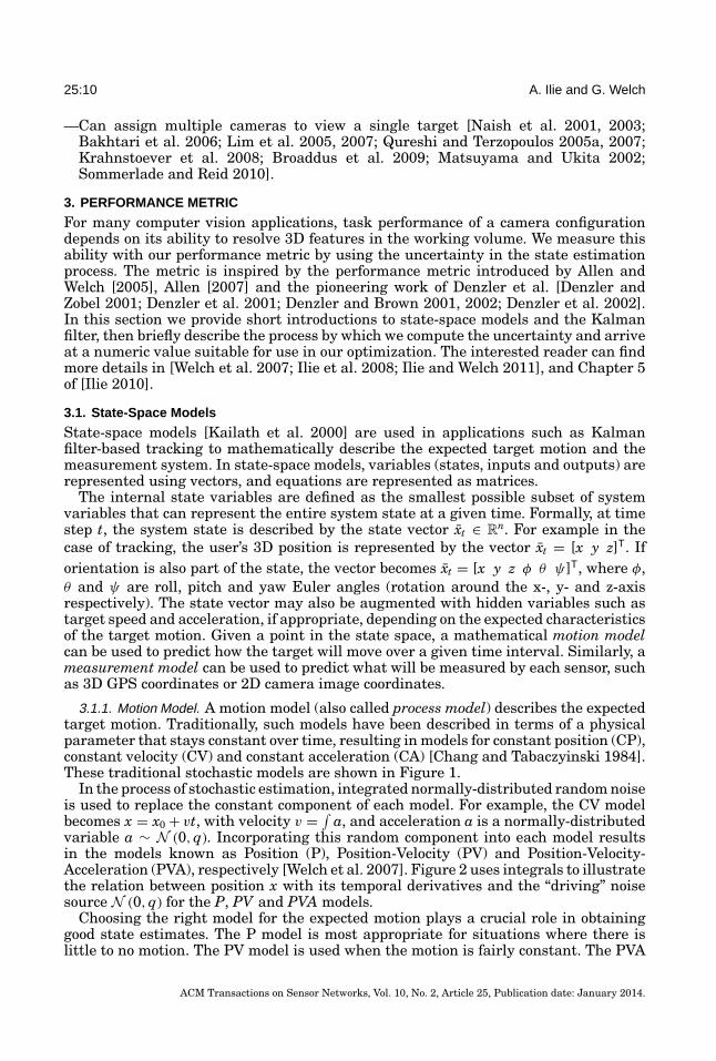
3.1.1. Motion Model. A motion model (also called process model) describes the expectedtarget motion. Traditionally, such models have been described in terms of a physicalparameter that stays constant over time, resulting in models for constant position (CP),constant velocity (CV) and constant acceleration (CA) [Chang and Tabaczyinski 1984].These traditional stochastic models are shown in Figure 1.
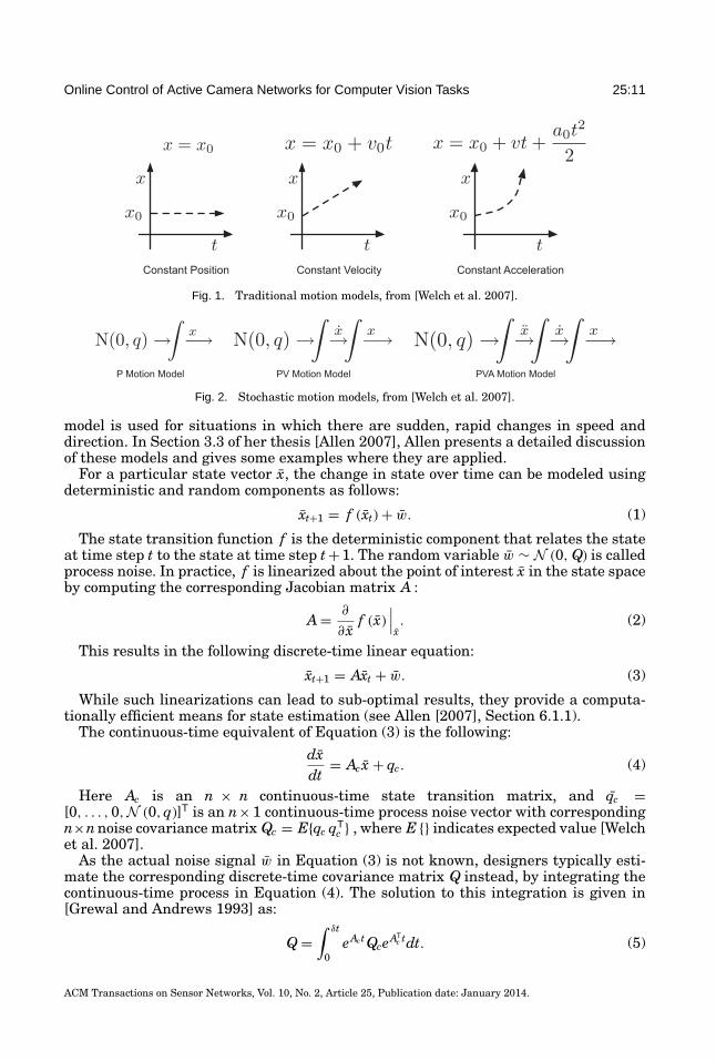
In the process of stochastic estimation, integrated normally-distributed random noiseis used to replace the constant component of each model. For example, the CV modelbecomes x = x0 + vt, with velocity v = ∫
a, and acceleration a is a normally-distributedvariable a ∼ N (0, q). Incorporating this random component into each model resultsin the models known as Position (P), Position-Velocity (PV) and Position-Velocity-Acceleration (PVA), respectively [Welch et al. 2007]. Figure 2 uses integrals to illustratethe relation between position x with its temporal derivatives and the “driving” noisesource N (0, q) for the P, PV and PVA models.
Choosing the right model for the expected motion plays a crucial role in obtaininggood state estimates. The P model is most appropriate for situations where there islittle to no motion. The PV model is used when the motion is fairly constant. The PVA
ACM Transactions on Sensor Networks, Vol. 10, No. 2, Article 25, Publication date: January 2014.
Online Control of Active Camera Networks for Computer Vision Tasks 25:11
Fig. 1. Traditional motion models, from [Welch et al. 2007].
Fig. 2. Stochastic motion models, from [Welch et al. 2007].
model is used for situations in which there are sudden, rapid changes in speed anddirection. In Section 3.3 of her thesis [Allen 2007], Allen presents a detailed discussionof these models and gives some examples where they are applied.
For a particular state vector x, the change in state over time can be modeled usingdeterministic and random components as follows:
xt+1 = f (xt) + w. (1)
The state transition function f is the deterministic component that relates the stateat time step t to the state at time step t + 1. The random variable w ∼ N (0, Q) is calledprocess noise. In practice, f is linearized about the point of interest x in the state spaceby computing the corresponding Jacobian matrix A :
A = ∂
∂ xf (x)
∣∣∣x. (2)
This results in the following discrete-time linear equation:
xt+1 = Axt + w. (3)
While such linearizations can lead to sub-optimal results, they provide a computa-tionally efficient means for state estimation (see Allen [2007], Section 6.1.1).
The continuous-time equivalent of Equation (3) is the following:
dxdt
= Acx + qc. (4)
Here Ac is an n × n continuous-time state transition matrix, and qc =[0, . . . , 0,N (0, q)]T is an n× 1 continuous-time process noise vector with correspondingn×n noise covariance matrix Qc = E{qc qT
c } , where E {} indicates expected value [Welchet al. 2007].
As the actual noise signal w in Equation (3) is not known, designers typically esti-mate the corresponding discrete-time covariance matrix Q instead, by integrating thecontinuous-time process in Equation (4). The solution to this integration is given in[Grewal and Andrews 1993] as:
Q =∫ δt
0eAct QceAT
c tdt. (5)
ACM Transactions on Sensor Networks, Vol. 10, No. 2, Article 25, Publication date: January 2014.
25:12 A. Ilie and G. Welch
Table I. Parameters for the P, PV and PVA Models
Model x Ac Qc Q
P [x][
0] [
q]
[q δt]
PV
[x_x
] [0 10 0
] [0 00 q
] [q δt3
3 q δt2
2
q δt2
2 q δt
]
PVA
⎡⎢⎣ x
_xx
⎤⎥⎦
⎡⎢⎣ 0 1 0
0 0 10 0 0
⎤⎥⎦
⎡⎢⎣ 0 0 0
0 0 00 0 q
⎤⎥⎦
⎡⎢⎣
q δt5
20 q δt4
8 q δt3
6
q δt4
8 q δt3
3 q δt2
2
q δt3
6 q δt2
2 q δt
⎤⎥⎦
Source: [Welch et al. 2007].
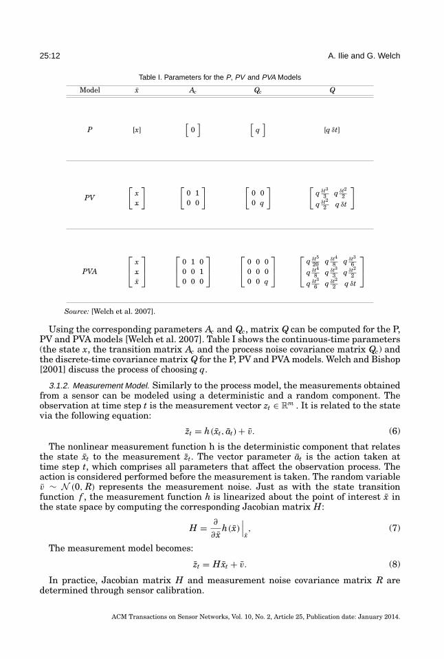
Using the corresponding parameters Ac and Qc, matrix Q can be computed for the P,PV and PVA models [Welch et al. 2007]. Table I shows the continuous-time parameters(the state x, the transition matrix Ac and the process noise covariance matrix Qc) andthe discrete-time covariance matrix Q for the P, PV and PVA models. Welch and Bishop[2001] discuss the process of choosing q.
3.1.2. Measurement Model. Similarly to the process model, the measurements obtainedfrom a sensor can be modeled using a deterministic and a random component. Theobservation at time step t is the measurement vector zt ∈ R
m . It is related to the statevia the following equation:
zt = h (xt, at) + v. (6)
The nonlinear measurement function h is the deterministic component that relatesthe state xt to the measurement zt. The vector parameter at is the action taken attime step t, which comprises all parameters that affect the observation process. Theaction is considered performed before the measurement is taken. The random variablev ∼ N (0, R) represents the measurement noise. Just as with the state transitionfunction f , the measurement function h is linearized about the point of interest x inthe state space by computing the corresponding Jacobian matrix H:
H = ∂
∂ xh (x)
∣∣∣x, (7)
The measurement model becomes:
zt = Hxt + v. (8)
In practice, Jacobian matrix H and measurement noise covariance matrix R aredetermined through sensor calibration.
ACM Transactions on Sensor Networks, Vol. 10, No. 2, Article 25, Publication date: January 2014.
Online Control of Active Camera Networks for Computer Vision Tasks 25:13
The actual noise signal v is not known or even estimated. Instead, designers typi-cally estimate the corresponding noise covariance matrix R, and use it to weight themeasurements and to estimate the state uncertainty.
State-space models allow taking into account measurements from multiple, heteroge-neous sensors. Allen describes such a system in her thesis (Allen [2007], Section 5.2.3).In Section 6, we present experimental evaluations using a hybrid system that takesmeasurements from multiple cameras and GPS sensors.
In the case of a GPS sensor, the measurement function h transforms a 3D point(latitude, longitude, altitude) into a local 3D coordinate system (x, y, z) used for trackingor 3D reconstruction. This transformation is a 3 × 3 linear transform H that can beused directly in Equation (8).
In the case of cameras, the measurement function h is embodied by the camera’sprojection matrix Proj, which projects a homogeneous 3D point [x y z 1]T to a homo-geneous 2D image pixel [ u′ v′ 1 ]T as follows:
⎡⎣ u
v
w
⎤⎦ = Proj
⎡⎢⎢⎣
xyz1
⎤⎥⎥⎦ (9)
u′ = u/w (10)v′ = v/w. (11)
The projection matrix Proj is typically determined through a geometric calibrationprocess like the one in Zhang [1999]. One common way to define matrix Proj is asfollows:
Proj = K[Rot|Tr
]. (12)
The 3×3 rotation matrix Rot and the 3×1 translation vector Tr represent the cameraextrinsic parameters, and specify the transform between the world coordinate systemand the camera’s coordinate system. The 3 × 4 matrix [Rot|Tr] is the concatenationof matrix Rot and vector Tr. The intrinsic parameters are represented by matrix K, a3 × 3 matrix of the form:
K =⎡⎣ fx s cx
0 fy cy
0 0 1
⎤⎦ . (13)
fx and fy are the camera focal lengths, measured in pixels, in the x and y directions.s is the skew, typically zero for cameras with square pixels. cx and cy are the coordinatesof the image center in pixels.
Since the camera measurement process embodied by the computation of u′ and v′ isnot linear, the following Jacobian is used in Equation (8).
H =
⎡⎢⎢⎣
∂u′
∂x∂u′
∂y∂u′
∂z∂v′
∂x∂v′
∂y∂v′
∂z
⎤⎥⎥⎦ . (14)
The measurement model is where some performance factors are integrated into themetric. The camera field of view and image resolution are integrated into the JacobianH via the camera projection model. Noise due to focus, mechanical camera components,and target distance is added into the noise covariance matrix R. The interested readeris referred to Section 5.4 of Ilie [2010] for more details.
ACM Transactions on Sensor Networks, Vol. 10, No. 2, Article 25, Publication date: January 2014.
25:14 A. Ilie and G. Welch
3.2. The Kalman Filter
The Kalman Filter [Welch and Bishop 2001] is a stochastic estimator for the instanta-neous state of a dynamic system that has been used both for tracking and for motionmodeling [Krahnstoever et al. 2001]. It can also be used as a tool for performance anal-ysis [Grewal and Andrews 1993] when actual measurements (real or simulated) areavailable. This section provides a brief introduction.
3.2.1. Equations. The Kalman filter consists of a set of mathematical equations thatimplement a predictor-corrector type estimator. Its equations can be described usingmatrices A, H, Q and R defined in the state-space models in Section 3.1, and the initialstate covariance P0. The equations for the predict and correct steps are as follows.
(1) Time Update (Predict Step).—Project state ahead:
x−t = f (xt−1, t − 1) . (15)
x−t ∈ R
n is the a priori state estimate at time step t, xt−1 ∈ Rn is the a posteriori state
estimate at time step t − 1, given measurement ¯zt−1, and f is the state transitionfunction.—Project error covariance ahead:
P−t = At Pt−1 AT
t + Q. (16)At is the Jacobian matrix of partial derivatives of the state transition function fwith respect to x at time step t.
(2) Measurement Update (Correct Step) – can only be performed if a measurement isavailable.—Compute Kalman gain:
Kt = P−t HT
t
(Ht P−
t HTt + R
)−1. (17)
Ht is the Jacobian matrix of partial derivatives of h with respect to x at time step t.Since h is a function of the selected action at, both Ht and Kt are functions of at.—Update state estimate with measurement zt:
x+t = x−
t + Kt(zt − h
(x−
t , at))
. (18)The expression Kt(zt − h(x−
t , at)) is called innovation, and quantifies the change instate over a single time step.—Update error covariance:
P+t = (I − Kt Ht) P−
t . (19)
Note that the a posteriori state covariance P+t does not depend on the measurement
zt. This allows evaluation of P+t over time in absence of measurements.
3.2.2. Sequential Evaluation. The sequential Kalman filter is a sequential evaluationmethod for the Kalman filter. The time update (predict) phase is identical to the onein the standard Kalman filter. The sequential evaluation takes place in the measure-ment update (correct) phase. Each sensor s = 1 . . . c is given its own subfilter. Theestimate x−
t , P−t from the predict phase becomes the a priori state estimate for the first
subfilter:
x−(1)t = x−
t (20)
P−(1)t = P−
t . (21)
Each sensor s incorporates its measurement zt(s), as in Equation (18):
x+(s)t = x−(s)
t + K(s)t
(zt
(s) − h(s)(x−(s)t , at
(s))). (22)
ACM Transactions on Sensor Networks, Vol. 10, No. 2, Article 25, Publication date: January 2014.
Online Control of Active Camera Networks for Computer Vision Tasks 25:15
The output state x+(s)t of each subfilter becomes the input state x−(s+1)
t for the nextsubfilter:
x−(s+1)t = x+(s)
t . (23)
Equations (22) and (23) can be aggregated into a single expression for the entire setof c subfilters:
x+(c)t = x−(1)
t +c∑
s=1
K(s)t
(zt
(s) − h(s)(x−(s)t , at
(s))). (24)
Let C(s)t be the contribution to the error covariance of each sensor s at time step t,
computed as:
C(s)t = I − K(s)
t H(s)t . (25)
The error covariance can be updated with the contribution C(s)t , as in Equation (19):
P+(s)t = C(s)
t P−(s)t . (26)
The output covariance P+(s)t of each subfilter becomes the input covariance P−(s+1)
tfor the next subfilter:
P−(s+1)t = P+(s)
t . (27)
Equations (26) and (27) can be aggregated into a single expression for the entire setof c subfilters:
P+(c)t =
c∏s=1
C(s)t P−(1)
t . (28)
If a sensor does not generate a measurement during a particular time step, thesequential Kalman filter allows simply skipping incorporating its contribution intoEquations (24) and (28). However, the contribution C(s)
t of each sensor s at time step tdepends on the a priori covariance of subfilter s, so the final a posteriori state x+
t = x+(c)t
and covariance P+t = P+(c)
t depend on the order in which the subfilters are evaluated.In practice, the effects of ordering are usually ignored.
3.3. Estimating and Predicting Performance
We define the performance of a camera configuration as its ability to resolve featuresin the working volume, and measure it using the uncertainty in the state estimationprocess. Uncertainty in the state x can be measured using the error covariance P+
tcomputed in the Kalman filter Equation (19).
In Ilie et al. [2008], we introduced the concept of surrogate models to allow evaluationof the metric in state-space only where needed: at a set of 3D points associated with eachROI. The metric values are aggregated over the state elements in the surrogate modelof each ROI, over each ROI group and over the entire environment. At all aggregationlevels, weights can be used to give more importance to a particular element. The choiceof surrogate model is paramount, as it allows incorporating task requirements into themetric. Section 5 presents a few examples.
Due to the dynamic nature of the events being captured and the characteristics ofthe active cameras used to capture images, time needs to be considered as a dimensionof the search space. Spatial aggregation of metric values over the environment for thecurrent camera configuration is not sufficient, and future camera configurations needto be evaluated as well. This results in the performance metric evaluating a plan: a
ACM Transactions on Sensor Networks, Vol. 10, No. 2, Article 25, Publication date: January 2014.
25:16 A. Ilie and G. Welch
temporal sequence of camera configurations up to a planning horizon. The difficulty isthat at each time instant a camera’s measurement can be successful or unsuccessful,depending on whether the ROI whose position is being measured is visible or not.Denzler et al. [2002] introduced a way to deal with visibility at each step. Deutsch et al.[2004] extended this approach to multiple steps into the future using a visibility tree,and then sped up the evaluation by linearizing the tree and extended the approach tomultiple cameras using a sequential Kalman filter in Deutsch et al. [2006]. We employa similar approach, but use a norm of the error covariance P+
t instead of entropy as ourperformance metric, and a different method to aggregate it over space and time. As themetric measures the uncertainty in the state, when comparing camera configurationssmaller values are better.
Our metric computation works in tandem with the Kalman filter that is used toestimate the ROI trajectories. At each time instant, the filter incorporates the lat-est measurements from cameras and other sensors, and saves the current estimate(x−
0 , P−0 ). This estimate is the starting point for all metric evaluations. To evaluate a
camera plan, we repeatedly perform sequential evaluations of the Kalman filter equa-tions, stepping forward in time, while using process models to predict ROI trajectoriesand updating the measurement models with the corresponding planned camera pa-rameters. When looking into the future, no actual measurements zt are available attime t, but estimated measurements zt = h(x−
t , at) can be used instead. Substituting ztfor zt results in zero innovation. Equation (18) becomes simply:
x+t = x−
t . (29)
At each time step, a camera measurement can be successful or not, depending ona variety of factors such as visibility, surface orientation, etc. If the measurementis assumed successful, the a posteriori state error covariance P+
t is computed as inEquation (19). If the measurement is assumed unsuccessful, the measurement updatestep cannot be performed, and P+
t = P−t . The two outcomes can be characterized by
two distributions with the same mean x+t and covariances P+
t and P−t . Given the
probability that a measurement is successful ms, these distributions can be consideredas components of a Gaussian mixture M [Deutsch et al. 2006]:
M = ms · N (x+
t , P+t
) + (1 − ms) · N (x+
t , P−t
). (30)
The covariance of the Gaussian mixture M is:
P+′t = ms · P+
t + (1 − ms) · P−t = (I − ms · Kt Ht) P−
t (31)
Since the two distributions have the same mean x+t , M is unimodal and can be ap-
proximated by a new Gaussian distribution M′(x+t , P+′
t ), as shown in Deutsch et al.[2006]. It follows that in order to incorporate the outcome of an observation, one simplyhas to compute the success probability and replace the computation of the a poste-riori error covariance in Equation (19) in the Kalman correct step with the one inEquation (31). The measurement success probability ms is where performance factorsthat affect visibility (such as occlusions and incidence angle) are integrated into themetric. The interested reader is referred to Section 5.4 of [Ilie 2010] for more details.
To aggregate over time, Deutsch et al. [2004, 2006] propose simply using the entropyvalue at the horizon. However, this value is very sensitive to the camera configurationsand ROI positions during the last few time steps before the horizon. For example,when an ROI is occluded in camera view, the uncertainty increases to reflect theabsence of measurements. Depending on the circumstances, such an increase duringthe last time steps before the horizon could end up penalizing plans that perform wellduring previous time steps. Conversely, a plan where the cameras become unoccludedduring the last time steps before the horizon can end up favored over a plan that
ACM Transactions on Sensor Networks, Vol. 10, No. 2, Article 25, Publication date: January 2014.
Online Control of Active Camera Networks for Computer Vision Tasks 25:17
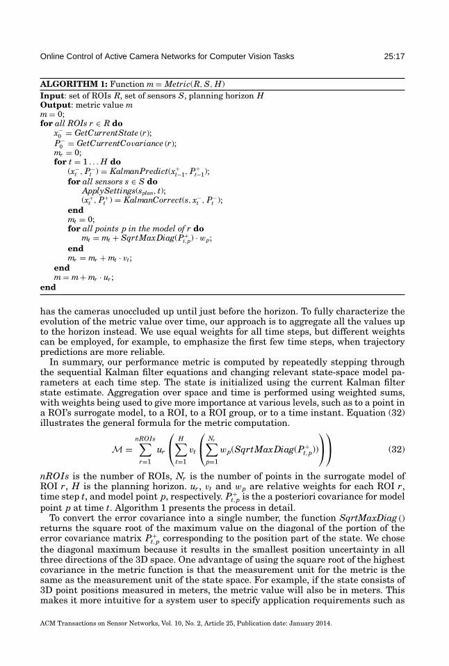
ALGORITHM 1: Function m = Metric(R, S, H)Input: set of ROIs R, set of sensors S, planning horizon HOutput: metric value mm = 0;for all ROIs r ∈ R do
x−0 = GetCurrentState (r);
P−0 = GetCurrentCovariance (r);
mr = 0;for t = 1 . . . H do
(x−t , P−
t ) = KalmanPredict(x+t−1, P+
t−1);for all sensors s ∈ S do
ApplySettings(splan, t);(x+
t , P+t ) = KalmanCorrect(s, x−
t , P−t );
endmt = 0;for all points p in the model of r do
mt = mt + SqrtMaxDiag(P+t,p) · wp;
endmr = mr + mt · vt;
endm = m+ mr · ur ;
end
has the cameras unoccluded up until just before the horizon. To fully characterize theevolution of the metric value over time, our approach is to aggregate all the values upto the horizon instead. We use equal weights for all time steps, but different weightscan be employed, for example, to emphasize the first few time steps, when trajectorypredictions are more reliable.
In summary, our performance metric is computed by repeatedly stepping throughthe sequential Kalman filter equations and changing relevant state-space model pa-rameters at each time step. The state is initialized using the current Kalman filterstate estimate. Aggregation over space and time is performed using weighted sums,with weights being used to give more importance at various levels, such as to a point ina ROI’s surrogate model, to a ROI, to a ROI group, or to a time instant. Equation (32)illustrates the general formula for the metric computation.
M =nROIs∑
r=1
ur
⎛⎝ H∑
t=1
vt
⎛⎝ Nr∑
p=1
wp(SqrtMaxDiag(P+t,p))
⎞⎠
⎞⎠ (32)
nROIs is the number of ROIs, Nr is the number of points in the surrogate model ofROI r, H is the planning horizon. ur, vt and wp are relative weights for each ROI r,time step t, and model point p, respectively. P+
t,p is the a posteriori covariance for modelpoint p at time t. Algorithm 1 presents the process in detail.
To convert the error covariance into a single number, the function SqrtMaxDiag ()returns the square root of the maximum value on the diagonal of the portion of theerror covariance matrix P+
t,p corresponding to the position part of the state. We chosethe diagonal maximum because it results in the smallest position uncertainty in allthree directions of the 3D space. One advantage of using the square root of the highestcovariance in the metric function is that the measurement unit for the metric is thesame as the measurement unit of the state space. For example, if the state consists of3D point positions measured in meters, the metric value will also be in meters. Thismakes it more intuitive for a system user to specify application requirements such as
ACM Transactions on Sensor Networks, Vol. 10, No. 2, Article 25, Publication date: January 2014.
25:18 A. Ilie and G. Welch
the desired maximum error in a particular area where important events take place.Entropy can also be used to convert the error covariance into a single number, but it ismore expensive to compute, and does not have the same real-world units as the squareroot of the diagonal maximum.
The interested reader is referred to Chapter 5 of Ilie [2010] for a detailed discussionon how we arrived at our performance metric, how it differs from previous approaches,and how it incorporates quality factors known to influence the performance of cameraconfigurations.
4. CONTROL METHOD
We define optimization in active camera control as the exploration of the space ofpossible solutions in search for the best solution as evaluated by the performancemetric: the minimum state uncertainty. In [Ilie 2010], we showed that exhaustivelyexploring the space of combinations of camera pan, tilt and zoom settings is intractable,even when applying heuristics to reduce the search space size. Instead, we explorethe space of camera-ROI assignments, and compute the best settings correspondingto each assignment using geometric reasoning: the best results are usually obtainedwhen the ROI trajectories are enclosed in the camera fields of view as tightly aspossible (see Section 4.4). Evaluating all possible combinations of plans for all camerasis intractable as well, but this search space features better opportunities to reduce itssize. We performed a careful analysis of the search space complexity, revealing multipleheuristics that reduce the search space size, and conducted experiments using ourmetric to evaluate them. While necessarily limited in scope, the experiments confirmedthat the heuristics were performing as expected. The interested reader is referred toChapter 4 of Ilie [2010] for details on how and why we chose the specific set of heuristicsin this section to reduce the size of the search space and ensure real-time performance.
During our analysis of the search space, we found that using proximity to decomposethe optimization problem into subproblems and solving each subproblem indepen-dently was the heuristic most effective at reducing the search space size. As a result,our camera control method consists of two components: centralized global assignmentand distributed local planning. The global assignment component groups ROIs intoagencies based on proximity to each other and assigns the appropriate cameras toeach agency. The local planning component is run at the level of each agency, andis responsible for finding the best plans for all the cameras assigned to that agency.The main advantage this strategy offers is that the subproblems associated with eachagency can be solved independently, in parallel. Another advantage is the opportunityto run the two components of our approach at different frequencies: for example, theglobal assignment component can be run once every N cycles, while the local planningcomponent can be run once per cycle at the level of each agency.
We perform a complete optimization during a planning cycle. For simplicity, andwithout loss of generality, we set the duration of a planning cycle to 1 second. Ourcurrent implementation, although not parallelized, still runs online, in real time (acomplete optimization per second). During each cycle, the optimization process firstpredicts the ROI trajectories up to the planning horizon, then uses them to constructand evaluate a number of candidate plans for each camera. A plan consists of a numberof planning steps, which in turn consist of a transition (during which the camerachanges its settings) and a dwell (during which the camera captures, with constantsettings). Candidate plans differ in the number and duration of planning steps up tothe planing horizon. We set the planning horizon to the minimum between a predefinednumber of seconds (set to ensure real-time performance) and the duration of the longestpossible camera capture, given the camera positions and capabilities and the predictedROI trajectories.
ACM Transactions on Sensor Networks, Vol. 10, No. 2, Article 25, Publication date: January 2014.
Online Control of Active Camera Networks for Computer Vision Tasks 25:19
4.1. Notation
Before presenting the algorithms that comprise our method, we introduce a few no-tation elements. We use standard sets notation: {. . .} is a set, ∅ is the empty set, ⊂represents a subset, ∈ represents membership, ≡ represents equality, = representsinequality, \ represents set difference, ∪ represents set union, and ∩ represents setintersection. Sets are denoted by capital letters like A, C, PS, R, R′ and set membersby small letters like a, c, p, r. A set member can be selected by its number. For example,C [n] is the n-th camera in set C.
Additionally, we use several variables, including the following:
—a plan P is denoted as a set of configurations over time, to which standard setoperations can be applied,
—P [start . . . stop] is plan P between times start and stop,—Pa is the plan for all cameras in agency a, and Pa,c is the plan for camera c in agency
a,—a.Current Plan is the current plan for agency a,—r.T rajectory [t] represents the surrogate model of ROI r at time t, from which points
can be selected, the top and bottom points in particular,—Ra is the set of ROIs in agency a,—Ca is the set of cameras assigned to agency a,—Cavail. is the set of available cameras,—c.Useful is a Boolean variable that specifies whether a camera c has been designated
as useful or not,—c.TransitionDuration and c.UninterruptibleDwellDuration are the transition and un-
interruptible dwell durations for camera c,—c.AspectRatio is the aspect ratio of camera c,—c.Choices is the set of capture choices (start time and duration) for camera c.
4.2. Global Assignment
The global assignment component accomplishes two tasks: grouping ROIs into agenciesand assigning cameras to each agency. We create agencies by clustering together ROIsthat are close to each other and predicted to be heading in similar directions. We usepredicted trajectories to cluster the ROIs into a minimum number of non-overlappingclusters of a given maximum diameter.
Standard clustering algorithms such as k-means ([Tan et al. 2005], Chapter 8) arenot immediately applicable, because the ROI trajectories are dynamic. Additionally,the membership of all ROI clusters needs to exhibit hysteresis to help keep the assign-ments stable. When an agency’s ROI membership changes, all cameras assigned to itneed to reevaluate their current plans. Since available cameras currently assigned toother agencies might contribute more to the modified agency, their possible contribu-tions need to be evaluated as well. If these evaluations result in changes in plans orassignments, cameras may need to transition, and end up spending less time captur-ing, which usually results in worse performance. To accommodate these requirements,we use a proximity-based minimal change heuristic, consisting of three steps.
(1) Assign each unassigned ROI to the agency closest to it if the agency would notbecome too large; form new agencies for remaining isolated ROIs.
(2) If any agency has become too large spatially, iteratively remove the ROI furthestfrom all other ROIs from it until the agency becomes small enough.
(3) If any two agencies are close enough to each other, merge them into a single agency.
Algorithm 2 presents the process in detail.
ACM Transactions on Sensor Networks, Vol. 10, No. 2, Article 25, Publication date: January 2014.
25:20 A. Ilie and G. Welch
ALGORITHM 2: Function A = ROIClustering(D, H, R, A)Input: cluster diameter D, horizon H, ROI set R, agencies set AOutput: agencies set APredictROIT rajectories (T , H);for all unassigned ROIs r ∈ R do
dmin = D;for all agencies a ∈ A do
d = Distance (r, a, H);if d < dmin then
Ra = Ra ∪ {r};dmin = d;amin = a;
endendif dmin ≡ D then
a = CreateAgency ();A = A∪ {a};
endelse
a = aminendRa = Ra ∪ {r}
endfor all agencies a ∈ A do
repeat{r1, r2} = MostDistant2ROIs (Ra, H);if Distance (r1, r2, H) > D then
R′ = Ra\ {r1, r2};if Distance (r1, R′, H) > Distance (r2, R′, H) then
r = r1endelse
r = r2endRa = Ra\ {r};AddToClosestAgency (r, D, H, A);if Ra ≡ ∅ then
A = A\ {a}end
enduntil Distance (r1, r2, H) ≤ D;
endrepeat
{a1,a2} = Closest2Agencies (A);if Distance (a1, a2, H) ≤ D then
a = Merge (a1, a2);A = A\ {a1, a2} ∪ {a};
enduntil Distance (a1, a2, H) > D;
Once agencies are created, we use a greedy heuristic to assign cameras to eachagency, based on their potential contribution to it. Formal approaches such as linearprogramming are not easily applicable because they are not always guaranteed toprovide a solution if the overall problem is infeasible. Only available cameras aretaken into account. A camera is considered available if its state for the next planning
ACM Transactions on Sensor Networks, Vol. 10, No. 2, Article 25, Publication date: January 2014.
Online Control of Active Camera Networks for Computer Vision Tasks 25:21
cycle is the start of a transition or an occlusion. Additionally, a camera’s dwell can beinterrupted if it has lasted longer than a specified minimum duration. The heuristic isalso proximity-based: a camera-agency assignment is evaluated only if the camera isclose enough to the ROIs in the agency. Proximity is evaluated in function IsClose ()to only try assigning cameras to nearby agencies. The heuristic tries assigning eachavailable camera to all nearby agencies, searching for the camera-agency assignmentthat best improves the metric value for the agency. Improvement is measured usingthe ratio maf ter/mbef ore, and the best improvement bi corresponds to the smallest ratio. Theinitial value for bi is 1+ε, where ε is a very small number. If a camera does not improvethe metric for any agency, its settings are left unchanged for the duration of the currentcycle. The resulting plans are compared with plans obtained by prolonging the currentplans up to the planning horizon whenever possible, and the greedy assignments areonly applied if they perform better. Algorithm 3 presents the process in detail.
ALGORITHM 3: Function Pgreedy = GreedyAssignment(A, C, H)
Input: set of agencies A, set of cameras C, horizon HOutput: heuristic plan PaCavail. = FindAvailableAgents (C);Pcurrent = ∅;for all agencies a ∈ A do
for all cameras c ∈ Ca doPa = BuildPlan(c, a, 1, H, true);Pcurrent = Pcurrent ∪ Pa;
endendPgreedy = Pcurrent;for all cameras c ∈ Cavail. do
bi = 1 + ε;mbef ore = Metric(A, Pgreedy, H);c.Useful = f alse;for all cameras c ∈ Cavail. do
if ∼ IsClose (c, a, H) thencontinue
endPa = BuildPlan(c, a, 1, H, c.agency ≡ a);AddCameraToAgency (c, a, Pa);maf ter = Metric(A, Pgreedy ∪ {Pa} , H);RemoveCameraFromAgency (c, a);ic,a = maf ter/mbef ore;if ic,a ≤ bi then
bi = ic,a;abest = a;Pbest = Pa;c.Usef ul = true;
endendif c.Useful then
AddCameraToAgency (c, abest, Pbest);Pgreedy = Pgreedy ∪ Pbest;
endCavail. = Cavail.\ {c};
end
ACM Transactions on Sensor Networks, Vol. 10, No. 2, Article 25, Publication date: January 2014.
25:22 A. Ilie and G. Welch
The plans corresponding to each camera-agency assignment are generated heuristi-cally by assuming the worst-case scenario: the camera is repeatedly set to transition,then capture for as long as possible, with a field of view as wide as possible. While otherscenarios, in which the camera captures for shorter intervals, may result in better per-formance by using narrower fields of view, the goal of this heuristic is only to quicklyassess the potential contribution a camera can have to the capture of the ROIs in theagency it is being assigned to. The heuristic also takes into account predicted staticand dynamic occlusions, and plans transitions during occlusions whenever possible, inorder to minimize the time when the camera is not capturing. Static occlusions areprecomputed off-line for each camera. Dynamic occlusions are computed online, usingthe predicted ROI trajectories. Algorithm 4 presents the process in detail.
ALGORITHM 4: Function Pa = BuildPlan(c, a, start, stop, prolong)Input: camera c, agency a, planning start and stop times, bool prolongOutput: heuristic plan Pat = start;Pa = a.CurrentPlan;if prolong then
Pa = ProlongCurrentCapture (Pa);t = EndOfFirstCaptureTime (Pa);
endPa = Pa
[1 . . . t
];
while t < stop dotFoV = WidestFoVCaptureTime (c, a, t, stop);toccl = NextOcclusionStart (c, a, t, stop);e = min (tFoV , toccl);Pa [t . . . e] = ComputeSettings (c, a, t, e);if tFoV < toccl then
t = e;else
t = NextOcclusionEnd (c, a, t, stop) − c.T ransitionDuration;end
end
The number of assignments evaluated is nAgencies ·nCamsavail.. Note that the resultsof the assignment process are dependent on the order in which cameras are considered.If all possibilities were evaluated instead, the complexity would increase to nAgencies ·nCamsavail. (nCamsavail. + 1) /2, and a formula quadratic in nCamsavail. is often likely toresult in slower than real-time performance.
It is worth noting that two small changes in our global assignment algorithmmake it general enough to apply to camera selection as well. A scenario likely to beencountered in practice is that the camera infrastructure installed at a site might haveboth F fixed cameras and A active cameras, as well as a number D of devices to recordthe video streams coming from the cameras. If there are not enough devices to recordall the streams (D < A+ F), a modified assignment approach can be used to decidewhich streams to record. The changes would simply be to return after assigning Dcameras and to skip the planning of transitions and dwells for fixed cameras. Selectinga set of cameras to record would not preclude other algorithms that can run in realtime (such as tracking) from running using all camera streams, or from potentiallycontributing their input to our method.
ACM Transactions on Sensor Networks, Vol. 10, No. 2, Article 25, Publication date: January 2014.
Online Control of Active Camera Networks for Computer Vision Tasks 25:23
4.3. Local Planning
Local planning at the level of each agency is concerned with the locally-optimal captureof the ROIs in the agency. All cameras assigned to each agency capture all memberROIs, and no further camera-ROI assignment decisions are made at this level. Theplanning decisions made at this level are on when and for how long each camerashould dwell (capture), and when it should transition to a new configuration.
The current configuration of each camera, corresponding to the first step in a plan,is arguably the most important: configurations corresponding to subsequent steps arerevised during subsequent optimization cycles, when the planning method can takeadvantage of updated predictions of ROI trajectories. We take advantage of this andcall the resulting planning process myopic: exhaustive exploration of all possible dwelldurations is only done during the first planning step, and heuristic computations areused for subsequent steps up to the time horizon.
During each evaluation cycle, a decision is made whether to keep the current camerasettings or to transition to a new configuration. We reduce the search complexity byhaving the planning process be lazy: only making this decision for the first cycle ina planning step. Subsequent cycles will simply leave in place the result of the deci-sion made during the first cycle. The reasoning behind this heuristic is, again, thatthe predicted trajectories available during subsequent cycles are less precise, and theplanning process will get a chance to make a decision for each cycle when it becomesthe current cycle, and is provided with updated trajectory estimates.
The interested reader is referred to Chapter 4 of Ilie [2010] for a discussion onthe impact of myopic, lazy, and other planning heuristics on the size of the searchspace. While significantly reducing the search space, they can still sometimes resultin too many plans to evaluate for running in real time. We further reduce the numberof candidate plans by planning transitions during occlusions and limiting how manyplanning steps of minimum length can fit before the planning horizon. The heuristicemployed for completing plans beyond the first step is the same one used during globalassignment: function BuildPlan (), described in Algorithm 4.
Static occlusions do not depend on the camera parameters, so they are precomputedfor each camera in the variable c.Visib. and used to further reduce the number ofpossible plans in the ComputeStaticVisibilities () function. Other restrictions, such ashow many planning steps of minimum length can fit before the planning horizon, canbe taken into account as well in the FindChoices () function.
To achieve online, realtime control, the set of candidate plans can be sorted so thatthe most promising plans are evaluated first. One can use prior experimental obser-vations to derive criteria for quickly judging a plan’s potential without a costly metricevaluation.
While not a guarantee that the best plan would be chosen on time, we have foundthis combination of heuristics to closely approximate an exhaustive search. The finalresult of the planning heuristics is a set of candidate plans for each camera. All pos-sible combinations of candidate plans for all cameras are explored exhaustively usingbacktracking. Algorithm 5 presents the local planning procedure, Algorithm 6 detailsthe backtracking procedure, and Algorithm 7 shows a simple example of how the set ofchoices for the first planning step’s end time can be computed.
4.4. Computing Camera Settings
Once the start cycle and capture duration are decided for a planning step in a camera’splan, we use geometric reasoning to compute the corresponding camera pan, tilt andzoom values that ensure optimal coverage of all the ROIs in the agency the camera has
ACM Transactions on Sensor Networks, Vol. 10, No. 2, Article 25, Publication date: January 2014.
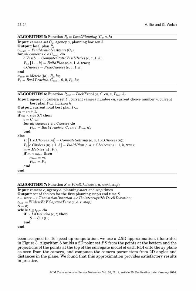
25:24 A. Ilie and G. Welch
ALGORITHM 5: Function Pa = LocalPlanning (Ca, a, h)Input: camera set Ca, agency a, planning horizon hOutput: local plan PaCavail. = FindAvailableAgents (Ca);for all cameras c ∈ Cavail. do
c.V isib. = ComputeStaticV isibilities (c, a, 1, h);Pa,c
[1 . . . h
] = BuildPlan(c, a, 1, h, true);c.Choices = FindChoices (c, a, 1, h);
endmbest = Metric ({a} , Pa, h);Pa = BackT rack (a, Cavail., 0, 0, Pa, h);
ALGORITHM 6: Function Pbest = BackT rack (a, C, cn, n, Pbest, h)Input: agency a, camera set C, current camera number cn, current choice number n, current
best plan Pbest, horizon hOutput: current local best plan Pbestcn = cn + 1;if cn < size (C) then
c = C [cn];for all choices i ∈ c.Choices do
Pbest = BackT rack (a, C, cn, i, Pbest, h);end
elsePa
[1, c.Choices (n)
] = ComputeSettings (c, a, 1, c.Choices (n));Pa
[c.Choices (n) + 1, h
] = BuildPlan(c, a, c.Choices (n) + 1, h, true);m = Metric ({a} , Pa);if m < mbest then
mbest = m;Pbest = Pa;
endend
ALGORITHM 7: Function S = FindChoices (c, a, start, stop)Input: camera c, agency a, planning start and stop timesOutput: set of choices for the first planning step’s end time St = start + c.T ransitionDuration+ c.UninterruptibleDwellDuration;tFoV = WidestFoV CaptureT ime (c, a, t, stop);S = ∅;while t ≤ tFoV do
if ∼ IsOccluded (c, t) thenS = S ∪ {t};
endend
been assigned to. To speed up computation, we use a 2.5D approximation, illustratedin Figure 3. Algorithm 8 builds a 2D point set PS from the points at the bottom and theprojections of the points at the top of the surrogate model of each ROI onto the xy planeas seen from the camera, and computes the camera parameters from 2D angles anddistances in the plane. We found that this approximation provides satisfactory resultsin practice.
ACM Transactions on Sensor Networks, Vol. 10, No. 2, Article 25, Publication date: January 2014.
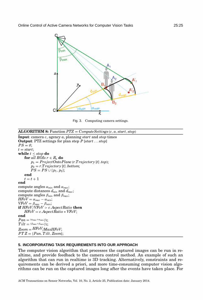
Online Control of Active Camera Networks for Computer Vision Tasks 25:25
Fig. 3. Computing camera settings.
ALGORITHM 8: Function PTZ = ComputeSettings (c, a, start, stop)Input: camera c, agency a, planning start and stop timesOutput: PTZ settings for plan step P [start . . . stop]PS = ∅;t = start;while t ≤ stop do
for all ROIs r ∈ Ra dop1 = ProjectOntoPlane (r.T rajectory [t] .top);p2 = r.T rajectory [t] .bottom;PS = PS ∪ {p1, p2};
endt = t + 1
endcompute angles αmin and αmax;compute distances dmin and dmax;compute angles βmin and βmax;HFoV = αmax − αmin;VFoV = βmax − βmin;if HFoV/VFoV > c.AspectRatio then
HFoV = c.AspectRatio ∗ VFoV;endPan = (αmax+αmin)/2;T ilt = (βmax+βmin)/2;Zoom = HFoV/MaxHFoV;PT Z = {Pan, T ilt, Zoom};
5. INCORPORATING TASK REQUIREMENTS INTO OUR APPROACH
The computer vision algorithm that processes the captured images can be run in re-altime, and provide feedback to the camera control method. An example of such analgorithm that can run in realtime is 3D tracking. Alternatively, constraints and re-quirements can be derived a priori, and more time-consuming computer vision algo-rithms can be run on the captured images long after the events have taken place. For
ACM Transactions on Sensor Networks, Vol. 10, No. 2, Article 25, Publication date: January 2014.
25:26 A. Ilie and G. Welch
example, 3D reconstruction algorithms can be time-consuming, but rigorously speci-fying their requirements allows the capture of images that can still guarantee goodresults even without real-time feedback. Many task requirements become easy andintuitive to incorporate into our method due to the performance metric being in state-space. In this section, we give a few examples of how common task requirements canbe incorporated, grouped by the application domain. The interested reader is referredto Chapters 5 and 6 of Ilie [2010] for a more detailed presentation of our performancemetric and camera control method, including a discussion on applying them to a varietyof tasks.
5.1. Tracking
The requirements of a tracking application are naturally expressed in state-space. Forexample, the user of a tracking system may specify the desired tracking accuracy fora particular region where events might be more important or more likely to happen,or for a particular ROI enclosing a person deemed more important. This importanceappears as a weight in the aggregation part of the metric function, and affects theoptimization process.
The state can be modeled as a single 3D point if the user is only interested in theROI’s position, or multiple points placed for example at the skeleton joints if the userdesires motion capture. Models can be augmented with local surface orientation if theuser wants to take into account self-occlusion. The state can also be reduced to 2D ifthe tracking system employs a ground plane assumption, in which case a single camerameasurement is sufficient to determine the ROI position at any time.
5.2. Surveillance
Surveillance tasks have very diverse goals. Here we give two examples of surveillancetasks and how they can be accommodated by our approach.
(1) Following a person or object throughout the environment: enclose the person orobject inside a ROI and set its importance higher than the importance of otherROIs. The camera control method will automatically follow the more importantROI and exhibit complex behaviors such as coordination and hand-offs betweencameras.
(2) Capturing images of people’s faces for biometric tasks: augment the surrogatemodel with points on the person’s face and the person’s movement and/or gazedirection, and incorporate the incidence angle into the metric computation as afactor in the probability of making a successful measurement ms in Equations (30)and (31). To ensure the capture of as many faces as possible, have a single successfulcapture drastically decrease the importance of the captured target’s ROI. This willresult in cameras capturing other faces that are comparably more uncertain. Astime passes, repeated captures of the same person’s face if still present in theenvironment can be ensured by having the importance of its ROI increase slowlyover time.
5.3. 3D Reconstruction
When the application is a 3D reconstruction method, surrogate models can be adjustedto better fit the requirements of the particular 3D reconstruction approach. We presenttwo examples.
(1) Surrogate models for stereo reconstruction could be augmented with local surfaceorientation, which can be included in an appropriate aggregation function that usesthe angle between the camera ray and the surface normal. The resulting metricwould give more weight to samples better suited for stereo matching. This change
ACM Transactions on Sensor Networks, Vol. 10, No. 2, Article 25, Publication date: January 2014.
Online Control of Active Camera Networks for Computer Vision Tasks 25:27
results in the metric giving preference to camera configurations that have beenshown to work better in stereo reconstruction: cameras placed relatively close toeach other and aimed in a similar direction.
(2) The default approach of minimizing the uncertainty in the 3D position of a numberof points gives good results in 3D volumetric reconstruction. However, a differentkind of surrogate model for volumetric 3D reconstruction could instead consist ofa medial axis-like representation: a set of 3D centroids and rays to the surface.The metric to be optimized could then be an aggregation of the uncertainties inthe length of the rays together with the ray lengths themselves, since volumetricapproaches typically seek a 3D model of minimum volume. Both approaches resultin the metric giving preference to camera configurations that have been shown towork better in volumetric reconstruction: cameras placed uniformly around a ROI,in an outside-looking-in arrangement.
5.4. New Targets
There are multiple ways of incorporating new persons or objects entering theenvironment.
(1) One approach is suggested by previous work in surveillance such as Krahnstoeveret al. [2008], and applies to enclosed environments with a limited number of entrypoints. In this case, previous approaches have scheduled cameras to periodicallysurvey the entry points for any potential new targets. A similar approach can bestraightforwardly applied to our method by having static ROIs enclose the entrypoints, and automatically creating new dynamic ROIs enclosing any new targetswhen they are detected entering the scene. Given appropriate surrogate models foreach ROI, the camera control method would automatically plan available camerasto both survey the static ROIs enclosing the entry points and to track the newlycreated dynamic ROIs.
(2) Another approach is introduced by Sommerlande and Reid [2008a]. They model theprobability of new targets entering the scene using a background Poisson process,and integrate the noise injected by the process into the performance metric fromDeutsch et al. [2006]. Since our performance metric is in many respects similar tothe one in Deutsch et al. [2006], this approach is easily applicable to it as well.
(3) A third approach is to have the state of new ROIs bootstrapped by input froman external system, for example GPS or a tracking system that uses a few staticcameras with wide fields of view to cover the entire scene. This is another areawhere state-space models demonstrate their usefulness: besides helping to acquirenew targets, measurements from these external devices can be incorporated intothe sequential evaluation process described in Section 3.2.2, and thus contributeto reducing the uncertainty in the state.
6. EXPERIMENTAL RESULTS
6.1. Simulation-Based Experimental Results
6.1.1. Experiment Setup. A training exercise was performed by members of the UnitedStates Marines Corp, and captured on-site at the Sarnoff Corporation in Princeton, NJ.The exercise participants’ trajectories were used to test how an implementation of ourmethod can control six PTZ cameras to observe six exercise participants.
The exercise scenario was for a squad of four Marines to patrol, cross a danger zonebetween two buildings, cordon and search a civilian, neutralize a sniper threat, andmove out to secure an area.
We used the game engine-based simulator from Taylor et al. [2007] to run multiplesimulations using the same input data. The simulator provides means of controlling
ACM Transactions on Sensor Networks, Vol. 10, No. 2, Article 25, Publication date: January 2014.
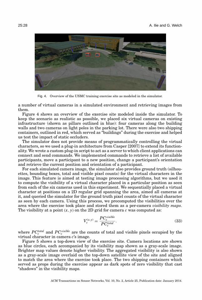
25:28 A. Ilie and G. Welch
Fig. 4. Overview of the USMC training exercise site as modeled in the simulator.
a number of virtual cameras in a simulated environment and retrieving images fromthem.
Figure 4 shows an overview of the exercise site modeled inside the simulator. Tokeep the scenario as realistic as possible, we placed six virtual cameras on existinginfrastructure (shown as pillars outlined in blue): four cameras along the buildingwalls and two cameras on light poles in the parking lot. There were also two shippingcontainers, outlined in red, which served as “buildings” during the exercise and helpedus test the impact of static occluders.
The simulator does not provide means of programmatically controlling the virtualcharacters, so we used a plug-in architecture from Casper [2007] to extend its function-ality. We wrote a custom plug-in script to act as a server to which client applications canconnect and send commands. We implemented commands to retrieve a list of availableparticipants, move a participant to a new position, change a participant’s orientationand retrieve the current position and orientation of a participant.
For each simulated camera image, the simulator also provides ground truth (silhou-ettes, bounding boxes, total and visible pixel counts) for the virtual characters in theimage. This feature is aimed at testing image processing algorithms, but we used itto compute the visibility of a virtual character placed in a particular position as seenfrom each of the six cameras used in this experiment. We sequentially placed a virtualcharacter at positions on a 2D regular grid spanning the area, aimed all cameras atit, and queried the simulator for the ground truth pixel counts of the virtual characteras seen by each camera. Using this process, we precomputed the visibilities over thearea where the exercise took place and stored them as a per-camera visibility maps.The visibility at a point (x, y) on the 2D grid for camera c was computed as:
V (x,y)c = PCvisible
c
PCtotalc
. (33)
where PCtotalc and PCvisible
c are the counts of total and visible pixels occupied by thevirtual character in camera c’s image.
Figure 5 shows a top-down view of the exercise site. Camera locations are shownas blue circles, each accompanied by its visibility map shown as a gray-scale image.Brighter map values denote higher visibility. The aggregated visibility is also shownas a gray-scale image overlaid on the top-down satellite view of the site and alignedto match the area where the exercise took place. The two shipping containers whichserved as props during the exercise appear as dark spots of zero visibility that cast“shadows” in the visibility maps.
ACM Transactions on Sensor Networks, Vol. 10, No. 2, Article 25, Publication date: January 2014.
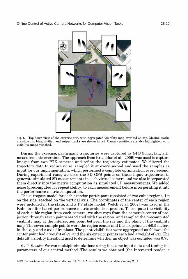
Online Control of Active Camera Networks for Computer Vision Tasks 25:29
Fig. 5. Top-down view of the exercise site, with aggregated visibility map overlaid on top. Marine tracksare shown in blue, civilian and sniper tracks are shown in red. Camera positions are also highlighted, withvisibility maps attached.
During the exercise, participant trajectories were captured as GPS (long., lat., alt.)measurements over time. The approach from Broaddus et al. [2009] was used to captureimages from two PTZ cameras and refine the trajectory estimates. We filtered thetrajectory data to reduce noise, sampled it at every second and used the samples asinput for our implementation, which performed a complete optimization every second.During experiment runs, we used the 3D GPS points on these input trajectories togenerate simulated 2D measurements in each virtual camera and we also incorporatedthem directly into the metric computation as simulated 3D measurements. We addednoise (precomputed for repeatability) to each measurement before incorporating it intothe performance metric computation.
The surrogate model for each exercise participant consisted of two cubic regions, 1mon the side, stacked on the vertical axis. The coordinates of the center of each regionwere included in the state, and a PV state model [Welch et al. 2007] was used in theKalman filter-based performance metric evaluation process. To compute the visibilityof each cubic region from each camera, we shot rays from the camera’s center of pro-jection through seven points associated with the region, and sampled the precomputedvisibility map at the intersection point between the ray and the plane of the visibilitymap. The seven sample points were the region center and the six points at ±0.5 metersin the x, y and z axis directions. The point visibilities were aggregated as follows: thecenter point had a weight of 1/2, and the six exterior points each had a weight of 1/12. Thedefault visibility threshold used to determine whether an object was occluded was 0.75.
6.1.2. Results. We ran multiple simulations using the same input data and tuning theparameters of our control method. The results we obtained (the interested reader is
ACM Transactions on Sensor Networks, Vol. 10, No. 2, Article 25, Publication date: January 2014.
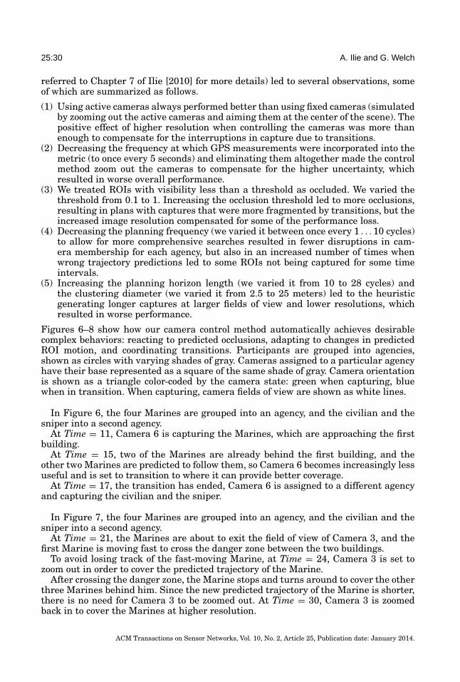
25:30 A. Ilie and G. Welch
referred to Chapter 7 of Ilie [2010] for more details) led to several observations, someof which are summarized as follows.
(1) Using active cameras always performed better than using fixed cameras (simulatedby zooming out the active cameras and aiming them at the center of the scene). Thepositive effect of higher resolution when controlling the cameras was more thanenough to compensate for the interruptions in capture due to transitions.
(2) Decreasing the frequency at which GPS measurements were incorporated into themetric (to once every 5 seconds) and eliminating them altogether made the controlmethod zoom out the cameras to compensate for the higher uncertainty, whichresulted in worse overall performance.
(3) We treated ROIs with visibility less than a threshold as occluded. We varied thethreshold from 0.1 to 1. Increasing the occlusion threshold led to more occlusions,resulting in plans with captures that were more fragmented by transitions, but theincreased image resolution compensated for some of the performance loss.
(4) Decreasing the planning frequency (we varied it between once every 1 . . . 10 cycles)to allow for more comprehensive searches resulted in fewer disruptions in cam-era membership for each agency, but also in an increased number of times whenwrong trajectory predictions led to some ROIs not being captured for some timeintervals.
(5) Increasing the planning horizon length (we varied it from 10 to 28 cycles) andthe clustering diameter (we varied it from 2.5 to 25 meters) led to the heuristicgenerating longer captures at larger fields of view and lower resolutions, whichresulted in worse performance.
Figures 6–8 show how our camera control method automatically achieves desirablecomplex behaviors: reacting to predicted occlusions, adapting to changes in predictedROI motion, and coordinating transitions. Participants are grouped into agencies,shown as circles with varying shades of gray. Cameras assigned to a particular agencyhave their base represented as a square of the same shade of gray. Camera orientationis shown as a triangle color-coded by the camera state: green when capturing, bluewhen in transition. When capturing, camera fields of view are shown as white lines.
In Figure 6, the four Marines are grouped into an agency, and the civilian and thesniper into a second agency.
At Time = 11, Camera 6 is capturing the Marines, which are approaching the firstbuilding.
At Time = 15, two of the Marines are already behind the first building, and theother two Marines are predicted to follow them, so Camera 6 becomes increasingly lessuseful and is set to transition to where it can provide better coverage.
At Time = 17, the transition has ended, Camera 6 is assigned to a different agencyand capturing the civilian and the sniper.
In Figure 7, the four Marines are grouped into an agency, and the civilian and thesniper into a second agency.
At Time = 21, the Marines are about to exit the field of view of Camera 3, and thefirst Marine is moving fast to cross the danger zone between the two buildings.
To avoid losing track of the fast-moving Marine, at Time = 24, Camera 3 is set tozoom out in order to cover the predicted trajectory of the Marine.
After crossing the danger zone, the Marine stops and turns around to cover the otherthree Marines behind him. Since the new predicted trajectory of the Marine is shorter,there is no need for Camera 3 to be zoomed out. At Time = 30, Camera 3 is zoomedback in to cover the Marines at higher resolution.
ACM Transactions on Sensor Networks, Vol. 10, No. 2, Article 25, Publication date: January 2014.
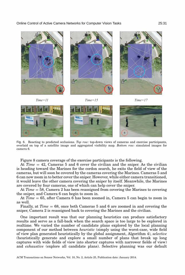
Online Control of Active Camera Networks for Computer Vision Tasks 25:31
Fig. 6. Reacting to predicted occlusions. Top row: top-down views of cameras and exercise participants,overlaid on top of a satellite image and aggregated visibility map. Bottom row: simulated images forcamera 6.
Figure 8 camera coverage of the exercise participants is the following.At Time = 42, Cameras 5 and 6 cover the civilian and the sniper. As the civilian
is heading toward the Marines for the cordon search, he exits the field of view of thecameras, but will soon be covered by the cameras covering the Marines. Cameras 5 and6 can now zoom in to better cover the sniper. However, while either camera transitioned,it would leave the other camera covering the sniper by itself. Meanwhile, the Marinesare covered by four cameras, one of which can help cover the sniper.
At Time = 58, Camera 2 has been reassigned from covering the Marines to coveringthe sniper, and Camera 6 can begin to zoom in.
At Time = 65, after Camera 6 has been zoomed in, Camera 5 can begin to zoom inas well.
Finally, at Time = 68, once both Cameras 5 and 6 are zoomed in and covering thesniper, Camera 2 is reassigned back to covering the Marines and the civilian.
One important result was that our planning heuristics can produce satisfactoryresults and serve as a fall-back when the search space is too large to be explored inrealtime. We varied the number of candidate plans explored by the local planningcomponent of our method between heuristic (simply using the worst-case, wide fieldof view plan generated heuristically by the global assignment, Algorithm 4), selective(heuristically generate and explore a small number of plans that break up longcaptures with wide fields of view into shorter captures with narrower fields of view)and exhaustive (explore all candidate plans). Selective planning was our default
ACM Transactions on Sensor Networks, Vol. 10, No. 2, Article 25, Publication date: January 2014.
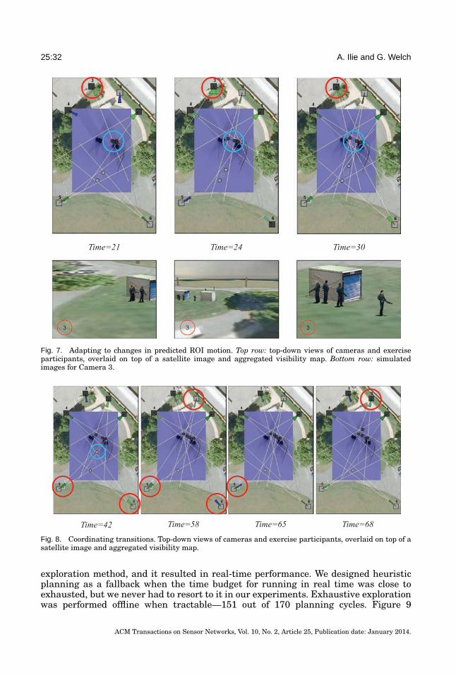
25:32 A. Ilie and G. Welch
Fig. 7. Adapting to changes in predicted ROI motion. Top row: top-down views of cameras and exerciseparticipants, overlaid on top of a satellite image and aggregated visibility map. Bottom row: simulatedimages for Camera 3.
Fig. 8. Coordinating transitions. Top-down views of cameras and exercise participants, overlaid on top of asatellite image and aggregated visibility map.
exploration method, and it resulted in real-time performance. We designed heuristicplanning as a fallback when the time budget for running in real time was close toexhausted, but we never had to resort to it in our experiments. Exhaustive explorationwas performed offline when tractable—151 out of 170 planning cycles. Figure 9
ACM Transactions on Sensor Networks, Vol. 10, No. 2, Article 25, Publication date: January 2014.
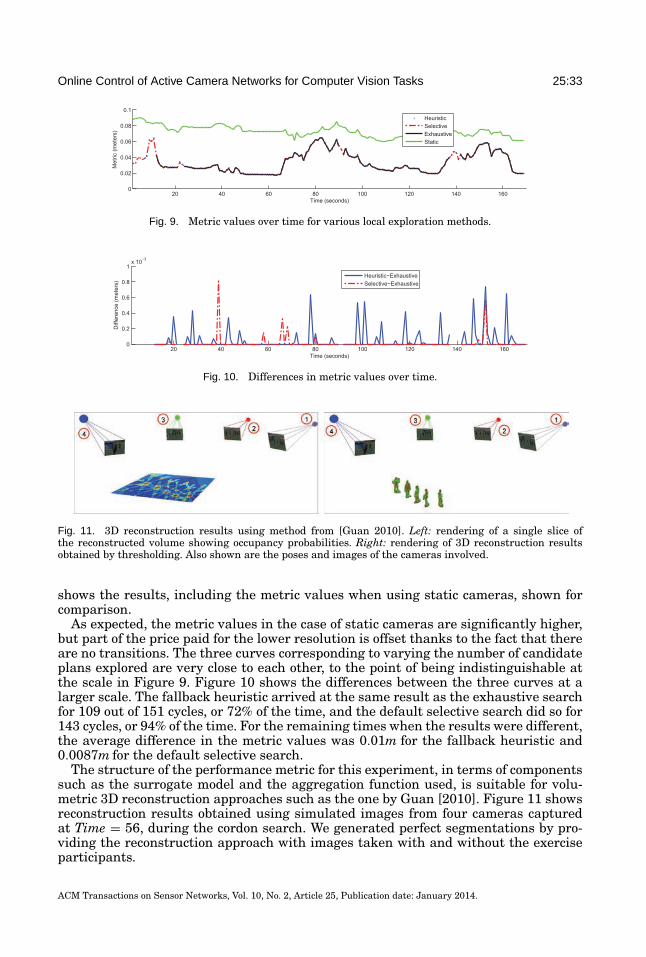
Online Control of Active Camera Networks for Computer Vision Tasks 25:33
Fig. 9. Metric values over time for various local exploration methods.
Fig. 10. Differences in metric values over time.
Fig. 11. 3D reconstruction results using method from [Guan 2010]. Left: rendering of a single slice ofthe reconstructed volume showing occupancy probabilities. Right: rendering of 3D reconstruction resultsobtained by thresholding. Also shown are the poses and images of the cameras involved.
shows the results, including the metric values when using static cameras, shown forcomparison.
As expected, the metric values in the case of static cameras are significantly higher,but part of the price paid for the lower resolution is offset thanks to the fact that thereare no transitions. The three curves corresponding to varying the number of candidateplans explored are very close to each other, to the point of being indistinguishable atthe scale in Figure 9. Figure 10 shows the differences between the three curves at alarger scale. The fallback heuristic arrived at the same result as the exhaustive searchfor 109 out of 151 cycles, or 72% of the time, and the default selective search did so for143 cycles, or 94% of the time. For the remaining times when the results were different,the average difference in the metric values was 0.01m for the fallback heuristic and0.0087m for the default selective search.
The structure of the performance metric for this experiment, in terms of componentssuch as the surrogate model and the aggregation function used, is suitable for volu-metric 3D reconstruction approaches such as the one by Guan [2010]. Figure 11 showsreconstruction results obtained using simulated images from four cameras capturedat Time = 56, during the cordon search. We generated perfect segmentations by pro-viding the reconstruction approach with images taken with and without the exerciseparticipants.
ACM Transactions on Sensor Networks, Vol. 10, No. 2, Article 25, Publication date: January 2014.
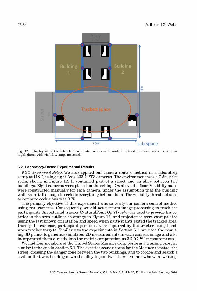
25:34 A. Ilie and G. Welch
Fig. 12. The layout of the lab where we tested our camera control method. Camera positions are alsohighlighted, with visibility maps attached.
6.2. Laboratory-Based Experimental Results
6.2.1. Experiment Setup. We also applied our camera control method in a laboratorysetup at UNC, using eight Axis 233D PTZ cameras. The environment was a 7.5m× 9mroom, shown in Figure 12. It contained part of a street and an alley between twobuildings. Eight cameras were placed on the ceiling, 7mabove the floor. Visibility mapswere constructed manually for each camera, under the assumption that the buildingwalls were tall enough to occlude everything behind them. The visibility threshold usedto compute occlusions was 0.75.
The primary objective of this experiment was to verify our camera control methodusing real cameras. Consequently, we did not perform image processing to track theparticipants. An external tracker (NaturalPoint OptiTrack) was used to provide trajec-tories in the area outlined in orange in Figure 12, and trajectories were extrapolatedusing the last known orientation and speed when participants exited the tracked area.During the exercise, participant positions were captured by the tracker using head-worn tracker targets. Similarly to the experiments in Section 6.1, we used the result-ing 3D points to generate simulated 2D measurements in each camera image and alsoincorporated them directly into the metric computation as 3D “GPS” measurements.
We had four members of the United States Marines Corp perform a training exercisesimilar to the one in Section 6.1. The exercise scenario was for the Marines to patrol thestreet, crossing the danger zone between the two buildings, and to cordon and search acivilian that was heading down the alley to join two other civilians who were waiting.
ACM Transactions on Sensor Networks, Vol. 10, No. 2, Article 25, Publication date: January 2014.
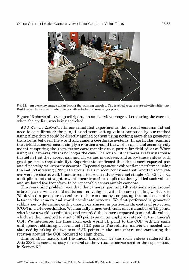
Online Control of Active Camera Networks for Computer Vision Tasks 25:35
Fig. 13. An overview image taken during the training exercise. The tracked area is marked with white tape.Building walls were simulated using cloth attached to waist-high posts.
Figure 13 shows all seven participants in an overview image taken during the exercisewhen the civilian was being searched.
6.2.2. Camera Calibration. In our simulated experiments, the virtual cameras did notneed to be calibrated: the pan, tilt and zoom setting values computed by our methodusing Algorithm 8 could be directly applied to them using nothing more than geometrictransforms between the world and camera coordinate systems. In particular, panningthe virtual cameras meant simply a rotation around the world z axis, and zooming onlymeant computing the zoom factor corresponding to a particular field of view. Whenusing real cameras, this is no longer the case. The Axis 233D cameras are fairly sophis-ticated in that they accept pan and tilt values in degrees, and apply these values withgreat precision (repeatability). Experiments confirmed that the camera-reported panand tilt setting values were accurate. Repeated geometric calibrations performed usingthe method in Zhang [1999] at various levels of zoom confirmed that reported zoom val-ues were precise as well. Camera-reported zoom values were not simple ×1,×2, . . . ,×nmultipliers, but a straightforward linear transform applied to them yielded such values,and we found the transform to be repeatable across our six cameras.
The remaining problem was that the cameras’ pan and tilt rotations were aroundarbitrary axes which could not be manually aligned with the corresponding world axes.We devised a procedure to calibrate the cameras by computing the rotation matrixbetween the camera and world coordinate systems. We first performed a geometriccalibration to determine each camera’s extrinsics, in particular its center of projection(COP) in world coordinates. We manually aimed each camera at a number of 3D pointswith known world coordinates, and recorded the camera-reported pan and tilt values,which we then mapped to a set of 3D points on an unit sphere centered at the camera’sCOP. We intersected the lines from each world 3D point to the COP with the sameunit sphere, obtaining a second set of 3D points. The rotation matrix we needed wasobtained by taking the two sets of 3D points on the unit sphere and computing therotation around the COP required to align them.
This rotation matrix and the linear transform for the zoom values rendered theAxis 233D cameras as easy to control as the virtual cameras used in the experimentsin Section 6.1.
ACM Transactions on Sensor Networks, Vol. 10, No. 2, Article 25, Publication date: January 2014.
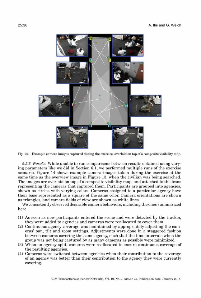
25:36 A. Ilie and G. Welch
Fig. 14. Example camera images captured during the exercise, overlaid on top of a composite visibility map.
6.2.3. Results. While unable to run comparisons between results obtained using vary-ing parameters like we did in Section 6.1, we performed multiple runs of the exercisescenario. Figure 14 shows example camera images taken during the exercise at thesame time as the overview image in Figure 13, when the civilian was being searched.The images are overlaid on top of a composite visibility map, and attached to the iconsrepresenting the cameras that captured them. Participants are grouped into agencies,shown as circles with varying colors. Cameras assigned to a particular agency havetheir base represented as a square of the same color. Camera orientations are shownas triangles, and camera fields of view are shown as white lines.
We consistently observed desirable camera behaviors, including the ones summarizedhere.
(1) As soon as new participants entered the scene and were detected by the tracker,they were added to agencies and cameras were reallocated to cover them.
(2) Continuous agency coverage was maintained by appropriately adjusting the cam-eras’ pan, tilt and zoom settings. Adjustments were done in a staggered fashionbetween cameras covering the same agency, such that the time intervals when thegroup was not being captured by as many cameras as possible were minimized.
(3) When an agency split, cameras were reallocated to ensure continuous coverage ofthe resulting agencies.
(4) Cameras were switched between agencies when their contribution to the coverageof an agency was better than their contribution to the agency they were currentlycovering.
ACM Transactions on Sensor Networks, Vol. 10, No. 2, Article 25, Publication date: January 2014.
Online Control of Active Camera Networks for Computer Vision Tasks 25:37
(5) Continuous ROI coverage was maintained even when ROIs moved quickly or overrelatively large distances by anticipating their trajectory and preemptively adjust-ing the cameras’ pan, tilt and zoom settings.
7. CONCLUSIONS AND FUTURE WORK
We presented a new online camera control approach that treats camera control as anoptimization problem. For the objective function, we developed a versatile performancemetric that can incorporate both performance factors and application requirements. Toreduce the size of the search space and arrive at an implementation that runs in realtime, our camera control method breaks down the optimization problem into subprob-lems. We first employ a proximity-based minimal change heuristic to decompose theproblem into subproblems and a greedy heuristic to assign cameras to subproblemsbased on evaluating candidate plans. We then solve each subproblem independently,generating and evaluating candidate plans as time allows.
We have discussed how our approach can be easily adapted to include require-ments from various computer vision tasks. We demonstrated our approach in simulatedand laboratory experiments, during which we have shown cameras exhibiting behav-iors that facilitate the application of computer vision algorithms to the images theycaptured.
We plan on working on replacing the simulated camera measurements obtained fromthe external tracker with actual measurements from image tracking. We are especiallyinterested in the situation where image tracking is to be performed with the samecameras that are controlled by our approach, which requires the camera control tobalance the requirements of the computer vision application with the requirements ofimage tracking. We are also studying the impact of imprecise geometric calibration andcamera settings precision and accuracy on our control method.
We are working on using knowledge about the environment to correct erroneoustrajectory predictions. For example, if a Kalman filter-based trajectory prediction hasa target passing through a wall, the prediction could be corrected to have the targetstop in front of the wall or walk along it instead.
Our current implementation uses a proximity heuristic for grouping ROIs into agen-cies, and a greedy heuristic for assigning camera agents to agencies. We chose ourheuristics after a careful analysis of the computational complexity of an exhaustivesearch and using our metric to evaluate alternatives, with the overarching goal of re-ducing search space size while still providing a reasonable solution. A thorough analysisof the impact of these heuristics on the solution, as well as a comparison with other ap-proaches, are needed to fully gauge their effectiveness. It would be interesting to exploreother clustering algorithms and evaluate the performance of our method when usingthem. A formal method such as linear programming could be used for assigning camerasto agencies, when feasible, and our heuristic could be run only when such methods fail.A promising direction to explore in clustering would be to allow overlaps, i.e. to allowan ROI to be a member of multiple agencies. Additionally, the current greedy assign-ment scheme exclusively assigns an agent to an agency. There may be situations when,with a small change in its settings, a camera could cover the ROIs in another agencynearby. In such situations, it may be beneficial to explore sharing an agent among mul-tiple agencies. Sharing agents would require a protocol for agencies to cooperate whencomputing the camera parameters for agents that are shared with other agencies.
The main strategy our approach employs to reduce the search space size is decom-posing the problem into subproblems and solving the subproblems at the level of eachagency. Our current implementation solves the subproblems sequentially, in a singlethread. We are working on a parallel implementation that would allow us to evaluatemore candidate plans, increasing the chance that the provided solution is the global
ACM Transactions on Sensor Networks, Vol. 10, No. 2, Article 25, Publication date: January 2014.
25:38 A. Ilie and G. Welch
optimum. Another possible research direction is decentralizing our approach further byhaving “smart” cameras locally estimate their own contribution to each ROI or agency.In the current implementation, the global assignment process is centralized. Distribut-ing the assignment process by making it collaborative is likely to reduce computationloads in large camera networks, possibly at the expense of increased bandwidth re-quired for collaboration, as well as possible additional system latency and weakeroptimal performance guarantees.
REFERENCES
B. D. Allen. 2007. Hardware design optimization for human motion tracking systems. Ph.D. thesis, Universityof North Carolina at Chapel Hill.
B. D. Allen and G. Welch. 2005. A general method for comparing the expected performance of tracking andmotion capture systems. In Proceedings of the 12th ACM Symposium on Virtual Reality Software andTechnology. ACM, 201–210.
A. D. Bagdanov, A. Del Bimbo, and F. Pernici. 2005. Acquisition of high-resolution images through onlinesaccade sequence planning. In Proceedings of the 3rd ACM International Workshop on Video Surveillance& Sensor Networks. 121–130.
A. Bakhtari, M. D. Naish, M. Eskandari, E. A. Croft, and B. Benhabib. 2006. Active-vision-based multisensorsurveillance-an implementation. IEEE Trans. Syst. Man Cybern. Part C Appl. Rev. 36, 5, 668–680.
R. Bodor, P. Schrater, and N. Papanikolopoulos. 2005. Multi-camera positioning to optimize task observability.In Proceedings of the IEEE Conference on Advanced Video and Signal Based Surveillance. 552–557.
C. Broaddus, T. Germano, N. Vandervalk, A. Divakaran, S. Wu, and H. Sawhney. 2009. Activision: Activecollaborative tracking for multiple ptz cameras. In Proceedings of SPIE: Multisensor, Multisource Infor-mation Fusion: Architectures, Algorithms, and Applications. Vol. 7345.
M. Casper. 2007. EventScripts Python. http://python.eventscripts.com.C. B. Chang and J. A. Tabaczyinski. 1984. Application of state estimation to target tracking. IEEE Trans.
Autom. Control 29, 2, 98–109.X. Chen. 2002. Designing multi-camera tracking systems for scalability and efficient resource allocation.
Ph.D. thesis, Stanford University.A. K. R. Chowdhury and R. Chellappa. 2004. An information theoretic criterion for evaluating the quality of
3D reconstructions from video. IEEE Trans. Image Process. 13, 7, 960–973.R. T. Collins, A. J. Lipton, et al. 2000. A system for video surveillance and monitoring. Tech. rep. CMU-RI-
TR-00-12, Robotics Institute, Carnegie Mellon University, Pittsburgh, PA.C. J. Costello, C. P. Diehl, A. Banerjee, and H. Fisher. 2004. Scheduling an active camera to observe people. In
Proceedings of the ACM 2nd International Workshop on Video Surveillance & Sensor Networks. 39–45.J. Davis. 2002. Mixed scale motion recovery. Ph.D. thesis, Stanford University.A. J. Davison and D. W. Murray. 2002. Simultaneous localisation and map-building using active vision. IEEE
Trans. Pattern Anal. Mach. Intell.A. Del Bimbo and F. Pernici. 2005. Towards on-line saccade planning for high-resolution image sensing.
Pattern Recognit. Lett. 27, 15, 1826–1834.J. Denzler and C. Brown. 2002. An information theoretic approach to optimal sensor data selection for state
estimation. IEEE Trans. Pattern Anal. Mach. Intell. 24, 2, 145–157.J. Denzler, C. M. Brown, and H. Niemann. 2001. Optimal camera parameter selection for state estima-
tion with applications in object recognition. In Proceedings of the 23rd DAGM-Symposium on PatternRecognition. Lecture Notes in Computer Science, vol. 2191, 305.
J. Denzler and M. Zobel. 2001. On optimal observation models for kalman filter based tracking approaches.Tech. rep., Lehrstuhl fur Mustererkennung, Universitat Erlangen-Nurnberg.
J. Denzler, M. Zobel, and H. Niemann. 2002. On optimal camera parameter selection in kalman filter basedobject tracking. In Proceedings of the 24th DAGM Symposium on Pattern Recognition. 17–25.
J. Denzler, M. Zobel, and H. Niemann. 2003. Information theoretic focal length selection for real-time ac-tive 3-d object tracking. In Proceedings of the International Conference on Computer Vision. Vol. 1,400–407.
B. Deutsch, H. Niemann, and J. Denzler. 2005. Multi-step active object tracking with entropy based optimalactions using the sequential kalman filter. In Proceedings of the IEEE International Conference on ImageProcessing. Vol. 3, 105–108.
ACM Transactions on Sensor Networks, Vol. 10, No. 2, Article 25, Publication date: January 2014.
Online Control of Active Camera Networks for Computer Vision Tasks 25:39
B. Deutsch, S. Wenhardt, and H. Niemann. 2006. Multi-step multi-camera view planning for real-time visualobject tracking. In Proceedings of the 26th DAGM-Symposium on Pattern Recognition. Lecture Notes inComputer Science, vol. 4174, 536–545.
B. Deutsch, M. Zobel, J. Denzler, and H. Niemann. 2004. Multi-step entropy based sensor control for visualobject tracking. In Proceedings of the 28th DAGM-Symposium on Pattern Recognition. Lecture Notes inComputer Science, vol. 3175, 359–366.
M. S. Grewal and A. P. Andrews. 1993. Kalman Filtering Theory and Practice. Information and SystemSciences Series, Prentice Hall, Upper Saddle River, NJ.
L. Guan. 2010. Multi-view dynamic scene modeling. Ph.D. thesis, University of North Carolina at ChapelHill.
A. Ilie and G. Welch. 2011. On-line control of active camera networks for computer vision tasks. In Proceedingsof the International Conference for Distributed Smart Cameras.
A. Ilie, G. Welch, and M. Macenko. 2008. A stochastic quality metric for optimal control of active cameranetwork configurations for 3D computer vision tasks. In Proceedings of the Workshop on Multi-cameraand Multimodal Sensor Fusion Algorithms and Applications.
D. A. Ilie. 2010. On-line control of active camera networks. Ph.D. thesis, University of North Carolina atChapel Hill.
T. Kailath, A. H. Sayed, and B. Hassibi. 2000. Linear Estimation. Information and System Sciences Series.Prentice Hall, Upper Saddle River, NJ.
N. Krahnstoever, M. Yeasin, and R. Sharma. 2001. Towards a unified framework for tracking and analysis ofhuman motion. In Proceedings of the IEEE Workshop on Detection and Recognition of Events in Video.
N. Krahnstoever, T. Yu, S.-N. Lim, K. Patwardhan, and P. Tu. 2008. Collaborative real-time control of activecameras in large scale surveillance systems. In Proceedings of the Workshop on Multi-Camera andMulti-Modal Sensor Fusion Algorithms and Applications.
S.-N. Lim, A. Mittal, and L. Davis. 2005. Constructing task visibility intervals for a surveillance system. InProceedings of the 3rd ACM International Workshop on Video Surveillance & Sensor Networks. 141–148.
S.-N. Lim, A. Mittal, and L. S. Davis. 2007. Task scheduling in large camera networks. In Proceedings of theAsian Conference on Computer Vision.
L. Marcenaro, F. Oberti, G. L. Foresti, and C. Regazzoni. 2001. Distributed architectures and logical-taskdecomposition in multimedia surveillance systems. Proc. IEEE 89, 10, 1419–1440.
T. Matsuyama and N. Ukita. 2002. Real-time multitarget tracking by a cooperative distributed vision system.Proc. IEEE. 90. 1137–1150.
A. Mittal and L. Davis. 2004. Visibility analysis and sensor planning in dynamic environments. In Proceed-ings of the European Conference on Computer Vision.
A. Mittal and L. S. Davis. 2008. A general method for sensor planning in multi-sensor systems: Extension torandom occlusion. Int. J. Comput. Vision 76, 1, 31–52.
M. D. Naish, E. A. Croft, and B. Benhabib. 2001. Simulation-based sensing-system configuration for dynamicdispatching. In Proceedings of the IEEE International Conference on Systems, Man and Cybernetics.2964–2969.
M. D. Naish, E. A. Croft, and B. Benhabib. 2003. Coordinated dispatching of proximity sensors for thesurveillance of manoeuvring targets. Rob. Comput. Integr. Manuf. 19, 3, 283–299.
P. Natarajan, T. N. Hoang, K. S. Low, and M. Kankanhalli. 2012. Decision-theoretic approach to maximizingobservation of multiple targets in multi-camera surveillance. In Proceedings of the 11th InternationalConference on Autonomous Agents and Multiagent Systems.
F. Oberti, G. Ferrari, and C. S. Regazzoni. 2001. Allocation strategies for distributed video surveillancenetworks. In Proceedings of the International Conference on Image Processing. Vol. 2. 415–418.
G. Olague and R. Mohr. 2002. Optimal camera placement for accurate reconstruction. Pattern Recognit. 35,4, 927–944.
F. Qureshi and D. Terzopoulos. 2007. Surveillance in virtual reality: System design and multi-camera control.In Proceedings of the Conference on Computer Vision and Pattern Recognition. 1–8.
F. Qureshi and D. Terzopoulos. 2005a. Surveillance camera scheduling: a virtual vision approach. In Pro-ceedings of the 3rd ACM International Workshop on Video Surveillance & Sensor Networks. ACM Pres,131–140.
F. Qureshi and D. Terzopoulos. 2005b. Towards intelligent camera networks: A virtual vision approach. InProceedings of the 2nd Joint IEEE International Workshop on Visual Surveillance and PerformanceEvaluation of Tracking and Surveillance. 177–184.
ACM Transactions on Sensor Networks, Vol. 10, No. 2, Article 25, Publication date: January 2014.
25:40 A. Ilie and G. Welch
G. S. Ram, K. Ramakrishnan, P. Atrey, V. K. Singh, and M. S. Kankanhalli. 2006. A design methodology forselection and placement of sensors in multimedia surveillance systems. In Proceedings of the 4th ACMInternational Workshop on Video Surveillance & Sensor Networks.
P. Remagnino, A. Shihab, and G. Jones. 2003. Distributed intelligence for multi-camera visual surveillance.Pattern Recognit. 37, 4, 675–689.
E. Sommerlade and I. Reid. 2008a. Cooperative surveillance of multiple targets using mutual informa-tion. In Proceedings of the Workshop on Multi-camera and Multi-modal Sensor Fusion Algorithms andApplications.
E. Sommerlade and I. Reid. 2008b. Information theoretic active scene exploration. In Proceedings of theIEEE Conference on Computer Vision and Pattern Recognition.
E. Sommerlade and I. Reid. 2008c. Information-theoretic decision making for exploration of dynamic scenes.In Proceedings of the 5th International Workshop on Attention in Cognitive Systems.
E. Sommerlade and I. Reid. 2010. Probabilistic surveillance with multiple active cameras. In Proceedings ofthe IEEE International Conference on Robotics and Automation.
P.-N. Tan, M. Steinbach, and V. Kumar. 2005. Introduction to Data Mining. Addison-Wesley.K. A. Tarabanis, R. Y. Tsai, and P. K. Allen. 1995. A survev of sensor planning in computer vision. IEEE
Trans. Rob. Autom. 11, 1, 86–104.G. R. Taylor, A. J. Chosak, and P. C. Brewer. 2007. OVVV: Using virtual worlds to design and evaluate surveil-
lance systems. In Proceedings of the IEEE Conference on Computer Vision and Pattern Recognition. 1–8.G. Welch, B. D. Allen, A. Ilie, and G. Bishop. 2007. Measurement sample time optimization for human motion
tracking/capture systems. In Proceedings of the Workshop on Trends and Issues in Tracking for VirtualEnvironments at the IEEE Virtual Reality Conference. G. Zachmann, Ed.
G. Welch and G. Bishop. 2001. An introduction to the Kalman filter: SIGGRAPH 2001 course 8. In ComputerGraphics SIGGRAPH 2001 Course Pack. ACM Press, Addison-Wesley Publishing Company, Los Angeles,CA.
J. J. Wu, R. Sharma, and T. S. Huang. 1998. Analysis of uncertainty bounds due to quantization for three-dimensional position estimation using multiple cameras. Opt. Eng. 37, 280–292.
S. Yous, N. Ukita, and M. Kidode. 2007. An assignment scheme to control multiple pan/tilt cameras for 3dvideo. J. Multimedia 2, 1, 10–19.
Z. Zhang. 1999. Flexible camera calibration by viewing a plane from unknown orientations. In Proceedingsof the International Conference on Computer Vision.
Received March 2012; revised October 2012; accepted January 2013
ACM Transactions on Sensor Networks, Vol. 10, No. 2, Article 25, Publication date: January 2014.