Online Balanced Repartitioning of Dynamic Communication ...

Online Balanced Repartitioning ofDynamic Communication Patterns in Polynomial Time∗

Tobias Forner† Harald Racke‡ Stefan Schmid§

Abstract

This paper revisits the online balanced repartitioning prob-

lem (introduced by Avin et al. at DISC 2016) which asks for

a scheduler that dynamically collocates frequently communi-

cating nodes, in order to reduce communication costs while

minimizing migrations in distributed systems. More specif-

ically, communication requests arrive online and need to be

served, either remotely across different servers at cost 1, or

locally within a server at cost 0; before serving a request, the

online scheduler can change the mapping of nodes to servers,

i.e., migrate nodes, at cost α per node move. Avin et al.

presented a deterministic O(k log k)-competitive algorithm,

Crep, which is optimal up to a logarithmic factor; however,

their algorithm has the drawback that it relies on expensive

repartitioning operations which result in a super-polynomial

runtime. Our main contribution is a different deterministic

algorithm pCrep which achieves the same competitive ra-

tio, but runs in polynomial time. Our algorithm monitors

the connectivity of communication requests over time, rather

than the density as in prior work by Avin et al.; this enables

the polynomial runtime. We analyze pCrep both analyti-

cally and empirically.

1 Introduction

Most distributed systems critically rely on an efficientinterconnecting communication network. With the in-creasing scale of these systems, the network trafficoften grows accordingly: applications related to dis-tributed machine learning, batch processing, or scale-out databases, spend a considerable fraction of theirruntime shuffling data [1]. An interesting approach toimprove the efficiency in these systems is to exploit theirresource allocation flexibilities: many distributed sys-tems are highly virtualized today and support to relo-cate (or migrate) communication partners (e.g. virtualmachines). By collocating two frequently communicat-

∗Supported by European Research Council (ERC) Consolida-

tor project, Self-Adjusting Networks (AdjustNet), grant agree-ment No. 864228, Horizon 2020, 2020-2025.

†Technical University Munich, Germany.‡Technical University Munich, Germany.§Faculty of Computer Science, University of Vienna, Austria.

ing nodes on the same server, slow and costly inter-server communication can be reduced. However, reloca-tions also come at a cost, and the number of migrationsshould be kept low.

This paper revisits the online balanced repartition-ing problem [2] which models the tradeoff between thebenefits and the costs of dynamic relocations. The goalis to design an algorithm which maintains, at any time,a mapping of n communication nodes (virtual machines)to ` servers of fixed equal size k; in the absence of aug-mentation, n = `k. The communication pattern can beseen as a dynamic graph, from which communicationrequests arrive in an online manner; in other words,the online algorithm does not have prior knowledge offuture communication requests. The goal is to strikea balance between the benefits and the costs of migra-tions. More specifically, the cost model is as follows: if acommunication request is served remotely, i.e., betweennodes mapped to different servers, it incurs a communi-cation cost of 1; communication requests between nodeslocated on the same server are free of cost. Before thecost for the current request is paid, an algorithm hasthe option to migrate nodes at a cost of α > 1 for eachnode move.

The problem can be seen as a symmetric version ofcaching: two nodes can be “cached” together on anyserver.

1.1 Contributions Our main result is a determinis-tic online algorithm pCrep for the dynamic balancedgraph partitioning problem which achieves a competi-tive ratio of O(k log k) and runs in polynomial time, fora constant augmentation.

A O(k log k)-competitive algorithm, Crep, was al-ready given by Avin et al. in [2], together with an almosttight lower bound Ω(k). However, the algorithm relieson expensive repartitioning which results in a super-polynomial runtime. Our algorithm, pCrep, is similarto the algorithm by Avin et al., but it comes with atwist: rather than considering the density of emergingcommunication patterns when deciding the repartition-ing, we consider the connectivity. The latter allows forpolynomial-time approximations, as we will show, but

Copyright © 2021 by SIAMUnauthorized reproduction of this article is prohibited

also requires a new analysis.Besides the analytical evaluation, we report on

simulations based on real datacenter workloads. Ourimplementation is publicly available as open source [3].

1.2 Preliminaries Let us introduce some definitionsand notations that will be used throughout the paper.We define a graph G = (V,E,w) where V is theset of vertices, E the set of (undirected) edges, andw : E → N assigns each edge an (integer) weight.Given a graph G = (V,E,w), we define an (edge) cutof G as a pair of two disjoint subsets X,Y of V suchthat X ∪ Y = V . The value of this cut is the sum ofthe weight of edges between nodes from X and Y , i.e.∑e=u,v∈E:u∈X,v∈Y w(e) is the value of the cut (X,Y ).

Note that such a cut can also be defined by the set ofthe edges connecting X and Y that are cut. We call acut a minimum (edge) cut of G if it is one of the cutswith minimum value.

The connectivity of a graph G is equal to the valueof a minimum edge cut of G. This definition will beused in order to define the communication componentsour algorithm maintains as these are subsets of V whichinduce subgraphs of high connectivity. We explain theconcept of components in greater detail later.

Furthermore we define the term (s, t)-cut as a cut(X,Y ) for which s ∈ X and Y ∈ X, i.e. a (s, t)-cutseparates the nodes s and t in G. Then a minimum(s, t)-cut is a (s, t)-cut of minimum value. Note that aminimum (s, t)-cut is not necessarily a minimum cut.

Finally we sometimes call a function m : X → Ya mapping of X to Y . We use this terminology forexample when we talk about the assignment of nodes toservers.

2 Model

We consider the problem of maintaining a partitioningof a set of n = k · ` nodes (e.g., processes or virtualmachines) that communicate with each other, into `servers (henceforth sometimes also called clusters) ofsize k each, while minimizing both the cost due tocommunication and due to node migrations. Moreformally we are given ` servers V0, ..., V`−1, each withcapacity k and an initial perfect mapping of n =k · ` nodes to the ` servers, i.e. a mapping in whicheach server is assigned exactly k nodes. An inputsequence σ = ((u1, v1), 1), ((u2, v2), 2), ...((ui, vi), i), ...describes the sequence of communication requests: thepair ((ut, vt), t) represents a communication requestbetween the nodes ut and vt arriving at time t. At timet the algorithm is allowed to perform node migrationsat a cost of α > 1 per move. After the migration step,the algorithm pays cost 1 if ut and vt are mapped to

different servers and does not pay any cost otherwise.Note that an algorithm may also choose to perform nomigrations at all.

We are in the realm of competitive analysis andas a result we compare an online algorithm ONL tothe optimal offline algorithm OPT. ONL only learns ofthe requests in the input sequence σ as they happenand as a result only knows about the partial sequence(u1, v1), ..., (ut, vt) at time t whereas OPT has perfectknowledge of the complete sequence σ at all times.

The goal is to design an online algorithm ONL witha good competitive ratio with regard to OPT definedas follows. An online algorithm ONL is ρ-competitive ifthere exists a constant β such that

ONL(σ) ≤ ρ ·OPT(σ) + β ∀σ

where ONL(σ) and OPT(σ) denote the cost of servinginput sequence σ of ONL and OPT respectively. Thishas to hold for any input sequence σ.

We consider a model with augmentation (as in priorwork [2]), and allow the online algorithm to use largercapacities per server. In particular, the online algorithmis allowed to assign (2 + ε) · n/` nodes to each serverwhere ε > 0. This augmented online algorithm is thencompared with the optimal offline algorithm OPT whichis not allowed to use any augmentation.

Throughout this paper, we will also use 1 + ε as thebasis for the logarithm.

3 Basic Algorithm

We first describe the basic algorithm underlying our ap-proach, before presenting the polynomial-time imple-mentation later in this paper. In general, pCrep re-lies on a second-order partitioning of the communicationnodes into communication components which representnode-induced sub-graphs of the original communicationgraph given by the requests from the input sequenceσ. To this end we define a component C as the setof its nodes together with the time t of its creation, i.e.C = (v1, v2, ..., vk, t). For a component B = (M, t) letnodes(B) = M , τ(B) = t and we define |B| = |M | inorder to improve readability. Initially each node formsa singleton component, but as the input sequence σ isrevealed, new communication patterns unfold. The al-gorithm keeps track of these patterns by maintaining agraph in which the nodes represent the actual communi-cation nodes and the weighted edges represent the num-ber of communication requests between nodes that werepart of different components at the time of the request;that is, for edge e = u, v, w(e) represents the numberof paid communication requests between u and v. Wesay that a communication request between nodes u andv is paid if the nodes are located on different servers


at the time of the request. The algorithm merges a setS of components, which we will refer to as a compo-nent set, into a new component C if the connectivityof the component graph induced by the components inS is at least α. After each edge insertion the algorithmchecks whether there exists a new component set S with|S| > 1 which fulfills this requirement.

If after any request and the insertion of the resultingedge the algorithm discovers a new subset S of nodeswhose induced subgraph has connectivity at least αand which is of cardinality at most k, it merges thecomponents that form this set into one new componentand collocates all the nodes in the resulting set on asingle server. The algorithm reserves additional spacemink − |C|, bε · |C|c for each component of size |C|on the server it is currently located on. Note thatthe additional reservation may be zero for componentssmaller than 1/ε. This reservation guarantees thatnodes are not migrated too often for the analysis towork. This also limits the total space a componentcan use to a maximum of k. This makes sense as acomponent whose size exceeds k is split (rather thanmerged). To this end the algorithms keep track of thereservations for each component.

The algorithm uses augmentation 2 + ε in orderto guarantee that the collocation of such componentsets of at most k individual communication nodes isalways possible without moving a node not in C. Thisguarantees by an averaging argument that there isalways at least one cluster with capacity at least k,which a newly merged component can be moved to.

If the subset has cardinality greater than k, thecomponents that form this set are split. We also givea pseudocode description of the algorithm in which wedenote the reservation of a component C by res(C) andthe current server it is mapped to by serv(C). Thefree capacity of a server i is denoted by cap(i). Thegeneral structure of our algorithm is summarized inAlgorithm 1. In the case of a merge the subroutineAlgorithm 2 is called which first increases the capacitiesof the involved servers by the reserved amounts of thecomponents that are to be merged. In a second stepthe subroutine Algorithm 4 moves the nodes to a serverof suitable capacity and claims the space required forthe nodes as well as additional reservations. In the caseof a split subroutine Algorithm 3 is called which splitsthe components and frees up the additional reservations.The capacity used for the nodes involved is not changed.

The main differentiating factor of this approachcompared to prior work [2, 4] is that we merge oncea component set reaches connectivity α, while priorapproaches do so once the component set reaches acertain density threshold. More specifically earlier

Algorithm 1 pCrep

G ← (1, ..., n, ∅, w) //initialize a graph on n nodeswithout edges, w assigns 0 to every edgeturn each of the n nodes into a singleton componentfor all r = ((u, v), t) ∈ σ do

if comp(v) 6= comp(u) thenw(u, v)← w(u, v) + 1

end ifif ∃ component set X with connectivity at least αand |X| > 1 and nodes(X) ≤ k then

mergeAndRes(X)end ifif ∃ component set Y with connectivity at least αand nodes(Y ) > k then

split(Y ) // to be specified laterend if

end for

Algorithm 2 mergeAndRes(X)

for all C ∈ X docap(serv(C))← cap(serv(C)) + res(C)

end forcollocate(X) // moves all components from X to thesame server as described

algorithms merge a component set S once it fulfillsw(S) ≥ (|S| − 1) ·α where w(S) denotes the cumulativeweight of the edges between nodes contained in thecomponents of S.

Algorithm 3 split(Y ) of pCrep

for all e = u, v ∈ E doif u ∈ Y or v ∈ Y thenw(e)← 0

end ifend forfor all C ∈ Y docap(serv(C))← cap(serv(C)) + res(C)res(C)← 0

end for

pCrep resets all the edges contained in the splitcomponent C and also resets the weights of edgesadjacent to C, i.e. all edges e = u, v are reset to zeroif u or v were contained in component C at the timeof its split. The splitting method is also described inpseudocode in Algorithm 3. Additionally, Algorithm 4describes the collocation procedure that first tries tofind a component such that the remaining ones that areto be merged fit into its existing reservation (if-case). Ifthis is not possible all the components that are to be


Algorithm 4 collocate(X)

Cmerged ←⋃C∈X C

if ∃C ∈ X s.t. res(C) >= |Cmerged| − |C| thenmove all nodes from Cmerged to the server of C,freeing reservations and capacityres(Cmerged)← res(C)− (|Cmerged| − |C|)

elsetarget ← server s.t. cap(server) ≥ mink, b(1 +ε) · |Cmerged|cmove all nodes from Cmerged to target, freeingreservations and capacitycap(target) ← cap(target) − mink, b(1 + ε) ·|Cmerged|cres(Cmerged)← mink − |Cmerged|, bε · |Cmerged|c

end if

merged are moved to a new server with enough spacefor the resulting merged component Cmerged as wellas the additional reservation of mink − |Cmerged|, bε ·|Cmerged|c. Furthermore the merge and split processis illustrated in Figure 1.

As we will see, the idea for the competitive analysisis to relate the cost of both OPT and pCrep to thesplit components in the solution of pCrep. The factthat pCrep also resets adjacent edges means that wecan uniquely identify requests with the split componentwhose split led to the reset of the corresponding edgeweights to zero.

4 Competitive Analysis

We analyze the competitive ratio of pCrep with aug-mentation (2+ε) and show that pCrep isO(2/ε·k log k)-competitive. We will use the following general defini-tions throughout the analysis.

Definition 4.1. For any subset S of components, letw(S) be the total weight of all edges between nodes of S.

Definition 4.2. We call a set of components of size atleast 2 and of connectivity α mergeable.

Definition 4.3. An α-connected component is a max-imal set of vertices that is α-connected.

Despite the algorithmic differences, some claimsfrom [4] can be adapted for pCrep. In particular, wecan show that there is always at most one mergeablecomponent set after the insertion of a new edge whichpCrep then merges. The earliest point in time a newmergeable component set can emerge is after the nextedge is inserted. In the following, we will now focus onthe novel aspects of the competitive analysis.

0 5 10 15 20

1

2

3

4

5

6

7

time

nod

es

Figure 1: Illustration for the pCrep approach: Thehorizontal lines represent the nodes over time, verticallines represent requests between the respective endpoints. We consider the case where α = 3 and k =3. At time t = 3 the nodes 1 and 2 are merged,resulting in component C1 = (1, 2, 3). The next threerequests lead pCrep to merge the singleton component(3, 0) with C1, resulting in the component C2 =(1, 2, 3, 6). The following eight requests connect thesingleton components containing the nodes 4, 5, 6 and7 to C2, but the respective cuts have value 2, henceno merge is performed. At time t = 15 finally theedge weight between the component of node 4 and C2

increases to 3. Now the subgraph induced by the setof nodes M = 1, 2, 3, 4 has connectivity 3, but as|M | = 4 > 3 = k pCrep splits the components. Duringthis split all edge weights representing the requestsshown in the figure are reset to zero, both those thatled to the merges and the remaining ones.


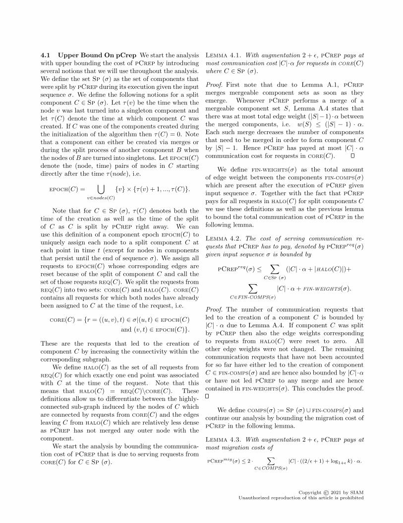
4.1 Upper Bound On pCrep We start the analysiswith upper bounding the cost of pCrep by introducingseveral notions that we will use throughout the analysis.We define the set Sp (σ) as the set of components thatwere split by pCrep during its execution given the inputsequence σ. We define the following notions for a splitcomponent C ∈ Sp (σ). Let τ(v) be the time when thenode v was last turned into a singleton component andlet τ(C) denote the time at which component C wascreated. If C was one of the components created duringthe initialization of the algorithm then τ(C) = 0. Notethat a component can either be created via merges orduring the split process of another component B whenthe nodes of B are turned into singletons. Let EPOCH(C)denote the (node, time) pairs of nodes in C startingdirectly after the time τ(node), i.e.

EPOCH(C) =⋃

v∈nodes(C)

v × τ(v) + 1, ..., τ(C).

Note that for C ∈ Sp (σ), τ(C) denotes both thetime of the creation as well as the time of the splitof C as C is split by pCrep right away. We canuse this definition of a component epoch EPOCH(C) touniquely assign each node to a split component C ateach point in time t (except for nodes in componentsthat persist until the end of sequence σ). We assign allrequests to EPOCH(C) whose corresponding edges arereset because of the split of component C and call theset of those requests REQ(C). We split the requests fromREQ(C) into two sets: CORE(C) and HALO(C). CORE(C)contains all requests for which both nodes have alreadybeen assigned to C at the time of the request, i.e.

CORE(C) = r = ((u, v), t) ∈ σ|(u, t) ∈ EPOCH(C)

and (v, t) ∈ EPOCH(C).

These are the requests that led to the creation ofcomponent C by increasing the connectivity within thecorresponding subgraph.

We define HALO(C) as the set of all requests fromREQ(C) for which exactly one end point was associatedwith C at the time of the request. Note that thismeans that HALO(C) = REQ(C)\CORE(C). Thesedefinitions allow us to differentiate between the highly-connected sub-graph induced by the nodes of C whichare connected by requests from CORE(C) and the edgesleaving C from HALO(C) which are relatively less denseas pCrep has not merged any outer node with thecomponent.

We start the analysis by bounding the communica-tion cost of pCrep that is due to serving requests fromCORE(C) for C ∈ Sp (σ).

Lemma 4.1. With augmentation 2 + ε, pCrep pays atmost communication cost |C|·α for requests in CORE(C)where C ∈ Sp (σ).

Proof. First note that due to Lemma A.1, pCrepmerges mergeable component sets as soon as theyemerge. Whenever pCrep performs a merge of amergeable component set S, Lemma A.4 states thatthere was at most total edge weight (|S|−1) ·α betweenthe merged components, i.e. w(S) ≤ (|S| − 1) · α.Each such merge decreases the number of componentsthat need to be merged in order to form component Cby |S| − 1. Hence pCrep has payed at most |C| · αcommunication cost for requests in CORE(C).

We define FIN-WEIGHTS(σ) as the total amountof edge weight between the components FIN-COMPS(σ)which are present after the execution of pCrep giveninput sequence σ. Together with the fact that pCreppays for all requests in HALO(C) for split components Cwe use these definitions as well as the previous lemmato bound the total communication cost of pCrep in thefollowing lemma.

Lemma 4.2. The cost of serving communication re-quests that pCrep has to pay, denoted by pCrepreq(σ)given input sequence σ is bounded by

pCrepreq(σ) ≤∑

C∈Sp (σ)

(|C| · α+ |HALO(C)|)+

∑C∈FIN-COMPS(σ)

|C| · α+ FIN-WEIGHTS(σ).

Proof. The number of communication requests thatled to the creation of a component C is bounded by|C| · α due to Lemma A.4. If component C was splitby pCrep then also the edge weights correspondingto requests from HALO(C) were reset to zero. Allother edge weights were not changed. The remainingcommunication requests that have not been accountedfor so far have either led to the creation of componentC ∈ FIN-COMPS(σ) and are hence also bounded by |C| ·αor have not led pCrep to any merge and are hencecontained in FIN-WEIGHTS(σ). This concludes the proof.

We define COMPS(σ) := Sp (σ) ∪ FIN-COMPS(σ) andcontinue our analysis by bounding the migration cost ofpCrep in the following lemma.

Lemma 4.3. With augmentation 2 + ε, pCrep pays atmost migration costs of

pCrepmig(σ) ≤ 2 ·∑

C∈COMPS(σ)

|C| · ((2/ε+ 1) + log1+ε k) · α.


Proof. Consider the cases in Algorithm 4 in whichcomponents are migrated after a merge. In the if-case only components are moved that fit into thereservation of some merged component C with enoughfree reservation, hence the number of migrated nodesis at most ε · |C| ≤ |C|. Hence only components aremoved whose size is at most half the size of the resultingcomponent Cmerged. Hence each node is merged at mostlog2 k times during the time it is in EPOCH(B) for someB ∈ Sp (σ).

In the else-case components are moved if none ofthe reservations of the merged components in X areenough to fit Cmerged. Again we observe that this mayonly happen at most log1+ε k times, hence each node vof some split component B ∈ Sp (σ) that contains v ismoved at most log1+ε k times during the time it is inEPOCH(B).

In addition components may be moved if the com-ponents are still small and thus their reservations arerounded to zero. This may only lead to at most 2/εmigrations per node in B ∈ Sp (σ).

Hence we may bound the migration cost of pCrepby summing over components in Sp (σ)∪FIN-COMPS(σ):

pCrepmig(σ) ≤∑

C∈COMPS(σ)

(|C| · ((2/ε) + log2 k)

+ |C| · ((2/ε) + log1+ε k)) · α

≤ 2 ·∑

C∈COMPS(σ)

|C| · ((2/ε) + log1+ε k) · α.

We combine our results from Lemma 4.2 andLemma 4.3 in the following lemma in order to obtainthe final upper bound on the cost of pCrep.

Lemma 4.4. With augmentation 2 + ε, pCrep pays atmost total cost

3 ·∑

C∈COMPS(σ)

|C| · ((2/ε+ 1) + log1+ε k) · α

+∑

C∈Sp (σ)

|HALO(C)|+ FIN-WEIGHTS(σ).

where COMPS(σ) = Sp (σ) ∪ FIN-COMPS(σ).

Proof. We use the results from Lemma 4.2 and

Lemma 4.3 to obtain the lemma:

pCrep(σ) ≤ pCrepreq(σ) + pCrepmig(σ)

≤∑

C∈Sp (σ)

(|C| · α+ |HALO(C)|)

+∑

C∈FIN-COMPS(σ)

|C| · α+ FIN-WEIGHTS(σ)

+ 2 ·∑

C∈COMPS(σ)

|C| · ((2/ε+ 1) + log1+ε k) · α

≤ 3 ·∑

C∈COMPS(σ)

|C| · ((2/ε+ 1) + log1+ε k) · α

+∑

C∈Sp (σ)

|HALO(C)|+ FIN-WEIGHTS(σ).

4.2 Lower Bound on OPT We next bound the coston OPT by assigning cost to OPT based on the size ofthe components C that pCrep resets and the associatedadjacent edges HALO(C) which pCrep resets to zeroduring the split of C. In order to achieve this weintroduce some additional notions. First we define theterm offline interval of a node v to be the time betweentwo migrations of v in the solution of OPT. Morespecifically let T (v) = (t0, t1, t2, ...) denote the orderedsequence of the times at which OPT migrates node vwith the addition of t0 = 0 such that for all i, ti < ti+1 ifti, ti+1 ∈ T (v). Then an offline interval (ti, ti+1] of nodev is defined by every two subsequent times in T (v).

Furthermore we say that an offline interval (ti, ti+1]of node v ∈ C is contained in the epoch EPOCH(C) of acomponent C ∈ Sp (σ) if it ends before the time τ(C),i.e. if ti+1 < τ(C). Note that τ(C) is both the timeof the creation of C in the solution of pCrep and thetime of its split as C ∈ Sp (σ). We assign a request roccurring at time τ(r) that involves the nodes v and uto an offline interval I = (ti, ti+1] of v if τ(r) ∈ I and ifit is both the first offline interval of one of the end pointsof r that ends and if the offline interval ends before thedeletion of the edge representing r due to a componentsplit, i.e. let t be the time of the component splitthat resets the edge corresponding to r and (tj , tj+1])be the offline interval of node u that contains τ(r),then ti+1 < t and ti+1 < tj+1. The requests fromH =

⋃C∈Sp (σ) HALO(C) that are not assigned to any

offline interval are then those which are reset due tothe split of a component that took place before thecorresponding offline interval ended. Let P denote theset of edges from

⋃C∈Sp (σ) HALO(C) that both pCrep

and OPT pay for and let I denote the set of requests wehave assigned to offline intervals.

These definitions are illustrated in Figure 2. Note


1

2

3

4

5

6

7

nodes

time

EPOCH(C) outline

OPT migration

split of component

Figure 2: Illustration of definitions used in the analy-sis; vertical lines represent requests between the corre-sponding nodes; dashed black requests are assigned toanother component; the dashed green line is assigned tothe offline interval of node 5; the regular green lines areassigned to an offline interval which is not contained inEPOCH(C).

that we only show some requests explicitly for the sakeof readability. The grey horizontal lines represent thenodes at each time t. The brown outline surroundsthe (node,time) pairs of EPOCH(C). Blue dots markmigrations of the corresponding node performed by OPT

while brown dots mark splits of the component the nodewas assigned to at that time. The dashed vertical linesin black mark requests that are assigned to anothercomponent because it is split before component C. Thedashed green line is a request from HALO(C) assigned tothe offline interval of node 5 between the two blue dots.The regular green lines are assigned to an offline intervalwhich is not contained in EPOCH(C). We define thisconcept more formally at a later point in the analysis.The lines in magenta are sample requests from CORE(C).

We start by bounding the total edge weight (thetotal number of requests) we assign to any one offlineinterval when limiting ourselves to requests from Hwhich pCrep pays for but OPT does not. We denotethe set of these requests by N , i.e. N = H\P . Notethat H only contains requests which pCrep payed fordue to the definition of HALO(C).

Lemma 4.5. We assign at most k · α requests from Nto any one offline interval.

Proof. We fix an arbitrary offline interval of node v.

Observe that none of the nodes involved in the assignedrequests are moved by OPT during the offline interval,hence all the requests in question involve only nodesthat OPT has placed on the same server as v during theoffline interval.

The number of such nodes is hence limited by theserver capacity k. As we only examine requests from Hwe know that none of these requests have led pCrepto perform any merges, hence there were at most αrequests between v and any one of the other nodes onits server during the offline interval. This bounds thenumber of requests assigned to the offline interval byk · α.

Let R(C) denote the set of requests fromHALO(C)\P that were not assigned to any offline in-terval for a split component C ∈ Sp (σ) and that OPT

does not pay for. We say that a migration of node v attime t in the solution of OPT is contained in EPOCH(C)if (v, t) ∈ EPOCH(C). Let OPT-MIG(C) denote the costof OPT due to migrations of nodes from component Cthat are contained in EPOCH(C) and let OPT-REQ(C)denote the cost of OPT due to serving requests fromCORE(C). We show the following lower bound on thecost of OPT for migrations from OPT-MIG(C) and re-quests from OPT-REQ(C) for all split components C.

Lemma 4.6.∑C∈Sp (σ)

OPT-MIG(C) + OPT-REQ(C) ≥

1/2 ·∑

C∈Sp (σ)

|C|/k · α+ |R(C)|/k

Proof. For the following part of the proof we fix anarbitrary component C ∈ Sp (σ). Note that the nodesinvolved in requests from R(C) were not moved byOPT during the processing of requests from R(C) untilthe time of the split of C as otherwise they would beassigned to an offline interval.

The number of nodes contained in C or connectedto C via edges representing requests from R(C) is atleast |C| + |R(C)|/α since requests from R(C) havenot led pCrep to perform any migrations. Becauseof this fact OPT must have placed those nodes on at

least |C|+|R(C)|/αk different servers. As OPT does not

pay for any requests from R it follows that OPT musthave placed the nodes from C in (|C| + |R(C)|/α)/kdifferent servers.

We first examine the case in which OPT does notmove any nodes from C during EPOCH(C). In this caseOPT must partition a graph containing the nodes from Cwhich are connected via edges representing the requestsfrom CORE(C). As stated earlier OPT placed those


nodes in (|C| + |R(C)|/α)/k different servers at timeτ(C). As pCrep merged component C this graph is α-connected and hence Lemma A.3 gives that OPT has tocut at least edges of total weight ((|C|+|R(C)|/α)/k)/2·α = 1/2 · (|C|/k · α+ |R(C)|/k).

For the more general case in which OPT mayperform node migrations during EPOCH(C) we adaptthe graph construction from above as follows: weadd a vertex representing each (node, time) pair fromEPOCH(C). We connect each (node, time) pair p withedges of weight α to the pairs of the same node thatrepresent the time step directly before and directly afterp (if they exist in the graph). These edges represent thefact that OPT may choose to migrate a node betweenany two time steps in EPOCH(C). Additionally we addan edge of weight one for each request r = ((u, v), t)from CORE(C) by connecting the nodes in the graph thatrepresent the pairs (u, t) and (v, t), respectively. OPT

once again has to partition this graph into |C|+|R(C)|/αk

parts. Note that we only added edges of weight α tothe graph and hence this graph is also α-connected. Weconclude that once again OPT has to cut edges of weight

at least |C|+|R(C)|/αk ·1/2·α = 1/2·(|C|/k ·α+|R(C)|/k).

In both cases only edges representing either requestsfrom OPT-REQ(C) or migrations from OPT-MIG(C) werecut. As the sets CORE(C), R(C) , CORE(D) and R(D)are disjoint for two different components C,D ∈ Sp (σ)per their definition we conclude that∑

C∈Sp (σ)

OPT-MIG(C) + OPT-REQ(C) ≥

1/2 ·∑

C∈Sp (σ)

|C|/k · α+ |R(C)|/k.

In the following lemma we combine the results ofthe previous lemmas in order to bound the cost of OPT

given input sequence σ, denoted by OPT(σ).

Lemma 4.7. The cost of the solution of OPT giveninput sequence σ is bounded by

OPT(σ) ≥ 1/4 ·∑

C∈Sp (σ)

|C|/k · α+ |HALO(C)|/k.

Proof. We combine the results from Lemma 4.5 andLemma 4.6. Note that the cost from Lemma 4.6 maycontain migration costs. In this case the correspondingmigrations represent the end of an offline interval. Wedenote the number of offline intervals by o. This givesus that

2OPT(σ) ≥∑

C∈Sp (σ)

OPT-MIG(C) + OPT-REQ(C) + o · α+ |P |

as we account for each migration at most twice.Consider that due to Lemma 4.5 we have the

inequality o ≥ |N |/k. We repeat that H =⋃C∈Sp (σ) HALO(C). Note that N is the subset of re-

quests of H for which OPT does not pay while P is thesubset of H OPT pays for. It follows that the disjointunion of N and P is H. Hence we obtain

2OPT(σ) ≥∑

C∈Sp (σ)

OPT-MIG(C) + OPT-REQ(C) + o · α+ |P |

≥∑

C∈Sp (σ)

1/2 · (|C|/k · α+ |R(C)|/k) + (|N |+ |P |)/k

≥ 1/2 ·∑

C∈Sp (σ)

|C|/k · α+ |HALO(C)|/k.

This completes the proof.

4.3 Competitive Ratio We can now combine theresults of Lemma 4.4 and Lemma 4.7 to obtain the fol-lowing theorem which gives us the desired competitiveratio.

Theorem 4.1. With augmentation (2 + ε) the compet-itive ratio of pCrep is in O(2/ε · k log1+ε k).

Proof. We arbitrarily fix an input sequence σ and useour previous results to bound the competitive ratio ofpCrep. We define COMPS(σ) := Sp (σ)∪ FIN-COMPS(σ)and c := 2/ε+ 1 in order to improve readability.

pCrep(σ)− FIN-WEIGHTS(σ)

OPT(σ)

≤3 ·

∑C∈COMPS(σ) |C| · (c+ log1+ε k) · α+

∑C∈Sp (σ) |HALO(C)|

1/4 ·∑C∈Sp (σ) |C|/k · α+ |HALO(C)|/k

≤ k log1+ε k3 ·

∑C∈Sp (σ) |C| · c · α+

∑C∈Sp (σ) |HALO(C)|

1/4∑C∈Sp (σ)(|C| · α/2 + |HALO(C)|)

+ β

= O(2/ε · k log1+ε k) + β

where

β =∑

C∈FIN-COMPS(σ)

|C| · ((2/ε+ 1) + log1+ε k) · α

Let β′ = β + FIN-WEIGHTS(σ). Then it follows that

pCrep(σ)

OPT(σ)≤ O(2/ε · k log1+ε k) + β′.

To obtain the bound on β′ we observe that thecomponents in FIN-COMPS(σ) each are of size at mostk since they were not split by pCrep. This allowsus to derive the bound

∑C∈FIN-COMPS(σ) |C| · ((2/ε +

1) + log1+ε k) ≤ ` · k · ((2/ε + 1) + log1+ε k). Since


at the end of the execution of pCrep there can be atmost k · ` components, Lemma A.4 allows us to boundFIN-WEIGHTS(σ) by k ·` ·α. Hence we conclude that β′ ≤`·k ·((2/ε+1)+log1+ε k)·α+k ·`·α ∈ O(2/ε·k log1+ε k).

5 Poly-Time Implementation

So far we have only shown that the Algorithm pCrepdescribed in Section 3 has a competitive ratio O(2/ε ·k log1+ε k). We now show that it can also be imple-mented in polynomial time.

In order to limit the section of the graph G main-tained by pCrep that needs to be updated upon anew request between nodes of different components, wemaintain a decomposition tree defined as follows: theroot represents the whole graph and is assigned the con-nectivity of the entire graph. Given a node v in thetree that represents a subgraph G′ of G, we decomposeG′ into subgraphs whose connectivity is strictly largerthan that of G′ and add children to v for each suchsubgraph. We do not decompose sub-graphs of connec-tivity at least α any further as we only need to identifywhether a new subgraph of connectivity at least α wascreated by the insertion of the most recent request. Ad-ditionally we keep track of the connectivity of each suchsubgraph. In the decomposition tree we have labelledeach node with the corresponding subset of vertices andthe connectivity of the graph induced by these vertices.

If a new request is revealed to pCrep then we onlyneed to update the smallest subtree of the decompo-sition tree which still contains both end points of therequest. This is correct because we can view each de-composition of a subgraph G′ into smaller graphs of ahigher connectivity as a set of cuts that separates thenodes of G′. Inserting a new edge within a subgraphG′ may only increase the value of the cuts which re-sult in the decomposition of G′, but does not affect cutsseparating G′ itself from other subgraphs. If a new re-quest led to the creation of a new component this meansthat two old components that were at least α-connectedwere merged and hence the number of leaves in the de-composition tree decreased. If this is the case then thealgorithm checks whether the new component containsmore than k nodes. In this case the component is splitand split into singleton components, each containing onenode from the split component.

Upon such a component split the edges inside of andadjacent to the component are deleted, i.e. their weightis reset to zero. This means that the decompositiontree needs to be recomputed in order to reflect thischange. If however the resulting component C containsat most k nodes the algorithm tries to collocate thenodes of the component while minimizing migration

costs, i.e. looking for a cluster which contains as manynodes of the newly merged component as possible butwhich also has enough free capacity for the remainingnodes to be moved there and for additional reservationmink − |C|, bε · |C|c.

5.1 Subgraph Decomposition We next describeour algorithm for the decomposition of a given subgraphrepresented by a node in the decomposition tree.

Given a node v of the decomposition tree, first apartition graph is constructed which is a graph consist-ing of the nodes in the subgraph represented by v andthe edges which are between the nodes of the subgraph.This partition graph also supports merges and cuts ofits nodes. More specifically the partition graph is ini-tialized as a graph P = (V,E) with V = nodes(v) andE = e = u,w ∈ E′|u ∈ nodes(v) and w ∈ nodes(v)where E′ represents the set of edges in the graph main-tained by pCrep. Additionally we maintain a mappingM which assigns each node from V a set of the nodesin the subgraph represented by the decomposition treenode v. Initially M assigns each node in V the subsetcontaining only the node itself.

We now run a maximum adjacency search al-gorithm, sometimes also called maximum cardinalitysearch algorithm [5], in order to obtain an arbitrary min-imum (s, t)-cut of the graph. The maximum adjacencysearch algorithm is defined as follows: We start withan empty list L to which we add an arbitrary node ofP . We then continually add the most tightly connectednode from V to L, i.e. the node which is connected tothe nodes in L via edges of the most total weight. Stoerand Wagner [5] have shown that the edges between thelast two nodes s and t added to L form a minimum(s, t)-cut. We use the value of this cut in order to de-cide whether to merge the nodes s and t or whether toseparate them. If the cut has value less than c we sepa-rate the nodes, otherwise we perform a merge. Here theseparation of the nodes s and t means that we removeall edges in the cut from the edges E of the partitiongraph P . In the case of a merge we combine the nodess and t and merge the outgoing edges, i.e. we replacethe set of nodes V of P by the set V ′ = V \s, t∪ v′.The edges E of P are modified by removing all edgesadjacent to s and t and adding an edge e′ = v′, uof weight w(s, u) + w(t, u) where w(e) denotes theweight of edge e if it exists and is equal to zero other-wise. Furthermore we adjust the mapping M by settingM(v′) = M(s) ∪M(t).

We continually run this algorithm until P containsno edges, i.e. until E = ∅. The sets of nodes mapped toeach ot the nodes of P by M now represent candidatesubgraphs for the decomposition. Note though that we


have only cut and merged according to minimum (s, t)-cuts and not according to minimum cuts. This meansthat the specific sequence in which we have performedthe cuts may influence the result, e.g. if we mergedbased on a minimum (s, t)-cut which is not a minimumcut. This can be remedied by repeating the procedureon the resulting subgraphs until it returns a subgraph ofonly one node, i.e. until no separation step is performedduring the decomposition. This is due to the fact thatthis procedure always cuts a subgraph of connectivityless than c at least once, as Chang et al. have shown (seeCutability Property in [6]). In order to speed up thiscomputation we use the heap data structure proposedand analyzed by Chang et al. [6].

Thus we conclude that this procedure correctlydecomposes a given subgraph as Chang et al. have alsostated in Theorem 3.1 in [6].

There are several additional optimizations withwhich one can improve the running time of our imple-mentation of pCrep. For example, with a k-core-basedoptimization, an α-connected component may only con-tain nodes or other components whose weighted degreeis at least α. Hence we can iteratively cut all compo-nents whose weighted degree is less than α until no morecomponents can be cut by applying this rule. Further-more, we can track the smallest cut. In each decom-position step we keep track of the smallest minimum(s, t)-cut that was encountered and then may increasethe connectivity as maintained by our decompositiontree data structure that corresponds to the current sub-graph to this number. This can significantly speed upour algorithm in cases where parts of the tree are re-computed as it guarantees that each subtree is mergedcompletely at most once. For example there may be acase where after a split of a component the connectivityof the whole graph is 0 but the graph still contains largesubgraphs of high connectivity. In this case the connec-tivity of those subgraphs that is tracked in the tree canbe increased by more than one if a decomposition stephas resulted in merges only.

5.2 Running Time We will now show that pCrepis indeed a polynomial-time algorithm. The mainbottleneck of the algorithm lies in the decompositionupdates; it is easy to see that the other parts of thealgorithm can be implemented in polynomial time.

Lemma 5.1. The subroutine decompose which decom-poses a subgraph can be implemented in polynomial timeO(α|V |2|E|).

Proof. The worst case is given when the whole tree hasto be recomputed. We first discuss the time complexityof decomposing a single tree node v. Let the corre-

sponding subgraph be denoted by Gv = (Vv, Ev). Sinceeach iteration of the subroutine decompose performs atleast one cut as long as the connectivity of the givengraph is smaller than the current threshold c we con-clude that after at most |Vv| iterations of decompose acorrect decomposition is found.

Each step of decompose can be performed in O(|Vv|·|Ev|) as the maximum adjacency search algorithm findsan arbitrary minimum (s, t)-cut in time O(|Ev|) asshown in theorem 4.1 in [6] and as there are at most|Vv| minimum (s, t)-cuts computed for each invocationof decompose.

Hence the complexity of decomposing the subgraphrepresented by a tree node v is in O(|Vv|2|Ev|). LetCv denote the time needed for the decomposition of thesubgraph represented by decomposition tree node v.

We now sum this complexity over the nodes for eachconnectivity level of the decomposition tree. To this endlet level(i) denote all nodes in the decomposition treewhich are of connectivity exactly i.

α∑i=0

∑v∈level(i)

Cv ≤α∑i=0

O(|V |2|E|) ∈ O(α|V |2|E|).

We conclude our analysis of the time complex-ity by observing the polynomial-time complexity ofO(α|V |2|E|).

We conclude our analysis of the running time byobserving that the remaining subroutines can be imple-mented in polynomial time which results in the followingtheorem on the running time.

Theorem 5.1. The algorithm pCrep can be imple-mented in polynomial time.

6 Empirical Evaluation

In order to complement our analytical results and shedlight on the performance of our algorithm in practice, weimplemented pCrep and conducted experiments underreal-world traffic traces from datacenters and high-performance computing clusters. We also discuss analgorithm engineering approach to improve the practicalperformance of pCrep, and compare the algorithm todifferent reference algorithms and heuristics.

6.1 Reference Algorithms We consider the follow-ing baselines in our evaluation. First, we consider analternative implementation of pCrep, called dCrep,that does not use the decomposition tree structure men-tioned in Section 5. Rather, this implementation appliesthe MinCut-based decomposition algorithm presented


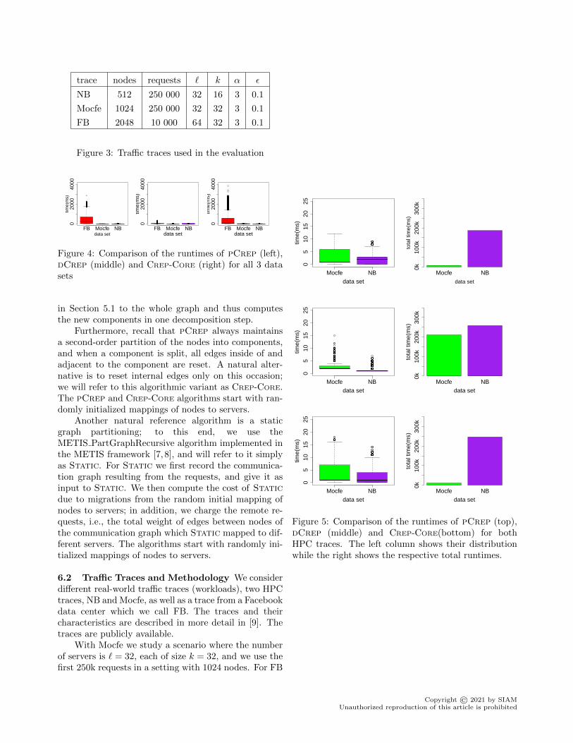
trace nodes requests ` k α ε

NB 512 250 000 32 16 3 0.1

Mocfe 1024 250 000 32 32 3 0.1

FB 2048 10 000 64 32 3 0.1

Figure 3: Traffic traces used in the evaluation

FB Mocfe NB

020

0040

00

data set

time(

ms)

FB Mocfe NB

020

0040

00

data set

time(

ms)

FB Mocfe NB

020

0040

00

data set

time(

ms)

Figure 4: Comparison of the runtimes of pCrep (left),dCrep (middle) and CREP-CORE (right) for all 3 datasets

in Section 5.1 to the whole graph and thus computesthe new components in one decomposition step.

Furthermore, recall that pCrep always maintainsa second-order partition of the nodes into components,and when a component is split, all edges inside of andadjacent to the component are reset. A natural alter-native is to reset internal edges only on this occasion;we will refer to this algorithmic variant as CREP-CORE.The pCrep and CREP-CORE algorithms start with ran-domly initialized mappings of nodes to servers.

Another natural reference algorithm is a staticgraph partitioning; to this end, we use theMETIS PartGraphRecursive algorithm implemented inthe METIS framework [7, 8], and will refer to it simplyas Static. For Static we first record the communica-tion graph resulting from the requests, and give it asinput to Static. We then compute the cost of Staticdue to migrations from the random initial mapping ofnodes to servers; in addition, we charge the remote re-quests, i.e., the total weight of edges between nodes ofthe communication graph which Static mapped to dif-ferent servers. The algorithms start with randomly ini-tialized mappings of nodes to servers.

6.2 Traffic Traces and Methodology We considerdifferent real-world traffic traces (workloads), two HPCtraces, NB and Mocfe, as well as a trace from a Facebookdata center which we call FB. The traces and theircharacteristics are described in more detail in [9]. Thetraces are publicly available.

With Mocfe we study a scenario where the numberof servers is ` = 32, each of size k = 32, and we use thefirst 250k requests in a setting with 1024 nodes. For FB

Mocfe NB

05

1015

2025

data set

time(

ms)

Mocfe NBdata set

tota

l tim

e(m

s)

0k10

0k20

0k30

0k

Mocfe NB

05

1015

2025

data set

time(

ms)

Mocfe NBdata set

tota

l tim

e(m

s)0k

100k

200k

300k

Mocfe NB

05

1015

2025

data set

time(

ms)

Mocfe NBdata set

tota

l tim

e(m

s)0k

100k

200k

300k

Figure 5: Comparison of the runtimes of pCrep (top),dCrep (middle) and CREP-CORE(bottom) for bothHPC traces. The left column shows their distributionwhile the right shows the respective total runtimes.


we restrict the trace to 2048 nodes. For this restrictionwe iteratively chose the vertex pairs that communicatethe most during the first 20 million requests until wereached the number of 2048 nodes; we then added allrequests between two of these nodes to our data set.For this scenario, we used a configuration with ` = 64servers is ` = 32 of size k = 32. The runs are thenperformed on the first 10k of these requests. Similarlywe restricted NB to 512 nodes and used the first 250krequests for this setting; this data set is then evaluatedin a scenario where the number of servers is ` = 32,each of size k = 32. For all configurations we use α = 3and ε = 0.1. These configurations are summarized inFigure 3. The influence of α on the running time isinvestigated further in Section 6.3.

6.3 Runtime Evaluation We evaluate the runningtime of pCrep by considering different traces andalternative algorithms.

Figure 4 shows the results of all data sets for pCrepand dCrep. Here we filtered the running times to onlyinclude updates which have led the respective algorithmto update, i.e. those updates where the communicatingnodes belonged to different components at the time ofthe request. We can see that for pCrep and CREP-CORE

FB produces by far the highest runtime and thatdCrep performs significantly better than pCrep andCREP-CORE for FB. We first compare the runtimes ofthe three algorithms for the HPC data sets before wediscuss the runtimes for FB in greater detail.

Figure 5 shows plots of runtimes of pCrep, dCrepand CREP-CORE for the HPC traces. On the left of thefigure, we can see the distribution of the update timesover the requests while the total times are shown onthe right. The figure shows that pCrep is the fastestfor both HPC traces while CREP-CORE is faster thandCrep. This indicates that the decomposition tree datastructure which both pCrep and CREP-CORE use maybe a significant advantage for the HPC traces.

Figure 6 illustrates the relation of the time neededfor handling a request, and the number of edges in thedata structure for pCrep and for CREP-CORE for FB.We can see a high correlation, i.e., a large number ofedges in the graph maintained by the respective algo-rithm seems to lead to longer update times. Similarlythe update times are shorter after the number of edgesdecreases, i.e. after a component split. While we cannotprove this, we suspect that this may be due to the factthat the data used for the run shows little structure, andthus leads to a large number of (costly) recomputationsteps for our data structure. This is also supported bythe fact that dCrep is significantly faster for FB as onecan see in Figure 4.

0 2000 6000 10000

020

0040

00

request number

time(

ms)

/ #ed

ges

timeedge number

0 2000 6000 10000

020

0040

00

request number

time(

ms)

/ #ed

ges

timeedge number

Figure 6: Relation of size to time for FB for pCrep(left) and CREP-CORE (right)

1 2 4 8 16

020

4060

αtim

e(m

s)α

time(

ms)

1 4 8 16

10k

40k

70k

100k

1 2 4 8 16

010

3050

α

time(

ms)

α

time(

ms)

1 4 8 16

10k

40k

70k

100k

Figure 7: Runtime of pCrep (top) and CREP-CORE

(bottom) for Mocfe for different values of α. The leftcolumn shows their distribution while the right showsthe respective total runtimes.

It is also interesting to study the influence ofα on the running time of pCrep and CREP-CORE.Figure 7 shows plots of the running time of pCrepand CREP-CORE for α ∈ 1, 2, 4, 8, 16. In order toimprove the readability, only requests which led to anupdate of the data structure are included. The resultsshow that for both algorithms the runtimes increase forincreasing values of α. This may be due to the factthat higher values of α lead the algorithms to updatethe tree structure less frequently and thus also to deletecomponents less frquently. This increases the size of thedata structure, making updates slower.

6.4 Cost Evaluation In order to shed light on thecost, in terms of communication and migration, wecompare our algorithms pCrep and CREP-CORE withStatic.

Figure 8 shows the costs of pCrep, CREP-CORE and


FB Mocfe NBdata set

cost

0k15

0k35

0k communication costmigration cost

FB Mocfe NBdata set

cost

0k15

0k35


FB Mocfe NBdata set

cost

0k15

0k35


Figure 8: Comparison of the costs of pCrep (left),CREP-CORE (middle) and Static (right) for all 3 datasets

Static for FB, Mocfe and NB. Note that for FB thecosts of pCrep and CREP-CORE are actually lower thanthe cost of Static. For the HPC traces Static is ableto achieve significantly lower cost than both pCrep andCREP-CORE. However, it is important to keep in mindthat Static is essentially an offline algorithm, whichknows requests ahead of time; furthermore, we alsonote that Static may not produce a perfectly balancedpartitioning.

7 Related Work

The closest work to ours is by Avin et al. [2, 4, 10]who initiated the study of the dynamic balanced graphpartitioning problem. The authors present pCrep,a O(k log k)-competitive algorithm with augmentation2 + ε for any ε > 1/k; this algorithm however hasa super-polynomial runtime, which we improve uponin this paper. In their paper, Avin et al. also showa lower bound of k − 1 for the competitive ratio ofany online algorithm on two clusters via a reductionto online paging; the lower bound was later generalizedby Pacut et al. to Ω(k`) [11].

Restricted variants of the balanced repartitioningproblem have also been studied. Here one assumescertain restrictions of the input sequence σ and thenstudies online algorithms for these cases. In thiscontext, Avin et al. [12, 13] assume that an adversaryprovides requests according to a fixed distribution ofwhich the optimal algorithm OPT has knowledge whilean online algorithm that is compared with OPT hasnot. Further the authors restrict the communicationpattern to form a ring-like pattern, i.e. for the case ofn nodes 0, ..., n − 1 only requests r of the form r = imod n, (i + 1) mod n are allowed. For this case theypresent a competitive online algorithm which achieves acompetitive ratio of O(log n) with high probability.

Henzinger et al. [14] study a special learning vari-ant of the problem where it is assumed that the inputsequence σ eventually reveals a perfect balanced parti-tioning of the n nodes into ` parts of size k such thatthe edge cut is zero. In this case the communication

patterns reveal connected components of the commu-nication graph of which each forms one of the parti-tions. Algorithms are tasked to learn this partition andto eventually collocate nodes according to the partitionwhile minimizing communication and migration costs.The authors of [14] present an algorithm for the casewhere the number of servers is ` = 2 that achieves acompetitive ratio of O((log n)/ε) with augmentation ε,i.e. each server has capacity (1 + ε)n/2 for ε ∈ (0, 1).For the general case of ` servers of capacity (1 + ε)n/`the authors construct an exponential-time algorithmthat achieves a competitive ratio of O((` log n log `)/ε)for ε ∈ (0, 1/2) and also provide a distributed ver-sion. Additionally the authors describe a polynomial-time O((`2 log n log `)/ε2)-competitive algorithm for thecase with general `, servers of capacity (1 + ε)n/` andε ∈ (0, 1/2).

In a recent follow-up work, Henzinger et al. (atSODA 2021) [15] improve upon their results and presentdeterministic and randomized algorithms which achieve(almost) tight bounds for the learning variant of theonline graph partitioning problem. In particular,they present a polynomial-time randomized algorithmachieving a polylogarithmic competitive ratio: they de-rive an O(log `+ log k) upper bound on the competitiveratio of their algorithm, where ` is the number of serversand k is the server capacity, and show that no random-ized online algorithm can achieve a competitive ratio ofless than Ω(log ` + log k). For the deterministic learn-ing variant with no resource augmentation, Pacut et al.showed a tight bound of Θ(k · l) in [11].

The dynamic balanced graph partitioning problemcan be seen as a generalization (or symmetric version)of online paging. In the online paging problem [16], [17]one is given a scenario with a fast cache of k pages andn− k pages in slow memory. Pages are requested in anonline manner, i.e. without prior knowledge of futurerequests. If a requested page is in the cache at the timeof the request it can be served without cost. If it is inslow memory however, then a page fault occurs and therequested page needs to be moved into the cache. Ifthe cache is full then a page from the cache needs tobe evicted, i.e. moved to the slow memory in order tomake space for the requested one. The goal is to designalgorithms which minimize the number of such pagefaults. However, the standard version of online paginghas no equivalent to the option of serving a requestremotely as is possible in the Dynamic Balanced GraphPartitioning problem. The variant with bypassing allowsan algorithm to access pages in slow memory withoutmoving them into the cache, thus providing such anequivalent. It is worth stressing however that in ourproblem requests involve two nodes while in Online


Paging the nodes themselves are requested.The static balanced graph partitioning problem is

the static offline variant of the problem of this paper.In this version an algorithm may not perform anymigrations, but has perfect knowledge of the requestsequence σ and then needs to provide a perfectlybalanced partitioning of the n = k ·` nodes into ` sets ofequal size k that minimizes cost, i.e. the weight of edgesbetween the servers. This scenario can be modelled asa graph partitioning problem where the weight of anedge corresponds to the number of requests betweenits end points in the input sequence σ. An algorithmthen has to provide a partition of the nodes into setsof exactly k nodes each while minimizing the total edgeweights between partitions, i.e. an algorithm needs tominimize the edge cut of the graph. This problem is NP-complete ( [18]) and for the case where ` ≥ 3, Andreevand Racke [18] have shown that there is no polynomialtime approximation algorithm which guarantees a finiteapproximation factor unless P=NP.

There are several algorithms and frameworks forgraph partitioning problems. Usually these frameworksemploy heuristics in order to achieve their results. Themost successful such heuristic is Multilevel Graph Parti-tioning [19]. This method consists of three phases. Ini-tially the graph is repeatedly coarsened into a hierarchyof smaller graphs in such a way that cuts in the coarsegraphs also correspond to cuts in the finer graphs. Onthe coarsest level a (potentially expensive) algorithm isused in order to compute an initial partition. This par-titioning is then transferred to the finer graphs. In thisprocess one usually uses other local heuristics in orderto improve the partition quality even further with everystep. METIS [7,8] and Jostle [20,21] are examples of li-braries that utilize this multilevel approach. We chooseMETIS as a reference for our empirical evaluation.

More generally, clustering has been studied within avariety of different contexts from data mining to imagesegmentation [22,23,24], and is the process of generatingsubsets of elements with high similarity [25]. However,we consider an online problem, i.e. algorithms need toreact dynamically to changes in the graph and need tomaintain their data structures and adapt accordinglywhereas clustering considers complete data sets whichare static.

8 Future Work

While our algorithm does not only achieve a polyno-mial runtime and an almost competitive ratio (up to alogarithmic factor), our work leaves upon several inter-esting directions for future research. On the theoreticalfront, it would be interesting to explore how to closethe gap between upper and lower bound on the com-

petitive ratio, and to study randomized algorithms. Onthe practical front, we believe that our algorithm canbe further engineered and optimized to achieve a lowerruntime in practice, as well as an improved empiricalcompetitive ratio under real (non worst-case) workloads.These kinds of adjustments may be achieved for exam-ple by changing certain algorithm parameters such asthe connectivity threshold. There may also be poten-tial in adapting and improving our decomposition treedata structure in order to improve running times.

References

[1] J. C. Mogul and L. Popa, “What we talk aboutwhen we talk about cloud network performance,” ACMSIGCOMM Computer Communication Review, vol. 42,p. 44, sep 2012.

[2] C. Avin, A. Loukas, M. Pacut, and S. Schmid, “On-line Balanced Repartitioning,” in Proc. 30th Interna-tional Symposium on Distributed Computing (DISC),pp. 243–256, Springer Berlin Heidelberg, 2016.

[3] T. Forner, “Repartitioning Implementation,” GitHub,2020.

[4] C. Avin, M. Bienkowski, A. Loukas, M. Pacut, andS. Schmid, “Dynamic Balanced Graph Partitioning,”arXiv preprint arXiv:1511.02074v5, 2015.

[5] M. Stoer and F. Wagner, “A simple min-cut algo-rithm,” Journal of the ACM, vol. 44, pp. 585–591, jul1997.

[6] L. Chang, J. X. Yu, L. Qin, X. Lin, C. Liu, andW. Liang, “Efficiently computing k-edge connectedcomponents via graph decomposition,” in Proceedingsof the 2013 international conference on Managementof data - SIGMOD '13, ACM Press, 2013.

[7] G. Karypis and V. Kumar, “A fast and high qualitymultilevel scheme for partitioning irregular graphs,”SIAM Journal on Scientific Computing, vol. 20,pp. 359–392, jan 1998.

[8] G. Karypis and V. Kumar, “Multilevelk-way partition-ing scheme for irregular graphs,” Journal of Paralleland Distributed Computing, vol. 48, pp. 96–129, jan1998.

[9] C. Avin, M. Ghobadi, C. Griner, and S. Schmid,“Measuring the Complexity of Packet Traces,”arXiv:1905.08339v1, 2019.

[10] C. Avin, M. Bienkowski, A. Loukas, M. Pacut, andS. Schmid, “Dynamic balanced graph partitioning,” inSIAM J. Discrete Math (SIDMA), 2019.

[11] M. Pacut, M. Parham, and S. Schmid, “Brief an-nouncement: Deterministic lower bound for dynamicbalanced graph partitioning,” in Proc. ACM Sympo-sium on Principles of Distributed Computing (PODC),2020.

[12] C. Avin, L. Cohen, and S. Schmid, “Competitiveclustering of stochastic communication patterns onthe ring,” in Proc. 5th International Conference onNetworked Systems (NETYS), 2017.


[13] C. Avin, L. Cohen, M. Parham, and S. Schmid,“Competitive clustering of stochastic communicationpatterns on a ring,” Computing, vol. 101, pp. 1369–1390, sep 2018.

[14] M. Henzinger, S. Neumann, and S. Schmid, “Effi-cient Distributed Workload (Re-)Embedding,” no idea,2019.

[15] M. Henzinger, S. Neumann, H. Raecke, and S. Schmid,“Tight bounds for online graph partitioning,” inProc. ACM-SIAM Symposium on Discrete Algorithms(SODA), 2021.

[16] A. Fiat, R. Karp, M. Luby, L. McGeoch, D. Sleator,and N. E. Young, “Competitive Paging Algorithms,”arXiv preprint cs/0205038, 2002.

[17] L. Epstein, C. Imreh, A. Levin, and J. Nagy-Gyorgy,“On variants of file caching,” in Automata, Languagesand Programming, pp. 195–206, Springer Berlin Hei-delberg, 2011.

[18] K. Andreev and H. Racke, “Balanced Graph Partition-ing,” Theory of Computing Systems, vol. 39, pp. 929–939, oct 2006.

[19] A. Buluc, H. Meyerhenke, I. Safro, P. Sanders, andC. Schulz, “Recent Advances in Graph Partitioning,”in Algorithm Engineering, pp. 117–158, Springer Inter-national Publishing, 2016.

[20] C. Walshaw and M. Cross, “Mesh partitioning: Amultilevel balancing and refinement algorithm,” SIAMJournal on Scientific Computing, vol. 22, pp. 63–80,jan 2000.

[21] C. Walshaw and M. Cross, “JOSTLE: parallel multi-level graph-partitioning software–an overview,” Meshpartitioning techniques and domain decomposition tech-niques, pp. 27–58, 2007.

[22] A. C. Benabdellah, A. Benghabrit, and I. Bouhad-dou, “A survey of clustering algorithms for an indus-trial context,” Procedia Computer Science, vol. 148,pp. 291–302, 2019.

[23] Z. Wu and R. Leahy, “An optimal graph theoretic ap-proach to data clustering: theory and its applicationto image segmentation,” IEEE Transactions on Pat-tern Analysis and Machine Intelligence, vol. 15, no. 11,pp. 1101–1113, 1993.

[24] M. Pavan and M. Pelillo, “A new graph-theoretic ap-proach to clustering and segmentation,” in 2003 IEEEComputer Society Conference on Computer Vision andPattern Recognition, 2003. Proceedings., IEEE Com-put. Soc, 2003.

[25] E. Hartuv and R. Shamir, “A clustering algorithmbased on graph connectivity,” Information ProcessingLetters, vol. 76, pp. 175–181, dec 2000.

A Deferred Technical Details

The proofs of the following claims are omitted due tospace constraints.

Lemma A.1. At any time t after pCrep performed itsmerge and split actions, all subsets S of componentswith |S| > 1 have connectivity less than α, i.e. there ex-ist no mergeable component sets after pCrep performedits merges and splits.

The following lemma is adapted for ourconnectivity-based approach from Corollary 4.2in [4].

Lemma A.2. Fix any time t and consider weights rightafter they were updated by pCrep but before any mergeor split actions. Then all subsets S of components with|S| > 1 have connectivity at most α and a mergeablecomponent set S has connectivity exactly α.

The following two lemmas combined give us a resultsimilar to Lemma 4.3 in [4]: bounds on the edge weightthat is cut when partitioning a mergeable componentset, i.e. a set of components of connectivity at least α.

We start by establishing a lower bound on this edgeweight in the following lemma.

Lemma A.3. Given a mergeable set of components Sand a partition of S into g > 1 parts S1, ..., Sg. Thenthe weight between the parts of the partition is at leastg/2 · α.

In the following lemma we establish the upperbound on the cut edge weight when partitioning amergeable set of components S into g ≥ 2 parts.

Lemma A.4. Given a mergeable set of components Sand a partitioning of S into g ≥ 2 parts S1, ..., Sg. Theweight between the parts Si is at most (g− 1) ·α duringthe execution of pCrep.


Online Balanced Repartitioning of Dynamic Communication ...

Documents

Transcript of Online Balanced Repartitioning of Dynamic Communication ...