Online Assessment of Landing Sites
14
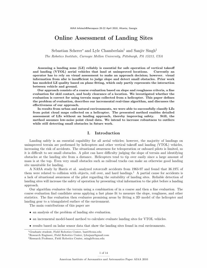
AIAA Infotech@Aerospace 20-22 April 2010, Altanta, Georgia Online Assessment of Landing Sites Sebastian Scherer ∗ and Lyle Chamberlain † and Sanjiv Singh ‡ The Robotics Institute, Carnegie Mellon University, Pittsburgh, PA 15213, USA Assessing a landing zone (LZ) reliably is essential for safe operation of vertical takeoff and landing (VTOL) aerial vehicles that land at unimproved locations. Currently an operator has to rely on visual assessment to make an approach decision; however. visual information from afar is insufficient to judge slope and detect small obstacles. Prior work has modeled LZ quality based on plane fitting, which only partly represents the interaction between vehicle and ground. Our approach consists of a coarse evaluation based on slope and roughness criteria, a fine evaluation for skid contact, and body clearance of a location. We investigated whether the evaluation is correct for using terrain maps collected from a helicopter. This paper defines the problem of evaluation, describes our incremental real-time algorithm, and discusses the effectiveness of our approach. In results from urban and natural environments, we were able to successfully classify LZs from point cloud maps collected on a helicopter. The presented method enables detailed assessment of LZs without an landing approach, thereby improving safety. Still, the method assumes low-noise point cloud data. We intend to increase robustness to outliers while still detecting small obstacles in future work. I. Introduction Landing safely is an essential capability for all aerial vehicles; however, the majority of landings on unimproved terrain are performed by helicopters and other vertical takeoff and landing (VTOL) vehicles, increasing the risk of accidents. The situational awareness for teleoperation or onboard pilots is limited, so it is difficult to see small obstacles. A pilot can have difficulty judging the slope of terrain and identifying obstacles at the landing site from a distance. Helicopters tend to tip over easily since a large amount of mass is at the top. Even very small obstacles such as railroad tracks can make an otherwise good landing site unsuitable for landing. A NASA study by Harris et al. analyzed rotorcraft accidents from 1963-97 and found that 36.19% of them were related to collision with objects, roll over, and hard landings. 1 A partial cause for accidents is a lack of situational awareness of the pilot regarding the suitability of landing sites. Reliable detection of landing sites will increase the safety of operation by presenting vital information to the pilot before a landing approach. Our algorithm evaluates the terrain using a combination of in a coarse and then a fine evaluation. The coarse evaluation find candidate areas applying a fast plane fit to measure the slope, roughness, and other statistics. The fine evaluation then evaluates promising areas by fitting a 3D model of the helicopter and landing gear to a triangulated surface of the environment. The main contributions of this paper are • an analysis of the problem of landing site evaluation. • an incremental model-based method to calculate evaluate landing sites for VTOL vehicles. • results based on ladar sensor data that show the landing sites found in real environments. ∗ Graduate student, Field Robotics Center, [email protected] † Research Engineer, Field Robotics Center, [email protected] ‡ Research Professor, Field Robotics Center, [email protected] 1 of 14 American Institute of Aeronautics and Astronautics Paper AIAA 2010
Transcript of Online Assessment of Landing Sites
AIAA Infotech@Aerospace 20-22 April 2010, Altanta, Georgia
Online Assessment of Landing Sites
Sebastian Scherer∗ and Lyle Chamberlain† and Sanjiv Singh‡
The Robotics Institute, Carnegie Mellon University, Pittsburgh, PA 15213, USA
Assessing a landing zone (LZ) reliably is essential for safe operation of vertical takeoff
and landing (VTOL) aerial vehicles that land at unimproved locations. Currently an
operator has to rely on visual assessment to make an approach decision; however. visual
information from afar is insufficient to judge slope and detect small obstacles. Prior work
has modeled LZ quality based on plane fitting, which only partly represents the interaction
between vehicle and ground.
Our approach consists of a coarse evaluation based on slope and roughness criteria, a fine
evaluation for skid contact, and body clearance of a location. We investigated whether the
evaluation is correct for using terrain maps collected from a helicopter. This paper defines
the problem of evaluation, describes our incremental real-time algorithm, and discusses the
effectiveness of our approach.
In results from urban and natural environments, we were able to successfully classify LZs
from point cloud maps collected on a helicopter. The presented method enables detailed
assessment of LZs without an landing approach, thereby improving safety. Still, the
method assumes low-noise point cloud data. We intend to increase robustness to outliers
while still detecting small obstacles in future work.
I. Introduction
Landing safely is an essential capability for all aerial vehicles; however, the majority of landings onunimproved terrain are performed by helicopters and other vertical takeoff and landing (VTOL) vehicles,increasing the risk of accidents. The situational awareness for teleoperation or onboard pilots is limited, soit is difficult to see small obstacles. A pilot can have difficulty judging the slope of terrain and identifyingobstacles at the landing site from a distance. Helicopters tend to tip over easily since a large amount ofmass is at the top. Even very small obstacles such as railroad tracks can make an otherwise good landingsite unsuitable for landing.
A NASA study by Harris et al. analyzed rotorcraft accidents from 1963-97 and found that 36.19% ofthem were related to collision with objects, roll over, and hard landings.1 A partial cause for accidents isa lack of situational awareness of the pilot regarding the suitability of landing sites. Reliable detection oflanding sites will increase the safety of operation by presenting vital information to the pilot before a landingapproach.
Our algorithm evaluates the terrain using a combination of in a coarse and then a fine evaluation. Thecoarse evaluation find candidate areas applying a fast plane fit to measure the slope, roughness, and otherstatistics. The fine evaluation then evaluates promising areas by fitting a 3D model of the helicopter andlanding gear to a triangulated surface of the environment.
The main contributions of this paper are
• an analysis of the problem of landing site evaluation.
• an incremental model-based method to calculate evaluate landing sites for VTOL vehicles.
• results based on ladar sensor data that show the landing sites found in real environments.∗Graduate student, Field Robotics Center, [email protected]†Research Engineer, Field Robotics Center, [email protected]‡Research Professor, Field Robotics Center, [email protected]
1 of 14
American Institute of Aeronautics and Astronautics Paper AIAA 2010

This paper first reviews related work, details our approach, and then presents results for the landing siteevaluation algorithm.
Where is a good
landing zone?
Point CloudOverhead Image
Figure 1: The problem addressed in this paper is to find good landing zones for rotary wing vehicles. Onthe left is an overhead image for reference. The input to the algorithm is an incrementally updated pointcloud that is evaluated to find suitable landing zones.
II. Related Work
There has been some prior work on landing and landing site selection. From a control perspective theproblem has been studied by Sprinkle2 to determine if a trajectory is still feasible to land. Saripalli et al.3,4have landed on a moving target that was known to be a good landing site. Barber et al.5 used optical flowbased control to control a fixed wing vehicle to land.
Vision has been a more popular sensor modality for landing site evaluation because the sensor is lightweight.De Wagter and Mulder6 describe a system that uses vision for control, terrain reconstruction, and tracking.A camera is used to estimate the height above ground for landing in Yu et al.,7 and similarly in Meijas etal.8 a single camera is used to detect and avoid powerlines during landing.
Using a stereo camera, Hintze9 developed an algorithm to land in unknown environments. Bosch et al.propose an algorithm for monocular images that is based on detecting nonplanar regions to distinguish land-ing sites from non-landing sites.10 Another popular approach is to use structure from motion to reconstructthe motion of the camera and to track sparse points that allow reconstruction of the environment and planefitting. This method as been applied to spacecraft by Johnson et al.11 and to rotor craft by Templeton etal.12
Ladar based landing site evaluation has not been studied very deeply except as suggested in Serrano etal.13 where a framework for multiple sources like ladar, radar, and cameras is proposed to infer the suitabilityof a landing site. For ground vehicles ladar based classification is popular because of its reliability and directrange measurement. It has been used in conjunction with aerial vehicle data for ground vehicles by Sofmanet al.14 and by Hebert & Vandapel.15
Our work in landing site evaluation uses ladar data and some of the proposed techniques in related worksuch as plane fitting and roughness. However, our method goes beyond pure plane fitting to actually fit amodel of the helicopter geometry to a triangulation of the environment.
III. Problem
The suitability of a landing zone depends to a large degree on the characteristics of the aircraft that will belanding on it. We consider larger vehicles such as manned helicopters, however the problem scales to smalleraircraft. Landing of a helicopter can roughly be separated into two independent phases: an approach, anda ground contact. During the approach, the helicopter ideally keeps a steady and relatively shallow descentangle in a straight line to come to a hover at some altitude above the ground. Then it orients with respectto the ideal location on the ground and touches down.
2 of 14
American Institute of Aeronautics and Astronautics Paper AIAA 2010
Assessment of a LZ needs to include two main factors: the ground conditions and the approach conditions.The ground conditions are all factors that are relevant when the aircraft is contact with the ground, whilethe approach conditions are related to moving to the LZ.
The ground conditions that need to be considered for assessing an LZ are
• minimum size of the site
• skid contact
• static stability on ground based on the center of gravity of the aircraft
• load bearing capability of the contact surface
• loose foreign objects (FOD) and vegetation surrounding the site
• clearance of aircraft/rotor with surrounding terrain and objects
To ensure a reliable and successful landing it is necessary to consider all these factors in a landing siteevaluation algorithm. However some factors such as the load bearing capability, and foreign objects aredifficult to classify purely based on the geometric approach that we use. In our approach we assume thata geometrically good site will be able to hold the load of the helicopter and FOD objects will be classifiedas sufficient roughness to cause a rejection. Future work will also incorporate approach and abort paths forflying a landing pattern.
IV. Approach
Sorted list
of good
landing sites
(x,y, )!
Coarse
Evaluation
Point Cloud (x,y,z)
Fine
Evaluation
List of potential
landing location (x,y)
Combination
TriangulationTerrain Grid Map
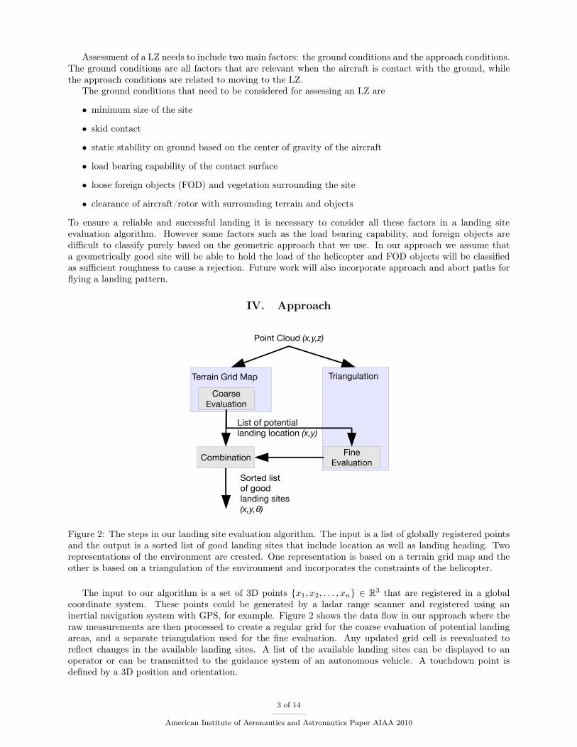
Figure 2: The steps in our landing site evaluation algorithm. The input is a list of globally registered pointsand the output is a sorted list of good landing sites that include location as well as landing heading. Tworepresentations of the environment are created. One representation is based on a terrain grid map and theother is based on a triangulation of the environment and incorporates the constraints of the helicopter.
The input to our algorithm is a set of 3D points {x1, x2, . . . , xn} ∈ R3 that are registered in a globalcoordinate system. These points could be generated by a ladar range scanner and registered using aninertial navigation system with GPS, for example. Figure 2 shows the data flow in our approach where theraw measurements are then processed to create a regular grid for the coarse evaluation of potential landingareas, and a separate triangulation used for the fine evaluation. Any updated grid cell is reevaluated toreflect changes in the available landing sites. A list of the available landing sites can be displayed to anoperator or can be transmitted to the guidance system of an autonomous vehicle. A touchdown point isdefined by a 3D position and orientation.
3 of 14
American Institute of Aeronautics and Astronautics Paper AIAA 2010

A. Coarse Evaluation
The first step in our algorithm is a coarse evaluation of a regular terrain grid map. Each cell in the map,roughly the size of the landing gear, tests how the vehicle would come into contact with the ground. Themap keeps a set of statistics in a two dimensional hash table of cells. The hash key is calculated based onthe point coordinate at a fixed resolution. This provides a naturally scrolling implementation and cells canbe set as data are measured. As the vehicles moves and the map scrolls, old cells will be overwritten. Thisdata structure allows the algorithm to quickly add new data to the map. Each cell in the grid keeps a set ofstatistics: The mean, minimum, and maximum z-value, the number of points, and the moments necessaryto calculate the plane fit.
For Each
Patch
Are all binary
Attributes valid?Bad Landing
SiteNoReturn
GoodnessYesCalculate the
goodness
Fit Plane to
Patch
Figure 3: A flow chart showing the control flow of evaluating a patch in the terrain grid map. Only if allbinary attributes shown in table 1 are valid a landing zone will be considered.
# Description Symbol Operator Value
1 Do we have more than x points for a plane fit? c > 152 Is the spread of the points less than x cm? σn < 503 Was the plane fit successful? = True4 Is the residual for the plane fit less than x? r < 45 Is the slope of the plane less than x degrees? α < 5
Table 1: The binary attributes considered in the rough evaluation for landing site evaluation. Only if alloperations evaluate to true a landing site can be available.
The statistics accumulated in each terrain cell are evaluated to assess a particular location. Based on thesetests a series of binary attributes and goodness values can be computed. The statistics can be accumulatedwith neighboring cells which allows us to compute the suitability of larger regions. The binary tests aredesigned to reject places where the ground is too rough or too step to be valid; furthermore, the algorithmcannot make a reliable estimate of a landing site, if not enough data is available.
The binary attributes are computed as follows: First, we check if enough points are available to performa plane fit. We require at least 15 points per cell, which is an average density of one point every 20 cm fora 3 m cell. This average density is the required density for the smallest obstacle we consider; however, wemake an optimistic assumption since points are not necessarily distributed evenly. Next, we consider thestandard deviation of the z-value. The algorithm rejects cells if the vertical standard deviation is larger than50 cm, rejecting any area with large altitude changes. The value has to be large enough to avoid interferingwith the results of the plane fitting since a large change in altitude also characterizes a large slope. Finally,the slope and residual of a plane fit are checked for a planar surface. The residual will be a good indicatorfor the roughness of the terrain since it measures deviation from the plane. Currently the slope threshold isset at 5 degrees and the residual threshold is set at 4.
The mean altitude and standard deviation of the plane is calculated based on Welford’s algorithm bykeeping the mean and the corrected sum of squares.16 After receiving a new altitude measurement in a patchthe mean altitude µc and sum of squares Sc are updated:
4 of 14
American Institute of Aeronautics and Astronautics Paper AIAA 2010

µnew = µc−1 + (z − µc−1)/n (1)
Sc = Sc−1 + (z − µc−1) · (z − µnew) (2)
µc = µnew
The standard deviation σ can be calculated from S as follows:
σc =�
Sc
c(3)
Additionally we want to evaluate the slope and need to fit a plane with respect to the measurements. Afast algorithm to calculate a least squares plane fit is a moment based calculation. The fit is a least squaresfit along z and therefore assumes no errors in x and y exist (Also see Templeton et al.17). We only have tokeep track of the moments
M =
Mxx Mxy Mxz
Mxy Myy Myz
Mxz Myz Mzz
(4)
and the offset vector
Mo =
Mx
My
Mz
(5)
and the number of total points c. The moments can be updated for a new measurement (x, y, z) byupdating the moments starting from 0 for all initial values.
Mx = Mx + x, My = My + y, Mz = Mz + z (6)
Mxx = Mxx + x2, Myy = Myy + y2, Mzz = Mzz + z2 (7)
Mxy = Mxy + x · y, Mxz = Mxz + x · z, Myz = Myz + y · z (8)
c = c + 1 (9)
Consequently, an update is the constant time required to update the 10 values and the plane fit iscalculated in closed form. Another advantage is that we can accumulate the moments from the neighboringcells to fit a larger region in the terrain that represents the whole area of the helicopter, not just the landing
skids. See Ahn18 for more details on moment based fitting. The plane normal n =
A
B
C
and residual r
are calculate as such:
Mn = (M2xyc− 2 · MxMxyMy,+M2
xMyy + (M2y − cMyy)Mxx (10)
A = (M2y Mxz − (MxMyz + MxyMz)My + c(−MxzMyy + MxyMyz) + XxMY Y Mz)/Mn (11)
B = (−(MxyMz + MxzMy)Mx + cMxyMxz + M2xMyz + Mxx(−cMyz + MyMz)/Mn (12)
C = (−(MxMyz + MxzMy)Mxy + MxMxzMyy + M2xyMz + Mxx(MY Myz −MyyMz))/Mn (13)
r =�
|C2c + 2ACMx + A2Mxx + 2BCMx + 2ABMxy + B2MY Y − 2CMz − 2AMxz − 2BMyz + Mzz| /c
(14)
5 of 14
American Institute of Aeronautics and Astronautics Paper AIAA 2010

We can infer the slope and roughness based on the normal and residual. The slope can be calculated asfollows
α = acos(vTupn) (15)
where vup = (0, 0, −1) is the up vector and n is the plane normal.If all the binary attributes shown in table 1 pass, the algorithm calculates the goodness attributes used in
the final evaluation. All potentially good landing sites are now evaluated with the fine evaluation to decideif touching down is feasible.
B. Fine Evaluation
For Each
Position and
Heading
Too Close to
Ground GoalBad Landing
Site
Good PoseBad Landing
Site
Roll or Pitch
Angle >ThresholdBad Landing
SiteYes
Good Fit of 3D
Model Bad Landing
SiteNo
Return
Goodness of
SiteCalculate Roll,
Pitch and Altitude
Fit 3D Model
Figure 4: The flow chart of the fine evaluation algorithm. The pose of the helicopter is calculated based ona (x, y, θ) position and heading. If the pose is calculated successfully a surface model of the aerial vehicle isevaluated.
Once we have determined a list of general locations, we finely evaluate each potentially good site withrespect to a 2D Delaunay triangulation of all available data. A Delaunay triangulation is a triangular networkof points that can be constructed efficiently (See Preparate & Shamos for more details19). The reason forthis staged processing is that it is easier to know when to incrementally update a cell-based representation,and the incremental calculation for the rough grid is much faster than for the triangulation.
While the rough evaluation considers the plane geometry and roughness of a landing site, the triangulationactually tries to simulate the helicopter coming in contact with the surface. As a first step we incrementallyupdate a hierarchical triangulation with a maximum number of points per patch area. For an implementationsee Fabri et al.20 If the point density is exceeded, we randomly remove points from the triangulation to keepbelow a maximum amount of memory used. Currently, the patch size is set to 3 meters and the maximumpoint density is set to 200 points/cell, which corresponds to an even point spacing of approximately 20cm.
Once the coarse evaluation calculates a list of potential (x, y) locations, the fine evaluation tries to findthe best orientation and determines if the chosen location is feasible. We test a series of possible orientationsθ of the helicopter (8 in our experiments) by intersecting the virtual landing gear with the measured terrainto determine what the resulting pose of the helicopter would be (Also see figure 4). Currently our algorithmonly works for two landing skids, which is a very common configuration of landing gear.
First we determine the intersections of the skids with the triangulation by walking along the two linesrepresenting the landing skids, and extract the height above ground as shown in figure 5. Now we assumethat the helicopter’s center of gravity is on top of the landing skids and calculate the two highest points ofthe intersection. These two points will be the points that determine the position of the skid in the staticcase. We repeat this process for all eight potential landing gear positions.
6 of 14
American Institute of Aeronautics and Astronautics Paper AIAA 2010
0 0.1 0.2 0.3 0.4 0.5 0.6 0.7 0.8 0.9 10
0.1
0.2
0.3
0.4
0.5
0.6
0.7
0.8
0.9
1
x[m]
y[m]
!"#$%&'($)*%+,#-.+/0#12+
3"4$+54-,44%+/0#1+$%1+
6#%4+/4&74%-2+
8*24+*%+9"*'%1:+
;*((+$%1+8#-<.+="*7+/0#12+
8#-<.+3"4$+
/0#1+
!4""$#%+
9**1+>*%-$<-+
?$1+>*%-$<-+
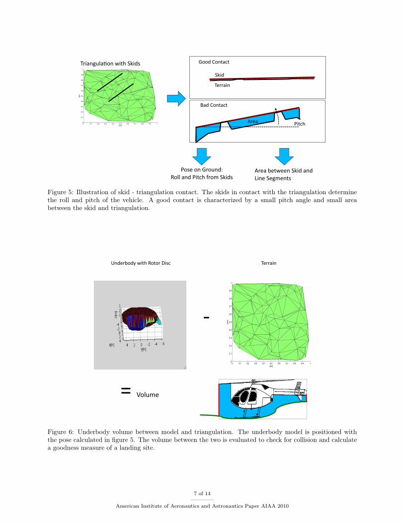
Figure 5: Illustration of skid - triangulation contact. The skids in contact with the triangulation determinethe roll and pitch of the vehicle. A good contact is characterized by a small pitch angle and small areabetween the skid and triangulation.
!"##$%&'(&)"#*+),'-%./'0+.+#'1%23'
0 0.1 0.2 0.3 0.4 0.5 0.6 0.7 0.8 0.9 10
0.1
0.2
0.3
0.4
0.5
0.6
0.7
0.8
0.9
1
x[m]
y[m]4'
5'6+789"'
Figure 6: Underbody volume between model and triangulation. The underbody model is positioned withthe pose calculated in figure 5. The volume between the two is evaluated to check for collision and calculatea goodness measure of a landing site.
7 of 14
American Institute of Aeronautics and Astronautics Paper AIAA 2010
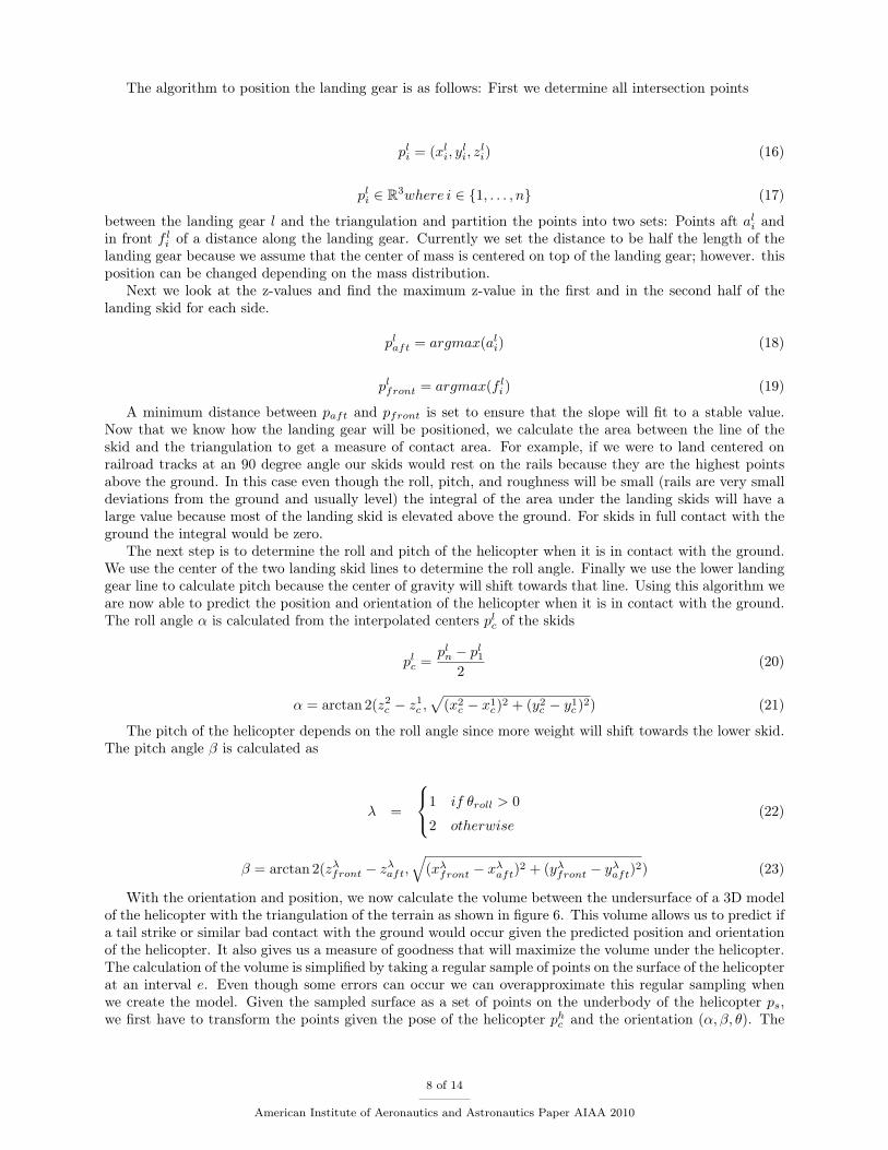
The algorithm to position the landing gear is as follows: First we determine all intersection points
pli = (xl
i, yli, z
li) (16)
pli ∈ R3where i ∈ {1, . . . , n} (17)
between the landing gear l and the triangulation and partition the points into two sets: Points aft ali and
in front f li of a distance along the landing gear. Currently we set the distance to be half the length of the
landing gear because we assume that the center of mass is centered on top of the landing gear; however. thisposition can be changed depending on the mass distribution.
Next we look at the z-values and find the maximum z-value in the first and in the second half of thelanding skid for each side.
plaft = argmax(al
i) (18)
plfront = argmax(f l
i ) (19)
A minimum distance between paft and pfront is set to ensure that the slope will fit to a stable value.Now that we know how the landing gear will be positioned, we calculate the area between the line of theskid and the triangulation to get a measure of contact area. For example, if we were to land centered onrailroad tracks at an 90 degree angle our skids would rest on the rails because they are the highest pointsabove the ground. In this case even though the roll, pitch, and roughness will be small (rails are very smalldeviations from the ground and usually level) the integral of the area under the landing skids will have alarge value because most of the landing skid is elevated above the ground. For skids in full contact with theground the integral would be zero.
The next step is to determine the roll and pitch of the helicopter when it is in contact with the ground.We use the center of the two landing skid lines to determine the roll angle. Finally we use the lower landinggear line to calculate pitch because the center of gravity will shift towards that line. Using this algorithm weare now able to predict the position and orientation of the helicopter when it is in contact with the ground.The roll angle α is calculated from the interpolated centers pl
c of the skids
plc =
pln − pl
1
2(20)
α = arctan 2(z2c − z1
c ,�
(x2c − x1
c)2 + (y2c − y1
c )2) (21)
The pitch of the helicopter depends on the roll angle since more weight will shift towards the lower skid.The pitch angle β is calculated as
λ =
1 if θroll > 0
2 otherwise(22)
β = arctan 2(zλfront − zλ
aft,�
(xλfront − xλ
aft)2 + (yλfront − yλ
aft)2) (23)
With the orientation and position, we now calculate the volume between the undersurface of a 3D modelof the helicopter with the triangulation of the terrain as shown in figure 6. This volume allows us to predict ifa tail strike or similar bad contact with the ground would occur given the predicted position and orientationof the helicopter. It also gives us a measure of goodness that will maximize the volume under the helicopter.The calculation of the volume is simplified by taking a regular sample of points on the surface of the helicopterat an interval e. Even though some errors can occur we can overapproximate this regular sampling whenwe create the model. Given the sampled surface as a set of points on the underbody of the helicopter ps,we first have to transform the points given the pose of the helicopter ph
c and the orientation (α,β, θ). The
8 of 14
American Institute of Aeronautics and Astronautics Paper AIAA 2010
transformed points p�
s are then compared to the intersected point pt of the triangulation. The volume isdefined as
vj =
e2(z
�
s − zt) if z�
s − zt > 0
−∞ otherwise(24)
Vunderbody =m�
j=0
vj (25)
If the underbody surface intersects with the triangulation, the volume becomes −∞ because we have acollision with the terrain.
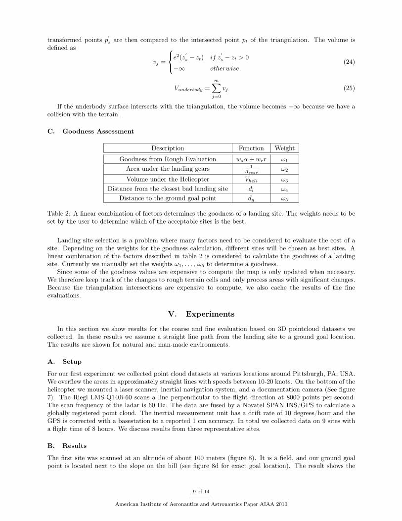
C. Goodness Assessment
Description Function Weight
Goodness from Rough Evaluation wsα + wrr ω1
Area under the landing gears 1Agear
ω2
Volume under the Helicopter Vheli ω3
Distance from the closest bad landing site dl ω4
Distance to the ground goal point dg ω5
Table 2: A linear combination of factors determines the goodness of a landing site. The weights needs to beset by the user to determine which of the acceptable sites is the best.
Landing site selection is a problem where many factors need to be considered to evaluate the cost of asite. Depending on the weights for the goodness calculation, different sites will be chosen as best sites. Alinear combination of the factors described in table 2 is considered to calculate the goodness of a landingsite. Currently we manually set the weights ω1, . . . , ω5 to determine a goodness.
Since some of the goodness values are expensive to compute the map is only updated when necessary.We therefore keep track of the changes to rough terrain cells and only process areas with significant changes.Because the triangulation intersections are expensive to compute, we also cache the results of the fineevaluations.
V. Experiments
In this section we show results for the coarse and fine evaluation based on 3D pointcloud datasets wecollected. In these results we assume a straight line path from the landing site to a ground goal location.The results are shown for natural and man-made environments.
A. Setup
For our first experiment we collected point cloud datasets at various locations around Pittsburgh, PA, USA.We overflew the areas in approximately straight lines with speeds between 10-20 knots. On the bottom of thehelicopter we mounted a laser scanner, inertial navigation system, and a documentation camera (See figure7). The Riegl LMS-Q140i-60 scans a line perpendicular to the flight direction at 8000 points per second.The scan frequency of the ladar is 60 Hz. The data are fused by a Novatel SPAN INS/GPS to calculate aglobally registered point cloud. The inertial measurement unit has a drift rate of 10 degrees/hour and theGPS is corrected with a basestation to a reported 1 cm accuracy. In total we collected data on 9 sites witha flight time of 8 hours. We discuss results from three representative sites.
B. Results
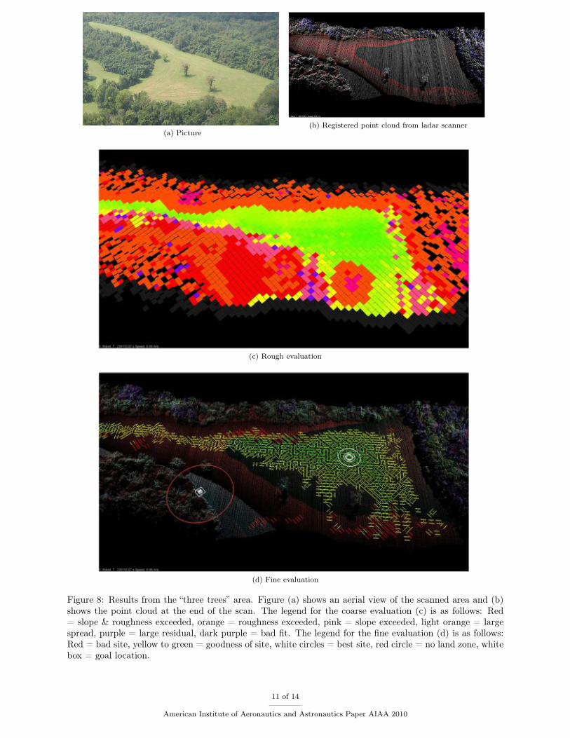
The first site was scanned at an altitude of about 100 meters (figure 8). It is a field, and our ground goalpoint is located next to the slope on the hill (see figure 8d for exact goal location). The result shows the
9 of 14
American Institute of Aeronautics and Astronautics Paper AIAA 2010

(a)
(b)
Figure 7: The experimental setup for data collection for our experiments in Pittsburgh, PA, USA. Wemounted a ladar, and inertial navigation system on a helicopter as shown in figure (a). The sensor platformis shown in figure (b). The inertial measurement unit was located next to the ladar on a shock mount tominimize errors in the registration of the data due to vibration.
coarse and fine evaluation of landing sites in the environment. Several possibly good landing sites in thecoarse evaluation are rejected in the fine evaluation phase. Finally, the best landing site is picked in a spotwith small slope and a large clearance from obstacles.
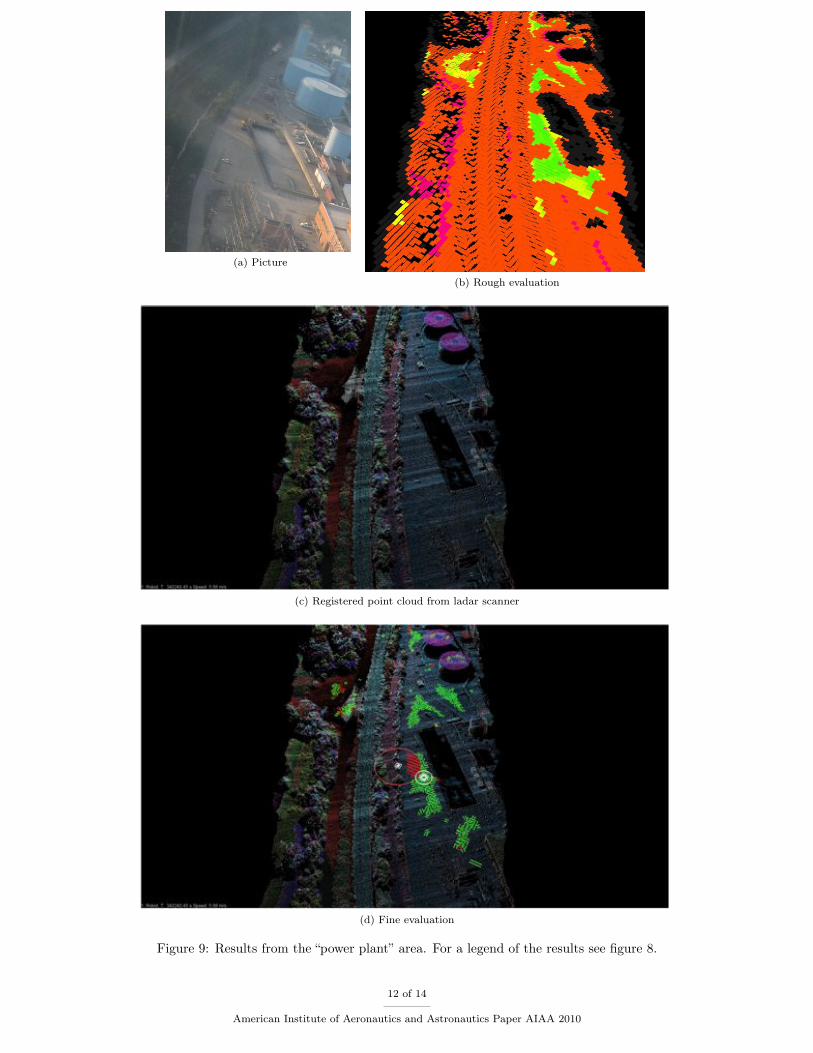
While the previous dataset was mostly in vegetated terrain we also collected a dataset at a coal powerplant (figure 9) at 200m elevation above ground. The geometry of obstacles at the power plant is verydifferent from vegetation, but the algorithm is still able to determine good landing sites. The ground goallocation is close to a car, and one can see how the fine evaluation reject the car and the red region aroundthe ground goal. The red region is a safety buffer that prevents landing directly on top of the ground goal.
As a final experiment, we varied the weights for our evaluation function for four different parameters inthe same terrain (figure 10). First we changed the weight for slope and roughness (figure 10a). Comparedto the nominal evaluation, one can see that we now choose a landing site further away from the ground goalpoint because it is in smoother and less sloped terrain. A similar location is chosen in figure 10b; however,since we try to emphasize the volume of the underbody, the shape of the LZ is actually more convex thanthe evaluation in Fig 10a.
If we give a large weight to the distances to the casualty, we expect the distance to be small. We can seein the evaluation for figure 10c that far points have low weight and close points have the lowest weight. Infigure 10d, the result is almost the same as figure 10c, except that now points close to the boundary also havea low value. Varying the weights, one notices that the weight vector has a large influence on the resultingchosen landing site.
Time(ms) Units
Adding Points 16 /100 pointsCoarse Evaluation 49 /1000 cellsFine Evaluation 26 /cell
Table 3: Computation time for the three parts of the algorithm.
Table 3 shows the computation time required for the different steps in the algorithm on a 2.5 GHz IntelCore 2 Duo. Adding new data is relatively fast and takes currently about 16 ms/100 points which is aboutrealtime for the laser used in the experiments. The data input is designed in such a way that data is droppedif the processing cannot keep up with the ladar data. The coarse evaluation is very fast at 49ms/1000 cells.
10 of 14
American Institute of Aeronautics and Astronautics Paper AIAA 2010
(a) Picture(b) Registered point cloud from ladar scanner
(c) Rough evaluation
(d) Fine evaluation
Figure 8: Results from the “three trees” area. Figure (a) shows an aerial view of the scanned area and (b)shows the point cloud at the end of the scan. The legend for the coarse evaluation (c) is as follows: Red= slope & roughness exceeded, orange = roughness exceeded, pink = slope exceeded, light orange = largespread, purple = large residual, dark purple = bad fit. The legend for the fine evaluation (d) is as follows:Red = bad site, yellow to green = goodness of site, white circles = best site, red circle = no land zone, whitebox = goal location.
11 of 14
American Institute of Aeronautics and Astronautics Paper AIAA 2010
(a) Picture
(b) Rough evaluation
(c) Registered point cloud from ladar scanner
(d) Fine evaluation
Figure 9: Results from the “power plant” area. For a legend of the results see figure 8.
12 of 14
American Institute of Aeronautics and Astronautics Paper AIAA 2010

(a) 1000 · w1 (b) 1000 · w3
(c) 100 · w6 (d) 11000 · w4
Figure 10: This figure shows the result of varying the weights for the final decision on selecting the bestlanding site. For a legend of the results see figure 8. In this plot we keep the function constant and varythe weight for some of the factors described in table 2. In (a) we increase the weight of 1000 · w1 - the slopeand roughness, for (b) we increase 1000 · w3 to emphasize the clearance of the helicopter above the terrain,for (c) we try to minimize the distance to the ground goal by increasing 100 ·w5, and in (d) we decrease theweight of the distance to the closet obstacles by changing 1
1000 · w4. One can see that depending on the costfunction the distribution of good sites changes, as well as the best picked landing site. The weighting doesnot influence the binary decision of acceptable sites because it is based on hard thresholds of the helicoptersconstraints.
This rate corresponds to about 184m2
ms of area covered. The fine evaluation is much slower which justifiesthe coarse evaluation to limit the number of fine evaluations performed.
VI. Conclusion
We presented, to our knowledge, the first geometric model-based algorithm that gives estimates of avail-able landing sites for VTOL aerial vehicles. In our algorithm we are able to incorporate many constraintsthat have to be fulfilled for a helicopter to be able to land. While the current state of the art is similar to ourcoarse evaluation algorithm, the fine evaluation allows us to consider more aerial-vehicle-relevant constraintsand reject false positives in the coarse evaluation. Furthermore, since the two paths of evaluation are basedon two different representations of the terrain, we conjecture that the combined system will be more robustto failure cases of a pure cell-based representation.
We also presented results based on real sensor data for landing site evaluation at vegetated and urbansites. All of the hard constraints on accepting or rejecting a landing site are based on the actual constraintsof the vehicle geometry and weight distribution. However, which of the good landing sites is preferable isan open problem because combining the different metrics is non-trivial. In future work we propose to learnthe weight vector of the landing site evaluation based on human preferences or self-supervised learning insimulation.
Even though the inertial navigation system we are using has a high accuracy (10 degree/hour drift IMU,1cm GPS) it is not sufficient to register the points with high enough accuracy to evaluate landing sites infront of the helicopter at the glide slope, because the smallest potentially lethal obstacle we consider is theheight of a rail (20cm). One could apply scan matching techniques such as the one proposed by Thrun etal.21 to smooth the matching of adjacent scans, however, in the process one might smooth over importantobstacles.
Currently our algorithm will accept water as a potentially good landing site since it is flat and smooth.We have observed two behaviors of water with our ladar scanner: In some water the beam is reflected andwe get a smooth surface, and in other situations we do not get a reflection and therefore no measurement.
13 of 14
American Institute of Aeronautics and Astronautics Paper AIAA 2010

No measurement in this case is good because we will reject such areas. On the other hand, we might keepsearching the water areas because we are not able to gather data on them. Some ways to directly sense waterwould be with other sensor modalities such as a camera of a suitable spectrum, a radar sensor, or a ladarthat can give more than one target for a pulse.
While water is a false positive, we will also reject potentially good landing sites (false negatives) becausewe currently classify vegetation as roughness. We have no information that allows us to distinguish grassfrom steel wire, for instance, and therefore we take a pessimistic approach.
The only landing gear we model in the fine evaluation are two skids. In future work we would like tomake the algorithm more flexible to be applicable to different kinds of landing gear.
Acknowledgments
The authors gratefully acknowledge Ben Grocholsky for executing the experiments and insightful com-ments.
References1Harris, F., Kasper, E., and Iseler, L., “US Civil Rotorcraft Accidents, 1963 through 1997,” Technical Report (NASA/TM–
2000-209597), Jan 2000.2Sprinkle, J., Eklund, J., and Sastry, S., “Deciding to land a UAV safely in real time,” Proceedings of the American Control
Conference, May 2005, pp. 3506 – 3511 vol. 5.3Saripalli, S. and Sukhatme, G., “Landing on a moving target using an autonomous helicopter,” Proceedings of the
International Conference on Field and Service Robotics, 2003.4Saripalli, S. and Sukhatme, G., “Landing a Helicopter on a Moving Target,” Proceedings IEEE International Conference
on Robotics and Automation, Mar 2007, pp. 2030 – 2035.5Barber, D., Griffiths, S., McLain, T., and Beard, R. W., “Autonomous Landing of Miniature Aerial Vehicles,” Proceedings
of the AIAA Infotech@Aerospace Conference, 2005.6Wagter, C. D. and Mulder, J., “Towards Vision-Based UAV Situation Awareness,” Proceedings of the AIAA Conference
on Guidance, Navigation, and Control , 2005.7Yu, Z., Nonami, K., Shin, J., and Celestino, D., “3D Vision Based Landing Control of a Small Scale Autonomous
Helicopter,” International Journal of Advanced Robotic Systems, Vol. 4, No. 1, 2007, pp. 51–56.8Mejias, L., Campoy, P., Usher, K., Roberts, J., and Corke, P., “Two Seconds to Touchdown - Vision-Based Controlled
Forced Landing,” Proceedings of the IEEE/RSJ International Conference on Intelligent Robots and Systems , Oct 2006, pp. 3527– 3532.
9Hintze, J., “Autonomous Landing of a Rotary Unmanned Aerial Vehicle in a Non-Cooperative Environment using MachineVision,” Master’s Thesis (Brigham Young University), Jan 2004.
10Bosch, S., Lacroix, S., and Caballero, F., “Autonomous Detection of Safe Landing Areas for an UAV from MonocularImages,” Proceedings of the IEEE/RSJ International Conference on Intelligent Robots and Systems , Oct 2006, pp. 5522 – 5527.
11Johnson, A., Montgomery, J., and Matthies, L., “Vision Guided Landing of an Autonomous Helicopter in HazardousTerrain,” Proceedings IEEE International Conference on Robotics and Automation , Mar 2005, pp. 3966 – 3971.
12Templeton, T., Shim, D., Geyer, C., and Sastry, S., “Autonomous Vision-based Landing and Terrain Mapping Using anMPC-controlled Unmanned Rotorcraft,” Proceedings IEEE International Conference on Robotics and Automation , Mar 2007,pp. 1349 – 1356.
13Serrano, N., “A Bayesian Framework for Landing Site Selection during Autonomous Spacecraft Descent,” Proceedings ofthe IEEE/RSJ International Conference on Intelligent Robots and Systems, Oct 2006, pp. 5112 – 5117.
14Sofman, B., Bagnell, J., Stentz, A., and Vandapel, N., “Terrain Classification from Aerial Data to Support Ground VehicleNavigation,” Technical Report (CMU-RI-TR-05-39) Robotics Institute, Carnegie Mellon University, 2006.
15Hebert, M. and Vandapel, N., “Terrain classification techniques from ladar data for autonomous navigation,” Proceedingsof the Collaborative Technology Alliances Conference, Jan 2003.
16Welford, B., “Note on a method for calculating corrected sums of squares and products,” Technometrics, Vol. 4, No. 3,Jan 1962, pp. 419–420.
17Templeton, T., “Autonomous Vision-based Rotorcraft Landing and Accurate Aerial Terrain Mapping in an UnknownEnvironment,” Technical Report University of California at Berkeley (UCB/EECS-2007-18), 2007.
18Ahn, S. J., “Least squares orthogonal distance fitting of curves and surfaces in space,” Lecture Notes in Computer Science,Jan 2004.
19Preparata, F. P. and Shamos, M. I., “Compuational geometry: an introduction,” Jan 1985.20Fabri, A., Giezeman, G., Kettner, L., and Schirra, S., “The CGAL kernel: A basis for geometric computation,” Lecture
Notes in Computer Science, Jan 1996.21Thrun, S., Diel, M., and Hahnel, D., “Scan Alignment and 3-D Surface Modeling with a Helicopter Platform,” Proceedings
of the International Conference on Field and Service Robotics, Jan 2003.
14 of 14
American Institute of Aeronautics and Astronautics Paper AIAA 2010