ONG VARIOUS DESIGN CRITERIA FOR! PRESTRESSED CONCRETE

· .l.~~, ,,,: ..• ~\

.~:.:....~-:" .. -

1~:~~:\ CIVIL ENGINEERING STUDIES "'.,.~ ;-t C. ~)r1 ~;~

STRUCTURAL RESEARCH SERIES NO. 140

PRIVATE COMIv\UNICATION

NOT FOR PUBLICATION

ANALYTICAL STUDIES OF THE RELATIONS

At,\ONG VARIOUS DESIGN CRITERIA

FOR! PRESTRESSED CONCRETE

By

IQBAL ALI

and

NARBEY KHACHATURIAN

Issued as a Part

of the

SIXTH PROGRESS REPORT

of the

INVESTIGATION OF PRESTRESSED CONCRETE

FOR HlGHWA Y BRIDGES

~EPTEMBElt 19 57

UNIVERSITY OF ILLINOIS

URBANA, ILLINOIS

ANALYTICAL STUDIES OF THE RELATIONS AMONG VARIOUS DESIGN

CRITERIA FOR PRESTRESSED CONCRETE

by

Iqbal Ali

and

Narbey Khachaturian

Issued as a Part of the Sixth Progress Report of the

INVESTIGATION OF PRESTRESSED CONCRETE

FOR HIGHWAY BRIDGES

Conducted by

THE ENGINEERING EXPERIMENT STATION

UNIVERSITY OF ILLINOIS

In Cooperation with

TEE DIVISION OF HIGHWAYS

STATE OF ILLINOIS

and

THE UNITED STATES DEPARTMENT OF COMMERCE

BUREAU OF PUBLIC ROADS

Urbana, lllinois

August 1957

CONTENTS

I. INTRODUCTION

1. 2. 3. 4. 5·

Introduction • Object. Scope Acknowledgments • Notations •

II. A STUDY OF DESIGN CRITERIA FOR PRESTRESSED CONCRETE BEAMS AT SERVICE LOADS

6. Introduction. 7. Assumptions 8. Loading Conditions and Allowable Stresses 9. The Four Basic Requirements • 10. Introduction of the Significant Unknowns li. The Unknowns and Their Ranges of Variation •

(a) The Depth Factor w (b) The Efficiency p (c) The Shape Factor ~ (d) The Reinforcement Factor'm (e) The Eccentricity Factor € • (f) The Moment Ratio R

12. The Relationship Among the Variables • 13. The Design Criteria for Economy

(a) Variables Affecting the Area of Concrete 0

(b) Variables Affecting the Area of Steel. (c) The Least Weight Design Criteria

14. A Study of the Relationship among the Unknowns (a) 6 = 6 cr (b) 6 > 6 cr (c) 6 < 6 cr

15. The Relationship between € and the Cover Ratio 16. The Graphical Representation of Relations among

the Unknowns (a) 6 = 6 cr (b) 6 > 6 • cr (c) 6<6 • cr

17. The Interpretation of Relations among the Unknowns 18. Derivation of Expressions for p and ~ for Various

Types of Sections

1 2 2 3 4

8 8

ii

9 11 13 14 14 15 15 16 16 16 16 17 18 19 20 21 22

23 24 27

27 27 28

29 29

31

CONTENTS (Continued)

III. ULTIMATE FLEXURAL STRENGTH OF BEAMS WITH BONDED REINFORCEMENT

19. 20.

21. 22.

24.

Introduction • General Expression for Ultimate Moment

of a Beam • 0 0 0 • • 0 • Q \

Method Suggested by Professor C. fP. Siess(4 j

Method Specified in the Bureau of Public Roads

Criteria(5). 0 0 ~ 0 0 0 • 0

Method Propqsed by the Joint Committee(6) (a) ,Rectangular Sections (b) Flanged Sections. • A Comparative Study of the Simplified Methods •

IV • INTERRELATIONSHIP BETWEEN SERVICE LOAD AND ULTIMATE DESIGN CRITERIA

25. Introduction 0

26. The Live Load and Total Load Safety Factors 27. The Live Load and Dead Load Safety Factors. 28. The General Expression for the Total Load Safety Factor 29. Determination of Factor K 30. Variables Affecting the Total Load Safety Factor • 31. The Cases Investigated in this Study 0

(a) The Least Weight Design Criteria (b) Allowable Stresses ( c ) Properties of Materials (d) Types of Sections Considered •

32. Computation of the Total Load Safety Factors for the Least Weight Criteria

33. Criteria Resulting in the Minimum Safety Factor 34. A Graphical Study of Variation of the Total Load

. Safety Factor. 35. Effect of Varying the Stress-Coefficients on the

Total Load Safety Factor

v • CONCLUSIONS

36. Service Load Design Criteria for Least Weight • 37. Simplified Expressions for Ultimate Moment 0

38. The Total Load Safety Factor and its Relationship with the Stress Coefficients and Section Properties

39. Typical Values of Nt for Sections Designed on the Bases

Least Weight Criteria

REFERENCES

iii

36

36 39

41

42 43 44 44

49 49 52 53 55 57 58 58 59 59 60

61 63

65

68

70 11

71

72

13

LIST OF TABLES

1. The Relationship among R, w, P, and €

When !:::. >!:::. ' for Criteria I and II • cr

2. The Relationship among R, w, p, and €

When 4 < !:::. for Criteria I and II • cr

3. Values of m and Stress Coefficients for Criteria I and II

4. Values of m and Stress Coefficients for Criteria III and IV

5. The Relationships Between c/h and € 0

6. The Characteristics of the Beams Tested by Billet and Appleton 0

7. The Characteristics of the Beams Tested by Sozen and Warwaruk

8. The Actual Values of K and '1

9. Values of Albd for 1-8ections •

10. Values of Albd for T- and Inverted T-8ections

ll. The Values of q, K, and Nt for Symmetrical I

Sections - Criterion I •

12;.: Values of q, K, and Nt for Symmetrical 1-

Sections - Criterion II

13. Values of q, K, and Nt for T-8ections -

Criterion I

14. Values of '1, K, and Nt for T-8ections -

Criterion II

15. Values of q, K, and Nt for Inverted T-8ections -

Criterion III •

16. Values of '1, K, and Nt for Inverted T-8ections -

Criterion IV

iv

74

75

76

77

78

79

80

81

82

84

86

88

89 I

91

TABLES (Continued)

l7. Values af u, vJ and w for Criteria I and II .

l8. Values of u J v, and w for Criteria III and IV

19. Effect of Varying the Stress Coefficients 'a and A. on the Safety Factors

92

93

94

v

vi

LIST OF FIGURES

1. Variation of R Versus w when All Requirements are Satisfied Exactly.

2. Variation of R Versus w for Criteria I and II, 6 = 1.00

3. Variation of R Versus w for Criteria I and II, 6= 1.25

4. Variation of R Versus w for Criteria I and II, 6 = 1050



7. Variation of R Versus w for Criteria III and IV, 6 = 0.80



10. Variation of R Versus w for Criteria III and IV, 6= 0.50

ll. The Relationship among the Section Properties of Symmetrical 1-8ections.

12. The Relationship among the Section Properties of T-8ections.

13. The Relationship among the Section Properties of Inverted T-8ections.

14. The Relationship among the Section Properties of Unsymmetrical 1-8ections, Heavy Top Flange.

15. The Relationship among the Section Properties of Unsymmetrical 1-8ections, Heavy Bottom Flange.

16. The Variation of K Versus q.

17. The Variation of Nl Versus Nt' Nd = 1.

18. The Variation of Nf Versus 1\., Nd > 1.

19. Variation of Nt Versus w When All Requirements are Satisfied Exactly.

20. Variation of Nt Versus w for Criteria I and II, 6 = 1.00


22. Variation of Nt Versus w for Criteria I and II,. D. = 1.25


vii

LIST OF FIGURES (Continued)

24. Variation of Nt Versus w for Criteria I and II, 6= 1075

25. Variation of Nt Versus w for Criteria I and II, 6= 2.00

26. Variation of Nt Versus w for Criteria III and IV, 6= 0080

27. Variation of' Nt Versus w f'or Criteria III and TV, 6= 0067

28. Variation of Nt Versus w for Criteria III and IV, 6= 0.57

29. Variation of Nt Versus w for Criteria III and IV, 6= 0050

CHAPTER I I I I

INTRODUCTION I 'II

1. Introduction

The present design practice in prestressed concrete is based upon several

seemingly independent design criteria. These criteria not only limit the allowable

stresses in various stages of service loads, but also provide a quantitative meas-

ure of safety against ultimate failure • Although in design of structures there are

many instances in which more than one criterion is involved, prestressed concrete

structures and their design criteria possess two unique features Which distinquish

them from the others.

First, in its early life prestressed concrete is a changing medium. The

prestress~ force decreases with a decreasing rate, from a maximum quantity at the

time the structure is made, to a smaller and constant value a few years later. The

strength of concrete, on the other hand, increases with a decreasing rate from a

minimum immediately after the structure is made, to a maximum value weeks later.

SecondJ.y, due to a comparatively limited experience with the prestre'ssed

concrete structures, the concept of safety has found a new significance, among the '.

designers. As a result,the design specifications not only designate allowable

stresses at service loads, but also specify minimum load factors. At least in this

country this is the first instance in incorporating specific provisions for the

safety of structures along with the allowable working stresses.

The features mentioned above complicate the relationship among various

criteria and tend to confUse the designer in proportioning his prestressed concrete

structure. In order to simplify the design and to develop a thorough understanding

of all criteria, it is necessary to study the interrelationships among the various

2

design criteria. It is also of considerable importance to those who prepare speci-

fications to know the effect of varying anyone criterion on other criteria. For

example, if an allowable stress is changed, to What extent would the load factors

be affected?

A somewhat limited study of this nature was presented as a part of the

Fourth Progress Report (1)*. This study was primarily for rectangular sections.

In addition, a similar study was made of symmetrical I""sections (2). This second

work also constituted a special case and therefore was limited in application.

2. Object

The ob ject of this work is to study analytically the design criteria for

prestressed concrete beams. The specific objectives of the work reported here

have been as follows:

(1) To study the criteria for service load.s~ to present relations among

various unknowns and to develop the least weight design concepto

(2) To study and present simplified methods for calculating the ul t:i.ma.te

flexural capacity of beams and adopt a convenient method for use in this study.

(3) To study the relationship between the allowable stresses at service

loads and the safety factors against ultimate failure. In addition, to present

and discuss the effect of changing the allowable stresses on safety factors.

3. Scope

This study is limited to simply supported beams of non-composite construc-

tiona It is assumed that the prestressing operation is carried out all at one time.

Computations of load factors have been based on failure in flexure and limited to

bonded beams.

*Numerals in parentheses refer to items in the list of references at the end of this report.

3

To exemplify the discussions in this work, a set of allowable stresses

has been adopted which is in accordance with the design criteria set forth by the

United States Bureau of Public Roads.

4. Acknowledgments'

Studies reported here were carried out in the University of illinois as

part of a cooperative investigation of prestressed concrete for highway bridges

sponsored by the Illinois Division of Highways as part of the Illinois Cooperative

Highway Research Program. The United States Bureau of Public Roads participated

through grants of federal aid funds. The investigation is under the general direc

tion of C. P. Siess, Research Professor of Civil Engineering.

The program of the investigation was guided by the following Advisory

Committee:

Representing the Illinois Division of Highways:

W. E. Chastain, Engineer of Physical ~esearch, Bureau of

Research and Planning

W. J 0 Macka.y, Bridges and Traffic Structures Section,

Bureau of Design

C. E. Thumnan, Bridges and Traffic Structures Section,

Bureau of Design

Representing the Bureau of Public Roads:

E. L. Erickson, Chief, Bridge Branch

E. F. Kelley, Chief, Physical Research Branch

Representing the University of Illinois:

C. P. Siess, Chairman, Research Professor of Civil

Engineering

4

I. M. Viest, ResearCh Associate Professor of Theoretical

and Applied Mechanics

Narbey KhaChaturian, Assistant Professor of Civil

Engineering

The valuable assistance of Dr. Siess in planning this investigation and

his many helpful comments are gratefully acknowledged. Appreciation is ex,pressed

to M. A. Sozen and Art Feldman, Research Associates in Civil Engineering, for

their helpful suggestions and assistance during the preparation of the text of

this report.

5. Notations

The letter symbols used in this work are generally defined when they are

first introduced. These symbols are listed below for convenient reference.

Section Prgperties

A

A s

b

b'

c

c h

= area of entire concrete section

= total area of prestressing steel

= width of rectangular section or flange width of I or T-sections

= width of web I or T~sections

= distance between bottom fiber and the center of gravity of steel

= cover ratio

d = effective depth, i.e., distance between top fiber and the center

of gravity of ~teel

e = eccentricity of prestressing force, i.e., distance between center

of gravity of concrete and center of gravity of steel

e € = h= eccentricity ratio

h = total depth of section

I = moment of inertia of section about the bending axis

~ = ratio of distance between top of beam and center of compression

to k d u

k = ratio of neutral axis depth at failure to effective depth d u

L = equivalent length of simply supported span

Pt m

p

r

t

= MY C

= A /bd s

= pfsy f cu

= radius of gyration of section about the bending axis

= thickness of flange p I or T-sections

u~ v J w = coefficients used in expressingsNt in terms of 00

= distance between the neutral axis and bottom fiber

= distance between the neutral axis and top fiber

Yb = Yt

2 p

r the efficiency = ~ y b

hf i

C w = 1L2

Loads and Moments

M = l\+ M = moment due to applied load a s

2 M

r.A.L = moment due to dead load of beam = 8 g

~ = moment due to live load and impact

5

M s

R

R'

= moment due to superimposed dead load.

= M + M = moment due to total load g a

= moment at ultimate failure

= dead load. factor of safety against ultimate failure

= live load. factor of safety against ultimate failure

= total load. factor of safety against ultimate failure

M a = M g

~ = Mt

7 = unit weight of concrete

Stresses

f' = ultimate compressive strength of concrete e

f = average concrete stress in compression zone at failure eu

f I = ultimate tensile strength of prestressing steel s

f = tensile stress in steel at transfer s

f = ~.f = tensile stress in steel after losses~ i.e., effective se s

prestress

f = tensile stress in steel at ultimate su

f = nyield" stress of prestressing reinf'orcement,9 i.e., the stress sy

in steel at 0.2 percent plastic set.

= A.f = total prestressing force at transfer s s

p = ~ Pt = total prestressing force after losses

at.f~ = allowable tensile stress in concrete at transfer

~t.f~ = allowable compressive stress in concrete at transfer

6

at.f'> = allowable tensile stress in concrete after losses c

/\. I • f' = allowable compressive stress in concrete after losses c

at.f~ = the actual tensile stress in concrete at transfer

/\.tof~ = the actual compressive stress in concrete at transfer

a.f' = the actual tensile stress in concrete after losses c

}...f' = the actual compressive stress in concrete after losses c

=

Strains

€,u>

f se f =

s effectiveness

= limiting strain at which concrete crushes in a beam

7

€ = strain in concrete at level of reinforcement:; due to prestress ce

€ = strain in cu concrete at level of reinforcement at failure

e = strain in steel due to effective prestress f se se

€ = strain in su steel at failure of beam

€ = strain in steel at "yield" stress f sy sy

6. Introduction

CHAPrER II

A STUDY OF DESIGN CRITERIA FOR PBESTRESSED

CONCRETE BEAMS AT SERVICE LOADS

8

The design criteria of prestressed concrete may be classified into two

groups. The criteria in the first group are generally known as the design criteria

for service loads. These criteria limit the stresses in the structure during its

service life. The criteria in the second group provide a quantitative measure for

the safety of the structure and are known as the criteria for ultimate design.

A comprehensive study of interrelationship among prestressed concrete de

sign criteria should include both criteria for service loads and for ultimate design.

However, since the criteria in each group have originated from entirely different

concepts, a study of this type would necessarily involve numerous independent vari

ables. To simplify the problem to a certain extent, it is desirable to study sep

arately each group of criteria. After a comprehensive study is made of each group

individuaJ..ly, means may be sought to correlate the two groups of criteria. To be

gin with, the criteria in the first group will be examined.

This chapter, therefore, is dedicated to a study of the design criteria

for service loads. It contains the presentation of significant unknowns, their

interrelations, and the introduction of the least weight design concept.

7 • Assumptions

In order to facilitate the study of the design criteria for service loads,

the following assumptions are made:

(1) The flexural member is a simply supported beam.

(2) The beam is prismatic.

9

(3) The bending is symmetrical; that i?, the cross-section of the beam

has one axis of symmetry, and all the loads acting are in the plane of this axis.

(4) The concrete acts as an elastic material under the service loads.

(5) In addition to the prestressing force J the beam is subjected to

its own weight, superimposed dead load!> live load (and impact) which act in the

same direction.

(6) The beam is prestressed in one stageJ and at the time of prestress

ing, the only load. acting is the weight of the beam itself 0

(7) The effective area of the cross~section remains constant throughout

the loading conditions; that is, composite design has not been considered.

(8) The center of gravity of the prestressing force is below the kern

point of the section.

The above assumptions are introduced in order to simplify the study.

Similar presentation can be made 'without making the above assumptions. However,

more variables would result and would tend to cOll!.Plicate the study and obscure

the f'undamental relationships vfuich are meant to be accentuated in this study.

Furthermore, the limitations imposed correspond to a great majority of the flex

ural members which have been or are being constructed.

8. Loading Conditions and Allowable Stresses

From the time it comes into beingp thro~~ its service life a prestres

sed concrete beam is actually subjected to infinite conditions of loading. How

ever, there are only a few limiting conditions which interest a designer and

should be investigated. If only the loads mentioned above were acting, there

would be six limiting conditions as shown belowo

10

Loading Loads Prestressing Strength of Condition Acting* Force Concrete

I F+G Maximum Minimum

II F + G + S Maximum Minimum

III F + G.+ s+ L+ I Maximum Minimum

IV F + G + S + L + I MininTlIllIl Maximum

V F+G+ S Minimum Maximum

VI F+G+ L+ I Minimum Maximum

*F = prestressing force; G = weight of the beam; S = superimposed

dead load; L = live load; I = impact

Condi tions I, II, and III are tempo!'ary and correspond to transfer,

which is the instant the fabrication of the prestressed concrete beam is completed.

At transfer the prestressing force is the h:i.ghestJ because no losses have begun to

t,ake place. The concrete strength.:> on the other hand~ is the lowest and is some-

what below fr or the 28-day strength. The specifications give allowable stresses c

for concrete at transfer as functions of concrete strength at the time of transfer.

Howe ve r J in this study the allowable concrete stresses at transfer are taken as

percentage s of the 28-day concrete strength. This modification can be made con-

veniently siLce the strength of concrete at transfer and at 28 days is known.

Thro:;.ghout this work the allowable compressive stress in concrete at

transfer will be des~ted as ~tf~ and the 'allowable tensile stress at transfer

will be referred to as a.tf~. The dimensionless quantities A.t and at are defined

as the stress coefficients at transfer that respectively correspond to the allow-

able compressive and tensile stresses in concreteo Generally the range of ~t may

be from 0.40 to 0.55 while at may vary between 0 and 0.100

11

Conditions IV, V, and VI are the final loading conditions in which the

prestress~ force has reached the minimum and effective valueo In these conditions

it is assumed that all the losses have taken place o The concrete strength is the

highest and is equal to f'o The specifications give allowable concrete stresses for c

tae final loading cond:i.tions as percentages or functions of the 28-day strength of

concrete 0

In this work the allowable final compressive stress in concrete will be

referred to as A~f' and the allowable final tensile stress will be designated as c

o'f!o The dlffiensionless quantities ~~ and Oi are defined as the final stress cae

efficients that respectively correspond to the allowable compressive and tensile

st?2SSeS o The range of AU may be from 0035 to 0 0 45 while 0' may vary between

It can be s~o~ tha~ Conditions I and VI are the most important conditions

of J.oa,dingo CO!"Lditio:n. I generaJ.ly governs t.he first three conditions" while Con-

dit!o~ VI always goveYTI£ the second three conditions 0 For the limitations made,

t~1e::refore; the:e are only two loading condi tions -whi'~h should 'be investigated.

9. Tn.::: Fa:!.:!:" Basi.c; R.eg,ui.rements

In eac:t cO!l.d::Gion of loading,.'l the top and bottom fiber stresses (extreme

fi~Je!" st,::'esses) must be less than the corresponding allowable st.ress in concrete.

Evide~tJ..~l~ since on t,~e basis of the above discussion,? there are two governing

load:L"'lg condi t.ions ~ there will be four requirements to be met 0 These requirements

are as fo2.lows:

(1) In Loading Condition I" the tension at the top fiber (atf~) must

be l.ess than or eq,uaJ. to the allowable tension at transfer (atf ~) •

12

(2) In Loading Condition I J the compression at the bottom fiber (Atf~)

must be less than or e~ual to the allowable compression at transfer (Atf~).

In Loading Concii tion VI~ the com.pression at the top fiber (Af') must c

be less than or equal to the aJ.lowable final compressive stress (A' f f ) • c

( 4) In Loading Condition VIJ the tension at the bottom fiber (af ~) must

oe less than or equal to the allowable final tensile stress (atfn). c

Using the notations in the preceding chapter, t...i1e above requirements can

oe presented mathematically as follows:

in 'Which

Pt eYb Yb ( l) M '\ fV < '\ V fV A--2 + - g-I ='" '" t c - t c

r

P t = the prestressing force at transfer J

A ::: the gross cross sectional area of the beam,

e = the eccentricity of the prestressing force~

r = the radius of gyration of the section.,

Yt = the distance of the top fiber from the neutral axis,

Yb = the distance of the bottom fiber from the neutral axis,

I = the moment of inertia of the section,

(l)

(2)

(4)

ArL2 the moment due to the weight of the beam, taken as -0' where

r is the unit weight of concrete and L is the length of simple span,

13

Mt = the moment due to all vertical loads acting on the beam,

at' At' "A., a = percentages of f'; when multiplied by f' they represent c c

the actual stresses in a beamJ

T} = Pt the effectiveness, taken as p- where P is the final or effective

prestressing force.

10. Introduction of the Significant Unknowns

A1L2 Introducing h as the overall depthJ Mg = 0- J and Mt = Ma + Mg , the

four r~quirements can be written in the following form ~

1 (Yb/Yt + 1)

Yb/Yt

The following dimensionless quantities are introduced:

e 11 = e

Yb 6 = Yt

2 r p h

2 =

..:--

(1 1 )

(2 t )

= R

hf' c

"2=w 7L

Substituting the above quantities in Eqso (1 v )J (2'), (3'), and (41) and

rearranging~ the four basic requirements can be written as follows:

[ € 1 ] 1

at (la) m p(1 + A) - - 8p,u (1 + ~) =

[ pel ~£o) + 1 ] A

At (2a) m -8r=w (1 + ~) =

-lJIl [ pel : £0) - 1 ] {l + R)

+ 8r=w (1 + ~) = A (3a)

-lJD [P(l :£0£0) + 1 ] ~~l + R~

+ 8r=w (1 + ~) = a (4a)

If the values of at' A.t , AJ ex, and T} are kn01YD. or assumed, there will. be

six unknowns in the above four equations, namely, €, P, 6, w, m, and R. Since

there are only four equations available between tb.ese six unknowns, there will be

many acceptable sets of solutions for these unknowns.

11. The Unknowns and Their Ranges of Variation

In the preceding section it was shown that there are six dimensionless

unknowns in the design of a prestressed concrete simple beamo In order to under-

stand the physical significance of these unknowns, and their practical range of

variation each unknown is discussed briefly in the following paragraphs.

( a) The Depth Factor w

Although w has been considered an unknown, a reasonable value for it can

be established. hf' c The expression for w, --- contains the unit weight of concrete 7, "/L2

15··

the length of span L, the 28-day concrete strength l' 1 ~ and the depth of the beam, c

h. Of these four quantities only h is unknown. Therefore, the quantity w is ac-

tually an expression for the depth of the beam. The depth of the beam, on the

other hand~ is frequently controlled by other than structural requirements such

as clearance or architecturaJ.. By making a reasonable estimate for the depth of

the beam h~ one can determine the value of w.

It can be shown that theoretically W Call vary be"cween zero and infinity.

However, in practical problems w varies between unity for very long spans and

about 15 for short spans.

(b) The Efficiency p

The efficiency p is a measure of the efficient distribution of cross

sectional area. From the expression for P, r2/h

2:J one can conclude that for a

given depth the greater r becomes the more the efficiency of the section. Theo-

retically p varies between zero and 0.250 In a hypothetical section in which all

the area is concentrated at the neutral axis, p is equal to zero. On the other

hand, the maximum p of 0.25 would result if all the area were concentrated at the

extreme fibers.

The practical range of p is from 0.08 to 0.14. For a rectangular sec-

tion p is a constant value and is equal to 0.0833. For I-sections p varies be-

tween 0.10 and 0.14, While for T-sections and inverted T~sections it lies between

0.08 and 0.10.

(c) The Shape Factor ~

The shape factor D. is a measure of t..l).e position of the neutral axis of

a section. Although theoretically ~ may vary between zero and infinity, its prac-

tical range is limited. For rectangular sectionsJ symmetrical I~sections and all

16

sections in -which the neutral axis is at mid-depth, 6. is equal to unity. For prac-

tical T-sections and unsymmetrical I-sections in which the top flange is heavier

'than the bottom flange, its range is from l.2 to about 1060 For inverted T-sections

and sections with heavy bottom flange it may vary between 0.6 and 0.9.

(d) The Reinforcement Factor m

The reinforcement factor m is the ratio of stress at the neutral axis

to the 28-day concrete strength, ~~~). Its theoretical range is from zero to inc

finity, however, practically it is from 0.l2 to 0.40.

(e) The Eccentricity Factor €

The eccentricity factor € is a measure of effective utilization of the

prestressing' force. From the expression for €, e/h, one can conclude that for a

given depth, € increases with eccentricity. The quantity € theoretically varies

r2 Yb between -. -h and h

Yt

2 The lower limit, r h ' corresponds to the case in which the

Yt

center of gra.vity of steel coincides with the lower ke:rn point. The upper limit

corresponds to the hypothetical condition in which the center of gravity of steel

coincides with the bottom fiber of the section. Practically, although the lower

limit may be reached, it is impossible to have the higher limit. Generally € will

vary between 0.2 and o. 55.

(f) The Moment Ratio R

The quantity R is the ratio of moment caused by the applied loads to the

moment due to the weight of the beam. Theoretically it can vary between zero and

infinity, however, its practical range of variation is from zero to about 10.

12. The Relationship Among the Variables

From the discussion of the six unknowns in the preceding section, it is

evident that w and p can be estimated with more accuracy than the other unknowns.

17

Consequently, if they are assumed to be independent variables, Eqs. (Ia) through

(2a) will contain only four unknowns 6., m, €, and R.

A simultaneous solution of Eqs. CIa) through (4a) yields the following

expressions for the four unknowns:

~t + a 6=

Tj~ + f...

m = ( at-A.) + Tj ( at + A.t

)

[ 1 J L(at-t...) + TJ«lt+A.t )] € = r(Clt + At} + l:lW L (A.tA. - CltCl)

R = 8p.u [(at-A.) + TJ(at+A.t~ - (1 - Tj)

( 6)

(8)

It should be noted that the Expressions (5) and (6) for 6. and mare

unique and do not contain other unknowns. However, expressions (7) and (8) are

dependent upon w and p.

Equation (8) can also be presented in the, following two forms:

1 R = 8f:X1) (at-Tjf...t) (:6: + 1) - (1 - Tj)

R = 8~ (T'jCtt+t...) (6. + 1) - (1 - T})

(8a)

(Bb )

Eliminating p in Eqs. (7) and (8) the following will be obtained:

The above equation can be used as a substitute for Eq. (7). Since Eqs.

(8) and (9) both represent parametric relations between R and w, they are more

convenient, to use in the study of relations among the unknowns.

18

13. The De sign Criteria for Economy

For the purposes of this study it has been assumed that the design'which

requires the least quantity of material, both concrete and steel, is the most eco-

nomical. Although in practice a least weight design may not necessarily be the

most economical, the quantity of materiaJ.s needed 1vould, nevertheless, always be

the most ~ortant single economic consideration.

(a) Variables Affecting the Area of Concrete

The parameter ~ implicitly defines the area of the concrete; ~ is the

ratio of the moment caused by the applied loads (superimposed dead load and live

load) to the moment produced by the weight of the beam. For a simply supported

Ma SMa beam R = M = --2. For a given applied load an increase in R will result in a

g A7L decrease in the cross-sectional area of the beam.

From Eq. (8) it may be observed that for given ~ .& and.!]" stress co-

efficients as near the allowable as possible would be desirable, that is, in order

to obtain the minimum concrete area, the following must be satisfied.

This means that for a given ~ £; and], the exact satisfaction of the

four requirements will result in the minimum concrete area. However, from Exp.

(5) it may be seen that the four reqUirements can be satsified exactly only When

6 assumes the following value

T]A. t + a! 6. t cr = -,,-0""" -+-A~!

t

for va.lues of 6. other than t::. one or more of the requirements will have to be cr

satisfied by a margin.

19

From Exps. (5) and (8), for a given hJ1 P:; and 11, the following criteria

would result in the largest value of the term ("- + a) + T)("-t + at)' which corres

ponds to the smallest concrete area o

6. > 6 Requirements (1) and (3), either or both may be satisfied with cr

a margin, while (2) and (4) must be satisfied exactly.

6. < 6 Requirements (2) and (4)!) ei mer or both may be satisfied with cr

a margin, while (l) and (3) must be satisfied exactly.

6. = 6 All four requirements must be satisfied exactlyo cr

(b) Variables Mfecting the Area of Steel

Equation (6) can be written in the following forms:

""t - 60t m= 1 + 6

D. A.-a m = T}(l + 6)

From the above expressions it may be observed that for a given vaJ.ue of

6, m decreases with an increase in at and a. decrease in A.t

0 Since m is a measure

of the ~rcentage of steel, the higher at becomes, the less is the percentage of

steel required. Evidently the most desirable condition would correspond to at =

at. Similarly the higher a becomes and the smaJ..ler A. becomes.? the less is the

steel required.

The following criteria would ~~us give the m±nimum area of concrete and

the lowest corresponding steel area:

b. > D. Requirements (1), (2), and (4) satisfied exactly and (3) with cr

a margin.

6. < D. Requirements (1), (3), and (4) satisfied exactly and (2) with cr

a margin.

(c) The Least Weight DeSlgn Criteria:

When· D. is not e~ual to 6 , the following four criteria will produce cr

the least weight design.

Criterion I: When 6 > Do , Criterion I corresponds to a design which cr

produces the minimum area of concrete and the lowest corresponding steel area.

Evidently, in this case it is necessary to satisfy Requirements (1), (2), and

(4) exactly and (3) by a margin.

20

Criterion II: When 6 >6 ,. Criterion II corresponds to a design which cr

produces the minimum area of concrete and the highest corresponding steel area.

In this case it is necessary to satisfy Requirements (2), (3), and (4) exactly

and (1) by a margin.

Criterion III: When D. < D. , Criterion III corresponds to a design cr

whiCh produces the minimum area of concrete and the lowest corresponding steel

area. In this case it is necessary to satsify Requirements (1), (3), and (4)

exactly and (2) by a margin.

Criterion IV: When D. < D. , Criterion IV corresponds to a design which cr

produces the minimum area of concrete and the highest corresponding steel area.

In this case it is necessary to satisfy Requirements (1), (2), and (3) exactly

and (4) by a margin.

For convenience the above criteria have been summarized in a tabular

form as follows:

21

Amount of Corresponding Requirements satisfied concrete for Prestressing Corresponding

Criterion Exactly Gi ven w and p Force Eccentricity

I (1) (2) (4) Minimum Minimum Maximum

6>6 er

II (2) (3) (4) Minimum Maximum Minimum

III (1) ( 4) Minimum Mininnlm Maximum

IV (1) (2) Minimum Maximum Minimum

14. A Study of the Relationship among the Unknowns

It has been shown that at serVice loads for known or assumed values of

stress coefficients and ~ there are six unknowns that must be determined in design

of a prestressed concrete beam. Furthermore, the relationships among the six un-

knowns have been defined by Eqs. (5), (6), (8)~ and (9).

In this discussion these equations are used to study the relationships

among the unlmovns. Various ranges of ~ corresponding to the least weight design

have been investigated on the basis of a typical set of specifications as follows:

a f

t = 0.04

~ = 0.48

",' = 0.40 ~ ...I

a' = 0 " ; )

0.80 J,

Ti =

Assuming that the strength of concrete at transfer is about 80 percent

of its strength at 28 days, the above coefficients will become about the same as

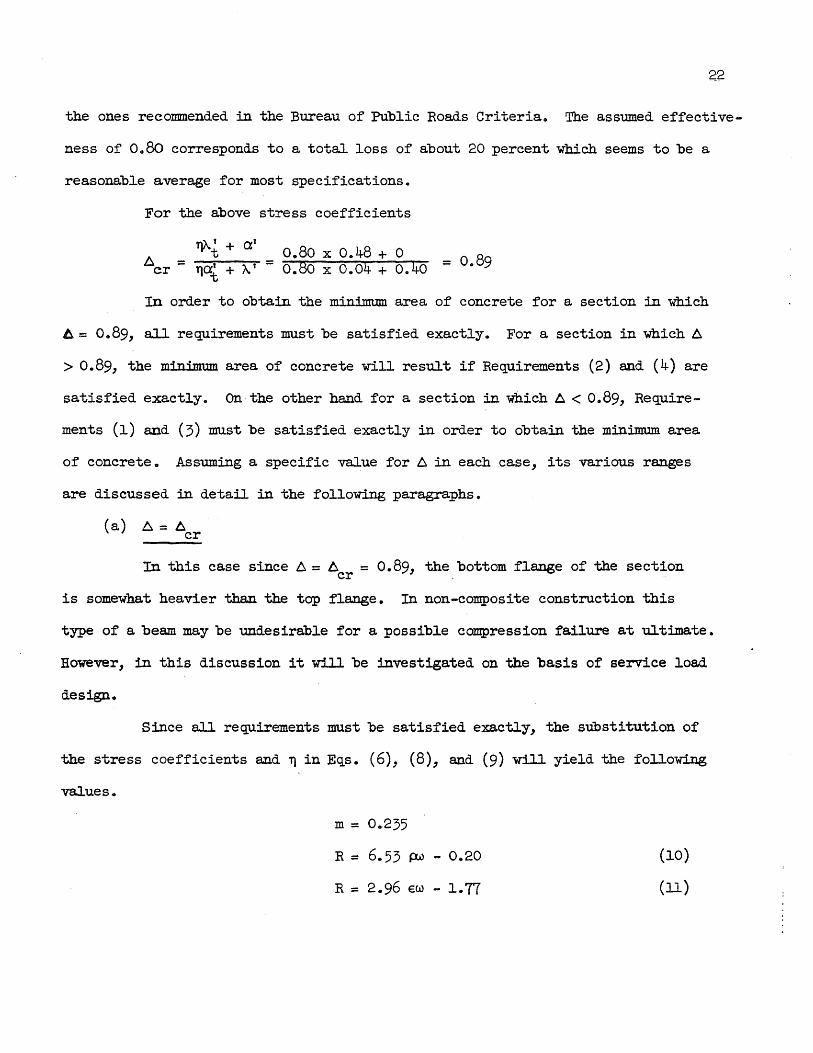
the ones recommended in the Bureau of Public Roads Criteria. The assumed effective-

ness of 0.80 corresponds to a total loss of about 20 percent whiCh seems to be a

reasonable average for most specifications.

For the above stress coefficients

TlA t + at

h. t cr = -Tl-a":""i -+-~--:-f = t,

o.Bo x 0.48 + 0 0.80 x 0.04 + 0.40 = 0.B9

In order to obtain the minimum area of concrete for a section in Which

6= 0.B9, all requirements must be satisfied exactly. For a section in which 6

> 0.B9, the minimum area of concrete will result if Requirements (2) and (4) are

satisfied exactly. On the other hand for a section in which 6 < 0.B9, Require-

ments (1) and (3) must be satisfied exactly in order to obtain the minimum area

of concrete. Assuming a specific value for h. in each case , its various ranges

are discussed in detail in the following paragraphs.

(a) ~=6 cr

In this case since 6 = 6 = 0.89, the bottom flange of the section cr .

is somewhat h~avier than the tqp flange. In non-composite construction this

type of a beam may be undesirable for a possible compression failure at ultimate.

However, in this discussion it will be investigated on the basis of service load

design.

Since all requirements must be satisfied exactly, the sUbstitution of

the stress coefficients and Tl in Eqs. (6), (B), and (9) will yield the following

values.

m = 0.235

R = 6.53 pw - 0.20

R = 2.96 €W - 1.77

(10)

(ll)

(b) b. > D. cr

This case is the most practical one; the rectangular sections, sym-

23

metrical I-sections, and all sections in which the top flange is heavier than the

bottom flange, are in this category. In this case in order to obtain the minimum

area, Requirements (2) and (4) must be satisfied exactly. In order to study the

two least weight criteria a particular value of D. such as A = 1 will be assumed.

Criterion I: It has been shown that in this case it is necessary to

satisfy Requirements (1), (2), and (4) exactly and (3) by a margin.

Wi th the exception of' A. all stress coefficients are known and A. can be

computed from Eq. (5) taking ~ = 1.

ry.... + a' A. = t~ - T} at = 0.384 - 0.032 = 0.352

Hence for D. = 1, the stress coefficients corresponding to Criterion I

will be

at = at = 0.04

A.t = A.t = 0.48

A. = 0.35

a = at = 0

Substituting the above coefficients in Eqs. (6), (8), and (9), the

following will be obtained:

m = 0.22

R = 6.14 p.d - 0.20

R = 2.60 €W - 1.68

(~Oa)

(lla)

The above equations are based on the assumption that b. is equal to unity.

Sim:ilar equations can be derived for other vaJ.ues of ~ which are greater than 0.89.

24

Table 1 contains Eqs. (lOa) and (lla) for values of 6 equal to 1.00, 1.25, 1.50,

1.75, and 2.00.

Criterion II: It can be shown that in this case Requirements (2), (3),

and (4) must be satisfied exactly and (1) by a margin.

In this case all stress coefficients are known except at which can be

computed from Eq. (5) taking ~= 10

ll"" f + a f

(t _ ~,) ~

= -0.02

Hence for ~ = 1, the stress coefficients corresponding to Criterion II

will be

at = -0.02

""t = ~' -t - 0.48

~ = A,v = 0.40

a = a' = 0

Substituting the above coefficients in Eqs. (6) and (9) the following

will result

m = 0.25

R = 3.34 €W - 1.87 (lib)

From Eq. (8a) it can be seen that for a given value of~, R is only

dependent upon tva stress coefficients ~t and o. Therefore, substitution of the

above coefficients in Eq. (6) will result in Eq. (lOa).

A tabulation of Eq. (lib) for values of ~ equal to 1.00, 1.25, l.50,

1.75 and 2.00 is also included in Table,l.

(c) D.<~ cr

This case is rather uncommon in non-composite construction. The sec-

tions corresponding to this case include inverted T-sections and sections in

25

which the bottom flange is heavier than the top flange. Beams in this category

are undesirable since they may fail in compression. However, they will be discussed

here on the basis of service load design.

In this case in order to obtain the minimum concrete area, Requirements

(1) and (3) must be satisfied exactly. To illustrate the discussion 6 wili be

assumed as 0.50.

Criterion III: It has been shown that in this case it· is necessary to

satisfy Requirements (1), (3), ·and (4) exactly and (2) by a margin.

All stress coefficients are known except At which can be computed from

Eq. (5) taking ~= 0.50.

"'t = ~(Tlat + A. I )

Tl

- at = 0.27

Hence for A= 0.50, the stress coefficients corresponding to Criterion

III will be

at = at = 0.04

A.t = 0.27

f... = At = 0.40

a = a' = 0

Substituting the above coefficients in Eqs. (6), (8), and (9), the

following will result:

m = 0.167

R = 5 .18 p.u - 0.20

R = 2.78 €W - 2.29

(lOc)

(llc)

Table 2 contains a tabulation of Eqs. (lOc) and (lic) for vaJ.ues of D.

equal to 0.50, 0.571, 0.667, and 0.80

26

Criterion IV: It can be shown that in this case it is necessary to

satisfy Requirements (1), (2), and (3) exactly and (4) by a margin.

All stress coefficients are known except a which can be computed by Eq.

(5) tak~g 6 = 0.50.

-1lAt = -0.168

Hence for 6= 0.50, the stress coefficients corresponding to Criterion

IV will be

at = at = 0.04

At = A,' -t - 0.48

A, = A,f = 0.40

ex = -0.168

Substituting the above coefficients in Eqs. (6) and (9) and simplify-

ing the following will result:

m = 0.306

R - 3.04 €W - 1.45 (lid)

A tabulation of Eq. (lid) for vaJ.ues of 6. equal· to 0.50, 0.571, 0;667,

and o. 799 and 0.89 is aJ.so included in Table 2.

The values of m and the stress coefficients for Criteria I and II are

shown in Table 3 for convenient reference. Table 4 shows a similar tabulation

for Criteria III and IV.

It can be concluded that on the basis of least weight design, for a

given value of 6, (l) the quantity m can be obtained, (2) linear relationships

between R and w can be established.

27

15. The Relationship between € and the Cover Ratio

The quantity €, which is defined as the ratio of eccentricity to the over

all depth of the beam (e/h) seems to be a convenient variable in 'this study. How-

ever, practically it is more convenient to estimate the cover ratio than €. The

cover ratio is defined as the ratio of the distance between the bottom fiber and

the center of gravity of steel to the overall depth of the beam. The cover which

is the distance of the bottom fiber to the center of gravity of steel is designated

by c in this study.

It can be shown that for any section the following expression is correct:

Table 5 shows the values of € for different vaJ.ues of ~ and three val

ues Of~, namely, 0, 0.1, and 0.2. The values of € corresponding to ~ = 0 have

no practical meaning. They are given in order to show the limiting conditions.

It should be noted that all values of E chosen in the subsequent study

are based upon the three values of ~ mentioned above.

16. The Graphical Representation of Relations among the Unknowns

In order to facilitate the study of relations among the unknows it is

desirable to plot all equations defining the relationship between R and w for the

four criteria discussed in the preceding section. In the following paragraphs

the plots are discussed for each case.

(a.)

In this case ~ = 0.89 and m = 0.235. Eqs. (10) and (11) are plotted in

Fig. 1 taking w as abscissa and R as ordinate. The ordinate is varied from zero

to 10 and the abscissa is taken from zero to 15. The range for w and R is in

28

accordance with practical sections. Equation (10) which contains the parameter p

has been plotted for four values of p namely, 0.08, 0.10, 0.12, and 0.14. The

range of p corresponds to practical sections. Equation (11) which contains the

parameter E has been plotted on the same figure with broken lines using three

values of E, 0.271, 0.371, and 0.471. The thick broken line marked € = 0.471,

corresponds to a case in which the center of gravity of the prestressing steel

is at the bottom fiber. The other broken lines for € of 0.271 and 0.371 corres

pond respectively to ~ of 0.20 and 0.10.

(b) 6>1::. cr

In this ease the variation of w with R has been plotted for Criteria

I and II assuming various values of 6.. Figure 2a shows the plot of Eqs. (lOa)

and (lla) for Criterion I when t::. = 1. As before w is taken as abscissa and

varied fram zero to 15, while R is taken as ordinate and varied between zero

and 10. Equation (lOa) has been plotted for five values of~, namely, 0.08,

0.0833, 0.10, 0.12, and 0.14. The line corresponding to p = 0.0833 is drawn as

a heavy line to show distinctly the relation between R and w for a rectangular

section. Equation (lla) has been plotted on the same figure with broken lines

for values of € equal to 0.3, 0.4, and 0.5. The plot for € = 0.5 corresponds

to a case in which the center of gravity of steel is at the bottom fiber and is

shown with a heavy broken line. Similarly the broken lines for € of 0.3 and 0.4

correspond respectively to ~ of 0.20 and 0.10.

Figure 2b shows the plots of Eqs. (lOa) and (llb) corresponding to Cri-

terion II when l:::. = 1. Evidently, Eq. (lOa) is the same in Criteria, I and II and

is plotted ~ain in Fig. 2b. ,Equation (lib) has been :plotted on the same figure

using the same values for € as in the preceding case.

29 •

Figures 3a through 6b show similar plots for Criteria I and II for four

values of 6, namely 1.25, 1.50, 17.5, and 2.00. In each case the same ordinate

and abscissa are used and similar values for p and E are taken. In each case the

plot corresponding to the limiting value of E is shown with a heavy broken line.

(c) 6<b. cr

The graphical presentation is identical with the preceding case. The

variation of w with R has been plotted for Criteria III and IV assuming various

values for~. Figure lOa shows the plots of Eqs. (lOc) and (llc) for Criterion

III When ~ = 0.50. Figure lOb shows the plots of Eqs. (lOc) and (llc) for Cri-

terion IV when for the same value of b.o The same abscissa and ordinate have been

used as before and the values of p and E are similar to the preceding case.

Figures 7a through 9b show similar plots for Criteria III and IV using

values of b. equal to 0.571, 0.667, and 0.800

17. The Interpretation of Relations among the Unknowns

Important conclusions can be drawn from the mathematical and graphical

presentation of relations between R and w for the four criteria in the preceding

sections. In the following paragraphs these conclusions are restated and sum-

marized.

In order to obtain the least area of concrete, it is necessary to satisfy

the four requirements exactly. This can be done only for a specific position of

the neutral axis, that is, b. must be equal to the known value of b. • In this cr

case b. and m have specific numerical values and the variation of R with w is de-

fined by Eqs. (10) and (11) as plotted in Fig. 1. Equation (10) defines the cross

sectional area of the beam, while Eq. (11) defines the eccentricity. For a given

depth, w is known and E can be estimated on the basis of a minimum cover. From

30

Fig. lone can conclude that an increase in p will result in an increase in R and

a decrease in the cross sectional area. The value of P, however, should be low

enough to provide a sufficient cover.

Since in most specifications 6 < 1, satisfying four conditions exactly cr

will result in beams with a heavy l)ottom flange in comparison with the top flange.

For a value of 8 other than 6cr' it would no longer be possible to satisfy the

four requirements exactly. One or more reCluirements will have to be satisfied

with a margin resulting in a heavier section.

If l::. > l::. , for the least weight section, Requirements (2) and (4) must cr

be satisfied exactly and Criteria I and II have been defined. Therefore, for a

specific value of l::. and w both criteria will produce the same cross sectional

area. In other words the variation of R with w for a given value of p is the

same in both criteria.

The variation of R with w for a given value of € is not the same in

Criteria I and II. Since Criterion I reCluires the minimum area of steel for the

area of concrete chosen, a larger value of € is needed. In Criterion II, since

the required area of steel is the maximum for the area of concrete chosen, the

value of € reCluired is smaller.

A study of Figs. 2a and 2b results in an important conclusion. For

small values of w, the efficiency is limited in Criterion I because of limita-

tions on eccentricity, while in Criterion II, since € is comparatively large, a

higher efficiency might be possible. It can be concluded, therefore, that for

small range w Criterion II might produce a lighter section. For example, assume

that 8 = 1, W = 5 and it is necessary to have € = 0.40. Applying Criterion I,

from Fig. 2a the maximum possible p will be about 0.12 corresponding to a value

of R which is about 3.5 Applying Criterion IIJ from Fig. 2b the value of P is

31

more than 0.14, resulting in a value of R that is somewhat higher than 4. It

should be emphasized, however, that there is a practical limitation on P, and in

many cases P = 0.14 may not be realized 0

The above conclusions can be generalized to sections in which ~ is

greater than unity. A study of Figso .3a through 7b will indicate that the gen-

eral characteristics of the plots are the same.

A comparison of Figs. 2a and 3a. shows that when .6 = 1, the slope of the

line relating R to w for a ~ecific value of p is greater than the corresponding

slope wen .6 = 1.25. A study of Figso 2a through 7b indicates that the greater

~ becomes in comparison with D. , the greater the area required for given w and . cr

p values.

If 6. < D. , it has been shown that for the least weight design Requirecr

ments (1) and (3) must be satisfied exactly and in this case Cri teria In and IV

have been introduced. Therefore, for a specific value of D. both criteria will

produce the same cross sectional area. In other words, the variation of R with

w for given values of P is the same in both criteria.

The variation of R with w for given values of € is not the same in

Criteria III and IV. For the same 1:::., w, and P a greater € is necessary in Cri-

terion III in comparison with Criterion IV. The general characteristic of each

plot is identical with plots already discussedo

Similarly from Figs. 7a throU&~ lIb it can be concluded that for given

P and w, the smaller D. becomes in comparison with I:::. the greater the area recr

quired.

18. Derivation of Expressions for p and I:::. for Various Types of Sections

On the basis of the discussions in the preceding sections a convenient

procedure may be developed for service load design of non-composite sections.

32

However, before a design can be made it is necessary to develop relationships among

P, 6., and the proportions of the sectiono

It can be shown that for symmetrical I-sections such as shown in Fig. 11

the following expression is correct:

l - (l - b 1 !b) (l - 2 t/hf p = 12 [1 - -( 1 - b Y/b) ( 1 - 2 t h )] (12)

in which

b = the width of the flange,

b' = the thickness of the web,

t = the thickness of the flange, and the other terms

have been defined previously.

Equation (12) is plotted in Fig. 11. The efficiency p is taken as Qr-

dinate and varied from zero to 0025; t/h is taken as abscissa and varied from zero

to 0.50. In plotting Eq. (12) b'/b is taken as 0.10, 0.20, 0.30, 0.40, and 0.50.

For a T-section such as shown in Fig. 12 the following relations can be

established:

in which

p - r2 _ 1 [t /h (1 - b. 2 ) + 2b. - 1 ] - h 2 - 3 (1 + 6)2

~ = Yb = 1 - (1 - b!!b) (1 - t/h)2

Yt 1 - (1 - bf/b) 1 - (t/h)2

b = the width of the flange

b' = the width of the stem

t = the thickness of the flange, and the other terms

have been defined previously.

(13)

(14)

33

Equations (13) and (14) are plotted in Fig. 12. Equation (13) repre-

senting the variation of p with t/h is plotted in Fig. 12a. The efficiency p is

taken as ordinate and varied between 0 0 05 and 0.12; t/h is taken as abscissa and

varied from zero to 0.50. In this plot b, is taken as 1025, 1.50, 1.75 and 2.00.

Equation (14) is plotted in Fig. 12b taking b'/b as ordinate and t/h as abscissa.

The ordinate b'/b is varied from zero to 0.70; the abscissa t/h is common with

that in Fig. 12a and the same values of b, have been used.

For an inverted T-section such as shown in Fig. 13, the following re-

lations can be established:

2 r

.p = 2= h

[ t/h (1 -~) + ~ - 1] 1 2 b,2 b.

3 ( 1 + ~)

1

bf t 2 1 - (1 - b) 1 - (h)

b' t 2 1 - (1 - b") (1 - il)

(15)

(16)

Equations (15) and (16) are plotted in Fig. 13 similar to the plots of

the T-section.

It should be pointed out that Eqso (15) and (16) can be obtained from

Eqs. (13) and (lL) respectively by substituting ~ for all values of~. Figure 13

therefore, \.loWd be identical with Figo 12 if instead of~, the reciprocal of b,

were considered. Although one set of curves is sufficient to show the relationship

among the secticn properties of T and inverted T-sections, for convenient reference

two curves are presented.

For an unsymmetrical I-section in which the thickness of top and bottom

flanges is the same and the width of the top flange is twice that of the bottom.

flange, the following expressions are correct:

34

t 2 t (-) (6 + 1) - 2 - (2 - 6) h h

t (18) 2 (2 - - 1) (~ - 1)

h

in which b is the width of the top flange and Eqso (17) and (18) are plotted in

Fig. 14.

For an unsymmetrical I-section in which the thickness of top and bottom ~

flanges is the same and the width of the bottom flange is twice that of the tqp

flange the following expressions are correct:

t 2 t (-) (6 + 1) - 2 - (~ - 1) h h

t 2 (- - 2) (1 - ~) h

Equations (19) and (20) are plotted in Fig. 150

(20)

Evidently Eqs. (19) and (20) can be obtained from Eqs. (17) and (18) re

spectively by substituting ~ for all values of ~o

The following steps may be followed in designing a beam:

1. Choose a value for ~; on the basis of the previous development it is

desirable to be as close to ~ as possibleo cr

2. Choose values for h and p. The choice of h is not a structural

problem and should be determined considering the clearance requirements and the

35

height of the building. The efficiency p can be estimated accurately if the type

of the section is known. For a symmetrical I-section p should be in the order of

O.l2 for T -beams about 0.09.

3. Compute w, R and the cross-sectional area.

4. From E~s. (12), (13), and (14), whichever applies assume a value

for t/h and determine b t lb. Since A is known, b can be computed. In completing

this step the tentative proportions of the section are determined.

5. Compute the eccentrici ty corresponding to the minimum and maximum

steel areas. If the maximum eccentricity corresponding to a sufficient cover is

within this range it can be adopted. Otherwise the assumptions of ~ h and p

should be revised.

19. Introduction

CHAPTER III

ULTIMATE FLEXURAL STRENGTH OF BEAMS

WITH BONDED REmFORCEMENT

In the preceding chapter the first group of design criteria, that is

the criteria for service loads, were investigated independently. Before study

ing the criteria in the second group, the ultimate design criteria)the ultimate

flexural theory of beams will be examined. Since the ultimate design criteria

are based on ultimate flexural strength of beams, it is necessary to understand

the theory and methods used in the determination of flexural strength.

This chapter contains a brief presentation of the general theory,

which forms the basis for estimating the ultimate moment carrying capacity of

a prestressed concrete section. In addition, a comparative study is made of

several simplified procedures, which give results fairly close to those ob

tained by using the more exact and elaborate methods. The simplifj~g assump

tions made or implied in these procedures, and their limitations, are also dis

cussed. It is not the purpose of this chapter to introduce a new theory, but

only to restate the significant ideas concerning the ultimate strength of beams

in flexure, as a.d.a.pted to accommodate this study.

20. General Expression for Ultimate Moment of a Beam

A flexural failure takes place mostly by crushing of concrete, the

corresponding tensile strain in the steel being within or outside the elastic

range, depending on whether the beam is over or under-reinforced. Failure by

fracture of the reinforcement is rare.

37

Computation of the ultimate moment in a beam with bonded reinforcement

is based on the following assumptions;

l~ Strains are distributed linearly across the section at all stages

of loading.

2. At failure, the extreme fiber strain in concrete corresponds to a

limiting value which is practically independent of the ~uality of the concrete

and which lies in the approximate range from 0.003 to 0.004.

3. The compression stress block at ultimate load is curvi-linear

with an average stress which varies from about ft to 0.8 f', for ff ranging from c c c .

3,000 to 8,000 psi. Also the resultant compression acts at a distance from the

compression face e~ual to 0.40 to 0.45 times the depth of the stress block.

4. Perfect bond is maintained between concrete and steel.

5. No tension is resisted by the concrete.

The assumption~ regarding linear distribution of strain, the limiting

strain for concrete in flexural compression and presence of perfect bond are

generally inaccurate. However, by means of these assumptions it is possible to

establish a theory which can be used with reasonable accuracy in computing the

flexural strength of bonded beams. The characteristics of the fully developed

stress block are supported by experimental evidence. The tensile resistance of

concrete is small and its contribution to the ultimate moment may be neglected.

If the values of the limiting strain, average stress, and the location

of resultant compression are known or assumed, the ultimate moment can be esti-

mated by simultaneously satisfying the re~uirements for static e~uilibrium, geo-

metric compatibility of strains and the stress~strain relation of the reinforce-

mente

For rectangular sections or for flanged sections in which the neutral

axis lies within the flange the following expression can be written from statics:

in which

pf M = A f d (1 - k_ f SU)

U S su C

M u

A s

f su

d

~

cu

= the ultimate moment

= the area of the prestressing steel

= the stress in steel at failure of the beam

= the distance from the center of gravity of steel to

the extreme compression fiber

= the ratio of the distance of the compression force

from the compression fiber to the depth of stress block

= the percentage of reinforcement taken as A /bd in w.hich s

b is the width of the compression flange

f = the average compressive stress cu

(2l)

An expression similar to Eq. (21) can be derived for flanged sections

in which the neutral axis falls below the flange. However, sections of this

type will not be discussed here, since the purpose of this section is to review

and emphasize the bases of the ultimate theory.

in which

From the assumed strain distribution we have:

pfsu -r-= €

eu su

€ U

- € - € + € se ce u

€ = the limiting strain in concrete at failure u

e = the strain in steel at failure of the beam su

(22)

Ese = the strain in steel due to the effective prestress

E = the strain in concrete at the level of steel due to ce

effective prestress

other terms have been defined.

The steel stress f can be obtained from Eq. (22) with the use of the su

pertinent stress-strain relationship. The ultimate resisting moment may then be

evaluated by substituting the value of f so found in Eq. (21). It may be ob-. . su

39

served that Eqs. (21) and (22) are general and applicable to both under and over-

reinforced beams.

The procedure outlined above for obtaining the steel stress at failure

of the beam is rather complicated. It involves either a trial and error proce-

dure or the use of arbitrary algebraic equations fi~ted to the stress-strain

curve for the steel. These procedures are hardly justifiable for routine design

and difficult to handle for purposes of analytical study. Several simplified

expressions are discussed in the subsequent sections.

21. Method Suggested by Professor C. P. Siess (4)

For under-reinforced beams, € lies in the inelastic region of the su

stress-strain curve, and it has been observed that the steel stress f at su

failure of the beam may be estimated accurately by the following empirical re-

1ation:

in "Which

f = f' - .9:... (ft - f ) s sy su s ~

f = the stress at yield, usually taken as the stress corresponding sy

q

to 0.2 percent plastic set pf

sy = a measure of percentage of reinforcement taken as f cu

~ = the value of q corresponding to balanced failure (in which

f = fsy) and is given by the relation su

E u '\, =

E - € - € + E sy se ce u

Equation (23) represents a linear relation between f and q when f varies be-su su

tween f' andf as q varies between 0 and a.. • s sy -0

Substituting for f from Eq. (23) in Eq. (21) and rearranging, we have: su

in which f

Cl = 1 - ~ and f' s

(24)

Equation (24) checks very closely with test results reported by Billet

and Appleton (3), Sozen (8), and Warwaruk (7), for under-reinforced beams. A

fairly satisfactory agreement is observed even for over-reinforced beams for

values of q as high as 1.5 ~ with an increasing degree of conservatism which

seems desirable.

Equation (24) may be further simplified by neglecting the term C1 C2

which is small.

The factors affecting the value of ~ usually vary within the follow

ing relatively narrow range.

€ = 0.003 to 0.004 u

E = 0.01 sy

Ese = 0.0033 to 0.005

E = 0.0004 ce

The corresponding value of ~ would vary between 0.32 and 0.47_

Assuming: ft = 250 ksi s

'f = 210 ksi sy

= 0.42 f

We have: -_ 1 sy 0 16 - rr- = • s

C2 = ~ ~ = 0.134 to 0.197

Thus Cl + C2 varies from about 0.294 to 0.357 with an average value

1 of' about 3 •

Equation (21) may then be rewritten as follows:

M = A f' d (1 - ! .9-..) U ss 3CJu

22. Methods Specified in the Bureau of Public Roads Criteria (5 )

The following is specified:

41

Where the prestressing elements are bonded to the concrete, reinforce-

ment sha.1.l be assumed balanced if

0.8 1" c

0.23 -f~t-s (27)

When p is equal or less than~, the ultimate moment Mu shaJ.l be de

termined as follows:

pression:

M = 0.9 Asf'd u s (28a)

Wben p is greater than ~, Mu shall be computed by the foilowing ex-

M = u 1" d s

Where ~s = steel area for a balanced section.

The above elluation may be expre"ssed in terms of ~ as follows:

Mu = O.9J~ Asf~d where p = A /bd

s

Substituting for Pb from Ell- (27)) the above equation can be expressed

as follows:

M = 0.9 u

0.8 f' c

pf' s A f'd s s

23. Method Proposed by the Joint Committee (6)

(2&)

The Joint ACI-ASCE Committee 323 Which is in charge of specifications

for prestressed concrete structures is considering several methods for comput-

42

ing the ultimate flexural strength of fully-bonded beams. None of these methods

has yet attained an official status and may not even appear in the final version

of the recommended practice. However, one of the more elaborate methods will be

discussed here for the sake of interest.

For rectangular sections or for flanged sections in which the neutral

axis lies within the flange,. the ultimate flexural strength is given by the fol-

lowing expression:

It is assumed that when the flange thickness is less than 1.2 dpf If' su c

the neutral axis will fall outside the flange and the following approximate ex-

pression for ultimate moment is given:

( Asrf su) 8 f I ) ( ) M = A f d 1 - 0.5 b 1 df ' + O. 5 c (b -b' t d-O. 5t u sr su c

where Asr = As - Asf = the steel area considered to act with the rec

tangular section of width b t•

A f = 0.85 f' (b-b') tlf = the steel area required to develop s c su

the compressive strength of the overhanging portions of the flange.

The following empirical and approximate expressions. for f are ~ecisu

fied for use in Eqs. (29a) and (29b) provided that the following conditions are

satisfied:

1. The stress-strain properties of the steel display a high yield

strength coupled with a substantial elongation before rupture. (In the pro-

posed specifications a whole section is dedicated to the required and desirable

properties of steel.)

2. The effective prestress after losses is not less than 0.5 ft. s

3. The vertical distribution of the reinforcement at the section con-

sidered does not extend more than 0.15 d above or below the centroid of steel

area considered.

pf' fsu = f~ (1 - 0.5 f,s)

c (30)

In order to avoid the use of over-reinforced beams, the percentage

of prestressing steel should be such that the ratios p f If' for rectangular su c

sections and A f Ibtd f' for flanged sections be not more than 0.30. sr su c

If a steel percentage in excess of this amount is used, the ultimate

moment shall be taken as not greater than the following values:

(a) Rectangular Sections

0.25 f' bd2 c (3la)

(b) Flanged Sections

M = 0.25 bd2

ft + 0.85 f' (b-b t )t(d-O.5t) -ll c c (3Ib)

A minimum amount of steel percentage is also specified to avoid pos-

sible failure of a beam by fracture of the prestressing steel.

In the actual proposed specifications, expressions are also included

for computing the flexural strength of the unbonded beams. In this study since

only bonded beams are considered these expressions are not included.

24. A Comparative Study of the Simplified Methods

The expression for ultimate moment used in the three methods discus-

sed may be written in the following general form:

M = A f~Kd u s s

The quantity Kd may be thought of as an equivaJ.ent internal moment

arm at failure. Actually it is not the true moment arm for it corresponds to

a tensile force A f' instead of A f • s s s su

The major variable which affects the value of K may be taken as

For a comparative study of the ultimate moments computed by the

three methods, it is sufficient to study the variation of K versus q for each

method.

It is necessary therefore, to establish a relationship between K and

q for each of the methods discussed.

The following assumptions are made:

€ = 0 .. 0034 u

€ = 0.0100 sy

44

€ = 0.0050 se

€ = 0.0004 ce

f = 0.8 f' cu c

f' = 250,000 psi s

f = 210,000 psi sy

f = 150,000 psi se

On the basis of the above assumptions, the value of ~ in the equa

tion suggested by Professor C. P. Siess is 0.425, and K can be presented as

1 q ) K = (1 - 3" ~ = 1 - 0.785 q (32)

According to the Bureau of Public Roads Criteria the value of K is

45

constant and is equal to 0.9 when p is less than ~. The expression for ~ can

be written as follows:

0.8f' c

Pr, = 0.23 f' = 0.23 s

f sv 210 84

since rr- = 250 = 0. s

pt :: 0.193 f cu f sy

f f cu sy f fI sy s

Eviient1y in the Bureau of Public Roads Criteria ~ = 0.193. The

following can be concluded:

For ~ < 0.193:

K = 0.9 (33a)

For q > 0.193: f

K 0.9 sy = 0.23 fT

q s

j )

1 )

S it

46

or K = 0.396

'{cl

Tbe proposed recommendations of the Joint Committee will be studied for

rectangular sections and sections in which the neutral axis falls below the flange.

Substituting for f from ECl. (30) in ECl. (29a) and rearranging, the following su

value of K will be obtained:.

or

since

hence

fS f f f' s sy cu s

p F = P f rr f = 0·953 Cl c cu c sy

2 K = (1 - 0.477 Cl) (l - 0.477 q + 0.226 Cl )

f

(34a)

E Clua tion (34a) is applicable on.1.y when p f ~u :s. o. 30, or Cl :s o. 37 • c

For values of Cl ~0.37 the following expression is given:

M u

A dfl S S

ft o 25 c 0.25

= K = • pf ~ = 0.953 Cl

K = 0.262 Cl

(34b)

To summarize the preceding discussion the values of K are tabulated for

each of the three methods discussed:

Method

Method by Professor

C. P. Siess

Bureau of Public

Roads Criteria

Joint Committee

Recommendations

(Rectangular Sections')

K

K = 1 - o. 785 Cl

(Cl ~ 0.64)

q :s 0.193: K = 0.9

q .2: 0.193: K = 0.396/ Cl

q :s 0.37:

q .2: 0.37:

K = (1-0.477q) (1-0.477q +

0.226 q2)

K = 0.262/q

The variation of K versus Cl is shown graphically in Fig. 16 for the

three methods discussed. The factor K is taken as ordinate and var_ied between

0.3 and 1.0 while q is taken as abscissa and varied between zero and 0.6.

To show the variation of K versus q in Professor Siess' Method, Eq.

47

(32) in which ~ = 0.425, has been plotted in Fig. 16. This line is marked (1)

in the figure. The line marked (2) corresponds to a line with a ~ of 0.378.

The variation of K versus q for the Bureau of Public Roads Criteria is

presented in the same figure by plotting Eqs. (33a) and (33b). The curve is

marked (3) in the figure.

Equations (34a) and (34b) are similarly plotted in Fig. 16 to show the

variation of K versus q for the Joint Committee recommendation. The curve is

marked (4).

To show the accuracy of ea.ch method the results of 37 beam tests are

plotted designating each beam by a point. These beams were tested at the Univer-

sity of Illinois by D. F. Billet (3), M. A. Sozen (8), and J. W. Warwaruk (7).

The characteristics of the beams tested and the properties of the mate-

rials used are listed in Tables 6 and 7. The actual values of K and q are listed

in Table 8.

A distinction is made in the points plotted in Fig. 16 according to the

value of f' , the effective prestress. A hollow triangle indicates an f in the se se

beam of less than 30 ksi. The beams with f between 100 ksi and 130 ksi are se

shown by hollow Circles, while the beams with f over 150 ksi are designated by se

:ruJ..l circles.

From Fig. 16 one may conclude that the three practical methods for com-

puting the flexural strength of prestressed concrete beams result in a reasonable

estimate of the value of K.

In this study two methods are used in computing the ultimate flexural

strength of beams: (1) Professor Siess' Method with q = 0.425, and (2) the

Bureau of Public Roads Criteria.

CHAPTER IV

INTERRELATIONSHIP BETWEEN SERVICE LOAD AND ULTIMATE

DESIGN CRITERIA

25. Introduction

49

In Chapter II, the interrelationship between the parameters affecting

the service load design was studied. In addition, criteria were established

which would result in sections with the least area. This chapter deals with the

correlation of working load design criteria and the corresponding safety factors

against ultimate failure. The minimum possible safety factors, and the condi

tions under which they would occur, are also investigated for a given set of de

sign specifications.

This study is carried out for both under-reinforced and over-reinforced

beams. However, if the beam is highly over-reinforced the methods used here may

not apply_ Generally, sections used in non-composite construction are I-sections

or sections with heavy top fl~ges which are mostly under-reinforced. On the

other hand, inverted T-sections and sections with heavy bottom flange are gen

erally over-reinforced. The methods used here are reasonably accurate for over

reinforced beams provided that the percentage of steel is not more than 50 per

cent over the balanced percentage.

26. The Live Load and Total Load Safety Factors

Of the loads which a beam is required to support during its service

life, its own weight and any superimposed dead load attached permanently to it

are known with a fair degree of accuracy, while there is considerable uncertainty

about the magnitude of the live load and impact that may act on the beam. Conse

quently, a smaJ.ler margin of safety is usually permitted in cases where the dead

50

load constitutes most of the load acting on the structure, while a higher margin

is required when the live load is predominant. To achieve this variable margin,

two requirements are often stipulated in design specifications for minimum ac-

ceptable safety factors.

1. The ultimate load carr-y-ing capacity should provide a safety factor

of one for the dead load, and a minimum safety factor for the live load and im-

pact.

2. The ultimate load carrying capacity of the beam should provide a

minimum safety factor for the total load.

Since the ultimate load carrying capacity is based on flexure, the

first requirement can be written as follows:

in which

M = the moment due to the weight of the beam g

M = the moment due to the superimposed dead load s

1\ = 'the moment due to live load and impact

Nl = the live load safety factor

In the Bureau of Public Roads Criteria a minimum value of 3 is speci-

fied for Nl •

The second requirement can be written in the foliowing form:

in which

Nt = the total load safety factor

In the Bureau of Public Roads Criteria a minimum value of 2 is speci-

f'ied for Nto

51

The above requirement for Nt ensures that an adequate overall margin of

safety is available, even for structures with high dead load to live load ratios.

The use of the specification for Nl alone in a structure with no live load would

give a total load safety factor of only one, that is, no margin of safety at all.

According to the minimum values for the live load and total load safety factors

specified in the Bureau of Public Roads Criteria, Nl or Nt would govern depending

on whether the ratio of live load to dead load is more or less than one.

It may be pOinted out here that safety factors given in specifications

are necessarily related to the precedure used for computing the ultimate strength.

It is very important to realize that safety factors determined according to ,any

particular specification are only a relative measure and by no means absolute

representations of the actual margin of safety available for a given structure.

In order to establish a relationship between Nl and Nt the two expres

sions for M are equated as follows: u

and

or

Hence

Nt =

Introducing

R' =

M +M +Nlx~ g s -j.

M +M +M.. g s -~..L

!\ - 1) + 1 M(Nl t

~ Mt

Nt = Rt (Nl - 1) + 1

52

Figure 17 shows the plot of the above relation for various values of R'.

In this plot Nt is taken as ordinate and Nl as abscissa.

It is therefore sufficient to study the variation of anyone of these

safety factors. For convenience, Nt has been selected for this study_

27. The Live Load and Dead Load Safety Factors

In many specifications it is required that the ultimate load carrying

capacity should provide minimum safety factors for dead and live loads_ Assuming

that the ultimate capacity is based on flexure, this requirement can be written

as follows:

in which

Nd is the dead load safety factor.

Since it is more convenient to study the variation Nt' the total load

safety factor, it is desirable to establish its relationship with Nd and N1 -

From the discussion in the preceding section, we know

or

since

hence

M = Nt(M + M + ~ ) u g s -"l

Equating the two expressions for M we have u

~ Nt = N (1 - -) d M

t

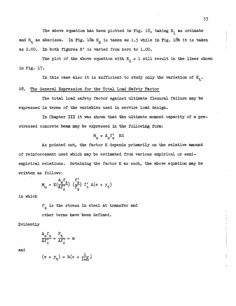
53

The above equation has been plotted in Fig. 18, taking Nl as ordinate

and Nt as abscissa. In Fig. 100 Nd is taken as 1.5 while in Fig. ISh it is taken

as 2.00. In both figures R' is varied from zero to 1.00.

The plot of the above equation with Nd = 1 will result in the lines sho~

in Fig. 17.

In this case also it is sufficient to study only the variation of Nt.

28. The General Expression for the Total Load Safety Factor

The total load safety factor against ultimate flexural failure may be

expressed in terms of the variables used in service load design.

In Chapter III it was shown that the ultimate moment capacity of a pre-

stressed concrete beam may be expressed in the following form:

M = A f' Kd u s s

As pointed out, the factor K depends primarily on the relative-amount

of reinforcement used which may be estimated from various empirical or semi-

empirical relations. Retaining the factor K as such, the above equation may be

writt~n as £ollows:

in which

Evidently

and

A f f' Mu = KCA~' s) Cr

S) f~ A(e + Yt)

c s

f is the stress in steel at transfer and s

other terms have been defined.

A f Pt s s

Aft = Af' = m c c

54

All terms in the above expressions have been defined in Chapter II.

Substi tuting the above expressions in the equation for M , the following will be u

obtained:

(35)

and by definition

or

(36)

All terms in Eq. (36) ha.ve also been defined.

From Eqs. ( 35) and (36) the total load safety fa.ctor can be computed

as follows:

M ft U (,8) ~I 1)

Nt = M = K r m r:R' € + 1 Do t s + +

From Eqs. ( 3a) and (4a) it can be shown tha. t

(MR) = p(A+a) + T)lll€

and from Eq. (6)

.b. A-a m = 11(1+6)

Substituting the above values of ~ and m in Eq. (37), we have

1 € + 1+6

(37)

Putting T}f' = f ,were f is the effective prestress, we obtain the follow-s se se

ing:

f' N = K(~) t f se

l € + l+L:l

(38) f..+a p( l+8) ty.. -Cl + €

The above exPression is general and may be used for determining the

55

total load safety factor corresponding to any given working load design criterion.

The factor K may be estimated by any of the simplified methods outlined in Chapter

III.

29. Determina.tion of Factor K

In Chapter III it was shown tha.t the most important variable affecting

the factor K is the relative steel percentage, presented by the parameter

f q = p f SY • This parameter may be expressed in terms of m u~ed in design for

cu

service loads as follows:

f A f A f f ff q - p ....2Z -...! ...9:.-~ (-EZ) (_c_) b!d - f - bd f - Af' f f

cu cu c s cu

(39)

As shown in the preceding chapter, the general expression of K accord-

ins to Professor Siess' Method is as follows:

K = (1 - 3 ~b) Substi tuting the value of q from Eq. (39) in the above equation, the

following will be obtained:

(40)

According to the Bureau of Public Roads Criteria for values of q less

than 0.l93, the factor K is a constant and is equal to 0.90. For values of q

more than 0.193 it was shown in the preceding chapter that the general expression

for K can be written as follows:

0:23 fSY q f'

s

Substituting the value of q from Eq. (39) in the above equation the

following will result:

K = 0.90 ( 41)

It should be emphasized that in this study it is assumed that the neu-

tral axis always falls in the flange.

All the quantities in Eqs. (40) and (41) are known or assumed. The

quantity !d is a shape factor and it can be shown that for rectangular sections

for symmetrical I-sections

A 1 bd = 1

€+2

and for T-sections and inverted T-sections

A 1 bd = 1

€ + l+~

(42)

(43)

(44)

It should be noted that the left side of Eq. (44) for inverted T

sections should be !rd instead of ~d •

From the above discussion it can be concluded that K is a function of

f f' f ff ...EZ c s c A, €, P, and m for given values of ~J f and f' or F and f

s cu s cu

57

A The values of bd from Eqs. (43) and (44) are tabulated in Tables 9 and

10. For convenience in Table (10) instead of E the values of ~ are listed. The

c values of E for various h ratios are listed in Table 5.

30. Variables Affecting the Total Load Safety Factor

From Eqs. (38), (40), and (41), it may be observed that the variables

which determine the value of Nt can be grouped into two categories.

The shape factors of the section constitute the variables in the first

category and are represented by 6, P, and the eccentricity ratio E. The latter

has been included among the shape factors because it defines the relative loca-

tion of the steel which is part of the "make-up" of the section.

The variables in the second category are the final stress coefficients

for concrete and steel under service loads. These are represented by ~ and a f se for the concrete and ~ for the prestressing steel.

s

The factor K as has been shown, depends entirely on the shap.e fa.ctors

and stress-coefficients included in the above groups. It can be shown that the

value of m in the expressions for K is a function of 6 and the final stress co-

efficients.

It may thus be stated that for all practical purposes, the total load

safety factor depends only on the shape of the section, as defined by the dimen-

sionless factors 6, P,

stress-coefficients ~,

and E, and the final working stresses, as defined by the

f' se ex, and rr-. The quantitative effects of variation in the s

shape factors and allowable stress coefficients on the safety factor, are dis-

cussed in the subsequent sections.

31. The Cases Investigated in this Study

By means of E~s. (38), (40), or (41) it is possible to study the varia-

tion of Nt' the total load safety factor, for various values of 6, P, € and the

stress coefficients for allowable stresses at service loads.

In order to establish a definite relationship between the design cri-

teria at service loads and the total load safety factor, the variation of the

total load safety factor for the least weight criteria will be discussed.

(a) The Least Weight Design Criteria

In Chapter II it was established that for given values of ~ >6 , cr

P, and w, the following criteria result in the least area of concrete:

Criterion I; which requires the exact satisfaction of Requirements (1),

(2), and (4) corresponding to transfer tension, transfer compression, and final

tension respectively. The corresponding area of steel is a minimum, while the

eccentricity is a maximum.

Criterion II, which requires the exact satisfaction of Requirements

(2), (3), and (4) corresponding to transfer compression, final compression, and

final tension respectively. The corresponding area of steel is a maximum and

the eccentricity a minimum.

Similarly for given values of 8 < 6 J P, and w, the following criteria cr

result in the least area of concrete.

Criterion III, which requires the exact satisfaction of Requirements

(1), (3), and (4) corresponding to transfer tension, final compression and final

tension respectively. The corresponding area of steel is a minimum while the ec-

centricity is a maximum.

Criterion IV, which requires the exact satisfaction of Requirements (1),

(2), and (3) corresponding to transfer tension, transfer compression and final

59

compression respectively. The" corresponding area of steel is a maximum and the

eccentricity a minimum.

In computing the safety factors the following ass~tions have been made

regarding the allowable stresses, average characteristics of the materials, and

the range of the section properties.

(b) Allowable Stresses:

concrete:

steel:

a' t = 0.04

Ao' t = 0.48

Ao' = 0.40

a' = 0

f se 6 rr- = o. 0 s

f se 8 1")= f= 0.0 s

The above specifications are typical and are the same as those used in

Chapter II in connection with service load design.

(c) Properties of Materials:

Concrete:

Steel:

€ = 0.0034 u

€ = 0.0004 ce

fcu 0.80 fI=

c

k2 = 0.42

f' = 250 ksi s

60

f = 210 ksi sy

€ sy = 0.01

€ = 0.005 se

E = ,3 x 104 ksi s

where:

€ = steel strain corresponding to sy

the stress f sy

E = Young's modulus of elasticity s

for steel

The above are average values for concrete and steel used in prestressed

concrete construction.

(d) Types of Sections Considered:

Symmetrical I-8ections, in which due to symmetry, l:::. = 1. The values of

p considered are 0.0833, 0.09, 0.10, O.ll, 0.12, 0.13, 0.14, and 0.15. The lowest

value of p = .0833, corresponds to a rectangular section which is a limiting shape

for the symmetrical I-section.

T-Sections, in which four values for 6 have been used, namely 1.25, 1.50,

1.75 and 2.00. Values of p considered are 0.08, 0.09, and 0.10.

Inverted T-Sections, in which ~ = 0.80, 0.67, 0.57, and 0.50 have been

used. These ar€ the' reciprocals of the 6 v~lues used in T-sections. Values of p

considered are 0.08, 0.09, and 0.10.

The above values of D. and p cover the entire range for sections with

practical proportions.

The eccentricity ratios € have been so chosen as to give cover ratios

c h equal to zero, 0.10, and 0.20.

61

32. Computation of the Total Load Safety Factors for the Least Weight Criteria

The total load safety factors have been computed using the method sug-

gested by Professor Siess and the Bureau of Public Roads Criteria.

and

On the basis of the assumptions made in the preceding section, we have

'lb == 0.425

:f sy 210 84 :r- == 250 = o. s

f f -EZ 80 sil f = o. O.60f' ==

s s

ff C f == 1.25 cu

ff

fS == 1.67 se

1.12

f f' A A q, == m f sy f c bd == 1.4 m bd

s cu

According to Professor Siess' Method

A K == 1 - 0.785q, == 1 - 1.1 m bd

and according to the Bureau of Public Roads Criteria, when q, ~ 0.193

or

K == 0.9

K == 0.334 VmA/bd

f sy 0.395

fi= s q,

• lY--- a Takmg m = T}(1+6) and 11 = 0.8, Eq. (38) for Professor Siess' Method will result

in the following:

6 A (DA-a) Nt = 1. 7 - 2.29 bd (1+6)

and for the Bureau of Public Roads Criteria

1

N = 0.498 .11+6 bd t V ~-a X-

€ + 1+6

1 € + 1+6

( 46)

62

Values of m, ~, and a corresponding to the least weight design criteria

are shown in Tables 3 and 4. The values of !d are listed for rectangular and 1-

sections in Table 9 and those for T- and inverted T-sections in Table 10.

Th al f b t d f h "t" dAd e v ue 0 q can . e compu e or eac cr~ er~on once m an bd are e-

termined. The values of K and Nt' the total load safety factor can be computed

for each method discussed above o

Tables 11 and 12 show the values of <1, K, and Nt for rectangular and

I-sections corresponding to Criteria I and 110 To make a distinction between the

two methods, the K and Nt values obtained according to the Bureau of Public Roads

Criteria are shown in parentheses.

Tables 13 and 14 contain the values of <1, K, and Nt for T-sections cor

responding to Criteria I and II respectively. Tables 15 and 16 give the same

values for inverted T-sections for Criteria III and IVo In Table 16 the values

of K and Nt corresponding to q ~ ~ are not recorded because the methods used

in this study do not apply to highly over-reinforced sections~

From Table 11 through 16 it may be observed that for given values of

6, P, and € (or ~) the use of Cri teria II and III resul ts in total load safety

factors which are always smaller ,than those given by Criteria I and IV. In fact,

in a subsequent section it will be shown that the safety factors obtained by

Criteria II and III are the smallest possible values obtainable for a given set

of allowable stress coefficients at service loads. The discrepancy in the case of

~ = 0.5 is due to the fact that the section is over-reinforced to such an extent

that the relations used for estimating K no longer apply.

It is also of interest to note that the total load safety factors~ cor-

responding to the least-weight design criteria~ lie in a relatively narrow range

(about 1.8 to 2.2 for the specifications used) in spite of considerable variation

in the shape of the section. This relative insensitivity arises from the fact

that any increase in ~ and p~ or decrease in~, tends to increase the factor K

in E~. (38)~ but has an opposite effect on the rest of the expression. The ex-

tent of this compensation would depend on the values of the shape factors them-

selves, the corresponding stress coefficients, and to some extent, on the assumed

relation between q and K. For the range of variables considered, the effect of

variation of p and ~ on Nt is not appreciable. However, any increase in the

cover ratio results in a consistent increase in Nt-

33. Criteria Resulting in the Minimum Safety Factor

It was shown in Section 30 that for given values of the shape factors

~, P, and €, the t~tal load safety factor Nt depends only on the final stress f

coefficients f.., a, and f7e • The relation given by Eq. (38) is as follows: s

€ + l+~ 1 ] -p-( l-+-~-)~~-·~-a-+-€

For values of a not more than zero, it may be shown that the term ~~a increases

with an increase in A or a. Thus the part of the expression for Nt within the

f se brackets is a min:ilnum when A, 0, and ~ are maximum.

s

64

Moreover, the factor K is a function of the parameter q, Which in turn

depends on m and f as well as the shape of the section and the characteristics of s

the materials. The relation between q and m is given by Eqo (33) and may be written

in the following form:

f' f .f' A s sy c

q=m. f • 1') • f f o bd se cu cu

or

· ~dJ &-0-f' [~ . f f'

6 sy c (47) q= 1')(1+~) · f rr-- or-se s cu

From Eq. (47) it may be seen that any increase in A. results in an increase in q,

f se while any increase in 0 or ~ tends to decrease the q value. Since the factor s

K decreases with q, it can be concluded that K decreases with A. and increases with

f se 0; or f'

s f se The overall effects of variations in A.~ 0, and ~ on Nt are as follows:

(a)

(b)

s Any increase in A. always causes a decrease in NLo

v

Any increase in a causes an increase in K and a reduction in the

rest of the expression for Nto For the range of the variables considered and the

methods used for estimating K~ the increase in K is considerably less than the

decrease of the rest of the expression for Nt- This is subject, however, to the

restriction that the beams are not over~reinforced to a degree great~r than that

corresponding to q = about 1 .. 5 ~. For higher values of q, the sim;plified methods

used result in considerable underestimation of Ks which ma.y entirely reverse the

trend indicated above.

(c) f se Increasing rr- causes a similar compensatory variation but the over-

s

all effect is generally a decrease in the safety factoro

Within the above limitations, therefore, it may be stated that for a

given set of shape factors (including €) and allowable stress-coefficients, the

lowest total load safety factor would be obtained when Requirement (3), for final

compression~ and Requirement (4) for final tension, are satsified exactly, and the

maximum permissible prestress is used. It may again be emphasized that this state-

ment is true only when at is not much more than zero or when no appreciable per-

manent tension is allowed in the concrete. For large positive values of a, the

safety factor obtained from Eq. (38) could fall below unity, if a sufficiently

small value of A is used. This apparent fallacy arises from the inconsistency of

taking account of tension in concrete at service loads and neglecting it at ulti-

mate.

For given values of ~ and p the least weight Criteria II and III--wherein

Requirements (2), (3), (4), and (1), (3), (4), respectively are satisfied--would

thus result in the lowest possible values of Nt.

From Tables 11 through 16 it may be seen that for practical sections and

for allowable stresses commonly used the minimum values of the total load safety

factor lies between 1.8 'and 2.1.

34. A Graphical Study of Variation of the Total Load Safety Factor

The conclusions drawn on the basis of the preceding discussion can also

be shown graphically similar to the study made for service load design.

ft A Substituting Eqo (7) in Eqo (38) and taking.K fS = 1.67 - 1.83 m bd

se the following will result:

(48)

where for a rectangular section

A 1 1 bd = 1 = [i2 (~ ~t) + ~ ] 1

€ + 2" + -+ m

for a symmetrical I-section

1 -12p - 1

2 12p - (1 - 2 t/h)

1 l 1 . 1 (at + ~t) + &J J iIi;- 2"

for a T-section and inverted T-section

(1 _ b.)2 1 +

. ( )2 2 3p b. + 1 - t:;.

1 l+b.

1 2"

A study of Eq. (48) and the expressions for !d indicates that for a

given least weight criterion and values of b. and P, Nt can be presented as a

function of w in the following form

in which u J v, and ware numbers which can be computed for given values of b., P

and a least weight design criterion.

66

Table 17 shows the values of u, v, and w for Criteria I and II corres

ponding to rectangular sections, symmetrical I-sections and T-sections. Table 18

similarly shows the values of u, v, and w for Criteria III and IV corresponding

to inverted T-sections.

Figures 19 through 29b show the variation of Nt versus w for various

values of p and 6. In every case w is taken as abscissa and Nt as ordinate. For

rectangular sections p has a constant value and is equal to 0.0833 and 6 = 1.

Figures 20a and 2Gb show the variation of Nt with w for rectangular sections

67

corresponding to Criteria I and II respectively_ The various values of € are shown

on ea~h curve to specify the practical range. The point shown with a solid circle

corresponds to E = 0.5 or the hypothetical condition at which the center of gravity

of steel is at the extreme bottom fiber. The hollow circles correspond to E = 0.4

and E = 0.3.

The relationship between Nt and w for symmetrical I-sections is shown in

Figs. 21a and 21b for Criteria I and II, respectively. In each case the curves

are drawn for two values of P, namely; 0.09 and 0.15. The points corresponding to

E = 0.5, 0.4 and 0.3 are shown on each curve.

Figures 22a through 25b show similar relationships between Nt and w for

T-sections. The curves are plotted for ~ = 1.25, 1.5, 1.75, and 2.0. In each

case p is taken as 0.08 and 0.10.

Figures 26a through 29b show the variation of Nt with w for inverted T

sections. Four values of 6 are considered, namely 0.80, 0.67, 0.57, and 0.5, and

curves are plotted for p = 0.08 and 0.10. Figure 19 also corresponds to inverted

T-sections in which ~ = 0.89 and all requirements are I satisfied exactly.

A study of Eq. (49) and Figs. 19 through 29 indicates that the minimum fs

safety factor possible is always greater than fiI= 1.67. The curve for p = 0.08 se

in Fig. 29b is the only exception to this rule. In this case, however, since

6 = 0.5~ the beam is highly over-reinforced and the methods used in this study

greatly underestimate the value of K.

From E~. (49) or Figs. 19 through 29 the total load safety factor of a

beam may be checked conveniently. Thus a sixth section might be added to the de-

sign procedure given in Section 21, to the effect that the total load safety factor

should be checked. If the total load safety factor is less than ,the specified

amount, the design should be modified.

68

35. Effect of Varying the Stress-Coefficients on the Total Load Safety Factor

In Section 33 it was generally stated that in the case of under-rein-

forced or moderately over-reinforced beams, any increase in the final stress co

f efficients r..., a, and f ~e , tends to increase the total load safety factor. A quan

s

titative study of this variation is presented here for the following typical sec-

tions:

(1) Rectangular Section: 6. = 1, P = 0.0833 and € = 0.40, corresponding

c toh=O.lO

(2) Symmetrical I-Section: 6.= 1, P = 0.12 and € = 0.40, which cor-

c responds to h = 0.10

T-Section: 6. = 1.50,

0.10

P ,= 0.09 and € c

= 0.50, corresponding to h =

(4) Inverted T-Section: 6. = 0.80, P= 0.09 and € = 0.344 corresponding

c to h = 0.10.

The final stress coefficients have been varied through a wide range, as

shown below:

A = 0.50, 0.40, 0.30 and 0.20

a = 0.05, 0, -0.05 and -0.10

f se f' =

s 0.60, 0.50 and 0.40

Other assumptions regarding the characteristics of prestressing steel

and concrete are the same as those used in Section 31.

The corresponding values of the total load safety factor Nt are shown in

Table 19. The values of K used are based on Professor Siess' Method for computing

the ultimate moment.

These safety factors may be considered in either of the following ways:

(a) As the lowest safety factors corresponding to any general service

f load design in which~, a and f~e are the final stress coefficients withour refer

s

ence to any specification for maximum allowable stresses.

(b) As the lowest limit of the safety factors that may result if the

corresponding stress coefficients a.re considered as the maximum allowable values.

It may also be observed that for a given type of section there is a COll-

sistent increase in

efficients ~, a and

the total load safety factor Nt when either of the stress

f ~7e is reduced. This trend is not as much pronounced for ~ s

co-

positive values of a in combination with lower values of ~, and for over-reinforced

sections. This sUbstantiates the necessity of placing certain limitations on the

values of a and ~ when a generalized statement is made. The actual limits would ~

depend on the method used for estimating the ultimate moment and also to a minor

extent on the range of shape factors considered.

The values of the total load safety factors shown are conservative and

the degree of conservatism increases rapidly as the section becomes more and more

over-reinforced. At a value of ~ in the vicinity of about 1.5, Nt is underesti-~

mated by 10 to 15 percent and for higher values no reliable conclusion can be

drawn regarding the variation. In Table 19 for values of Nt corresponding to

q > 1.5 ~ no values are recorded.

70

CHAPTER V

CONCLUSIONS

A summary of the conclusions drawn in Chapters II through IV is pre-

sented here. To save space, letter symbols and other notations which have been

defined previously are used without further explanation.

36. Service Load Design Criteria for Least Weight

(l) For given values of the depth factor w and efficiency P, a section

with the least area of concrete would result, if all four re~uirements were satis-

fied exactly. This, however, is possible only for a specific value of ~ = ~ , cr

and hence cannot always be done.

(2) For values of ~ other than 6 , the least area of concrete is obcr

tained under the following conditions:

For b. > b. , when Re~uirements (2) and (4) corresponding to the transcr

fer compression and final tension respectively are satisfied exactly.

For 6 < b. , when Re~uirements (1) and (3) corresponding to the transcr

fer tension and final compression respectively are satisfied exactly.

(3) The prestressing force (or area of steel) corresponding to the

least area of concrete is a minimum or a maximum depending on whether the remain-

ing tension or compression re~uirement respectively is satsified exactly.

(4) For given values of w and P, the four criteria discussed above re-

sult in the least area of concrete and also give the upper and lower limits of

the corresponding prestressing force and the eccentricity.

(5) For a given w and ~ the area of the section decreases with an in-

crease in P, while for given w and p it increases with an increase in 6. The

71

minimum cover requirement generally imposes a limitation on P, that is, the higher

P becomes the greater is the corresponding value of E.

37. Simplified Expressions for Ultimate Moment

(l) The ultimate flexural capacity of a section may be expressed in the

general form M = Aft Kd, where Kd may be thought of as an f1 equi valenttt internal u s s

moment arm at failure. Several approximate methods are available for estimating

the factor K. For most practical cases K varies between 0.6 and 0.9.

(2) For the practical range of variables involved, the empirical ex-

pression K = (l - ~ ~), suggested-by Professor Siess, gives results that check

closely with experimental results. It may be used for moderately over-reinforced

beams (q > 1.5 ~) with an error on the safe side not exceeding about 15%. The

expression for K according to the Bureau of Public Roads Criteria when the beam is

over-reinforced, also results in a conservative estimate of ultimate moment.

38. The Total Load Safety Factor and its Relationship with the Stress Coefficients and Section Properties

(1) It is sufficient to study only the variation of the total load safety

factor with the stress coefficients and section properties. The live load safety

factor can be obtained from the total load safety factor for a given value of the

live load to total load moment ratio.

(2) :ne total load safety factor can be expressed in terms of the final

f se stress coeffic :'ents f. and a for concrete and fT""" for the prestressing steel in ad-s

dition to the section properties.

(3) For under-reinforced and moderately over-reinforced beams, where no

appreciable permanent tension is allowed in the concrete, the total load safety

factor Nt decreases with any increase in the final concrete and steel stresses and

vice versa o

72

(4) For a given set of allowable stresses, Nt is a ~inimum when Re~uire

ments (3) and (4) are satisfied exactly. Thus Criteria II and III result not only

in the least weight but also the lowest safety factor.

(5) The effect of variation in the section properties on Nt is not very

appreciable.

(6) Any increase in the eccentricity ratio E causes an ,increase in Nt.

39. Typical Values of Nt for Sections Designed on the Bases Least Weight Criteria

(1) Values of the total load safety factor corresponding to the four

least-weight design criteria, based on commonly usea allowable stresses in concrete

and steel, lie in the relatively narrow range of about 1.8 to 2.2. Safety factors

corresponding to Criteria II and III, which are in the range 1.8 to 2.0, are also

the lowest that can result for the allowable stresses used.

(2) Sections designed on the basis of Criteria II and IV have higher

values of q and hence are more liable to be over-reinforced than those based on

Criteria I and III.

(3) For the allowable stresses used, symmetrical I-sections and T-

sections with 6 > 1 are in general under-reinforced or in some cases only slightly ~

over-reinforced. On the other hand almost all sections with 6 < 1 are over-rein-

forced. Sections with low values of p have a greater tendency to be over-reinforced.

f (4) Any increase in ~ and decrease in a and f~e cause an increase in q

s

and reduce the ductility of the beam at ultimate load.

73

REFERENCES

1.. F. R. Khan, N. Khachaturian, and C. P. Siess: "Analytical Studies of Relations among Various Design Criteria for Prestressed Concrete Beams tl

• Structural Research Series No. 105, University of Illinois, October 1955.

20 J. S.. Alagia and N. Khachaturian: tt Analytical Studies of the Relations Among Various Design Criteria for Prestressed Concrete Beams". Progress Report on Part of the Project on Investigation of Prestressed Concrete for Highway Bridges, University of Illinois, February 1956.

3. D. F. Billet and J. H. Appleton: "Flexural Strength of Prestressed Concrete Beams". Journal of the American Concrete Institute, Vol. 25, No. 10, June 1954, pp. 837-854.

4. C. P. Siess: TtStrength of Reinforced Concrete Members". Paper No.3, presented at the Symposium on the Strength of Concrete Structures, Cement and Concrete Association, London, 1956.

5" Bureau of Public Roads: "Criteria for Prestressed Concrete Bridges ft• U. S.

Government Printing Office, Washington, December 1954.

6. ACI-ASCE Joint Committee 323: "Recommended Practice for Prestressed Concrete ll,

a Report submitted to. ACI-ASCE Committee 323 for balloting. February 1957. Also proposed tfAlternate Bft Method for Computing the Ultimate Flexural Strength of Prestressed Concrete Beams, July 1957.

7 • J. W. Warwaruk: II Strength in Flexure of Bonded and Unbonded Prestressed Concrete Beams". Structural Research Series No.138, University of Illinois, August 1957.

8. Me A. Sozen: "Strength in Shear of Prestressed Concrete Beams Without Web Reinforcement fl

• Structural Research Series No. 139, University of Illinois, August 1957.

l:::.

1.00

1.25

1.50

1.75

2.00

TABLE 1. THE RELATIONSHIP AMONG R, w, P, AND E

WHEN £::. > l:::. FOR CRITERIA I AND II cr

The Variation The Variation R with w and E

74

of R with W and P Criterion I Criterion II

R = 6.144 pu - 0.20

= 5.528 pw - 0.20

= 5.120 pw - 0020

= 4.820 pw - 0.20

= 4.608 p.u - 0.20

R = 20598 EW - 1.676

= 2.030 EW - 1.528

= 10653 EW - 1.430

= 10381 EW - 1.359

= 1.180 €W - 1.307

When £::. = £::. = 0.89 cr

m = 00235

R = 6.53 pw - 0.20

R = 2.96 €W - 1.77

Specifications:

at = 0004

A' -t - 0048

A.t = 0040

at = 0

T} = 0.80

R= 3.338 EW - 1.869

= 4.219 €W -. 2.090

= 5.120 EW - 2.333

= 6.047 €W - 2.574

= 6.981 EW - 2.818

~

0.50

0.57

0.67

0.80

TABLE 2. TEE RELATIONSHIP AMONG R, w, P, AND. € WHEN

~ < ~ FOR CRrrERIA III AND IV cr

The Variation The Variation R with W and €

of R with w and p Criterion III Criterion IV

R = 5.180 j:XJ) - 0.20

= 5.452 pw - 0.20

= 5.760 pw - 0.20

= 6.221 p.u - 0.20

R = 2.780 €W - 2.29

= 2.855 €W - 2.15

= 2.880 €W - 2.00

= 2.928 EW - 1.85

When ~ = ~ = 0.89 cr

m = 0.235

R = 6.53 pw - 0.20

R = 2.96 EW - 1.77

Specifications:

a' -t - 0.04

A.' -t - 0.48

A.' = 0.40

a' = 0

T} = 0.80

R= 5.040 €W - 1.450

= 5.040 €W - 1.508

= 5.010 EW - 1.584

= 2.928 EW - 1.691

75

m

1.00 0.220

1.25 0.191

1.50 0.168

1.75 0.149

2.00 0.133

TABLE 3. VALUES OF m AND STRESS COEFFICIENTS

FOR CRITERIA I AND II I

Criterion I Criteria II at

0.040

0.040

0.040

0.040

0.040

At A ex m at

0.480 0.352 0 0.250 -0.020

0.480 0.275 0 0.278 -0.ll6

0.480 0.222 0 0.300 -0.180

0.480 0.187 0 0.318 -0.226

0.480 0.160 0 0.333 -0.260

When b. = 6 = 0.89, m = 0.235 cr

Specifications:

at = 0.04

At, = 0.48

A f = 0.40

a f = 0

11 = 0.80

At

0.480

0.480

0.480

0.480

0.480

A a

0.400 0

0.400 0

0.400 0

0.400 0

0.400 0

6. m

0.800 0.222

0.667 0.200

0.571 0.181

0.500 0.167

TABLE 4. VALUES OF m AND STRESS COEFFICIENTS

FOR CRITERIA III AND IV

Criterion III . Criterion IV at

0.040

0.040

0.040

0.040

At A a m at

0.432 0.400 0 0.249 0.040

0.360 0.400 0 0.272 0.040

0.309 0.400 0 0.291 0.040

0.270 0.400 0 0.307 0.040

When 6. = D. = 0.89, m = 0.235 cr

Specifications:

at = 0.04

At = 0.48

A.' = 0.40

at = 0

T} = 0.80

"'t A

0.480 0.400

0.480 0.400

0.480 0.400

0.480 0.400

77

a

-0.038

-0.096

-0.137

-0.168

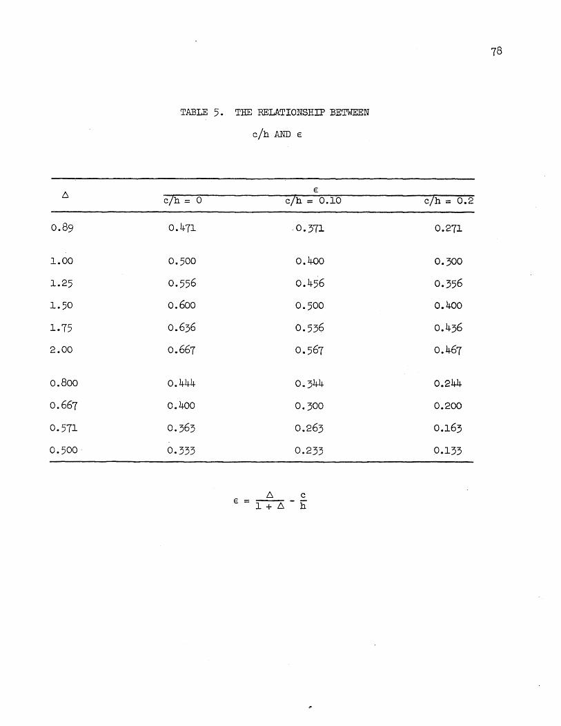
0.89

1.00

1.25

1.50

1.75

2.00

0.800

0.667

0.571

0.500 .

TABLE 5. THE RELATIONSHIP BETWEEN

c/h AND €

€

c7h = 0 c7h = 0.10

0.471 .0.371

0.500 0.400

0.556 0.456

0.600 0.500

0.636 0.536

0.667 0.567

0.444 0.344

0.400 0.300

0.363 0.263

0.333 0.233

78

c7h = 0.2

0.271

0.300

0.356

0.400

0.436

0.467

0.244

0.200

0.163

0.133

TABLE 60 THE CHARACTERISTICS OF THE BEAMS TESTED.

BY BILLET AND APPLNrON3

Beam Concrete Factor klk3 f~ Reinforce- Ultimate 0.2% Offset Effective Strength klk3 = f ment Strength Stress Prestress

ft cu p fl f f c s sy se psi psi % ksi ksi ksi

B-2 5420 0.670 3631 0.198 245.6 206.0 116.8 B-4 3440 0.413 245.6 206.0 113.9 B-5 5650 0.822 4644 0.437 249.0 219.8 114.1 B-6 2950 1.030 3039 0.695 249.0 219.8 116.0 B-7 5910 0.806 4763 0.942 249.0 219.8 112.8 B-8 3280 10130 3706 0.953 249.0 219.8 112.9

B-9 6330 0.804 5089 0.418 240.0 206.7 19.1 B-I0 3530 0.902 3184 0.107 240.0 206.7 19.0 B-l1 3910 0.979 3828 0.419 240.0 206.7 20.4 B-12 5550 0.867 4812 0.870 240.0 206.7 20.4 B-13 3750 1.040 3900 0.656 240.0 206.7 21.2 B-14 3755 1.030 3868 0.916 240.0 206.7 20.2 B-15 5710 0.703 4014 0.418 240.0 206.7 150.0 B-16 3330 1.170 3896 0.108 240.0 206.7 150.3 B-17 4580 0.745 3412 0.429 240.0 206.7 150.0 B-18 4100 0.824 3378 0.647 240.0 206.7 148.8 B-19 6225 0.778 4843 0.873 240.0 206.7 151.3

B-20 3820 0.814 3109 0.278 249.0 219.8 118.6 B-21 6560 0.744 4881 0.284 249.0 219.8 118.0 B-22 7630 0.789 6020 0.561 249.0 219.8 115.2 B-23 8200 0.716 5871 0.943 249.0 219.8 117.3 B-24 6115 0.882 5393 0.746 249.0 219.8 116.4 B-25 3270 1.000 3270 0.641 249.0 219.8 114.5 B-26 1270 1.530 1943 0.440 249.0 219.8 116.5 B-26 4590 0.842 3865 0.920 249.0 219.8 118.0

Effective Area of Depth Steel

d A s in. sq. in.

9.53 0.116 9.19 0.232 9.33 0.249 8.12 0.342 8.09 0.467 7.99 0.467

9.23 0.234 9.01 0.059 9.21 0.234 8.33 0.439 8.15 0.322 7.99 0.439 9.29 0.234 9.00 0.059 9.09 0.234 8.29 0.322 8.27 0.439

9.27 0.156 9.05 0.156 9.13 0.311 8.20 0.467 8.24 0.373 8.01 0.311 9.27 0.249 8.36 0.467

Measured Ult. Moment

M u k - in.

263 400 492 451 646 594 422 118 418 549 425 470 428 125 406 462 633 281 304 592 708 593 444 345 621

-J \0

Beam Concrete Factor Strength k1k3

f' c psi

A~12Q48 4840 00750 AQ12.60 3350 0.799 Ao22 .. 26 3665 0.760 A.32.08 )+180 0.580 A.32.11 4410 10003 A.32.17 3810 1.456

B.l1,,07 8260 0.906 B.12007 8400 0.623 Bo13,,07 8560 0.732

J-3 5280 00657 J-1 3970 0.645 J-7 5230 0.685

TABLE 7. THE CHARACTERISTICS OF THE BEAMS TESTED

BY SOZEN8

AND WARWARUK 7

k1k3 f~ Reinforce- Ultimate 0.2% Offset Effective ment Strength Stress Prestress

= f P f' f f cu s sy se psi % ·ksi ksi ksi

3630 OQ774 240 208.0 140.0 2680 00665 240 208.0 136.0 2780 0.316 240 208 .. 0 50.0 2420 0.104 240 208.0 0 41~30 00161 240 208.0 0 5550 0.218 240 208.0 0

7500 0.180 255 213.5 121.6 5230 0.181 255 213.5 125.0 6270 0.184 255 213.5 127.0

3470 0.166 267 220.0 118.2 2560 0.369 267 220.0 114.0 3580 0.658 267 220.0 112.0

Notes: (1) Beams A.12.48 through B.13.07 were tested by M. A. Sozen 8

(2) Beams J -3 through J -7 were tested by J. W. Warwaruk 7

Effective Depth

d

in.

8.20 8.81 9.28 9.24 8. 9!~ 8.85

11.07 11.05 11 .. 03

9.10 9.06 9.08

(3) Beams B.l1.07 through J-7 were I-sections with a web thickness of approximately 3 in.

Area of Measured Steel U1t. Moment A M s u

sq. in. k - in.

0.381 547 0.352 494 0.176 321 0.058 123 0.087 173 0.116 214

0.121 341 0.121 334 0.121 334

0.091 198 0.211 361 0.362 569

g>

81

TABLE 8. THE ACTUAL VALUES OF K AND Cl

M Pfsy Beam K -u = A f'd q= -f-

s s eu

B-2 0.967 0.112 B-3 0.993 0.348 B-5 0.851 0.207 B-6 0.652 0.503 B-7 0.686 0.435 B-8 0.640 0.435

B-9 0.815 0.170 B-10 0.924 0.069 B-ll 0.808 0.226 B-12 0.626 0.373 B-13 0.675 0.348 B-14 0.558 0.489 B-15 0.820 0.215 B-16 0.982 0.057 B-17 0.796 0.260 B-18 0.721 0.396 B-19 0.727 0.373 B-20 0.780 0.197 B-2l 0.866 0.112 B-22 0.838 0.205 B-23 0.742 0.353 B-24 0.774 0.304 B-25 0.716 0.430 B-26 0.600 0.498 B-27 0.639 0.523 A.12.48 0.730 0.433 A.12.60 0.664 0.516 A.22.26 0.819 0.236 A.32.08 0.956 0.089 Ao32.11 0.927 0.076 A.32.17 0.869 0.082

B.1l.07 1.000 0.051 B.12.07 0·981 0.074 B.13.07 0.982 0.063

J-3 0.895 0.105 J-l 0.708 0.317 J-7 0.648 0.404

82

TABLE 9. V ALVES OF A/bd FOR I -SECTIONS

.p t/h ALbd, € = 0050 € = 0.40 € = 0.30

0.0833* 10000 1.111 1.250

0.10 00818 0.909 1.023 0.09 0.20 00889 0.988 1.ll1

0.30 00913 1.014 1.141 0.40 00923 1.026 1.154

0.10 0.643 0.714 0.804 0.10 0.20 0.762 0.847 0.952

0.30 0.808 00897 1.010 0040 00828 0.920 1.035

0.10 0.529 0.588 0.662 O.ll 0.20 0.667 0.741 0.833

0.30 0.724 0.805 0.905 0.40 0.750 0.833 0.938

0.10 00450 0.500 0.563 0.12 0.20 0.593 0.658 0.741

0.30 0.656 00729 0.820 0.45 00686 0.762 0.857

0.10 0.391 0.435 0.489 0.13 0020 00533 0.593 0.667

0.30 0.600 0.667 0.750 0.40 0.632 0.702 0.790

0.10 0.346 0.385 0.433 0.14 0.20 00485 0.539 0.606

0.30 00553 0.614 0.691 0.40 0.585 0.650 0.732

0.10 00310 0.345 0.388 0.15 0.20 0.444 0.494 0.556

0.30 0.512 0.569 0.640 0.40 0.546 0.606 0.682

A/bd - ~ f -12p - 1 ] - 1 2 €+2" 12p-(1-2 ~)

TABLE 10. VALUES OF A/bd FOR T- AND

INVERTED T-8ECTIONS

6 P c h=0.20 6 P c h=0.20

1.25 0.08 0.820 0.911 1.025 0.800 0.08 1.291 1.434 .1.613 1.25 0.09 0.681 0.756 0.851 0.800 0.09 1.170 1.300 "1.463 1.25 0.10 0.800 0.10 1.50 0.08 0.667 0.741 0.833 0.667 0.08 1.500 1.667 1.875 1.50 0.09 0.556 0.617 0.695 0.667 0.09 1.363 1.514 1.704 1.50 0.10 0.333 0.370 0.417 0.667 0.10 1.286 1.429 1.608

1.75 0.08 0.549 0.610 0.686 0.571 0.08 1.688 1.876 2.ll0

1.75 0.09 0.449 0.499 0.561 0.571 0.09 1.539 1.710 1.923 1.75 0.10 0.291 0.324 0.364 0.571 0.10 1~·443 1.603 1.803 2.00 0.08 0.457 0.507 0.571 0.500 0.08 1.862 2.069 2.328 2.00 0.09 0.363 0.403 0.454 0.500 0.09 1.699 1.888 2.l24 2.00 0.10 0.231 0.256 0.289 0.500 0.10 1,,588 1.765 1.985

6 c E = - -1+6 h

84

TABLE 11. THE VALUES OF ~J K AND Nt FOR SYMMETRICAL

I-8ECTIONS - CRITERION I

E = 0.5 E = 0.4 E = 0.30 p t/h q K Nt ~ K Nt ~ K Nt

0.0833 0.308 0.758 1.89 00342 00732 1.94 0.385 0.698 1.99 (0.714) (1.78) (0.676) (1.79) (0.638) (1.82)

0.10 0.252 0.802 1096 0.280 0.780 2.02 0.315 0.753 2.09 (0.788) (1.93) (00748) (1.94) (0.705) (1.96)

0.09 0.20 0.274 0.785 1.92 0.304 0.762 1.97 0.342 0.732 2.03 (0.757) (1 .. 85) (0.719) (1.86) (0.675) (1.87)

0.30 0.281 0.780 1.91 0.312 0.755 1.96 0.351 0.725 2.02 (0.745) (1.82) (0.708) (1.84) (0.668) (1.86)

0.40 0.284 0.777 1.90 0.316 0.752 1.95 0.355 0.722 2.01 (00743) (1.82) (0.704) (1.82) (0.664) (1.85)

0.10 0.198 0.845 2.01 0.220 0.8282.07 0.248 0.806 2.15 (0.889) (2.11) (0.844) (2.11) (0.795) (2.12)

0.10 0.20 0.235 0.816 1.94 0.261 0.795 1.99 0.293 0.770 2.06 (0.833) (1.98) (00775) (1.94) (0.731) (1.96)

0.30 0.249 0.805 1.92 0.276 0.784 1.96 O.31l 0.756 2.02 (0.793) (1.89) (0.753) (1.88) (0.709) (1.89)

0.40 0.255 0.800 1.90 0.283 00778 1.95 0.319 0.750 2.00 (0.783) (1.86) (0.744) (1.86) (0.700) (1.87)

0.10 0.163 0.872 2.01 0.181 0.858 2.08 0.204 0.840 2.15 (0 .. 900) (2.08) (0.900) (2.18) (0.900) (2.30)

0.11 0.20 0.205 0.839 1.94 0.228 0.821 1.99 0.257 0.798 2.04 (0.874) (2.02) (0.829) (2.01) ( o. 780), (l. 99 )

0.30 0.223 0.825 1091 0.248 0.806 1095 0.279 0.781 2.00 (0.840) (1.95) (0.794) (1092) (0.749) (1.92)

0.40 0.231 0 .. 819 1.89 00257 0.798 1 .. 93 0.289 0.773 1.98 (00824) (1~90) (00780) (1.89) (0.736) (1.89)

Note: Values of K and N. corresponding to the Bureau of Public Roads Criteria are shown in parenthe~es.

85 TABLE 11. CONTINUED

p t/h € = 0.5 € = 0.4 € = 0.30 q K Nt q K Nt q K Nt

0.10 0.139 0.891 2.00 0.154 0.879 2.06 0.173 0.864 2.13 (0.900) (2.02) (0.900) (2.ll) (0.900) (2.22)

0.12 0.20 0.183 0.857 1.92 0.203 0.841 1.97 0.228 0.821 2.03 (0.900) (2.03) (0.879) (2.06) (0.828) (2.04)

0.30 0.202 0.842 1.89 0.225 0.824 1.93 0.253 0.802 1.98 (0.880) (1.98) (0.835) (1.96) (0.787) (1.94)

0.40 0.2ll 0.835 1.88 0.235 0.816 1.91 0.264 0.793 1.96 (0.860) (1.94) (0.833) (1.95) (0.770) (1.90)

0.10 0.210 0.906 1.98 0.134 0.895 ?03 0.151 0.882 2.10 (0.900) (1.97) (0.900) (2.04) (0.900) (2.14)

0.13 0.20 0.164 0.871 1.91 0.183 0.857 1.95 0.205 0.839 2.00 (0.900) (1.97) (0.900) (2.05) (0.874) (2.08)

0.30 0.185 0.855 1.87 0.205 0.839 1.90 0.231 0.819 1.95 (0.900) (1.97) (0.874) (1.98) (0.824) (1.96)

0.40 0.195 0.847 1.85 0.216 0.831 1.89 0.243 0.809 1.93 (0.896) (1.96) (0.850.) (1.93) (0.803) (1.92)

0.10 0.107 0.916 1.96 0.ll9 0.907. 2.00 0.133 0.896 2.06 (0.900) (1.93) (0.900) (1.98) (0.900) (2.07)

0.14 0.20 0.149 0.883 1.89 0.166 0.870 1.92 0.187 0.853 1.96 (0.900) (1.93) (0.900) (1.98) (0.900) (2.07)

0.30 0.170 0.867 1.86 0.189 0.852 1.88 0.213 0.833 1.92 (0.900) (1.93) (0.900) (1.98) (0.859) (1.98)

0.40 0.180 0.859 1.84 0.200 0.843 1.86 0.225 0.824 1.90 (0.900) (1.93) (0.885) (1.95) (0.835) (1.93)

0.10 0.095 0.926 1.93 0.106 0.917 1.96 0.120 0.906 . 2.01 (0.900) (1.88) (0.900) (1.92) (0.900) (2.00)

0.15 0.20· 0.137 0.893 1.86 0.152 0.881 1.89 0.171 0.866 1.92 (0.900) (1.88) (0.900') (1.93) (0.900) (2.00)

0.30 0.158 0.876 1.82 0.175 0.893 1.85 0.197 0.846 1.88 (0.900 (1.87) (0.900) (1.93) (0.890.) (1.98)

0.40 0.168 0.868 1.81 0.187 0.853 1.83 0.210 0.835 1.85 (0.900) (1.88) (0.900) (1.93) (0.853) (1.89)

86

TABLE 120 VALUES OF Cl, K AND Nt FOR SYMMETRICAL

I-SECTIONS - CRITERION II

€ = 0.5 € = 0.4 E = 0.3 p t/h Cl K Nt Cl K Nt q K Nt

0.0833 0 .. 350 0.725 1.81 00389 0.694 1.83 0.437 0.657 1.88 (0.669) (1.68) (0.635) (1068) (0.599) (1.71)

O.lO 0.286 0.776 1090 00318 00751 1.,95 0.358 0.719 2.00 (0.738) (1081) (00100) (1082) (0.660) (1.84)

0.09 0.20 0.311 0.756 1.,85 0 .. 346 0.729 1.89 0.389 0.695 1.93 (0.108) (1013) (00672) (1.74) (0.633) (1.76

0.30 0 .. 320 0.749 1.84 00355 0.122 1 .. 87 0.399 0.687 1.91 (0.698) (1.71) (0 .. 663) (1072) (0.625) (1.74)

0.40 0.323 00147 1.83 0.359 0.718 1.86 0.404 0.683 1.90 (0.696) (1071) (0.659) (1.71) (0.621) (1.73)

O.lO 0.225 0.824 1096 00250 0.804 2 .. 01 0.281 0.780 2.08 (0.833) (1~98) (0.190) (1.98) (0.745) (1.99)

0.10 0.20 0.267 0.791 1088 0 .. 296 0.168 1.92 0.333 0.739 1.97 (0.764) (1081) (0.726) (1082) (0.685) (1.83)

0.30 0.283 0.778 1 .. 85 0.314 00754 1.89 0.354 0.722 1.93 (0 .. 743) (1 .. 77) (0.705) (1.77) (0.664) (1.77)

0.40 0.290 0.773 1084 0.322 0.748 1087 0.362 0.716 1.91 (00133) (1.,75) (00696) (l.74) (0.656) (1.75)

0.10 0.185 0.855 1.,98 0.,205 0 .. 839 2.03 0.232 0.818 2.09 (0.900) (2008) (0.872) (2011) (0.820) (2.10)

0.11 0.20 0.233 0.817 1089 00259 00797 1.93 0.292 0.771 1.97 (0.818) (1089( (0 .. 776) (1.88) (0.732) (1.87)

0.30 o ')::"7. .... -' .,/ 0 .. 802 1 .. 85 0.282 0.779 1.89 0.317 0.751 1.92 (0.785) (1.81) (0.744) (1.81) (0.702) (1.79)

0.40 0.263 0.794 1.83 0.292 0.771 1.87 0.328 0.743 1.90 (0.770) (1.78) (0.732) (1 .. 77) (0.690) (1.77)

Note: Values of K and Nt corresponding to the Bureau of Public Roads Criteria are

shown in parentheseso

87 TABLE 12. CONTINUED

t/h € = 0.5 € = 0.4 € = 0.3 p q K Nt q K Nt q K Nt

0010 0.158 0.876 1.97 0.175 0.863 2.02 0.197 0.845 2.09 (0.900) (2002) (0.900) (2.ll) (0.890) (2.22)

0.12 0.20 0.208 0.837 1.88 0.230 0.820 1.92 0.259 0.797 1097 (0.866) (1.95) (0.823) (1.93) (0.776) (1.92)

0.30 0.230 0.820 1.85 0.255 0.800 1.87 0.287 0.775 1091 (0.823) (1086) (0.782) (1.83) (00737) (1.82)

0.40 0.240 0.812 1.83 0.267 0.791 1.85 0.300 0.765 1.89 (0.806) (1.82) (0.764) (1.78) (0.721) (1,,78)

0.10 0.137 0.893 1,,96 00152 0.881 2.00 0.171 0.866 2.06 (0.900) (1098) (0.900) (2.04) (0.900) (2.14)

0013 0.20 0.183 0.853 1087 0.208 0.837 1.90 0.233 00817 1.97 (0.900) (1.97) (0.866) (1.96) (0.818) (1.94)

0.30 0.210 0.835 1.83 0.233 0.817 1.85 00263 0.794 1.90 (0.862) (1089) (0.818) (1.85) (0.770) (1.84)

0.40 0.221 0.827 1.81 0.246 0.807 1.83 0.277 0.783 1.86 (00841) (1.84) (0.796) (1.81) (0.751) (1.78)

0.10 0.121 0.905 1.94 0.135 0.894 1.98 0.152 0.881 2.03 (0.900) (1093) (0.900) (1099) (0.900) (2 .. 07)

0014 0.20 0.170 0.867 1.86 0.189 0.852 1.88 0.212 0.834 1.92 (0.900) (1093) (0.900) (1.99) (0.859) (1098)

0.30 0.194 0.848 1.81 0.215 0.831 1.84 00242 0.819 1.86 (0.898) (1.92) (0.851) (1.88) (0.803) (1.84)

0.40 00205 00839 1.80 0.228 0.822 1.82 00256 0.799 1.84 (0.872) (1087) (0.828) (1.83) (0.781) (1.80)

0.10 00109 0.915 1.~0 00121 0.905 1.94 0.136 0.893 1.98 (0.900) (1. 7) (0.900) (1.93) (00900) (2000)

0.15 0.20 0.155 00878 1.83 0.173 0.864 1.85 00195 0.847 1088 (0.900) (1.88) (0.900) (1.93) (0.893) (1.98)

0.30 00179 0.860 1079 0.199 0.844 1.81 00224 0.824 1.83 (0.900) (1.87) (00886) (1090) (0.835) (1086)

0040 00191 0.850 1.77 00212 00834 1078 0.239 0.813 1.80 (00900) (1087) (00859) (1083) (0.808) (1.79)

88

TABLE 13. VALUES OF q, KAND Nt FOR T-SECTIONS - CRITERION I

!:::. p cLh = 0 c/..h = 0.10 c/..h = 0.20 q K Nt q K Nt q K Nt

0.08 00219 0.828 1098 0.244 00809 2.02 0.274 0.785 2.09 (0.846) (2002) (0.800) (2.00) (0.756) (2.02)

1.25 0.09 0.182 00957 1.,99 00202 0.842 2.04 0.228 0.821 2.11 (0.900) (2,,09) (0.880) (2 .. 13) (0.830) (2.13)

0.08 00157 0.877 2000 00174 0.,864 2.05 0.196 0.846 2.11 (0.900) (2 .. 05) (0.900) (2.14) (0.895) (2.23)

1.50 0009 0.131 0.897 2.00 0.145 0.886 2.04 0.163 0.872 2.ll (0.900) (2.01) (0 .. 900) (2.07) (0.900) (2.18)

0.10 0.078 0 .. 939 2.04 00087 0.932 2.10 0.098 0.923 2.17 (00900) (1.97) (0.,900) (2.03) (0 .. 900) (2.12)

0.08 0.1l5 0.910 1 .. 99 00127 0.900 2.04 0.143 0.888 2.10 (0.900) (1.97) (0 .. 900) (2.04) (0.900) (2.13)

1.75 0.09 0.094 0.926 1.99 00104 00918 2 .. 03 0.117 0.908 2.09 (0.900) (1.94) (0.900) (1.99) (0.900) (2.07)

0.10 0.061 00952 2000 0.068 0.947 2.05 0.076 0.940 2.11 (0.,900) (1.89) (0 .. 900) (1 .. 95) (0.900) (2.02)

0.08 0.085 00933 1.98 00094 0.926 2002 0.106 0.917 2.08 (0.900) (1.,87) (0.900) (1.92) (0.900) (2.04)

2.00 0.09 0.068 00947 1.97 0.,075 0.'941 2001 0.085 0.933 2.06 (0.900) (1 .. 87) (0.900) (1.92) (0.900) (1.99)

0.10 0 .. 043 0.966 1.97 0 .. 048 0 .. 962 2.01 0.054 0.958 2.07 (0 .. 900) (1.84) (00900) (1.88) (0.900) (1.95)

Note: Values of K and Nt corresponding to the Bureau of Public Roads Criteria are shown in parentheseso

TABLE 14. VALUES OF '1, K" AND Nt FOR T-SECTIONS - CRITERION II

P cLh = 0.00 c{4 = 0.10 cLh = 0.20

'1 K Nt q K Nt q K Nt

0.08 0.319 0.750 1.79 0.354 0.722 1.81 0.399 0.687 1.83 (0.699) (1.67) (0.664) (1.66) (0.625) (1.66)

1.25 0.09 0.265 0.792 1.84 0.294 0.769 1.87 0.331 0.740 1.90 (0.767) (1.78) (0.729) (1.71) (0.687) (1.76)

0.08 0 0 280 0.780 1078 0.311 0.756 1.79 0.350 0.725 1.81 (0.747) (1.70) (0.708) (1.68) (0.667) (1.66)

1.50 0.09 0.234 0.816 1082 0.259 0.797 1.84 0.292 0.771 1.86 (0.816) (1082) (0.776) (1.79) (0.732) (1.77)

0.10 0.140 0.890 1094 0.155 0.878 1.97 0.175 0.863 2.02 (0.900) (1.96) (0.900) (2.02) (0.900) (2.11)

0.08 0.244 0.809 1.77 0.271 0.787 1.78 0.305 0.861 1.80 (0.799) (1.75) (0.758) (1.71) (0.716) (1.69)

1075 0.09 0.200 0.843 1.81 0.222 0.826 1.83 0.250 0.804 1.85 (0.884) (1.90) (0.839) (l.86) (0.790) (1 .. 82)

0.10 0.129 0.899 1.89 0.144 0.887 1.92 0.162 0.873 1.96 (0.900) (1.89) (0.900) (1.95) (0.900) (2.02

0.08 0.213 0.833 1.77 0.236 0.815 1.78 0.266 0.791 1.79 (0.855) (1.82) (0.813) (1.78) (0.766) (1.73)

2.00 0.09 00169 0.867 1.81 0.188 0.853 1.82 0.212 0.834 1.84 (0.900) (1.88) (0.900) (1.92) (0.859) (1.89)

0.10 0.108 0.915 1.87 0.119 0.907 1.90 0.135 0.894 1.93 (0.900) (1.84) (0.900) (1.88) (0.900) (1.94)

Note: VaJ.ues of K and Nt corresponding to the Bureau of Publi~ Roads Criteria are

shown in parentheses.

90

TABLE 150 VALUES OF 'L K AND Nt FOR INVERTED

T -SECTIONS - CRITERION III

P c/h = 0.00 cLh = 0.10 cLh = 0.20

Cl K Nt Cl K' Nt Cl K Nt

0.08 0.402 0.685 1 .. 83 0.446 0.650 1,,86 0.502 0.606 1.90 (0.623) (1.,66) (0.591) (1.69) (0.557) (1.75)

0.800 0.09 0.364 0.715 1085 0.404 0.683 1087 0.455 0.643 1.91 (0.655) (2.69) (0.621) (1.70) (0.585) (1.74)

0.08 0.420 00671 1.87 0.467 00634 1.90 0.525 0.588 1.96 (0.609) (1.70) (00578) (1.73) (0.,545) (1.82)

0.667 0.09 0.382 00700 1.87 0.,424 0.,667 1.91 0.477 0.626 1.96 (0.,639) (1.71) (0 .. 667) (1.74) (0.572) (1.79)

1.10 0.360 00718 1.84 0.400 0 .. 686 1.87 0.450 0.647 1.91 (0.658) (1069) (0.625) (1.70) (0.589) (1.74)

0.08 00427 0 .. 665 1090 00475 00627 1094 0.534 0.591 2.05 (0.606) (1 .. 73) (0.573) (1077) (0.540) (1.87)

0.571 0009 0.389 00695 1.90 0.433 00660 1.93 0.487 0.618 1.99 (0.633) (1.73) (0.599) (1.75) (0.566) (1.82)

0 .. 10 0.365 0.714 1.87 00406 0.682 1090 0.456 0.642 1.95 (0.654) (1.71) (0.620) (1.73) (0.585) (1.78)

0.08 0.436 0 .. 685 1.92 0.484 0.620 1.97 0.535 0.573 2.04 (0.598) (1.74) (0.568) (1,,80) (0.527) (1.88)

0.500 0.09 0.398 0.688 1·91 00442 0 .. 653 1.,95 00497 0.610 2.01 (0 0 626) (1.74) (00594) (1077) (0.560) (1.85)

0.10 0.372 0 .. 708 1.87 00413 0.676 1.90 0.464 0.636 1.95 (0.647) (l.71) (0 .. 614) (1.73) (0.580) (1.78)

Note: Values of K and Nt corresponding to the Bureau of Public Roads Criteria are shown in parentheses.

91

TABLE 16. VALUES OF q, K AND Nt FOR INVERTED

T -SECTIONS - CRITERION IV

p cLh = 0.00 c/h = 0.10 cLh = 0.20 q K Nt q K Nt q K Nt

0.08 0.451 0.646 1.83 0.500 0.608 1.86 0.563 0.558 1.91 (0.588) (1.67) (0.559) (1.71) (0.527) (1.80)

0 .. 800 0.09 0.408 0.680 1.88 0.454 0.644 1.91 0.5ll 0.599 1.96 (0.618) (1.70) (0.586) (1.74) (0.553) (1.81)

0.08 0.572 0.551 1.80 0.635 0.502 1~83 0.714 0.440 (0.523) (1.71) (0.496) (1.81) (0.467)

0.667 0.09 0.519 0.593 1.88 0.577 0.547 1.93 0.649 0.491 (0.549) (1.74) (0.520) (1.83) (0.490)

0.10 0.490 0.616 1.90 0.544 0.573 1.95 0.613 0.519 2.03 (0.564) (1.74) (0.535) (1.82) (0.504) (1.97)

0.08 0.687 0.461 0.764 0.401 0.859 0.326 (0.476) (0.452) (0.427)

0.-571 0 .. 09 0.626 0.509 1.82 0.696 0.453 0.783 0.386 (0.499) (1.78) (0.474) (0.446)

0.10 0.587 0.531 1.86 0.652 0.489 0.734 0 .. 424 (0.515) (1.80) (0.489) (0.461)

0.08 00801 0.372 0.890 0.302 1.001 0.215 (0.441) (0.419) (0.395)

0.500 0.09 0.731 0.427 0.812 0.363 0.913 0.284 (0.462) (0.438) (0.413)

0.10 0.683 0.464 0.759 0.405 0.854 0.330 (0.478) (0.453) (0.427)

Notes: (1) Blank spaces correspond to values of q > 1.5 ~

(2) Values of K and Nt corresponding to the Bureau of Public Roads Criteria

are shown in parentheses.

TABLE 17.

Section

Rectangular Sections

Symmetrical 1-8ections t/h = 0.40., p = 0.09

Symmetrical I-Bections t/h = 0.40, p = 0.15

T-Bections b. = 1.25, p = 0.08

T-8ections b. = 1.50, p = 0.08

T-8ections b. = 1.50, p = 0.10

T-Bections b. = 1.75, p = 0.08

T-8ections b. = 1.75, p = 0.10

T-Sections b. = 2.00, p = 0.08

T-Sections ~ = 2.00, p = 0.10

V.ALUES OF u J v AND w FOR CRITERIA I AND II

U

1 .. 249

1 .. 162

0.787

10331

1 .. 422

1.148

1.526

1.267

10646

10375

Criterion I

v

0.479

00481

0.543

0.439

00435

0.440

0.438

00455

00457

0.474

N = w + U t vw + w

Criterion II

w U v

0.747 1.320 0.507

0.695 1.213 0.504

0.471 0.798 0.552

0.796 1.494 0.494

0.850 1.608 0.492

0.687 1.072 0.410

0.912 1.668 0.481

0.758 1.152 0.416

0.984 1.719 0.474

0.822 1.196 0.412

92

w

0.792

0.728

0.479

0.893

0.962

0.641

0.998

0.689

1.028

0.715

93

TABLE 18 • VALVES OF u J v AND w FOR CRITERIA III AND IV

Inverted T-Sections

D. p u

0.800 0008 10374

0.667 0008 1 .. 456

0.667 0.10 1.211

0.571 0.08 1.523

0.571 0.10 1.278

0.500 0 .. 08 1.589

0.500 0.10 1.341

For 6 == D. = 0.89, P == 0.08 cr

u = 1.335

v= 0.523

w = 0.800

Criterion III

v w

0.512 0.822

00502 0.871

0.521 00724

00495 0.9il

00519 0.765

0.493 0.,950

00520 0.80~

N = w + U t vw + w

Criterion IV

U v w

1.359 0.508 0.815

1.507 0.521 0.904

1.128 0.488 0.677

1.790 0.583 1.074

1.212 0.494 0.728

20333 0.726 1.400

1.353 0.526 0.812

For D. == fj. == 0.89, p == 0.10 cr

U == 1.ilO

v == 0.543

w == 0.665

94

TABLE 19. EFFECT OF VARYING THE STRESS COEFFICIENTS a AND f.. ON TEE S~Y FACTORS

Total Load Safety Factor Nt

Rectangular Symmetrical Inverted Section r-8ection T-Section T-8ection

l:!. = 1.5, p::0.09 l:!. = 0.8, p:0 0 09 cLh = 0.10 p=0.12~ cLh=O.lO cLh = 0.10 cLh = 0.10

f 1ft f If' f 1ft f If' se s se s se s se s o.bo 0.50 0.40 o.bo 0.50 0.40 o.bo 0.50 0.1+0 o.bo 0.50 0.40

0.05 .50 1.64 1.65 1.68 1.83 1.95 1.69 1.83 1.91 1.64 1.64

.40 1.82 1.90 1.93 1.72 1.95 2.19 1.79 1.99 2.19 1.79 1.90 1.92

.30 1.92 2.15 2.34 1.73 2.00 2.38 1.86 2.12 2.44 1.88 2.ll 2.33

.20 1.94 2.23 2.60 1.74 2.04 2.44 1.89 2.20 2.67 1.88 2.16 2.53

0.00 .50 1.65 1.77 1.90 1.97 1.13 1.84 1.89 1.67

.40 1.86 1.90 1.89 2.07 2.26 1.84 2.03 2.21 1.88 1·91

.30 2.05 2.23 2.36 2.00 2.26 2.58 1.96 2.22 2.52 2.09 2.26 2.36

.20 2.25 2.54 2.89 2.ll 2.44 2.89 2.07 2.38 2.81 2.31 2.61 2.96

-0.05 .50 1.65 1.83 1.92 1.75 1.85 1.85 1.67

.40 1.87 1.90 1.99 2.17 2.31 1.89 2.06 2.20 1.92 1.87

.30 2.13 2.24 2.16 2.42 2.71 2.04 2.28 2.56 2.22 2.31

.20 2.44 2.72 2.90 2.40 2.76 3.21 2.23 2.55 2.98 2.59 2.83 3.07

-0.10 .50 1.89 1.96 1.77 1.85

.40 1.88 2.08 2.23 2.31 1.92 2.07 2.17 1.92

.30 2.17 2.24 2.30 2.54 2.78 2.10 2.33 2.57 2.27 2 .. 29

.20 2 .. 54 2.76 2.90 2.64 2 .. 99 3.42 2.33 2.66 3.06 2.75 2.93

Note: Bl~~ spaces correspond to values of q > 1.5 ~

10

9

8

7

6

3

2

1

o

0/ ~/ //

~ / ~.> at = a~ = 0.04 / 1..-/ 0

A = At 0.48 vY ~ / V = 0· / t t "\t/ ~7 //

A At 0.40 / = = ~ V V :/ / <:)" / "" /"" V a ::: a l = 0 h /. ~Q..,

~ / , y y3 P' :\)..

c.80 ~ 07 11 = = ,I::- ..; o· V [7 ~ " V ~ V t /' / / "//

/ ~~ V V/ V /1 / / / / /

/' / / V / V /

J/ // I

~ V V ! A i ~ fi

~ ~ % //

6 = 6. =0.59 /

cr

7e~' / :/ / m = 0.235 I/' / I / i /

c 2 3 4 5 6 7 8 9 ~o 11 12 13 14 1

2 w = :t-Li't /)'L

c

Fig. 1 VARIATION OF R VERSUS ill WHEN ALL REQUIREMENTS ARE SATISFIED EXACTLY

M a

R Ie -

Mg

10

9

8

7

6

5

4

3

2

1

0

10

9

8

7

6

3

2

1

o

CRr.rERIGW I /0 ~ V //

/

P't :: a~ all 0.04 ~/ / /

~ V-J., p// C! V ~t :: A~ :IS c.48 ~a/ / o. J 0;7 ~b·// /

~ ~/

= 0.352

7 V ~ " C7 V J .... ",,/

l/::: / P :: or :: 0 -1-.., ./ ~

V '/ "" V ~ V

Tl :: 0.80 G~ / / /L ~ ./

U

/ '/ V /' ~ ~ ~ ., / '" ./

. '"' 9- ~

J

~ ;/ V' ~ V y

/

~ / ~ .

~ /' ~ :p ~ /~ / //~

0 % ~ 7'

A :&

~ ~ 7/ !D. lD 1.00

h /

/ 0.22

~ P7

m ::III

~ /

/ / (a) / /

0 1 2 3 tt 5 6 7 a 9 10 11 12 13 14 1 5

CRrrERION II V V ~ =-0.02 ~ / V/ V V ~t = A~ = 0.48 / '"\ ~/ ./ ~ = A' = 0.40 0> %"/

~ / v

9~ ",/ ~ '\.,0/ ~ ~ :::: a' m 0 .L

/, // :/ \.. ~ ~

/' / Y rrl :I: 0.80 ~o // Q!()'"'} ~ \.;;l

A ~ ./ / ~ "/ /1/

~ ~ ~ () '" / a

~ I

~ Y /'

~ /~ '..J

/ V ~ / ~ II / It;

~ ~ ~ ~ 7'

I I. d

/

~ ~ ~ ~

/ . / /. I A ~

~ ~ 7 A- 1.00

A 0.25

~ p'/

m=

~ / (b)

"/ / /

0 1 2 3 '+ 5 0- 7 ~ 9 10 11 12 1 3 14 1 5

Pm. 2 VA.RIA!rIQI OP R nRSUB (.D :rOR CRITERIA I AlID II

10

9

8

1

6

CRl'rERIOI I /

/ / V ~ = a~ Ie 0.04 // ;:

. / V ~ ~t:% f..~ = 0.48 ..; ~\)/ ~

)~ a· ~y Y v l. II: 0.275 4-/ /' ~

V/ / ;/ ./

~y a = a' = 0 C\.

,;/ ~ V/ ./ . lY trl

\0 /" ~ r-..ct / = 0.80 ,,~ /'./

5 M

a Rill - 4 M g

3

2

1

0

c· V /. ,/' ./ V~ ? -:: 7 ./ q "./ ./ 7' '" .A

/ ~ ~ ~ V "".,

/ ~h :/ ? .// ./

/ Y V ~ 7 :/ V

v~ / ./'

~ ~ 0/ /~

~ ~ ~ ~ ~ !:l= 1.25

~ ~ ~ m ::II 0.191

~ ~ ./

A / /' (a) /' /'

0 1 2· 3 ~ 5 6 7 8 9 10 II 12 13 14 1 5

10

9

8

7

6

CRITERION II V~ V Ft =-0.116

V V ~t = At = 0.48 / /

~ = At z: 0.40 V / V V \.~

b: = a' ::: 0 ay /

'0 / V' o. V V ~ = 0.80 4i bY ('\ ./ ~

)( 5 a

R III r 4 g

3

2

1

0

~~ o· V / V ~ :/

~ ~ '/ 19 (:/ (u / ~ ~. ,;

I " /

~ V / ,/' ? ;/" . / ~ Q (u / /

/ -'" ./ "

~ I /

/ / / "", '/

"..,..

/ /1 I

./' / I /

~ ~ V /~ , I ./ I I /

I

~ ~ :/ Am

1.25 /y. /

~ ~

msa 0.277

~ (b)

0 1 2 3 ~ 5 6 7 8 9 10 11 12 13 14 1 5

pm. 3 YARIATIOB OJ' R VERSUS CD lOR CRITERIA I AlID II

M a R =-

Kg

10

9

8

7

6

5

4

3

2

1

0

10

9

8

7

6

M 5 a

R - Jr g 4

3

2

1

o

CRITERI<II I ?~ tlt z: a~ = 0.04 ~

V V ~ = f,,~ = 0.48 / / /' /'

~ = 0.222 ~..., V " /

L/ /'

/'

./ o· /'

~ ::: a' = 0 '/ /'

~ V ~ /' /' / /' 0 toO 0 / /'

~ ~ = 0.80 ./ r. #/ / /' ~

'" Y:-/ / V Y 4'/ /'

~ ~ // v/ 1P-~ / ,"co /'

~ V ,/ c y V ~ ,

V / ~.....:: ~ I .I... /.

/ ~ V / ~ ~~

:/ L-

A ~ V V ~ ~ LL

~ ~ y F-' A-1·50

./ ~ I--

~ ~ /'

m:s 0.168 /'

b v / (a) // ./

0 1 2 3 4- 5 6 7 8 9 10 11 12 13 14 1 5

CRITERION II V~ ~ =-0.18

~t ::; A~ = 0.48 / /'

/ V

~ = /...' = 0.40 V V ~

p = 0' 0 ~ /' ./ ./ z:

~ / V ~ trl :: c.80 ~ / I ~J V Y o ),0 V / I

I s Q / / ,... ..:: ~ .,V Of

/ V V /" ~ V-I o 0 Cu o· I

P / ./ ~ ~ i • It ....

~

~ /' V i""'"

~ I / !

Ii ..

/ I· / / ./ ~'

i /

~ / , ~ I /

L, ~ I I I I ~ ~

1/ I ~ % V ",.

.~ - 1·50 1/ [/ ~ m - 0.30

~ ~ V (b)

0 1 2 , ~ 5 6 7 d 9 10 11 1.2 13 14 1 5

1m. 4 VARIATI~ OJ' R VERSUS Q) roB CRlTERIA I AID II

10

9

8

7

6

CRl'rERIOJI I ~ ~ ::: o;~ = 0.04 ./ ./

v:,./ At = /-.~ II: 0.48 / ./ ./ ",\)'{

~ z:: 0.187 ~

,/

V /," /'

V ,/

P = a' 0 h ~ ,/ I'\,rc,/ /' :&:; !Ory V/' iY. V '/ c: ./ ,/

V i'l := 0.80 ./ /:''),.0 9 ,/ -' ,/

5 ~ ;'

V /'~ ~ V ./

'" ~ ~ ~/ ./ /' AJ /' 7 cj)~ /' AI ("\

)( a

R -- 4 Kg

3

2

1

0

/' ~ V. ~ V V ~ ~z ~J ~

J~ ~ ~ /' ~ / Y ~ ,/

~ ~ ~,/ ~~

~ k,./ .,- / /..,

J~ ~ ~ V" Aa

1·75 ~ ..- m= 0.149

~ ~ v /" /"

(a) ~ :,/ 0 1 2 3 4- 5 6 7 8 9 10 11 12 13 14 1 5

10

9

8

7

6

CRrl'ERION II V ~ = -0.226 ./

V ~t ::: /-.~ ::: 0.48 / ./ ~ = /-.' III 0.40 Y V

"\.\),{/ ./ C'L ::: a' = 0 G V /

V V-iI) ::: 0.80 V a·~ V

M 5 a

R III Jr"" 4 g

3

2

;;, Y

1 V '/ -::t- V :? ~ I':R o· ./ 0

'1$- "".

\D( f-:'. 11 V V V

~ ~ ~

:Ii ~ I.J.J /': /: V o t:::-11 L ~

'0

.-~ V ", /' ~ I.LI

/ ~ 1/ / / ../ ~

..., / I

~ :::---V" ~ ~

I / / I / / ~ Y AI

1

0

I I

J~ ~~ V ",.,- ~ - 1·75 I / / ~ / / m = 0.318 /1

~ ~ ~ (b)

0 1 2 3 ~ 5 6 1 ,~ 9 10 II 12 13 14 1 5

}pm·. 5 V~IQI' C8 R YDSUS CD 70R CRnERlA I AID II

10 CRl'.rlm:Olf I

9

8

1

6

~ :: Ci ~ = o. 04 "'. ~/ y:-- ",

~t :: A~ :: 0.48 < ./

h~\ ./ .., ~12,. .,

~ z:: 0.16 " o· V /~a ;/ '-" '(?/ ./ Y p z:: a' 0

./ IC

V ~b\.-V ./

./ ~y / / 'T) == c.80 ,,// '*' /'/ -'\co

5 ~ V ;7 /

", Q ,. ) .. ~ / ./ ./" ...,... o·

M a R za- 4 Kg

3

2

~ / ~

\if - :/ ~. A A ~

~ /;' ~/ ~ f.-<~ v V-~ / / V / .."

V ~ V ;/ V

/ /"

~

1

0

d ~ ~ ~ IA :II

2.00 ~ ~

/

/ m:a 0.133

~ ~ ./ /

/ /' / 1--/ (a) ~ ~// ,/

/ '" 0 1 2 3 4 5 6 1 ~ 9 10 II 12 13 14 1 5

10 CRITERION II

9

8

1

6

~ c:-G.26 / ~t :: A~ c 0.48 .., V" ~ = AI = 0.4C V V

./ ./ ~ = a' = 0 .\ V V V = 0.80 0·).: / trl -'- ./ ".

M 5 a

R II: S-4 g

3

2

t---

/' Va ~ i"" V \0 V -:::J-

b~ /' ~ t-~ ,...,. n (} ......

V V' ~

~ ~ . II V ~ V r:--o ./ y p.,...... \0 (u ./ .-. C ~ "

V / V V / y~

o IlJ / l/ llJ I .,. ~ / ;'

~ V :/ V V ~ / / ./ ~ I I

1

0

I /

d v::::: ~ ~ ~ 1III 2.00 I / / ~ I / m 2: 0.333 It ~ ~ Jb ~ (b)

0 1 2 3 ~ 5 6 7 d 9 10 11 12 13 14 1 5

1m. 6 VARIATI(JI 0"1 R TERSUS CD lOR CRITERIA I AID II

10

9

8

7

6

5 M

a R a- 4 M g

3

2

1

0

CRITERI01I III '/ V FXt = a~ = o. 04 / / ~ V; V V,/ ~ = i\' = 0.432 !~~ V' / / ,/

~ = a' .. C.4C u // " / '/ ,,-

,/

V- / )., " Cl z: a' ::: a ,~ 0"/ ./ / ./

~ V / Q /' a v,/ ,/ / ",

o· / /..,/' ~ /

"l D 0.80 q ~

,/ / ~~

~ ~ V r ,/ y ",

/ \ /

/. ,/ o·

/ /..-;, ~/

~ Y V7~ V ~ // 0·/

~ ~L~

~ ~ / V ",

~ ./

~ ~ V ""/' ,/

/ 1/ ,/

~ ~ l,/" ,/ it::>. • 0.800

~ ,/

/

/'

~ ,Y / 7'

m:a 0.222

~ / /

,/ (a) / v / /'

0 1 2 3 1+ 5 6 7 :3 9 10 11 12 13 14 1 5

10

9

8

7

6

CRITERION TV V V ~ :c at = 0.04 / /

t V V /,/ ~t ::: A' = O.ltS ~ / / t a"fi ,/

~ ::: A' = 0.40 '9 V;' V 0 ,/

~~ ~ v a tl =-u.038

-vc. ~/ / ,,'/ ./ . r

\,J ~ / V o~v v,/,/ V' ~ / / /

iT) 0 ~ ..,/' Q ~ v,/ ./ = r.

)( 5 a

R a: Jr 4 g

3

2

1

0

/

l4 V ./ v~ ,/,/ ( ~ "" / ,- /. 'Y/ / ,/,/

•

~ V ,,/;: ~ /' V "" / -;.'vv ,- // / ~ ~

~ ~ V ~ ",

I ~/: '/

/'l ./

?:, Y / ~

A ./ /

~ ? ,., / Azs

0.800 /

h / /

/ m= 0.249 ~

// /',/

A / /' (b) " I /

,,-/

0 1 2 ~ 5 6 7 8 9 10 II 12 1 3 14 1 5

I'm. 7 YA.HIATIOB or R VER8lJB CD FOR CRl'l'ERlA III AIm IV

10

9

8

1

6

CRI'I'ERIOlI I I I V ,

V /

~ = Qt Co 0.04 / //

~ V ~/ ~t ::: 0.,6 co ( ~.y ./

I>- = A' C"'\ b ~

= 0.4c ~

)/ ~ V~ o·

~ = a' 0 ~ /' '\.0/ :::: <u

V'/ -" Jy/ V / ~ 11 = 0.80 ~/ ./ {' ~./ v/

5

1/ VA I~a V y V"//

~ ;:, /

I//., ,,-'" . ./ .,<s. ,,-

M a

R· - 4 Kg

3

2

1

0

/ / v// y ~ '" /

/ /

// Lc ,,-

,..

d V :/ ~ / c;~""'"

/ ~ ,.."-

~'" ,..

~

/~ V ~" '/" ,,-/

~ V / ,.. /

~ ~ ~ ,,-

lAID 0.667 //

~ ~ /' ./

~ ~ // ,.." m!IB 0.200

b " / v"- (8)

/ ,,/ ,,"-0 1 2 3 4- 5 6 7 8 9 10 II 12 13 14 1 5

10

9

8

1

6

CRITERION IV V V / v ./ Flt = a~ = 0.04 V/

V ~

~t \)c

= /lot = 0.48 02/ / ./ ~ = A' = 0.40 l/?: / '" V /

, ~o

/ o· +/ ./

/'

b: ::: -0.096 ,..

\.: /, /" V ~

~ / ~ ~ //0-~ 0.60 ~ L <t:-- / n .J '" " ~/

Ma 5

R- r 4 g

3

2

/ Vo~S V V :/ V-

I

/' / ,..

/ /'~ / ~.;/ / / V / y'

/ 1/ ./ / ~

v:: ~ / "'" ~" '/ ,,-I'

~ ? ~ ~ ,,-/

,.. L /'

1

0

~ ~ ,.....,.... C :t:"'/ I~ :a

"/ 0.667 h

1(/>/ v ~/ m-

~ ~/ 0.272

'" ~

/ '" (b) / /

1 / " 0 1 2 3 !t 5 6 7 8 9 10 11 12 13 14 1 5

lm. 8 V~Ic. OP R VERSUS CD :raR CRlTERIA III AID TV

10

9

8

1

6

CRrrERIOJl I II

V V v'

/

~/ ~::: at :: 0.c4 I,~ '\ // -0 n·

a:'J~ .;7 ,/ V IAt == 0.309 /

f4' / l<' .. / j, (')

~ = At :l 0.40 IU

V / V ~ c ~ /

/ p = a' == 0 //

,/ V /

Va~ r V '1 ~ 0.2.0 ;/ ./ o.~ 4-/

5 '/ / ~/

V "" Y ./ ~

M a R c- 4 Kg

3

2

1

0

W' V ~ '/ /" ./

,.

~ ......-

/ // / .."..

......-./ .. .,; ......

'/ V V / /" )..t ;;;......- ......-

/ / F- 0 / .,

./ f. ~......-

.~ ~ // / ", .,--

......-~ .... """-

/~ ......-~

~ ~ / .// 6== 0·571 .,--/

~ / ./

...... m= 0.182

~ ~/ /

/ ./

~ / ,/ .// (a) / ,/ ......

/ " /

0 1 2 ., q. 5 6 7 8 9 10 11 12 13 14 1 5

10

9

8

1

6

CRITERION IV

/ V/

/ / Pt = a ~ z:: O. 04 ./

Y /

/ ~t == t_~ I:: O.he Q ./

" '?-;;-.-/ A.">-'/

~ == ,,-' :: O. L~C V Y ;/ V

:::x =-0.137 .,/ / 'yO~ (01 V V Y ."

1) :: 0.60 (P~ / ""Co"l/ ~ rf) . ;/ ./

M 5 a

R .. 1r 4 g

3

2

1

0

IT

/ V .,,/ ;:;;: ~.// ~ Y V ? -:J I--

/ ./ ~ ./""" ~

/

~ / / / ......

V ./

/ / ,/ / ...... ./

AI' ..".. I--

/ V ~/ / ~ ~ .//

~/ :/ c/) ...... / I--

./ /

~ ~ / / ", .,../

~/ /

L ~ / /

~ ~ ~ / I~ :a ......

0·571 ...... /

~ ......

...... m- 0.291

~ ~/ ......

£. ,/ v./

(b) ,/ /

v /

~ /

0 1 2 3 It 5 6 7 8 9 10 11 12 1 3 14 1 5

:rm. 9 YAHIJaiai or a VERSUS CD FOR CRrrERlA III AID IV

10

9

8

7

6

CBITERI(Jf III Y /

~ .. a~ = 0.04 /~

/t'~ V !At / oy

=: 0.270 ~ ~ () ~./ ~ = f...' z: 0.1-!-0

/' V" ~

,,-

./ "a'}..C / ~ lI: a' - 0

/ ,/ ? ., ~ ~ / 0 ./

= 0.80 / 1M

5 M a

Rill - 4 Kg

3

2

1

0

7/ V :/ v'" ~ ~ L. /

./ // / ./ ./

~ ~,;y} V 0 ./

/ v

~ ./ ?//

~ ~ O':~ ~

~ ~ V ~r: V / V ...-' ./ ~

......

~ 0 ~ ~ 1./,/

...... ..... -f.-./

?;? --......

../ {\ ..... -0 ~ ~

". ./ ~ ...... A-./ ~.--- 0·500

./ ...... /. ~ ./ ......

/ ~,.. m:a 0.167

~ ~ ,// ./'" .... "-

././ -......

~ // ..... - (a)

./ ...-./ --

0 1 2 3 It 5 6 7 8 9 10 11 12 13 14 1 5

10

9

8

7

6

CRl.'rERION D! V ~ :: er:~ = C. Ol-!- ,,"VI/ ..,

( V V ~t:: I\t == C.!~ V ~/ L1J "."'> ~ ::a 1\ I == 0 .l~O '1 ) J

V V"

~ "'/

o· Q / ex =-0.168 ~ /. \.()

~ V ~/ V / V ~

II ~/ / v Y ::a 0.80 p.,

)( 5 a

R - Ir 4 g

3

2

1

0

/' ~. V ~

./ V o· ~ / / ./ 9 ~ ./ ./

./ ./

/ d v / V V

."..,

/' / -' / ~ D/ ~ ........ -7· ~ ~ / -I --"y ./ V ...... --

~ ---

~ / ~ /' -

~ / "\ ,~ ...... :..--

/ ../ .. a.;

~ ~ ~' ~ I.,';;· A- 0.500 -""

/ ~ -............ ma 0.167

~ ~./ ---' ././ ---A ...... (b) // .- .... ---

0 1 2 3 ~ 5 6 7 (~ 9 10 II 12 1 3 14 1 5

l'JD. 10 ,~n. rI It YDaJ8 CD J'QR CRlTERlA III ABD IV

p

0.17

0.16

0.15

0.14

0.13

0.12

0.11

C.I0

0.09

0.08 0 0.10

T t .i

T t 1

0.20 0.30 u.40

t/h 2

r p = ~

h

~I" __ -- b • I

- b' ~ h

1 HI • ___ b ---~

Fig. 11 THE RELATIONSHIP AMONG THE SECTION PROPERTIES OF SYMMETRICAL I-SECTIONS

0.18

0.16

0.14

p

0.12

t--.....

~ ~ r--r---~ ~

0.10

~ ....... ~ ~

~ ~ ~ l • .25 ---.: ............ '-.... ~ ----'~ ~ ::'J: ~ '<1_ ~.

0.08

"" ~ ~ ~

~ 0.06

\\~~ \\ ~

0.10

\ 1\\ 0~ \ \ '" ...........

............... l:::. - 2 00 ~

/ , r--- -0.20

\ 1\ '" "" ... ... ... ....

\ ~ ~ - ..L 1..1 ---",."., -" \ '" ~

1\ ~ - l. ,~u

r-- l.---'

0.40

'\

'" I '" '/\ - , Ot;

~ - ~7 i'------ -

0.60

0.1 0.2 t/hO., 0.4 0.5

FIG. 12 THE RELATIONSHIP AMING THE SECTION PROPERTIES OF T-SECTIONS

p

b ' b

0.18 J---+---+--+--+-+---+---+'--+--+--t I

I

0.16 f.---.---+---+---+---+--+---+---+--+--+------4

0.14 t---t---t--+---+---t---+---t-_+_--+------4

0.10 ---I---~~ --=~~

~~~ O.~~~~--~-+--+_~~--~_+~~

~~, o .10 t-t--"\"~---+-_+_--t--+---+---t--+--+----I

\ \~

\ o. 50 ~~--~-+--+---+---t--+--+-~

~

0.1 0.2 0.3 0.4 0.5

t/h

Yb 6. =

Yt

2 r

p = 2" h

FIG. 13 THE RELATIONSHIP AIDNG THE SECTION PROPERTIES OF INVERTED T-SECTIO

0.18

0.16

0.14

p 0.12

0.10

0.08

0.06

0.1

0.2

b' b

0.4

\ ,.

~\ \ 1\

1\ ~ \~ \ r-..\

[\ ~" r\

\ \ ~ ~ <J

\ I~ ~~ ~~ ~ ~ r--:60 \ \ ~ II

~ ~"'" l'£ 1"/ ,~ ~ ~ "\ 1"0 ~

~n ~ '" \ ~~o '\ ~~ ..........

~

\ ~~ I~ ~ '\.

~ .......... / I

\~ ~ ~ ~ ... ~ ~ I

\' \\ ~ '- / \\ \ " K ~ 1. ~

1\ \ \ [\

\ 1\ \ , 6.

\t ~~ I'(~ b

~ \-rv

0

!\ 0.1

\y> \ I\~ [\

\ \ 1\

0.2 0.3 0.4. t/h

FIG. 14 THE RELATIONSHIP AmNG THE SECTION PROPERTIES OF UNSYMMETRICAL I-SECTIONS

0.16

0.14

p 0.12

0.10

0.08

0.06

0.1

0.2

b ' 0., b

0.4

F"

~

r-,\ \ 1\ \ 1\\ ~

\ \ " '\~ ~ i\

\ \ "\ ~ '0,,-..( /.

~ 1\ ~ ~ 0 1-<.(5; 1'.. 0

\ \ R~ '\ ~ I~ p'" ~ ~~ ~ ~ "- '~o '" "- ~ .,.- • 3'~

"\ -<~ "( '~ ..........

~ 1\0 t I '\

""" ~ ~ '""- roo--

I">..

b t

~ i'...... I / I

-- - t-- -

\\\ ~ ~ ~ = J fI ,;:.:.> ~ / \\ ~\ '" r--.... <ll.lo / \\ 1\ " K ~.5Q./

1\ \ \

\ 1\ [\

\ r:]

Yb 6 =

Yt

~ ~ ~> 2 r

p =-b

2

.,..J

h~

tv 1\-

0.1

\~ [lY

\.~ ~'O

~ \ 1\

0.2 0.3 t/h

0 .. 4 0.5

FIG. 15 THE RELATIONSHIP AMONG THE SECTION PROPERTIES OF UNSYMMETRICAL I-SECTIONS

-- -

1.0

0.8

rO 0·7 - (f.l Cf.-I

(f.l

~

--......... ;::!

~

~ 0.6

c.'-+-

0.3

~U) ..

~ II 0

c

~ ".

~ ~ (3)

I

(1)

(2)

(3 )

( ~ )

~ , V A ~ r (4)

I ~ ~ I 6

/

0 ~ ~ ~I ~ ~

~~

Siess' Equation with qb = 0.425 (f = 150 ksi) se

Siess' Equation with qb = 0.378 (f = 120 ksi) se

BPR Criteria

:oint Committee Recommendation

A f se 0 f se

• f >=:1"

C.J.

Beam TesT,s = less than 50 ksi

= 100 ksi to 130 ksi

= more tr~n 145 ksi

0.2 0·3

f sy q = P f-

eu

HI)

V- (2) /

~ • 0

~ ~ i' ~

~

0.4

FIG. 16 THE VARIATION OF K VERSUS q

.>

",.

~ - 0 0

~.

~ '" ~ ~

~ ~ ~ '" " ~ ......

0·5 0.6

3

~ 2

1

o o 1 2 3 4

FIG. 17 THE VARIATION OF N:r. VERSUS Nt

4

3

2

1

o o 1

R' = 0

Nt

0.2 0.4 0.6 0.8 1.0

2 3

Nd = 2.0

(a)

4

R' = 0 0.2 4~--~----~--~--~--~~~~~--~----

2 ~--~--~----~--~~--~--~----+---~

1

R' = M 1M 1 t

Nd = 1·5

0 (b)

0 1 2 3 4

FIG· 18 THE VARIATION ON Nl VERSUS Nt

Nt

3.0

2.8 at = 0: t = 0.04 t

""t = r-..t = 0.48 2.6 t

"" = AI = 0.40

2.4 a = 0: 1 = 0

2.2 Tj = 0.80

2.0 E = 0.47 E = 0.37~ E = w.271 -, /r ___

p ~ ( .08 1.8

p - ( .1D -1.6 ~--~--~--r---r-~--~--~---4--~--~---+---+---+--~--~

1.4 r---r---T---~--~--~--~---+---+---+---4---4--~----L---L-~ ~ = 6 =0.89

1.2 r---+---+---4---4---~--~---+---+---+---4---4--~ cr

m = 0.235 1.0 ____ ~ __ ~ __ ~ __ ~ __ ~ __ ~ __ ~ __ ~ __ ~ __ ~ __ ~ __ ~ __________ ~

o 1 2 3 4 5 6 8 9 10 11 12 13 14 15

FIG. 19 VARIATION OF Nt VERSUS w WHEN ALL

REQUIRE~lliNTS ARE SATISFIED EXACTLY

T-Sections

,. 2.

2.

2.

2.

It 2.

1.

1.

1.

1.

1.

2.

2.

2.

1.

1.

1.

1.

1.

('

ClU'lERIQB I

€~ III at IE 0.04

6 At CR A~ s: 0.48

A 111 0.;52 ~ a III cx' .. 0

1') - 0.80 ~

E; -~ ~.~o ~ .. ( .40 r: -~ -' ....-'4T"

11 -'

V to -L

~

(1

o 1 2 4 5

c CRlT]2IQN II

8~ --0.02

At 111 A~ II: 0.48 6 l. - AI = 0.40

~ a !III a' • 0

1'} - 0.80 ~

()€ DC ~.~o ~III C .40 ./ !

L ? V -'

~ -/ --

to

11

1')1 -('J

o 1 2 4 5

G

J- .. o. ~o ...;..

9

_€ .. 0.30

6 T 8 9

p .. D.08~ ~

6- 1.00 .- 0.22

(a)

10 II 12 13 14 15

~ "Q'212'

!J - ~.VV..l~

A- 1.00

•• 0025 (b)

10 II 12 13 14 15 Rectangular Sections

.,m. 20 V~IC8 aI ~ 1'IISI8 • lOR CRl'.rIRIA I AID II

3.

2.

2.

2.

2.

It 2.

1.

1.

1.

1.

1.

2.

2.

1.

. 1.

1.

1.

1.

('

CRlTERIOW I

S'\ III a~ III 0.04

6 At iii ~~ III 0.48

l. III 0.;52 ~ a III a' • 0

~ "1 • 0.80

€ - D·50 ~ 7 sa o.

( - K -'

~~ ~

p.

r ~ to -

••

~

r. o 1 2 3 4 5

C'.

CRITERICIi II

S'\ :::-0.02

:At - A.' III 0.48 6 t l III At III 0.40

~ a III a' III 0

11 • 0.80 ~

Q € --P.50 E - 0 ;0

--..

I~ \ -.. v

8 iILJI""'"

~ "\

~ i""'" \ L r

t:. - -Y E ~ O.~O

~

~

r: o 1 2 3 4 5

~o ~ • 0 . ~ .30

6 7 8 9

6 7 8 9

p .. 0 .• 09

€ - o.4c p .. ( ~.15 .""""-.

Do 1& 1.00

m IZ 0.22

Cal 10 11 12 13 14 15

p == O.OS

P III 0.1;

6111 1.00

121- 0.25

(b)

10 11 12 13 14 15 Symmetrical I-Sections

rm. 21 VARIA!ICII" ~ 1'D9JB (I) 70R CRn'ERIA I AID II

(1

CRITERIOlf I

S '\ I: at CI 0.04 t,

2. t lot &:: f...t, SI 0.48

1. = 0.275 2. ~ a = a' :II 0

2. T} .. 0.80 0.08 '.::l p -

:It 2.

1.

€ :: ( J.5~ -.

(; -e-.---- f

/ / I I ·R

l,{:: --..J ---1

0.45 ) € II ( .. 356 1. t:. -1. )1

b.= 1~25

1. ~ m- 0.191

1. r. (a)

o 1 2 :; 4 5 6 7 8 9 10 11 12 13 14 15

,. r CRITERION II

2. a~ =-0.116

2. At :; r"t :; 0.48

6 ).. :; AI :; 0.40

2. ~ a :; a' :; 0

11 :; 0.80 2. ~

!it 2. () P ::I O.Ob

1. B ~ ~

1.

1.

/1 \"'- € lIS ~.356 h - \L ).456 € = ~ rr-r

L t:. ... i,J.,J,JV

A- 1.25 1. ':l 0.278 m-

1. n (b)

o 1 2 3 6 7 8 9 10 II 12 13 14 15

T-Sections

1m. 22 VARIA1'lLW at ~ T.IIBB CD J'OR CRITERIA I AXD II

3.

2.

2.

2.

2.

Bt

2.

1.

1.

1.

1.

1.

3·

2.

2.

2.

2.

lit 2.

1.

1.

1.

1.

1.

('1

. ClUTERIOlI I

8 ~ _ a~ - 0.04

6 lot - A~ III u. 48

l. III 0.222 ij a Xl a' = 0

~ - y. !"'+v

11 III o.SO / ~ ~ t:

E ::: p.60...., ~

~~ ~ -c

L V~ '\J ).50 p € a

/ (., -).

~

r. o 1 2 3 4 5 6 7 8

(1

CRITERION II

8 at =-U.1S At :: f. t = o. 48

6 t A :: A' = 0.40

~ a c 0.' :; 0

T} c O.SO ~ -~

~

~ .....-

~ (J

11 )' 1-~ -~ J''' l € ::: o. 4-0

f, - € lIZ o. 50

€ ::: o. 60 ~

~

'J

f:l

o 1 2 3 4 5 6 7 8

9

9

p :: 0.10

p c 0.08

D. ::: 1·50

m= 0.168

(a)

10 11 12 l3 14 15

.0 ::I 0.10

p :: 0.08

A- 1·50

m- 0·30

(b)

10 11 12 13 14 15 T-Sections

FID. 23 VARIATIC3 at ~ YJ!RSUS CD FOR CRl.'rERIA I ABD II

;.

2.

2.

2.

2.

lit 2.

1.

1 .

1.

1.

1.

3·

2.

2.

2.

2.

Nt 2.

1.

1.

1.

1.

1.

r CRITERIOl'i I

8~ 1& at c y.04

C At == At == 0.48

l. :lIE 0.187 ~ ex m 0' =: 0

T} ::: 0.00 IJ

€ g O.63.! P ~~ ...0::::::: -~ l: --v--

/ ~ ~ / R / /'

V I;.. II: "'" .),:JO

t:. ...

I,

~

rl

o 1 2 3 4 5

r CRITERIOli II

E at =-0.226

:At ::: A~ ;8 0.48 6 :A = At ::: o.LtO

4 a = a' ::r; 0

T} ::: o.Go ? --

~ ~

./ ()

Jj V ~ ~

R ~

~11f € - ).436 € == ).5 )6

L € ::;; ).636 h

') -n

o 1 2

/

€ I:E j ).4;6

V ~ /'

" "

6 7 8 2

CD. ht'hL c

6 7 8

9

9

-

6J: 1·75 1Ilsr; 0.149

(a)

10 11 12 13 14 15

~ IS v ,~U

~ ~ 0 08

Ars 1.75

m- 0·318 (b)

10 11 12 13 14 15 T-sections

Fm. 24 VA.RlATICJI (JI ~ YJaSIB (D roa CR1'.rERIA I AXD II

lft

r: CRnZRION I

E~ • at • 0.04

2. 6 At =- A~ D 0.48

l. • 0.16 2. ~ a lK d' IIC 0

r 11 • 0.80

2. '::l II 0.6 V €

2. r ~~

~~ .--:2

1.

-~

~ ........

p ~

/' 1. t:. -

1. I,

1. 2

1. Cl

o 1 2 .;

CRITERION II

2.8 at =-0.26

At =:: A' = 0.48 2.C t

l. I:Z At lit 0.40

2.~ a lit a' z:: 0

Tl • 0.80

o 1 2 3

-

4 5

4 5

J :s o. ,.-- £ a 0.46' ~ ,.. - hnA

V / ,..

~ ~

t"\ 11"\ .., -----

A= 2.00

mil: 0.133 (a)

6 7 8 9 10 11 12 13 14 15

o :s [0.10

p • 0.08

6 7 8 9 T-Sect1ons

1m. 25 V A.RIATICII c.- Kt, 1'ERSlJ8 m roa CRlTERIA I AJlD II

}.

2.

2.

2.

2.

Kt

2.

1.

1.

1.

1.

1.

2.

1.

1.

1.

r CRl'lERIOK III

E ~III a~ :: O.CJ4

~ At = 0.432

1. :: A.' s: 0.4C ~ a = a' = 0

11 = 0.00 ~

r € :a o .l!;4 ~ € :: b.34~ -

j ~ P, ~

..",

/ 10""

t:. -It

~

(1

o 1 2 4 5

c. CRITERIOli IV

€ ~ = a~ z:: C.04-

At = I' = G.43 6 1

-t = ;\' = G.,+U

~ a =-0.038

T} = 0.80 ~

c E = c.44 E = Ci. ~44 -. -".

~ \.. A - '\..I"

r,/ ~

~ -('J

o 1 2 3 4 5

6 7 8 9

€ • -"""""\

D.244 ~.

-

6 7 8 9

p :: ( ).08

As: 0.000

DlR 0.222

(a)

10 11 12 13 14 15

1St I .... - " """"

A- 0.2:00

11- 0.249 (b)

10 II 12 13 14 15 Inverted T-Sections

rm. 26 V~IQI ~ ~ 'f'.IFCUJ m lOR CRl'.rERIA III Alm DI

}.

2.

2.

2.

2.

It 2.

1.

1.

1.

1.

1.

2.

2.

2.

2.

1.

1.

1.

1.

1.

(1

CRITERIOB III

E ~ = o:~ =- 0.04

€ At = 0 . .56

A • A' == 0.40 ~ a s:: ex' :: 0

Y) :: G.bO ~

€ II 0.4 )~ € = r -

~ .,:/ I:. -R ~ ~

,/ ~ t:. -I,

~

n o 1 2 4 5

('

CRITERION IV

E at • o:~ = c.04

At = I\t = (..-+8 6 A = AI :I: (,.40

~ a =-v.036

Tl = <..i.bO ~

c € = 0.40 E = ""'.30 '""'" f"'-...

lJt ~-I .-:!. ... rr

R -- po

~ ~-

h

11.

'.:) -{']

o 1 2 3

0·3< ~

"'" ~ ~

6 7 8 9

-T ~ - 0 20 _I

6 7 8 9

p • 0.08

;' , ..... .., - v .... v

A= 0.667

m- 0.200 (a)

10 11 12 1, 14 15

p = 0.10

1"'\ -. orR

A- 0.667

m- 0.272 (b)

10 11 12 13 14 15 In~erted T-Sections

rID. 27 VARlA1'ICli (JJ' ~ YEBSUS en lOR CRITERIA III ARD IV

3.

2.

2.

2.

2.

Bt

2.

1.

1 .

1.

1..

1.

3.

2.

2.

2.

2.

lit 2.

1..

l..

1.

1..

1.

('

CRITERIOli III

E~ ::: a' : c.04 t

E lot IE c.3W

1. z A.' m c.40 ~ a c: a' III 0

~ 11 £It 0.30

€ :& 0·36; ~~

€ :c ~~6~ -~

,J "'-\.~ '-~ ~

..:. R --"""

'/ p-

t. ....

I.

~

r1

o 1 2 3

(j

CRr.nm:cm IV

8 at J:: a~ ::: 0.04

At == A. i == C'. 48

6 1 == A.~ = o. 40

4 a =-0.137 T} == c.oO

Q

E 1= o.~ 63 0

~ -A ~

f, ~

L.

'.:l

n o 1 2 3

4 5

E := '~

/ '-/

1 V

1+ 5

6 7 8 2

Q) • ht'/7L c

D.26,

6 1 8

9

9

1"'\ _ n f'R

p III 0.10

fj.lI: 0.571

mill: 0.181

(a)

10 11 12 l~ 14 15

{"\ :I:! o 10

p II: 0.00

~. 0·571

m- C.291 (b)

10 11 12 13 14 15 Inverted T-Sect1ons

lID. 28 VARIATIc. or ~ nRSUB t.e lOB CRrl'ERIA III AJID IV

,. 2.

2.

2.

2.

Bt

2.

1.

1.

1.

1.

1.

,. 2.

2.

2.

2.

Xt 2.

1.

1.

1.

1.

1.

('J

CRITERION III

E '\ c a~ = L'.L;4

C At = 0.27

l. c ~I = 0.40 ~ a ::: a' = 0

T} :;:; e.uo I;':

€ • o. ~33 (1

:::::::: ~ R ~

l/ ~ to -I,

~

r. o 1 2 3

r CRITERIOlf IV

8 ~ zz: a~ ::,0.04

6 At = t.~ == (;.48

A = A. = 0.40

~ a =-0.168

11 = 0.80 ~

(J € := O. 3~ ,3

R 1'" "-\ --

f,~ ...........

~ '---1&

0

(1

o 1 2 3

-r\ \

"

4 5

€ -

/ V ,...

4 5

E • 0 233 r\

6 7 8 2

CD - b:t' hL c

O.2"i3

~ "--

6 7 8

""'"

9

9

p • 0.08

E • 0.1.)' - "'--P :a 0.10

A= 0.500

m- 0.167 (a)

10 11 12 13 14 15

P :II: 0.10

p III 0.08

l::J.- 0·500

IB- 0.307 (b)

10 11 12 13 14 15

Inverted T-Sections

FID. 29 VARlATIc." ~ YIlBIS CD JOR CRrrERIA III AID IV

UILU-ENG-99-2002

CIVI L ENGINEERING STUDIES STRUCTURAL RESEARCH SERIES NO. 624

ISSN: 0069-4274

RELIABILITY AND REDUNDANCY OF PRE·NORTHRIDGE LOW-RISE STEEL BUILDINGS UNDER SEISMIC

EXCITATION

By CHI-HSIANG WANG and YI-KWEI WEN

A Report on Research Projects Sponsored by the NATIONAL SCIENCE FOUNDATION (Under Grants NSF CMS-95-1 0243, SBC-SUNY 95-4102C, and CMS 97-01785COOP)

DEPARTMENT OF CIVIL AND ENVIRONMENTAL ENGINEERING, UNIVERSITY OF ILLINOIS AT URBANA-CHAMPAIGN, URBANA, ILLINOIS NOVEMBER 1998

50272-101

REPORT DOCUMENTATION PAGE

4. Title and Subtitle

1. REPORT NO.

UILU-ENG-99-2002 2. 3. Recipient's Accession No.

5. Report Date

Reliability and Redundancy of Pre-Northridge Low-rise Steel Buildings under Seismic Excitation

6.

November 1998

7. Author(s)

C.-H. Wang and Y. K. Wen 9. Performing Organization Name and Address

University of Illinois at Urbana-Champaign Department of Civil and Environmental Engineering 205 N. Mathews Avenue Urbana, illinois 61801-2352

12. Sponsoring Organization Name and Address

National Science Foundation 4201 Wilson Boulevard Arlington, VA 22230

15. Supplementary Notes

16. Abstract (Limit: 200 words)

8. Performing Organization Report No.

SRS 624 10. Projectffask/Work Unit No.

11. Contract(C) or Grant(G) No.

NSF CMS-95-10243 SBC-SUNY 95-4102C

13. Type of Report & Period Covered

14.

To investigate the reliability and redundancy of pre-Northridge steel buildings, a smooth hysteretic model is developed to reproduce the moment-rotation behavior of brittle connection failures observed in tests. It successfully models the asymmetry in hysteresis, progressive stiffness/strength deterioration, and the pinching and spreading of joint slips. The large variability in energy dissipation capacity against brittle fracture is also considered by treating relevant model parameters as random variables. To account for the effects of bi-axial excitation and torsional motions, a 3-D building model is developed. Based on these models, a method for evaluation of structural reliability and redundancy in terms of maximum column drift ratio (MCDR) is proposed. The seismic hazard is expressed in terms of annual exceedance probability of bi-axial spectral acceleration (BSA). A power law relationship between MCDR and BSA is then established from regression analyses of building response under SAC ground motions for a wide range of intensity. The annual exceedance probability of MCDR is then determined from the BSA hazard curve for a given MCDR threshold (including incipient collapse) multiplied by a correction factor for the capacity and modeling uncertainties. The effects of brittle connection failure, bi-axial interaction and torsional motion are examined. A uniform-risk redundancy factor is also developed for calculating the required design force for structures of different degrees of redundancy such that a uniform reliability requirement is satisfied.

17. Document Analysis a. Descriptors

Reliability, Redundancy, Hysteresis, 3-D Modeling, Inelastic Structures, Bi-axial and Torsional Response, Design, Seismic Hazard

b. Indentifiers/Open-Ended Terms

c. COSATI Field/Group

18. Availability Statement

Release Unlimited

(See ANSI-Z39.18)

19. Security Class (This Report)

UNCLASSIFIED 21. Security Class (This Page)

UNCLASSIFIED

20. No. of Pages

156 22. Price

OPTIONAL FORM 272 (4-77) Department of Commerce

111

ACKNOWLEDGEMENTS

This report is based on the thesis of Dr. Chi-hsiang Wang submitted in partial

fulfillment of the requirement for the Ph.D. degree in Civil Engineering at the University

of Illinois at Urbana-Champaign. Financial support from the National Science

Foundation under grants NSF CMS-95-10243, SBC-SUNY 95-4102C, and CMS 97-

01785COOP is gratefully acknowledged.

The comments and suggestions of Professors D. A. Foutch, W. L. Gamble, J.

Ghaboussi, and S. P. Schneider are gratefully appreciated.

v

TABLE OF CONTENTS

CHAPTER 1

IN"TRODUCTION .................................................................................................................... 1

1.1 Background .................................................................................................................. 1

1.2 Objective and Scope ........................................................................ : ............................ 3

1.3 Organization ................................................................................................................. 3

CHAPTER 2

MODELIN"G OF HYSTERETIC BEHAVIOR OF STRUCTURAL MEMBERS ............... 6

2.1 Introduction .................................................................................................................. 6

2.2 Capacity of Moment-Resisting Connections Against Fracture .................................. 7

2.3 Bouc-Wen Smooth Hysteresis Model ....................................................................... 10

2.3.1 Uniaxial Hysteresis Model ............................................................................... 10

2.3.2 Biaxial Hysteresis Model. ................................................................................. 10

2.3.3 Shape and Degradation Parameters .................................................................. 13

2.4 Asymn1etric Smooth Hysteresis Model. .................................................................... 13

:2.-+.1 Constitutive Relations ....................................................................................... 13

:2.-+.2 ShJpe Parameters of Fractured Beam-Column Connections .......................... 14

2.5 Sllr-l-()~'k Element ..................................................................................................... 16

2.6 Smuoth Connection-Fracture Hysteresis Model ....................................................... 17

2.7 :\rrllcJllons ................................................................................................................ 18

2.1.1 Reproducing Experimental Result.. .................................................................. 18

2.7.2 Response Analysis of Steel Frame with Fractured Connection ...................... 19

CHAPTER 3

MODELIN"G OF ASYMMETRIC MULTI-STORY BUILDINGS .................................... 33

VI

3.1 Introduction ....................................................................................................... 33

3.2 Equations of Motion ........................................................................................... 34

3.3 Discrete Hinge Yielding Model .......................................................................... 37

3.4 p-~ Effects ......................................................................................................... 40

CHAPTER 4

RESPONSE ANALySIS ............................................................................................... 46

4. 1 Introduction ............................................................................... -........................ 46

4.2 SAC Phase 2 Ground Motions ............................................................................ 48

4.3 Material and Member Properties ......................................................................... 49

4.4 Column Fracture ................................................................................................ 50

4.5 Effects of Flexible Diaphragms ........................................................................... 50

4.6 Effects of Connection Failure .............................................. ; .............................. 51

4.7 Effects of Fracture Location in Connection Failure .............................................. 53

4.8 Effects ofBi-axial Excitation, Torsional Motion, and Column Damage ............ 54

4.8.1 Two-story Steel Building ........................................................................... 55

4.8.2 Three-story Steel Building ......................................................................... 58

CHAPTER 5

RELIABILITY AND REDUNDANCy ......................................................................... 83

5.1 Introduction ....................................................................................................... 83

5.2 Seismic Hazard of Biaxial Spectral Acceleration ................................................. 85

5.3 Relationship Between Spectral Acceleration and Drift Ratio ................................ 86

5.4 Probability of Drift Ratio Including Capacity Uncertainty .................................... 87

5.5 Uniform-Risk Redundancy Factor ...................................................................... 90

5.6 Reliability and Redundancy Evaluation of Steel Buildings ................................... 92

5.6.1 Two-story building .................................................................................... 92

5.6.2 Three-story building .................................................................................. 93

Vll

CHAPTER 6

CONCLUSIONS AND RECOMMENDATIONS ............................................................. 107

6.1 Conclusions .............................................................................................................. 107

6.2 Recommendations for Future Research ................................................................... 110

APPENDIX A

FORCE-DISPLACEMENT BEHAVIOR OF BIAXIAL HYSTERESIS MODEL ......... 113

APPENDIXB

FORMULATION OF STIFFNESS AND COEFFICIENT MATRICES .......................... 122

APPENDIXC

EFFECTS OF BIAXIAL EXCITATION AND INTERACTION ..................................... 129

REFERENCES ..................................................................................................................... 150

Vll1

LIST OF TABLES

Table 4.1 Maximum column drift ratios ............................................................................... 61

Table 4.2 Maximum displacements of 1 st_ floor mass center. .............................................. 61

Table 4.3 Maximum displacements of 2nd-floor mass center. .............................................. 61

Table 4.4 Seven cases of buildings studied .......................................................................... 62

Table 4.5 Medians and coefficients of variation of biaxial spectral acceleration ................ 63

Table 4.6 Medians and coefficients of variation of maximum column drift ratio (2-story

building) .............................................................................................................. 63

Table 4.7 Medians and coefficients of variation of maximum column drift ratio (3-story

building) .............................................................................................................. 63

Table 4.8 Number of fractured connections at 2% in 50 years probability level (2-story

building, total number of joints: 24) .................................................................. 64

Table 4.9 Number of fractured connections at 2% in 50 years probability level (3-story

building, total number of joints: 48) .................................................................. 64

Table 4.10 Equivalent fundamental periods of 2-story building for the 10 realizations of

290 in 50 year probability level after column fracture (initial period = 0.615

second; no. of columns = 20; TF = period after column fracture; NFC = no. of

frJctured columns) .............................................................................................. 64

Table ..f. 1 I Equi\'alent fundamental periods of 3-story building for the 10 realizations of

2C;- in 50 year probability level after column fracture (initial period = 0.851

"ccond: no. of columns = 36; TF = period after column fracture; NFC = no. of

trJc·tured columns) .............................................................................................. 64

Table 5.1 ProhJoilities of incipient collapse and redundancy factors .................................. 95

Table C.I Displacements of system SA (Tx = 0.615, T.v = 0.496 sec.) ............................ 132

Table C.2 Displacements of system SB (Tx = 0.853, Ty = 0.845 sec.) ............................. 133

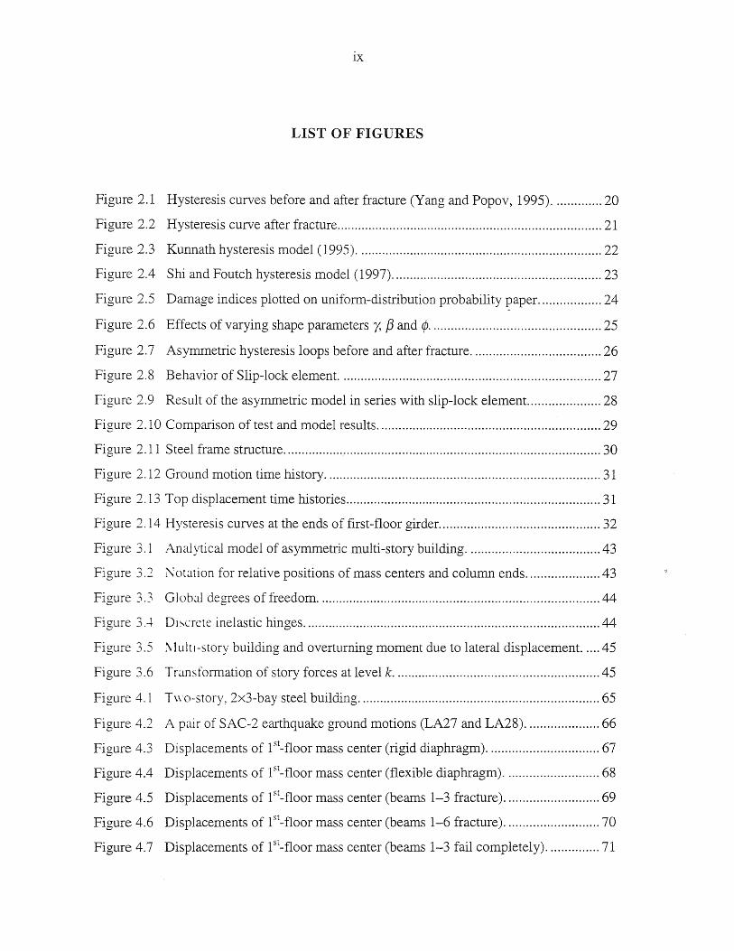
IX

LIST OF FIGURES

Figure 2.1 Hysteresis curves before and after fracture (Yang and Popov, 1995) .............. 20

Figure 2.2 Hysteresis curve after fracture ............................................................................ 21

Figure 2.3 Kunnath hysteresis model (1995) ...................................................................... 22

Figure 2.4 Shi and Foutch hysteresis model (1997) ............................................................ 23

Figure 2.5 Damage indices plotted on uniform-distribution probability paper. ................. 24

Figure 2.6 Effects of varying shape parameters y, f3 and ¢ ................................................. 25

Figure 2.7 Asymmetric hysteresis loops before and after fracture ..................................... 26

Figure 2.8 Behavior of Slip-lock element. .......................................................................... 27

Figure 2.9 Result of the asymmetric model in series with slip-lock element ..................... 28

Figure 2.10 Comparison of test and model results ................................................................ 29

Figure 2.11 Steel frame structure ........................................................................................... 30

Figure 2.12 Ground motion time history ............................................................................... 31

Figure 2.13 Top displacement time histories ......................................................................... 31

Figure 2.14 Hysteresis curves at the ends of first-floor girder. ............................................. 32

Figure 3.1 Analytical model of asymmetric multi-story building ...................................... 43

Figure 3.2 l\otation for relative positions of mass centers and column ends ..................... 43

Figure 3.3 GlohJ.l degrees of freedom ................................................................................. 44

Figure 3.-+ Dl~crete inelastic hinges ..................................................................................... 44

Figure 3.5 \ lulu-story building and overturning moment due to lateral displacement. .... 45

Figure 3.6 Transformation of story forces at level k . .......................................................... 45

Figure 4.1 Two-story, 2x3-bay steel building ..................................................................... 65

Figure 4.2 A pJ.ir of SAC-2 earthquake ground motions (LA27 and LA28) ..................... 66

Figure 4.3 Displacements of 1 st_ floor mass center (rigid diaphragm) ................................ 67

Figure 4.4 Displacements of 1 st_ floor mass center (flexible diaphragm) ........................... 68

Figure 4.5 Displacements of 1st-floor mass center (beams 1-3 fracture) ........................... 69

Figure 4.6 Displacements of 1 st_ floor mass center (beams 1-6 fracture) ........................... 70

Figure 4.7 Displacements of 1 st_ floor mass center (beams 1-3 fail completely) ............... 71

x

Figure 4.8 Displacements of 1 st-floor mass center (column 4 fails completely) ................ 72

Figure 4.9 Effects of connection fracture location on MCDR (2-story) with damage index

capacity uniformly distributed between 0.1 and 2.3 .......................................... 73

Figure 4.10 Effects of connection fracture location on MCDR (2-story) with damage index

capacity uniformly distributed between 0.1 and 0.5 .......................................... 74

Figure 4.11 Scatter of biaxial spectral acceleration (1; = 0.615, T2 = 0.496, S = 0.02 ) ........ 75

Figure 4.12 Biaxial spectral acceleration (1; = 0.615,T2 = 0.496,S = 0.02) plotted on log-

normal probability paper. ........................................................ ~ .......................... 75

Figure 4.13 Scatter of MCDR (2-story building) .................................................................. 76

Figure 4.14 Column drift ratios plotted on probability papers (2-story building) ................ 77

Figure 4.15 Three-story building ........................................................................................... 78

Figure 4.16 Scatter of biaxial spectral acceleration (1; = 0.851, T2 = 0.845, S = 0.02 ) ......... 79

Figure 4.17 Biaxial spectral acceleration (1; = 0.851, T2 = 0.845, S = 0.02) plotted on log-

normal probability paper. ................................................................................... 79

Figure 4.18 Scatter of MCDR (3-story building) .................................................................. 80

Figure 4.19 Column drift ratios plotted on probability papers (3-story building) ................ 81

Figure 4.20 Probability of exceedance vs. medians of MCDR ............................................. 82

Figure 5.1 Spectral acceleration hazard curve (2-story building) ....................................... 96

Figure 5.2 Regression of DI11 on Sa,m through three probability levels (2-story building).97

Figure 5.3 Regression of Dm on Sa,m through two probability levels (2-story building). 99

Figure 5 A Uniform hazard spectra .................................................................................... 101

Figure 5.5 Risk curves of maximum column drift ratio (2-story building) ...................... 102

Figure 5.6 Spectral acceleration hazard curve (3-story building) ..................................... 103

Figure 5.7 Regression of Dm on Sa,m through two probability levels (3-story building). 104

Figure 5.8 Risk curves of maximum column drift ratio (3-story) ..................................... 106

Figure A.1 Biaxial interaction under square displacement loading path (isotropic, post-

yield stiffness = 0, n = 2) .................................................................................. 115

Xl

Figure A.2 Biaxial interaction under square displacement loading path (orthotropic, post-


Figure A.3 Biaxial interaction under square displacement loading path (isotropic, post-to-

pre-yield stiffness ratio = 0.05, n = 2) .............................................................. 117

Figure A.4 Biaxial interaction under diamond displacement loading path (isotropic, post-







yield stiffness = 0, n = 10) ................................................................................ 121

Figure B.1 Numbering and member properties ................................................................. 127

Figure B.2 Global degrees of freedom ............................................................................... 127

Figure B.3 Member-end shears and bending moments ..................................................... 128

Figure B.4 Inelastic hinges ................................................................................................. 128

Figure C.1 2-DOF system ................................................................................................... 134

Figure C.2 Hysteresis curves of SA subjected to (a) LA33 only, (b) LA33 and LA34 .... 135

Figure C.3 Hysteresis curves of SA subjected to (a) LA39 only, (b) LA39 and LA40 .... 136

Figure CA A pair of SAC-2 earthquake ground motions (LA35 and LA36) ................... 137

Figure C.5 Displacement histories of floor mass centers under LA35 in X-direction ..... 138

Figure C.6 Hysteresis curves of column 8 under LA35 in X-direction ............................ 139

Figure C.7 Hysteresis curves of column 20 under LA35 in X-direction .......................... 140

Figure C.8 Hysteresis curves of column 32 under LA35 in X-direction .......................... 141

Figure C.9 Displacement histories of floor mass centers under LA36 in Y-direction ..... 142

Figure C.10Hysteresis curves of column 8 under LA36 in Y-direction ............................ 143

Figure C.11 Hysteresis curves of column 20 under LA36 in Y -direction .......................... 144

Figure C.12Hysteresis curves of column 32 under LA36 in Y-direction .......................... 145

Figure C.13 Displacement histories of floor mass centers under LA35 and LA36 ............ 146

XlI

Figure C.14Hysteresis curves of column 8 under LA35 and LA36 ................................... 147

Figure C.15 Hysteresis curves of column 20 under LA35 and LA36 ................................. 148

Figure C.16Hysteresis curves of column 32 under LA35 and LA36 ................................. 149

1

CHAPTER 1

INTRODUCTION

1.1 Background

-The welded steel moment frame buildings had long been regarded as one of the

most ductile systems because of moment-resisting beam-column joints in the lateral load

resisting systems. The welded moment-resisting joints, if fabricated in accordance with

the code procedures such as that of ANSI! A WS, were believed of having adequate

ductility capable of extensive plastic deformation without fracture failures.

After the 1994 Northridge earthquake and the 1995 Hyogoken-Nanbu earthquake,

however, many connection brittle-fracture failures have been found in welded steel

moment frame buildings. Since then, the investigation of cause and effect of brittle

connection fractures has been carried out in many institutions supported by the SAC steel

project, and the National Institute of Standards and Technology (NIST). SAC is a joint

venture of Structural Engineers Association of California (SEAOC), Applied Technology

Council (ATC), and California Universities for Research in Earthquake Engineering

(CUREe). The test results of steel connections thus far in the SAC project have verified

the post-earthquake field survey results and shown a large variability in the load carrying

capacity of these connections. In view of these recent findings, an urgent question faced

by the profession is what is the reliability and redundancy of a large number of such

structures in the building stock against future earthquakes. In other words, although very

few steel structures collapsed in these two earthquakes, the impact of possible brittle

connection failures on the performance of buildings against future earthquakes remains a

serious concern. There is clearly a need to investigate whether such structures have

enough reserve strength to survive future earthquakes.

2

Under earthquake excitations that are multi-dimensional in nature, member failures

or connection fractures may alter the dynamic properties of structures such as vibration

periods and mode shapes. Furthermore, torsional motions may become significant so that

structural response may be amplified considerably. To understand the structural behavior

under seismic loads, a dynamic structural analysis that can account for such effects is

required. Currently available computer programs such as DRAIN-2DX (prakash et aI.,

1993) and IDARC (Valles et aI., 1996), however, are primarily for analysis of plane

frames, and can not be used for study of torsional effect and biaxial bending interaction.

Also, analytical models are needed for brittle connection-fracture behavior.

Structural redundancy is a useful and perhaps most misunderstood concept among

structural engineers. Many factors affect structural redundancy, such as structural

configuration, load redistribution after partial failure, uncertainty in the structural

capacity versus that in the loading. The redundancy of structural systems under random

static loads has been investigated extensively in the past. For example, the concept of

system redundancy has been introduced to account for the additional load-carrying

capacity beyond first-member yielding (De and Cornell, 1990), or alternatively, the

availability of warning before the occurrence of collapse (Hendawi and Frangopol, 1994).

The redundancy of building structures under ground shaking has attracted more

attention after the Northridge and Hyogoken-Nanbu earthquakes. Very little, however, is

known on redundancy under stochastic dynamic loads primarily due to the analytical

difficulty associated with such problems. Most building code procedures do not

specifically deal with the effect of redundancy. Some recently proposed procedures (e.g.,

ATC-19, 1995; ICBO, 1997) introduce a new reduction of the response modification

factor depending on structural configuration (e.g., number of parallel lateral force

resisting structural components, ground floor area, and maximum element-story shear

ratio) based largely on judgment and experience. Further research is needed to have a

better understanding of redundancy that enables structural designers to evaluate and

design for the effect of redundancy on steel buildings under random loads.

3

1.2 Objective and Scope

The purpose of this study is to investigate the reliability and redundancy of low-rise

steel moment-resisting buildings under seismic excitation. The objectives are to:

1. Develop an analytical model for hysteretic behavior of fractured beam-to

column joints of steel buildings. The goal is to reproduce the global joint

hysteretic behavior observed in the SAC experiments.

2. Develop a three-dimensional building model for investigation of structural

behavior of steel buildings under seismic excitation. The emphasis is on effect

of biaxial interaction, torsional oscillation, and brittle beam-column joint

failures.

3. Propose a framework for evaluation of structural reliability and redundancy of

low-rise steel buildings under stochastic excitation. A uniform-risk redundancy

factor is proposed for use in structural design and performance evaluation.

1.3 Organization

In Chapter 2, experimental results of beam-column sub-assemblages and observed

hysteretic characteristics are reviewed. A smooth connection-fracture hysteresis model is

proposed. Based on the Bouc-Wen smooth hysteresis model (Wen, 1980), an additional

parameter is introduced to account for the asymmetry of the hysteresis loop. The model

is then put in series with a slip-lock element to account for pinching. It successfully

reproduces the main features of the force-displacement relationship of fractured joints,

such as the asymmetry of hysteresis loops, progressive degradation in strength or

stiffness, or both, pinching and spread of joint slip, large variability in energy-dissipating

capability before fracture, and shapes of hysteresis loop after fracture. Comparisons of

the SAC test data to the simulated results are made.

Chapter 3 describes the modeling of three-dimensional building structures

considering biaxial interaction, torsion, and brittle beam-column joint failures. Floor

4

diaphragms are assumed to be rigid in plane but flexible out-of-plane, which prohibits in

plane shear distortion and axial elongation but permits out-of-plane bending deformation.

Inelastic yielding is assumed to be confined to discrete hinge regions located at the

structural member (beam and column) ends. For beams, since the bi-axial interaction

effect is negligible the hinge yielding is restricted to occur only with respect to the

horizontal principal axis of the beam cross section subjected to bending moment. For

columns, each end is able to form one hinge with respect to each of the two principal axes

of its cross section. Therefore there can be two plastic hinges formed -on each beam and

up to four on each column. P-L1 effect is also considered.

Chapter 4 consists of response analyses of one two-story and one three-story steel

moment-resisting building subjected to ground motions of the SAC Phase 2 project using

the joint and structural building models developed in Chapters 2 and 3. Randomness of

material and member properties is considered. Effects of flexible diaphragm assumption

are investigated. Since the buildings are subject to bi-axial excitation, a definition of bi

axial spectral acceleration is proposed considering concurrently the dynamic properties in

the two principal directions of the building. For a given probability level of earthquake

occurrence, e.g., 10% in 50 years, it is found that the bi-axial spectral acceleration and

maximum column drift ratio, which will be used as a structural performance measure, can

be modeled as random variables with log-normal distribution. In order to examine the

effects of brittle connection fracture, bi-axial excitation, torsion, and column damage,

seven cases of different assumptions of member and system behavior are investigated and

compared.

In Chapter 5, a framework is presented for evaluation of structural reliability

against specified limit states in terms of maximum story (or column) drift. A redundancy

factor is proposed based on structural reliability for quantifying effect of redundancy on

buildings under earthquake excitations. The uncertainty in earthquake ground shaking is

described by the annual exceedance probability of spectral acceleration, approximately

modeled by a log-normal distribution. The relationship between spectral acceleration and

limit-state response such as maximum column drift ratio is then established by a simple

5

power law equation. The resistance and modeling uncertainty is considered by using a

uncertainty correction factor. The probability of exceeding a given limit-state is then

equal to that of the spectral acceleration corresponding to the limit-state multiplied by the

correction factor. Finally, a reliability-based redundancy factor is developed, which may

be used in a design formula.

Chapter 6 summanzes the conclusions of this study and recommendations for

future research.

6

CHAPTER 2

MODELING OF HYSTERETIC BEHAVIOR OF STRUCTURAL MEMBERS

2.1 Introduction

-Severe earthquake ground shaking often pushes structures into inelastic state. The

inelastic restoring forces are dependent not only on the instantaneous displacements but

also on the past loading history; besides, the structures may deteriorate in strength or

stiffness, or both, and exhibit pinching of the hysteresis loops because of damage to the

system. The resulting restoring force-displacement relation is, therefore, highly nonlinear

and hysteretic.

Accuracy of analysis of inelastic structural response under seismic loads depends

largely on the modeling of force-displacement relation. The currently available models of

the hysteresis loops are based on either fitting static or quasi-static cyclic test results (e.g.,

Clough and Johnston, 1966; Iwan, 1973; Takeda, Sozen, and Nielson, 1976), or

describing force-displacement relation by an approximate mathematical formulation (e.g.,

Nigam, 1969; Pecknold, 1974; Park, Wen and Ang, 1986).

After the 1994 Northridge and 1995 Hyogoken-Nanbu earthquakes, widespread

brittle beam-to-column connection fractures have been discovered in steel frame

structures. Since then studies of the cause and effect of brittle connection fractures have

been carried out in many institutions, for example, those supported by the SAC joint

venture of SEAOC, ATC, and CUREe. A few test results of fractured connections from

SAC are shown in Figure 2.1 and Figure 2.2. Several features of the force-displacement

characteristic can be observed: (1) the asymmetry of hysteresis loops, (2) progressive

strength or stiffness degradation, or both, (3) pinching and spread of pinching, and (4)

large variability in energy-dissipating capabilities before fracture and shapes of hysteresis

loop after fracture. Kunnath (1995) proposed a degrading hysteresis model for the

7

fractured connection behavior, as shown in Figure 2.3. This model only considers the

asymmetry and strength degradation after fracture, and therefore unable to simulate the

large variety of fractured connection behavior, as shown in Figure 2.1 and Figure 2.2. Shi

and Foutch (1997) proposed another piecewise-linear model (Figure 2.4), and

incorporated it into the DRAIN-2DX computer program as an additional element type. A

number of controlling parameters and rules are used in this model in order to fit the

hysteresis loops derived from experimental data. Since this model was developed

primarily as an extension to the DRAIN-2DX, it is not easy to use with other solution

methods.

The Bouc-Wen smooth hysteresis model (Wen, 1976 and 1980) has been widely

used for inelastic systems because of its capability of modeling a large variety of non

linearity, analytical tractability, and efficiency in computation. It has been used in time

history response analysis, equivalent linearization and random vibration analysis, as well

as structural control studies. The Bouc-W en model is therefore used herein as the basis to

describe the force-displacement and moment-rotation relationships observed in the cyclic

loading tests of fractured steel beam-to-column connections.

In the following, the capacity of connections against fracture failure will first be

discussed. Then the original Bouc-Wen model will be briefly described and a

modification of this model to account for the asymmetry of hysteresis loops will be

presented. Finally, a pinching element will be introduced and put in series with the

asymmetric element to model the connection fracture hysteresis.

2.2 Capacity of Moment-Resisting Connections Against Fracture

Cyclic loading test results of beam-column sub-assemblages revealed that even

though the connections were of the same material and member size, they exhibited

various rotational and energy dissipation capacities before fracture (e.g., Yang and

Popov, 1995). As shown in Figure 2.1, some connections failed in less than two cycles of

load test, others were able to withstand up to more than four cycles. The results imply

8

that the capacities of moment-resisting connections in a building could vary widely from

one to another.

Survey data (Youssef, Bonowitz and Gross, 1995) after earthquakes and

experimental results (Hajjar and Leon, 1996; Kaufinann, Di Julio, Jr. and Gross, 1997)

further indicated that fracture mostly originated from the bottom side of beam flanges.

Test results by Dang (1997), however, showed that the performance of top flange welded

joints are not much better than the bottom ones, and the cyclic performance under

dynamic loading testing is even poorer. Therefore it was argued that relatively rare

failures of the top flange welds found in field survey may due to the obstruction of floor

slabs and perimeter walls. It will be shown by numerical examples in Chapter 4,

however, that the influence of the location of fracture at top or bottom flange on

structural response may be negligible.

It is further found that besides the weld damage, extensive fractures sometimes

propagated into beam web or even column web and flange. Also, while the damage may

be severe, there is almost always some residual resistance at connections (SAC 96-01

Part 1, 1996). It is observed that when the fractured connection was bent in such a way

that causes the crack to open, the moment strength dropped to about 20% to 40% of the

original val ue. When it was bent to close the crack the strength only dropped to about

70% to 90~ 0 of its original strength.

As reponed by Youssef, Bonowitz and Gross (1995): "Connection performance

may be best understood in probabilistic terms with emphasis on construction and

inspection quality_" it therefore would be appropriate to model the capacities of

connections against fracture failures as random variables. Since the recorded data thus far

are quite limited on the amount of the residual strength of connections after fractures, the

statistical distribution of residual strength has not been established. In this study, a

uniform distribution is assumed for the reserve strength of both opening and closing

fractured connections.

A common measure of damage in analysis and design is the ductility factor,

defined as the ratio of maximum displacement to yield displacement. It is recognized,

9

however, that damage is caused not only by excessive displacement, but also through

cyclic load reversals. To include the cumulative damage, the hysteretic energy dissipation

can be used as a damage indicator. Park, Ang, and Wen (1984) proposed a damage index

as a linear combination of ductility and hysteretic energy dissipation:

(2.1)

where ID = damage index; ~m maximum displacement; ~um maXImum

displacement under monotonic loading; Eh = total dissipated hysteretic energy; Vy =

yield strength; and fJ = strength deterioration parameter counting for damage contribution

of the cumulative plastic strain energy. Although the model was originally developed and

verified against experimental results for RC members, results of small-scale tests (Chai,

Romstad, and Bird, 1995) show that it is also valid for steel members. The Park-Ang

damage index, therefore, will be used as a measure of the capacity against fracture

failure.

The capacity of a number of test results in terms of Park-Ang damage index is

shown in Figure 2.5. Figure 2.5(a) shows the probability distribution of eight damage

indices of cyclic loading tests performed by Engelhardt and Husain (1993), and Yang and

Popov (1995) Figure 2.5(b) is the results of 57 small-scale steel member tests (Chai,

Romstad. and Bird, 1995). Both are plotted on uniform distribution probability papers.

Figure 2.5 suggests that the connection fracture-resisting capacity may be modeled by a

random variable with an uniform distribution between 0.1 and 2.3. In the reliability

analysis. the random capacity measured by the damage index for each connection is

generated from the uniform distribution. In the response time history analysis, the

damage indices of connections are calculated at each time instant. Fracture at a particular

connection is assumed to occur at the time instant when its threshold value is exceeded.

10

2.3· Bouc-Wen Smooth Hysteresis Model

A smooth hysteresis model was first proposed by Bouc (1967) and later generalized

by Wen (1976), Baber and Wen (1981) for uniaxial force-displacement relation. The

model was subsequently generalized (Park, Wen and Ang, 1986) to account for the

effects of biaxial interaction.

2.3.1 Uniaxial Hysteresis Model

Consider a single-degree-of-freedom inelastic system, of mass m, damping c, and

initial elastic stiffness k, subjected to a base acceleration ug (t). The equation of motion

of the system can be written as

(2.2)

in which the restoring force q(u, z) can be expressed as

q(u,Z) = aku+(1-a)kz (2.3)

where u is the displacement of the system; a is the post-to-pre-yielding stiffness ratio; Z is

the hysteretic displacement and satisfies the following nonlinear differential equation:

z = ~{A - vlzln[13 sgn(uz) + r J} 17

(2.4)

in which A, 13, rand n are parameters controlling the shape of hysteresis; 17 and v are

parameters controlling the pre-yielding stiffness and ultimate strength, respectively.

Detailed discussions of the properties of parameters can be found in Baber and Wen

(1981) and Foliente (1995).

2.3.2 Biaxial Hysteresis Model

If a two-degrees-of-freedom inelastic system with translational mass m in two

orthogonal axes is subject to bi-directional excitations, ugx and Ugy ' in the two orthogonal

axes, then the equations of motion of the system along the two axes are:

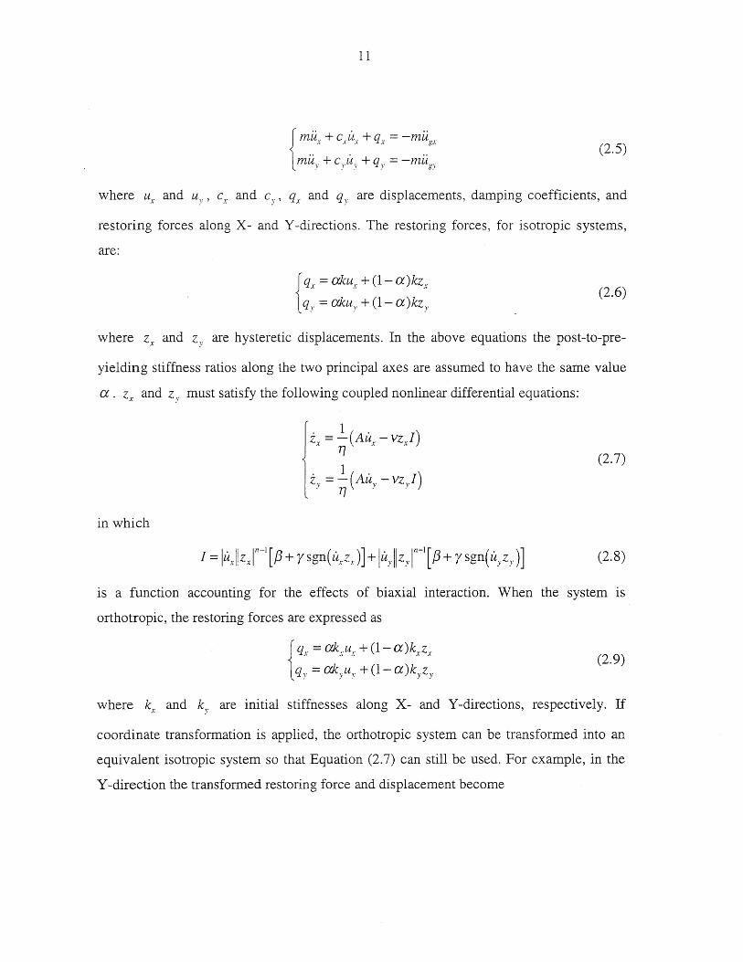
11

{ m.~x + CX~lX + qx = -m~gX muy + C)'u y + qy = -mug)'

(2.5)

where Ux and uy ' Cx and c)" qx and q)' are displacements, damping coefficients, and

restoring forces along X-and Y -directions. The restoring forces, for isotropic systems,

are:

{

qx = akux + (1- a)kzx

qy = akuy + (1- a)kzy (2.6)

where Zx and Zy are hysteretic displacements. In the above equations the post-to-pre

yielding stiffness ratios along the two principal axes are assumed to have the same value

a. Zx and Zy must satisfy the following coupled nonlinear differential equations:

7 = ~ (Au - Vz I) ~x x x

T]

. 1 (A· I) ZV = - u..,. -vzv . T] . -

(2.7)

in which

(2.8)

IS a function accounting for the effects of biaxial interaction. When the system is

orthotropic, the restoring forces are expressed as

{ qx." : akx. Ux + (1 = a)kxzx

q)' - akyUy + (1 a)kyzy (2.9)

where kx and ky are initial stiffnesses along X- and Y-directions, respectively. If

coordinate transformation is applied, the orthotropic system can be transformed into an

equivalent isotropic system so that Equation (2.7) can still be used. For example, in the

Y -direction the transformed restoring force and displacement become

12

, Fx qy =-qv . F .

y

, .6. Y =_x Y

.6. y

(2.10)

in which Fx ' Fy ' and .6. x , .6.)' are yield strengths and yield displacements, respectively,

in X- and Y-directions. It would be convenient to express the restoring forces and

displacements in the original coordinate system:

lqX = akxux + (1- a )kxz~

q, = akyu, +(l-a) ~y kyz; x

(2.11)

The transformed hysteretic displacements z.: and z~, are subsequently expressed as

0' l(AO 'I') z x = 17 u x - vz x

(2.12) 0' _ 1 (A.6. X

• 'I'J Zy -- -uv -vz, . 71 .6.' 0

'I Y

in which

I' = ILi,llz;j"-l[f3 + Y sgn(u,z~)l + ~x luy llzr1[f3 + ysgnhz~)] oV

(2.13)

When 11 = :2. Equation (2.12) reduces to the following form given by Park, Wen and Ang,

(1986):

(2.14)

Note that it is difficult to derive explicit relations between zx' Zy and z~, z~. The

interaction of forces in the two orthogonal directions is discussed in Appendix A. In this

study, n = 2 is used to model the biaxial bending interaction of columns.

13

2.3.3 Shape and Degradation Parameters

In the above formulation, the parameters /3, y, and n control the shape of the

hysteresis curves, whereas A, 17, and v control the deterioration of the system. For

deteriorating systems, the parameters A, 17, and v vary with time characterizing the

extent of structural damage and are assumed to be functions of dissipated hysteretic

energy:

jA=Ao-8AE

71 = 710 + 8TJE

v = vo +8vE

(2.15)

where Ao, 710 and Vo are initial values; 8 A' (7) and 8v are the rate of degradation. E is

the normalized dissipated hysteretic energy and evaluated as follows:

For uniaxial hysteresis model:

For biaxial hysteresis model:

E = 1- ex rtkz'udt FI1 Jo

2.4 Asymmetric Smooth Hysteresis Model

2.4.1 Constitutive Relations

(2.16)

(2.17)

The non-degrading hysteretic behavior generated by the Bouc-Wen model results in

equal ultimate positive and negative restoring forces. For some materials and

components, however, different ultimate values are often observed: For example, cast

iron, shape-memory alloy, and fractured beam-column connections. To model such

14

material and structural component behavior, a hysteretic model capable of accounting for

the asymmetry of peak restoring forces is required.

The Bouc-Wen model can be extended as follows to account for the asymmetric

yielding behavior:

i = ~{A - vlzlll[f3 sgn( ilz) + r + ¢(sgn( z) + sgn( it) )]} 17

(2.18)

in which ¢ is an additional parameter. To see the effect of ¢, consider the ultimate

hysteretic displacement, zu. When z -7 zu' i -7 0, it and z have the same sign.

Therefore,

A - Vlzu In (13 + r ± 2¢) = 0 1

Z" = [V(f3 + ~± 2~J (2.19)

The parameters 13, y, and ¢ are then appropriately chosen to describe the desired

hysteresis behavior. The hysteresis loops will shift downward or upward depending on

the sign (positive or negative) of parameter ¢. Effects of various values of 13, r, and ¢

are shown in Figure 2.6.

2.4.2 Shape Parameters of Fractured Beam-Column Connections

Assuming that before fracture, the shape parameters are 13, r, and ¢, the ultimate

positive and negative hysteretic displacements are ZUI and ZU2' respectively, as shown in

Figure 2.7(a). Then, from Equation (2.19),

(2.20)

Similarly, if we assume that after fracture, the shape parameters are [3', y', and ¢' , the

ultimate hysteretic displacements are cjzu1

and C2ZU2

' where c] and c2 are the ratios of

15

the ultimate hysteretic displacements after fracture to that before fracture, shown In

Figure 2.7(b) in which cj and c2 are 0.4 and 0.8, respectively. Therefore,

f3+y+2¢

(2.21)

Solving the above equations for 13' + y' and ¢' , one has

g' , 13 + y + 2¢ f3 + y - 2¢ J-I + Y = + -'--~-~

2c j

n 2c;

¢' = 13 + y + 2¢ _ f3 + y - 2¢ 4ct 4c;

(2.22)

Since there are three unknowns in two equations, it is necessary to choose an appropriate

ratio of f3' to y' for solving Equation (2.22).

Often linear force-displacement relation IS observed when a steel member is

unloading, one can assume that f3 = y and f3' = y', which give the desired behavior.

Besides, for a steel member with symmetric cross section, such as W -shape beams,

¢ = O. Equation (2.22) can then be simplified as follows:

(2.23)

Therefore, for a fractured steel beam-column connection with symmetric hysteresis curve

before fracture one can simply solve from Equation (2.23) to determine post-fracture

hysteretic parameters.

16

2.5 Slip-Lock Element

&

The force-displacement relationship of a variety of materials and structures, such as

smart materials, wood joints, and fractured steel structural joints, often exhibits slip

phenomenon. That is, the stiffness in a narrow low-force zone is very small, resulting in a

large displacement corresponding to a small increase of force. Outside the slip zone the

stiffness rapidly builds up, virtually preventing the element from further slipping. Ideal

behavior of slip-lock elements (Baber and Noori, 1985) is shown in Figure 2.9(b).

To determine the appropriate functional form of the slip-lock function, f( z) , let us

consider the force-displacement relation of the slip-lock element, Figure 2.9(b). If we

interchange the X- and Y-axes, the plot will be as shown in Figure 2.8(a). The

differentiation of ~ can be approximated by a bell-shaped function, Figure 2.8(b).

For mathematical tractability, the form of Gaussian density function, a bell-shaped

function, is selected for f( z). The following function is proposed:

[ ]

2

. (.) z sgn u --q 2 a 1 z fez) = [2 -exp __ u

~; (J 2 (J (2.24)

where the parameter a controls the length (or spread) of the pinching; (J controls the

sharpness of pinching; q denotes the fraction of Zu at which the stiffness reaches the

minimum, thus controlling the "thickness" of pinching area. After repeated trials, the

following function for a is recommended to model the hysteresis of fractured steel beam

column connections:

(2.25)

where ao is the initial length of pinching; 8 a is the rate of spread of pinching; E is the

normalized dissipated hysteretic energy as defined in Equation (2.16).

17

2.6 Smooth Connection-Fracture Hysteresis Model

Some typical hysteresis loops of fractured beam-to-column connections of steel

frames are shown in Figure 2.2, in which we can clearly see the asymmetry, slip, and

pinching of the hysteresis. To model these behaviors, the asymmetric hysteresis model is

put in series with a slip-lock element, as shown in Figure 2.9.

Denote ~ as the displacement of the asymmetric hysteresis element and ~ as that

of the slip-lock element. The total rate of change of displacement, it, is:

and the constitutive law of the asymmetric element, from Equation (2.18), is:

z =!!l{ A - vlzllt[f3 sgn( ~z) + y + ¢(sgn(z) + sgn(~))]} TJ

Assuming that the slip rate of the slip-lock element can be expressed as:

(2.26)

(2.27)

(2.28)

where fez) is the slip-lock function controlling the spread and the severity of pinching, ~

can be written as, from Equations (2.26) and (2.28):

~ = u-f(z)z (2.29)

Substitutin~ Equation (2.29) into Equation (2.27) and noting that

sgn(li) = ,,~n( II I = sgn(~), one obtains z as

in which

: = ~ {A - vlzlll[f3 sgn( itz) + Y + ¢( sgn( it) + sgn( z))]}. h(z) Tl

1 h(-)=--------------------------------------

~, 1+ fez) {A- vlzr[f3 sgn(itz)+y+¢(sgn(it)+sgn(z))]} TJ

(2.30)

(2.31)

18

is the pinching function. Note that when no slippage occurs and the hysteresis is

symmetric; i.e., a = 0, f(z) = 0 , and ¢ = 0, Equation (2.30) reduces to the original Bouc-

Wen model.

2.7 Applications

2.7.1 Reproducing Experimental Result

Some hysteresis curves from cyclic load tests of fractured beam-column

connections are shown in Figure 2.2. To reproduce the test results, one needs to know the

test setup, connection detailing, materials and properties, and exact forcing function. The

purpose of this section is to demonstrate the capability of the model in reproducing

important hysteretic behavior after fracture, such as asymmetry of hysteresis loops,

pinching, slip and spread of slip length. Therefore, employment of exact forcing function

used in cyclic test will not be attempted.

Figure 2.10 shows the comparison of a test result to its counterpart produced by the

proposed analytical model. Because the hysteresis characteristics under positive moment

may be different from that under negative moment, different sets of values of pinching

and degrading parameters for the two cases may be needed for satisfactory modeling. In

this example, the foHowing are assumed for a positive moment: ao = 2.0, 6 a = 1.6, with

no stiffness degradation. For a negative moment, ao = 3.0, 6a = 0.15, and both stiffness

and strength deteriorate with time. Parameters (J and q are 0.06 and 0.12, respectively,

for both positive and negative moments. Comparison of Figure 2.10(a) to Figure 2.10(b)

indicates that the proposed model reasonably reproduces the important hysteretic

properties of test data.

19

2.7.2 Response Analysis of Steel Frame with Fractured Connection

A one-bay, two-story steel frame is shown in Figure 2.11. The frame is under the

excitation of a ground motion record, LA27 from SAC phase 2 project (SAC Background

Document, 1997) for Los Angeles, California, shown in Figure 2.12. The displacement

time histories of the 2nd floor for events with and without connection fracture are shown

in Figure 2.13. The fracture failure is assumed to occur at the left joint of the first-floor

girder. For simplicity, the pinching and degradation parameters are assumed to have the

same values for the joint experiencing positive and negative moments; i.e., ao = 2.0,

o a = 0.45, () = 0.01, q = 0.06 . Both stiffness and strength deteriorate with time.

To determine the time instant at which connection fracture occurs, the Park-Ang

damage index (Park, Ang and Wen, 1984) introduced in Section 2.2 is used as a measure

of the capacity against fracture failure. A threshold value, 0.05, of the damage index is

assigned to the fractured connection. Fracture occurs at time t = 4.18 seconds.

Figure 2.13 shows that the frame with a fractured connection experiences

significantly larger response and permanent displacement. Period elongation can also be

observed. Figure 2.14 shows the hystereses of the joint with and without fracture. After

fracture, the girder end undergoes a larger rotation and has less energy-dissipating

capacity, resulting in a much larger displacement and permanent set of the frame, as seen

in Figure 2.13. An accurate modeling of the hysteretic behavior of fractured connection

is, therefore, necessary in successfully predicting the performance of steel frame

buildings with pre-Northridge beam-column connections.

20

("10~ SAC PH 1 TESTED RESPONSE SAC PN1 TESTED RESPONSE 1.0

2 0.5

Z

t '. I"

Y til 0-

S. :l' 0 i 0.0 .....

~ :lE :::E 0 0 :::E :::E

-2 -0.5

-1.0 -2 -1 0 1 2 -2 -1 0 1 2

TOTAl ROTAnON <X RAO) PLASnC ROTATION (X !WJ)

(al) (a2) (x'O~ SAC PN2 TESTED RESPONSE SAC PN2 TESTED RESPONSE

1.0

2 0.5

Z t I" til a.. :::E g. 0 "';:::- 0.0 g 15

:::E :::E 0 0 :::E ::I

-2 -0.5

-1.0 -2 -\ 0 1 -2 -1 0 1 2

TOT ..... RelATION <X RAO) PlASTlC ROTAnON (':I: RAO)

(bl) (b2) (,,'0~ SAC PN3 TESTED RESPONSE SAC PN3 TESTED RESPONSE

1.0

2

"-., ..... ,. f 0.5

"i 1 .;., . t;, c~

11. "'-.., :::E ~ ~ 0.0 7

I ~

:. :::E 0

~ :::E

-h -0.5

I

-1.0 -2 -1 0 , -2 -1 0 1 2

TOTAL ROTATION (X: RAO) PLASTIC ROTATION (X RAO)

(c1) (c2)

Figure 2.1 Hysteresis curves before and after fracture (Yang and Popov, 1995).

, . , '1./..i'#4(JO..Df)-j •••••••••••••

.... - .. - .......... - .... . . ,

Figure 2.3. Hysteretic behavior, specimen #1. (Anderson, Johnston, and Partridge, 1995)

{: aJ-IOCOOJIO.-I .. - -: - .... ~ .... ~ .......

I •

-- -~----:-- .r-----:


21

O.DoC

I \ • I ---: .... -~-- .. ~---~



Figure 2.2 Hysteresis curve after fracture.

M cr

M y

22

_ ~5M :-- - - - y- - - - - - - - - - - -

(a) Model Parameters

(b) Loop Behavior

strength drop

Figure 2.3 Kunnath hysteresis model (1995).

Moment

Mt+-P2 ~

Mg + - - - - - - -; - -:- - -;- - -

-~ : 13 .

23

24

Rotation

---- DYNAMIC PATH

•••• STATICPATH

Figure 2.4 Shi and Foutch hysteresis model (1997).

24

2.5 • 2.0

x (l.)

u 1.5 c: (l.) b1) c-;j

E 1.0 c-;j

Cl

0.5

0.0 0.0 0.2 0.4 0.6 0.8 1.0

Cumulative probability

(a) Damage indices of eight cyclic loading test results.

1.8

1.7

x ...::: 1.6

":..J ~

1.5

1.4

1.3

1.2 0.0 0.2 0.4 0.6 0.8 1.0

Cumulative probability

(b) Damage indices of fifty-seven small-scale test results.

Figure 2.5 Damage indices plotted on uniform-distribution probability paper.

25

(a) y + f3 > 0, y - f3 = 0, ¢ > 0. (b) Y + f3 > 0, y - f3 = 0, ¢ < ° .

(c) y + f3 > 0, y - f3 < 0, ¢ > 0. (d) Y + f3 > 0, y - f3 > 0, ¢ > 0.

(e) Y+f3=O, y-f3<O, ¢>O. (f) y + f3 = 0, y - f3 < 0, ¢ < 0.

Figure 2.6 Effects of varying shape parameters y, f3 and cp.

26

(a) Before fracture.

(b) After fracture.

Figure 2.7 Asymmetric hysteresis loops before and after fracture.

27

Figure 2.8 Behavior of Slip-lock element.

28

z

z

z

u

Figure 2.9 Result of the asymmetric model in series with slip-lock element.

-3

29

100.00 t

~.oot

T

I T

-,::: ~ -'50.00 1

load. kips

Displacement. in

(a) Test result (Anderson, et al., 1995).

100

(b) Model result.

Figure 2.10 Comparison of test and model results.

3

-~ ~

30

W24x68

W24x68

Fractured connection

25'

Figure 2.11 Steel frame structure.

0\ tn ~

X ~ ~

~

31

1.0

~ 0.5 Q)

U 0.0 u

<r: -0.5

-1.0 10 15 20

Time (sec)

Figure 2.12 Ground motion time history.

15

:::: 10 ~ 0.. Cf.J .-Q

-5 10 15 20

Tim e (sec)

(a) Without connection fracture.

15

c:: 10 ~

Ci, Cf.J

0 -5

0 10 15 20

Time (sec)

(b) With a connection fracture.

Figure 2.13 Top displacement time histories.

32

600 600

400 400

,-. 200 ~

200 ~ "--" 0 c o ClJ ~ 0 -200 ~

-200

-400 -400

-600 -600 -0.06 -0.04 -0.02 0.00 0.02 -0.06 -0.04 -0.02 0.00 0.02

Rotation (rad) Rotation (rad)

Left end Right end

(a) No fracture.

600 600

400 400

~ 200 ~

200 ~ '---'

0 o

~ -200 ~

-200

-400 -400

-600 -600 -OOE -0.04 -0.02 0.00 0.02 -0.06 -0.04 -0.02 0.00 0.02

Rotation (rad) Rotation (rad)

Left end Right end

(b) Left end fractures at time t = 4.18 seconds.

Figure 2.14 Hysteresis curves at the ends of first-floor girder.

33

CHAPTER 3

MODELING OF ASYMMETRIC MULTI-STORY BUILDINGS

3.1 Introduction

Analysis of structural response requires mathematical model of the structures. This

is one of the most critical components in structural analysis, since the accuracy of the

calculated results depends on how well the mathematical model represents the behavior

of real structural system.

A building is a three-dimensional structure. Dynamic analysis of three-dimensional

systems generally requires a large and costly computer program, therefore in practice the

modeling of a real physical system is often simplified by certain assumptions to obtain

results with acceptable accuracy at a reasonable cost. A structure with a regular,

symmetric configuration and uniform mass distribution may be modeled as two

dimensional frame structure without much loss of accuracy. In many cases, however,

biaxial interaction may arise as a result of structural irregularity or torsional oscillations,

affecting significantly the response under seismic excitation. For example, mass

eccentricity. irregular layout such as setback, and fractured beam-to-column connections

can cause biaxial interaction. Besides, recorded earthquake accelerograms indicate that

the ground motion is basically three-dimensional, and the motions in the three principal

directions do not have a strong correlation (Kubo and Penzien, 1976). In such cases, two

dimensional models are no longer adequate.

Yeh and Wen (1989) employed a model for asymmetric multi-story buildings in

which the floor diaphragms were assumed to be rigid so that plastic deformation can

occur only in the columns. The recent design philosophy, however, encourages strong

column, weak-beam designs to prevent the occurrence of inelastic distortions in the

columns. In addition, to account for the effects of connection fractures one needs to

34

model the girders with reasonable flexibility and moment-resisting capacity. It IS

necessary, therefore, that the floor diaphragms remain flexible in the modeling of

building structures.

When a structure yields, the yielding locations can, in principle, form at any

stressed regions. For instance, if there is a large gravity load at the mid-span of girders,

hinges are likely to form at mid-span. In the case of building structures under earthquake

excitation, however, lateral deflections usually dominate and generate large concentrated

stresses in the regions of beam-to-column connections. Krawinkler (i 996) proposed an

inelastic connection model consisting of three rotational springs. One of which is the

"panel zone spring," representing the stiffness and deformation of panel zones, the other

two represent the properties of beams connecting to the joint. As pointed out in Shi

(1997), drawbacks of this model are: (1) In many cases, the strength of panel zones is less

than the strength of beams, once a panel zone yields, plastic deformation will be

restricted to the panel zone spring. (2) The connection behavior is tested and recorded

based on the integral performance of the joint configuration, and the beam and panel zone

performance can not be easily separated. Therefore, in this study the inelastic

deformation of structures will be assumed to concentrate at regions adjacent to beam

column connections and modeled as discrete inelastic hinges at column and girder ends.

The property of the inelastic hinges is specified in accordance with the force

displacement hysteresis behavior of the integral joint configuration, as discussed in the

preceding chapter.

3.2 Equations of Motion

An asymmetric multi-story building with mass eccentricity is shown in Figure 3.l.

Each floor diaphragm, of mass Mi and moment of inertia Ii' is assumed to be rigid in its

own plane but flexible out-of-plane, which is a reasonable assumption for the floor

system (U ang, 1997). By this assumption, the motion of the diaphragm at each floor level

35

can be characterized by 3 rigid-body degrees of freedom in its own plane, i.e., translation

in the X and Y directions, plus a rotation about the vertical axis.

In addition, because the floor diaphragms are flexible out-of-plane, the column

ends are allowed to rotate with respect to both X- and Y-axes. As a result, two additional

rotational degrees of freedom at each column end are required. Therefore, if the axial

deformation of members is neglected, the vector of structural (global) degrees of freedom

is given by

u = ( .. ···f - (3.1)

in which u~, u~. and u~ are the relative displacements and in-plane rotation of the ith floor

relative to the ground; 8~~ and 8;' are the column-end rotations of the /h column on the ith

floor. The global displacement vector U of a one-story structure is shown in Figure 3.3.

The initial position of the ith floor mass center is (m~, m~.) , and that of the /h column

on the ith floor is (e;, e;), both of which are measured with respect to the global

coordinate system as shown in Figure 3.1. Since, in general, the rotation of floor

diaphragms is small, it can be assumed that the relative end-displacements of the ith -floor

columns in X-and Y -directions are linear functions of i i-J i-J d i-J ue ' Ux ' uy ,an ue ;

that is:

d iJ _ i i-J (ij i) i + (iJ H) H x - Ux - Ux - e y - my Ue e y - my Ue

_ i _ i-J_V iJ ,i+ Tii H - Ux Ux y ~ e Ly Ue

d u = i _ i-J +( ij _mi)ui -(eU _mH)uH y uy uy ex x e x x e

(3.2)

_ i i-J V iJ i TiJ i-J - uy - uy + x Ue- Lx Ue

in which V and L are used to denote the relative positions of a column to its upper- and

lower-floor mass centers respectively, as shown in Figure 3.2.

The translational accelerations of the ith - floor mass center along X-and Y-axes are

U~ + ugx and u~. + Ugy , where ugx and Ugy are ground accelerations. If the rotational

36

component of ground acceleration is neglected, then the rotational acceleration of the ith

floor is u~. The equations of motion for the ith-floor diaphragm can therefore be

expressed as:

M.··i+~Sij-(l-5:'. )~S(i+l)k=_M.·· lUX .L..,; x U IN .L..,; x IUgx

j k

M .u··i +~Sij -(1- 5:'. )~S(i+l)k =-M.·· I)" .L..,; Y U IN.L..,; Y IUgy (3.3)

j k

liU~ + L stU - (1- 6 iN) L S~i+l)k,B = 0 j k

where S; and S; are the shears of the /h column on the ith floor along X- and Y

directions, respectively; stU denotes the torsional resistance of column j on the ith floor

to its upper floor; S~i+l)k,B is the torsional resistance of column k on the (i+l)th floor to its

lower floor; 6 iN is the Kronecker delta; and N is the total number of floor diaphragms. If

the upper- and lower-floor mass centers of a column do not align in a vertical axis, the

relati ve distances of the column to the two mass centers will be different. As a result,

stU and stB will be different.

It is further assumed that inertial resistance to rotation at column-end nodes is small

and can be neglected, thereby in dynamic analysis the rotational degrees of freedom at

the column-end nodes can be eliminated by static condensation. After performing static

condensation. the equations of motion for the building structure are expressed as follows:

(3.4)

in which 1'1 is the lumped-mass matrix including the translational masses and rotational

moments of inertia of diaphragms; iia is the acceleration vector at the mass centers of

diaphragms relative to the ground; iig is the vector of ground acceleration; S is the vector

of column-end shears; the matrix J:\. adds up the column-end shears acting at a particular

floor diaphragm, as well as the torsion induced by those shears. Note that damping forces

that have not been included will be added later.

37

3.3 Discrete Hinge Yielding Model

Consider a multi-story building with yielding confined to discrete hinge regions.

Theoretically, these hinges may occur at arbitrary locations. For a moment-resisting

frame structure subjected to earthquakes, however, yielding often concentrates at beam

and column-end regions. Therefore, in such case the hinge locations will be restricted to

regions immediately adjacent to beam-column joints. For beams, because the biaxial

interaction effect is negligible, the hinge yielding is restricted to occur only with respect

to the horizontal principal axis of the beam cross section subjected to bending moment.

For columns, in order to account for the biaxial interaction, two hinges can form at each

column end with respect to the two principal axes of the column cross section; therefore

there may be up to four plastic hinges on one column. Figure 3.4 shows the likely formed

plastic hinges for a one-story structure.

The displacement vector U can be partitioned into two component vectors: ua

consisting of all the degrees of freedom with inertia and U c consisting of those without

inertia. That is:

Ua = (- .. i u~. i .. -)T Ux Uz

Uc; = (. .. eU eU .. -)T x y

(3.5)

Besides global displacements ua and u c ' the plastic hinges also produce a vector

of hinge rotations, h. The rotational deformations of hinge elements at a joint are

generally different from one to another, as shown in Figure 3.4. The member-end

rotations at jointj are the joint rotations minus that of the connecting plastic hinges. Thus

the vector of member-end forces can be expressed as:

IS) [Kss Ksc]{ } [KSH] R = K RS K RC :: - KRH {h-z} H KHS KHC KHH

(3.6)

In which z is the hysterestic component of hinge rotation; S = column-end shears;

R = member-end moments at ends without hinges; and H = member-end moments at

38

ends with hinges; the two stiffness matrices in brackets relate the member-end forces to

the global and hinge displacements.

By equilibrium, the member-end moments H should be equal to the hinge-element

moments, i.e.:

(3.7)

where Ke and K z are coefficient matrices of hinge moments. Vector z is obtained from

the smooth hysteresis model,

z = g(it,z) (3.8)

Details of g have been discussed in Chapter 2. It is noted that the uniaxial hysteresis and

connection-fracture models are used to model the moment-rotation relations on beams,

whereas the biaxial model is used to model those on columns. Since rotational masses are

not present at joints, rotational equilibrium at joints may be expressed in terms of only the

member-end moments as follows:

(3.9)

where the matrix TR is for summing up the end moments present at a particular joint.

Examining Equations (3.4) and (3.6) to(3.9), one can show that the number of unknowns

(which are u a ' u c ' hand z) equals the number of equations. Therefore the dynamic

response of a building is completely described by these equations.

Defining the following variables

(3.10)

and substituting the 2nd and 3rd rows of Equation (3.6) into Equation (3.9), one can solve

for U c as follows:

(3.11 )

39

Equating the right-hand side of the 3rd row of Equation (3.6) to that of Equation (3.7), and

replacing U c by Equation (3.11), one obtains

(3.12)

where

{QJ = KHC(TRKECflTRKES -K HS Q2 = Ke +KHH -KHC(TRKECfITRKEH

(3.13)

Substituting Equation (3.11) and the 1st row of Equation (3.6) for S into Equation (3.4),

one can express the equations of motion as:

(3.14)

where

jQ3: Ts[Kss - Ksc(T~~EctTRKES 1 Q4 - Ts[ Ksc(TRKEC) TRKEH - KSH]

(3.15)

Combining Equations (3.12) and (3.14) into matrix form, one obtains the system of

equations of motion excluding damping terms as follows:

(3.16)

If Rayleigh damping is assumed and has the following form:

(3.17)

in which ao and a l are proportionality constants, then Equation (3.16) becomes

(3.18)

Setting a state-variable vector y and its derivative as

40

(3.19)

one can solve Equations (3.8) and (3.18) numerically for y by using any appropriate

solution methods for a system of first -order ordinary differential equations such as

Runge-Kutta and Rosenbrock methods (Press, Teukolsky, Vetterling, and Flannery,

1992), for given initial conditions, and obtain the response time history. The assembly of

relevant stiffness matrices and coefficient matrices for modeling a simple one-bay, one

story building is illustrated in Appendix A.

3.4 p-~ Effects

A building structure needs to sustain lateral displacement under earthquakes. If the

lateral displacement becomes large, the secondary moments caused by story weights may

further increase the displacement such that stability becomes a concern. For evaluation of

structural response under severe earthquake shaking, it would be necessary to consider

this secondary effect to obtain an acceptable estimate of response.

In this study, consideration of P-~ effects generally follows the technique proposed

by Wilson and Habibullah (1987). Consider a multi-story building with mass centers

aligned in a vertical line, as shown in Figure 3.5. The building is subjected to a

displacement in X-direction. Story i, of story weight Wi' and story height li' has a

displacement u~. The secondary moment caused by Wi is

= w· .6. + ~- +. ··+8 ( I ') . )

I x x X

i

= w.~ f!,.k 1L-J x k=1

(3.20)

where ~kx is the inter-story drift of story k. Equation (3.20) is equally applicable to Y-

direction. Assuming that the radius of gyration of the mass at story i is 'i, then the

41

equivalent shear forces and torsion induced by the displacements and rotation of floor

diaphragm at story i can be shown (Wilson and Habibullah, 1987) to be

pi w· . 1 1 =-ux x li

pi Wi i (3.21) =-uv y l. -1

p/ Wi 2 i

e = [If Ue 1

The overturning moment M~ can be distributed to story i and all stories below

story i according to Equation (3.20). Thus at story k, k = 1 to i , the forces are written as

/ /

pi k-l Xk-l 1 0 0 -1 0 0

Ux / /

pi Yk-I 0 1 0 0 -1 0

k-J Uy

/ /

pi 0 0 2 0 0 2 k-J ek_

1 Wi If -If Ue

p: lk -1 0 0 1 0 0 k

Ux k

0 -1 0 0 1 0 k ~)ik 0 0 2 0 0 2

Uy -If If

(3.22)

pi ek

k Ue

or symbolically,

/ , P~ =(K~). u~

C lk (3.23)

The prime denotes that the quantities are at a location directly below the centroid of story

i, as shown in Figure 3.6. It is common that the centroid at all story levels is not in a

vertical alignment; therefore the forces must be transformed to the centroid of story k by

the following calculation:

42

pi pi

1 0 0 0 0 0 Xk-l

xk-l pi pi 0 1 0 0 0 0 Yk-l

Yk-l

pi -(Yi - Yk-l) (Xi -Xk- 1) 1 0 0 0 pi ek- 1 = ek - 1

pi 0 0 0 1 0 0 ,

xk pi

P.:k 0 0 0 0 1 0

xk

pi pi 0 0 0 -(Yi - Yk) (Xi-Xk ) 1 Yk ek

(3.24)

pi ek

or symbolically,

(3.25)

Similarly, the displacements u~ can be expressed in terms of the displacements at the

centroid, Uk' by the following:

(3.26)

Combining Equations (3.23), (3.25), and (3.26), one gets

(3.27)

in which

(3.28)

(K g) ik needs to be calculated for every i = 1 to Nand k = 1 to i and summed up to obtain

a geometric matrix Kg; that is,

(3.29)

The displacement amplification caused by p-~ effects on low-rise buildings,

however, is not as significant as that on high-rise buildings. For a low-rise building

subjected to large lateral displacement, the impact of geometric non-linearity may be

more important.

L

43

• Locations of mass centers

Figure 3.1 Analytical model of asymmetric multi-story building.

(C U cU) --:;;r--/ ------------------------- --;:1- x' y .~ / /

// // / /

/

( /-1 /-1) //

/ /

m ,my /-1 /

_______________ !!~ __ // At rest

r/ x During vibration

Figure 3.2 Notation for relative positions of mass centers and column ends.

44

® e:A ~----------~~

x

Figure 3.3 Global degrees of freedom.

Figure 3.4 Discrete inelastic hinges.

ONG VARIOUS DESIGN CRITERIA FOR! PRESTRESSED CONCRETE

Documents

Transcript of ONG VARIOUS DESIGN CRITERIA FOR! PRESTRESSED CONCRETE