One-year monitoring of the Z24-Bridge: environmental effects versus damage events

EARTHQUAKE ENGINEERING AND STRUCTURAL DYNAMICSEarthquake Engng Struct. Dyn. 2001; 30:149–171

One-year monitoring of the Z24-Bridge: environmental e�ectsversus damage events

Bart Peeters∗;† and Guido De Roeck

Department of Civil Engineering; Katholieke Universiteit Leuven; W. de Croylaan 2; B-3001 Heverlee; Belgium

SUMMARY

When using the analysis of vibration measurements as a tool for health monitoring of bridges, theproblem arises of separating abnormal changes from normal changes in the dynamic behaviour. Normalchanges are caused by varying environmental conditions such as humidity, wind and most important,temperature. The temperature may have an impact on the boundary conditions and the material properties.Abnormal changes on the other hand are caused by a loss of sti�ness somewhere along the bridge.It is clear that the normal changes should not raise an alarm in the monitoring system (i.e. a falsepositive), whereas the abnormal changes may be critical for the structure’s safety. In the frame of theEuropean SIMCES-project, the Z24-Bridge in Switzerland was monitored during almost one year beforeit was arti�cially damaged. Black-box models are determined from the healthy-bridge data. These modelsdescribe the variations of eigenfrequencies as a function of temperature. New data are compared with themodels. If an eigenfrequency exceeds certain con�dence intervals of the model, there is probably anothercause than the temperature that drives the eigenfrequency variations, for instance damage. Copyright ?2001 John Wiley & Sons, Ltd.

KEY WORDS: vibration monitoring; temperature e�ect; damage detection; system identi�cation; automaticmodal analysis

1. INTRODUCTION

Since many years people are performing vibration tests on civil engineering structures. Itbecame more and more clear that environmental parameters a�ect the dynamic behaviour of astructure. For instance, the Young’s modulus of concrete decreases with increasing temperature.Also the boundary conditions may be temperature-dependent. Damage detection is one ofthe main aims of vibration monitoring. A loss of sti�ness is observed as a decrease of theeigenfrequencies. The problem is that changes due to damage can be completely masked

∗ Correspondence to: Bart Peeters, Department of Civil Engineering, Katholieke Universiteit Leuven,W. de Croylaan 2, B-3001 Heverlee, Belgium.

† E-mail: [email protected]

Received 4 January 2000Revised 14 March 2000

Copyright ? 2001 John Wiley & Sons, Ltd. Accepted 18 May 2000

150 B. PEETERS AND G. DE ROECK

by changes due to normal varying environmental parameters. Owing to their local charac-ter, the occurrence of damage or a boundary condition change have a selective in uence onthe eigenfrequencies. A temperature change, a�ecting the global material properties, has auniform in uence on the eigenfrequencies. Therefore damage identi�cation methods that takeinto account this selective frequency in uence may still work in the presence of temperaturevariations.Alampalli [1] reports that the relative eigenfrequency di�erences (�f) of a bridge due to

freezing of the supports (�f=40–50 per cent) were an order of magnitude larger than changesdue to damage (�f=3–8 per cent), which was in this case an arti�cial saw cut across thebottom anges of both girders. It must be mentioned that the studied bridge was relativelysmall, with a span of 6:76m and a width of 5:26m and it was tested using an impact hammer.Roberts and Pearson [2] described a monitoring program on a 9-span, 840m long bridge. Theyfound that normal environmental changes could account for changes in eigenfrequencies of asmuch as 3–4 per cent during the year. Farrar et al. [3] found that the �rst eigenfrequencyof the Alamosa Canyon Bridge varies approximately 5 per cent during a 24 h time period. Ina paper by Sohn et al. [4], the same bridge data are used to build a regression model thatdescribes the variation of eigenfrequencies due to varying temperatures. The model is used toestablish con�dence intervals of the frequencies for a new temperature pro�le. R�ucker et al.[5] showed that the temperature e�ects on the dynamics of a 7-span highway bridge in Berlincan also not be neglected. Finally, Askegaard and Mossing [6] found that a 3-span footbridgeexhibits normal frequency variations of 10 per cent during the year.This paper presents the results of (almost) one year monitoring of the Z24-Bridge. The

main contributions of the paper are the following:

• An automatic modal analysis (AMA) procedure, based on stochastic subspace identi�cation,is proposed that is able to extract the modal parameters from stabilization diagrams withoutany user interaction. The fact that the procedure could be automated is a key issue in acontinuous monitoring system.

• By carefully inspecting the available data, the physical phenomenon behind the typicalbilinear relation between frequency and temperature is identi�ed.

• Due to the relatively large amount of data, a more detailed data analysis is possible ascompared to the classical statistical regression analysis, where a relation is establishedbetween simultaneously measured data. In this paper, we tried to �nd dynamic models thatrelate measurements at di�erent time instants.

• A quite unique data set [7] could be used to validate the proposed method. Unique in asense that measurements are available for all four seasons and that the bridge could bedamaged at the end of the monitoring period. We are showing that it is indeed possible to�lter out the environmental variations and we are able to detect the damage.

The paper is organized as follows. Next section describes the bridge and the monitoring system.Section 3 explains how the modal parameters are automatically extracted from the massiveamount of vibration data. In Section 4, we attempt to construct black-box models that explainthe variation of the eigenfrequencies due to changing environmental in uences. The modelsare found by applying system identi�cation techniques to the data of the undamaged bridge. InSection 5, the models are validated by using fresh data. These validation data also contain thearti�cial damage events. Finally some conclusions and recommendations are given in Section 6.

Copyright ? 2001 John Wiley & Sons, Ltd. Earthquake Engng Struct. Dyn. 2001; 30:149–171

ENVIRONMENTAL EFFECTS VERSUS DAMAGE EVENTS 151

Figure 1. The Z24-Bridge: longitudinal section and top view [7].

Figure 2. Cross-section of the Z24-Bridge and location of the thermocouples. The variablei is the span number; i=1; 2; 3 [7].

2. THE Z24-BRIDGE AND THE EMS

The Z24-Bridge is located in Switzerland, connecting the villages Utzenstorf and Koppigenand overpassing the national highway A1 between Bern and Z�urich. It is a classical post-tensioned concrete box girder bridge with a main span of 30m and 2 side spans of 14m(Figure 1). Two rows of three pinned concrete columns are supporting the bridge at the endpoints and two concrete piers clamped into the girders are situated at the end points of themain span. The bridge is slightly skew. Although there were no known structural problemswith the bridge, it had to be demolished because a new railway next to the highway requireda bridge with a larger side span.From 11 November 1997 till 11 September 1998, the bridge has been monitored. The

aim of the environmental monitoring system (EMS) is to provide both environmental andvibration data. 49 Sensors captured environmental parameters such as air temperature, windcharacteristics, humidity, bridge expansion, soil temperatures at the boundaries and bridge



Figure 3. (Top) Air temperature; (Bottom) Soil temperature at one of the piers. The representedmeasurement period is from 11-Nov-1997 till 20-Apr-1998. The sampling time is 1 h.

Figure 4. Typical acceleration data. (Top) time history; (Bottom) power spectral density estimate byWelch’s method. The sampling time is 0.01 s.

concrete temperatures. The locations of the bridge thermocouples are shown in Figure 2. Thesampling time is 1 h: every hour, data from all sensors were captured simultaneously. Figure3 shows the air temperature and the soil temperature at one of the piers. The soil temperaturevariations are much smoother. Additionally, every hour during 11mins, eight accelerometerscapture vibrations of the bridge. Typical acceleration data in time and frequency domain areshown in Figure 4. More details on the bridge and the EMS can be found in Kr�amer et al.[7; 8] and Rushton et al. [9].



3. AUTOMATIC MODAL ANALYSIS (AMA)

As indices for the dynamic behaviour of the structure, it is natural to take the modal parame-ters: eigenfrequencies, damping ratios, mode shapes. Evidently, a realistic vibration monitoringsystem should be able to estimate the modal parameters from output-only data. There is nopossibility of continuously exciting the bridge with a known force; so we have to use availablebut unmeasurable sources such as tra�c and wind. An excellent method for the estimation ofmodal parameters from output-only data is stochastic subspace identi�cation (SSI). This timedomain method was developed in 1991 by Van Overschee and De Moor [10; 11]. Applica-tions to modal analysis appeared in 1995 [12; 13]. The method is implemented in the toolboxMACEC [14] for use with Matlab [15]. Advantages of SSI over the widely used frequencydomain peak-picking method are:

• The eigenfrequencies are objectively selected based on stabilization diagrams instead oflooking at peaks in the spectral densities of the signals.

• The damping estimates are far more reliable.• True mode shapes are obtained instead of operational de ection shapes.• Closely spaced modes can be separated.

Especially this last advantage is important in case of Z24-Bridge, since two closely spacedmodes are situated in the range 10–11Hz. It turned out that an automated peak-picking methodfailed to estimate both [9].SSI as it is implemented in MACEC requires some user interaction: the user has to select

stable frequencies based on stabilization diagrams. This is a serious problem for the presentcase: there are 10 CDs containing zipped acceleration data, measured at 5652 time instants.The interpretation of 5652 stabilization diagrams would take weeks and does not �t in arealistic monitoring system. Therefore an automatic modal analysis (AMA) procedure neededto be developed. The following steps are repeated 5652 times (for every data set). A certainidenti�ed pole is considered as stable if the frequency, damping and mode shape deviationswith respect to a pole identi�ed at one model order lower, are within certain limits. This isnothing more yet than the classical way of constructing a stabilization diagram. The automaticprocedure goes further and tries to incorporate the decisions that an experienced user wouldtake. Only poles that are ns times stable are selected (to exclude accidentally stable poles) andthe representative of a column of stable poles at a certain frequency is the one that is closestto the average of that column. The used criteria are:

�f61 per cent; ��610 per cent; 100 per cent× (1−MAC)65 per cent; ns¿5 (1)

where �f is the relative frequency di�erence, �� is the relative damping ratio di�erence andMAC is the modal assurance criterion, a measure of the correlation between two mode shapes.It is typical that the eigenfrequencies are the most accurately estimated modal parameters,whereas the damping ratios have the largest uncertainty. This is re ected in the stabilizationcriteria (1).From preliminary modal surveys [16], we know that we can expect four modes in the

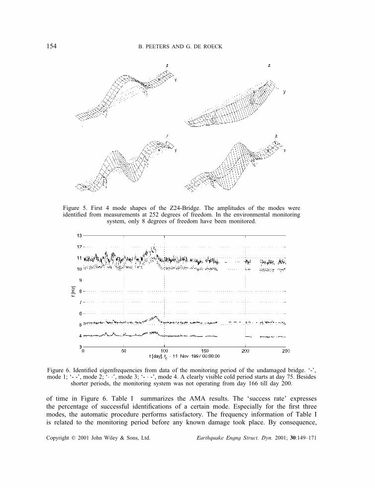
range 0–12Hz. The mode shapes are shown in Figure 5. However due to the sometimes lowexcitation (especially at night when there is not much tra�c) the AMA could not identifyall four modes at every time instant. The identi�ed eigenfrequencies are plotted as a function



Figure 5. First 4 mode shapes of the Z24-Bridge. The amplitudes of the modes wereidenti�ed from measurements at 252 degrees of freedom. In the environmental monitoring

system, only 8 degrees of freedom have been monitored.

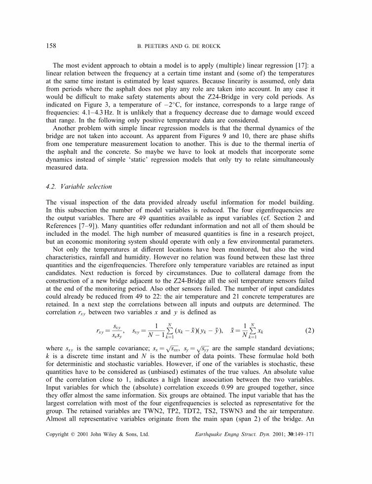
Figure 6. Identi�ed eigenfrequencies from data of the monitoring period of the undamaged bridge. ‘-’,mode 1; ‘- -’, mode 2; ‘· ·’, mode 3; ‘- · -’, mode 4. A clearly visible cold period starts at day 75. Besides

shorter periods, the monitoring system was not operating from day 166 till day 200.

of time in Figure 6. Table I summarizes the AMA results. The ‘success rate’ expressesthe percentage of successful identi�cations of a certain mode. Especially for the �rst threemodes, the automatic procedure performs satisfactory. The frequency information of Table Iis related to the monitoring period before any known damage took place. By consequence,



Table I. Automatic modal analysis results for the healthy structure. The minimum, averageand maximum frequencies are speci�ed, together with the relative maximal di�erence.

Mode Success rate (%) Eigenfrequency

Min (Hz) Avg (Hz) Max (Hz) Max. di�. (%)

1 98 3.81 4.00 4.38 142 93 4.98 5.21 5.89 183 96 9.60 10.16 11.20 164 77 10.24 10.84 12.09 17

the frequency di�erences ranging from 14 to 18 per cent have to be explained by normalenvironmental changes. If we would wait until damage makes the eigenfrequencies to exceedthe normal range, it would probably be too late.

4. BLACK-BOX MODELS: EIGENFREQUENCIES VERSUS TEMPERATURE

From November till the end of July, we assume that the bridge remains intact. These EMSdata are used to build experimental black-box models that relate the measured eigenfrequenciesto observed environmental parameters. An alternative to this approach would be a detailedanalysis of the physics that cause the eigenfrequencies to change. For instance a tempera-ture change a�ects the Young’s modulus, E, of concrete and asphalt; and the eigenfrequen-cies are proportional to the square root of Young’s modulus: f∼√

E. Also freezing of thesoil changes the boundary conditions of a structure [1] and these a�ect again the eigenfre-quencies. However, it may be clear that �nding a quantitative description of all involvedphysical phenomena is far too complex. So we preferred the black-box system identi�cationapproach. In this section, the search for a good model that is able to describe the data isdiscussed.

4.1. Visual inspection of the data

The �rst step in system identi�cation is taking a look at the data. The �rst eigenfrequencyversus the temperature of the wearing surface, TP1, is represented in Figure 7. The secondeigenfrequency versus the temperature of the deck so�t, TDS2, is represented in Figure 8.The relation between temperature and frequency can roughly be described by two lines, withthe knee situated around 0◦C. This bilinear behaviour is observed for almost all combina-tions of frequency versus temperature. Mode 2 is somewhat an exception in the sense thatits frequency increases with increasing temperatures (for positive temperatures). Some e�ortwas spent in trying to �nd out the cause of the bilinear behaviour. Whereas the temperatureversus time functions are very smooth; the frequency versus time functions are rather irregu-lar. This can be observed in Figure 9, where three di�erent temperatures and the opposite ofthe �rst eigenfrequency, (−1)×f, are plotted as a function of time. All quantities have beennormalized. At �rst sight there seems to be no relation between frequency and temperature.Although, on a larger time scale it would be clear that the frequency follows the main trends



Figure 7. 1st Eigenfrequency vs. wearing surface temperature, TP1. Data from the healthy structure.

Figure 8. 2nd Eigenfrequency vs. deck so�t temperature, TDS2. Data from the healthy structure.

of the temperature data. However, if we look at the data of a cold period (Figure 10), thenormalized opposite frequency is almost perfectly in line with the normalized temperature ofthe wearing surface (asphalt layer), TP1. The central web temperature, TWC1, and the so�ttemperature, TS1, are lagging behind and can by consequence not be the driving forces of theeigenfrequency variation. Also freezing of the soil around the boundaries of the bridge cannotexplain the variations. The soil temperature has a much lower-frequency content (Figure 3)than the eigenfrequencies (Figure 10). In this paper the eigenfrequencies are considered as a



Figure 9. Normalized temperatures and opposite of the 1st eigenfrequency (-f1) during a warm period.‘-’, TP1; ‘- -’, TWC1; ‘- · -’, TS1; ‘-+-’, -f1.

Figure 10. Normalized temperatures and opposite of the 1st eigenfrequency (-f1) during a cold period.‘-’, TP1; ‘- -’, TWC1; ‘- · -’, TS1; ‘-+-’, -f1.

time series of measurement values, so it makes sense to speak about the frequency content ofthe eigenfrequencies. We conclude that during warm periods, the asphalt does not play anyrole, but during cold periods, it contributes signi�cantly to the sti�ness of the structure. Thisexplains the non-linearity (Figures 7 and 8).



The most evident approach to obtain a model is to apply (multiple) linear regression [17]: alinear relation between the frequency at a certain time instant and (some of) the temperaturesat the same time instant is estimated by least squares. Because linearity is assumed, only datafrom periods where the asphalt does not play any role are taken into account. In any case itwould be di�cult to make safety statements about the Z24-Bridge in very cold periods. Asindicated on Figure 3, a temperature of −2◦C, for instance, corresponds to a large range offrequencies: 4.1–4:3Hz. It is unlikely that a frequency decrease due to damage would exceedthat range. In the following only positive temperature data are considered.Another problem with simple linear regression models is that the thermal dynamics of the

bridge are not taken into account. As apparent from Figures 9 and 10, there are phase shiftsfrom one temperature measurement location to another. This is due to the thermal inertia ofthe asphalt and the concrete. So maybe we have to look at models that incorporate somedynamics instead of simple ‘static’ regression models that only try to relate simultaneouslymeasured data.

4.2. Variable selection

The visual inspection of the data provided already useful information for model building.In this subsection the number of model variables is reduced. The four eigenfrequencies arethe output variables. There are 49 quantities available as input variables (cf. Section 2 andReferences [7–9]). Many quantities o�er redundant information and not all of them should beincluded in the model. The high number of measured quantities is �ne in a research project,but an economic monitoring system should operate with only a few environmental parameters.Not only the temperatures at di�erent locations have been monitored, but also the wind

characteristics, rainfall and humidity. However no relation was found between these last threequantities and the eigenfrequencies. Therefore only temperature variables are retained as inputcandidates. Next reduction is forced by circumstances. Due to collateral damage from theconstruction of a new bridge adjacent to the Z24-Bridge all the soil temperature sensors failedat the end of the monitoring period. Also other sensors failed. The number of input candidatescould already be reduced from 49 to 22: the air temperature and 21 concrete temperatures areretained. In a next step the correlations between all inputs and outputs are determined. Thecorrelation rxy between two variables x and y is de�ned as

rxy=sxysxsy

; sxy=1

N − 1N∑k=1(xk − �x)(yk − �y); �x=

1N

N∑k=1xk (2)

where sxy is the sample covariance; sx=√sxx; sy=

√syy are the sample standard deviations;k is a discrete time instant and N is the number of data points. These formulae hold bothfor deterministic and stochastic variables. However, if one of the variables is stochastic, thesequantities have to be considered as (unbiased) estimates of the true values. An absolute valueof the correlation close to 1, indicates a high linear association between the two variables.Input variables for which the (absolute) correlation exceeds 0.99 are grouped together, sincethey o�er almost the same information. Six groups are obtained. The input variable that has thelargest correlation with most of the four eigenfrequencies is selected as representative for thegroup. The retained variables are TWN2, TP2, TDT2, TS2, TSWN3 and the air temperature.Almost all representative variables originate from the main span (span 2) of the bridge. An



important remark is that a low correlation can also mean that there is just a time delay betweentwo signals, so it is possible that the six retained variables still contain some redundancy.

4.3. ARX models

Having reduced the number of possible input candidates to 6, we are ready to build an input–output model. The simplest model described in the system identi�cation literature (see forinstance Reference [18]) is the ARX model that consists of an auto-regressive output and aneXogeneous input part:

yk + a1yk−1 + · · ·+ anayk−na = b1uk−nk + b2uk−nk−1 + · · ·+ bnbuk−nk−nb+1 + ek (3)

where yk is the output — in this case an eigenfrequency — at time instant k; uk is the input— in this case a temperature — and ek is the equation error term modelling the disturbancesthat act on the input–output process. Typical sources for the disturbances are unknown inputsand measurement noise. This term is not known, but it is assumed that it is white noise,with zero mean E[ek]= 0 and covariance E[ekek−i]= ��i, where �i is the Kronecker symbol(i=0⇒ �i=1; i 6=0⇒ �i=0). E[•] is the expected value operator. In order to be able toestablish con�dence intervals, later in this paper, we also assume that ek is Gaussian distributed.The ARX model (3) is characterized by three numbers: na, the auto-regressive order; nb, theexogeneous order and nk , the pure time delay between input and output. The orders na and nbdetermine the number of model parameters: ai (i=1; : : : ; na); bj (j=1; : : : ; nb). By introducingthe shift operator, q−1yk =yk−1, and de�ning the operator polynomials

a(q)=1 + a1q−1 + · · ·+ anaq−nab(q)= b1q−nk + b2q−nk−1 + · · ·+ bnbq−nk−nb+1

(4)

the ARX model (3) can be written as

a(q)yk = b(q)uk + ek (5)

In general, parametrized linear input–output models are written as [18]

yk =G(q; �)uk +H (q; �)ek (6)

where � contains the model parameters, G is the transfer function and H is the noise model.In the ARX case, we have

�T = (a1 : : : ana b1 : : : bnb)

G(q; �)=b(q)a(q)

; H (q; �)=1a(q)

(7)

What makes ARX models so popular is that the parameters, �, can be estimated by simplelinear least squares. The estimate is denoted as �. A ‘static’ regression model is an ARX010model (with [na; nb; nk]= [0; 1; 0]):

yk = b1uk + ek (8)

Note that the means are removed from the input–output data; otherwise there would be ano�set in Equations (3) and (8). The advantage of using general ARX models over static



Table II. Comparison between SISO models: TDT2 — eigenfrequency.

Mode ARX model Static regression model

na nb nk � FPE na nb nk � FPE

1 2 1 4 0.145 0.145 0 1 0 0.212 0.2132 3 2 0 0.533 0.536 0 1 0 0.896 0.8973 2 1 0 0.507 0.509 0 1 0 0.548 0.5494 2 2 0 0.569 0.572 0 1 0 0.612 0.613

regression models is that they include some dynamics: the current output and input are relatedto outputs and inputs at previous time instants. If more than 1 input variable is included,Equation (3) is still valid but uk is a column vector and the b-coe�cients are row vectors.With a lot of input candidates and the possible choices for na; nb; nk there are many di�erentARX models that can be �tted to the data. By consequence criteria are needed that assess andcompare the quality of models. The least-squares method minimizes the sum of squares of theequation errors ek . A �rst-quality criterion is thus the value of the loss function, de�ned as

�=1N

N∑k=1�2k(�) (9)

with the estimated equation errors (the residuals) de�ned as

�k(�)= a(q)yk − b(q)uk (10)

The loss function is also an estimate of the noise covariance �, therefore the symbol � couldbe used. The problem of using the loss function as a quality criterion is that it continuouslydecreases as the model order increases. Other criteria include penalties for model complexitylike Akaike’s �nal prediction error (FPE) criterion or Rissanen’s minimum description lengthcriterion [18].

4.4. Application to the monitoring problem

Our strategy to �nd a good model is the following. For all four eigenfrequencies and remainingsix input candidates, single-input single-output (SISO) ARX models are estimated. A good andsimple (i.e. with only a few parameters) model is selected for each of the 24 input–outputcombinations, according to the quality criteria of previous section. Next, the input is selectedthat yields on the average the best models for all four frequencies. The best models havethe lowest � (9) and FPE values. It turned out that the model based on TDT2 performedbest; but it must be added that not much quality loss was observed when using any of thetemperatures TWN2, TP2 or TS2. The results are represented in Table II. The input and outputdata were normalized before the models were identi�ed. The model for the �rst mode seemsto be much better than the models for the other three modes. The static regression results arealso represented. Especially for the �rst two modes, the improvements of an ARX model overa static model are spectacular.Afterwards input variables were added to the SISO models, but it was observed that the

models hardly improved. For instance, the quality measures of a multiple-input single-output(MISO) ARX214 model, that includes all six input variables and has the �rst eigenfrequency



Figure 11. Normalized autocorrelation of the residuals of the TDT2 - f1 models: ‘- -’,ARX214; ‘-’, ARX010.

as output, are: �=0:142, FPE=0:143. These values have to be compared with the values onthe �rst line of Table II. For a static MISO ARX010 model that includes all input variables, wehave: �=0:187; FPE=0:188. It is not only more expensive to measure many temperatures, butalso not necessary. Multiple static linear regression does not perform better that single-inputARX modelling (0:187¿0:145).Another quality criterion for a model is provided by the covariance function of the residuals.

In order to justify the least-squares approach for �nding the model parameters, it was assumedthat ek is white noise: the covariances, Re(i), at time lags i di�erent from zero, have to bezero:

Re(i)=E[ekek−i]= ��i (11)

They are estimated as

Re(i)=1N

N∑k=1�k(�)k−i(�) (12)

In Figure 11, the auto-correlation functions Re(i)=� of the SISO ARX214 and ARX010 modelsare plotted; together with the 99 per cent con�dence intervals. The sequence of residuals ofthe static model is not white noise at all. This is an indication that more information can beextracted from the data.The ARX models were identi�ed from normalized data. They can be converted to engineer-

ing units. We applied following normalization:

yk =ymk − �ysy

; uk =umk − �usu

(13)

where the superindex m denotes a quantity in engineering units: (◦C) or (Hz). As usual,�y; �u are the sample means and sy; su are the sample standard deviations (2). By introducing



Equation (13) in Equation (5), the converted ARX model reads

a(q)ymk = b(q)sysuumk + syek + C (14)

where the o�set C is computed as

C= a(1) �y − b(1) sysu�u (15)

All necessary values to obtain these ‘engineering units’ ARX models are given in Appendix A.

5. VALIDATION: IS DAMAGE DETECTION POSSIBLE?

Once a good model is obtained, it can be used for simulation. New temperature measurementsare fed to the models and they simulate the eigenfrequencies of the Z24-Bridge. Note that insystem identi�cation one speaks of simulation if only input information is used to estimatethe outputs. If next to the inputs, also the outputs up to some previous time instant are usedto estimate the current output, one speaks of prediction. If the simulated eigenfrequencies aredeviating too much from the measured ones, something happened to the bridge that cannotbe explained by temperature e�ects. If for instance the measured frequencies are lower, thebridge could be damaged. The statement ‘deviating too much’ is a rather subjective criterionto judge the state of a structure. We need a more objective statistical criterion.

5.1. Statistical properties of the estimated models

From Appendix A and Reference [18], we know that not only the model parameters, but alsotheir covariances can be estimated from the data. From this covariance matrix P� and by a �rst-order approximation, the covariances of the simulated outputs can be estimated. This idea willbe developed in the following. We start with the general parametrized input–output model (6):

yk =G(q; �)uk +H (q; �)ek (6)

It is assumed that the ‘true’ system can be described by the model structure of Equation (6):

yk =G(q; �0)uk +H (q; �0)e0k (16)

where �0 are the ‘true’ model parameters and e0k are the actual disturbances with covariance�0. Based on the input–output data, the model parameters are estimated by prediction errormethods [18]. The estimate is denoted as �. In case of an ARX model, the prediction errormethod corresponds to the linear least-squares method. The noise-free simulated outputs fromthe estimated model are written as

yk =G(q; �)uk (17)

We examine the statistical properties of the di�erence between the true output (16) and thesimulated one (17):

dk = yk − yk =G(q; �0)uk +H (q; �0)e0k −G(q; �)uk= (G(q; �0)uk −G(q; �)uk) +H (q; �0)e0k (18)



The term between brackets can be expanded as a Taylor series. Only the �rst-order term isretained:

dk = J (q; �0)uk(�0 − �) +H (q; �0)e0k (19)

where the row vector J (q; �0) is de�ned as

J (q; �0)=@G(q; �)@�

∣∣∣∣�=�0

(20)

Since �→ �0 as N→∞, E[e0k]= 0 and e0k is Gaussian distributed, it follows from Equation(19) that dk is asymptotically Gaussian distributed with zero mean, E[dk]= 0, and a certaincovariance: E[(dk)2]=Pdk . This is denoted as

dk ∼N(0; Pdk ) (21)

An expression for Pdk is now derived. For notational clarity, we simplify: J0 = J (q; �0),H0 =H (q; �0). Inserting Equation (19) into the de�nition of the covariance Pdk yields

Pdk =E[(dk)2]=E[(J0uk(�0 − �) +H0e0k)((�0 − �)T(J0uk)T +H0e0k)] (22)

Since uk is deterministic, we have

∀i : E[uke0k−i] = ukE[e0k−i] = 0 (23)

The noise contribution is written as

v0k =H0e0k (24)

By inserting Equations (23) and (24) in Equation (22), following expression is obtained:

Pdk = J0ukE[(�0 − �)(�0 − �)T](J0uk)T + E[(v0k)2] (25)

It is possible to write the row vector J0uk outside the expectation operator, since it is adeterministic sequence. The covariances of the stochastic sequence v0k are de�ned as

R0v(i)=E[v0kv0k−i] (26)

By introducing the asymptotic covariance matrix of the model parameters P� and (26), wehave

Pdk = J0ukP�(J0uk)T + R0v(0) (27)

In Appendix B, it is shown how this asymptotic covariance of the simulation error can beestimated. From Equation (21), we have

yk − yk√Pdk

∼ N(0; 1) (28)

The true Pdk is not known. If it is replaced by its estimate Pdk , the Student’s t-distributionshould be used instead of the normal distribution. The 100(1−�) per cent con�dence intervalon yk (the true value) is given by

[yk − t�=2;�√Pdk ; yk + t�=2;�

√Pdk ] (29)

where t�=2;� is found from a statistical table of the Student’s t-distribution. The symbol � isthe number of degrees of freedom of the data after modelling; it equals �=N −d, with d, the



Figure 12. Mode 1 results. Simulation errors of the ARX214 model for TDT2 - f1 andthe 95 per cent con�dence intervals.

number of model parameters: d=dim(�). For a large number of data points, N , and �=0:05,we have t�=2;�=1:96. The signi�cance of the 95 per cent con�dence interval is that 95 percent of these intervals (29) will contain the true value yk .

5.2. Application to the monitoring problem

In previous section, an objective criterion was established that determines whether a simulatedfrequency, yk , determined by the temperature history, is deviating too much from the measuredone, yk . We are now ready to validate the method. The data which were already used toidentify the ARX models, and also new data, are fed to the models to yield the simulatedfrequencies and the 95 per cent con�dence intervals. The simulation errors together with the

[−t�=2;�√Pdk ; t�=2;�

√Pdk ] intervals are plotted in Figures 12–15. If a simulation error exceeds

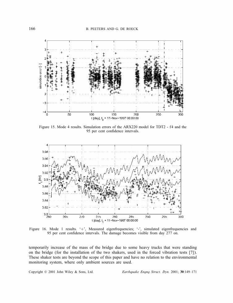
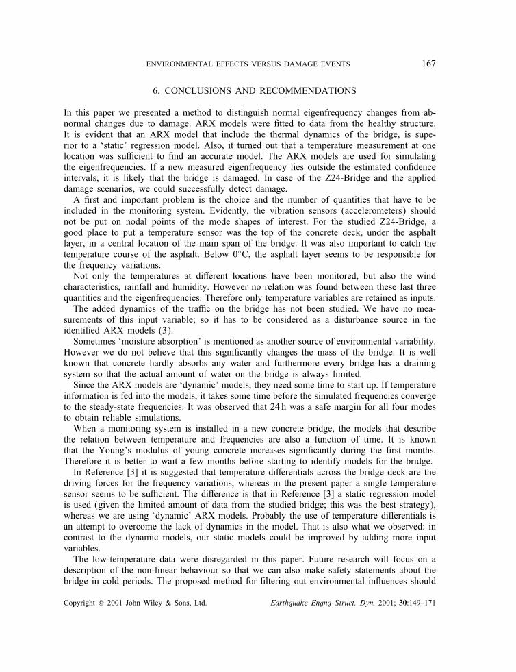
the interval, it is likely that something happened to the bridge. The vertical lines on the�gures split the residuals in two parts: an estimation and a validation part. The estimationdata were already used to estimate the ARX model, whereas the validation data are fresh data.Concerning mode 1, damage is observed from day 277 on (15 August 1998). Around this date,the damage scenario ‘Settlement of a pier, 80 mm’ was realized [7]. The preceding scenarios,settlements of 20 and 40mm, seem to have no large in uence on mode 1. The comparisonbetween the simulated and measured �rst eigenfrequency is made in Figure 16. Apart fromthe time span, this �gure is basically giving the same information as Figure 12. The di�erenceis that instead of the di�erence between the (normalized) measured and modelled frequencies,the frequencies (Hz) themselves are shown. The represented data show the surpassing of thecon�dence limits. For the other modes 2,3 and 4, damage is observed from day 269, 270on (7,8 August 1998). Around these dates, the settlement system was installed. The bridge



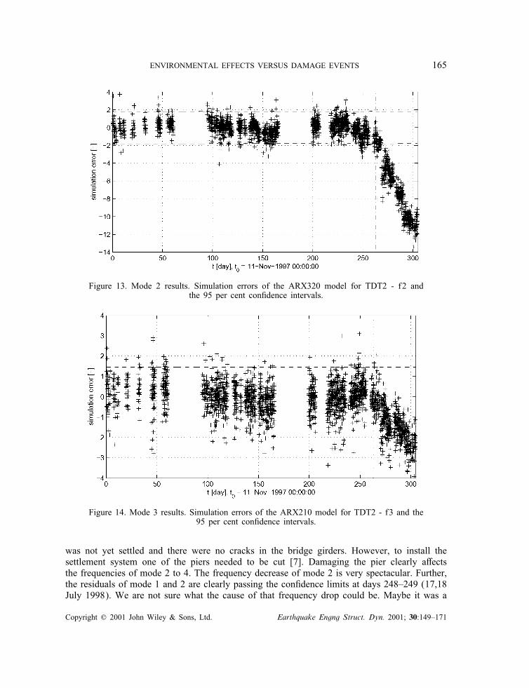
Figure 13. Mode 2 results. Simulation errors of the ARX320 model for TDT2 - f2 andthe 95 per cent con�dence intervals.

Figure 14. Mode 3 results. Simulation errors of the ARX210 model for TDT2 - f3 and the95 per cent con�dence intervals.

was not yet settled and there were no cracks in the bridge girders. However, to install thesettlement system one of the piers needed to be cut [7]. Damaging the pier clearly a�ectsthe frequencies of mode 2 to 4. The frequency decrease of mode 2 is very spectacular. Further,the residuals of mode 1 and 2 are clearly passing the con�dence limits at days 248–249 (17,18July 1998). We are not sure what the cause of that frequency drop could be. Maybe it was a



Figure 15. Mode 4 results. Simulation errors of the ARX220 model for TDT2 - f4 and the95 per cent con�dence intervals.

Figure 16. Mode 1 results. ‘+’, Measured eigenfrequencies; ‘-’, simulated eigenfrequencies and95 per cent con�dence intervals. The damage becomes visible from day 277 on.

temporarily increase of the mass of the bridge due to some heavy trucks that were standingon the bridge (for the installation of the two shakers, used in the forced vibration tests [7]).These shaker tests are beyond the scope of this paper and have no relation to the environmentalmonitoring system, where only ambient sources are used.



6. CONCLUSIONS AND RECOMMENDATIONS

In this paper we presented a method to distinguish normal eigenfrequency changes from ab-normal changes due to damage. ARX models were �tted to data from the healthy structure.It is evident that an ARX model that include the thermal dynamics of the bridge, is supe-rior to a ‘static’ regression model. Also, it turned out that a temperature measurement at onelocation was su�cient to �nd an accurate model. The ARX models are used for simulatingthe eigenfrequencies. If a new measured eigenfrequency lies outside the estimated con�denceintervals, it is likely that the bridge is damaged. In case of the Z24-Bridge and the applieddamage scenarios, we could successfully detect damage.A �rst and important problem is the choice and the number of quantities that have to be

included in the monitoring system. Evidently, the vibration sensors (accelerometers) shouldnot be put on nodal points of the mode shapes of interest. For the studied Z24-Bridge, agood place to put a temperature sensor was the top of the concrete deck, under the asphaltlayer, in a central location of the main span of the bridge. It was also important to catch thetemperature course of the asphalt. Below 0◦C, the asphalt layer seems to be responsible forthe frequency variations.Not only the temperatures at di�erent locations have been monitored, but also the wind

characteristics, rainfall and humidity. However no relation was found between these last threequantities and the eigenfrequencies. Therefore only temperature variables are retained as inputs.The added dynamics of the tra�c on the bridge has not been studied. We have no mea-

surements of this input variable; so it has to be considered as a disturbance source in theidenti�ed ARX models (3).Sometimes ‘moisture absorption’ is mentioned as another source of environmental variability.

However we do not believe that this signi�cantly changes the mass of the bridge. It is wellknown that concrete hardly absorbs any water and furthermore every bridge has a drainingsystem so that the actual amount of water on the bridge is always limited.Since the ARX models are ‘dynamic’ models, they need some time to start up. If temperature

information is fed into the models, it takes some time before the simulated frequencies convergeto the steady-state frequencies. It was observed that 24 h was a safe margin for all four modesto obtain reliable simulations.When a monitoring system is installed in a new concrete bridge, the models that describe

the relation between temperature and frequencies are also a function of time. It is knownthat the Young’s modulus of young concrete increases signi�cantly during the �rst months.Therefore it is better to wait a few months before starting to identify models for the bridge.In Reference [3] it is suggested that temperature di�erentials across the bridge deck are the

driving forces for the frequency variations, whereas in the present paper a single temperaturesensor seems to be su�cient. The di�erence is that in Reference [3] a static regression modelis used (given the limited amount of data from the studied bridge; this was the best strategy),whereas we are using ‘dynamic’ ARX models. Probably the use of temperature di�erentials isan attempt to overcome the lack of dynamics in the model. That is also what we observed: incontrast to the dynamic models, our static models could be improved by adding more inputvariables.The low-temperature data were disregarded in this paper. Future research will focus on a

description of the non-linear behaviour so that we can also make safety statements about thebridge in cold periods. The proposed method for �ltering out environmental in uences should



be validated on other bridges too. The approach followed in this paper is highly related to theproblem of detecting outliers. The authors are currently investigating the application of methodsfrom the statistical process control literature (e.g. Reference [19]) wherein these problems arediscussed.

ACKNOWLEDGEMENTS

The data for this research were obtained in the framework of the BRITE-EURAM Programme CT960277, SIMCES with a �nancial contribution by the European Commission. Partners in the projectwere: K.U. Leuven, Aalborg University, EMPA, LMS International, WS Atkins, Sineco, T.U. Graz.[http:==www.bwk.kuleuven.ac.be=bwm=SIMCES.htm].

APPENDIX A: IDENTIFIED MODELS

The identi�ed ‘engineering units’ ARX models have the following structure (14):

a(q)ymk = b(q)sysuumk + syek + C (14)

where the o�set C is computed as (15)

C= a(1) �y − b(1) sysu�u (15)

This appendix gives the estimated parameters and their estimated standard deviations. The dataproperties �u; su; �y; sy (13) are speci�ed in Table AI. The ARX model parameters are given inTable AII. The static regression parameters are shown in Table AIII. The least-squares methoddoes not only provide estimates, �, of the model parameters, �, but also an estimate, P�, ofthe asymptotic (i.e. for N→∞) covariance matrix of these parameters, P�. The speci�edestimated standard deviations ��i of the model parameters are the square roots of the maindiagonal elements of P�. See also Ljung [18]. The standard deviations are a measure of theaccuracy of the estimate. If some parameters have a large relative standard deviation, it ispossible that the model ‘over�ts’ the data and that too many parameters have been includedin the model.

APPENDIX B: ASYMPTOTIC COVARIANCE OF THE SIMULATION ERROR

The asymptotic covariance of the simulation error equals (27):

Pdk = J0ukP�(J0uk)T + R0v(0) (27)

None of the expressions at the right-hand side are known. They have to be estimated.

B.1. Model parameter covariance matrix estimate: P�

P�, an estimate of P�, follows from the statistical properties of the least-squares method thatwas used to �nd � (Appendix A).



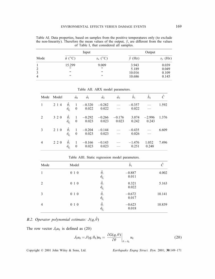
Table AI. Data properties, based on samples from the positive temperatures only (to excludethe non-linearity). Therefore the mean values of the output, �y, are di�erent from the values

of Table I, that considered all samples.

Input Output

Mode �u (◦C) su (◦C) �y (Hz) sy (Hz)

1 15.299 9.009 3.943 0.0392 ” ” 5.189 0.0493 ” ” 10.016 0.1094 ” ” 10.686 0.145

Table AII. ARX model parameters.

Mode Model a0 a1 a2 a3 b1 b2 C

1 2 1 4 �i 1 −0:320 −0:282 — −0:357 — 1.592��i 0 0.022 0.022 — 0.022 —

2 3 2 0 �i 1 −0:292 −0:266 −0:176 3.074 −2:996 1.376��i 0 0.023 0.023 0.023 0.242 0.243

3 2 1 0 �i 1 −0:204 −0:144 — −0:435 — 6.609��i 0 0.023 0.023 — 0.026 —

4 2 2 0 �i 1 −0:166 −0:143 — −1:476 1.052 7.496��i 0 0.023 0.023 — 0.251 0.248

Table AIII. Static regression model parameters.

Mode Model b1 C

1 0 1 0 �i −0:887 4.002��i 0.011

2 0 1 0 �i 0.321 5.163��i 0.022

3 0 1 0 �i −0:672 10.141��i 0.017

4 0 1 0 �i −0:623 10.839��i 0.018

B.2. Operator polynomial estimate: J (q; �)

The row vector J0uk is de�ned as (20)

J0uk = J (q; �0)uk =@G(q; �)@�

∣∣∣∣�= �0

uk (20)



In case of an ARX model, the transfer function equals (7)

G(q; �)=b(q)a(q)

(7)

where a(q) and b(q) are de�ned in Equation (4). With Equations (4) and (7), we can write

@G@�=

[@G@ai

(i=1; : : : ; na)@G@bj

(j=1; : : : ; nb)]

(30)

The partial derivatives can be written as

@G@ai

= − b(q)a2(q)

q−i (i=1; : : : ; na)

@G@bj

=1a(q)

q−j+1 (j=1; : : : ; nb)(31)

These expressions are de�ning time domain �ltering operations on the input sequence uk . Anestimate of J (q; �0)uk is obtained by replacing the true, but unknown, parameters �0 by theirestimate: J (q; �)uk .

B.3. Filtered noise covariance estimate: R0v(0)

Finally the covariance of the noise contribution, has to be estimated (26):

R0v(0)=E[(v0k)2] (32)

where v0k is obtained by �ltering the white noise sequence e0k through an auto-regressive �lter

(24)(7)

v0k =1

a0(q)e0k (33)

The computation of R0v(0) goes as follows (Ljung [18, Appendix 2C, p. 62]). First we de�ne

xk =

v0k−1v0k−2v0k−3· · ·v0k−na

; A=

−a01 −a02 · · · −a0na−1 −a0na1 0 · · · 0 00 1 · · · 0 0· · · · · · · · · · · · · · ·0 0 · · · 1 0

; wk =

e0k00· · ·0

(34)

where xk ∈ R na × 1 is the state vector; A ∈ R na×na is the state transition matrix and wk ∈ R na×1is the process noise vector. Equation (33) is now written as

xk+1 =Axk + wk (35)

The state covariance matrix is de�ned as �=E[xkxTk ] and the noise covariance matrix as Q=E[wkwTk ]. Assuming stationarity and because e

0k is independent of any of the previous outputs

v0k−1; : : : ; v0k−na , we have

E[xk+1xTk+1] = AE[xkxTk ]AT + E[wkwTk ]

m� = A�AT +Q

(36)



This is a Lyapunov equation that can be solved for �. Any of the diagonal elements of �equals R0v(0). By consequence an estimate R

0v(0) of R

0v(0) is obtained by replacing �0 by � in

Q and a0(q) by a(q) in A.

REFERENCES

1. Alampalli S. In uence of in-service environment on modal parameters. In Proceedings of IMAC 16, SantaBarbara, CA, USA, February 1998; 111–116.

2. Roberts GP, Pearson AJ. Health monitoring of structures — towards a stethoscope for bridges. In Proceedingsof ISMA 23, the International Conference on Noise and Vibration Engineering, Leuven, Belgium, September1998.

3. Farrar CR, Doebling SW, Cornwell PJ, Straser EG. Variability of modal parameters measured on the AlamosaCanyon Bridge. In Proceedings of IMAC 15, Orlando, FL, USA, February 1997; 257–263.

4. Sohn S, Dzonczyk M, Straser EG, Kiremidjian AS, Law KH, Meng T. An experimental study of temperaturee�ect on modal parameters of the Alamosa Canyon Bridge. Earthquake Engineering and Structural Dynamics1999; 28: 879–897.

5. R�ucker WF, Said S, Rohrmann RG, Schmid W. Load and condition monitoring of a highway bridge in acontinuous manner. In Proceedings of the IABSE Symposium on Extending the Lifetime of Structures, SanFrancisco, CA, USA, 1995.

6. Askegaard V, Mossing P. Long term observations of RC-bridge using changes in natural frequency. NordicConcrete Research 1988; 7: 20–27.

7. Kr�amer C, De Smet CAM, De Roeck G. Z24-Bridge damage detection tests. In Proceedings of IMAC 17,Kissimmee, FL, USA, February 1999.

8. Kr�amer C. Brite-EuRam project SIMCES, task A1, long term monitoring and bridge tests. Technical Report168’349=21, EMPA, D�ubendorf, Switzerland, 1999.

9. Rushton A, Pearson AJ, Roberts GP. Brite-EuRam project SIMCES, task A1, environmental monitoring ofZ24-Bridge. Technical Report AM3548=R004, WS Atkins, Bristol, UK, 1999.

10. Van Overschee P, De Moor B. Subspace algorithms for the stochastic identi�cation problem. In Proceedings ofthe 30th IEEE Conference on Decision and Control, Brighton, UK, 1991; 1321–1326.

11. Van Overschee P, De Moor B. Subspace Identi�cation for Linear Systems: Theory-Implementation —Applications. Kluwer Academic Publishers: Dordrecht, The Netherlands, 1996.

12. Peeters B, De Roeck G, Pollet T, Schueremans L. Stochastic subspace techniques applied to parameteridenti�cation of civil engineering structures. In Proceedings of New Advances in Modal Synthesis of LargeStructures: Nonlinear, Damped and Nondeterministic Cases, Lyon, France, September 1995; 151–162.

13. Peeters B, De Roeck G. Reference-based stochastic subspace identi�cation for output-only modal analysis.Mechanical Systems and Signal Processing 1999; 13(6): 855–878.

14. Peeters B, Van Den Branden B, Laqui�ere A, De Roeck G. Output-only modal analysis: development of a GUI forMatlab. In Proceedings of IMAC 17, Kissimmee, FL, USA, 1999; 1049–1055. [http:==www.bwk.kuleuven.ac.be=bwk=mechanics/macec=].

15. The MathWorks. Using MATLAB, version 5.3. Natick, MA, USA, 1999.16. Peeters B, De Roeck G, Hermans L, Wauters T, Kr�amer C, De Smet CAM. Comparison of system identi�cation

methods using operational data of a bridge test. In Proceedings of ISMA 23, the International Conference onNoise and Vibration Engineering, Leuven, Belgium, September 1998; 923–930.

17. Montgomery DC, Peck EA. Introduction to Linear Regression Analysis. Wiley: New York, USA, 1991.18. Ljung L. System Identi�cation: Theory for the User (2nd edn). Prentice-Hall: Upper Saddle River, NJ, USA,

1999.19. Montgomery DC. Introduction to Statistical Quality Control. Wiley: New York, USA, 1996.


One-year monitoring of the Z24-Bridge: environmental effects versus damage events

Documents

Transcript of One-year monitoring of the Z24-Bridge: environmental effects versus damage events