One Polity, Many Countries: Economic Growth in India, 1873 ... Polity.pdf · One Polity, Many...
43
One Polity, Many Countries: Economic Growth in India, 1873-2000 Gregory Clark, University of California, Davis Susan Wolcott, University of Mississippi We argue, based on Indian experience, that the major determinants of economic growth are not political and economic institutions. Through the laissez faire Colonial regime, and the interventionist economy of Independent India income per capita declined relative to advanced economies until the 1980s. And though economic growth has been impressive since 1986, the upturn pre-dates even the modest economic reforms of 1991. Further there is increasing regional variation in income per capita across states in India despite the dominance of national economic policies. Some states’ growth rates have declined since the reforms. Yet labor has moved little within India from the regions of persistent low incomes to those of high incomes. The experience of Europe and the USA suggests that encouraging migration of workers to high productivity areas within India is the only policy we know will improve overall income per capita. Introduction India is perhaps the most interesting of all economies for those interested in economic growth. For it is one of the poorer countries of the world, and has even seen an erosion of its income per capita relative to the economically advanced economies such as the USA since we have the first reasonable data in 1873. But this has occurred in an institutional environment that has been very favorable for most of this period. Indeed from an economist’s perspective the institutional environment in the Colonialist years from 1873-1947 – secure property rights, free trade, fixed exchange rates, and open capital markets - was close to ideal. So India captures the twentieth century paradox of a world of ever more rapid and easy movement of information and goods combined with large and often increasing disparities in living conditions. Figure 1 shows calculated GDP per capita in India from 1873 to 1998 measured relative to the USA and Britain. India did show a substantial increase in absolute GDP per capita over these years. Real incomes per capita in 1998 were 3.6 times those estimated for 1873. But relative to both Britain and the USA Indian income per person fell from 1873 to the mid-1980s,
Transcript of One Polity, Many Countries: Economic Growth in India, 1873 ... Polity.pdf · One Polity, Many...

One Polity, Many Countries: Economic Growth in India, 1873-2000
Gregory Clark, University of California, Davis Susan Wolcott, University of Mississippi
We argue, based on Indian experience, that the major determinants of economic growth are not political and economic institutions. Through the laissez faire Colonial regime, and the interventionist economy of Independent India income per capita declined relative to advanced economies until the 1980s. And though economic growth has been impressive since 1986, the upturn pre-dates even the modest economic reforms of 1991. Further there is increasing regional variation in income per capita across states in India despite the dominance of national economic policies. Some states’ growth rates have declined since the reforms. Yet labor has moved little within India from the regions of persistent low incomes to those of high incomes. The experience of Europe and the USA suggests that encouraging migration of workers to high productivity areas within India is the only policy we know will improve overall income per capita.
Introduction
India is perhaps the most interesting of all economies for those interested in economic
growth. For it is one of the poorer countries of the world, and has even seen an erosion of its
income per capita relative to the economically advanced economies such as the USA since we
have the first reasonable data in 1873. But this has occurred in an institutional environment that
has been very favorable for most of this period. Indeed from an economist’s perspective the
institutional environment in the Colonialist years from 1873-1947 – secure property rights, free
trade, fixed exchange rates, and open capital markets - was close to ideal. So India captures the
twentieth century paradox of a world of ever more rapid and easy movement of information and
goods combined with large and often increasing disparities in living conditions.
Figure 1 shows calculated GDP per capita in India from 1873 to 1998 measured relative
to the USA and Britain. India did show a substantial increase in absolute GDP per capita over
these years. Real incomes per capita in 1998 were 3.6 times those estimated for 1873. But
relative to both Britain and the USA Indian income per person fell from 1873 to the mid-1980s,

Figure 1: Indian GDP per Capita relative to Britain and the USA, 1873 to 1998
Sources: India. Pre-1947, Heston (1983). 1950-1980, Penn World Tables (PWT 5.6). 1981-
1998, Statesforum. USA. 1873-1929, Balke and Gordon (1992). Economic Report of the
President (2001). United Kingdom/Britain. 1873-1965, Feinstein (1972), 1965-1998, United
Kingdom, National Statistical Office.

before rising from 1987 to the present. The rapid growth of Indian income per capita in the last
14 years has led some economists to optimistically predict that modest institutional reforms have
provided a speedy remedy to India’s problems, and that India is finally about to join the
advanced economies (see DeLong, this volume).1 But Indian income levels relative to the US in
1998 at 8% were still below even those of the early nineteen sixties. And growth has been very
uneven within the Indian economy, so that in some states income per capita has continued to
decline relative to the US. Income per capita in Bihar, with a population of over 100 million, is
currently about 4% of that in the US, and still falling relative to US incomes. And since we have
little understanding of what caused the erosion of India’s economic position from 1873 to 1987,
it is premature to say we know that a moderate degree of political intervention in the Indian
economy was responsible for a decline of income to 7% of potential.
Many other countries that have witnessed a declining relative income level have done so
in circumstances where political and social institutions have suffered breakdowns. Thus many of
the countries of Africa which are now among the world’s poorest have suffered from ethnic
strife, and the collapse of political institutions, since their independence. But the Indian
economy experienced its decline in a long period of relative political and social stability, first
under British colonial rule until 1947, and even after independence. Indeed the erosion of
India’s relative economic position has continued across three different political regimes. The
accelerated economic growth since 1987 has been associated by many with the recent
liberalization of the economy. But the era of reform properly dates only from 1991. Yet Indian
1 Since growth started under the Rajiv Gandhi administration, elected in late 1984, De Long concludes that though the reforms were “hesistant” the “consequence of this first wave of reform was an economic boom.”

income per capita rose 10% relative to the US in 1987-1991, compared to a 14% gain in 1991-
1998.2
Independence did create a substantial change in economic management. After 1947 there
was a gradual move from a laissez faire policy, with low taxation rates and taxation based
heavily on lump sum taxes on land rent, to an interventionist policy that relied more on taxes that
could at some deadweight cost be evaded.3 But India has remained a lightly taxed economy.
Table 1 shows the average state revenue as a percentage of income by province in British India
in 1938-9, and in Independent India in 1949-50 (before the formation of the modern Indian
states) and 1998. Before independence a large share of tax revenue was generated by the land
tax, which was in effect a lump sum tax on land. Since then land taxes have steadily declined as
a share of revenues. Now land taxes constitute no more than 1% of national tax revenue. Land
taxes have largely been replaced by sales taxes. Thus the form and incidence of taxation varies
little across the modern Indian states.
India would seem also to have one great advantage relative to other under developed
economies, and that is that it is a political amalgam of countries - almost as diverse in religion,
languages and culture as is Europe - that was forged as the result of the accident of British
colonial rule in the nineteenth century. In 1991, 44 years after independence, there were still
eleven languages spoken as the principle tongue by more than 20 million people in India. To
achieve economic growth a country does not have to experience productivity gains in all sectors
or all regions. As long as some industries and some localities can achieve productivity growth
2 The reforms had three important elements. The rupee became completely convertible in the current account, and restrictions on capital account were lessened. India joined the WTO and participated in the Uruguay Round of trade negotiations. The government has thus reduced though not eliminated trade restrictions. Finally restrictions on foreign direct investment have been considerably weakened. 3 This change was in part accidental. The land tax was fixed in nominal terms and the inflation of the war years severely eroded its real value.
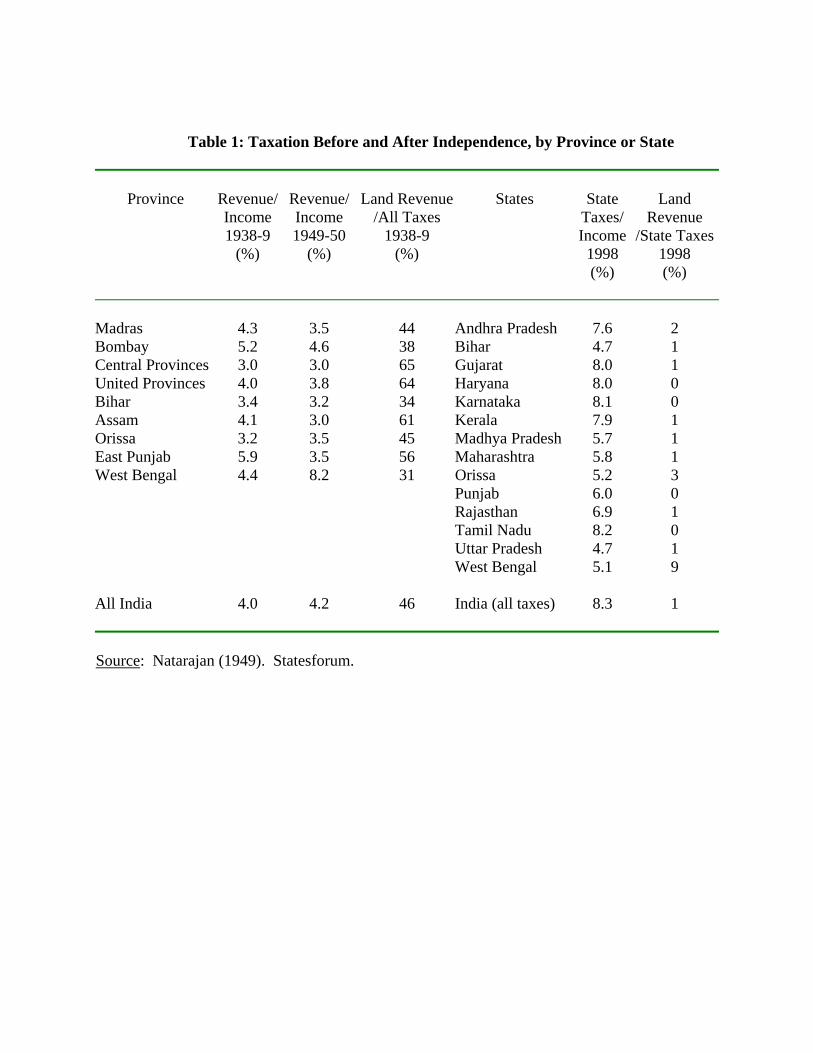
Table 1: Taxation Before and After Independence, by Province or State
Province
Revenue/ Income 1938-9
(%)
Revenue/ Income 1949-50
(%)
Land Revenue
/All Taxes 1938-9
(%)
States
State
Taxes/ Income 1998 (%)
Land
Revenue /State Taxes
1998 (%)
Madras 4.3 3.5 44 Andhra Pradesh 7.6 2 Bombay 5.2 4.6 38 Bihar 4.7 1 Central Provinces 3.0 3.0 65 Gujarat 8.0 1 United Provinces 4.0 3.8 64 Haryana 8.0 0 Bihar 3.4 3.2 34 Karnataka 8.1 0 Assam 4.1 3.0 61 Kerala 7.9 1 Orissa 3.2 3.5 45 Madhya Pradesh 5.7 1 East Punjab 5.9 3.5 56 Maharashtra 5.8 1 West Bengal 4.4 8.2 31 Orissa 5.2 3
Punjab 6.0 0 Rajasthan 6.9 1 Tamil Nadu 8.2 0 Uttar Pradesh 4.7 1 West Bengal 5.1 9 All India
4.0 4.2 46 India (all taxes) 8.3 1
Source: Natarajan (1949). Statesforum.

its gains can be transmitted to the economy as a whole through the migration of capital and labor
within the economy to the successful locality, and through international trade the economy can
specialize production in this sector. In the Industrial Revolution in Britain in 1760-1860 there
was very little productivity growth in the southern half of the country where two thirds of the
population lived in 1760. Most of the productivity growth in the north occurred in textiles. But
through the twin forces of labor migration and international trade the success of Britain in this
one sector was translated into widespread economic growth. By having so much internal
diversity it would seem that India was peculiarly fortunate relative to more homogenous
underdeveloped countries such as its neighbor Bangladesh.
The Sources of Divergence
Why did Indian income per capita decline relative to the advanced economies such as the
USA? The overwhelmingly cause was a decline in the relative efficiency of utilization of
technology in India relative to Britain and the USA. Conventional estimates report that about
one third of the difference in incomes per capita between countries comes from capital
(conventionally measured), and the rest from efficiency (TFP) differences.4 But this assumes
that differences in capital per worker across countries, which are very highly correlated with
differences in income per capita and measured TFP, are exogenous. In a world where capital can
flow between economies capital/worker should be regarded as an endogenous variable, and
would itself be responding to differences in the level of productivity across countries. Thus in
the case of India by the late nineteenth century rates of return on capital were pretty close to
those of England, as table 2 shows. The imperial connection removed all political risk for British
investors.

Table 2: Rates of Return, Britain and India c. 1910
Asset
Rate of Return in Britain
(%)
Rate of Return in India (%)
Agricultural land, 1900-14 2.83 4-6 Industrial Capital, 1900-14 8 7 Railway Equity, 1870-1913 4.3 5.0 Railway Debt, 1870-1913 3.7 3.7 Bank Rate 4.3 5.4
Note: Returns were lower on Indian than British railway bonds because the Indian Government
guaranteed the bonds of the railways as a way of promoting infrastructure investment.
Sources: Edelstein (1982). Goldsmith (1983). Clark (1987, 1998). Wolcott and Clark (1999),
p. 402.
4 See, for example, Easterly and Levine (2000).

Thus suppose the production function was Cobb-Douglas so that
Y = A Kα LβTγ (1)
where T denotes land. Choosing units so that A, K, Y and T are 1 in India, if the rental of capital
were the same across countries, capital per worker in country i, relative to India, would be
(K/L)i = Ai1/(1-α) (T/L)i
γ/(1-α) = (Y/L)i (2)
The amount of capital employed would thus depend on the level of efficiency of the economy.
The more efficient an economy the more capital it would attract, which would have a second
round effect in increasing income per person. Capital per person in this Cobb Douglas case
would be just proportionate to output per person. If capital were exogenously chosen in each
economy then the efficiency (TFP) of other economies relative to India would be
TFPi = Ai = (Y/L)i(K/L)i -α (T/L)i
-γ (3)
But with capital endogenous and rates of return equalized across countries then
(Yi/Li) = (Ai)1/(1-α) (T/L)i -γ/(1-α) (4)
Also the level of efficiency of any economy can be calculated as
Ai = (Y/L)i 1-α (T/L)i
-γ (5)

Table 3: Calculated Relative TFP, USA and Britain (India = 1)
Years
USA TFP
Britain/UK
TFP
1873-79 2.8 3.0 1906-14 3.8 3.8 1947 5.3 4.1 1987* 6.2 4.9 1991* 5.9 4.6 1998* 5.4 4.2
Note: *For these years the assumption that the rate of return to capital was the same in India as
the other countries is suspect because of government regulations in India on foreign investment.

Thus in this case we can calculate relative TFP for the USA and Britain relative to India from
just the relative outputs per capita and the relative amount of land per person. Since the share of
land in national income, γ, has become very small in recent years (4) suggests that the sole
significant cause of differences in income per capita between India and the USA and other
advanced economies is differences in TFP. Table 3 shows the implied TFP of the USA and
Britain relative to India assuming the share of capital in national income was 0.33, and that the
share of land was 0.
After independence in 1947 the Government of India imposed a variety of restrictions on
the free mobility of capital so that the assumption of an equalized rate of return on capital is
suspect. But the proportionality posited above between output per person and capital per person
holds. US output per person was 14.3 times output per person in India in 1992, while capital per
person 17.8 times greater. UK output per person was 10.5 times Indian output, and capital per
person 10.9 times greater (Penn World Tables, version 5.6).
These differences in TFP could have two causes – slow diffusion of Western technology,
or the inability to effectively employ Western technology. We would argue that since the late
nineteenth century the evidence is that technology was able to diffuse rapidly to poor countries,
and that the low TFP of India comes in large part from an inability to effectively employ this
new technology.
If we look at the industry with which we have expertise, cotton textiles, for example, we
see that up to at least the 1940s there is no sign of any Indian lag in the types of machinery
employed compared to the advanced economies. In the early nineteenth century a specialized
machine building sector developed within the Lancashire cotton industry. These machinery
firms, some of which such as Platts were exporting at least 50% of their production as early as

1845-1870, had an important role in exporting textile technology. These capital goods firms
were able to provide a complete "package" of services to prospective foreign entrants to the
textile industry, which included technical information, machinery, construction expertise, and
managers and skilled operatives. By 1913 the six largest machine producers employed over
30,000 workers (Bruland (1989), pp. 5, 6, 34). These firms reduced the risks to foreign
entrepreneurs by such practices as giving them machines on a trail basis, and undertaking to
supply skilled workers to train the local labor force. Similar capital goods exporters developed
in the rail sectors, and later in the U.S. in the boot and shoe industry. The sales records of the
English machine builders have survived along with detailed descriptions of the machines ordered
by each customer. These show that Indian firms were buying Platt machinery of a description
that was very similar to that used in the advanced economies.
Instead the problem that limited the growth of the Indian industry was the low profits
made by cotton mills in India, because of their inability to employ the technology effectively.
These low profits prevented the rapid industrialization of the country under the British despite
India’s great labor cost advantages. Table 4, for example, shows the gross profit rates of
Bombay mills by quinquennia from 1905-9 to 1935-9, as well as the size of the Bombay industry
and the output per worker in Bombay as an index with 1905-9 set at 100. As can be seen profits
were never great, but the industry grew substantially in the era of modest profits up to 1924.
Thereafter, however, profits collapsed (as a result of Japanese competition) and the Bombay
industry soon began to contract. The last column shows what was happening to output per
worker in Japan, where using the same machinery as in India, in both cases purchased from
England, output per worker increased greatly.

Table 4: The Bombay Industry, 1907-1938
Year
Gross profit rate
on fixed capital
Size of the Bombay
Industry (m. spindle-
equivalents)
Output per worker
in Bombay
(Index)
Output per worker
in Japan
(Index)
1905-9 0.09 3.09 100 100 1910-4 0.05 3.43 103 115 1915-9 0.07 3.68 99 135 1920-4 0.08 4.05 94 132 1925-9 -0.00 4.49 91 180 1930-4 0.00 4.40 104 249 1935-9 0.02 3.91 106 281
Notes: Profits and output per worker were calculable only for the mills listed in the Investor’s
India Yearbook.
Source: Wolcott and Clark (1999).

The inefficiency of operation of Indian mills relative to the advanced economies mainly
showed up in terms of very low outputs per worker, rather than in low outputs per machine hour.
Thus output per worker hour using the same technology in spinning cotton yarn in the USA is
many times what it is in India since India entered the factory cotton textile industry. In 1978, for
example, output per worker-hour in cotton spinning was 7.4 times greater in the US than in India
on mills using substantially the same equipment. If there is substantial possibility of capital-
labor substitution then the odd pattern of the same output per spindle-hour but low outputs per
labor-hour in India could still be the result of a generalized managerial inefficiency combined
with a move to substitute labor for capital in Indian mills. But even in elements of the operation
where the substitution possibilities were very limited or non-existent India shows up in textiles as
having low output per worker. Thus in spinning machines are stopped at regular intervals to
remove the output packages in an operation called “doffing.” Since the machines fill at a regular
rate doffing can be scheduled for the machines in rotation and there is no issue of machine
interference from changing the work assignment. Table 5 shows the number of packages doffed
from spinning machines by workers in India, the USA and England in a variety of years from
1907 on (data does not exist for the USA in more recent years because this operation was largely
mechanized). As late as 1990 workers in southern India were completing an average of 230
doffs per hours, and worker productivity at this task in the Gujarat and Maharashtra centers of
the industry was similar. This was less than one quarter of the last recorded average US
performance of 1,000 doffs per hour achieved thirty years earlier in 1959. Yet work study tests
India suggest that, based on performance rates of Indian workers on the tasks doffers in India
complete, a fully employed doffer would complete 863 doffs per hour. Thus compared to both

Table 5: Spindles Doffed per Worker per Hour
Year
USA
England
India
1921 728 - 118a
1944 606 354 124b
1946 770 1949/50 933 570c - 1959 1,000 - - 1969 - 600d - 1978 - - 160e
1990 - - 230
Notes: aBombay City and Island. Calculated from Shirras (1923) on the assumptions that there is one side per ring spinner (170 spindles), that output per spindle-hour averages 0.038 lbs., and that the weight of the doff package is 0.084 lbs (the same as Britain in 1949). bIndia except the Bombay Presidency. cLowest cost mills. dAssumed performance in modernization study. eSouth Indian mills. Doff package assumed to be 0.12 lbs. Sources: Shirras (1923), Cotton Spinning Productivity Team (1951), Ratnam and Rajamanickam (1980), Doraiswamy (1983), SITRA (1990), Textile Council (1969).

US performance in practice, and what Indian workers can complete under work study conditions,
the typical doffer in 1990 actually worked for only about 25% of the their time in the factory.5
Thus the problem of the Indian economy is heavily associated with production
inefficiency. This production inefficiency is observed even when the same methods and
machinery is employed in production in India as in the advanced economies. And this
production inefficiency is associated in particular with an underutilization of the efforts of
workers in the production process.
Regional Income per Capita in India, 1890-1998
While India as a whole has grown poorer relative to the advanced economies since 1873,
there has always been considerable disparity between richer and poorer regions within India, and
this disparity has been growing in recent years. Consideration of regional growth in India is
complicated by the changing boundaries of regions over time. The major administrative break
was caused by the formation of the Republic of India in 1950. The new republic established 14
states and 5 union territories in 1956.6 But new states were created by the subdivision of older
ones in 1960 and 1966, and some union territories have been converted into states so that there
are now 25 states, the last created in 1991. Table 6 shows for the 25 current states their
population in 1991, their principal languages, their rates of urbanization and literacy, and their
income per person in 1991 in rupees of 1990. States were largely based on language groupings.
5 Interestingly the SITRA pamphlet referred to above suggests that the worker assignments would be cost minimizing at only 440 spindle doffs per hour. But it does so on the assumption that (1) any increase in assignment would have to be accompanied by an increase in wages per worker, (2) given the “monotonous and repetitive nature” of doffing it would be too much to expect more of workers, and (3) attempts at higher assignments would result in machine interference. 6 States Reorganization Act of 1956.

Table 6: The Principal Indian States and Territories in 1991
State or Territory
Population 1991 (m.)
Principal Language
Urbanization
(%)
Literacy (%)
Income
/Person (Rs) (1991)
Andhra Pradesh 43.5 Telagu 26 45 4,728 Assam 22.4 Assamese 11 53 4,014 Bihar 86.4 Hindi 13 38 2,655 Delhi* 9.42 Hindi 90 76 10,177 Gujarat 41.3 Gujarati 34 60 5,687 Haryana 16.5 Hindi 22 55 7,502 Himachal Pradesh 5.2 Hindi 9 63 4,790 Jammu & Kashmir 7.7 Urdu 24 27 3,872 Karnataka 45.0 Kannada 31 56 4,696 Kerala 29.1 Malayalam 26 91 4,207 Madhya Pradesh 66.2 Hindi 23 43 4,149 Maharashtra 78.9 Marathi 39 63 7,316 Orissa 31.7 Oriya 13 48 3,077 Punjab 20.3 Punjabi 30 57 8,373 Rajasthan 44.0 Rajasthani 23 39 4,113 Tamil Nadu 55.9 Tamil 34 64 5,047 Uttar Pradesh 139.1 Hindi 20 42 3,516 West Bengal 68.1 Bengali 27 58 4,753 All India 846.3 4,934
Note: *Union Territory. “Others” includes Arunchal Pradesh, Goa, Manipur, Meghalaya, Mizoram, Nagaland, Sikkim, Tripura, and the Union Territory of Pondicherry. Source: Cashin and Sahay (1996).

Table 7: Coefficient of Variation of Income Per Person, India and Europe
Year
India
(19 localities) Wages
Imperial India (10 provinces)
India
(19 states)
India
(14 states)
Non-Communist
Europe (18 Countries)
1890 0.301 - - - 0.23 1914 0.261 - - - 0.21 1938 - 0.293 - - 0.27 1949 - 0.283 - - 0.25 1961 - - 0.22 0.20 0.38 1971 0.352 - - - - 1981 - - - 0.28 - 1991 - - 0.31 0.31 0.21 1998
- - - 0.36 0.17
Notes: 1Carpenters. 2Rural wages only. 3Excluding provinces which later fell in Pakistan. The
earlier Indian data does not control for price level variations, but Bill Collins found that the
national coefficient of variation in real wages across Indian Districts was .337 in 1873-79, and
.355 in 1900-1906 (Collins, (1999), Table 2). Our uncorrected estimates are thus similar in
magnitude.
Luxembourg was omitted from the list of European nations as an outlier.
Sources: Europe. 1890-1950, Prados de la Escosura (2000). 1950-1998, OECD. India GDP.
1938, 1949, Nataraja (1949). 1961, Cashin and Sahay (1996). 1981, 1991, 1998, Statesforum.
India, Wages. 1890, 1914, Datta (1914). 1971, Lal (1988).

There is considerable variation in state real incomes per capita in 1991, even excluding
the union territory of Delhi which has the highest income of all. Incomes in the Punjab in 1991
were 3.2 times those in Bihar. Interestingly the levels of income per capita have actually been
diverging in India since at least 1961, despite the relative uniformity of institutional structure
across states, as shown for example in the small variations in taxes as a share of income revealed
in table 1.7 Table 7, for example, shows the coefficient of variation of various measures of
income per capita across Indian regions from 1890 on. In the earlier colonial period, with no
variation in institutional structure across regions, and improving transport and communications,
income variations were significant and relatively stable. Since Independence the evidence is for
steadily increasing income disparities, both before the economic liberalization of 1991 and since
then. The fortunes of various states have also varied widely. In 1961, for example, West Bengal
was the second richest of the 14 major states, with an income per capita very close to the richest
Maharashtra. By 1998 West Bengal ranked 9th in income per capita, and its income was less
than one half that of Maharashtra.
Figure 2 shows the state real income levels in 1998-9 compared to those of 1991-2 in
rupees of 1993-4. Also shown is the predicted level of income per capita in 1998 based on 1991
when we assume all states’ incomes increased by the same proportion. The figure reveals clearly
that in the 1990s the richest states have been improving their income levels faster than the poorer
7 Aiyar (2001) and Cashin and Sahay (1996) claim to have found convergence in a cross section of Indian states. But they mean by convergence that they can find a regression specification under which the growth rate of income is associated negatively and statistically significantly with the initial level of income, not that actual incomes per capita are becoming less varied. Thus Cashin and Sahay (1996) only find evidence for convergence if they include the initial share of manufacturing in state GDP and the initial share of agriculture in their regressions, and if they divide the periods into decades. Aiyar (2001) finds convergence over the period 1971 to 1995 if he divides the period into 5-year increments, and includes for each period initial literacy and investment. Abler and Das (1998)

Figure 2: Income in 1998-9 as a function of 1991-2 (1993-4 Rupees)
Note: Throughout in the figures we use the following symbols for states: AP, Andhra Pradesh,
B, Bihar, G, Gujarat, H, Haryana, Ka, Karnataka, Ke, Kerala, MP, Madhya Pradesh, Mh,
Maharashtra, O, Orissa, P, Punjab, R, Rajasthan, TN, Tamil Nadu, UP, Uttar Pradesh, WB, West
Bengal. Rajasthan’s income per capita is projected from 1997-8.
Source: Statesforum.
included a measure of investment in their convergence regressions, which covered the entire period, 1961-90, and found no convergence, though they did find a statistically significant effect of investment.

states. Gujarat had a growth rate of income per capita of 7.4%, while Bihar’s was 1.0%. This
despite the facts that the existence of measurement errors in the estimated state GDP per person
in each year will tend to produce an appearance of convergence. In 1991, for example, Bihar,
the poorest of the 14 major states, had a GDP per capita of just 39% of the second richest state
Maharashtra. But by 1998 Bihar’s GDP per capita of only 26% of Maharashtra’s, since income
per capita in Bihar increased by only 7% in these seven years. Indeed relative to the USA the
large northern Indian states of Bihar and Uttar Pradesh, with a combined population in 1998 of
277 million, both saw declining incomes per capita in the 1990s. Three out of the 14 major
states, including these two, had slower growth rates of income per capita in the 1990s than in the
1980s.
India’s experience since the 1960s constrasts sharply with that of western Europe and the
United States. Table 7 shows, for example, for 18 non-communist countries in Europe the
coefficient of variation of incomes back to 1890. 8 While in 1961 these European states showed
much more variation in incomes per capita than did India, by 1998 the position had reversed,
with European states showing dramatic convergence in income levels. The convergence of
incomes per capita across the states of the United States is an oft cited example of a supposedly
general convergence tendency (Barro and Sala-I-Martin, (1991, 1992)). But the experience of
the Indian states, and indeed also of provinces in China, suggests that the convergence witnessed
in Europe and within the United States reveals no general growth law, but a contingent and
accidental feature.9
8 Luxembourg was omitted. By 1999 it had the highest income per capita in the world.

Explaining Income Divergence in India since 1961
Just as the sources of India’s decline in relative income compared to the advanced
economies from 1873 onwards seems unconnected to government policy so the divergence of
income per capita within India again seems largely unconnected with government policy. As
table 1 shows the burden of taxation across Indian states has varied little since independence,
with the wealthier states if anything collecting a larger share of income in taxes. There are more
subtle elements of the regulatory climate in each state that the gross tax burden will not reveal,
but for most important industries, such as textiles, the significant government policy was made at
the Federal level, as with the excise tax on yarn and cloth, and the rights of workers in the mill
sector.10
An investigation of the divergence of incomes in the reform era since 1991 shows no
very promising signs of the effects of state policy. Table 6 shows the effects of some of the
measurable dimensions of state policy such as state taxes as a share of state GDP, public
education expenditure per 100 workers, public capital expenditures per 100 workers, and the
percentage of children enrolled in primary and secondary education. In each case the variable is
included as variable Z in a regression of the form
Growth Rate of GDP/N1991-98 = a + b(GDP/N)1991 + cZ + e (6)
to control for the possible dependence of these Z variables on income per capita. Without any
other variables included the coefficient on (GDP/N)1991 is strongly positive (though significant at
9 China similarly has seen growing income disparities in the years 1978-1998. Income per capita in Guangdong in 1998 was nearly three times that of Quinghai, even though Guangdong’s per capita income slightly lagged that of Quinghai in 1978. Démurger (2001).

Table 8: State Growth and State Policy Measures, 1991-1998 Version
Adjusted R-squared
Variable
Estimated Coefficient
Standard Error
p-value
1. 0.189 Log GDP/N, 1991
2.961 1.474 0.068
2. 0.380 Log GDP/N 1991 0.042 1.867 0.983 Taxes as a Share of state GDP,
1991 (%)
0.654 0.302 0.053
3. 0.233 Log GDP/N 1991 1.059 2.054 0.616 Public Education Expenditure
per 100 workers, 1991 0.015 0.012 0.222
4. 0.147 Log GDP/N 1991 2.604 1.641 0.135 Public Capital Expenditures per
100 workers, 1991 0.006 0.010 0.540
6. 0.436 Log GDP/N, 1991 1.379 1.384 0.340 % Enrolled Primary School,
1981
0.113 0.045 0.029
7. 0.146 Log GDP/N 1991 2.446 1.722 0.184 % Enrolled Secondary
School, 1981
0.049 0.078 0.544
8. 0.431 Log GDP/N 1991 6.716 1.958 0.006 Phones per 100 workers, 1985 -1.906 0.771 0.031
10. 0.123 Log GDP/N 1991 2.923 1.539 0.084 Km. Roads per 100 workers,
1985
0.403 1.345 0.770
Sources: See Appendix Table 1.
10 Thus Misra, in his 1993 book on government policy and the textile sector, has no discussion of any effects of different state policies with regard to textiles (Misra (1993)).

only the 10% level). As can be seen if state taxes as a share of income are included then they are
a much better predictor of growth than the current level of income. The association is that higher
state tax levels in 1991 are associated with faster growth. But if we look at what the states might
do with this revenue to foster income growth the picture is less clear. Both education
expenditures per 100 workers in 1991 and capital expenditures per 100 workers show little sign
of connection with economic growth. The percentage of children enrolled in primary school in
1981 does show a very strong connection with economic growth. But this is a variable only
partially under the control of state governments. And before we get two excited about the
possibilities in fostering economic growth through increased expenditures on education, notice
that the percentage of children enrolled in secondary education in 1981 is not at all a predictor of
growth in the 1990s.
We have two other measures of the states potential success in developing infrastructure,
the number of phones per 100 workers in 1985 and the number of km of roads per 100 workers
in 1985. Neither of these suggests much role for state actions. Phones per worker are
statistically significantly associated with economic growth once we control for initial income.
But the association is negative. And the amount of road infrastructure shows no connection.
Thus if state policy was responsible for the divergence of incomes after 1991 it had to be through
some very subtle measures.
Because the two high income states in 1991 which did not perform so well were Punjab
and Haryana, which were still fairly agricultural and rural, it is possible to predict the growth
rates in the 1990s fairly successfully using measures such as the urbanization rate in 1991 or the
manufacturing share of output in 1991. Figure 3, for example, shows the income growth rates as
a function of the urbanization rates in 1991. But this offers us little insight into the nature of the

Figure 3: Income Growth Rates 1991-8 and Urbanization Rates 1991
Source: Statesforum. Cashin and Sahay (1996).

growth process. The internal variation in economic performance within India seems mainly to
suggest that the role of institutional variations, the kind of things that economists can suggest
advice on, must be limited.
The Employment Relationship
We see above that the obvious correlates that economists have focused on in recent years
to explain differences in income growth rates across economies are of little help in explaining the
movement of income per capita across states in post independence India. What we are
desperately lacking is any kind of hypotheses that would explain the facts of India’s peculiar
economic path in the last 150 years. These facts are as follows.
1. A widening of the economic gap between India and the advanced economies from at
least 1873-1980 on, and probably from as early as 1800.11
2. A de-industrialization of India in response to the industrialization of the advanced
economies, even in the period of free trade. Thus by 1912 India was largely a raw material
exporter. Why, at least in the era of free trade up till 1914 did India not only get poorer relative
to the advanced economies, but also develop a comparative advantage in agriculture?
3. Wide differences in performance by different regions within the same institutional
structures both under the British and after independence.
4. Low levels of performance by workers within India, but high levels of performance
when these workers relocate to other economies such as Britain and the USA. Further no
11 See Williamson quote.

indication that workers in India in such industries as textiles have any less aptitude than those in
the USA in terms of the times taken to perform standard tasks.
The hypothesis we suggest, and it is a speculative one, is the following. The
disadvantage India has relative to the advanced economies is in the employment relationship.
This, to sound almost Marxist, is where a worker sells their labor power for a set time to an
employer. The Industrial Revolution in the West saw not only the development of new
technology, but a greater reliance on the employment relationship as a way of producing output.
In the pre-industrial period most industrial workers were instead sub-contractors. They sold
output to employers in an arms length relationship. The arrival of the steam powered factories in
the 1770s also brought with it a new employment concept, “factory discipline”. Under this new
mode of employment the employer demanded regularity, punctuality, and sobriety from their
employees as opposed to preferring to pay by results. The Industrial Revolution also brought a
greater division of labor within production processes. Each employee specialized more on some
element of the process, and there was also a complex hierarchy of employees supervising
employees.12
The employment relationship, as those who have participated in it all know, is a peculiar
one. In particular the fulfillment of the bargain to labor in exchange for wages is difficult to
monitor. Workers vary in natural abilities, there are uncertain links between inputs and outputs,
and it is often too costly or technically impossible to measure individual outputs. Economists
traditionally think of the employment relationship as being sustained by monitoring and
incentives between rational self-interested workers and employers. But the reality is that an at
least equally important element is the complex human interplay between workers and bosses and
workers and workers involving gift exchanges, pride and notions of fairness. As Akerlof (1982)

and others have stressed, workers give gifts to employers of more effort than they need to avoid
termination, and employers in return give gifts of higher wages than are needed to retain
workers. Economists are always tempted to try to reduce these arrangements to self-enforcing
equilibria between completely rational self-interested agents. Such a reduction would imply that
there can be no difference in the way the employment relationship works between different
countries, unless of course multiple equilibria are possible. Differences in relative prices and
technology may influence the amount of monitoring employers engage in and the amount of
“cheating” workers engage in, but otherwise the employment relationship will be structured
similarly across economies and will generate the same results.
But such a reductionism seems doomed to failure in capturing the nature of the exchange.
Thus, for example, anyone who has purchased services in modern America knows that workers
often give gifts to customers that hurt the interests of their firms. In this case there is no
conceivable benefit to workers. The relationship that will be sustained between employers and
workers depends not just on a rational calculus between self interested agents on the amount of
effort to offer, and the amount of monitoring to engage in, but on the general attitude to gift
giving. Here in America we live in the gift giving society. In most interactions we forbear to
take full advantage of opportunism – we gift the other party with more than we need do, and we
do it without any benefit to ourselves. In part we do this because we have in turn ourselves been
the recipients of many gifts. That is the non-rational calculator element. One case is letting a
person into your lane on a congested highway. There is a cost, you are slowed down slightly,
and no conceivable benefit. But others have done the same for you. Another case is writing
anonymous letters of recommendation for students. This gift giving exchange is sustained in
part by being the recipient of many gifts in turn. It is an equilibrium, but not in the sense
12 See Clark (1994).

understood by economists. We receive from one and we give to another. Mutual gift giving
thus constitutes a social equilibrium. It is self-reinforcing. Its breakdown is also self reinforcing.
Various intermediate equilibria are also possible.
Suppose, however, that the employment relationship works well only in an environment
of mutual gift giving. The unobservabilities in any employment relationship are such that only
when the employed forbear from taking advantage of the unobservability of outcomes will the
relationship work well. Suppose also that in India the cultural equilibrium is for employment not
to constitute the mutual exchange of gifts. Workers expect all other workers to take advantage of
opportunities to shirk, and they adjust their own behavior accordingly. In this case technologies
that rely for their implementation on the employment relationship will be handicapped.
Employees will provide little for their wage. They will be protected by the knowledge that any
potential replacements will provide little also. If all around you give nothing to the employer
then why should you give? Thus we can have several possible employment regimes. One where
most workers voluntarily do more than they have to, and another where all workers act
opportunistically. Since the mutual gift giving is sustained by observing that others do the same
and by receiving gifts yourself subtle changes in behavior can lead to a move to a very different
equilibrium. Workers moving from one environment to another will change their behavior.
Our idea then would be that Indian employers extract little of the labor power they pay
for from employees because of employee’s unwillingness to give voluntarily what is costly to
monitor. The opportunism displayed within the complex hierarchy of employees in modern
production enterprises defeats them.
What would be empirical implications of this hypothesis that we could test? The first
would be that if poor performance by labor in India attaches just to the employment relationship,

then we should observe an adaptation by the economy to avoid this relationship in favor of self-
employment and family employment where possible. India has seen an extraordinary
maintenance in the textile weaving sector, for example, of handlooms. By the 1830s in England
handloom weaving of cottons was largely superceded by power looms in factories, even though
the wages of handloom workers were only about half those of factory workers.13 Yet 170 years
later the handloom sector in India is still very large, particularly in cottons. Indeed the output of
the handloom sector has grown steadily since 1900 when statistics were first gathered. In 1997,
as table 9 shows, output of woven cloth from handlooms in India was about 10 times as great as
in 1900. In 1997-8 25% of cloth production in India was still from handlooms.
Cloth in India is in fact produced in three ways. The mill sector, consisting of large
powerloom plants as in the USA, the handloom sector costing of looms in houses and
workshops, and the “powerloom” sector, consisting of workshops of 1-50 powerlooms outside
the formal regulation of the mill sector. The survival of the handloom industry in India is often
attributed to government protection. Since independence the government has levied excise taxes
on mill output while keeping the handloom sector tax-free. Thus even in 1997-8 most fabrics
paid an excise duty of 10-20%, but handloom cloth was still exempted. However, the informal
13 See Bythell (1969).

Table 9: Cloth Production in India by Sector, 1997-8 (meters2)
Year
Mill Production
Decentralized Powerloom Production
Decentralized
Handloom Production
1900-3 483 0 793 1936-9 3,630 0 1,420 1951 3,740 - - 1973 4,299 - - 1980-1 4,533 4,802 3,109 1997-8 1,948 20,951 7,603
Sources: Office of the Textile Commissioner (1997, 1998). Mazumdar (1984), pp. 7, 36.

“powerloom” sector has largely avoided paying these excise taxes.14 So the tax advantages
mainly serve to explain why smaller powerloom operations could out compete large mills. They
do not explain why handlooms can still compete against untaxed powerloom operations.
Powerlooms produce 2.5 times the amount of output per hour as handlooms, and one weaver
should be able to operate between 4 and 8 powerlooms at a time, based on labor requirements in
Britain and the USA in circa 1900. Day wages per worker in the handloom and powerloom
sectors are about the same, so this implies that powerloom weaving costs per meter of cloth
should be 5-10% of handloom labor costs. Since capital costs for powerlooms per meter are
estimated to be only about 20% higher than for handlooms interest rates would have to be
extraordinarily high before handlooms had any cost advantage. But in practice powerlooms in
India require much more labor even than machine powered looms in England in the nineteenth
century. Powerloom weavers typically supervise only 1.5 looms each (Mazumdar (1984), p. 93).
This drastically reduces the labor cost advantages of the power loom. The high levels of staffing
of power looms might be explained by the very low wages of the operatives, but Indian wages
now are as high or higher than those in England in the 1830s when a more primitive powerloom
easily swept aside the competition of handlooms. The key issue here is that because of the
capital requirements powerlooms are operated with hired labor, while handlooms are placed in
the homes of the workers, and the work is paid for on a piece rate basis.
Similarly if there is anything to the idea that the Indian economy works poorly because of
a difficulty in operating the employment relationship then agriculture in India should tend to be
structured differently, with more use of land renting and less of wage labor than in European
agriculture at a comparable state of mechanization. The second implication would be that
employment relations would be structured differently. If the relationship works because of
14 See Misra (1993), pp. 89-119.

mutual gift giving then there is an incentive to engage in repeated interactions with the same
worker. Employers will prefer to hire the same workers even where there is no learning specific
to the job since then it is easier to establish relationships based on mutual gifts. Employers will
avoid casual labor markets where encounters between the same worker and employer would be
infrequent. Thus we see in agricultural labor markets in pre-industrial England a tendency for
workers to be hired year round by the same employers, and to work for the same employer year
after year. Wages were finely calibrated to the individual worker. In modern rural labor markets
in India, by contrast, workers are typically hired by employers on a casual, daily basis, with little
sign of preference for the same workers by employers. Wage rates paid tend to be standardized,
with little adjustment to individual productivities. Seemingly there is little to be gained by
connection with individual workers.15
As noted above this is a somewhat inchoate hypothesis. It is not at all clear to us if it is
consistent with the details of Indian experience. But it would allow for differences in worker
productivity within the different States that constitute India as created by different social
equilibria with regard to gift giving behavior by workers. And it would also imply that if an
individual worker is transferred from one social setting to another their behavior could change
accordingly. Further it would also explain the widening gap between India and the USA and
other Western Economies from 1873 to the 1980s as the result of the increasing importance of
the employment relationship in modern production systems.
15 See Datt (1996).

Policy Implications
We reach two conclusions above. First that government policy has had little impact on
output per capita in India since 1873 because of the importance of differences in the efficiency of
use of technology in explaining income disparities in general. And second that there has been a
growing regional disparity in incomes per capita within India since at least 1961. In these
circumstances what can the government do to foster growth, and in particular to foster growth in
states like Bihar and Uttar Pradesh which have seen little impact even from the more rapid
growth that began in the 1980s? Within both the USA and Europe movement of people from
low income regions to high income regions has been an important force in increasing overall
economic growth rates. But within India there has been little movement of people towards the
higher income states despite the very large disparities in income that have emerged in the 1990s.
Figure 4 shows the estimated net migration rate per year for the 14 major Indian states from 1991
to 2001 as a percentage of 1991 population as a function of state domestic income per capita in
1998. The net migration rate was estimated from the difference between actual populations in
2001 and those projected from populations in 1991 and state birth and death rates. With the
notable exception of Bihar the states with high incomes in 1998 were clearly net recipients of
migrants, while those with low incomes were net losers of people. But migration rates were very
modest compared to the changes in population occurring through natural increase. Maharashtra,
for example, now the richest Indian state had a net gain of only 0.44% of the population in each
year. But overall population growth in Maharashtra was about 2% per year, so that migration
was a small factor in population change. Similarly outmigration from desperately poor Uttar
Pradesh was estimated at only –0.07% per year, compared to a natural rate of population increase
of 2.8% per year.

Figure 4: Estimated Net Migration per Year 1991-2001 versus State Income per Capita,
1998
Sources: Census of India.

These migration rates between Indian states, where there is no legal impediment to
migration, are very modest compared even to migration rates across European nations in the
1960s when there were significant legal impediments in many cases, and also language barriers.
Figure 5 shows net annual migration rates for non-communist Europe in 1964-71 compared to
income per capita in 1961. These net migration rates include, however, also migration to the
Americas and Australasia. By 1970 after twenty years of constrained post war migration into
Germany and France about 7% of the workforce was foreign born in each country (Faini et al.
(1999)). Hatton and Williamson estimate that between 1870 and 1913 Europe lost 13% of its
population through emigration to the New World, despite the transoceanic nature of this
migration (Hatton and Williamson (1998)).
Within the USA, where the legal and language barriers do not exist net migration rates
between states are even higher. Figure 6 shows net annual internal migration rates for U.S. states
for the years 1900-1999 compared to average annual pay for those employed in 1997 in dollars.
By comparison the limits of state net migration rates in India in the 1990s are also shown. US
domestic net migration rates are many times greater than those in India, though the comparison
may be influenced by the smaller average size of US states. Interestingly US migration has little
on its face to do with differences in wage income per capita across states. The earnings reported
here, however, make no allowance for differences in living costs across states. Also
international migration into US states is quantitatively important, and many of the high income
states losing internal migrants, such as California, New Jersey and New York, are substantial net
recipients of international migrants. Finally there is a significant component of life-cycle
migration of the elderly in the US to high amenity states for retirement purposes. Barro and Sala-
I-Martin (1991) estimated the relationship between relative state income and in-migration in the

Figure 5: European Net Migration per Year 1964-1971 versus National Income per Capita
1961
Note: A, Austria, B, Belgium, D, Denmark, Fi, Finland, Fr, France, WG, West Germany, Gr,
Greece, Ic, Iceland, Ir, Ireland, It, Italy, Ne, Netherlands, No, Norway, P, Portugal, Sp, Spain,
Sw, Sweden, Sz, Switzerland, UK, United Kingdom
Source: United Nations (1991).

Figure 6: Net Internal Migration Rates, 1990s, US States
Source: U.S., Census Bureau.

1980s controlling for some of these factors. They find that a 10% increase in a state’s per capita
income leads to a 0.26 percentage point increase in net migration per year. That responsiveness
of migration to economic opportunity transferred to India would imply that a state like
Maharashtra with an income per capita in 1998 85% greater than the rest of India would
experience net migration equivalent to 2.2% of its population per year, five times the actual rate
for the 1990s. Bihar equivalently, with 42% of the average income of the rest of India would be
loosing about 1.5% of its population per year at US internal migration rates.16 Had even 1% of
the population of the lowest income states in India, Bihar, Uttar Pradesh and Orissa, moved to
the highest income states in each year in the 1990s the growth rate of income per capita in India
would have been increased by 0.3% per year.17 This is not huge, but it is a more substantial
boost to income growth rates than any other feasible action Indian policy makers might take.
16 These rates are calculated for cases where the income disparities between states are much less than in India. The responsiveness in the US to a change from a 50% income premium to a 60% premium might well be much greater than going from a 10% premium to a 20% premium. 17 Assuming that the migration did not affect per capita incomes in the sending and receiving states. But this in the light of historical evidence seems a reasonable assumption.

Bibliography Official Reports Data on Nominal and Real GDP for 14 of the major Indian states as well as state government capital and regular expenditure and revenue sources can be found at www.statesforum.org. Central Statistical Organisation, Dept. of Statistics, Ministry of Planning, Basic Statistics Relating to the Indian Economy, 1950-51 to 1978-79. Delhi, 1980. Economic Report of the President, 2001. Washington, D.C.: Government Printing Office. Office of the Textile Commissioner, Mumbai. 1997. Compendium of Textile Statistics, 1997. Mumbai, India. Office of the Textile Commissioner, Mumbai. 1998. Basic Textile Statistics for 1997-8. Mumbai, India. Southern India Textile Research Association, Doffing Boy Productivity in Ring Spinning (SITRA Focus, Vol. 8, Sept 1990, No. 3 (Revised 1994)). United Nations, Dept. of International Economic and Social Affairs, Statistical Office. Demographic Yearbook, 1989. New York, 1991. Secondary Aiyar, Shekhar, “Growth Theory and Convergence Across Indian States: A Panel Study,” in
Tim Callen, Patricia Reynolds and Christopher Towe (ed.), India at the Crossroads. Washington, D.C.: International Monetary Fund, 2001.
Akerlof, George A. “Labor Contracts as Partial Gift Exchange” Quarterly Journal of
Economics, Vol. 97, No. 4. (Nov., 1982), pp. 543-569. Balke, Nathan S. and Robert J Gordon, “The Estimation of Prewar Gross National Product:
Methodology and New Evidence,” Journal of Political Economy, vol. 97, no. 1 (Jan 1992), pp. 38-92.
Barro, Robert J. and Xavier Sala-I-Martin, “Convergence across States and Regions,” Brookings
Papers on Economic Activity, v. 1, (1991), pp. 107-182. Barro, Robert J. and Xavier Sala-i-Martin, “Convergence,” Journal of Political Economy, vol.
100, no. 2 (April 1992), pp. 223-251. Bruland, Kristine. British Technology and European Industrialization: The Norwegian Textile
Industry in the mid Nineteenth Century. Cambridge: Cambridge University Press, 1989.

Bythell, Duncan. The handloom weavers: a study in the English cotton industry during the
Industrial Revolution. London, Cambridge University Press, 1969. Cashin, Paul and Sahay, Ratna, “Internal Migration, Center-State Grants, and Economic Growth
in the States of India, IMF Staff Papers, Vol. 43, No. 1 (March 1996), pp. 123-171. Clark, Gregory, "Why Isn't the Whole World Developed? Lessons from the Cotton Mills,"
Journal of Economic History, 47 (March 1987): 141-173. Clark, Gregory. “Factory Discipline,” Journal of Economic History, 54 (March, 1994), 128-163. Clark, Gregory. “Land Hunger: Land as a Commodity and as a Status Good in England, 1500-
1910,” Explorations in Economic History, 35(1) (Jan., 1998), 59-82. Collins, William J., “Labor Mobility, Market Integration, and Wage Convergence in Late 19th
Century India,” Explorations in Economic History, 36, no. 3 (July, 1999), pp. 246-277. Cotton Spinning Productivity Team. Cotton Spinning. London: Anglo-American Council on
Productivity, 1951. Datt, Gaurav. Bargaining power, wages and employment : an analysis of agricultural labor
markets in India. Thousand Oaks, Calif.: Sage Publications, 1996. Datta, Krishna Lal. Report on the enquiry into the rise of prices in India. Calcutta,
Superintendent Government Printing, India, 1914. De Long, J. Bradford. “India Since Independence: An Analytic Growth Narrative.” This
volume, 2001. Démurger, Sylvie. “Infrastructure Development and Economic Growth: An Explanation for
Regional Disparities in China?” Journal of Comparative Economics, 29 (2001): 95-117. Doraiswamy, Indra. "Scope for Increasing Productivity in Spinning Mills," in Resume of Papers,
Twenty Fourth Technological Conference. ATIRA, BTRA, NITRA, and SITRA. 1983. Edelstein, Michael. Overseas investment in the age of high imperialism : the United Kingdom,
1850-1914. New York : Columbia University Press, 1982. Faini, Riccardo, Jaime de Melo and Klaus F. Zimmermann, (ed.), Migration: the Controversies
and the Evidence, Cambridge University Press (1999). Feinstein, C. H.. National income, expenditure and output of the United Kingdom, 1855-1965.
Cambridge: Cambridge University Press, 1972.

Goldsmith, Raymond, The Financial Development of India, 1860-1977. Yale, Yale University Press, 1983.
Hatton, Timothy J. and Jeffrey G. Williamson, The Age of Mass Migration, Oxford University
Press (1998). Heston, Alan. “National Income” in The Cambridge Economic History of India, Volume 2
c.1751–c.1970. Edited by Dharma Kumar, Meghnad Desai. Cambridge, Cambridge University Press, 1983.
Hurd, John, “Railways,” in The Cambridge Economic History of India, (ed.) Dharma Kumar and
Meghnad Desai, Delhi: Cambridge Univerversity Press, 1982., pp. 737-761. Lal, Deepak, “Trends in Real Wages in Rural India: 1880-1980,” in (ed.)T.N. Srinivasan and
Pranab K. Bardhan, Rural Poverty in South Asia, New York: Columbia University Press (1988), pp. 265-293.
Mazumdar, Dipak. “The Issue of Small versus Large in the Indian Textile Industry: An
Analytical and Historical Survey,” World Bank Staff Working Papers, #645. The World Bank, Washington, D. C., 1984.
Misra, Sanjiv. India’s Textile Sector: A Policy Analysis. Sage Publications, New Delhi, 1993. Natarajan, B. An Essay on National Income and Expenditure in India. Madras: Economic
Advisor to the Government of Madras, 1949. Ratnam, T. V. and R. Rajamanickam (1980), "Productivity in Spinning: Growth and Prospects," in
Resume of Papers, Twenty First Technological Conference. ATIRA, BTRA, and SITRA. Prados de la Escosura, Leandro. “International Comparisons of Real Product, 1820-1990: An
Alternative Data Set.” Explorations in Economic History, 37 (1): 1-41, 2000. Shirras, G. Findlay. Report of an Enquiry into the Wages and Hours of Labour in the Cotton Mill
Industry. Labour Office, Government of Bombay: Bombay, 1923. SITRA. “Doffing Boy Productivity in Ring Spinning.” Southern India Textile Research
Association, Focus, Vol. 8, No. 3, September 1990. Robert Summers and Alan Heston (1991), "The Penn World Table (Mark 5): An Expanded Set
of International Comparisons," Quarterly Journal of Economics 106:2 (May), pp. 327-68. Textile Council, Cotton and Allied Textiles. Manchester, 1969. A Social and Economic Atlas of India. Delhi: Oxford University Press, 1987.

Wolcott, Susan and Gregory Clark. “Why Nations Fail: Managerial Decisions and Performance in Indian Cotton Textiles, 1890-1938.” Journal of Economic History, 59(2) (June, 1999): 397-423.

Appendix Table 1. Data Sources used in Regression Analysis
Variable
Source
State GDP per capita, 1991-2 and 1998-9 www.statesforum.org Annual Rate of population Growth, 1961-1991 and 1990-1997
Indian Central Statistical Office, Basic Statistics (1980). www.censusindia.net
Adult Literacy, 1991
www.censusindia.net
% of 5 to 14 year olds enrolled in primary school
A Social and Economic Atlas of India (1987)
% of 10 to 19 year olds enrolled in secondary school
A Social and Economic Atlas of India (1987)
Taxes as a share of state GDP, 1990-98
www.statesforum.org
Public Capital Expenditures per 100 workers, 1990-98a
www.statesforum.org. A Social and Economic Atlas of India (1987)
Education Expenditures per 100 workers, 1990-98a
www.statesforum.org. A Social and Economic Atlas of India (1987)
Phones, Km. Roads and Telephones per 100 workers, 1985
A Social and Economic Atlas of India (1987)
Urbanization, 1961 and 1991 Indian Central Statistical Office, Basic Statistics (1980). www.censusindia.net
aWorkers are defined as those 15 to 59 participating in the labor force.