PRINCETON STUDIES IN INTERNATIONAL FINANCE

No. 76, September 1994

ONE MONEY OR MANY?

ANALYZING THE PROSPECTS FOR MONETARY

UNIFICATION IN VARIOUS PARTS OF THE WORLD

TAMIM BAYOUMI

AND

BARRY EICHENGREEN

INTERNATIONAL FINANCE SECTION

DEPARTMENT OF ECONOMICSPRINCETON UNIVERSITY

PRINCETON, NEW JERSEY

PRINCETON STUDIESIN INTERNATIONAL FINANCE

PRINCETON STUDIES IN INTERNATIONAL FINANCE arepublished by the International Finance Section of theDepartment of Economics of Princeton University. Al-though the Section sponsors the Studies, the authors arefree to develop their topics as they wish. The Sectionwelcomes the submission of manuscripts for publicationin this and its other series. Please see the Notice to Con-tributors at the back of this Study.

The authors of this Study are Tamim Bayoumi andBarry Eichengreen. Tamim Bayoumi is an economist atthe Research Department of the International MonetaryFund and has published a number of articles in the fieldsof international finance and macroeconomics. BarryEichengreen is John L. Simpson Professor of Economicsand Professor of Political Science at the University ofCalifornia at Berkeley. He is, most recently, the author ofInternational Monetary Arrangements for the 21st Century(1994). This is his third contribution to the publicationsof the International Finance Section.

PETER B. KENEN, DirectorInternational Finance Section

PRINCETON STUDIES IN INTERNATIONAL FINANCE

No. 76, September 1994

ONE MONEY OR MANY?

ANALYZING THE PROSPECTS FOR MONETARY

UNIFICATION IN VARIOUS PARTS OF THE WORLD

TAMIM BAYOUMI

AND

BARRY EICHENGREEN

INTERNATIONAL FINANCE SECTION

DEPARTMENT OF ECONOMICSPRINCETON UNIVERSITY

PRINCETON, NEW JERSEY

INTERNATIONAL FINANCE SECTIONEDITORIAL STAFF

Peter B. Kenen, DirectorMargaret B. Riccardi, EditorLillian Spais, Editorial Aide

Lalitha H. Chandra, Subscriptions and Orders

Library of Congress Cataloging-in-Publication Data

Bayoumi, Tamim A.One money or many? : analyzing the prospects for monetary unification in various

parts of the world / Tamim Bayoumi and Barry Eichengreen.p. cm. — (Princeton studies in international finance, ISSN 0081-8070 ; no. 76)Includes bibliographical references.ISBN 0-88165-248-2 (pbk.) : $11.001. Monetary unions. 2. Monetary policy. I. Eichengreen, Barry J. II. Title. III.

Series.HG3894.B39 1994332.4′566—dc20 94-22966

CIP

Copyright © 1994 by International Finance Section, Department of Economics, PrincetonUniversity.

All rights reserved. Except for brief quotations embodied in critical articles and reviews,no part of this publication may be reproduced in any form or by any means, includingphotocopy, without written permission from the publisher.

Printed in the United States of America by Princeton University Printing Services atPrinceton, New Jersey

International Standard Serial Number: 0081-8070International Standard Book Number: 0-88165-248-2Library of Congress Catalog Card Number: 94-22966

CONTENTS

1 INTRODUCTION 1

2 OPTIMUM CURRENCY AREAS 4Nature of Disturbances 4Ease of Response 5Implication for Policy 6

3 METHODOLOGY 8

4 DATA 14

5 ESTIMATION 21

6 ESTIMATION RESULTS 23Correlation of Disturbances 23Correlation of Demand Shocks 25Size of Disturbances 27Speed of Adjustment 27Recapitulation 29

7 UNITED STATES REGIONAL DATA 30

8 CONCLUSIONS 33

REFERENCES 37

FIGURE

1 The Aggregate Supply and Demand Model 9

TABLES

1 Basic Statistics of Different Geographic Regions 15

2 Correlations of Growth across Different GeographicRegions 18

3 Correlations of Inflation across Different GeographicRegions 19

4 Correlations of Supply Disturbances with Changes inTerms of Trade 22

5 Correlations of Supply Disturbances across DifferentGeographic Regions 24

6 Correlations of Demand Disturbances across DifferentGeographic Regions 26

7 Disturbances and Adjustment across DifferentGeographic Regions 28

8 Correlations of Disturbances across Regions in theUnited States 31

9 Regional Disturbances and Adjustment in the United States 32

1 INTRODUCTION

Part of the research for this paper was completed while Tamim Bayoumi was at theBank of England and Barry Eichengreen was at the Federal Reserve Board. Financialsupport for Barry Eichengreen was provided by the Center for German and EuropeanStudies of the University of California at Berkeley. The views expressed in this study aresolely the authors’, however, and do not necessarily represent those of the above institu-tions or of the International Monetary Fund.

Recent years have witnessed a number of developments that have thepotential to transform national and international monetary arrangements.The Maastricht Treaty is an important step toward the adoption of asingle European currency by at least some members of the EuropeanUnion (EU).1 Political disintegration in the former Soviet Union,Yugoslavia, and Czechoslovakia, spelling the end to three existingcurrency unions, is a significant step in the other direction. Looking intothe future, the move toward regionally based free-trade areas in NorthAmerica, East Asia, and South America may eventually prompt policy-makers in these regions, as in Europe, to contemplate the creation ofsingle regional currencies.2

These developments have rekindled interest in the literature onoptimum currency areas initiated by Mundell in 1961. In Mundell’sframework, the gains from monetary unification and a common currencystem from lower transaction costs and the elimination of exchange-ratevariability. Losses come from the inability to pursue independentmonetary policies and to use the exchange rate as an instrument ofadjustment. The magnitude of the losses depends on the incidence ofdisturbances and the speed with which the economy adjusts. If distur-bances and responses are similar across regions, symmetrical policyresponses will suffice, eliminating the need for policy autonomy. Onlyif disturbances are asymmetrically distributed across countries or ifspeeds of adjustment are markedly different will distinctive nationalmacroeconomic policies be needed and the constraints of monetaryunion be a hindrance.

1 Formerly called European Community (EC).2 For a detailed discussion of regional trading arrangements in these areas, see Torre

and Kelly (1992).

1

Disturbances and responses are not, of course, the only factorsinfluencing the choice of international monetary arrangements. Mundell(1961) emphasized the importance of factor mobility for facilitatingadjustment. McKinnon (1963) argued that the gains from unificationwere likely to be an increasing function of the openness of the constitu-ent economies to intraregional trade (because openness magnifies thegains associated with the reductions of the transaction costs). And Kenen(1969) proposed that the diversification of the economy should be usedto assess the appropriateness of a currency area, arguing that highlydiversified economies are less likely to experience the sort of asymmetricshocks that independent exchange rates are useful for offsetting.

Several recent studies investigate the incidence of disturbances as away of analyzing the suitability of different groups of nations formonetary union. Many of these studies focus on Europe, where the issuehas particular immediacy, and some compare the variability of relativeprices in the EU with those in existing monetary unions like the UnitedStates and Canada (Poloz, 1990; Eichengreen, 1992; De Grauwe andVanhaverbeke, 1993). A limitation of this approach is that the movementof relative prices conflates the effects of disturbances and responses; itis not possible to identify the relevant structural parameters on the basisof the behavior of such semi-reduced-form variables. Some other studiesconsider the behavior of output itself, attempting to distinguish commonfrom idiosyncratic national shocks (Cohen and Wyplosz, 1989; Weber,1991). These studies compute sums and differences in output move-ments for groups of European countries, interpreting the sums assymmetric disturbances and the differences as asymmetric disturbances.The problem with this approach is that output movements are not thesame as shocks; they, too, conflate information on disturbances andresponses. This strategy also fails to distinguish between disturbancesemanating from different sources, such as impulses to demand relatedto the conduct of monetary and fiscal policies as against shifts in supplyassociated with the shocks to the real economy.

The present study uses a structural vector-autoregression approachdeveloped by Blanchard and Quah (1989) to identify aggregate supplyand demand disturbances and to distinguish them from subsequentresponses.3 These measures can be used to identify groups of countries

3 The authors used this approach previously in a series of related papers to analyzeEconomic and Monetary Union (EMU), the possible extension of EMU to the EuropeanFree Trade Association (EFTA) countries, and the North American Free Trade Agreement(NAFTA), respectively (Bayoumi and Eichengreen, 1993, 1994a, 1995).

2

suited for monetary union. The estimated disturbances point to moreclear-cut groupings than the time series on output and the prices fromwhich they are derived. Vector autoregression identifies three sets ofcountries that, on the basis of their macroeconomic disturbances andresponses, are plausible candidates for monetary unification: a North-ern European group comprised of Germany and a subset of otherpotential participants in EMU (Austria, Belgium, Denmark, France, theNetherlands, and perhaps Switzerland); a Northeast Asian bloc (Japan,Korea, and Taiwan); and a Southeast Asian area (Hong Kong, Indonesia,Malaysia, Singapore, and possibly Thailand). Notably absent from thislist are countries in either North or South America.

To provide a context in which to interpret our results, Chapter 2presents a selective survey of the literature on optimum currency areas.Chapters 3 and 4 describe the methodology we used to distinguishdisturbances and adjustment dynamics and the data employed in theanalysis. Chapters 5 and 6 report our estimates and discuss theirimplications. Chapter 7 presents, for comparison, results using regionaldata for the United States, an existing monetary union. Chapter 8 con-cludes the study.

3

2 OPTIMUM CURRENCY AREAS

This chapter selectively surveys the literature on optimum currencyareas and highlights aspects and ambiguities of that inquiry relevant tothe analysis presented below. For more comprehensive surveys, thereader may consult Ishiyama (1975) or Tavlas (1992).

Mundell, in his seminal contribution, emphasized two criteriapertinent to deciding whether to abandon policy autonomy for amonetary union: the nature of disturbances and the ease of response.We consider them in turn.

Nature of Disturbances

If two regions experience the same disturbances, they will presumablyfavor the same policy responses.1 Abandoning policy autonomy formonetary unification will then entail relatively little cost. It is curiousthat the magnitude of disturbances, as opposed to their correlation, hasreceived little attention in the literature. Consider a set of disturbancesthat are negatively correlated across a pair of countries. If those distur-bances are of negligible size, the two countries may still incur onlyminor costs from forsaking policy autonomy because output, unemploy-ment and other relevant variables will barely be disturbed from theirequilibrium levels. Clearly, discussions of monetary unification focusingon the nature of disturbances should consider their size as well as theircross-country correlation.

Subsequent to Mundell, the literature has followed Kenen (1969) inlinking structural characteristics of economies—and, in particular, thesectoral composition of production—to the characteristics of shocks.This literature suggests that economies sharing the same industries arelikely to experience similar aggregate disturbances insofar as economy-wide disturbances are the aggregates of industry-specific shocks. Ifdisturbances are imperfectly correlated across industries, diversifiedeconomies may experience smaller aggregate disturbances than willhighly specialized economies. In particular, if two economies specializein sectors that respectively produce and use primary products, there is

1 Strictly speaking, this assumes that preferences in the two countries are the same.Corden (1972) suggests that differences in preferences across countries can also obstructmovement toward monetary union.

4

good reason to anticipate that the disturbances they experience will benegatively correlated.

Ease of Response

If market mechanisms adjust smoothly and restore equilibrium rapidly,asymmetric disturbances need not imply significant costs for entitiesdenied the option of an independent policy response. Even largeshocks that displace macroeconomic variables from normal levels willhave relatively small costs if the initial equilibrium is restored quickly.

Mundell focused on labor mobility as an adjustment mechanism. Ifasymmetric shocks raising unemployment in one region relative toanother elicit labor flows from the former to the latter, unemploymentmay return to normal levels before significant costs have been incurredeven if the authorities lack policy instruments to expedite adjustment.Blanchard and Katz (1992) have recently affirmed the importance of thismechanism in the United States. Interregional migration contributesmore to internal adjustment in the United States than do changes ineither relative wages or labor-force participation rates. It is clear fromthe work of Blanchard and Katz, however, that migration is but one ofseveral channels through which adjustment to asymmetric shocks canoccur. Equilibrium is also restored through adjustments in relativewages (upward in regions experiencing positive shocks, downward inothers), by the changes in labor-force participation induced by thesewage changes, and by capital mobility into those regions experiencingtemporary negative disturbances. Blanchard and Katz conclude, however,that, for the United States, the Mundellian assumption that labormobility is the principal channel for adjustment is broadly consistentwith the facts. They also identify differences across regions in theimportance of the different adjustment mechanisms. In the U.S.manufacturing belt, for example, relatively little adjustment occursthrough changes in relative wages.

Whether potential monetary unions in other parts of the worlddisplay comparable labor mobility is questionable. The Organisation forEconomic Co-operation and Development (OECD, 1987) providestabulations indicating that French and German workers are only a thirdas likely to move between départements and lander as Americans are tomove between states. According to migration equations reported inEichengreen (1993), the elasticity of interregional migratory flows withrespect to internal wage and unemployment differentials is smaller inGreat Britain and Italy than in the United States. Guest workers fromTurkey and other sources outside the EU may be more mobile and

5

responsive to changes in economic conditions, but, in many countries,their impact on destination labor markets is limited to unskilled jobsand the informal sector. Goto and Hamada (1994) point to the extentof labor mobility in Asia, where countries like Singapore have a largershare of immigrants in their labor force than has any industrial countrybut Switzerland. Other countries like Japan and South Korea, however,are less accommodating of guest workers.

Implication for Policy

The implication for policy is that countries experiencing large asymmet-ric disturbances are poor candidates for forming a monetary union,because these are the countries where policy autonomy has the greatestutility. Indeed, this is the implication we use in this paper to interpretour empirical results. Before proceeding, however, it is worth notingseveral qualifications.

First, even if countries experience large, asymmetric disturbances, itneed not follow that policy autonomy is useful for facilitating adjust-ment. If money is neutral, it will not help to offset disturbances tooutput. Most of the recent literature on monetary policy, however,though written by authors approaching the question from very differentperspectives, does support the view that monetary initiatives affectrelative prices and quantities (for example, Romer and Romer, 1989;Eichenbaum and Evans, 1993). In models with coordination failure,nominal contracting, and other sources of inertia, monetary policy canspeed adjustment whether the disturbance in question is a supply shockthat permanently shifts the long-run equilibrium or a demand shock thattemporarily displaces output and prices from invariant steady-state levels.

Second, even countries that value policy autonomy may be willing toabandon monetary independence if they retain other flexible policyinstruments, of which fiscal policy is the obvious candidate. In monetaryunions like the United States, state and local governments run budgetdeficits in periods of recession and accumulate nonnegligible debts. In1990, the ratio of state debt to gross state product averaged 2.4 per-cent.2 In practice, the high mobility of capital and labor in a monetaryunion constrains the fiscal flexibility of constituent jurisdictions. Ifmobile factors of production are able to flee the taxes needed to serviceheavy debt burdens, governments may find themselves unable to financebudget deficits by borrowing in capital markets cognizant of this

2 Many states impose statutory and constitutional limits on their ability to borrow; seebelow and in Bayoumi and Eichengreen (1994b).

6

constraint on the authorities’ capacity to tax. Bayoumi and Eichengreen(1994b) estimate that state governments in the United States, whichoperate in an environment of high factor mobility, find themselvesrationed out of the capital market when their debt-to-income ratiosapproach 9 percent. In addition, worries that participants in a monetaryunion will free-ride by issuing debt in excess of their ability to serviceit, forcing other members to bail out them out, has led the architects ofthe CFA franc zone and the EU’s prospective monetary union to adoptstatutes designed to limit the fiscal autonomy of constituent jurisdictions.Finally, there is the fact that, for political reasons, fiscal policy is lesseasily adapted than monetary policy to changing economic conditions.For all these reasons, fiscal policy is likely to be an imperfect substitutefor the abandoned monetary instrument.

A third qualification is that policymakers may systematically misusepolicy rather than employ it to facilitate adjustment. For countries thatsuccumb repeatedly to high inflation, for example, it is hard to arguethat forsaking monetary-policy autonomy is costly. One interpretation ofasymmetrically distributed aggregate demand shocks is that the countriesconcerned are poor candidates for monetary union, because policymak-ers can use demand-management instruments to offset demand shocksemanating from other sources. But, if domestic policy itself is the sourceof the disturbances, monetary unification with a group of countries lesssusceptible to such pressures may imply a welfare improvement.

A fourth and final qualification is that the nature of disturbancesacross a group of countries may be correlated with other characteristicsthat also affect their suitability for participation in a monetary union.Take, for instance, Kenen’s point that a high degree of specialization inproduction is likely to be associated with asymmetric shocks andtherefore with floating exchange rates between separate currencies. Ahigh degree of specialization also implies that floating exchange ratesmay be very disruptive of living standards. Fixing the value of thenational currency in terms of a country’s dominant export commodity—this being the implication of adopting a floating rate—will subjecthouseholds to fluctuations in their purchasing power. These householdsmay prefer that the government insure them against purchasing-powerfluctuations by stabilizing the value of the currency in terms of somebroader aggregation of goods, that is, by fixing the exchange rate or byjoining a monetary union. In practice, a high degree of specializationappears to be one of the strongest empirical correlates of the decisionto peg the exchange rate (see, for example, the evidence provided byHonkapohja and Pikkarainen, 1992).

7

3 METHODOLOGY

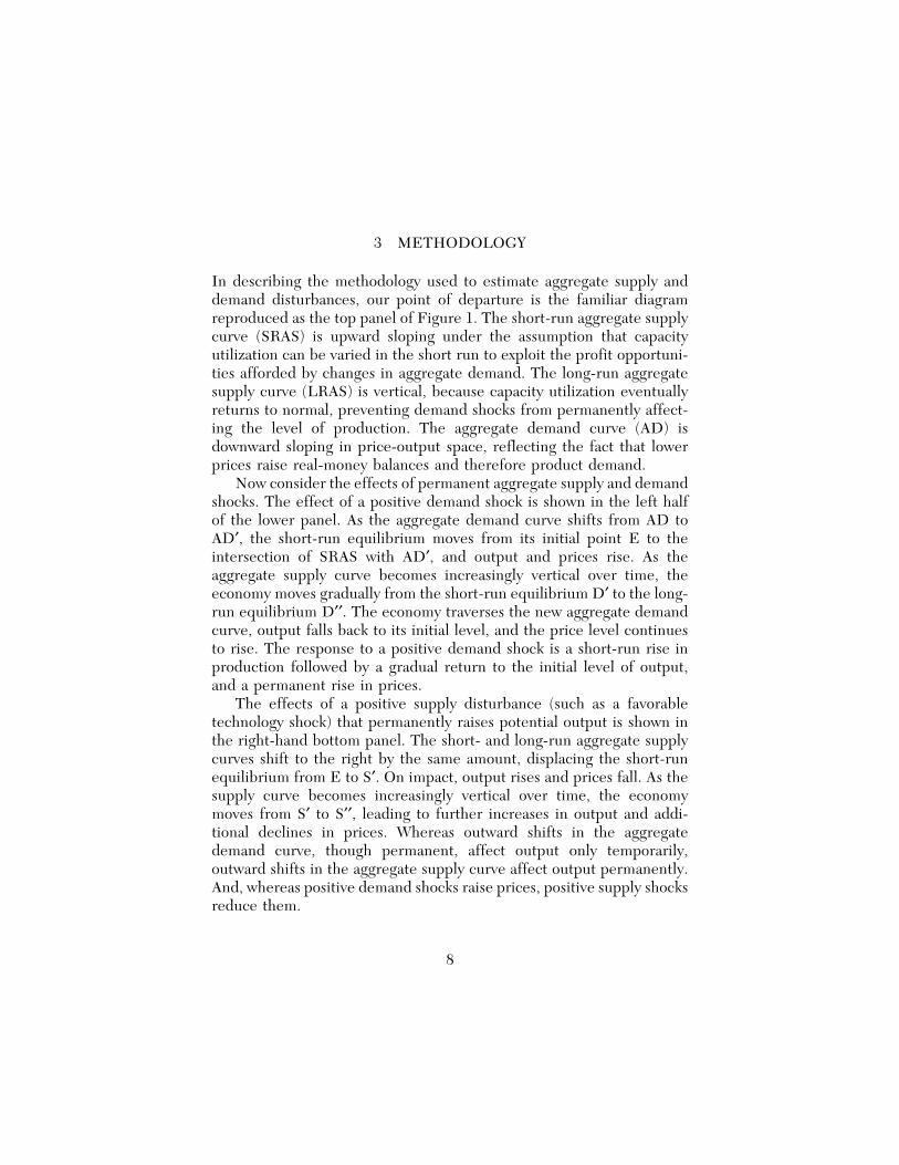
In describing the methodology used to estimate aggregate supply anddemand disturbances, our point of departure is the familiar diagramreproduced as the top panel of Figure 1. The short-run aggregate supplycurve (SRAS) is upward sloping under the assumption that capacityutilization can be varied in the short run to exploit the profit opportuni-ties afforded by changes in aggregate demand. The long-run aggregatesupply curve (LRAS) is vertical, because capacity utilization eventuallyreturns to normal, preventing demand shocks from permanently affect-ing the level of production. The aggregate demand curve (AD) isdownward sloping in price-output space, reflecting the fact that lowerprices raise real-money balances and therefore product demand.

Now consider the effects of permanent aggregate supply and demandshocks. The effect of a positive demand shock is shown in the left halfof the lower panel. As the aggregate demand curve shifts from AD toAD′, the short-run equilibrium moves from its initial point E to theintersection of SRAS with AD′, and output and prices rise. As theaggregate supply curve becomes increasingly vertical over time, theeconomy moves gradually from the short-run equilibrium D′ to the long-run equilibrium D′′. The economy traverses the new aggregate demandcurve, output falls back to its initial level, and the price level continuesto rise. The response to a positive demand shock is a short-run rise inproduction followed by a gradual return to the initial level of output,and a permanent rise in prices.

The effects of a positive supply disturbance (such as a favorabletechnology shock) that permanently raises potential output is shown inthe right-hand bottom panel. The short- and long-run aggregate supplycurves shift to the right by the same amount, displacing the short-runequilibrium from E to S′. On impact, output rises and prices fall. As thesupply curve becomes increasingly vertical over time, the economymoves from S′ to S′′, leading to further increases in output and addi-tional declines in prices. Whereas outward shifts in the aggregatedemand curve, though permanent, affect output only temporarily,outward shifts in the aggregate supply curve affect output permanently.And, whereas positive demand shocks raise prices, positive supply shocksreduce them.

8

External as well as internal disturbances are readily incorporated intothe framework of aggregate supply and demand. Consider, for example,a rise in oil prices. For oil-importing countries, such a disturbanceshould be treated first and foremost as a supply shock. The change inthe relative price of inputs lowers the value of the existing capital stock,reducing the equilibrium level of output. But there are also negativerepercussions on demand owing to the adverse movement in the termsof trade. This, however, is not likely to be large in the case of oil-importing countries, because the proportion of total demand that isassociated with oil consumption is relatively small. The impact onaggregate demand is therefore likely to be swamped by the macro-economic policy response to the oil-price shock.

The same need not be true for countries where output is dominatedby production of oil (or other raw materials). In those countries, achange in relative prices is likely to show up as both an aggregate supplydisturbance and an aggregate demand disturbance. A rise in oil pricesis likely to affect Indonesia, for example, both by raising the underlyinglevel of output through the increased incentive to produce oil and byboosting aggregate demand through the favorable impact of the termsof trade on real incomes. Hence, for producers of oil, it may be difficultto distinguish between the aggregate supply and demand disturbancescaused by a change in oil prices.

We estimate our model using a procedure proposed by Blanchardand Quah (1989) for distinguishing temporary from permanent shocksto a pair of time-series variables; it was extended to the present case byBayoumi (1992). Consider a system in which the true model can berepresented by an infinite moving average of a (vector) of variables Xt

and an equal number of shocks εt. Using the lag operator L, this can bewritten as

where the matrices Ai represent the impulse response functions of the

(1)X

tA0 ε

tA1 ε

t 1 A2 εt 2 A3 ε

t 3 ...∞

i 0

L i Aiε

t,

shocks to the elements of X.Specifically, let Xt be made up of change in output and the change

in prices, and let εt be supply and demand shocks. Then, the modelbecomes

10

where yt and pt represent the logarithm of output and prices, a11i

(2)

∆yt

∆pt

∞

i 0

L i

a11ia12i

a21ia22i

εdt

εst

,

represents element a11 in matrix Ai, and εdt and εst are independentsupply and demand shocks. The two shocks will be independent if theyhave separate causes, such as shifts in macroeconomic policy in the caseof aggregate demand disturbances and technological innovations in thecase of aggregate supply disturbances. If, however, the same underlyingdisturbance causes movements in both cases—for example, a change incommodity prices for a commodity producer—this identification willbreak down. The estimated aggregate supply disturbance in this case willincorporate the associated effect on aggregate demand (see furtherdiscussion below).

This framework implies that, although supply shocks have permanenteffects on the level of output, demand shocks have only temporaryeffects (though both have permanent effects on the level of prices).Because output is written in first-difference form, the cumulative effectof demand shocks on the change in output (∆yt) must be zero. Thisimplies the restriction

The model defined by equations (2) and (3) can be estimated using

(3)∞

i 0

a11i0 .

a vector autoregression. As in any vector autoregression, each elementof Xt is regressed on lagged values of all the elements of X. Using B torepresent these estimated coefficients, the vector autoregression can bewritten in matrix form as

where et represents the residuals from the equations in the vector

(4)

Xt

B1 Xt 1 B2 X

t 2 ... BnX

t ne

t

[I B(L)] 1 et

[I B(L) B(L)2 ... ]et

et

D1 et 1 D2 e

t 2 D3 et 3 ... ,

autoregression. In the case being considered, Xt is comprised of ∆yt and∆pt, and et is comprised of the residuals of a regression of lagged valuesof ∆yt and ∆pt on current values of each in turn; these residuals arelabeled eyt and ept, respectively.

To convert equation (4) into the model defined by equations (2)and (3), the residuals from the vector autoregression (et) must be trans-

11

formed into supply and demand (εt). Writing et = Cεt, in the two-by-two case considered, four restrictions are required to define the fourelements of the matrix C. Two of these restrictions are simple normali-zations, which define the variance of the shocks εdt and εst. A thirdrestriction comes from assuming that supply and demand shocks areorthogonal.

The final restriction, which allows the matrix C to be uniquelydefined, is that demand shocks have only temporary effects on output.As noted above, this implies equation (3). In terms of the vectorautoregression,

This restriction allows the matrix C to be uniquely defined and the

(5)∞

i 0

d11id12i

d21id22i

c11 c12

c21 c22

0 .

. ..

supply and demand shocks to be identified.1

Clearly, it is controversial to interpret shocks with a permanentimpact on output as supply disturbances and shocks with a temporaryimpact on output as demand disturbances. Doing so implies adoptingthe battery of assumptions implicit in the model of aggregate supply anddemand of Figure 1. One can think of frameworks other than thestandard aggregate supply and demand model in which that associationbreaks down. It is conceivable that temporary supply shocks (forexample, an oil-price increase that is subsequently reversed) or demandshocks with permanent effects on real variables (for example, a perma-nent increase in government spending) dominate our data. Here, acritical feature of our methodology comes into play. Although restriction(5) defines the response of output to the two shocks, it says nothingabout the response of prices. The aggregate supply and demand modelpredicts that positive demand shocks should raise prices, whereaspositive supply shocks should lower them. Because these responses arenot imposed, they can be thought of as “over-identifying restrictions”useful for testing our interpretation of permanent output disturbancesin terms of supply and temporary output disturbances in terms ofdemand. In other words, the impulse-response functions can be used totest directly the validity of our structural interpretation of the vectorautoregression.

1 Note from equation (4) that the long-run impact of the shocks on output andprices is equal to [I − B(1)]-1. The restriction that the long-run effect of demand shockson output is zero implies a simple linear restriction on the coefficients of this matrix.

12

We find that the restriction is satisfied for most of the countriesstudied. However, several countries that are heavily dependent on raw-material production fail to satisfy the prediction of a negative priceresponse to permanent disturbances. As discussed earlier, this probablyreflects the fact that, for raw-material producers, positive supply shocksare associated with increases in the relative price of raw materials(improvements in the terms of trade) and, hence, with positive aggre-gate demand shocks. For such countries, “supply shocks” also haveaggregate demand effects, producing the perverse behavior of prices.2

Some evidence consistent with this interpretation is presented below.This vector-autoregressive methodology is clearly not the only

approach that might be taken to identify the pattern of disturbances.One alternative is to impose fewer assumptions and to identify distur-bances to output and prices with movements in those same variables.Authors like Baxter and Stockman (1989) proceed essentially in thisfashion. At the other extreme lie large-scale stochastic simulations ofmulticountry macroeconomic models like those in Bryant (1993). Theadvantage of the vector-autoregressive methodology is that it providesa simple and intuitive method of identifying the underlying macroeco-nomic disturbances using the closest thing to a consensus model in themacroeconomics literature. Readers who consider the first approachtoo atheoretical and the second as burdened by too many maintainedassumptions are likely to prefer the middle ground we stake out here.

2 This mismeasurement only affects aggregate demand disturbances that areassociated with the terms of trade. Other disturbances, such as those associated withmacroeconomic policy, should still be measured correctly.

13

4 DATA

Annual data on real and nominal gross domestic product (GDP) werecollected for three regions: Western Europe (hereafter Europe), EastAsia (hereafter Asia) and the Americas. The European data coverfifteen countries, ten members of the EU plus the five members ofEFTA.1 Eleven Asian economies were studied, including all the mem-bers of the Association of Southeast Asian Nations (ASEAN) exceptBrunei, plus Australia and New Zealand, with which ASEAN has afree-trade agreement.2 Thirteen countries were considered in theAmericas, including the three nations involved in NAFTA and themembers of the Southern Cone Common Market (MERCOSUR).3 Foreach of these economies, an attempt was made to assemble consistentdata for as long a period as possible. The European data are drawnfrom the OECD’s Annual National Accounts and span the period from1960 to 1990. For Asia (except Taiwan) and the Americas, the datacome from the World Bank publications and cover the somewhatshorter period from 1969 to 1989. Data for Taiwan are drawn fromnational sources.

Before estimating and analyzing supply and demand disturbances,we considered the data directly. Table 1 reports the mean and standarddeviation of growth (measured as the change in the logarithm of realoutput) and inflation (the change in the logarithm of the GDP deflator)for each economy, along with regional averages. Because growth andinflation are measured as the change in the logarithm of real GDP andof the GDP deflator, respectively, a value of 0.01 represents a changeof roughly 1 percent.

The simple averages highlight the high rates of growth achievedover the last twenty years in Asia and the high levels of inflation

1 The full set of European countries includes Austria, Belgium, Denmark, Finland,France, Germany, Ireland, Italy, the Netherlands, Norway, Portugal, Spain, Sweden,Switzerland, and the United Kingdom. Luxembourg was excluded because of its smallsize and Greece, because of its eastern location. The same methodology can be appliedto Greece and yields sensible results (Bayoumi and Eichengreen, 1993).

2 This group includes Australia, Hong Kong, Indonesia, Japan, Korea, Malaysia, NewZealand, the Philippines, Singapore, Taiwan, and Thailand.

3 This set includes Argentina, Bolivia, Brazil, Canada, Chile, Colombia, Ecuador,Mexico, Paraguay, Peru, the United States, Uruguay, and Venezuela.

14

TABLE 1BASIC STATISTICS OF DIFFERENT GEOGRAPHIC REGIONS

Growth Inflation

Mean Standard Deviation Mean Standard Deviation

Western Europe

Austria 0.034 0.020 0.045 0.018Belgium 0.032 0.021 0.051 0.024Denmark 0.027 0.023 0.072 0.024Finland 0.037 0.023 0.081 0.036France 0.034 0.017 0.068 0.031Germany 0.029 0.022 0.039 0.016Ireland 0.040 0.022 0.086 0.052Italy 0.036 0.023 0.098 0.053Netherlands 0.032 0.022 0.051 0.028Norway 0.037 0.018 0.065 0.033Portugal 0.044 0.033 0.122 0.072Spain 0.041 0.026 0.102 0.043Sweden 0.027 0.018 0.072 0.026Switzerland 0.024 0.026 0.044 0.022United Kingdom 0.024 0.021 0.081 0.051

Average 0.033 0.022 0.072 0.035

East Asia

Australia 0.031 0.019 0.094 0.029Hong Kong 0.080 0.046 0.085 0.038Indonesia 0.062 0.023 0.147 0.103Japan 0.043 0.020 0.045 0.047Korea 0.085 0.038 0.122 0.078Malaysia 0.066 0.033 0.046 0.060New Zealand 0.025 0.042 0.086 0.059Philippines 0.037 0.045 0.127 0.091Singapore 0.075 0.034 0.042 0.044Taiwan 0.083 0.035 0.066 0.070Thailand 0.070 0.031 0.067 0.051

Average 0.060 0.033 0.084 0.061

The Americas

Argentina 0.006 0.043 1.184 0.771Bolivia 0.016 0.038 0.746 1.194Brazil 0.051 0.048 0.809 0.661Canada 0.038 0.023 0.067 0.031Chile 0.023 0.075 0.581 0.610Colombia 0.043 0.020 0.211 0.034Ecuador 0.056 0.069 0.217 0.148Mexico 0.040 0.041 0.340 0.233Paraguay 0.058 0.045 0.165 0.076Peru 0.015 0.065 0.697 0.776United States 0.028 0.025 0.058 0.024Uruguay 0.016 0.045 0.476 0.127Venezuela 0.015 0.043 0.159 0.156

Average 0.031 0.045 0.439 0.372

prevalent in Latin America. The standard deviations suggest significantregional differences, with Europe displaying the most stable growthand inflation rates, followed by Asia and the Americas.4 There arepronounced variations within groups: the United States and Canadabehave differently than the rest of the Americas; Japan and Australiabehave differently than the rest of Asia.

Tables 2 and 3 report correlation coefficients between GDP growthand inflation, respectively, for each of our three regions. Europeangrowth rates fall into three groups. A core of five countries (Austria,Belgium, France, Germany, and the Netherlands) have growth rates thatare highly correlated both within the group and with other Europeancountries; an intermediate group of six countries (Finland, Italy,Portugal, Spain, Sweden, and Switzerland) have relatively high correla-tions with the aforementioned core countries and with their immediateneighbors, but not with other European countries; and a third group(Finland, Ireland, Norway, and the United Kingdom) have relativelyidiosyncratic output fluctuations. In contrast, cross-country correlationsof European inflation rates do not suggest the existence of clearlydefined country groupings.5

The Asian economies exhibit less coherent output fluctuations thanthose in Europe show, although two overlapping subregions withrelatively high correlations can be distinguished, one comprised of HongKong, Japan, Singapore, and Taiwan, the other including Hong Kong,Indonesia, Malaysia, and Singapore. Unlike Europe, however, inflationrates in Asia display a distinct regional pattern. Australia, Japan, Korea,Singapore, Taiwan, and Thailand exhibit high intercountry inflationcorrelations, as do Hong Kong, Indonesia, Malaysia, Singapore, andThailand.

Growth and inflation correlations for the Americas are shown in thebottom panel of Tables 2 and 3. Although U.S. and Canadian outputgrowth rates are correlated, as expected, the correlations between thesetwo countries and Mexico, the third nation involved in the NAFTAnegotiations, are far from high. Mexican inflation is negatively correlatedwith that of the other two countries. The same pattern holds between

4 This conclusion is dependent on the standardization of the variation in Europeangrowth rates for the region’s lower mean growth rate. When the variability of the growthrates is measured by coefficients of variation, European growth rates are somewhat lessstable than those of Asia over the sample period.

5 In particular, Finland, Ireland, Norway, and the United Kingdom are not soobviously atypical from the perspective of inflation as they are from that of output.

16

the United States and the South American countries, with growth beingpositively correlated and inflation negatively correlated. Within SouthAmerica, the output data reveal two overlapping country groups withreasonably high correlations within each group. One includes Brazil,Colombia, Ecuador, Peru, and Venezuela; the other, Bolivia, Brazil,Paraguay, and Uruguay. Inflation shows a different pattern, with high-inflation countries like Argentina, Brazil, Peru, and somewhat moresurprisingly, Ecuador and Venezuela, displaying higher cross-correla-tions than the other countries.

When assessing the significance of these correlations, it is desirableto exclude that part accounted for by the international business cycle,for only deviations from common movements are important in assessingthe suitability of a group of countries for monetary unification. Correla-tions between output growth and inflation in the Group of Three (G-3)countries—Germany, Japan, and the United States—were used as thebasis for our choice of the underlying correlation. In both cases, thecorrelations between these countries were approximately 0.5, so 0.5 wasused as the null hypothesis. This implies a critical value for positivecorrelations of 0.74.6

This criterion highlights a limited number of significant correla-tions.7 Although over half the correlations of output growth ratesbetween Austria, Belgium, France, Germany, and the Netherlands aresignificant, growth rates for the rest of the economies shown in Table 2yield only five significant correlations, one of which is between theUnited States and Canada. Europe shows no pattern of significantcorrelations for inflation (Table 3), but a distinct regional pattern doesemerge in Asia, where Japan, Korea, and Taiwan, as well as Indonesia,

6 The statistic 0.5 ln[(1 + r)/(1 − r)] is distributed approximately normally, with amean of 0.5 ln[(1 + ρ)/(1 − ρ)] and a variance of T − 3 (Kendall and Stuart, 1967, pp.292-293), where r is the estimated correlation coefficient and ρ is the null value of thecorrelation coefficient. Because the data for Western Europe cover a longer time span,they have a smaller variance. It turns out, however, that the critical value for the 5 percentsignificance level for Western Europe is almost identical to that for the 10 percentsignificance level for the East Asian and American data. Hence, by using a different levelof significance between these two data sets, a uniform critical value of r = 0.74 can beemployed.

7 If the common correlation is not removed, the results indicate a very high numberof significant correlations. For example, leaving aside Portugal and Switzerland, only fivecross-correlations are insignificant in the whole European region. The prevalence ofthese positive correlations makes it difficult to make inferences about the nature of theunderlying disturbances, encouraging us to prefer the normalization employed in thetables.

17

TABLE 2CORRELATIONS OF GROWTH ACROSS DIFFERENT GEOGRAPHIC REGIONS

Western Europe

Ger Fra Net Bel Den Aus Swi Ita UK Spa Por Ire Swe Nor FinGermany 1.00France 0.73 1.00Netherlands 0.78 0.80 1.00Belgium 0.71 0.82 0.78 1.00Denmark 0.66 0.55 0.63 0.47 1.00Austria 0.71 0.78 0.71 0.78 0.44 1.00Switzerland 0.55 0.62 0.55 0.60 0.28 0.62 1.00Italy 0.48 0.67 0.60 0.66 0.26 0.58 0.54 1.00United Kingdom 0.50 0.46 0.38 0.33 0.53 0.26 0.30 0.31 1.00Spain 0.55 0.76 0.64 0.70 0.33 0.64 0.51 0.51 0.45 1.00Portugal 0.55 0.69 0.56 0.64 0.34 0.63 0.61 0.63 0.50 0.52 1.00Ireland 0.14 0.13 0.22 0.13 −0.13 0.13 0.03 0.08 0.01 0.21 0.12 1.00Sweden 0.42 0.51 0.60 0.57 0.38 0.37 0.40 0.38 0.35 0.46 0.22 −0.06 1.00Norway 0.12 0.12 0.34 0.12 0.46 0.10 −0.05 0.26 0.05 0.05 0.01 −0.17 0.19 1.00Finland 0.45 0.44 0.29 0.54 0.27 0.46 0.52 0.30 0.25 0.39 0.29 −0.02 0.62 −0.05 1.00

East Asia

Jap Tai Kor Tha HK Sin Mal Ind Phi Aul NZJapan 1.00Taiwan 0.62 1.00Korea 0.06 0.31 1.00Thailand 0.34 0.33 0.41 1.00Hong Kong 0.47 0.79 0.27 0.21 1.00Singapore 0.43 0.33 −0.04 0.42 0.46 1.00Malaysia 0.38 0.30 0.14 0.47 0.52 0.82 1.00Indonesia 0.13 0.41 0.13 0.36 0.42 0.47 0.49 1.00Philippines 0.17 0.11 0.01 0.02 0.16 0.05 0.02 −0.11 1.00Australia 0.41 0.28 0.16 0.30 0.16 0.02 0.20 0.08 −0.11 1.00New Zealand −0.08 −0.27 −0.32 −0.19 −0.48 0.18 −0.04 −0.01 0.02 −0.31 1.00

The Americas

US Can Mex Col Ven Ecu Per Bra Bol Par Uru Arg ChiUnited States 1.00Canada 0.78 1.00Mexico 0.34 −0.01 1.00Colombia 0.56 0.44 0.39 1.00Venezuela 0.50 0.37 0.03 0.44 1.00Ecuador 0.53 0.28 0.51 0.47 0.47 1.00Peru 0.15 −0.15 0.37 0.41 0.46 0.14 1.00Brazil 0.42 0.12 0.38 0.61 0.34 0.58 0.51 1.00Bolivia 0.55 0.20 0.62 0.42 0.41 0.53 0.20 0.46 1.00Paraguay 0.26 −0.01 0.83 0.42 0.13 0.36 0.33 0.35 0.62 1.00Uruguay 0.36 0.08 0.34 0.51 0.33 0.00 0.48 0.34 0.38 0.59 1.00Argentina 0.30 0.17 −0.03 0.44 0.34 0.12 0.33 0.48 0.02 0.09 0.33 1.00Chile 0.38 0.54 0.11 0.34 −0.03 −0.18 −0.06 −0.05 0.04 0.41 0.46 0.19 1.00

18

TABLE 3CORRELATIONS OF INFLATION ACROSS DIFFERENT GEOGRAPHIC REGIONS

Western Europe

Ger Fra Net Bel Den Aus Swi Ita UK Spa Por Ire Swe Nor FinGermany 1.00France 0.49 1.00Netherlands 0.68 0.46 1.00Belgium 0.57 0.67 0.64 1.00Denmark 0.67 0.80 0.72 0.75 1.00Austria 0.74 0.69 0.69 0.76 0.84 1.00Switzerland 0.60 0.18 0.55 0.38 0.39 0.60 1.00Italy 0.34 0.91 0.29 0.59 0.63 0.59 0.00 1.00United Kingdom 0.48 0.75 0.49 0.64 0.65 0.50 0.08 0.72 1.00Spain 0.28 0.77 0.33 0.58 0.64 0.57 −0.12 0.83 0.69 1.00Portugal −0.07 0.60 −0.25 0.34 0.21 0.22 −0.31 0.74 0.44 0.70 1.00Ireland 0.49 0.80 0.60 0.55 0.72 0.60 0.23 0.69 0.68 0.60 0.33 1.00Sweden 0.30 0.69 0.26 0.60 0.48 0.46 0.06 0.78 0.82 0.74 0.70 0.60 1.00Norway 0.53 0.63 0.38 0.41 0.62 0.51 0.19 0.66 0.63 0.39 0.25 0.58 0.50 1.00Finland 0.37 0.66 0.51 0.73 0.73 0.69 0.29 0.63 0.60 0.53 0.30 0.46 0.49 0.47 1.00

East Asia

Jap Tai Kor Tha HK Sin Mal Ind Phi Aul NZJapan 1.00Taiwan 0.81 1.00Korea 0.69 0.70 1.00Thailand 0.77 0.89 0.62 1.00Hong Kong 0.25 0.60 0.37 0.61 1.00Singapore 0.68 0.83 0.58 0.90 0.71 1.00Malaysia 0.50 0.54 0.37 0.63 0.66 0.63 1.00Indonesia 0.71 0.86 0.65 0.85 0.71 0.86 0.75 1.00Philippines −0.04 −0.07 −0.22 0.10 −0.02 0.21 0.23 0.11 1.00Australia 0.76 0.58 0.73 0.53 0.17 0.58 0.29 0.55 −0.06 1.00New Zealand −0.60 −0.33 −0.61 −0.39 0.12 −0.38 −0.20 −0.34 −0.41 −0.60 1.00

The Americas

US Can Mex Col Ven Ecu Per Bra Bol Par Uru Arg ChiUnited States 1.00Canada 0.90 1.00Mexico −0.56 −0.64 1.00Colombia 0.04 −0.04 0.28 1.00Venezuela 0.10 −0.12 −0.02 0.22 1.00Ecuador −0.32 −0.51 0.51 0.44 0.72 1.00Peru −0.41 −0.50 0.22 0.29 0.67 0.81 1.00Brazil −0.52 −0.63 0.46 0.35 0.60 0.87 0.96 1.00Bolivia −0.49 −0.43 0.29 0.05 −0.17 0.19 0.06 0.18 1.00Paraguay −0.41 −0.55 0.47 0.31 0.55 0.68 0.51 0.62 0.27 1.00Uruguay −0.19 −0.26 −0.13 −0.11 0.27 0.10 0.10 0.07 0.13 0.51 1.00Argentina −0.47 −0.49 0.12 0.20 0.47 0.66 0.83 0.79 0.33 0.26 0.05 1.00Chile 0.61 0.47 −0.51 −0.09 −0.01 −0.31 −0.46 −0.55 −0.26 −0.28 0.38 −0.37 1.00

19

Singapore, and Thailand exhibit significant intercountry correlations.Canadian and U.S. inflation rates are also significantly correlated, asare rates for Brazil, Ecuador, and Peru.

Speaking loosely, then, five regions displaying sympathetic co-movements in output or prices have been identified: Germany and herimmediate neighbors; Japan and Taiwan; Indonesia, Singapore, andThailand; the United States and Canada; and Brazil, Ecuador, andPeru. Whether these correlations in output and prices are consistentwith correlations in underlying disturbances is the question to whichwe now turn.

20

5 ESTIMATION

Equation (4) was estimated for each of the thirty-nine countries oreconomies. Lags were set to two in all cases because the Schwartz-Bayes information criterion indicated that most of the models had anoptimal lag length of either one or two (a uniform lag of two waschosen in order to preserve symmetry of specification across econo-mies). Allowing for lags, the estimation period was 1963 to 1990 for theEuropean economies and 1972 to 1989 for all Asian and Americaneconomies except Brazil and Peru. Because Brazil and Peru experi-enced very high inflations at the end of the period, rendering it impos-sible to estimate the model using data for the full period, the samplefor Brazil was truncated at 1986 and the sample for Peru at 1987. (Themodel could be estimated for countries such as Mexico, however, inwhich a past high-inflation rate had declined to moderate levels by1989.)1

The estimation results generally accord with the aggregate supplyand demand framework of Chapter 2.2 The over-identifying restrictionthat positive aggregate demand shocks should be associated withincreases in prices was satisfied in thirty-six of thirty-nine cases; inthree cases (Norway, the Philippines, and Uruguay) prices fell perma-nently in conjunction with the transitional rise in output. The priceresponse to a supply shock was perverse in six economies (with bothprices and output rising permanently). These were Hong Kong, Indonesia,

1 We tested for structural stability around the time of the breakup of the BrettonWoods fixed-exchange-rate system and the onset of the debt crisis. For the Europeandata, we used Chow tests to identify any changes in the structure of the vector auto-regressions before and after 1971. There was no evidence in any country of a significantstructural shift. For the Asian and American data, which start in 1969, we tested forbreaks associated with the onset of the debt crisis in 1982. In no case was there evidenceof a structural shift significant at the 1 percent level. The output equations for Argentinaand Indonesia, two heavily indebted countries, showed significant breaks at the 5 percentlevel. The price equations for Argentina and Chile, and for Japan following its surge ininflation after the first oil shock, also show significant shifts between the two subperiods.The other eighty-nine equations for economies in Asia and the Americas appear to bestable across periods.

2 No attempt has been made to illustrate results from individual countries. For thoseinterested in the types of responses observed, see Stern and Bayoumi (1993), who graphresponses for most OECD countries.

21

Malaysia, Norway, Singapore, and Uruguay. Three of them (Indonesia,Malaysia, and Norway) are major raw-material producers, and HongKong and Singapore are centers of entrepôt trade in primary commodi-ties. As discussed earlier, for raw-material producers, supply disturbanc-es may be closely linked to changes in the terms of trade, causing theperverse price response.

Evidence that supports this link can be found in Table 4, which

TABLE 4CORRELATIONS OF SUPPLY DISTURBANCES WITH CHANGES IN TERMS OF TRADE

Western Europe East Asia The Americas

Austria 0.09 Australia −0.02 Canada −0.17Belgium 0.37 Japan 0.10 United States −0.10Denmark 0.08 Korea 0.01Finland 0.00 New Zealand −0.32 Argentina 0.47France −0.10 Taiwan −0.31 Bolivia 0.31Germany 0.12 Brazil 0.14Ireland 0.08 Hong Kong 0.18 Chile 0.48Italy −0.16 Indonesia 0.29 Colombia 0.07Netherlands 0.04 Malaysia 0.20 Ecuador −0.14Norway 0.07 Philippines 0.00 Mexico 0.77Portugal 0.32 Singapore 0.43 Paraguay −0.17Spain −0.06 Thailand 0.31 Peru 0.29Sweden −0.14 Uruguay −0.07Switzerland −0.19 Venezuela −0.13United Kingdom −0.13

shows the correlation between the estimated supply shocks and thechange in the terms of trade (measured as the change in the logarithmof the ratio of the domestic-output price and the aggregate OECD pricedeflator, both in dollars). For the twenty industrial economies plusKorea and Taiwan, the correlations are generally small or negative, witha mean of −0.02. In contrast, the other economies in the East Asianregion (with the exception of the Philippines), which show four of thesix perverse price responses to supply shocks, all have large positivecorrelations. In Central and South America, five countries (Argentina,Bolivia, Chile, Mexico, and Peru), all of which are significant raw-material exporters, show large positive correlations, whereas the othersix do not. The relatively closed nature of these economies over thesample period, and hence limited impact of changes in the terms oftrade on demand, presumably explains why there are so few perverseprice responses in Central and South America.

22

6 ESTIMATION RESULTS

Correlation of Disturbances

This chapter focuses first on supply disturbances because, given theunderlying model, these are unaffected by changes in demand-management policies and are more likely to be invariant with respect toalternative international monetary arrangements. Table 5 shows thecorrelation of supply disturbances within Europe, Asia, and the Ameri-cas, with significant correlations highlighted.1 The results for Europeindicate that all but two of the supply shocks for Austria, Belgium,Denmark, France, Germany, and the Netherlands are significantlycorrelated. Switzerland’s supply shocks display significant correlationswith those for most of these countries as well. The six other significantpositive correlations in the European bloc do not suggest a consistentregional pattern (with the exception of the positive correlation betweenPortugal and Spain).

The results for Asia also paint a coherent picture. Supply distur-bances for Japan, Korea, and Taiwan are significantly correlated, as arethose for Hong Kong, Indonesia, Malaysia, and Singapore. The onlyother significant positive correlation is that between Taiwan and Thai-land, reflecting the intermediate position of Thailand, the supply shocksof which display large but generally insignificant correlations with thoseof the above seven Asian economies. Australia, New Zealand, and thePhilippines have no significant positive correlations with other econo-mies in the region. Australia and New Zealand have the only signifi-cantly negative correlation, indicating that, despite trade and investmentlinks, these countries experience very different underlying supplydisturbances.

The results for the Americas reveal only five significant positivecorrelations and no well-defined regional country groups. Indeed, thereare eight significant negative correlations, of which two are those for the

1 As with the raw data, the correlations of the G-3 countries were examined to obtaina reference value for the underlying correlations. Because these correlations wereuniversally small, we set this value equal to zero, implying a 5 percent critical value of r= +/−0.37 for the European data and a 10 percent value of +/−0.39 for the other tworegions.

23

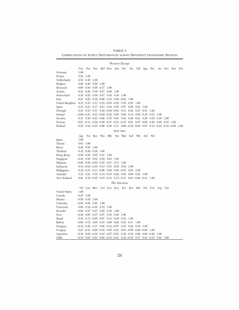
TABLE 5CORRELATIONS OF SUPPLY DISTURBANCES ACROSS DIFFERENT GEOGRAPHIC REGIONS

Western Europe

Ger Fra Net Bel Den Aus Swi Ita UK Spa Por Ire Swe Nor FinGermany 1.00France 0.52 1.00Netherlands 0.54 0.36 1.00Belgium 0.62 0.40 0.56 1.00Denmark 0.68 0.54 0.56 0.37 1.00Austria 0.41 0.28 0.38 0.47 0.49 1.00Switzerland 0.38 0.25 0.58 0.47 0.36 0.39 1.00Italy 0.21 0.28 0.39 −0.00 0.15 0.06 −0.04 1.00United Kingdom 0.12 0.12 0.13 0.12 −0.05 −0.25 0.16 0.28 1.00Spain 0.33 0.21 0.17 0.23 0.22 0.25 0.07 0.20 0.01 1.00Portugal 0.21 0.33 0.11 0.40 −0.04 −0.03 0.13 0.22 0.27 0.51 1.00Ireland −0.00 −0.21 0.11 −0.02 −0.32 0.08 0.08 0.14 0.05 −0.15 0.01 1.00Sweden 0.31 0.30 0.43 0.06 0.35 0.01 0.44 0.46 0.41 0.20 0.39 0.10 1.00Norway −0.27 −0.11 −0.39 −0.26 −0.37 −0.21 −0.18 0.01 0.27 −0.09 0.26 0.08 0.10 1.00Finland 0.22 0.12 −0.25 0.06 0.30 0.11 0.06 −0.32 −0.04 0.07 −0.13 −0.23 −0.10 −0.08 1.00

East Asia

Jap Tai Kor Tha HK Sin Mal Ind Phi Aul NZJapan 1.00Taiwan 0.61 1.00Korea 0.46 0.54 1.00Thailand 0.32 0.59 0.36 1.00Hong Kong 0.29 0.28 0.05 0.31 1.00Singapore −0.10 0.25 0.02 0.29 0.63 1.00Malaysia −0.02 0.06 −0.03 0.35 0.47 0.71 1.00Indonesia 0.14 −0.03 −0.10 0.13 0.53 0.55 0.52 1.00Philippines 0.10 0.37 −0.11 −0.06 0.05 0.05 −0.03 0.03 1.00Australia 0.12 0.21 0.19 0.14 −0.16 −0.22 0.03 0.09 0.23 1.00New Zealand 0.01 0.19 −0.25 0.15 −0.12 0.13 −0.11 0.01 −0.06 −0.41 1.00

The Americas

US Can Mex Col Ven Ecu Per Bra Bol Par Uru Arg ChiUnited States 1.00Canada −0.47 1.00Mexico −0.59 0.35 1.00Colombia −0.02 0.05 0.25 1.00Venezuela 0.09 0.34 −0.42 0.15 1.00Ecuador −0.02 0.37 0.27 0.20 0.36 1.00Peru −0.40 0.05 0.37 0.07 0.10 0.28 1.00Brazil 0.24 0.13 −0.08 0.07 0.13 0.40 0.38 1.00Bolivia −0.65 0.72 0.65 0.18 0.00 0.29 0.54 0.17 1.00Paraguay −0.34 0.45 0.37 0.06 0.12 −0.07 0.16 0.22 0.39 1.00Uruguay 0.27 −0.31 −0.26 −0.35 0.05 −0.21 0.01 −0.06 −0.20 −0.08 1.00Argentina −0.30 0.08 −0.18 0.10 0.27 −0.01 0.36 0.34 0.06 0.06 −0.48 1.00Chile −0.18 0.03 0.23 0.09 −0.33 −0.41 0.19 −0.23 0.17 0.21 −0.33 0.21 1.00

24

United States and Canada and for the United States and Mexico. Itwould appear that the NAFTA countries are affected by very differentsupply conditions. The negative U.S.-Canadian correlation is particularlyinteresting because the raw data indicate that both growth and inflationare positively (and significantly) correlated—as are the demand distur-bances between these two countries (see below).

To test the robustness of this result, we re-ran the model usingOECD data, which covers the longer period from 1960 to 1990. Supplyshocks between the United States and Canada continue to be negativelycorrelated over this longer period, although at −0.12, the correlationcoefficient is smaller in absolute value than in the results for the shorterperiod.2

Correlation of Demand Shocks

Because demand disturbances include the impact of monetary andfiscal policies, they are less likely than supply disturbances to beinformative about regional patterns. As Table 6 shows, all the regionsfeature a number of significant correlations, but no clear geographicpattern emerges in either Europe or the Americas. Asia, however,shows one geographic group of economies with highly correlateddemand shocks, namely, Hong Kong, Indonesia, Malaysia, Singapore,and Thailand, a grouping similar to that identified by the supplydisturbances.

Overall, the correlations of the estimated disturbances provide asignificantly more coherent picture than the one emerging from the rawdata. Three groupings are isolated that could be potential candidates formonetary unification: Germany and her Northern European neighbors;Japan, Korea, and Taiwan; and Hong Kong, Indonesia, Malaysia, andSingapore, plus (possibly) Thailand. No such groupings are apparent inthe Americas. In particular, disturbances to the potential NAFTApartners tend to be negatively correlated, and the correlation of distur-bances between members of MERCOSUR is small and insignificant.

2 In contrast, the positive correlation between demand disturbances for the UnitedStates and Canada becomes larger when the extended data set is used. In a more detailedstudy focusing on NAFTA and using regional data for both the United States and Canada,we came to the same overall conclusion, namely, that the United States, Canada, andMexico do not form a particularly homogeneous regional grouping from the point of viewof macroeconomic disturbances (Bayoumi and Eichengreen, 1994a).

25

TABLE 6CORRELATIONS OF DEMAND DISTURBANCES ACROSS DIFFERENT GEOGRAPHIC REGIONS

Western Europe

Ger Fra Net Bel Den Aus Swi Ita UK Spa Por Ire Swe Nor FinGermany 1.00France 0.30 1.00Netherlands 0.21 0.34 1.00Belgium 0.36 0.53 0.52 1.00Denmark 0.34 0.32 0.20 0.30 1.00Austria 0.32 0.50 0.29 0.56 0.30 1.00Switzerland 0.18 0.42 0.37 0.28 0.22 0.45 1.00Italy 0.22 0.62 0.24 0.49 0.06 0.44 0.32 1.00United Kingdom 0.09 0.20 −0.05 −0.03 −0.00 −0.15 −0.08 0.05 1.00Spain −0.10 0.53 0.11 0.26 0.25 0.30 0.04 0.43 0.23 1.00Portugal 0.24 0.47 0.05 0.45 0.30 0.60 0.36 0.63 0.24 0.32 1.00Ireland 0.06 0.09 0.39 0.00 0.34 −0.12 0.19 −0.08 0.25 0.02 −0.01 1.00Sweden 0.10 0.18 0.29 0.36 0.18 0.02 −0.07 0.25 0.18 −0.01 0.08 0.30 1.00Norway −0.24 0.01 −0.14 −0.24 −0.11 −0.16 −0.11 −0.30 0.13 0.14 −0.19 −0.20 −0.11 1.00Finland 0.10 0.47 0.32 0.60 0.36 0.53 0.30 0.65 0.16 0.40 0.54 0.17 0.33 −0.21 1.00

East Asia

Jap Tai Kor Tha HK Sin Mal Ind Phi Aul NZJapan 1.00Taiwan −0.01 1.00Korea 0.19 0.33 1.00Thailand −0.04 0.54 0.32 1.00Hong Kong 0.23 0.22 0.05 0.43 1.00Singapore −0.09 0.44 0.27 0.70 0.37 1.00Malaysia 0.12 0.41 0.43 0.58 0.54 0.67 1.00Indonesia 0.16 0.17 0.17 0.36 0.62 0.64 0.58 1.00Philippines 0.29 0.09 0.16 0.15 −0.19 −0.05 −0.11 0.04 1.00Australia 0.22 0.20 0.46 0.32 0.32 0.34 0.50 0.05 −0.01 1.00New Zealand 0.00 −0.39 −0.41 0.10 0.43 0.13 0.06 0.09 −0.06 0.21 1.00

The Americas

US Can Mex Col Ven Ecu Per Bra Bol Par Uru Arg ChiUnited States 1.00Canada 0.30 1.00Mexico −0.12 0.37 1.00Colombia 0.07 −0.09 −0.27 1.00Venezuela 0.06 0.47 0.20 0.29 1.00Ecuador 0.19 0.28 −0.21 0.24 0.61 1.00Peru 0.20 0.27 0.50 −0.33 0.05 −0.09 1.00Brazil 0.03 0.59 0.27 0.08 0.70 0.52 0.35 1.00Bolivia 0.09 0.07 0.06 −0.02 −0.20 −0.19 0.18 0.02 1.00Paraguay 0.11 0.50 0.23 0.39 0.51 0.13 −0.04 0.38 −0.18 1.00Uruguay 0.35 0.04 −0.01 0.07 −0.26 −0.45 0.25 0.24 −0.13 0.08 1.00Argentina 0.08 0.07 0.08 −0.08 0.35 0.29 0.35 0.15 0.01 0.33 −0.41 1.00Chile 0.50 0.68 0.06 0.21 0.37 0.37 −0.26 0.11 0.26 0.37 −0.24 0.05 1.00

26

Size of Disturbances

In addition to providing estimates on the correlation of disturbances,our results also convey information about the size and the speed atwhich the respective economies adjust. The larger the disturbances, themore disruptive will be their effects and the greater the premium thatwill be placed, given any cross-country correlation, on instruments(such as monetary policy) that might be used to offset them. Similarly,the slower the response of an economy to disturbances, the larger thecosts of permanently fixing the exchange rate and of foregoing policyautonomy.

Because our econometric procedure restricts the variance of theestimated disturbances to unity, their magnitude can be inferred byconsidering the associated impulse response functions, which trace outthe effect of a unit shock on prices and output. For the supply distur-bances, an obvious measure is the long-run output effect, which measuresthe shift in potential supply (Figure 1). For demand disturbances, wecalculated as a measure of size the sum of the first-year impact on outputand prices, which measures the short-run change in nominal GDP.

Table 7 suggests that Europe and Asia face similarly sized supplyshocks on average, whereas the Americas experience supply shocksalmost twice as large. The Americas also experience relatively largedemand shocks, seven times larger than Europe’s and more than threetimes larger than Asia’s. This is consistent with the greater variability ofgrowth and (especially) inflation in the Americas.3 There is also someevidence that the groups identified on the basis of the underlyingcorrelations experience smaller underlying disturbances, a finding thatlends further support to the viability of these regional groupings asmonetary unions.

Speed of Adjustment

The speed of adjustment is summarized by the response after two yearsas a share of the long-run effect.4 The second and fourth columns ofTable 7 display the results. Asia has the fastest adjustment, with almostall of the change in output and prices occurring within two years. Next

3 Much of this instability may reflect unstable macroeconomic policies. Correspond-ingly, the United States and Canada face demand disturbances the sizes of which aremore akin to those in Europe than to those of the other countries in the region.

4 Although the choice of the second year as the numerator in this calculation issomewhat arbitrary, calculations using other years produced similar results.

27

TABLE 7DISTURBANCES AND ADJUSTMENT ACROSS DIFFERENT GEOGRAPHIC REGIONS

Supply Disturbances Demand Disturbances

Size Adjustment Speed Size Adjustment Speed

Western Europe

Austria 0.018 0.999 0.017 0.415Belgium 0.028 0.668 0.020 0.508Denmark 0.022 1.104 0.017 0.135Finland 0.018 0.875 0.027 0.684France 0.034 0.243 0.014 0.101Germany 0.022 1.193 0.015 0.659Ireland 0.021 1.222 0.038 0.382Italy 0.030 0.427 0.036 0.380Netherlands 0.033 0.692 0.019 0.511Norway 0.031 0.651 0.034 0.704Portugal 0.061 0.426 0.026 0.367Spain 0.057 0.083 0.015 0.123Sweden 0.030 0.261 0.012 0.419Switzerland 0.031 0.997 0.016 0.858United Kingdom 0.018 0.425 0.019 0.016

Average 0.030 0.684 0.022 0.417

East Asia

Australia 0.011 0.925 0.017 0.910Hong Kong 0.023 1.590 0.044 1.190Indonesia 0.013 1.239 0.071 1.335Japan 0.012 1.667 0.017 0.270Korea 0.029 0.886 0.038 0.115Malaysia 0.032 1.038 0.063 1.607New Zealand 0.060 0.648 0.031 0.291Philippines 0.089 0.587 0.081 1.475Singapore 0.032 1.353 0.028 1.072Taiwan 0.021 1.466 0.049 0.673Thailand 0.026 1.381 0.042 1.279

Average 0.032 1.162 0.044 0.929

The Americas

Argentina 0.033 1.141 0.438 1.126Bolivia 0.069 0.585 0.636 1.302Brazil 0.084 0.706 0.068 0.983Canada 0.020 1.052 0.028 0.703Chile 0.064 1.214 0.251 0.548Colombia 0.026 0.823 0.027 0.720Ecuador 0.162 0.402 0.076 0.987Mexico 0.059 0.775 0.072 0.865Paraguay 0.094 0.459 0.064 0.719Peru 0.050 1.169 0.062 0.452United States 0.028 0.269 0.015 0.078Uruguay 0.049 1.014 0.074 1.227Venezuela 0.062 0.810 0.074 0.949

Average 0.062 0.801 0.145 0.820

come the Americas, where, on average, four-fifths of adjustment iscompleted within two years. In Europe, by contrast, only about half ofthe change occurs within two years. The Northern European economies(particularly Belgium, Germany, the Netherlands, and Switzerland) arecharacterized by relatively rapid adjustment, whereas those of SouthernEurope (Italy, Spain, and for these purposes, France) exhibit largedemand disturbances and relatively slow responses. The Philippines andNew Zealand and the United States and Canada appear to be lessflexible than other economies in their respective regions.

Recapitulation

Chapter 2 identified three criteria (related to macroeconomic distur-bances) that are useful for gauging the suitability of countries forparticipation in monetary unions: the size of shocks, their cross-countrycorrelation, and the speed of domestic adjustment. All point towardthree economic groupings that constitute plausible monetary unions: aNorthern European bloc made up of Belgium, Denmark, France,Germany, and the Netherlands; a Northeast Asian bloc comprised ofJapan, Korea, and Taiwan; and a Southeast Asian area made up of HongKong, Indonesia, Malaysia, Singapore, and possibly Thailand. Each ofthese groups is comprised of economies with relatively small disturbances,high correlations across economies, and rapid speeds of adjustment.

29

7 UNITED STATES REGIONAL DATA

This chapter compares the results reported above with those derivedfrom regional data for the United States (for more detail, see Bayoumiand Eichengreen, 1993). The United States is a smoothly functioningcontinental monetary union with regions roughly comparable in size, interms of population and global economic significance, to many of thecountries in our sample. United States data therefore provide a usefulbenchmark for gauging the implications of our results for the viabilityof other potential monetary unions.

Data on real and nominal gross state product were collected for1963 to 1986. These were aggregated into seven regions: New England,Mideast, Great Lakes, Plains, Southeast, Far West, and West.1

The over-identifying restriction regarding the simulated response ofprices was satisfied for every region but the West, where supply shockswere associated with a rise in prices rather than a fall. Like most of thecountries with perverse price responses to supply shocks, this region isdependent on raw-material production (especially crude oil).2

Table 8 reports the correlations of supply and demand disturbancesfor the seven U.S. regions. Six of the seven regions exhibit highlycorrelated supply disturbances, the exception being the West. Twelveof the fifteen cross-correlations for these regions are greater than 0.37,the significance level used in earlier analysis. Three regions, namely,New England, Mideast, and Great Lakes (the “Manufacturing Belt”),have exceptionally highly correlated supply disturbances, with highercorrelations than those for any of the countries analyzed above. Theother correlations are similar in magnitude to those found in the earlieranalysis. By contrast, supply disturbances to the West are negativelycorrelated with most other regions, presumably reflecting the importanceof the oil industry.

1 This is in contrast to the eight regions used by the Bureau of Economic Analysis.The difference is due to our amalgamation of the smallest regions, the Rocky Mountainsand the Southwest, into a combined region, which we call the “West.” The RockyMountains and the Southwest have similar economic structures, and both specializepredominately in primary production. Together they comprise a region comparable insize to other U.S. regions and to foreign countries analyzed in this study.

2 To determine whether the anomalous price response resulted from the aggregationof the two regions, we estimated and simulated the model separately for both and founda perverse price response to supply shocks in each case.

30

The demand disturbances show a similar pattern. Correlations among

TABLE 8CORRELATIONS OF DISTURBANCES ACROSS REGIONS IN THE UNITED STATES

Supply

New Mideast Great Plains Far West

New 1.00Mideast 0.86 1.00Great Lakes 0.77 0.81 1.00Southeast 0.34 0.30 0.46 1.00Plains 0.44 0.67 0.66 0.49 1.00Far West 0.62 0.52 0.65 0.43 0.32 1.00West 0.07 −0.18 −0.11 −0.33 −0.66 0.26 1.00

Demand

New Mideast Great Plains Far West

New 1.00Mideast 0.79 1.00Great Lakes 0.66 0.60 1.00Southeast 0.63 0.51 0.79 1.00Plains 0.51 0.50 0.70 0.69 1.00Far West 0.59 0.33 0.64 0.43 0.30 1.00West 0.26 0.28 0.03 −0.27 −0.23 0.30 1.00

the six regions other than the West are almost always significant,plausibly reflecting the effects of national macroeconomic policies,whereas correlations between the West and the rest of the country aresmaller. The high cross-correlations within the United States contrastwith the results reported in Table 6, consistent with our interpretationthat these disturbances reflect macroeconomic policy.

Table 9 reports the size of the underlying disturbances and the speedof adjustment. The size of disturbances is similar to that found inEurope and, for the supply disturbances, Asia as well. Speeds ofadjustment are comparable to those for the countries we have identifiedas potential participants in monetary unions.

Comparing the results for the U.S. regions with those for thepotential monetary unions we have identified in Europe and East Asia,several features stand out. Most regions of the United States experiencesupply disturbances that are significantly more correlated than aredisturbances in any of the possible monetary unions identified earlier;the correlation coefficients between the New England, Mideast, andGreat Lakes regions are all over 0.75, which is higher than any of theequivalent correlations across countries. By contrast, the United States

31

also contains one region, the West, the underlying supply disturbances

TABLE 9REGIONAL DISTURBANCES AND ADJUSTMENT IN THE UNITED STATES

Supply Disturbances Demand Disturbances

Size Adjustment Speed Size Adjustment Speed

New England 0.032 1.149 0.015 0.433Mideast 0.030 0.876 0.013 0.171Great Lakes 0.040 0.630 0.030 0.050Southeast 0.024 0.083 0.015 0.098Plains 0.024 0.073 0.029 0.286Far West 0.044 0.713 0.011 0.548West 0.020 1.418 0.018 0.319

Average 0.031 0.706 0.019 0.272

of which are negatively correlated with those for the rest of the country;this is not true for any of the potential unions that have been identi-fied. Finally, U.S. regions face supply disturbances that are similar inmagnitude to those faced by individual countries, and the speed ofadjustment for U.S. regions is no faster than that for the countries wehave identified as potential monetary-union members.

Of course, these features are not necessarily exogenous with respectto the existence of the U.S. currency union. The Northeast region of theUnited States has presumably become more integrated over time, andthe West more specialized in raw-material production, as a result of asingle currency. The speed of response to disturbances may also beaffected by the inability of regions to adjust by changing the exchangerate with respect to one another. Overall, however, the results suggestthat several potential monetary unions in other parts of the world arerelatively similar in key respects to the U.S. currency union.

32

8 CONCLUSIONS

We have considered the incidence of supply and demand shocks inWestern Europe, East Asia, and the Americas as a way of identifyingcountries experiencing similar economic disturbances and hence satisfy-ing one of the conditions for forming an optimum currency area. To dothis, we have used a procedure for recovering aggregate supply anddemand disturbances from time-series data.

The results suggest the existence of three regional groupings theeconomies of which face similar underlying disturbances: a NorthernEuropean bloc (Austria, Belgium, Denmark, France, Germany, theNetherlands, and possibly Switzerland); a Northeast Asian bloc (Japan,Korea, and Taiwan); and a Southeast Asian bloc (Hong Kong, Indonesia,Malaysia, Singapore, and possibly Thailand). The correlations amongsupply shocks for these regions are not dissimilar to those found inregional data for the United States. In contrast, the United States facesvery different disturbances than do Canada and Mexico, the other twocountries that might conceivably join it in embracing a common currencyone day. The same is true of the members of MERCOSUR.

We have further considered the size of disturbances and the speedof adjustment of the economies experiencing them. The results reinforcethose derived from the correlation analysis. In Western Europe, whereadjustment tends to be sluggish, implying higher costs of monetaryunification, Germany and her immediate neighbors (with the notableexception of France) display the speediest responses. In Asia, whereresponses are faster, New Zealand and the Philippines, which both haverelatively idiosyncratic disturbances, have slow responses. In theAmericas, in addition to there being little correlation of supply distur-bances across countries, disturbances are large, rendering the region astill less plausible candidate for monetary union. Finally, the size ofdisturbances and speed of adjustment of the countries we have identi-fied (on the basis of these criteria) as plausible candidates for monetaryunion appear to differ little from those evident in regional data for theexisting monetary union of the United States.

The potential monetary unions we have identified share severalfeatures. They tend to form contiguous geographic areas, with only a fewexceptions—such as the inclusion of Hong Kong in the Southeast Asianregion, although even there, all the members border a common body of

33

water. Germany and her neighbors, another potential grouping, have, inaddition, a history of economic integration and policy cooperation. TheNortheast Asian bloc countries (Japan, Korea, and Taiwan) share directforeign-investment and component-supply links. The Southeast Asiangroup members (Hong Kong, Indonesia, Malaysia, Singapore, andThailand) represent the next wave of Asian industrialization and containthe region’s two major financial and commercial centers.

Strikingly, these regions do not correspond closely to either currentor prospective formal trade blocs. The region centered on Germanyexcludes over half of the current members of the EU and includes twolong-standing members of EFTA. Japan, Korea, and Taiwan share noformal preferential trading arrangements. The Southeast Asian groupexcludes the Philippines, which is a member of ASEAN, and includesHong Kong, which is not. The results indicate little similarity betweenthe disturbances experienced by the members of MERCOSUR and areeven more negative about the suitability for monetary union of theprospective members of NAFTA. As the example of the EU shows, thisneed not preclude these regional trading organizations from movingtoward fixed exchange rates and, ultimately, monetary union, althoughit suggests that they will have to surmount obstacles along the way.

What do our results suggest about discussions of the scope formonetary union in different parts of the world? We concentrate onEurope, the region on which much of the controversy has focused, andon the Americas, where regional integration initiatives have recentlycalled attention to exchange-rate policy. Our results support the positionof those (for example, Dornbusch, 1990) who have called for a two-speed monetary union in Europe—with France, Germany, and thesmaller countries of Northern Europe proceeding in the fast lane—andwho suggest that Austria and Switzerland would also be plausiblecandidates for early participation in EMU, once Austria is admitted tothe EU, and should Switzerland choose to apply. A particularly inter-esting feature of our results, given the widespread belief that theviability of EMU hinges on a Franco-German alliance, is the pronounceddifference in France’s position in Tables 2, 3 and 5, 6. Tables 2 and 3,based on the underlying time-series data, suggest that the correlation ofFrench growth and inflation rates with those for other countries is oftenhigher outside than inside Northern Europe, whereas Tables 5 and 6,based on the estimated supply and demand disturbances, suggest thatFrance is logically grouped with the rest of the Northern European bloc.

Our results for the Americas suggest that countries in this regionwould have to undertake very major adjustments in policy and

34

performance in laying the groundwork for monetary union. The negativecorrelation of the supply disturbances affecting the United States, on theone hand, and Canada and Mexico, on the other, is particularly strikingin the context of NAFTA. On the demand side, the correlation is lesspronouncedly negative for Mexico and the United States and insignifi-cantly positive for Canada and the United States, but there, too, majorshifts would have to occur with a transition to a common monetarypolicy. The very different aggregate supply shocks experienced by thethree countries suggest that such a shift might exacerbate dislocationson the real side.1 The results for Argentina and Chile, the aggregatesupply disturbances of which are also negatively correlated with thosefor the United States, suggest that a future expansion of NAFTA toinclude South American participants does not change the picture. InEurope, it is argued that wide exchange-rate fluctuations would fanpolitical opposition to completion of the Single Market on the groundsthat some EU member states were not playing by fair monetary rules;our results suggest that the potential for exchange-rate tensions in thecourse of regional economic integration is even greater in the Americas.

In South America itself, trade liberalization between Argentina andBrazil has heightened tensions over exchange-rate policy. Argentineproducers, living with a recently stabilized peso, complain that therapidly depreciating Brazilian cruzeiro allows its much larger neighborto steal an unfair competitive advantage.2 Clearly, much of this tensionreflects the very different demand disturbances afflicting the twoeconomies (Table 6), but their supply conditions (Table 5) are also onlymodestly correlated, and Brazil suffers from slower adjustment of outputto shocks. This suggests that a common monetary policy directed towardstabilizing the bilateral exchange rate might entail protracted adjustmentproblems. The low supply-side correlations are even more pronouncedfor the smaller MERCOSUR participants Uruguay and Paraguay.

The limitations of the analysis should be recalled. We have focusedon aggregate disturbances, ignoring other factors such as the level ofintraregional trade, which may also be relevant to the benefits ofmonetary union. And we have based inferences about the future on

1 In separate work, we found that supply shocks to Western and Eastern Canada arealso negatively correlated with one another, but, in those regions, extensive interregionalfiscal transfers help to dissipate the resulting tensions (Bayoumi and Eichengreen, 1994a).

2 In late 1993 and early 1994, Argentina responded to the depreciation of the cruzeiroby imposing new duties on imports of Brazilian chemicals, refrigerators, steel, paper,textiles, and agricultural machinery, thereby dealing a setback to MERCOSUR.

35

past data, the properties of which may not be invariant to the monetaryregime. These and other caveats notwithstanding, our analysis has clearimplications. It suggests that a European monetary union might runmore smoothly if limited to a subset of EU members. It indicates thatconditions are more conducive to monetary unification in East Asiathan in the Americas. And it implies that, other things being equal,ASEAN is more likely than either NAFTA or MERCOSUR to be acatalyst for negotiations to stabilize intraregional exchange rates and foreventual moves to establish a regional currency.

36

REFERENCES

Baxter, Marianne, and Alan C. Stockman, “Business Cycles and the ExchangeRate System,” Journal of Monetary Economics, 23 (June 1989), pp. 377-400.

Bayoumi, Tamim, “The Effects of the ERM on Participating Economies,”International Monetary Fund Staff Papers, 39 (June 1992), pp. 330-356.

Bayoumi, Tamim, and Barry Eichengreen, “Shocking Aspects of EuropeanMonetary Integration,” in Francisco Torres and Francesco Giavazzi, eds.,Adjustment and Growth in the European Monetary Union, Cambridge,Cambridge University Press, 1993, pp. 193-229.

———, “Monetary and Exchange Rate Arrangements for NAFTA,” Journal ofDevelopment Economics, 43 (February 1994a), pp. 125-165.

———, “The Political Economy of Fiscal Restrictions: Implications for Europefrom the United States,” European Economic Review, 38 (June 1994b), pp.783-791.

———, “Is There a Conflict Between EC Enlargement and European MonetaryUnification?,” Greek Economic Review (forthcoming 1995).

Blanchard, Olivier, and Lawrence Katz, “Regional Evolutions,” BrookingsPapers on Economic Activity, No. 2 (1992), pp. 1-61.

Blanchard, Olivier, and Danny Quah, “The Dynamic Effects of AggregateDemand and Supply Disturbances,” American Economic Review, 79 (Sep-tember 1989), pp. 655-673.

Bryant, Ralph C., Peter Hooper, and Catherine L. Mann, eds., EvaluatingPolicy Regimes: New Research in Empirical Macroeconomics, WashingtonD.C., Brookings Institution, 1993.

Cohen, Daniel, and Charles Wyplosz, “The European Monetary Union: AnAgnostic Evaluation,” in Ralph C. Bryant, David A. Currie, Jacob A.Frenkel, Paul R. Masson, and Richard Portes, eds., Macroeconomic Policiesin an Interdependent World, Washington D.C., Brookings Institution, 1989,pp. 311-337.

Corden, W. Max, Monetary Integration, Princeton Studies in InternationalFinance No. 93, International Finance Section, Princeton, N.J., PrincetonUniversity, International Finance Section, April 1972.

De Grauwe, Paul, and Wim Vanhaverbeke, “Is Europe an Optimal CurrencyArea? Evidence from Regional Data,” in Paul Masson and Mark Taylor,eds., Policy Issues in the Operation of Currency Unions, Cambridge andNew York, Cambridge University Press, 1993, pp. 111-129.

Eichenbaum, Martin, and Charles Evans, “Some Empirical Evidence on theEffects of Monetary Policy Shocks on Exchange Rates,” National Bureau ofEconomic Research Working Paper No. 4271, Cambridge, Mass., NationalBureau of Economic Research, 1993.

37

Eichengreen, Barry, “Is Europe an Optimum Currency Area?,” in Silvio Bornerand Herbert Grubel, eds., The European Community after 1992: Perspec-tives from the Outside, Basingstoke, Hampshire, Macmillan, 1992, pp. 138-161.

———, “Labor Markets and European Monetary Unification,” in Paul Massonand Mark Taylor, eds., Policy Issues in the Operation of Currency Unions,Cambridge, Cambridge University Press, 1993, pp. 130-162.

———, International Monetary Arrangements for the 21st Century, Washington,D.C., Brookings Institution, 1994.

Goto, Junichi, and Koichi Hamada, “Economic Preconditions for Asian RegionalIntegration,” in Takatoshi Ito and Anne O. Krueger, eds., MacroeconomicLinkage: Savings, Exchange Rates, and Capital Flows, Chicago, Universityof Chicago Press for National Bureau of Economic Research, 1994, pp. 359-385.

Honkapohja, Seppo, and Pentti Pikkarainen, “Country Characteristics and theChoice of the Exchange Rate Regime: Are Mini-Skirts Followed by Maxis?,”CEPR Discussion Paper No. 774, London, Centre for Economic PolicyResearch, December 1992.

Ishiyama, Yoshihide, “The Theory of Optimal Currency Areas: A Survey,”International Monetary Fund Staff Papers, 22 (July 1975), pp. 344-383.

Kendall, Maurice G., and Alan Stuart, The Advanced Theory of Statistics, Vol.2, New York, Hafner, 1967.

Kenen, Peter B., “The Theory of Optimum Currency Areas: An Eclectic View,”in Robert A. Mundell and Alexander K. Swoboda, eds., Monetary Problemsof the International Economy, Chicago and London, University of ChicagoPress, 1969, pp. 41-60.

McKinnon, Ronald I., “Optimum Currency Areas,” American Economic Review,53 (September 1963), pp. 717-724.

Mundell, Robert A., “A Theory of Optimum Currency Areas,” AmericanEconomic Review, 51 (September 1961), pp. 657-664.

Organisation for Economic Co-operation and Development (OECD), Flexibilityin the Labour Market, Paris, Organisation for Economic Co-operation andDevelopment, 1987.

Poloz, Stephen S., “Real Exchange Rate Adjustment Between Regions in aCommon Currency Area,” Ottawa, Bank of Canada, 1990, processed.

Romer, Christina, and David Romer, “Does Monetary Policy Matter? A NewTest in the Spirit of Friedman and Schwartz,” NBER MacroeconomicsAnnual (1989), pp. 121-170.

Stern, Gabriel, and Tamim Bayoumi, “Temporary Cycles on Volatile Trends?Economic Fluctuations in 21 OECD Countries,” London, Bank of EnglandWorking Paper No. 13, April 1993.

Tavlas, George S., “The ‘New’ Theory of Optimal Currency Areas,” Washington,D.C., International Monetary Fund, 1992, processed.

38

Torre, Augusto de la, and Margaret R. Kelly, Regional Trade Arrangements,Occasional Paper No. 93, Washington, D.C., International Monetary Fund,March 1992.

Weber, Axel A., “EMU and Asymmetries and Adjustment Problems in theEMS—Some Empirical Evidence,” European Economy, Special Edition No.1 (1991), pp. 187-207.

39

PUBLICATIONS OF THEINTERNATIONAL FINANCE SECTION

Notice to Contributors

The International Finance Section publishes papers in four series: ESSAYS IN INTER-NATIONAL FINANCE, PRINCETON STUDIES IN INTERNATIONAL FINANCE, and SPECIALPAPERS IN INTERNATIONAL ECONOMICS contain new work not published elsewhere.REPRINTS IN INTERNATIONAL FINANCE reproduce journal articles previously pub-lished by Princeton faculty members associated with the Section. The Sectionwelcomes the submission of manuscripts for publication under the followingguidelines:

ESSAYS are meant to disseminate new views about international financial mattersand should be accessible to well-informed nonspecialists as well as to professionaleconomists. Technical terms, tables, and charts should be used sparingly; mathemat-ics should be avoided.

STUDIES are devoted to new research on international finance, with preferencegiven to empirical work. They should be comparable in originality and technicalproficiency to papers published in leading economic journals. They should be ofmedium length, longer than a journal article but shorter than a book.

SPECIAL PAPERS are surveys of research on particular topics and should besuitable for use in undergraduate courses. They may be concerned with internationaltrade as well as international finance. They should also be of medium length.

Manuscripts should be submitted in triplicate, typed single sided and doublespaced throughout on 8½ by 11 white bond paper. Publication can be expedited ifmanuscripts are computer keyboarded in WordPerfect 5.1 or a compatible program.Additional instructions and a style guide are available from the Section.

How to Obtain Publications

The Section’s publications are distributed free of charge to college, university, andpublic libraries and to nongovernmental, nonprofit research institutions. Eligibleinstitutions may ask to be placed on the Section’s permanent mailing list.

Individuals and institutions not qualifying for free distribution may receive allpublications for the calendar year for a subscription fee of $35.00. Late subscriberswill receive all back issues for the year during which they subscribe. Subscribersshould notify the Section promptly of any change in address, giving the old addressas well as the new.

Publications may be ordered individually, with payment made in advance. ESSAYSand REPRINTS cost $8.00 each; STUDIES and SPECIAL PAPERS cost $11.00. Anadditional $1.25 should be sent for postage and handling within the United States,Canada, and Mexico; $1.50 should be added for surface delivery outside the region.

All payments must be made in U.S. dollars. Subscription fees and charges forsingle issues will be waived for organizations and individuals in countries whereforeign-exchange regulations prohibit dollar payments.

Please address all correspondence, submissions, and orders to:

International Finance SectionDepartment of Economics, Fisher HallPrinceton UniversityPrinceton, New Jersey 08544-1021

41

List of Recent Publications

A complete list of publications may be obtained from the International FinanceSection.

ESSAYS IN INTERNATIONAL FINANCE

158. Charles E. Dumas, The Effects of Government Deficits: A ComparativeAnalysis of Crowding Out. (October 1985)

159. Jeffrey A. Frankel, Six Possible Meanings of “Overvaluation”: The 1981-85Dollar. (December 1985)

160. Stanley W. Black, Learning from Adversity: Policy Responses to Two OilShocks. (December 1985)

161. Alexis Rieffel, The Role of the Paris Club in Managing Debt Problems.(December 1985)

162. Stephen E. Haynes, Michael M. Hutchison, and Raymond F. Mikesell,Japanese Financial Policies and the U.S. Trade Deficit. (April 1986)

163. Arminio Fraga, German Reparations and Brazilian Debt: A ComparativeStudy. (July 1986)

164. Jack M. Guttentag and Richard J. Herring, Disaster Myopia in InternationalBanking. (September 1986)

165. Rudiger Dornbusch, Inflation, Exchange Rates, and Stabilization. (October1986)

166. John Spraos, IMF Conditionality: Ineffectual, Inefficient, Mistargeted. (De-cember 1986)

167. Rainer Stefano Masera, An Increasing Role for the ECU: A Character inSearch of a Script. (June 1987)

168. Paul Mosley, Conditionality as Bargaining Process: Structural-AdjustmentLending, 1980-86. (October 1987)

169. Paul A. Volcker, Ralph C. Bryant, Leonhard Gleske, Gottfried Haberler,Alexandre Lamfalussy, Shijuro Ogata, Jesús Silva-Herzog, Ross M. Starr,James Tobin, and Robert Triffin, International Monetary Cooperation: Essaysin Honor of Henry C. Wallich. (December 1987)

170. Shafiqul Islam, The Dollar and the Policy-Performance-Confidence Mix. (July1988)

171. James M. Boughton, The Monetary Approach to Exchange Rates: What NowRemains? (October 1988)

172. Jack M. Guttentag and Richard M. Herring, Accounting for Losses OnSovereign Debt: Implications for New Lending. (May 1989)

173. Benjamin J. Cohen, Developing-Country Debt: A Middle Way. (May 1989)174. Jeffrey D. Sachs, New Approaches to the Latin American Debt Crisis. (July 1989)175. C. David Finch, The IMF: The Record and the Prospect. (September 1989)176. Graham Bird, Loan-Loss Provisions and Third-World Debt. (November 1989)177. Ronald Findlay, The “Triangular Trade” and the Atlantic Economy of the

Eighteenth Century: A Simple General-Equilibrium Model. (March 1990)178. Alberto Giovannini, The Transition to European Monetary Union. (November

1990)

42

179. Michael L. Mussa, Exchange Rates in Theory and in Reality. (December 1990)180. Warren L. Coats, Jr., Reinhard W. Furstenberg, and Peter Isard, The SDR

System and the Issue of Resource Transfers. (December 1990)181. George S. Tavlas, On the International Use of Currencies: The Case of the

Deutsche Mark. (March 1991)182. Tommaso Padoa-Schioppa, ed., with Michael Emerson, Kumiharu Shigehara,

and Richard Portes, Europe After 1992: Three Essays. (May 1991)183. Michael Bruno, High Inflation and the Nominal Anchors of an Open Economy.

(June 1991)184. Jacques J. Polak, The Changing Nature of IMF Conditionality. (September 1991)185. Ethan B. Kapstein, Supervising International Banks: Origins and Implications

of the Basle Accord. (December 1991)186. Alessandro Giustiniani, Francesco Papadia, and Daniela Porciani, Growth and

Catch-Up in Central and Eastern Europe: Macroeconomic Effects on WesternCountries. (April 1992)

187. Michele Fratianni, Jürgen von Hagen, and Christopher Waller, The MaastrichtWay to EMU. (June 1992)

188. Pierre-Richard Agénor, Parallel Currency Markets in Developing Countries:Theory, Evidence, and Policy Implications. (November 1992)

189. Beatriz Armendariz de Aghion and John Williamson, The G-7’s Joint-and-SeveralBlunder. (April 1993)

190. Paul Krugman, What Do We Need to Know About the International MonetarySystem?. (July 1993)

191. Peter M. Garber and Michael G. Spencer, The Dissolution of the Austro-Hungarian Empire: Lessons for Currency Reform. (February 1994)

192. Raymond F. Mikesell, The Bretton Woods Debates: A Memoir. (March 1994)193. Graham Bird, Economic Assistance to Low-Income Countries: Should the Link

be Resurrected?. (July 1994)

PRINCETON STUDIES IN INTERNATIONAL FINANCE

57. Stephen S. Golub, The Current-Account Balance and the Dollar: 1977-78 and1983-84. (October 1986)

58. John T. Cuddington, Capital Flight: Estimates, Issues, and Explanations. (De-cember 1986)

59. Vincent P. Crawford, International Lending, Long-Term Credit Relationships,and Dynamic Contract Theory. (March 1987)

60. Thorvaldur Gylfason, Credit Policy and Economic Activity in DevelopingCountries with IMF Stabilization Programs. (August 1987)

61. Stephen A. Schuker, American “Reparations” to Germany, 1919-33: Implicationsfor the Third-World Debt Crisis. (July 1988)

62. Steven B. Kamin, Devaluation, External Balance, and Macroeconomic Perfor-mance: A Look at the Numbers. (August 1988)

63. Jacob A. Frenkel and Assaf Razin, Spending, Taxes, and Deficits: International-Intertemporal Approach. (December 1988)

64. Jeffrey A. Frankel, Obstacles to International Macroeconomic Policy Coordina-tion. (December 1988)

43

65. Peter Hooper and Catherine L. Mann, The Emergence and Persistence of theU.S. External Imbalance, 1980-87. (October 1989)

66. Helmut Reisen, Public Debt, External Competitiveness, and Fiscal Disciplinein Developing Countries. (November 1989)

67. Victor Argy, Warwick McKibbin, and Eric Siegloff, Exchange-Rate Regimes fora Small Economy in a Multi-Country World. (December 1989)

68. Mark Gersovitz and Christina H. Paxson, The Economies of Africa and the Pricesof Their Exports. (October 1990)

69. Felipe Larraín and Andrés Velasco, Can Swaps Solve the Debt Crisis? Lessonsfrom the Chilean Experience. (November 1990)

70. Kaushik Basu, The International Debt Problem, Credit Rationing and LoanPushing: Theory and Experience. (October 1991)

71. Daniel Gros and Alfred Steinherr, Economic Reform in the Soviet Union: Pasde Deux between Disintegration and Macroeconomic Destabilization. (November1991)

72. George M. von Furstenberg and Joseph P. Daniels, Economic Summit Decla-rations, 1975-1989: Examining the Written Record of International Coopera-tion. (February 1992)

73. Ishac Diwan and Dani Rodrik, External Debt, Adjustment, and Burden Sharing:A Unified Framework. (November 1992)

74. Barry Eichengreen, Should the Maastricht Treaty Be Saved?. (December 1992)75. Adam Klug, The German Buybacks, 1932-1939: A Cure for Overhang?.

(November 1993)76. Tamim Bayoumi and Barry Eichengreen, One Money or Many? Analyzing the

Prospects for Monetary Unification in Various Parts of the World. (September1994)

SPECIAL PAPERS IN INTERNATIONAL ECONOMICS

15. Gene M. Grossman and J. David Richardson, Strategic Trade Policy: A Surveyof Issues and Early Analysis. (April 1985)

16. Elhanan Helpman, Monopolistic Competition in Trade Theory. (June 1990)17. Richard Pomfret, International Trade Policy with Imperfect Competition. (August

1992)18. Hali J. Edison, The Effectiveness of Central-Bank Intervention: A Survey of the

Literature After 1982. (July 1993)

REPRINTS IN INTERNATIONAL FINANCE

25. Jorge Braga de Macedo, Trade and Financial Interdependence under FlexibleExchange Rates: The Pacific Area; reprinted from Pacific Growth and FinancialInterdependence, 1986. (June 1986)

26. Peter B. Kenen, The Use of IMF Credit; reprinted from Pulling Together: TheInternational Monetary Fund in a Multipolar World, 1989. (December 1989)

27. Peter B. Kenen, Transitional Arrangements for Trade and Payments Among theCMEA Countries; reprinted from International Monetary Fund Staff Papers 38(2), 1991. (July 1991)

44

The work of the International Finance Section is supportedin part by the income of the Walker Foundation, establishedin memory of James Theodore Walker, Class of 1927. Theoffices of the Section, in Fisher Hall, were provided by agenerous grant from Merrill Lynch & Company.

ISBN 0-88165-248-2Recycled Paper