OnAutoencodersandScoreMatchingforEnergy...
35
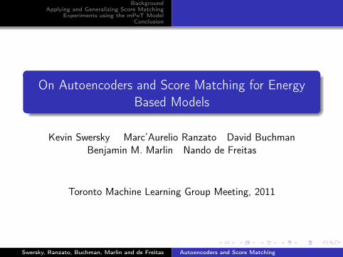
Background Applying and Generalizing Score Matching Experiments using the mPoT Model Conclusion On Autoencoders and Score Matching for Energy Based Models Kevin Swersky Marc’Aurelio Ranzato David Buchman Benjamin M. Marlin Nando de Freitas Toronto Machine Learning Group Meeting, 2011 Swersky, Ranzato, Buchman, Marlin and de Freitas Autoencoders and Score Matching
Transcript of OnAutoencodersandScoreMatchingforEnergy...
BackgroundApplying and Generalizing Score Matching
Experiments using the mPoT ModelConclusion
On Autoencoders and Score Matching for EnergyBased Models
Kevin Swersky Marc’Aurelio Ranzato David BuchmanBenjamin M. Marlin Nando de Freitas
Toronto Machine Learning Group Meeting, 2011
Swersky, Ranzato, Buchman, Marlin and de Freitas Autoencoders and Score Matching

BackgroundApplying and Generalizing Score Matching
Experiments using the mPoT ModelConclusion
MotivationModelsLearning
Goal: Unsupervised Feature Learning
Automatically learn features from dataUseful for modeling images, speech, text, etc. withoutrequiring lots of prior knowledgeMany models and algorithms, we will focus on two commonlyused ones
Swersky, Ranzato, Buchman, Marlin and de Freitas Autoencoders and Score Matching

BackgroundApplying and Generalizing Score Matching
Experiments using the mPoT ModelConclusion
MotivationModelsLearning
Motivation
Autoencoders and energy based models represent thestate-of-the-art for feature learning in several domainsWe provide some unifying theory for these model familiesThis will allow us to derive new autoencoder architecturesfrom energy based modelsIt will also give us an interesting way to regularize theseautoencoders
Swersky, Ranzato, Buchman, Marlin and de Freitas Autoencoders and Score Matching

BackgroundApplying and Generalizing Score Matching
Experiments using the mPoT ModelConclusion
MotivationModelsLearning
Latent Energy Based Models
A probability distribution over datavectors v , with latent variables hand parameters θ
Defined using an energy functionEθ (v ,h) as:
Pθ (v) =exp(−Eθ (v ,h))
Z (θ)
Normalized by the partitionfunctionZ (θ) =
∫v∫h exp(−Eθ (v ,h))dhdv
Z (θ) is usually not analyticalFeatures given by h
...
...h1 h2 hnh
v1 v2 vnv
Restricted BoltzmannMachine
...h1 h2 hnh
...v1 v2 vnv ...v1 v2 vnv
Factored EBM (e.g. mPoT)
Swersky, Ranzato, Buchman, Marlin and de Freitas Autoencoders and Score Matching
BackgroundApplying and Generalizing Score Matching
Experiments using the mPoT ModelConclusion
MotivationModelsLearning
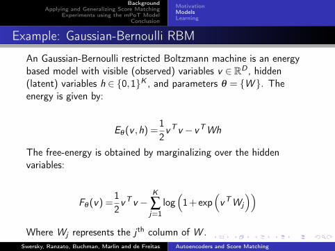
Example: Gaussian-Bernoulli RBM
An Gaussian-Bernoulli restricted Boltzmann machine is an energybased model with visible (observed) variables v ∈ RD , hidden(latent) variables h ∈ 0,1K , and parameters θ = W . Theenergy is given by:
Eθ (v ,h) =12vT v − vTWh
The free-energy is obtained by marginalizing over the hiddenvariables:
Fθ (v) =12vT v −
K
∑j=1
log(1+ exp
(vTWj
))Where Wj represents the j th column of W .
Swersky, Ranzato, Buchman, Marlin and de Freitas Autoencoders and Score Matching

BackgroundApplying and Generalizing Score Matching
Experiments using the mPoT ModelConclusion
MotivationModelsLearning
Autoencoders
A feed-forward neural network designed toreconstruct its input
Encoding function: gθ (v)
Reconstruction function: fθ (gθ (v))
Minimizes reconstruction error:
θ =argminθ
||fθ (gθ (v))− v ||2
Features given by gθ (v)
v
fθ(gθ(v))
gθ(v)
Swersky, Ranzato, Buchman, Marlin and de Freitas Autoencoders and Score Matching

BackgroundApplying and Generalizing Score Matching
Experiments using the mPoT ModelConclusion
MotivationModelsLearning
Example: One-Layer Autoencoder
A commonly used autoencoder architecture maps inputs v ∈ RD tooutputs v ∈ RD through a deterministic hidden layer h ∈ [0,1]K
using parameters θ = W by the following system:
v =fθ (gθ (v)) = Wh
h =gθ (v) = σ(W T v)
Where σ(x) = 11+exp(−x) .
We train this by minimizing the reconstruction error:
`(θ) =D
∑i=1
12
(vi − vi )2
Swersky, Ranzato, Buchman, Marlin and de Freitas Autoencoders and Score Matching

BackgroundApplying and Generalizing Score Matching
Experiments using the mPoT ModelConclusion
MotivationModelsLearning
Comparison
Energy based models Autoencoders
UndirectedProbabilisticSlow inferenceIntractable objectivefunction
DirectedDeterministicFast inferenceTractable objectivefunction
Unifying these model families lets us leverage the advantagesof each
Swersky, Ranzato, Buchman, Marlin and de Freitas Autoencoders and Score Matching

BackgroundApplying and Generalizing Score Matching
Experiments using the mPoT ModelConclusion
MotivationModelsLearning
Maximum Likelihood for EBMs
Minimize KL divergence between empirical data distributionP(v) and model distribution Pθ (v):
θ =argminθ
Ep(v)
[log(P(v))− log(Pθ (v))
]
v
log(P(v))
P(v)Pθ(v)
~
Requires that we know Z (θ)Idea: Approximate Z (θ) with samples from Pθ (v)
Uses MCMCContrastive divergence (CD), persistent contrastive divergence(PCD), fast PCD (FPCD)
Swersky, Ranzato, Buchman, Marlin and de Freitas Autoencoders and Score Matching

BackgroundApplying and Generalizing Score Matching
Experiments using the mPoT ModelConclusion
MotivationModelsLearning
Score Matching (Hyvarinen, 2006)
Intuition: If two functions have the same derivativeseverywhere, then they are the same functions up to a constantWe match ∂
∂vilog(P(v)
)and ∂
∂vilog (Pθ (v))
The constraint∫v P(v)dv = 1 means that the distributions
must be equal if their derivatives are perfectly matched
Swersky, Ranzato, Buchman, Marlin and de Freitas Autoencoders and Score Matching
BackgroundApplying and Generalizing Score Matching
Experiments using the mPoT ModelConclusion
MotivationModelsLearning
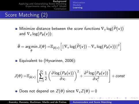
Score Matching (2)
Minimize distance between the score functions ∇v log(P(v))and ∇v log(Pθ (v)):
θ = argminθ
J(θ) =Ep(v)
[||∇v log(P(v))−∇v log(Pθ (v))||2
]Equivalent to (Hyvarinen, 2006):
J(θ) =Ep(v)
[D
∑i=1
12
(∂ log (Pθ (v))
∂vi
)2
+∂ 2 log (Pθ (v))
∂v2i
]+ const
Does not depend on Z (θ) since ∇vZ (θ) = 0
Swersky, Ranzato, Buchman, Marlin and de Freitas Autoencoders and Score Matching

BackgroundApplying and Generalizing Score Matching
Experiments using the mPoT ModelConclusion
MotivationModelsLearning
Score Matching (3)
Score matching is not as statistically efficient as maximumlikelihood
It is in fact an approximation to pseudolikelihood (Hyvarinen,2006)
Statistical efficiency is only beneficial if you can actually findgood parametersWe trade efficiency for the ability to find better parameterswith more powerful optimization
Swersky, Ranzato, Buchman, Marlin and de Freitas Autoencoders and Score Matching

BackgroundApplying and Generalizing Score Matching
Experiments using the mPoT ModelConclusion
MotivationModelsLearning
Denoising Score Matching (Vincent, 2011)
Rough idea:1 Apply a kernel qβ (v |v ′) to P(v) get a smoothed distribution
qβ (v) =∫
qβ (v |v ′)P(v ′)dv ′2 Apply score matching to qβ (v)
Faster than ordinary score matching (no 2nd derivatives)Includes denoising autoencoders (for continuous data) as aspecial case
Data
Likelihood
Pθ (v)Data
Likelihood
qβ (v)
Swersky, Ranzato, Buchman, Marlin and de Freitas Autoencoders and Score Matching
BackgroundApplying and Generalizing Score Matching
Experiments using the mPoT ModelConclusion
ExamplesGeneralization and InterpretationConnections with Autoencoders
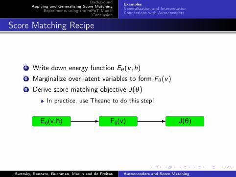
Score Matching Recipe
1 Write down energy function Eθ (v ,h)
2 Marginalize over latent variables to form Fθ (v)
3 Derive score matching objective J(θ)
In practice, use Theano to do this step!
Eθ(v,h) Fθ(v) J(θ)
Swersky, Ranzato, Buchman, Marlin and de Freitas Autoencoders and Score Matching

BackgroundApplying and Generalizing Score Matching
Experiments using the mPoT ModelConclusion
ExamplesGeneralization and InterpretationConnections with Autoencoders
Example: RBM with All Gaussian Units
If both v and h are Gaussian-distributed, we have the followingenergy and free-energy:
Eθ (v ,h) =12vT v +
12hTh− vTWh
Fθ (v) =12vT(I−WW T
)v
J(θ) =D
∑i=1
12
(vi −
K
∑j=1
Wij
(W T
j v))2
+K
∑j=1
W 2ij
This is a linear autoencoder with weight-decay regularization
Swersky, Ranzato, Buchman, Marlin and de Freitas Autoencoders and Score Matching

BackgroundApplying and Generalizing Score Matching
Experiments using the mPoT ModelConclusion
ExamplesGeneralization and InterpretationConnections with Autoencoders
Example: RBM with All Gaussian Units (2)
With denoising score matching:
J(θ) =D
∑i=1
12
(vi −
K
∑j=1
Wij
(W T
j x))2
x ∼N(v ,σ2I)
Adding noise to the input is roughly equivalent toweight-decay (Bishop, 1994)
Swersky, Ranzato, Buchman, Marlin and de Freitas Autoencoders and Score Matching

BackgroundApplying and Generalizing Score Matching
Experiments using the mPoT ModelConclusion
ExamplesGeneralization and InterpretationConnections with Autoencoders
Example: Gaussian-Bernoulli RBMs
We apply score matching to the GBRBM model:
J(θ) =const +D
∑i=1
[12
(vi − vi )2 +
K
∑j=1
W 2ij hj
(1− hj
)]
This is also a regularized autoencoderThe regularizer is a sum of weighted variances of the Bernoullirandom variables h conditioned on v
Swersky, Ranzato, Buchman, Marlin and de Freitas Autoencoders and Score Matching

BackgroundApplying and Generalizing Score Matching
Experiments using the mPoT ModelConclusion
ExamplesGeneralization and InterpretationConnections with Autoencoders
Example: mPoT (Warning: lots of equations!)
The GBRBM is bad at modelling heavy-tailed distributions,and capturing covariance structure in vWe can use more sophisticated energy-based models toovercome these limitations
The mPoT is an energy based model with Gaussian-distributedvisible units, Gamma-distributed hidden units hc ∈ R+K , andBernoulli-distributed hidden units hm ∈ 0,1M with parametersθ = C ,W .
Eθ (v ,hm,hc) =K
∑k=1
[hck(1+
12
(CTk v)2) + (1− γ) log(hc
k)
]+
12vT v −vTWhm
Fθ (v) =K
∑k=1
γ log(1+12
(φck )2)−
M
∑j=1
log(1+ eφmj ) +
12vT v
φck =CT
k v
φmj =W T
j v
Swersky, Ranzato, Buchman, Marlin and de Freitas Autoencoders and Score Matching

BackgroundApplying and Generalizing Score Matching
Experiments using the mPoT ModelConclusion
ExamplesGeneralization and InterpretationConnections with Autoencoders
Example: mPoT (2) (Warning: lots of equations!)
J(θ) =D
∑i=1
12
ψi (pθ (v))2 +K
∑k=1
(ρ(hc
k)D2ik + hc
kKik
)+
M
∑j=1
(hmj (1− hm
j )W 2ij
)−1
ψi (pθ (v)) =K
∑k=1
hckDik +
M
∑j=1
hmj Wij −vi
Kik =K
∑k=1−C 2
ik
Dik =K
∑k=1
(−(CT
k v)Cik)
hck =
γ
1+ 12 (φ c
k )2
hmj =sigm(φ
mj )
ρ(x) =x2
Swersky, Ranzato, Buchman, Marlin and de Freitas Autoencoders and Score Matching

BackgroundApplying and Generalizing Score Matching
Experiments using the mPoT ModelConclusion
ExamplesGeneralization and InterpretationConnections with Autoencoders
Score Matching for General Latent EBMs
Score matching can produce complicated and difficult tointerpret objective functionsOur solution is to apply score matching to latent EBMswithout directly specifying Eθ (v ,h)
Swersky, Ranzato, Buchman, Marlin and de Freitas Autoencoders and Score Matching

BackgroundApplying and Generalizing Score Matching
Experiments using the mPoT ModelConclusion
ExamplesGeneralization and InterpretationConnections with Autoencoders
Score Matching for General Latent EBMs (2)
TheoremThe score matching objective for a latent EBM can be expressedsuccinctly in terms of expectations of the energy with respect tothe conditional distribution Pθ (h|v).
J(θ) = Ep(v)
[nv
∑i=1
12
(Epθ (h|v)
[∂Eθ (v ,h)
∂vi
])2
+ varpθ (h|v)
[∂Eθ (v ,h)
∂vi
]−Epθ (h|v)
[∂ 2Eθ (v ,h)
∂v2i
]].
The score matching objective for a latent EBM always consistsof 3 terms:
1 Squared error2 Variance of error3 Curvature
Variance and curvature can be seen as regularizers
Swersky, Ranzato, Buchman, Marlin and de Freitas Autoencoders and Score Matching

BackgroundApplying and Generalizing Score Matching
Experiments using the mPoT ModelConclusion
ExamplesGeneralization and InterpretationConnections with Autoencoders
Visualization
Data
Likelihood
Model probability before learning
Vari-anceandCur-va-tureshapethedis-tri-bu-tion
Squareder-rorcen-tersmassondata
Swersky, Ranzato, Buchman, Marlin and de Freitas Autoencoders and Score Matching

BackgroundApplying and Generalizing Score Matching
Experiments using the mPoT ModelConclusion
ExamplesGeneralization and InterpretationConnections with Autoencoders
Visualization
Data
Likelihood
Model probability before learning
Vari-anceandCur-va-tureshapethedis-tri-bu-tion
Data
Likelihood
Squared error centers mass on data
Swersky, Ranzato, Buchman, Marlin and de Freitas Autoencoders and Score Matching

BackgroundApplying and Generalizing Score Matching
Experiments using the mPoT ModelConclusion
ExamplesGeneralization and InterpretationConnections with Autoencoders
Visualization
Data
Likelihood
Model probability before learning
Data
Likelihood
Variance and Curvature shape thedistribution
Data
Likelihood
Squared error centers mass on data
Swersky, Ranzato, Buchman, Marlin and de Freitas Autoencoders and Score Matching
BackgroundApplying and Generalizing Score Matching
Experiments using the mPoT ModelConclusion
ExamplesGeneralization and InterpretationConnections with Autoencoders
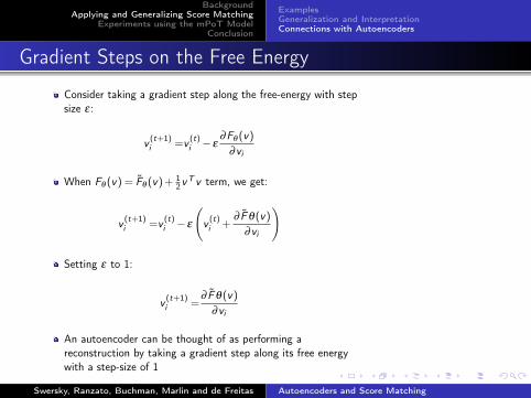
Gradient Steps on the Free Energy
Consider taking a gradient step along the free-energy with stepsize ε :
v (t+1)i =v (t)
i − ε∂Fθ (v)
∂vi
When Fθ (v) = Fθ (v) + 12vT v term, we get:
v (t+1)i =v (t)
i − ε
(v (t)i +
∂ Fθ(v)
∂vi
)
Setting ε to 1:
v (t+1)i =
∂ Fθ(v)
∂vi
An autoencoder can be thought of as performing areconstruction by taking a gradient step along its free energywith a step-size of 1
Swersky, Ranzato, Buchman, Marlin and de Freitas Autoencoders and Score Matching
BackgroundApplying and Generalizing Score Matching
Experiments using the mPoT ModelConclusion
ExamplesGeneralization and InterpretationConnections with Autoencoders
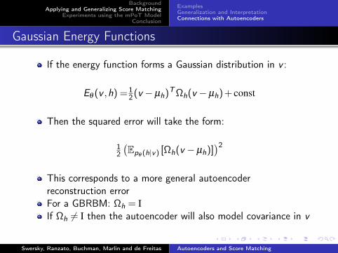
Gaussian Energy Functions
If the energy function forms a Gaussian distribution in v :
Eθ (v ,h) =12(v −µh)T Ωh(v −µh) + const
Then the squared error will take the form:
12
(Epθ (h|v) [Ωh(v −µh)]
)2This corresponds to a more general autoencoderreconstruction errorFor a GBRBM: Ωh = IIf Ωh 6= I then the autoencoder will also model covariance in v
Swersky, Ranzato, Buchman, Marlin and de Freitas Autoencoders and Score Matching

BackgroundApplying and Generalizing Score Matching
Experiments using the mPoT ModelConclusion
Objectives
Can we learn good features with richer autoencoder models?How do score matching estimators compare to maximumlikelihood estimators?What are the effects of regularization in a scorematching-based autoencoder?
Swersky, Ranzato, Buchman, Marlin and de Freitas Autoencoders and Score Matching

BackgroundApplying and Generalizing Score Matching
Experiments using the mPoT ModelConclusion
Learned Features
Covariance filters
Swersky, Ranzato, Buchman, Marlin and de Freitas Autoencoders and Score Matching
BackgroundApplying and Generalizing Score Matching
Experiments using the mPoT ModelConclusion
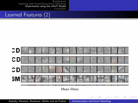
Learned Features (2)
Mean filters
Swersky, Ranzato, Buchman, Marlin and de Freitas Autoencoders and Score Matching

BackgroundApplying and Generalizing Score Matching
Experiments using the mPoT ModelConclusion
Denoising
Reconstruct an image from a blurry versionFinds a nearby image that has a high likelihood
0 20 40 60 80 1000.35
0.4
0.45
0.5
0.55
0.6
0.65
0.7
Epoch
MS
E
FPCD
PCD
CD
SM
SMD
Swersky, Ranzato, Buchman, Marlin and de Freitas Autoencoders and Score Matching

BackgroundApplying and Generalizing Score Matching
Experiments using the mPoT ModelConclusion
Classification on CIFAR-10
CD PCD FPCD SM SMD AE64.6% 64.7% 65.5% 65.0% 64.7% 57.6%
Most methods are comparablemPoT autoencoder without regularization does significantlyworse
Swersky, Ranzato, Buchman, Marlin and de Freitas Autoencoders and Score Matching

BackgroundApplying and Generalizing Score Matching
Experiments using the mPoT ModelConclusion
Effect of Regularizers on mPoT Autoencoder
Score matching mPoT autoencoder(×104)
0 20 40 60 80 100−300
−200
−100
0
100
200
Epoch
Valu
e
Total
Recon
Var
Curve
Autoencoder with no regularization
Total (blue curve) is the sum of the other curvesOther curves represent the 3 score matching terms
Swersky, Ranzato, Buchman, Marlin and de Freitas Autoencoders and Score Matching

BackgroundApplying and Generalizing Score Matching
Experiments using the mPoT ModelConclusion
Quick Mention: Memisevic, 2011
Roland Memisevic, a recent U of T grad published a paper inthis year’s ICCVHe derived the same models through the idea of relating twodifferent inputs using an autoencoder
Swersky, Ranzato, Buchman, Marlin and de Freitas Autoencoders and Score Matching
BackgroundApplying and Generalizing Score Matching
Experiments using the mPoT ModelConclusion
Conclusion
Score matching provides a unifying theory for autoencodersand latent energy based modelsIt reveals novel regularizers for some modelsWe can derive novel autoencoders that model richer structureWe provide an interpretation of the score matching objectivefor all latent EBMsProperly shaping the implied energy of an autoencoder is onekey to learning good features
This is done implicitly when noise is added to the inputPerhaps also done implicity with sparsity penalties, etc.
Swersky, Ranzato, Buchman, Marlin and de Freitas Autoencoders and Score Matching
BackgroundApplying and Generalizing Score Matching
Experiments using the mPoT ModelConclusion
Future Work
We can model other kinds of data with higher-order featuresby simply changing the loss functionExtend higher-order models to deeper layersApply Hessian-free optimization to EBMs and relatedautoencoders
Swersky, Ranzato, Buchman, Marlin and de Freitas Autoencoders and Score Matching