On Wireless Local Area Networks - Hamilton Institute · On Wireless Local Area Networks A...

On Wireless Local Area Networks

A dissertation submitted for the degree of

Doctor of Philosophy

by

Kaidi Huang

Research Supervisor: Dr. Ken Duffy

Head of Department: Prof. Douglas Leith

Hamilton Institute

National University of Ireland Maynooth

Maynooth, Co. Kildare

Republic of Ireland

December 2010

Contents

1 Introduction 1

1.1 Wireless Local Area Networks . . . . . . . . . . . . . . . . . . . . . . . . . . . . . . . . 1

1.1.1 Types of WLANs . . . . . . . . . . . . . . . . . . . . . . . . . . . . . . . . . . . 1

1.1.2 Advantages of WLANs . . . . . . . . . . . . . . . . . . . . . . . . . . . . . . . . 3

1.2 IEEE 802.11 . . . . . . . . . . . . . . . . . . . . . . . . . . . . . . . . . . . . . . . . . . 5

1.2.1 IEEE 802.11 in the MAC Layer . . . . . . . . . . . . . . . . . . . . . . . . . . . 6

1.2.2 IEEE 802.11 in the PHY Layer . . . . . . . . . . . . . . . . . . . . . . . . . . . 9

1.3 Main Works . . . . . . . . . . . . . . . . . . . . . . . . . . . . . . . . . . . . . . . . . . 10

2 IEEE 802.11 MAC modelling Hypotheses Testing 12

2.1 Introduction . . . . . . . . . . . . . . . . . . . . . . . . . . . . . . . . . . . . . . . . . . 12

2.2 Popular Analytical Approaches to IEEE 802.11 DCF and EDCA . . . . . . . . . . . . 13

2.3 Hypotheses Used for Models of General IEEE 802.11 Networks . . . . . . . . . . . . . 17

2.3.1 Collision-decoupling Hypotheses . . . . . . . . . . . . . . . . . . . . . . . . . . 17

2.3.2 Queue-decoupling Hypotheses . . . . . . . . . . . . . . . . . . . . . . . . . . . . 26

2.4 Hypotheses Used for Models of IEEE 802.11e Networks . . . . . . . . . . . . . . . . . 32

2.5 Hypotheses Used For Models of IEEE 802.11s Network . . . . . . . . . . . . . . . . . . 38

2.6 Conclusions . . . . . . . . . . . . . . . . . . . . . . . . . . . . . . . . . . . . . . . . . . 47

3 An Explorative Model for Conditional Collision Probability 50

3.1 Introduction . . . . . . . . . . . . . . . . . . . . . . . . . . . . . . . . . . . . . . . . . . 50

3.2 Explorative Model . . . . . . . . . . . . . . . . . . . . . . . . . . . . . . . . . . . . . . 51

3.3 Results & Discussions . . . . . . . . . . . . . . . . . . . . . . . . . . . . . . . . . . . . 57

3.4 Conclusions . . . . . . . . . . . . . . . . . . . . . . . . . . . . . . . . . . . . . . . . . . 58

i

4 On the Queue-decoupling Hypotheses in IEEE 802.11 Analytical Models 61

4.1 Introduction . . . . . . . . . . . . . . . . . . . . . . . . . . . . . . . . . . . . . . . . . . 61

4.2 A General Analytical Model for Unsaturated Stations with Small Buffers . . . . . . . 63

4.3 Constant-q Model vs. Varying-q Model . . . . . . . . . . . . . . . . . . . . . . . . . . 70

4.3.1 Constant-q Model . . . . . . . . . . . . . . . . . . . . . . . . . . . . . . . . . . 70

4.3.2 Varying-q Model . . . . . . . . . . . . . . . . . . . . . . . . . . . . . . . . . . . 71

4.4 Analytical Models Comparison . . . . . . . . . . . . . . . . . . . . . . . . . . . . . . . 72

4.4.1 Symmetric Offered Load Network . . . . . . . . . . . . . . . . . . . . . . . . . . 73

4.4.2 Asymmetric Offered Load Network . . . . . . . . . . . . . . . . . . . . . . . . . 74

4.5 Conclusions . . . . . . . . . . . . . . . . . . . . . . . . . . . . . . . . . . . . . . . . . . 74

5 Measurements Regarding the Robustness to Noise of the IEEE 802.11g Rates 76

5.1 Introduction . . . . . . . . . . . . . . . . . . . . . . . . . . . . . . . . . . . . . . . . . . 76

5.2 Theory of IEEE 802.11a/g rates . . . . . . . . . . . . . . . . . . . . . . . . . . . . . . . 78

5.2.1 AWGN Channel Model . . . . . . . . . . . . . . . . . . . . . . . . . . . . . . . 79

5.2.2 Rayleigh Fading Channel . . . . . . . . . . . . . . . . . . . . . . . . . . . . . . 81

5.2.3 Rician Fading Channel . . . . . . . . . . . . . . . . . . . . . . . . . . . . . . . . 83

5.3 Pseudo-theory of IEEE 802.11b/g rates . . . . . . . . . . . . . . . . . . . . . . . . . . 86

5.4 Experiment Setup . . . . . . . . . . . . . . . . . . . . . . . . . . . . . . . . . . . . . . 88

5.5 Experiment Results . . . . . . . . . . . . . . . . . . . . . . . . . . . . . . . . . . . . . . 92

5.5.1 Outdoor Experiments . . . . . . . . . . . . . . . . . . . . . . . . . . . . . . . . 92

5.5.2 Indoor Experiments . . . . . . . . . . . . . . . . . . . . . . . . . . . . . . . . . 95

5.6 Practical Implication of 6 Mb/s . . . . . . . . . . . . . . . . . . . . . . . . . . . . . . . 96

5.7 Conclusions . . . . . . . . . . . . . . . . . . . . . . . . . . . . . . . . . . . . . . . . . . 98

6 H-RCA: IEEE 802.11 Collision-aware Rate Control 100

6.1 Introduction . . . . . . . . . . . . . . . . . . . . . . . . . . . . . . . . . . . . . . . . . . 100

6.2 Related Work . . . . . . . . . . . . . . . . . . . . . . . . . . . . . . . . . . . . . . . . . 101

6.2.1 Physical Layer Based Estimates . . . . . . . . . . . . . . . . . . . . . . . . . . . 102

6.2.2 Packet-Loss Based Estimates . . . . . . . . . . . . . . . . . . . . . . . . . . . . 102

6.3 H-RCA . . . . . . . . . . . . . . . . . . . . . . . . . . . . . . . . . . . . . . . . . . . . 104

6.3.1 Rate-Set Characteristics . . . . . . . . . . . . . . . . . . . . . . . . . . . . . . . 105

6.3.2 PLR Estimation . . . . . . . . . . . . . . . . . . . . . . . . . . . . . . . . . . . 110

6.3.3 Rate Reduction Decision . . . . . . . . . . . . . . . . . . . . . . . . . . . . . . . 115

ii

6.3.4 Rate-reduction: Bayesian inference . . . . . . . . . . . . . . . . . . . . . . . . . 117

6.3.5 Rate Increase Frequency . . . . . . . . . . . . . . . . . . . . . . . . . . . . . . . 124

6.4 IEEE 802.11a H-RCA Performance Evaluation . . . . . . . . . . . . . . . . . . . . . . 125

6.4.1 Single Station, No Collisions . . . . . . . . . . . . . . . . . . . . . . . . . . . . 127

6.4.2 Five Stations With Collision . . . . . . . . . . . . . . . . . . . . . . . . . . . . 128

6.5 IEEE 802.11a Experiment Results . . . . . . . . . . . . . . . . . . . . . . . . . . . . . 135

6.5.1 UDP Experiment Results . . . . . . . . . . . . . . . . . . . . . . . . . . . . . . 135

6.5.2 TCP Experiment Results . . . . . . . . . . . . . . . . . . . . . . . . . . . . . . 136

6.6 Discussions & Conclusions . . . . . . . . . . . . . . . . . . . . . . . . . . . . . . . . . . 139

6.6.1 H-RCA’s Objective, Possible Alternatives . . . . . . . . . . . . . . . . . . . . . 139

6.6.2 The 18 Mb/s IEEE 802.11a Rayleigh Fading Issue, Other Stratagems . . . . . 139

6.6.3 Non-saturated Stations . . . . . . . . . . . . . . . . . . . . . . . . . . . . . . . 140

6.6.4 Hidden Nodes . . . . . . . . . . . . . . . . . . . . . . . . . . . . . . . . . . . . . 140

6.6.5 Summary . . . . . . . . . . . . . . . . . . . . . . . . . . . . . . . . . . . . . . . 140

A A brief overview of 802.11’s BEB algorithm 154

B Testing Goodness of Fit 156

C Runs Test for Binary Valued Random Variables 158

D Network Simulator 2 159

E Experiment Apparatus 160

E.1 Atheros AR5215 802.11b/g . . . . . . . . . . . . . . . . . . . . . . . . . . . . . . . . . 160

E.2 Experiment Apparatus I . . . . . . . . . . . . . . . . . . . . . . . . . . . . . . . . . . . 161

E.3 Experiment Apparatus II . . . . . . . . . . . . . . . . . . . . . . . . . . . . . . . . . . 163

iii

List of Figures

1.1 An Example of Independent Basic Service Set . . . . . . . . . . . . . . . . . . . . . . . 3

1.2 An Example of Infrastructure Basic Service Set . . . . . . . . . . . . . . . . . . . . . . 4

1.3 An Example of Extended Service Set . . . . . . . . . . . . . . . . . . . . . . . . . . . . 4

1.4 An Example of a network with hidden nodes . . . . . . . . . . . . . . . . . . . . . . . 9

2.1 Binary Exponential Back-off Workflow . . . . . . . . . . . . . . . . . . . . . . . . . . . 14

2.2 Saturated collision sequence normalized auto-covariances. ns-2 . . . . . . . . . . . . . 19

2.3 Saturated collision sequence normalized auto-covariances. Experiment . . . . . . . . . 20

2.4 Unsaturated and big buffer collision sequence normalized auto-covariances. ns-2 . . . . 21

2.5 Unsaturated and big buffer collision sequence normalized auto-covariances. Experiment 21

2.6 Unsaturated and small buffer collision sequence normalized auto-covariances. ns-2 . . 22

2.7 Unsaturated and small buffer collision sequence normalized auto-covariances. Experiment 22

2.8 Saturated conditional collision probabilities. ns-2 . . . . . . . . . . . . . . . . . . . . . 24

2.9 Saturated conditional collision probabilities. Experiment . . . . . . . . . . . . . . . . . 24

2.10 Unsaturated and small buffer conditional collision probabilities. ns-2 . . . . . . . . . . 25

2.11 Unsaturated and small buffer conditional collision probabilities. Experiment . . . . . . 26

2.12 Unsaturated and big buffer conditional collision probabilities. ns-2 . . . . . . . . . . . 27

2.13 Unsaturated and big buffer conditional collision probabilities. Experiment . . . . . . . 27

2.14 Unsaturated and big buffer queueing sequence normalized auto-covariance. ns-2 . . . . 29

2.15 Unsaturated and big buffer queueing sequence normalized auto-covariance. Experiment 30

2.16 Unsaturated and big buffer queue-busy probabilities. ns-2 . . . . . . . . . . . . . . . . 31

2.17 Unsaturated and big buffer queue-busy probabilities. Experiment . . . . . . . . . . . . 31

2.18 IEEE 802.11e basic access mechanism . . . . . . . . . . . . . . . . . . . . . . . . . . . 32

2.19 Markov chain for modelling a difference in AIFS of D slots . . . . . . . . . . . . . . . 34

iv

2.20 Auto-covariances for hold time sequences for class 2 stations in a network of five class

1 and five class 2 saturated stations with D = 2, 12, 20 & 32. ns-2 . . . . . . . . . . . 35

2.21 Empirical and theoretical probability density for the length of a hold period for class 2

stations in a network of five class 1 and five class 2 saturated station with D = 2. ns-2 36







2.25 Largest discrepancy between empirical and predicted distributions, supk |Fn(k)−F (k)|,

as a function of sample size n. D = 2, 4, 8 & 12. ns-2 . . . . . . . . . . . . . . . . . . 39

2.26 Saturated inter-departure time sequence normalized auto-covariances. Experiment . . 40

2.27 Unsaturated and small buffer inter-departure time sequence normalized auto-covariances.

Experiment . . . . . . . . . . . . . . . . . . . . . . . . . . . . . . . . . . . . . . . . . . 40

2.28 Unsaturated and big buffer inter-departure time sequence normalized auto-covariances.

Experiment . . . . . . . . . . . . . . . . . . . . . . . . . . . . . . . . . . . . . . . . . . 41

2.29 Unsaturated and big buffer inter-departure time distribution (log y-scale), N = 2.

Experiment . . . . . . . . . . . . . . . . . . . . . . . . . . . . . . . . . . . . . . . . . . 41


Experiment . . . . . . . . . . . . . . . . . . . . . . . . . . . . . . . . . . . . . . . . . . 42


Experiment . . . . . . . . . . . . . . . . . . . . . . . . . . . . . . . . . . . . . . . . . . 42

2.32 Unsaturated and small buffer inter-departure time distribution (log y-scale), N = 2.

Experiment . . . . . . . . . . . . . . . . . . . . . . . . . . . . . . . . . . . . . . . . . . 43


Experiment . . . . . . . . . . . . . . . . . . . . . . . . . . . . . . . . . . . . . . . . . . 43


Experiment . . . . . . . . . . . . . . . . . . . . . . . . . . . . . . . . . . . . . . . . . . 44

2.35 Saturated inter-departure time distribution (log y-scale), N = 2. Experiment . . . . . 44



3.1 Conditional Collision Probability of Saturated Networks. ns-2 . . . . . . . . . . . . . . 52

v

3.2 Conditional Collision Probability of Unsaturated Networks with Big Buffers. ns-2 . . . 52

3.3 Conditional Collision Probability of Unsaturated Networks with Small Buffers. ns-2 . 53

3.4 Conditional Collision Probability vs. Individual Incoming Rate λ, λ ∈ [10, 30000] . . . 58

3.5 Conditional Collision Probability vs. Individual Incoming Rate λ, λ ∈ [10, 1000] . . . . 59

3.6 Conditional Collision Probability vs. Individual Incoming Rate λ, λ ∈ [10000, 50000] . 59

4.1 Asymmetric offered load, N=2. ‘Const-q’ and ‘Var-q’ are the models with or without

the queue-decoupling hypothesis (A4), respectively. Theoretical predictions and ns-2

simulations . . . . . . . . . . . . . . . . . . . . . . . . . . . . . . . . . . . . . . . . . . 63

4.2 The General Structure of the Models . . . . . . . . . . . . . . . . . . . . . . . . . . . . 64

4.3 Symmetric offered load, N=10. Theoretical predictions and ns-2 simulations . . . . . . 74

4.4 Asymmetric offered load, N=10. Theoretical predictions and ns-2 simulations . . . . . 75

5.1 PLR vs. SNR in an AWGN Channel. Theoretical predictions . . . . . . . . . . . . . . 81

5.2 PLR vs. SNR in a Rayleigh fading Channel. Theoretical predictions . . . . . . . . . . 82

5.3 PLR vs. SNR in a Rician fading channel K=1. Theoretical predictions . . . . . . . . . 84

5.4 PLR vs. SNR in a Rician fading Channel K=5. Theoretical predictions . . . . . . . . 85

5.5 PLR vs. SNR in a Rician fading Channel K=10. Theoretical predictions . . . . . . . . 85

5.6 PLR vs. SNR for all IEEE 802.11g rates. PktSize = 1000 bytes. Theory for IEEE

802.11a/g rates in AWGN channel and pseudo-theory for IEEE 802.11b/g rates in

AWGN-like channel . . . . . . . . . . . . . . . . . . . . . . . . . . . . . . . . . . . . . 88

5.7 Smoothed loss sequence with smoothing constant α = 0.2, separation 20m and rate

54 Mb/s. For the first section, people are walking between laptops. For the middle

section, people are hidden. For the last section people are standing behind laptops. . . 90

5.8 Auto-covariance for sections of the loss sequence against lag in seconds. For the first

section, people are walking between laptops. For the middle section, people are hidden.

For the last section people are standing behind laptops. . . . . . . . . . . . . . . . . . 91

5.9 Measured PLR vs. Transmission Rates in day-time outdoor environment at 160m

separation. Experiment . . . . . . . . . . . . . . . . . . . . . . . . . . . . . . . . . . . 93

5.10 Measured PLR vs. distance in day-time outdoor environment. Experiment . . . . . . 94

5.11 Measured PLR vs. Transmission Rates in day-time outdoor environment with Intel card

at the receiver. The distance in the ‘damp’ scenario is 65m and in the ‘dry’ scenario is

185m. Experiment . . . . . . . . . . . . . . . . . . . . . . . . . . . . . . . . . . . . . . 94

vi

5.12 Measured PLR vs. distance in day-time outdoor environment with Intel card at the

receiver. Experiment . . . . . . . . . . . . . . . . . . . . . . . . . . . . . . . . . . . . 95

5.13 Measured PLR vs. Transmission Rates in night-time indoor environment at 10m sepa-

ration. Experiment . . . . . . . . . . . . . . . . . . . . . . . . . . . . . . . . . . . . . . 96

5.14 Measured PLR vs. Transmission Rates in day-time indoor environment at 10m sepa-

ration. Experiment . . . . . . . . . . . . . . . . . . . . . . . . . . . . . . . . . . . . . . 97

5.15 Single station. Largest expected payload at which the 6 Mb/s rate at given SNR obtains

higher throughput than the 11 Mb/s 6 Mb/s theory and 11 Mb/s pseudo-theory . . . 99

6.1 PLR vs. SNR in an AWGN Channel. Theoretical predictions . . . . . . . . . . . . . . 107

6.2 PLR vs. SNR in a Rayleigh Fading Channel. Theoretical predictions . . . . . . . . . . 107

6.3 PLR vs. SNR in a Rician Fading Channel K=1. Theoretical predictions . . . . . . . . 108

6.4 PLR vs. SNR in a Rician Fading Channel K=5. Theoretical predictions . . . . . . . . 108

6.5 PLR vs. SNR in a Rician Fading Channel K=10. Theoretical predictions . . . . . . . 109

6.6 Auto-Covariance of the loss sequence of 12 Mb/s in the day-time outdoor environment

at 160m separation. Experiment . . . . . . . . . . . . . . . . . . . . . . . . . . . . . . 111

6.7 Auto-Covariance of the loss sequence of 12 Mb/s in the night-time indoor environment

at 10m separation. Experiment . . . . . . . . . . . . . . . . . . . . . . . . . . . . . . . 111

6.8 Measured PLR vs. transmission rates in the outdoor environment at 160m separation.

Experiment . . . . . . . . . . . . . . . . . . . . . . . . . . . . . . . . . . . . . . . . . . 112

6.9 Measured PLR vs. transmission rates in the night-time indoor environment at 10m

separation. Experiment . . . . . . . . . . . . . . . . . . . . . . . . . . . . . . . . . . . 112

6.10 Auto-Covariance of the loss sequence of 12 Mb/s in the daytime indoor environment at

10m separation (1st experiment). Experiment . . . . . . . . . . . . . . . . . . . . . . . 113

6.11 Measured PLR vs. transmission rates in day-time indoor environment at 10m separa-

tion. Experiment . . . . . . . . . . . . . . . . . . . . . . . . . . . . . . . . . . . . . . . 113

6.12 Average Transmission Time Ts in an AWGN channel with pc = 0.3. Theoretical pre-

dictions . . . . . . . . . . . . . . . . . . . . . . . . . . . . . . . . . . . . . . . . . . . . 119

6.13 Average Transmission Time Ts in a Rayleigh Fading channel with pc = 0.01. Theoretical

predictions . . . . . . . . . . . . . . . . . . . . . . . . . . . . . . . . . . . . . . . . . . 119

6.14 Slow Down Points in an AWGN Channel with pc = 0.3. Theoretical predictions . . . . 120

6.15 Slow Down Points in a Rayleigh Fading Channel with pc = 0.01. Theoretical predictions120

6.16 Slow Down Points in a Rician fading channel K = 1 with pc = 0.2. Theoretical predictions121

vii

6.17 Slow Down Points in a Rician fading channel K = 5 with pc = 0.01. Theoretical

predictions . . . . . . . . . . . . . . . . . . . . . . . . . . . . . . . . . . . . . . . . . . 121

6.18 Slow Down Points in a Rician fading channel K = 10 with pc = 0.1. Theoretical

predictions . . . . . . . . . . . . . . . . . . . . . . . . . . . . . . . . . . . . . . . . . . 122

6.19 Average Transmission Time Ts in a Rician Fading channel K=1 with pc = 0.2. Theo-

retical predictions . . . . . . . . . . . . . . . . . . . . . . . . . . . . . . . . . . . . . . . 122





6.22 Number of Stations vs. Conditional Collision Probability. Theoretical predictions . . . 124

6.23 Throughput in an AWGN channel, SNR Step and 1 station. ns-2 . . . . . . . . . . . . 128

6.24 Throughput in a Rayleigh fading channel, SNR Step and 1 station. ns-2 . . . . . . . . 129

6.25 Throughput in an AWGN channel, SNR Gradient and 1 station. ns-2 . . . . . . . . . 129

6.26 Throughput in a Rayleigh fading channel, SNR Gradient and 1 station. ns-2 . . . . . 130

6.27 Rate change decisions in an AWGN channel, SNR Gradient and 1 station. UP indicates

a rate increase decision, FFTh indicates a rate decrease decision based on first packets

in a TXOP burst and SFTh indicates a rate decrease decision based on second packets

in a TXOP burst. ns-2 . . . . . . . . . . . . . . . . . . . . . . . . . . . . . . . . . . . . 130

6.28 Rate change decisions in a Rayleigh fading channel, SNR Step and 1 station. UP

indicates a rate increase decision, FFTh indicates a rate decrease decision based on

first packets in a TXOP burst and SFTh indicates a rate decrease decision based on

second packets in a TXOP burst. ns-2 . . . . . . . . . . . . . . . . . . . . . . . . . . . 131

6.29 Total Throughput in an AWGN channel, SNR Step and 5 stations. ns-2 . . . . . . . . 132

6.30 Total Throughput in a Rayleigh fading channel, SNR Step and 5 stations. ns-2 . . . . 132

6.31 Total Throughput in an AWGN channel, SNR Gradient and 5 stations. ns-2 . . . . . . 133

6.32 Total Throughput in a Rayleigh fading channel, SNR Gradient and 5 stations. ns-2 . . 133

6.33 Rate change decisions in an AWGN channel, SNR Gradient and 5 stations. UP indicates

a rate increase decision, FFTh indicates a rate decrease decision based on first packets

in a TXOP burst and SFTh indicates a rate decrease decision based on second packets

in a TXOP burst. ns-2 . . . . . . . . . . . . . . . . . . . . . . . . . . . . . . . . . . . . 134

viii

6.34 Rate change decisions in a Rayleigh fading channel, SNR Step and 5 stations. UP

indicates a rate increase decision, FFTh indicates a rate decrease decision based on

first packets in a TXOP burst and SFTh indicates a rate decrease decision based on

second packets in a TXOP burst. ns-2 . . . . . . . . . . . . . . . . . . . . . . . . . . . 134

6.35 Long run throughput for H-RCA, SampleRate and AMRR. Experiment . . . . . . . . 135

6.36 WLAN consisting of 2 stations that always have 1kB packets to send using the IEEE

802.11a rate-set and a minimum contention window of 16. Throughputs for two de-

ployed rate control algorithms, SampleRate and AMRR, as well as the methodology

proposed in this article, H-RCA. Experiment . . . . . . . . . . . . . . . . . . . . . . . 136

6.37 WLAN consisting of 5 stations that always have 1kB packets to send using the IEEE

802.11a rate-set and a minimum contention window of 16. Throughputs for two de-

ployed rate control algorithms, SampleRate and AMRR, as well as the methodology

proposed in this article, H-RCA. Experiment . . . . . . . . . . . . . . . . . . . . . . . 137

6.38 Histogram of dynamic throughputs for H-RCA, SampleRate and AMRR in a 2-station

WLAN. Experiment . . . . . . . . . . . . . . . . . . . . . . . . . . . . . . . . . . . . . 138

6.39 Histogram of dynamic throughputs for H-RCA, SampleRate and AMRR in a 5-station

WLAN. Experiment . . . . . . . . . . . . . . . . . . . . . . . . . . . . . . . . . . . . . 138

6.40 Long run TCP traffic throughput for H-RCA and SampleRate. Experiment . . . . . . 139

E.1 Comparison of protocol’s uniform back-off distribution and empirical distribution for

contention windows of size 32 and 64 based on sample sizes of 8, 706, 941 and 7, 461, 686

respectively. Pearson’s χ2 does not reject the hypothesis that the distributions are

uniform. Experiment . . . . . . . . . . . . . . . . . . . . . . . . . . . . . . . . . . . . . 162

ix

List of Tables

1.1 IEEE 802.11a/b/g Transmission Rates . . . . . . . . . . . . . . . . . . . . . . . . . . . 10

2.1 IEEE 802.11b Parameters . . . . . . . . . . . . . . . . . . . . . . . . . . . . . . . . . . 18

2.2 Numbers of attempted transmissions K(C) in ns-2 simulations. . . . . . . . . . . . . . 18

2.3 Numbers of attempted transmissions K(C) in testbed experiments. . . . . . . . . . . . 18

2.4 Numbers of successful transmissions K(Q). . . . . . . . . . . . . . . . . . . . . . . . . 28

2.5 Summary of findings: {Ck} collision sequence; {Qk} queueing sequence; {Hk} hold

time sequence; {Dk} inter-departure time sequence . . . . . . . . . . . . . . . . . . . . 47

3.1 Network Parameters . . . . . . . . . . . . . . . . . . . . . . . . . . . . . . . . . . . . . 57

4.1 IEEE 802.11b Parameters . . . . . . . . . . . . . . . . . . . . . . . . . . . . . . . . . . 73

5.1 IEEE 802.11a/b/g Transmission Rates . . . . . . . . . . . . . . . . . . . . . . . . . . . 78

5.2 dfree and ad values of IEEE 802.11a/g Transmission Rates . . . . . . . . . . . . . . . . 80

6.1 IEEE 802.11a Parameters . . . . . . . . . . . . . . . . . . . . . . . . . . . . . . . . . . 106

6.2 IEEE 802.11a Transmission Rates . . . . . . . . . . . . . . . . . . . . . . . . . . . . . . 110

6.3 IEEE 802.11a TXOP parameterization . . . . . . . . . . . . . . . . . . . . . . . . . . . 114

x

Abstract

Wireless Local Area Networks (WLANs) have been widely developed during this decade, due to their

mobility and flexibility. During this period, IEEE 802.11 has become the dominant WLAN protocol.

This thesis reports on research into WLANs, especially IEEE 802.11 networks. Since IEEE 802.11

defines rules at the MAC and Physical (PHY) layers, which are introduced in Chapter 1, the first

part (Chapters 2, 3 and 4) of this thesis deals with analytical models for the Distributed Coordination

Function (DCF) of the IEEE 802.11 MAC, while the second part (Chapters 5 and 6) focuses on the

transmission rates provided by the IEEE 802.11 PHY layer.

Analytical models are widely adopted in research into WLANs, especially IEEE 802.11 networks.

Despite differences in details of published analytical models, most of them share common hypotheses.

To ensure confidence in the predictions made by the analytical models that are based on these common

hypotheses, Chapter 2 identifies these common hypotheses, and investigates them. By statistically

analyzing simulation-based and experimental data, we found the appropriateness of these fundamental

hypotheses only exists under some specific limitations.

One of the common hypotheses investigated in Chapter 2 is the assumption that the conditional

collision probability is constant and independent of the transmission history that is revealed by the

back-off stage (the collision-decoupling assumption). Chapter 3 analyzes the relationship between

the conditional collision probability and the back-off stage, by building an explorative analytical

model without the commonly adopted collision-decoupling assumptions. Thus, Chapter 3 provides an

analytical way to the understanding of the collision-decoupling assumption.

Another common hypothesis investigated in Chapter 2 is the assumption that the probability

of having a non-empty queue after each packet transmission is constant and independent of the

transmission history (the queue-decoupling assumption). Although this queue-decoupling assumption

is demonstrated to be incorrect in Chapter 2, the analytical models based on this assumption continue

to make accurate predictions as reported in some papers [43][45]. To explain this paradox, in Chapter

4, we compare the predictive quantities from models with or without the queue-decoupling assumption.

As we found, both models give similar and accurate predictions when the clients in the wireless network

are symmetrically loaded. However, when these clients are asymmetrically loaded, the model with the

queue-decoupling assumption starts to make errors, while the other model still gives the right answer.

Therefore, Chapter 4 proves that the gap between reality and the queue-decoupling assumption can

xi

cause errors in model predictions.

At the PHY layer, the IEEE 802.11 a/b/g WLAN protocol-suite provides a range of transmission

rates determined by distinct physical layer modulation and Forward Error Correction schemes. Based

on current channel conditions, a rate control algorithm at each station tries to select the right rate

that gives the highest throughput. In the design of the rate control algorithm, it is commonly assumed

that higher transmission rates suffer more from interference from the noise in any channel conditions

(the robustness-to-noise assumption). In Chapter 5, we investigated this assumption with theoretical

calculations and experimental measurements. In our observations, there exist some redundant rates

that exhibits less robust to the noise than the higher rates. Thus, Chapter 5 identifies those redundant

rates, and provides a new rate pool that obeys the robustness-to-noise assumptions on the rate control

algorithm design.

Finally, based on the new rate pool provided by Chapter 5, in Chapter 6, we present ‘H-RCA’,

a highly adaptive and collision-aware rate control algorithm. It is designed to minimize the average

time each packet spends on the medium including MAC retries, in a fully decentralized fashion with

no message exchange. In experiments, H-RCA outperforms both AMRR and SampleRate, which are

well-known in the rate control community, in single and multi-client (collisions) scenarios, by providing

a higher and more stable throughput.

xii

Acknowledgements

I would like to express my deep and sincere gratitude to my supervisor, Doctor Ken Duffy. His wide

knowledge and his logical way of thinking have been of great value for me. His superhuman patience,

encouraging and personal guidance have provided a good basis for this thesis. During my PhD study,

the most important thing he taught me is the principle of being scientific. That is ‘every idea should

come after a strong proof’. All of these are appreciated greatly.

I should also send my sincere thanks to my great mentor, Doctor David Malone, who has helped

me a lot. Without his help, our simulations and experiments could not run very well. During my

PhD study, it was he that taught me so many sparkling ideas in scientific experimentation. Thank

you very much.

A number of people have made my stay in Ireland an enjoyable experience, especially Profes-

sor Douglas Leith. I am grateful to Rosemary Hunt, Kate Moriarty and Ruth Middleton for their

willingness to help in all sorts of administrative matters.

Finally, I am forever indebted to my parents and my wife for their understanding, endless patience

and encouragement when it was most required.

Thank you a billion times!

xiii

Chapter 1

Introduction

1.1 Wireless Local Area Networks

A Wireless Local Area Network (WLAN) links two or more devices using a wireless communi-

cation method. It usually provides a connection through an Access Point (AP) to the wider internet

[105]. This gives users the ability to move around within a local coverage area and still be connected

to the network. Just as the cordless telephone frees people to make a phone call from anywhere in

their home, a WLAN permits people to use their computers anywhere in the network area, such as an

office building or corporate campus. Due to their ease of installation and the increasing popularity of

laptop computers, WLANs have been widely deployed in the past two decades.

1.1.1 Types of WLANs

The basic building block of a WLAN network is the Basic Service Set (BSS) [105], which is simply a

group of stations that communicate with each other. Communication takes place within a somewhat

fuzzy area, called the ‘basic service area’, defined by the propagation characteristics at a given rate in

the medium. When a station is in the basic service area, it can communicate with the other members

of the BSS. Generally, BSSs come in three flavors: independent networks, infrastructure networks and

extended service areas [54].

1

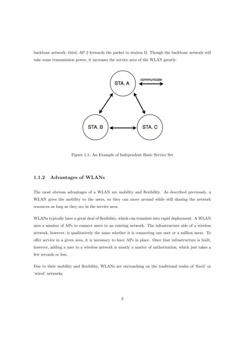
Fig. 1.1 gives a representation of an Independent BSS (IBSS), which is also called an ad-hoc network.

Stations in an IBSS can communicate directly with each other. As shown in Fig. 1.1, stations A, B

and C can transmit packets directly to each other without requiring relaying. The smallest possible

IEEE 802.11 network is an IBSS with two stations. Typically, IBSSs are composed of a small number

of stations set up for a specific purpose and for a short period of time. One common use is to create

a short-lived network to support a single meeting in a conference room. As the meeting begins, the

participants create an IBSS to share data. When the meeting ends, the IBSS is dissolved.

Fig. 1.2 shows an example infrastructure BSS that is common in practice. Infrastructure networks are

distinguished by the use of an AP. APs are used for all communications in infrastructure networks,

including communication between mobile nodes in the same basic service area. Take the case in Fig. 1.2

for instance, if station A needs to communicate with station B, the communication must take two hops:

first, the station A transfers the packet to the AP; second, the AP relays the packet to station B. With

all communications relayed through an AP, the basic service area corresponding to an infrastructure

BSS is defined by the points in which transmissions from the AP can be received. Although multi-hop

transmission takes more transmission power and time than a directed packet transmission from the

sender to the receiver, it has two major advantages. First, an infrastructure BSS is defined by the

distance from the AP. All mobile stations are required to be within reach of the AP, but no restriction

is placed on the distance between mobile stations themselves. Thus a large communication range

is available for infrastructure BSS. Second, allowing direct communication between mobile stations

would save transmission power, but requires them to maintain neighbor relationships with all other

mobile stations within the service area. APs in infrastructure networks are in a position to assist

with stations attempting to save power. APs can note when a station enters a power-saving mode

and buffer packets for it. Battery-operated stations can turn the wireless transceiver off and power it

up only to transmit and retrieve buffered packets from the AP, which can give the battery-operated

stations a longer service time.

BSSs can create coverage in small offices and homes, but they cannot provide network coverage to

larger areas. However, it is possible to link BSSs into an Extended Service Set (ESS). An ESS is

created by chaining BSSs together with a backbone network. As an example, in Fig. 1.3, the ESS

is the union of the BSSs 1 and 2. In each BSS, AP connects to each station wirelessly. AP 1 and

AP 2 are connected by the backbone network, which can be either a wireless or a wired network. In

Fig. 1.3, if station A wants to transmit a packet to station D, the communication must take three

hops: first, the station A transfers the packet to AP 1; second, AP 1 relays the packet to AP 2 by the

2

backbone network; third, AP 2 forwards the packet to station D. Though the backbone network will

take some transmission power, it increases the service area of the WLAN greatly.

Figure 1.1: An Example of Independent Basic Service Set

1.1.2 Advantages of WLANs

The most obvious advantages of a WLAN are mobility and flexibility. As described previously, a

WLAN gives the mobility to the users, so they can move around while still sharing the network

resources as long as they are in the service area.

WLANs typically have a great deal of flexibility, which can translate into rapid deployment. A WLAN

uses a number of APs to connect users to an existing network. The infrastructure side of a wireless

network, however, is qualitatively the same whether it is connecting one user or a million users. To

offer service in a given area, it is necessary to have APs in place. Once that infrastructure is built,

however, adding a user to a wireless network is mostly a matter of authorization, which just takes a

few seconds or less.

Due to their mobility and flexibility, WLANs are encroaching on the traditional realm of ‘fixed’ or

‘wired’ networks.

3

Figure 1.2: An Example of Infrastructure Basic Service Set

Figure 1.3: An Example of Extended Service Set

4

1.2 IEEE 802.11

Since its introduction in 1997, IEEE 802.11 has become the dominant WLAN standard [54]. IEEE

802.11 is a member of the IEEE 802 family, which is a series of specifications for Local Area Network

(LAN) technologies. IEEE 802 specifications are focused on the two lowest layers of the OSI 7-layer

model1, because they incorporate both physical and data link components. All IEEE 802 networks

have both a MAC and a Physical (PHY) component. The MAC layer is a set of rules to determine

how to access the medium and send data, but the details of transmission and reception are left to the

PHY layer.

IEEE 802.11 is a set of standards, which specifies WLAN computer communication in the 2.4 and 5

GHz frequency bands. IEEE 802.11 includes all over-the-air modulation techniques that use the same

basic protocol. The original version of the IEEE 802.11 standard was released in 1997 and clarified

in 1999. It specified two bit-rates of 1 and 2 Mb/s, plus a Forward Error Correction (FEC) code. It

also specified three alternative PHY layer technologies: diffuse InfraRed (IR) operating at 1 Mb/s,

Frequency-Hopping Spread Spectrum (FHSS) operating at 1 Mb/s and 2 Mb/s; and Direct-Sequence

Spread Spectrum (DSSS) at 1 Mb/s and 2 Mb/s. The latter two radio technologies use microwave

transmission over the Industrial Scientific Medical (ISM) frequency band at 2.4 GHz. In this thesis,

we are interested in 5 members in the IEEE 802.11 family, which are IEEE 802.11a, IEEE 802.11b,

IEEE 802.11g, IEEE 802.11e and IEEE 802.11s.

The IEEE 802.11a standard, released in October 1999, uses the same data link layer protocol and

same format as the original IEEE 802.11 protocol, but an Orthogonal Frequency-Division Multiplexing

(OFDM) based air interface at the PHY layer [54]. It operates in the 5 GHz band with a maximum

bit rate of 54 Mb/s. Since the 2.4 GHz band is heavily used to the point of being crowded, using the

relatively lightly used channel of 5 GHz gives IEEE 802.11a some significant advantages. However,

this high carrier frequency also brings some disadvantages. Due to their smaller wavelength, the IEEE

802.11a signals will be absorbed more heavily by walls and other solid objects in their path. As a

result, the IEEE 802.11a signals cannot penetrate as far as those of the IEEE 802.11 b/g that operate

in the frequency band of 2.4 GHz. Consequently, the effective overall range of the IEEE 802.11a rates

is less than that of the IEEE 802.11 b/g rates.

At the same time as the arrival of IEEE 802.11a, IEEE 802.11b was also introduced to the world.

1In the rest of the thesis, we are using the OSI 7-layer model.

5

Similarly, IEEE 802.11b uses the same media method defined in the original standard, but a DSSS

PHY layer technology. IEEE 802.11b adds additional higher bit-rates (5.5 and 11 Mb/s) by adopting

a new modulation scheme named Complementary Code Key (CCK) [54].

IEEE 802.11g, released in June 2003, combines the transmission techniques used by IEEE 802.11a

and IEEE 802.11b, operates at 2.4 GHz and provides all twelve rates originally supported by IEEE

802.11a and IEEE 802.11b [54]. Therefore, IEEE 802.11g supports rates from 1 Mb/s up to 54 Mb/s.

IEEE 802.11e, released in 2005, is an amendment to the original IEEE 802.11 protocol that defines a set

of Quality of Service (QoS) enhancements for WLAN applications through modification to the MAC

layer [54]. This standard is considered of critical importance for delay-sensitive applications, such as

voice over WLAN and streaming multimedia. Thus, IEEE 802.11e divides the network traffic into 4

different categories, according to their delay-sensitivity. By setting different MAC layer parameters,

it allocates different medium access priority to each category.

IEEE 802.11s is a draft IEEE 802.11 amendment for mesh networking, defining how wireless devices

can interconnect to create a WLAN mesh network [54]. A WLAN mesh network is an ESS (as shown

in Fig. 1.3) that has a wireless network as the backbone network. IEEE 802.11s extends the IEEE

802.11 MAC standard by defining an architecture and protocol that support both broadcast/multicast

and unicast delivery using radio-aware metrics over self-configuring multi-hop topologies.

1.2.1 IEEE 802.11 in the MAC Layer

The IEEE 802.11 protocol covers the MAC and PHY layers. The standard currently defines a single

MAC which interacts with three PHYs (IR, FHSS and DSSS). The MAC Layer defines two different

access methods, the Distributed Coordination Function (DCF) and the Point Coordination Function

(PCF).

Distributed Coordination Function

The basic access mechanism, called the DCF, is a Carrier Sense Multiple Access with Collision Avoid-

ance mechanism (CSMA/CA) [119]. A CSMA protocol works as follows. A station with a packet to

transmit senses the medium. If the medium is busy (i.e. any other station is transmitting) then the

6

station postpones its transmission to a later time. If the medium is sensed to be free then the station

transmits.

These kinds of protocols are effective when the medium is not heavily loaded since it allows stations

to transmit with minimum delay. There is, however, always a chance that stations simultaneously

sense the medium as being free and transmit at the same time, which causes a collision.

These collision situations must be identified so the MAC layer can retransmit the packet by itself

and not by upper layers, which would cause significant delay. In an Ethernet network this collision is

sensed by the transmitting stations which go into a retransmission phase based on a binary-exponential

random back-off algorithm.

While these collision detection mechanisms are a good idea for wired LANs, they cannot be used in

a WLAN environment for two main reasons. First, implementing a collision detection mechanism

would require the implementation of a full duplex radio capable of transmitting and receiving at

once, an approach that would increase the price significantly. Second, in a wireless environment

we cannot assume that all stations hear each other, which is the basic assumption of the collision

detection scheme, and the fact that a station wants to transmit and senses the medium as free does

not necessarily mean that the medium is free around the receiver area.

In order to overcome these problems, IEEE 802.11 uses a Collision Avoidance (CA) mechanism to-

gether with a positive acknowledgement scheme [119]. First, a station wanting to transmit senses the

medium. If the medium is busy then it defers the transmission. If the medium is free for a specified

time (called distributed inter frame space, DIFS), then the station is allowed to transmit. Second,

the receiving station checks the integrity of the received packet and sends an acknowledgment packet

(ACK). Receipt of the ACK indicates to the transmitter that no collision occurred. If the sender

does not receive the ACK then it retransmits the packet until it receives an ACK packet. If the

transmission of a packet experiences a number of consecutive failures, the sender should discard this

packet. The re-transmission is governed by a binary exponential back-off algorithm that is described

in detail in Appendix A.

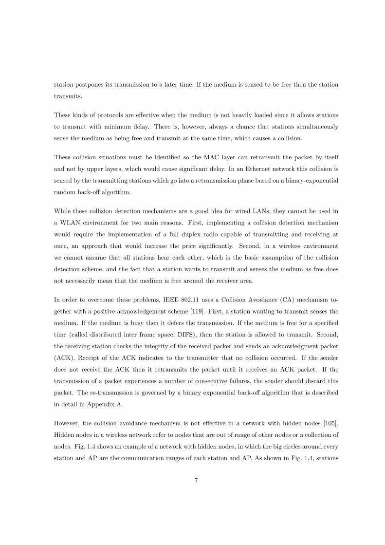
However, the collision avoidance mechanism is not effective in a network with hidden nodes [105].

Hidden nodes in a wireless network refer to nodes that are out of range of other nodes or a collection of

nodes. Fig. 1.4 shows an example of a network with hidden nodes, in which the big circles around every

station and AP are the communication ranges of each station and AP. As shown in Fig. 1.4, stations

7

A and B can communicate with the AP, but they are out of the ranges of each other. Consequently,

when station A is transmitting a packet to the AP, station B can still observe an idle medium and

also transmit a packet to the AP. Therefore, at the AP end, a collision happens, which is called the

hidden node problem. In order to reduce the probability of two stations colliding because of the hidden

node problem, the standard defines a virtual carrier sense mechanism. A station wanting to transmit

a packet first transmits a short control packet called Request To Send (RTS), which includes the

source, destination, and the duration of the following transaction (i.e. the packet and the respective

ACK). The destination station responds (if the medium is free) with a response control packet called

Clear To Send (CTS), which includes the same duration information. All stations receiving either

the RTS and/or the CTS, set their virtual carrier sense indicator (called NAV for Network Allocation

Vector) with the given duration. During this period, these stations must refrained from accessing to

the medium. This mechanism reduces the probability of a collision on the receiver area by a station

that is ‘hidden’ from the transmitter to the short duration of the RTS transaction because the station

hears the CTS and ‘reserves’ the medium as busy until the end of the transmission. The duration

information on the RTS also protects the transmitter area from collisions during the ACK (from

stations that are out of range of the acknowledging station). It should also be noted that, due to the

fact that the RTS and CTS are short frames, the mechanism also reduces the overhead of collisions,

since these are recognized faster than if the whole packet was to be transmitted. This is true if the

packet is significantly bigger than the RTS, so the standard allows for short packets to be transmitted

without the RTS/CTS transaction. This is controlled per station by a parameter called RTS/CTS

threshold.

Point Coordination Function

PCF is an optional access method, which benefits the transmission of time-sensitive information [54].

With PCF, a point coordinator within the AP controls which station can transmit during any given

period of time. Within a time period called the contention free period, the point coordinator will step

through all stations operating in PCF mode and poll them one at a time. For example, the point

coordinator may first poll station A. During a specific period of time station A can then transmit data

frames, while no other station can send anything. The point coordinator then polls the next station

and continues down the polling list, letting each station have a chance to send data. Thus, PCF is a

contention-free protocol and enables stations to transmit data frames synchronously, with regular time

delay between data frame transmissions. This makes it possible to support information flows more

8

Figure 1.4: An Example of a network with hidden nodes

effectively, such as video and control mechanisms that have greater synchronization requirements.

However, PCF is implemented only in very few hardware devices as it is not part of the Wi-Fi

Alliance’s interoperability standard [54].

1.2.2 IEEE 802.11 in the PHY Layer

The modulation techniques and channel coding are the aspects of the PHY layer in which we are

interested in this thesis. The original IEEE 802.11 standard specified DSSS radios that operate at

1 Mb/s and 2 Mb/s in the 2.4GHz frequency band. IEEE 802.11b added additional higher bit-rates

with CCK, and IEEE 802.11g added bit-rates that use OFDM. IEEE 802.11a allows use of frequencies

at 5GHz using only the OFDM bit-rates. Tab. 1.2.2 shows a summary of the modulations and channel

coding for the bit-rates used in IEEE 802.11. Each bit-rate uses some form of FEC with a coding

rate expressed by k/n, where n coded bits are transmitted for every k bits of data. The particular

modulation and coding techniques that bit-rates use are relevant to bit-rate selection because the

techniques use different approaches to increase the capacity of a channel.

9

Rate (Mb/s) Modulation Scheme FEC Rate In IEEE 802.11a/b/g PHY Layer Technology

1 DBPSK 1/11 b/g DSSS

2 DQPSK 1/11 b/g DSSS

5.5 CCK 4/8 b/g DSSS

6 BPSK 1/2 a/g OFDM

9 BPSK 3/4 a/g OFDM

11 CCK 8/8 b/g DSSS

12 QPSK 1/2 a/g OFDM


24 16QAM 1/2 a/g OFDM




Table 1.1: IEEE 802.11a/b/g Transmission Rates

1.3 Main Works

This thesis mainly focuses on the IEEE 802.11 WLANs. In Chapters 2, 3 and 4, we report research

into the DCF mechanism at the MAC layer of the IEEE 802.11. Since analytical models are widely

employed to gain understanding of DCF, due to the low cost and speed with which they can make

predictions, Chapter 2 verifies the fundamental hypotheses shared commonly by many analytical

models. Based on the conclusions obtained in Chapter 2, Chapter 3 builds up an explorative analytical

model without the collision-decoupling hypotheses to find the analytical relationship between the

conditional collision probability and the back-off stage. In Chapter 4, we compare models with or

without the queue-decoupling hypotheses to show the fact that an inappropriate assumption can cause

errors in the predictions.

In the remaining chapters of this thesis, we move our interest to the PHY layer. In Chapter 5, we

experimentally measure the robustness to noise of all IEEE 802.11a/b/g rates, which is important

information for rate control. We find that the robustness to noise is not necessarily a monotonically

decreasing function of the transmission rate, an assumption commonly used in the design of many rate

control algorithms. Bearing this observation in mind, in Chapter 6, we propose a principled design for

10

a rate control algorithm, H-RCA, which is collision-aware and implementable on commodity hardware.

11

Chapter 2

IEEE 802.11 MAC modelling

Hypotheses Testing

2.1 Introduction

Since its introduction in 1997, IEEE 802.11 has become the dominant WLAN standard. One of

its key features is how IEEE 802.11 controls access to the medium, which is based on a Carrier

Sensing Multiple Access / Collision Avoidance (CSMA/CA) algorithm. Due to the widespread use of

IEEE 802.11, considerable research effort has been made to gain understanding of CSMA/CA. This

includes the use of simulation tools, experiments with hardware and the building of analytical models.

Analytical models, in particular, have made great progress in recent years. By October 2010, there

have been over 63,900 articles published related to IEEE 802.11 analytical models according to Google

Scholar.

Despite differences in details of published analytical models, most of them share common hypotheses.

In this chapter, these common hypotheses are identified and investigated. Generally, authors do not

check the validity of these assumptions directly, but infer them from the accuracy of model predictions

of coarse-grained quantities such as long-run throughput. However, if these models are to be used

with confidence for the prediction of quantities beyond those validated within published articles, it is

necessary to ensure the appropriateness of their fundamental hypotheses.

12

In this chapter, the hypotheses are divided into 3 groups according to the type of network model in

which they are employed:

1. hypotheses used for models of general IEEE 802.11 networks;

2. hypotheses used for models of IEEE 802.11e networks;

3. hypotheses used for models of IEEE 802.11s networks.

The work in this chapter was performed in collaboration with Dr. Ken Duffy and Dr. David Malone

(NUIM). Some of these results have been published in [64] and [66].

2.2 Popular Analytical Approaches to IEEE 802.11 DCF and

EDCA

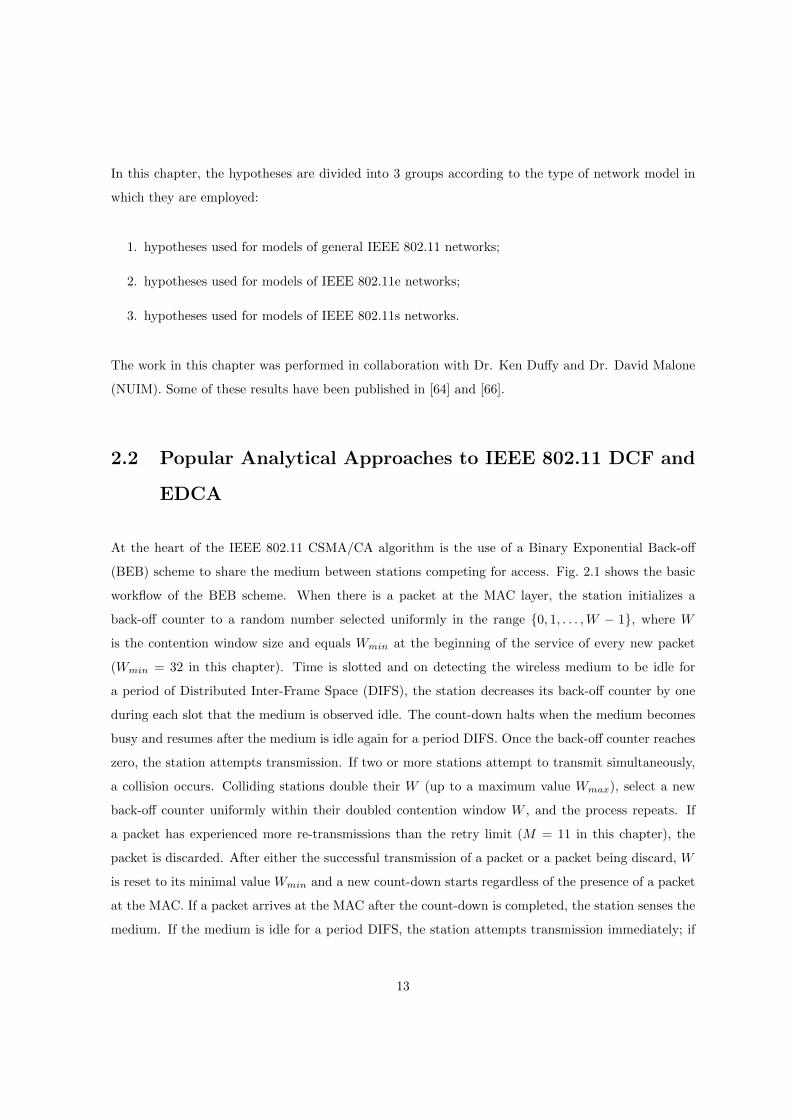
At the heart of the IEEE 802.11 CSMA/CA algorithm is the use of a Binary Exponential Back-off

(BEB) scheme to share the medium between stations competing for access. Fig. 2.1 shows the basic

workflow of the BEB scheme. When there is a packet at the MAC layer, the station initializes a

back-off counter to a random number selected uniformly in the range {0, 1, . . . ,W − 1}, where W

is the contention window size and equals Wmin at the beginning of the service of every new packet

(Wmin = 32 in this chapter). Time is slotted and on detecting the wireless medium to be idle for

a period of Distributed Inter-Frame Space (DIFS), the station decreases its back-off counter by one

during each slot that the medium is observed idle. The count-down halts when the medium becomes

busy and resumes after the medium is idle again for a period DIFS. Once the back-off counter reaches

zero, the station attempts transmission. If two or more stations attempt to transmit simultaneously,

a collision occurs. Colliding stations double their W (up to a maximum value Wmax), select a new

back-off counter uniformly within their doubled contention window W , and the process repeats. If

a packet has experienced more re-transmissions than the retry limit (M = 11 in this chapter), the

packet is discarded. After either the successful transmission of a packet or a packet being discard, W

is reset to its minimal value Wmin and a new count-down starts regardless of the presence of a packet

at the MAC. If a packet arrives at the MAC after the count-down is completed, the station senses the

medium. If the medium is idle for a period DIFS, the station attempts transmission immediately; if

13

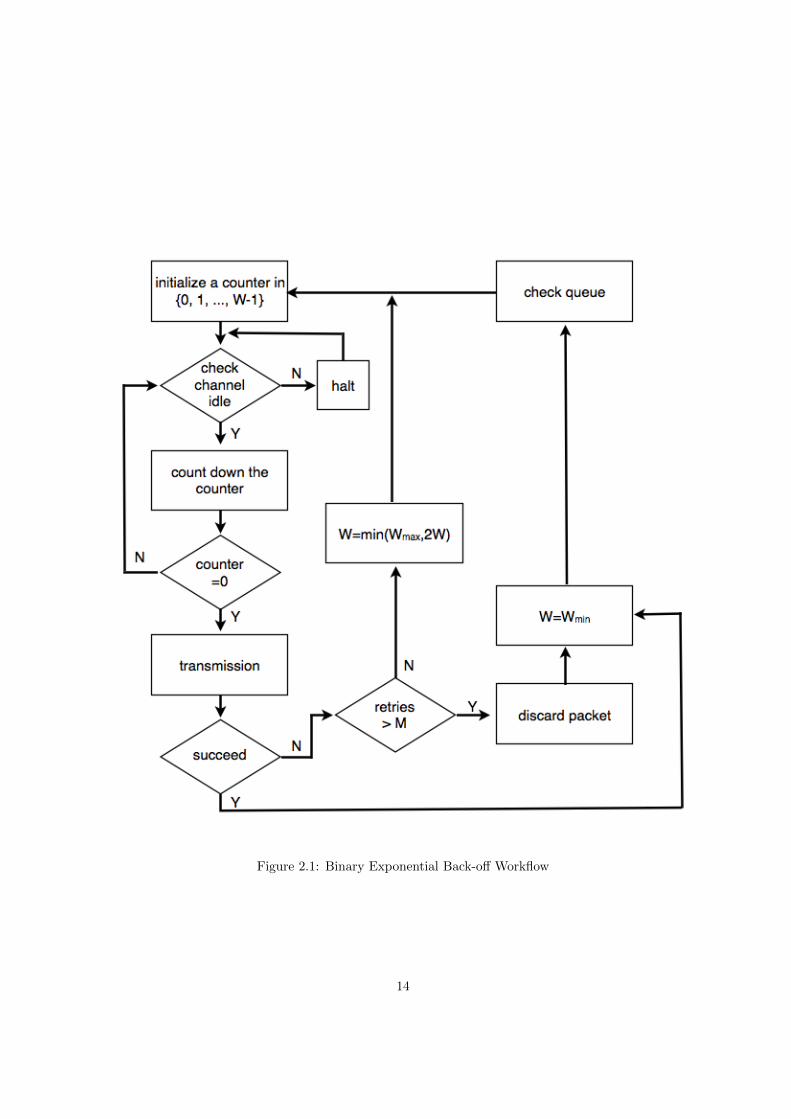
Figure 2.1: Binary Exponential Back-off Workflow

14

it is busy, another back-off counter is uniformly chosen within the initial W . This bandwidth saving

feature is called post-back-off.

In the field of analytical modelling, there are two popular paradigms: the p-persistent approach and

the mean-field Markov model approach. The former has a long history in modelling random access

protocols, such as Ethernet and Aloha [17], and the latter has its foundations in Bianchi’s seminal

papers [18], [19]. While these approaches differ in their ideology and details, we shall see that they

share basic decoupling hypotheses. Irrespective of the paradigm that is adopted, most authors validate

model predictions, but do not directly investigate the veracity of the underlying assumptions.

All of the models we shall consider are based on the assumption of idealized channel conditions

where errors occur only as a consequence of collisions. With this environmental conditioning, the key

decoupling approximation that enables all predictive p-persistent and mean-field analytical models of

the IEEE 802.11 random access MAC is that given a station is attempting transmission, there is a

fixed probability of collision that is independent of the past.

In p-persistent models this arises as each station is assumed to have a fixed probability of attempted

transmission, τ , per idle slot that is independent of the history of the station and independent of all

other stations. In a network of N identical stations, the likelihood a station does not experience a

collision given it is attempting transmission, 1−p, is the likelihood that no other station is attempting

transmission in that slot: 1− p = (1− τ)N−1. Thus the sequence of collisions or successes is an inde-

pendent and identically distributed sequence. In the p-persistent approach, the attempt probability,

τ , is chosen in such a way that the average time to successful transmission matches that in the real

system, which is an input to the model. If this average is known, this methodology has been demon-

strated to make accurate throughput and average delay predictions [31], [32]. One representative of

p-persistent models will be introduced in Chapter 3.

In the mean-field approach, the fundamental idea is similar, but the calculation of τ , and thus p, does

not require external inputs. One starts by assuming that p is given and each station always has a

packet awaiting transmission (the saturated assumption). Then the back-off counter within the station

becomes an embedded, semi-Markov process whose stationary distribution can be determined [18],

[19]. In particular, the stationary probability that the station is attempting transmission, τ(p), can

be evaluated as an explicit function of p and other MAC parameters (Eq. (7) [19]). In a network of N

stations, as τ(p) is known, the fixed point equation 1−p = (1−τ(p))N−1 can be solved to determine the

‘real’ p for the network and ‘real’ attempt probability τ . Once these are known, network performance

15

metrics, such as long run network throughput, can be deduced. A typical example of mean-field

models, a model of unsaturated networks with small buffers, will be introduced in Chapter 4.

Primarily through comparison with simulations and experiments, models based on these assumptions

have been shown to make accurate throughput and delay predictions, even for a small number of

stations. This is, perhaps, surprising as one would expect that the decoupling assumptions would

only be accurate in networks with a large number of stations. The p-persistent paradigm has been

developed to encompass, for example, saturated IEEE 802.11 networks where every station always has

a packet to send [31] and saturated IEEE 802.11e networks [68]. However, due to its intuitive appeal,

its self contained ability to make predictions, and its predictive accuracy, Bianchi’s basic paradigm

has been widely adopted for models that expand on its original range of applicability. A selection

of these extensions include: [8], [45], [48], [92], which consider the impact of unsaturated stations

in the absence of station buffers and enable predictions in the presence of load asymmetries; [33],

[43], [101], [142], which treat unsaturated stations in the presence of stations with buffers; [80], [86],

[111], which investigate the impact of the variable parameters of IEEE 802.11e, including AIFS, on

saturated networks; [34], [39], [47] which treat unsaturated IEEE 802.11e networks; [44], which extends

the paradigm from single hop networks to multiple-radio IEEE 802.11s mesh networks. Note that the

work cited here is a small, selective sub-collection within a vast body of literature. To appreciate just

how large this literature is, as of October 2010, the p-persistent modelling paper [31] has been cited

over 452 times according to ISI Knowledge and over 1,800 times according to Google Scholar, while

the mean-field modelling paper [19] has been cited over 1,576 times according to ISI Knowledge and

over 3,400 times according to Google Scholar.

All of the extensions that we cite are based on the idealized channel assumption, as well as the

decoupling approximation. Some of these extensions require further additional hypotheses.

In this chapter, we use autocovariance, Maximum Likelihood Estimators, Goodness-of-Fit Statistics

(described in Appendix B) and Runs Tests (described in Appendix C) to investigate these fundamental

assumptions with simulation and experimental data.

16

2.3 Hypotheses Used for Models of General IEEE 802.11 Net-

works

2.3.1 Collision-decoupling Hypotheses

As described above, this BEB algorithm couples stations’ service processes through their shared

collisions. Therefore, its performance cannot be analytically investigated without judiciously approx-

imating its behavior. One common decoupling approximation assumes that: whenever a station is

trying to transmit a packet, the probability it will experience a collision is the same, despite of its

transmission history.

For a single station, define Ck := 1 if the kth transmission attempt results in a collision and Ck := 0

if it results in a success. According to the hypothesis above, for a station in an IEEE 802.11 network

employing BEB scheme, irrespective of whether it is saturated (always having packets to send) or not,

the following 2 assumptions should be true:

(A1) The sequence of outcomes of attempted transmissions, {Ck}, forms a stochastically independent

sequence.

(A2) The sequence {Ck} consists of identically distributed random variables that, in particular, do

not depend on past collision history.

These 2 key assumptions in [18], [19], [31], [32] imply that there exists a fixed collision probability

conditioned on attempted transmission, P (Ck = 1) = p, that is assumed to be the same for all back-

off stages and independent of past collisions or successes. Assumptions (A1) and (A2) are common

across all models developed from the p-persistent and mean-field paradigms. Here we investigate

these for saturated stations, for unsaturated stations with small buffers and for unsaturated stations

with big buffers. All network parameters correspond to standard 11 Mb/s IEEE 802.11b [70] and are

summarized in Tab. 2.1.

We begin by investigating (A1), the hypothesized independence of the outcomes (success or collision)

in the sequence of transmission attempts. We draw deductions regarding pairwise independence from

the normalized auto-covariance of the sequence C1, C2, ... , CK(C) obtained in our ns-2 simulations

(as described in Appendix D) and experiments (as described in Appendix E), where K(C) is the

17

Parameters Values

SLOT 20µs

SIFS 10µs

DIFS 50µs

PHYhdr 192bits

Wmin 32

Wmax 1024

Table 2.1: IEEE 802.11b Parameters

Number of stations Saturated Small Buffer Big Buffer

N = 2 6, 638, 246 3, 782, 109 3, 685, 401

N = 5 3, 037, 483 1, 728, 451 1, 508, 178

N = 10 1, 662, 906 937, 708 764, 707

Table 2.2: Numbers of attempted transmissions K(C) in ns-2 simulations.

number of attempted transmissions that a single tagged station has made during the test. For every

simulation and experiment in this sub-section, K(C) is recorded in Tab. 2.2 and Tab. 2.3, respectively.

Assuming {Ck} is wide sense stationary, the normalized auto-covariance, which is a measure of the

pairwise dependence in the sequence, is always 1 at lag 0. If the sequence {Ck} consists of independent

random variables, as hypothesized by (A1), for a sufficiently large sample it would take the value 0 at

all positive lags. Non-zero values correspond to apparent dependencies in the data. In this chapter,

we regard the pairwise dependence as insignificant if the normalized auto-covariance is less than 0.2

by lag 5.

Both simulations and experiments were run for saturated networks with N = 2, 5 & 10, where N is the

Number of stations Saturated Small Buffer Big Buffer

N = 2 2, 549, 550 2, 134, 187 1, 846, 049

N = 5 1, 220, 622 975, 601 749, 295

N = 10 711, 326 502, 955 380, 139

Table 2.3: Numbers of attempted transmissions K(C) in testbed experiments.

18

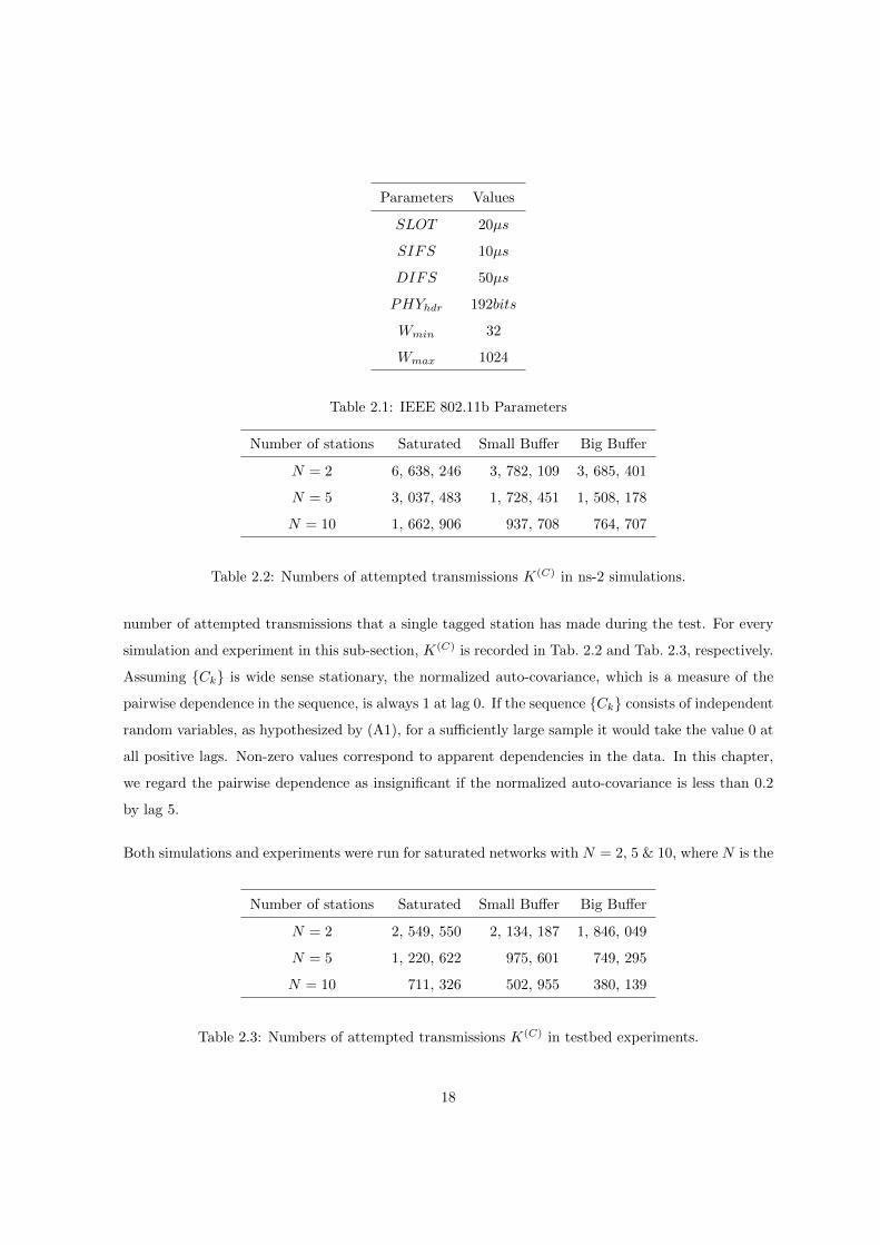
number of stations in the network. As the number of stations increases, the number of transmission

attempts made by the tagged station decreases due to the back-off effect of the MAC. Fig. 2.2 reports

normalized auto-covariances of loss sequences recorded in simulations, while Fig. 2.3 displays the

equivalents in experiments. Both in Fig. 2.2 and 2.3, plots converge to zero quickly (less than 0.2 by

lag 5), which indicates little pairwise dependence in these loss sequences {Ck}, even for N = 2.

0 5 10 15 20−0.02

−0.01

0

0.01

0.02

0.03

0.04

0.05

Lag

Aut

oCov

aria

nce

Coe

ffici

ent

Saturated

N=2N=5N=10

Figure 2.2: Saturated collision sequence normalized auto-covariances. ns-2

Hypothesis (A1) is also adopted in unsaturated models with small buffers [8], [45], [48], [92] and

unsaturated models with big buffers [33], [43], [101], [142]. As in all unsaturated models that we are

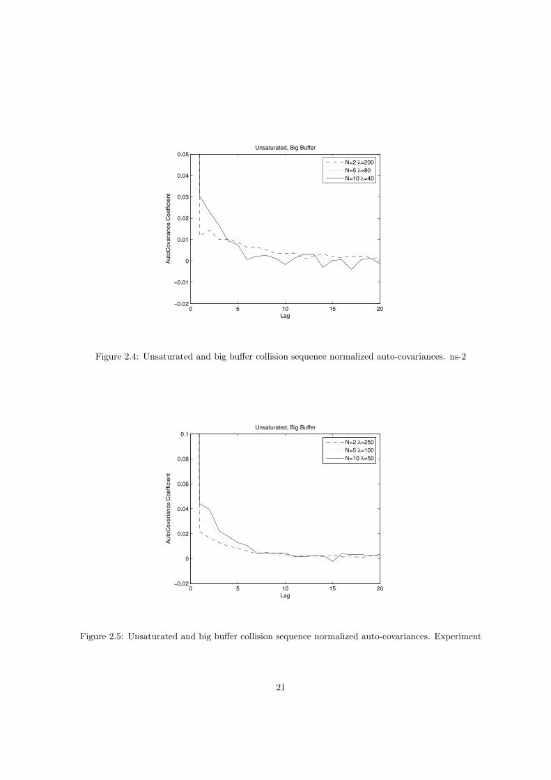
aware of, the traffic for each station is assumed as a Poisson process with rate λ (packets per second).

In both simulation and experiment, the size of packets sent in the network is fixed to 1000 bytes.

In simulations of unsaturated networks with big buffers, the overall network load is kept constant at

400 packets per second, equally distributed amongst the N stations, corresponding to a network-wide

offered load of 3.4 Mb/s. Similarly, the network-wide offered load in experiments is kept constant

at 4.25 Mb/s (500 packets per second). The reason of using different network loads is to gather

information in a wide range and to ensure the universality of this hypotheses testing. Simulation

and experimental results for unsaturated networks with big buffers are shown in Fig. 2.4 and 2.5,

respectively.

Simulation and experimental results for unsaturated networks with small buffers are shown in Fig. 2.6

and 2.7, respectively. The network load in simulations and experiments is kept constant at 4.25 Mb/s

19

0 5 10 15 20−0.1

−0.05

0

0.05

0.1

0.15

0.2

Lag

Aut

oCov

aria

nce

Coe

ffici

ent

Saturated

N=2 λ=750N=5 λ=300N=10 λ=150

Figure 2.3: Saturated collision sequence normalized auto-covariances. Experiment

(500 packets per second) and 6.8 Mb/s (800 packets per second), respectively. Noting the short y-

range in those graphs (Fig. 2.4, 2.5, 2.6 and 2.7), auto-covariances drop to zero beyond small lags (less

than 0.2 by lag 5), which indicates little pairwise dependence in the {Ck} sequences.

Before investigating the (A2) hypothesis on its own, we use the Runs Test (described in Appendix C)

to jointly test (A1) and (A2). Given a binary-valued sequence, C1, . . . , CK(C) this test’s null hypothesis

is that it was generated by a Bernoulli sequence of random variables. The test is non-parametric and

does not depend on P (C1 = 1). In our experimental data, the Runs Tests statistic for each of our

nine collision sequences range from 11.6617 for the saturated, 2-station sequence to 68.5831 for the

unsaturated big-buffer, 2-station sequence. The likelihood that the data was generated by a Bernoulli

sequence is a decreasing function of the test value and if this value is 2.58, there is less than 1%

chance that it was generated by a Bernoulli sequence. Even the lower end of the range gives a p-

value1 of 0, leading to rejection of the hypothesis that the collision sequences are independent and

identically distributed (i.i.d.). The reason for this failure will become apparent when we demonstrate

that P (Ck = 1) depends heavily on an auxiliary variable, αk, the back-off stage at which attempt k

was made and that, as is clear from the DCF algorithm, {αk} cannot form an i.i.d. sequence.

To investigate hypothesis (A2) on its own we reuse the same collision sequence data {Ck} with some

1Given the null hypothesis is true, the p-value is the probability that an event as or more extreme than the test

statistic would be observed; the null hypothesis is rejected if the p-value is small.

20

0 5 10 15 20−0.02

−0.01

0

0.01

0.02

0.03

0.04

0.05

Lag

Auto

Cov

aria

nce

Coe

ffici

ent

Unsaturated, Big Buffer

N=2 !=200N=5 !=80N=10 !=40

Figure 2.4: Unsaturated and big buffer collision sequence normalized auto-covariances. ns-2

0 5 10 15 20−0.02

0

0.02

0.04

0.06

0.08

0.1

Lag

Aut

oCov

aria

nce

Coe

ffici

ent


N=2 λ=250N=5 λ=100N=10 λ=50

Figure 2.5: Unsaturated and big buffer collision sequence normalized auto-covariances. Experiment

21

0 5 10 15 20−0.02

−0.01

0

0.01

0.02

0.03

0.04

0.05

Lag

Aut

oCov

aria

nce

Coe

ffici

ent

Unsaturated, Small Buffer

N=2 λ=250N=5 λ=100N=10 λ=50

Figure 2.6: Unsaturated and small buffer collision sequence normalized auto-covariances. ns-2

0 5 10 15 20−0.02

0

0.02

0.04

0.06

0.08

0.1

Lag

Aut

oCov

aria

nce

Coe

ffici

ent


N=2 λ=400N=5 λ=160N=10 λ=80

Figure 2.7: Unsaturated and small buffer collision sequence normalized auto-covariances. Experiment

22

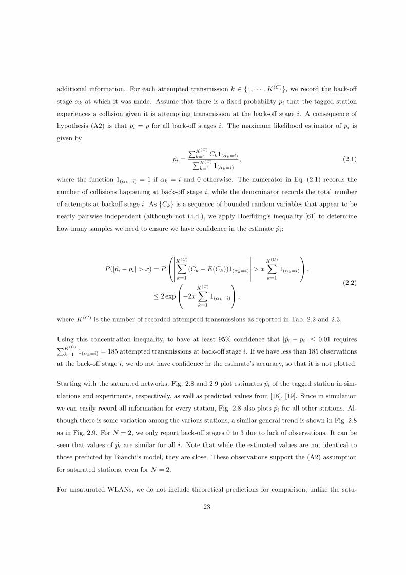
additional information. For each attempted transmission k ∈ {1, · · · ,K(C)}, we record the back-off

stage αk at which it was made. Assume that there is a fixed probability pi that the tagged station

experiences a collision given it is attempting transmission at the back-off stage i. A consequence of

hypothesis (A2) is that pi = p for all back-off stages i. The maximum likelihood estimator of pi is

given by

pi =

∑K(C)

k=1 Ck1(αk=i)∑K(C)

k=1 1(αk=i)

, (2.1)

where the function 1(αk=i) = 1 if αk = i and 0 otherwise. The numerator in Eq. (2.1) records the

number of collisions happening at back-off stage i, while the denominator records the total number

of attempts at backoff stage i. As {Ck} is a sequence of bounded random variables that appear to be

nearly pairwise independent (although not i.i.d.), we apply Hoeffding’s inequality [61] to determine

how many samples we need to ensure we have confidence in the estimate pi:

P (|pi − pi| > x) = P

∣∣∣∣∣∣K(C)∑k=1

(Ck − E(Ck))1(αk=i)

∣∣∣∣∣∣ > x

K(C)∑k=1

1(αk=i)

,

≤ 2 exp

−2x

K(C)∑k=1

1(αk=i)

,

(2.2)

where K(C) is the number of recorded attempted transmissions as reported in Tab. 2.2 and 2.3.

Using this concentration inequality, to have at least 95% confidence that |pi − pi| ≤ 0.01 requires∑K(C)

k=1 1(αk=i) = 185 attempted transmissions at back-off stage i. If we have less than 185 observations

at the back-off stage i, we do not have confidence in the estimate’s accuracy, so that it is not plotted.

Starting with the saturated networks, Fig. 2.8 and 2.9 plot estimates pi of the tagged station in sim-

ulations and experiments, respectively, as well as predicted values from [18], [19]. Since in simulation

we can easily record all information for every station, Fig. 2.8 also plots pi for all other stations. Al-

though there is some variation among the various stations, a similar general trend is shown in Fig. 2.8

as in Fig. 2.9. For N = 2, we only report back-off stages 0 to 3 due to lack of observations. It can be

seen that values of pi are similar for all i. Note that while the estimated values are not identical to

those predicted by Bianchi’s model, they are close. These observations support the (A2) assumption

for saturated stations, even for N = 2.

For unsaturated WLANs, we do not include theoretical predictions for comparison, unlike the satu-

23

−1 0 1 2 3 4 5 6 7 8 9 10 11 12120

0.05

0.1

0.15

0.2

0.25

0.3

0.35

0.4

Backoff Stage

Col

lisio

n P

roba

bilit

y

Saturated

Bianchi N=2NS N=2Bianchi N=5NS N=5Bianchi N=10NS N=10

Figure 2.8: Saturated conditional collision probabilities. ns-2

0 2 4 6 8 10 120

0.05

0.1

0.15

0.2

0.25

0.3

0.35

0.4

0.45

0.5

Backoff Stage

Col

lisio

n P

roba

bilit

y

Saturated

N=2 λ=750N=5 λ=300N=10 λ=150Bianchi

Figure 2.9: Saturated conditional collision probabilities. Experiment

24

−1 0 1 2 3 4 5 6 7 8 9 10 110

0.02

0.04

0.06

0.08

0.1

0.12

0.14

Backoff Stage

Col

lisio

in P

roba

bilit

y


N=2 λ=250N=5 λ=100N=10 λ=50

Figure 2.10: Unsaturated and small buffer conditional collision probabilities. ns-2

rated setting, because there are a large range of distinct models to choose from. Plotting the predic-

tions from any single model would not be particularly informative and could, reasonably, be considered

unfair. The significant thing to note is that all of the models we cite assume that pi = p for all back-off

stages i, so that if pi varies as a function of i, none can provide a perfect match.

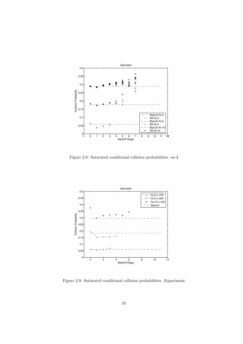
Fig. 2.10 plots estimates pi of each back-off stage i for the tagged station in the unsaturated small

buffer (3 packets space) case with N = 2, 5 & 10, in simulations. Fig. 2.11 plots the equivalent results

from experiments. Noting the small range of the y-axis, these two graphs suggest that hypothesis (A2)

is reasonably appropriate. There is, however, clear pattern in the graphs. For each N , the collision

probability appears to be dependent on the back-off stage. The collision probability at the 1st back-off

stage is higher than at the 0th back-off stage. For stations that are unsaturated, we conjecture that

this occurs as many transmissions happen at back-off stage 0 when no other station has a packet to

send so that collisions are unlikely and p0 is small. Conditioning on the 1st back-off stage is closely

related to conditioning that at least one other station has a packet awaiting transmission, it gives rise

to a higher conditional collision probability at stage 1, so that p1 > p0.

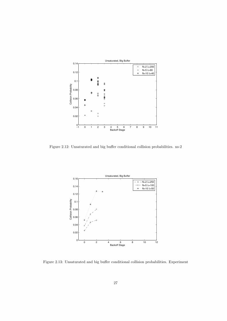
Fig. 2.12 and 2.13 are analogous to Fig. 2.10 and 2.11, but for unsaturated stations with big buffers

(100 packets space). The networks are unsaturated with queues at each station repeatedly emptying.

As with the small buffer case, we again have that p1 > p0 and conjecture that this occurs for the

same reasons. From these 2 graphs, the difference between max(pi) and min(pi) appears to be big,

25

0 2 4 6 8 10 120

0.02

0.04

0.06

0.08

0.1

0.12

0.14

0.16

0.18

Backoff Stage

Col

lisio

n P

roba

bilit

y


N=2 λ=400N=5 λ=160N=10 λ=80

Figure 2.11: Unsaturated and small buffer conditional collision probabilities. Experiment

especially when N = 10. This suggests that (A2) is not a good approximation in the presence of big

station buffers.

As summarized in Tab. 2.5, the pairwise independence of collision sequences {Ck} in saturated and

unsaturated networks is acceptable. The assumption of the identical distribution of variables, Ck, is

only reasonable when networks are saturated or unsaturated with small buffers.

2.3.2 Queue-decoupling Hypotheses

For models where stations have non-zero buffers, it is important to consider the impact of the buffer

when the network is unsaturated. To model stations with buffers serving Poisson traffic, the common

idea across various authors, (e.g. [33], [43], [101], [142]) is to treat each station as a queueing system

where the service time distribution is identified with the MAC delay distribution based on a Bianchi-

like model. The assumptions (A1) and (A2) are adopted, so that given conditional collision probability,

p, each station can be studied on its own and a standard queueing theory model is used to determine

the probability of attempted transmission, τ(p), which is now also a function of the offered load λ.

For symmetrically loaded stations with identical MAC parameters, the network coupling equation,

1− p = (1− τ(p, λ))N−1, identifies the ‘real’ conditional collision probability p.

26

−1 0 1 2 3 4 5 6 7 8 9 10 110

0.02

0.04

0.06

0.08

0.1

0.12

0.14

Backoff Stage

Col

lisio

n P

roba

bilit

y

Unsaturated, BIg Buffer

N=2 λ=200N=5 λ=80N=10 λ=40

Figure 2.12: Unsaturated and big buffer conditional collision probabilities. ns-2

0 2 4 6 8 10 120

0.02

0.04

0.06

0.08

0.1

0.12

0.14

0.16

Backoff Stage

Col

lisio

n P

roba

bilit

y


N=2 λ=250N=5 λ=100N=10 λ=50

Figure 2.13: Unsaturated and big buffer conditional collision probabilities. Experiment

27

Number of stations Big buffer (sim) Big buffer (exp)

N = 2 3, 603, 928 1,799, 250

N = 5 1, 437, 938 720, 044

N = 10 719, 417 359, 413

Table 2.4: Numbers of successful transmissions K(Q).

Each time the MAC successfully transmits a packet, it checks to see if there is another packet in the

buffer awaiting processing. Define Qk := 1 if there is at least one packet awaiting processing after the

kth successful transmission or packet discard, and Qk := 0 if the buffer is empty. As it is technically

challenging to fully model these queueing dynamics while still obtaining tractable equations that can

be solved more quickly than a simulation can be run, authors typically employ a queue-decoupling

assumption that can be distilled into the following two hypotheses:

(A3) The sequence {Qk} consists of independent random variables.

(A4) The sequence {Qk} consists of identically distributed random variables that, in particular, do

not depend on back-off stage.

Defining P (Qk = 1) = q, the value of q is identified with the steady state probability that an associated

M/G/1 or M/G/1/B queueing system has a non-empty buffer after a successful transmission (e.g.

[11]). The M/G/1/B queue is Kendall’s notation [124] for a single-server queue using the first-come

first-served policy where the inter-arrival times are independent and exponentially distributed (M),

the service times are independent and generally distributed (G), and the buffer can hold at most B

packets.

Clearly (A3) and (A4) are more speculative than (A1) and (A2) as both disregard obvious depen-

dencies in the real Q1, . . . , QK(Q) sequence, where K(Q) is the number of successful transmissions

from the tagged station. Values of K(Q) for different network sizes N in simulations and experiments

are summarized in Tab. 2.4. These assumptions are more speculative as if there are two or more

packets awaiting processing after a successful transmission, there will still be another packet awaiting

transmission after the next successful transmission and, in the presence of station buffers, the longer

a packet has been awaiting transmission, the more likely it is to have another packet waiting in its

buffer.

28

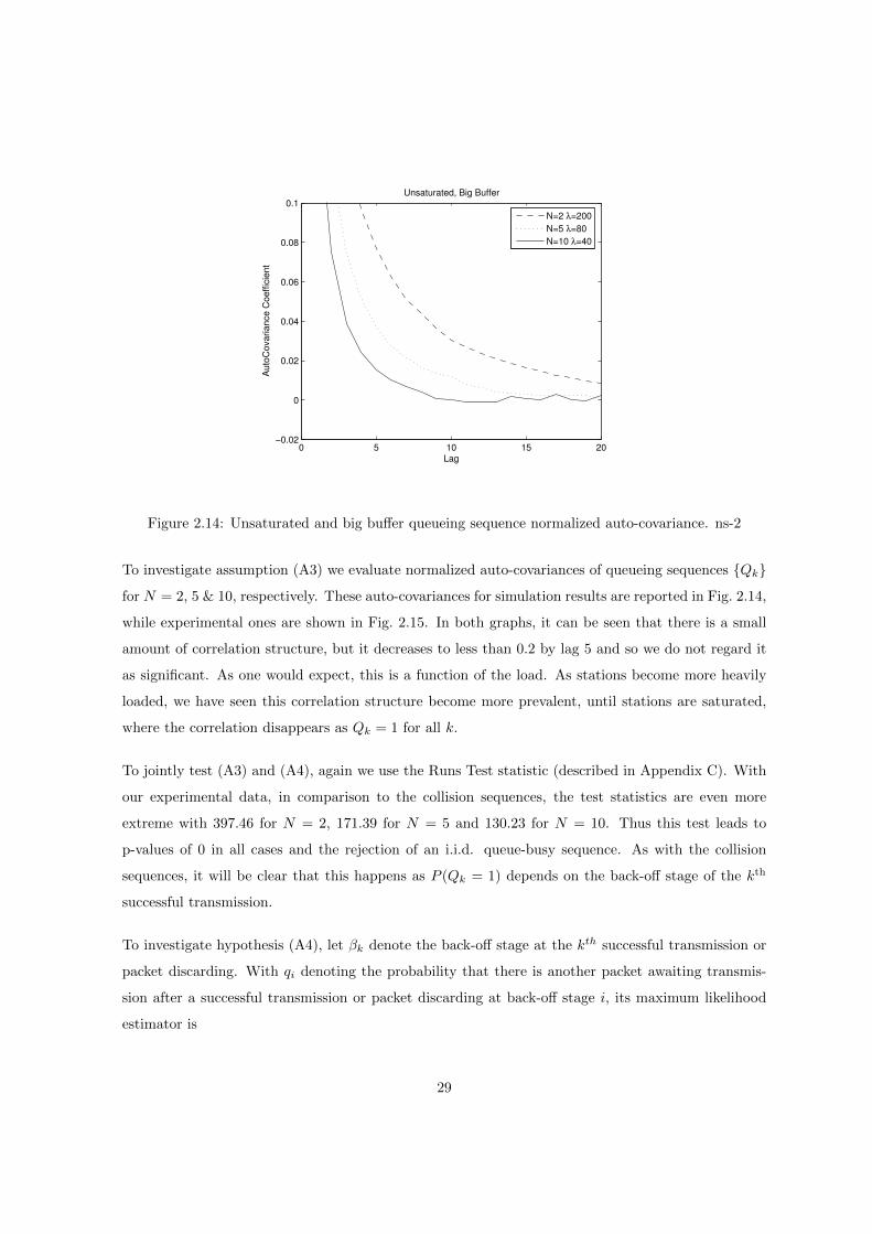
0 5 10 15 20−0.02

0

0.02

0.04

0.06

0.08

0.1

Lag

Aut

oCov

aria

nce

Coe

ffici

ent


N=2 λ=200N=5 λ=80N=10 λ=40

Figure 2.14: Unsaturated and big buffer queueing sequence normalized auto-covariance. ns-2

To investigate assumption (A3) we evaluate normalized auto-covariances of queueing sequences {Qk}

for N = 2, 5 & 10, respectively. These auto-covariances for simulation results are reported in Fig. 2.14,

while experimental ones are shown in Fig. 2.15. In both graphs, it can be seen that there is a small

amount of correlation structure, but it decreases to less than 0.2 by lag 5 and so we do not regard it

as significant. As one would expect, this is a function of the load. As stations become more heavily

loaded, we have seen this correlation structure become more prevalent, until stations are saturated,

where the correlation disappears as Qk = 1 for all k.

To jointly test (A3) and (A4), again we use the Runs Test statistic (described in Appendix C). With

our experimental data, in comparison to the collision sequences, the test statistics are even more

extreme with 397.46 for N = 2, 171.39 for N = 5 and 130.23 for N = 10. Thus this test leads to

p-values of 0 in all cases and the rejection of an i.i.d. queue-busy sequence. As with the collision

sequences, it will be clear that this happens as P (Qk = 1) depends on the back-off stage of the kth

successful transmission.

To investigate hypothesis (A4), let βk denote the back-off stage at the kth successful transmission or

packet discarding. With qi denoting the probability that there is another packet awaiting transmis-

sion after a successful transmission or packet discarding at back-off stage i, its maximum likelihood

estimator is

29

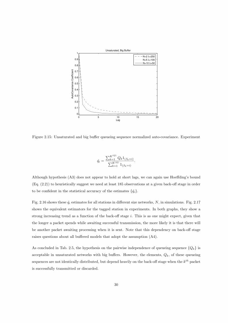
0 5 10 15 200

0.1

0.2

0.3

0.4

0.5

0.6

0.7

0.8

0.9

1

Lag

Aut

oCov

aria

nce

Coe

ffici

ent


N=2 λ=250N=5 λ=100N=10 λ=50

Figure 2.15: Unsaturated and big buffer queueing sequence normalized auto-covariance. Experiment

qi =

∑K(Q)

k=1 Qk1(βk=i)∑K(Q)

k=1 1(βk=i)

.

Although hypothesis (A3) does not appear to hold at short lags, we can again use Hoeffding’s bound

(Eq. (2.2)) to heuristically suggest we need at least 185 observations at a given back-off stage in order

to be confident in the statistical accuracy of the estimates {qi}.

Fig. 2.16 shows these qi estimates for all stations in different size networks, N , in simulations. Fig. 2.17

shows the equivalent estimators for the tagged station in experiments. In both graphs, they show a

strong increasing trend as a function of the back-off stage i. This is as one might expect, given that

the longer a packet spends while awaiting successful transmission, the more likely it is that there will

be another packet awaiting processing when it is sent. Note that this dependency on back-off stage

raises questions about all buffered models that adopt the assumption (A4).

As concluded in Tab. 2.5, the hypothesis on the pairwise independence of queueing sequence {Qk} is

acceptable in unsaturated networks with big buffers. However, the elements, Qk, of these queueing

sequences are not identically distributed, but depend heavily on the back-off stage when the kth packet

is successfully transmitted or discarded.

30

−1 0 1 2 3 4 5 6 7 8 9 10 110

0.1

0.2

0.3

0.4

0.5

0.6

0.7

0.8

0.9

1

Backoff Stage

P(Q

>0)


N=2 λ=250N=5 λ=100N=10 λ=50

Figure 2.16: Unsaturated and big buffer queue-busy probabilities. ns-2

0 2 4 6 8 10 120

0.1

0.2

0.3

0.4

0.5

0.6

0.7

0.8

0.9

Backoff Stage

P(Q

>0)


N=2 λ=250N=5 λ=100N=10 λ=50

Figure 2.17: Unsaturated and big buffer queue-busy probabilities. Experiment

31

Figure 2.18: IEEE 802.11e basic access mechanism

2.4 Hypotheses Used for Models of IEEE 802.11e Networks

The IEEE 802.11e standard, ratified in 2005, enables service differentiation between traffic classes.

Each station is equipped with up to four distinct queues, with each queue effectively being treated

as a distinct station. Each queue has its own MAC parameters including minimum contention win-

dow (Wmin), retry limit (M), transmission opportunity (TXOP ) and arbitration inter-frame space

(AIFS). To model the first three of these, no additional modelling assumptions are necessary beyond

(A1)-(A2) for saturated stations or for unsaturated stations with small buffers (e.g. [92]). For un-

saturated stations with big buffers, no additional assumptions are necessary beyond (A1)-(A4) (e.g.

[43]). However, to capture the full power of IEEE 802.11e’s service differentiation, one must model

AIFS and this requires additional innovation and hypotheses [34], [39], [47], [80], [86], [111].

Fig. 2.18 illustrates the basic access mechanism of IEEE 802.11e. Any station in an IEEE 802.11e

network cannot start its count-down process until it observes the medium being idle as long as AIFS

(called DIFS in IEEE 802.11 a/b/g). Every queue has its associated AIFS = SIFS + AIFSNδ, where

AIFSN ∈ {−1, 0, 1, · · · } and δ is the length of an idle slot. Stations with smaller AIFS can start

their count-down processes first, while stations with bigger AIFS are still waiting. Therefore, stations

with smaller AIFS value will start their count-down processes a few slots ahead of other stations with

bigger AIFS.

Consider N1 + N2 stations, each of which is serving one of two traffic classes with distinct AIFS

values: N1 class 1 stations with AIFS1 and N2 class 2 stations with AIFS2 = AIFS1 + Dδ, where

D is a positive integer. After every attempted transmission, class 1 stations decrease their back-off

counters by a minimum of D before class 2 stations see the medium as being idle. If the back-off

counter of a class 1 stations becomes 0 during these D slots, it attempts transmission and, once it

32

completes, class 1 stations can decrement their counters by at least another D before class 2 stations

see the medium as being idle.

Consider a network of homogeneous saturated class 1 stations and homogeneous class 2 stations. To

model the impact of different AIFS values, using the terminology in [86] we have the notion of hold

states for class 2 stations. A class 2 station is in a hold state if class 1 stations can decrement their

counters while it cannot. As all class 2 stations have the same AIFS value, they all experience the

same class 1 preemption. Once in a hold state, they cannot begin to decrement their back-off counters

again (while class 1 stations continue to do so) unless all class 1 stations are silent for D consecutive

slots.

Given class 2 stations have just entered a hold state, let H ∈ {D,D+ 1, . . . } represent the hold time:

the number of slots that pass before class 2 stations escape the hold states. Let {Hk} denote the

sequence of observations of hold times. Implicitly, the commonly adopted assumptions used to treat

AIFS are:

(A5) The sequence {Hk} consists of independent random variables.

(A6) Each element of the sequence {Hk} is identically distributed, with a distribution that can be

identified with the one described by Eq. (2.3) below.

Within the analytical modelling context, the escape from hold states can be formalized mathematically.

Let τ1 denote the stationary probability a class 1 station attempts transmission. Define Ps1 = (1 −

τ1)N1 , which is the stationary probability that all class 1 stations are silent (no class 1 station is

attempting transmission).

Let {Xn} denote the sequence of hold states. After a transmission, whether successful or not, class

2 stations enter a hold state and this process starts in hold state X0 = 1. If the medium is idle (no

class 1 stations attempt transmission), which happens with probability Ps1 , the station moves to hold

state X1 = 2, otherwise it is reset to X1 = 1, and so forth. The process stops the first time that the

hold state D+ 1 is reached, where all class 2 stations see the medium as being idle and can decrement

their counters. This system forms a Markov chain, portrayed in Fig. 2.19, with the (D+ 1)× (D+ 1)

transition matrix:

33

1

2 D D+1

1

1 3

1−P

sP Ps

s1

1−P

1−P

1−P

P

s

s1

1s

1s

1 1

Figure 2.19: Markov chain for modelling a difference in AIFS of D slots

Π =

1− Ps1 Ps1 0 . . . 0 0

1− Ps1 0 Ps1 . . . 0 0...

......

......

1− Ps1...

... 0 Ps1

0...

... 0 1

.

With X0 = 1, we define H := inf{i : Xi = D + 1} to be the first time that the D consecutive idle

slots are observed. Using the form of the Markov chain, we have

P (H = i) = P (Xi = D + 1)− P (Xi−1 = D + 1)

= (Πi)1,D+1 − (Πi−1)1,D+1.(2.3)

Thus P (H = i) is solely a function of Ps1 and can be readily calculated from Eq. (2.3), albeit not in

closed form unless D = 1 or D = 2.

Due to experimental instrumentation difficulties, the results in this section are based exclusively on

ns-2 simulations. In order to determine how many slots the lower class stations have spent in hold

states, it is necessary to know the start and finish timestamps of every packet transmitted on the

medium. In an experimental setup, no station is in possession of this information and, due to the

time-scales involved, accurate reconciliation of the time-line from data recorded at each station is

particularly challenging. In simulation, however, this data is readily accessible.

34

0 2 4 6 8 10 12 14 16 18 20

0

0.05

0.1

0.15

0.2

0.25

Lag

Auto

Cova

rianc

e Co

effic

ient

D=2D=12D=20D=32

Figure 2.20: Auto-covariances for hold time sequences for class 2 stations in a network of five class 1

and five class 2 saturated stations with D = 2, 12, 20 & 32. ns-2

For a saturated network, the methodology used to measure H is as follows. For each station in the

network, a timestamp is recorded at the start and the end of every transmission. These timestamps

are collected from all stations and combined into a single ordered list: s1, e1, s2, e2, . . . where si is the

start time of the ith packet and ei is the end time. Define Ti := (si+1− ei−AIFS1)/δ for each i ≥ 1.

The hold times are determined from this sequence by first identifying the indices at which the hold

states are delineated: N0 := 0 and Nj+1 := inf{i ≥ Nj : Ti > D} for each i ≥ 1. The hold states are

then the sum of the hold times between transmission, with the final term making a contribution of D

slots:

Hi =

Ni+1−1∑j=Ni+1

Tj +D,

where the empty sum is defined to be zero.

To consider the independence assumption (A5), we assume that the sequence of observed hold times

H1, . . . ,HK(H) are wide sense stationary and plot this data’s auto-covariance function, thus investigat-

ing pairwise dependence. For a network of 5 class 1 saturated stations and 5 class 2 saturated stations

that are identical apart from AIFS2 = AIFS1 +Dδ, where D = 2, 12, 20 & 32, Fig. 2.20 shows their

auto-covariances with K(H) = 1, 717, 545, K(H) = 706, 032, K(H) = 533, 675 and K(H) = 366, 298,

respectively. These plots suggest that these sequences have little dependence at short lags. These

D values, particularly the smaller ones, are typical of those proposed for traffic differentiation in the

35

0 2 4 6 8 10 12 14 160

0.1

0.2

0.3

0.4

0.5

0.6

0.7

0.8

i

P(H

=i)

D=2

SimTheory

Figure 2.21: Empirical and theoretical probability density for the length of a hold period for class 2

stations in a network of five class 1 and five class 2 saturated station with D = 2. ns-2

IEEE 802.11e standard [71]. As the auto-covariance is less than 0.2, the independence assumption

(A5) is reasonable for differences in AIFS values that are proposed in the standard.

To test the assumption (A6), that the probability density of hold times has the form given in Eq. (2.3),

rather than use any specific model prediction for the distribution, as it is a function of single parameter,

Ps1 , we estimate Ps1 based on the following observation. Given D, if the probability that all class 1

stations do not transmit is the same and does not depend on each other, then P (H = D) = Ps1D.

This suggests using the following estimate of Ps1 :∑K(H)

k=1 1(Hk=D)

K(H)

1/D

.

Note that in using this estimate we are ensuring that P (H = D) coincides with the empirical obser-

vation. However, unless the model is accurate, P (H = i) for i 6= D calculated from Eq. (2.3) need

not coincide with the empirically observed value.

Fig. 2.21, 2.22, 2.23 and 2.24 show both empirical and theoretical probability density P (H = i).

Conditioned on having a good estimate of Ps1 , the accuracy of the distribution predicted by Eq. (2.3)

appears to be remarkable. This apparent accuracy can be explored quantitatively through a test

statistic. We use the Kolmogorov-Smirnov test (described in Appendix B), but do not give p-values

36

0 10 20 30 40 50 60 70 80

0

0.05

0.1

0.15

0.2

0.25

0.3

0.35

0.4

i

P(H

=i)

D=12

SimTheory



0 20 40 60 80 100

0

0.05

0.1

0.15

0.2

0.25

0.3

0.35

0.4

0.45

i

P(H=

i)

D=20

SimTheory



37

20 40 60 80 100 120

0

0.05

0.1

0.15

0.2

0.25

0.3

0.35

0.4

i

P(H=

i)

D=32

SimTheory



as our distribution is purely discrete. Fig. 2.25 plots supk |Fn(k) − F (k)| against n for D = 2, 4,

8 &12. It is clear from the graph that the discrepancies are small for moderate values of sample

size. However, supk |Fn(k)− F (k)| is not converging to 0 as n becomes large. This suggests that the

predicted distribution of H is accurate for all practical purposes, even though the distribution is not

a perfect fit.

Therefore, as recorded in Tab. 2.5, these hold time sequences {Hk} are pairwise independent, and

their elements, Hk, are identically distributed with a distribution described by Eq. (2.3).

2.5 Hypotheses Used For Models of IEEE 802.11s Network

The IEEE 802.11s standard is a draft amendment to enable Wireless Mesh Networks (WMNs). One

approach to build a multi-hop, multi-radio mathematical model of a WMN that employs IEEE 802.11s

is to build on the mean-field Markov idea, but with more involved coupling that captures medium

access dependencies across the mesh. In order to do so, it is necessary to make hypotheses about the

stochastic nature of the departures process from mesh points, as these form the arrival processes to

other parts of the mesh.

38

0 2 4 6 8 10

x 104

0

0.01

0.02

0.03

0.04

0.05

0.06

n

sup|

F n(k)−

F(k)

|

D=2D=4D=8D=12

Figure 2.25: Largest discrepancy between empirical and predicted distributions, supk |Fn(k)− F (k)|,

as a function of sample size n. D = 2, 4, 8 & 12. ns-2

Let {Dk} denote the inter-departure times of packets from an element of the network. Thus, Dk is

the difference between the time at which the kth successful transmission and the (k − 1)th successful

transmission occurs from the tagged station. One hypothesis (e.g. [44]) is that if the arrivals process

to the station is Poisson, then the departure process is also Poisson. That is:

(A7) The sequence {Dk} consists of independent random variables.

(A8) The elements of {Dk} are exponentially distributed.

Having observed K(D) inter-departure times, D1, . . . , DK(D) , we investigate these hypotheses. These

inter-departure times were recorded in same experiments as the collision data used in Section 2.3.1, so

that K(D) = K(C) that are reported in Tab. 2.3. Because those simulation results are similar to the

experimental results in this section, only experimental results are shown in this section. Figures 2.26,

2.27 and 2.28 report auto-covariances for saturated arrivals, unsaturated arrivals with small buffers

and unsaturated arrivals with big buffers for networks of N = 2, 5 & 10. There is little dependency

beyond short lags, suggesting that the independence hypothesis (A7) is not inappropriate.

For hypothesis (A8), Fig. 2.29, 2.30 and 2.31 plot the logarithm of one minus the empirical cumula-

tive distribution function of the inter-departure times from the tagged station with big buffer in an

39

0 5 10 15 20−0.1

−0.05

0

0.05

0.1

0.15

0.2

Lag

Aut

oCov

aria

nce

Coe

ffici

ent

Saturated

N=2 λ=750N=5 λ=300N=10 λ=150

Figure 2.26: Saturated inter-departure time sequence normalized auto-covariances. Experiment

0 5 10 15 20−0.1

−0.05

0

0.05

0.1

0.15

0.2

Lag

Aut

oCov

aria

nce

Coe

ffici

ent


N=2 λ=400N=5 λ=160N=10 λ=80

Figure 2.27: Unsaturated and small buffer inter-departure time sequence normalized auto-covariances.

Experiment

40

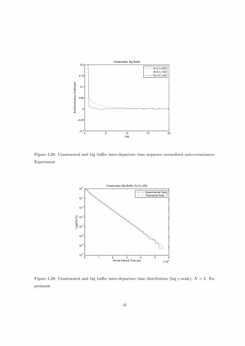
0 5 10 15 20−0.1

−0.05

0

0.05

0.1

0.15

0.2

Lag

Aut

oCov

aria

nce

Coe

ffici

ent


N=2 λ=250N=5 λ=100N=10 λ=50

Figure 2.28: Unsaturated and big buffer inter-departure time sequence normalized auto-covariances.

Experiment

0 1 2 3 4 5 6

x 104

10−7

10−6

10−5

10−4

10−3

10−2

10−1

100

Arrival Interval Time (µs)

Log(

P(t>

T))

Unsaturated, Big Buffer, N=2 λ=250

Experimental DataTheoretical Data

Figure 2.29: Unsaturated and big buffer inter-departure time distribution (log y-scale), N = 2. Ex-

periment

41

0 2 4 6 8 10 12 14x 104

10−6

10−5

10−4

10−3

10−2

10−1

100

Inter−departure Time, t (µs)

P(D

>t)

Unsaturated, Big Buffer, N=5 !=100


Figure 2.30: Unsaturated and big buffer inter-departure time distribution (log y-scale), N = 5. Ex-

periment

0 0.5 1 1.5 2 2.5 3 3.5 4

x 105

10−8

10−7

10−6

10−5

10−4

10−3

10−2

10−1

100


Log(

P(t>

T))

Unsaturated, Big Buffer, N=10 λ=50


Figure 2.31: Unsaturated and big buffer inter-departure time distribution (log y-scale), N = 10.

Experiment

42

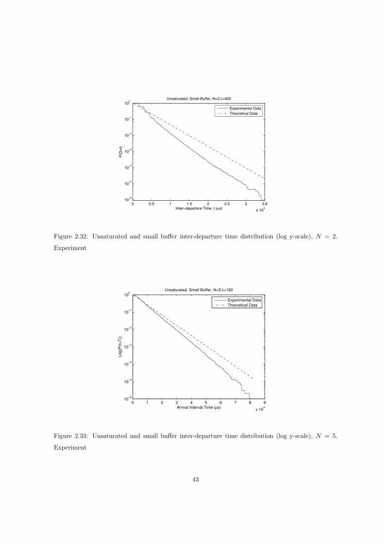
0 0.5 1 1.5 2 2.5 3 3.5x 104

10−6

10−5

10−4

10−3

10−2

10−1

100


P(D

>t)

Unsaturated, Small Buffer, N=2 !=400


Figure 2.32: Unsaturated and small buffer inter-departure time distribution (log y-scale), N = 2.

Experiment

0 1 2 3 4 5 6 7 8 9

x 104

10−6

10−5

10−4

10−3

10−2

10−1

100


Log(

P(t>

T))

Unsaturated, Small Buffer, N=5 λ=160



Experiment

43

0 2 4 6 8 10 12 14 16 18

x 104

10−6

10−5

10−4

10−3

10−2

10−1

100


Log(

P(t>

T))

Unsaturated, Small Buffer, N=10 λ=80



Experiment

0 1 2 3 4 5

x 104

10−7

10−6

10−5

10−4

10−3

10−2

10−1

100


Log(

P(t>

T))

Saturated, N=2 λ=750


Figure 2.35: Saturated inter-departure time distribution (log y-scale), N = 2. Experiment

44

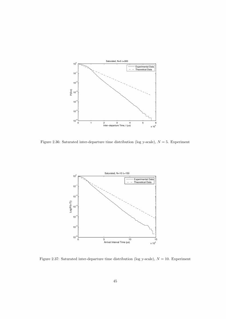
0 1 2 3 4 5 6x 104

10−6

10−5

10−4

10−3

10−2

10−1

100


P(D

>t)

Saturated, N=5 !=300



0 5 10 15

x 104

10−6

10−5

10−4

10−3

10−2

10−1

100


Log(

P(t>

T))

Saturated, N=10 λ=150



45

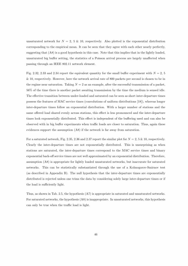
unsaturated network for N = 2, 5 & 10, respectively. Also plotted is the exponential distribution

corresponding to the empirical mean. It can be seen that they agree with each other nearly perfectly,

suggesting that (A8) is a good hypothesis in this case. Note that this implies that in the lightly loaded,

unsaturated big buffer setting, the statistics of a Poisson arrival process are largely unaffected when

passing through an IEEE 802.11 network element.

Fig. 2.32, 2.33 and 2.34 report the equivalent quantity for the small buffer experiment with N = 2, 5

& 10, respectively. However, here the network arrival rate of 800 packets per second is chosen to be in

the regime near saturation. Taking N = 2 as an example, after the successful transmission of a packet,

56% of the time there is another packet awaiting transmission by the time the medium is sensed idle.

The effective transition between under-loaded and saturated can be seen as short inter-departure times

possess the features of MAC service times (convolutions of uniform distributions [18]), whereas longer

inter-departure times follow an exponential distribution. With a larger number of stations and the

same offered load shared evenly across stations, this effect is less pronounced and the inter-departure

times look exponentially distributed. This effect is independent of the buffering used and can also be

observed with in big buffer experiments when traffic loads are closer to saturation. Thus, again these

evidences support the assumption (A8) if the network is far away from saturation.

For a saturated network, Fig. 2.35, 2.36 and 2.37 report the similar plot for N = 2, 5 & 10, respectively.

Clearly the inter-departure times are not exponentially distributed. This is unsurprising as when

stations are saturated, the inter-departure times correspond to the MAC service times and binary

exponential back-off service times are not well approximated by an exponential distribution. Therefore,

assumption (A8) is appropriate for lightly loaded unsaturated networks, but inaccurate for saturated

networks. This can be statistically substantiated through the use of a Kolmogorov-Smirnov test

(as described in Appendix B). The null hypothesis that the inter-departure times are exponentially

distributed is rejected unless one trims the data by considering solely large inter-departure times or if

the load is sufficiently light.

Thus, as shown in Tab. 2.5, the hypothesis (A7) is appropriate in saturated and unsaturated networks.

For saturated networks, the hypothesis (A8) is inappropriate. In unsaturated networks, this hypothesis

can only be true when the traffic load is light.

46

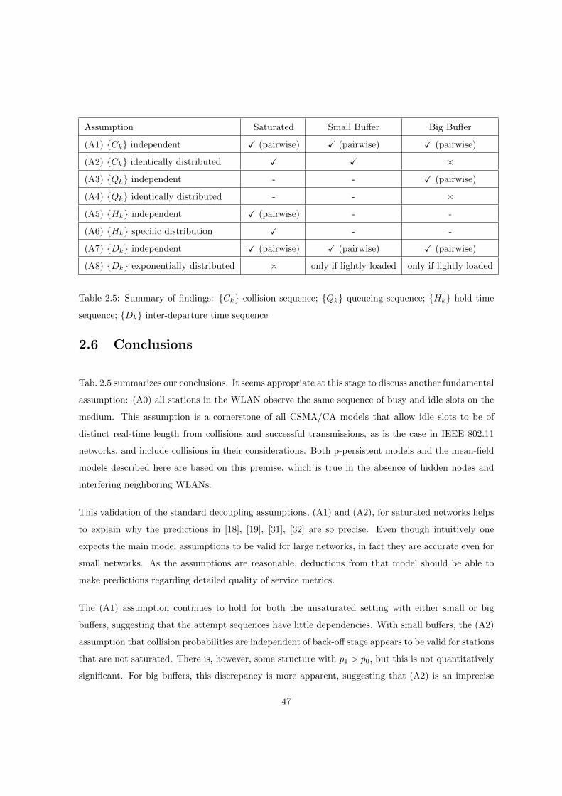
Assumption Saturated Small Buffer Big Buffer

(A1) {Ck} independent X (pairwise) X (pairwise) X (pairwise)

(A2) {Ck} identically distributed X X ×

(A3) {Qk} independent - - X (pairwise)

(A4) {Qk} identically distributed - - ×

(A5) {Hk} independent X (pairwise) - -

(A6) {Hk} specific distribution X - -

(A7) {Dk} independent X (pairwise) X (pairwise) X (pairwise)

(A8) {Dk} exponentially distributed × only if lightly loaded only if lightly loaded

Table 2.5: Summary of findings: {Ck} collision sequence; {Qk} queueing sequence; {Hk} hold time

sequence; {Dk} inter-departure time sequence

2.6 Conclusions

Tab. 2.5 summarizes our conclusions. It seems appropriate at this stage to discuss another fundamental

assumption: (A0) all stations in the WLAN observe the same sequence of busy and idle slots on the

medium. This assumption is a cornerstone of all CSMA/CA models that allow idle slots to be of

distinct real-time length from collisions and successful transmissions, as is the case in IEEE 802.11

networks, and include collisions in their considerations. Both p-persistent models and the mean-field

models described here are based on this premise, which is true in the absence of hidden nodes and

interfering neighboring WLANs.

This validation of the standard decoupling assumptions, (A1) and (A2), for saturated networks helps

to explain why the predictions in [18], [19], [31], [32] are so precise. Even though intuitively one

expects the main model assumptions to be valid for large networks, in fact they are accurate even for

small networks. As the assumptions are reasonable, deductions from that model should be able to

make predictions regarding detailed quality of service metrics.

The (A1) assumption continues to hold for both the unsaturated setting with either small or big

buffers, suggesting that the attempt sequences have little dependencies. With small buffers, the (A2)

assumption that collision probabilities are independent of back-off stage appears to be valid for stations

that are not saturated. There is, however, some structure with p1 > p0, but this is not quantitatively

significant. For big buffers, this discrepancy is more apparent, suggesting that (A2) is an imprecise

47

approximation in that setting. For big buffer models, this inaccuracy is less dramatic than the failure

of the additional queue-decoupling assumption (A3) and (A4).

Our investigations indicate that while (A3) is reasonable at lighter loads, neither (A3) or (A4) are

appropriate in general. In particular, contradicting (A4), the probability that the queue is non-

empty after a successful transmission is strongly dependent on back-off stage. Despite the apparent

inappropriateness of the assumptions (A3) and (A4), models based on them continue to make accurate

predictions of goodput and average delay. One explanation is that with an infinite buffer, unless

the station is saturated, the goodput corresponds to the offered load. Thus, to have an accurate

goodput model it is only important that the model be accurate when offered load leads a station to

be nearly saturated. Once saturated, (A4) is true as Bianchi’s model is recovered. Thus, for goodput,

the inaccuracy of the approximation (A4) is not significant if this phase transition is predicted by

the model. Another possible reason is that most of models only give predictions for homogeneous

symmetric networks, which may hide the inappropriateness of (A4). As evidence, in Chapter 4,

we have shown (A4) leads to inaccurate predictions for throughput of stations in a network with

asymmetric payload. Therefore, one would expect that for more subtle quantities the adoption of

(A4) would lead to erroneous deductions. Clearly caution must be taken when making deductions

from big buffer models that incorporate these hypotheses. Extrapolations of that kind from these

models should be made with care by network designers.

The hold state hypotheses that were introduced to incorporate IEEE 802.11e AIFS differentiation

in saturated networks are labeled (A5) and (A6). The independence hypothesis (A5) appears to be

appropriate. The distributional assumption (A6) appears to be accurate for any difference in AIFS

once one has a good estimate of the probability that no higher class station attempts transmission

in a typical slot. This lends confidence to the use of these models for network design and detailed

predictions.

The IEEE 802.11s mesh network assumptions (A7) and (A8) hold true for lightly loaded, unsaturated

networks, where stations can have either large or small buffers. In particular, the output of an

unsaturated IEEE 802.11 station with Poisson arrivals again appears to be nearly Poisson, so long

as the network is far away from saturation. However, if the station is close to saturation, the inter-

departure times correspond to MAC delays, which do not follow an exponential distribution. If

stations are close to being saturated, short inter-departure times are similar to MAC delays, whereas

long inter-departure times correspond to long inter-arrival times and are Poissonian. The impact of

48

this non-Poisson traffic on the accuracy of unsaturated model predictions must be investigated before

they can be used with confidence.

We also make a comment regarding experimentation. It was challenging to emulate the fundamental

explicit hypothesis of all the models that we investigated: that of idealized channel conditions where

errors occur only as a consequence of collisions. As IEEE 802.11 operates in an unlicensed range of the

spectrum and other devices are free to operate in this range, these devices lead to interference. There

are extensions to the WLAN modelling paradigms that include failed transmissions due to noise on the

medium, e.g. [100]. This approach assumes that packet losses due to noise are i.i.d. and independent

of all other stochastic processes in the model. Whether this assumption is appropriate is dependent

on the particular environment at hand and, clearly, cannot be subject to general validation.

Due to the failure of several of these fundamental hypotheses, clearly there is more work to be done

on analytical modelling of IEEE 802.11. In particular, models that incorporate buffers at stations

are based on flawed hypotheses, but are important for network designers. We suggest that it is an

important challenge for the analytical modelling community to revisit and revise models based on

these inappropriate assumptions.

49

Chapter 3

An Explorative Model for

Conditional Collision Probability

3.1 Introduction

As described in Chapter 2, all p-persistent and mean-field analytical models of the IEEE 802.11

random access MAC are based on the collision-decoupling hypotheses. For the tagged station in a

network, define Ck := 1 if its kth transmission attempt results in a collision, and Ck := 0 otherwise.

The collision-decoupling hypotheses are distilled into the following hypotheses:

(A1) The sequence of outcomes of attempted transmissions, {Ck}, forms a stochastically independent

sequence;

(A2) The sequence {Ck} consists of identically distributed random variables that, in particular, do

not depend on past collision history.

In Section 2.3.1, these hypotheses are shown to be approximately appropriate in saturated networks

and unsaturated networks with small buffers, even when the number of stations in a network is as low

as 2.

50

Fig. 3.1, 3.2 and 3.3 display the estimated conditional collision probabilities derived from our ns-

2 simulation data for saturated networks, unsaturated networks with big buffers and unsaturated

networks with small buffers, respectively, obtained in Section 2.3.1. In these simulations, we assume

the payload traffic follows a Poisson process with incoming rate, λ (packets per second), and the

packet size is 1000 bytes. In each graph, despite the size of these networks, N , the conditional

collision probabilities pi share a similar trend. In the saturated networks (Fig. 3.1), pi decreases when

the station moves to the back-off stage 1 from the back-off stage 0, and then increases when the station

is at the higher back-off stages. Unlike the saturated networks, in the unsaturated networks (Fig. 3.2

and 3.3), pi increases when the station gets into the back-off stage 1 from the back-off stage 0, and

then decreases as the station moves to the higher back-off stages. For these phenomena, Chapter

2 gives plausible, but heuristic explanations. For the observation that p0 < p1 in the unsaturated

networks, we conjecture that this occurs as many transmissions happen at back-off stage 0 when no

other station has a packet to send so that collisions are unlikely and p0 is small; conditioning on the

1st back-off stage is closely related to conditioning that at least one other station has a packet awaiting

transmission, and it gives rise to a higher conditional collision probability at back-off stage 1. In this

chapter, our goal is to obtain analytical explanations for these phenomena.

In this chapter, using the collision-decoupling hypothesis (A1), but avoiding the collision-decoupling

hypothesis (A2), we build up an explorative model that enables us to rigorously substantiate the

intuitive explanation for the relationship between conditional collision probabilities and their corre-

sponding back-off stages. We will introduce our model in Section 3.2, and display results in Section

3.3. This chapter is summarized in Section 3.4.

3.2 Explorative Model

As the background knowledge for this chapter, IEEE 802.11’s Distributed Coordination Function

(DCF) algorithm is introduced in Appendix A. In this chapter, we still assume the collision sequence

{Ck} consists of independent random variables (A1), but abandon the assumption that the elements

in this sequence are identically distributed (A2). The independence assumption on {Ck} has been

verified in Section 2.3.1. Instead of decoupling the behavior of a whole network into the behavior of

individual stations in this network, we analyze behaviors of all stations in the network together. The

complexity of the model increases exponentially as the the size of the network, N , increases. Therefore,

51

−1 0 1 2 3 4 5 6 7 8 9 10 11 12120

0.05

0.1

0.15

0.2

0.25

0.3

0.35

0.4

Backoff Stage

Col

lisio

n Pr

obab

ility

Saturated

Bianchi N=2NS N=2Bianchi N=5NS N=5Bianchi N=10NS N=10

Figure 3.1: Conditional Collision Probability of Saturated Networks. ns-2

−1 0 1 2 3 4 5 6 7 8 9 10 110

0.02

0.04

0.06

0.08

0.1

0.12

0.14

Backoff Stage

Col

lisio

n Pr

obab

ility

Unsaturated, BIg Buffer

N=2 !=200N=5 !=80N=10 !=40

Figure 3.2: Conditional Collision Probability of Unsaturated Networks with Big Buffers. ns-2

52

−1 0 1 2 3 4 5 6 7 8 9 10 110

0.02

0.04

0.06

0.08

0.1

0.12

0.14

Backoff Stage

Col

lisio

in P

roba

bilit

y


N=2 λ=250N=5 λ=100N=10 λ=50

Figure 3.3: Conditional Collision Probability of Unsaturated Networks with Small Buffers. ns-2

to make our explorative model mathematically tractable, we must make several restrictions on the

network model. First, the number of stations in the network is restricted to N = 2. To avoid

the queue-decoupling hypotheses ((A3) and (A4) in Section 2.3.2), we assume both stations have

no buffer. In each station, the highest back-off stage is 2, and the maximum contention window is

Wmax = 22Wmin with the minimum contention window Wmin = 32. In our model, we assume there

is no retry limit, M = ∞. Therefore, when the station experiences a collision at the back-off stage

2, the station stays at the back-off stage 2 until it transmits this packet successfully. We assume the

incoming traffic follows a Poisson process with incoming rate λ (packets per second). Time is slotted

in this model. In every busy or idle slot, depending on the current back-off stage i of the station, each

station has a fixed probability, τi, to make a transmission attempt. Although this simplified network

model is small in the numbers of stations and back-off stages, as an explorative model, it still exhibits

many interesting features of the IEEE 802.11’s DCF algorithm, especially the analytical relationship

between the conditional collision probability and the back-off stage.

Let the sequence {αk} record the back-off stage i at which the kth transmission attempt is made.

Instead of assuming the collision sequence {Ck} consists of independent and identically distributed

(i.i.d.) random variables, we assume the elements in the subsequence {Ck|αk} are i.i.d. Thus, we

define the conditional collision probability at the back-off stage i, pi, as:

pi := P (Ck = 1|αk = i).

53

At the kth slot, for a single station, define Ok := 1 if the station attempts to transmit at the kth

slot, and Ok := 0 if not. We assume the resulting transmission sequence {Ok} consists of independent

random variables, and the transmission sequences {Ok} of stations 1 and 2 are independent of each

other. Indicate γk as the current back-off stage of the station at the kth slot. We assume the

subsequences {Ok|γk = i} are i.i.d. Given the current back-off stage is i, the conditional transmission

probability, τi, is defined as:

τi := P (Ok = 1|γk = i).

Since there is no buffer at each station, each station will wait for a new packet after it transmits its

current packet successfully. In our model, in addition to the back-off stages 0, 1 and 2, we introduce

an idle stage. Thus, after the tagged station finishes the service of its current packet, instead of going

back to the back-off stage 0, it enters the idle stage and stays there until a new packet arrives. As the

incoming traffic is assumed to follow a Poisson process with incoming rate λ (packets per second), let

r be the probability that at least one packet arrives during an average slot when the tagged station is

waiting for a new packet, which has the following expression:

r = 1−((1− τ)2 exp(−λδ) +

(1− (1− τ)2

)exp(−λTb)

), (3.1)

where δ and Tb are the length of the idle or busy slot, respectively. In Eq. (3.1), (1 − τ)2 is the

probability that no station transmits in this slot (an idle slot), while exp(−λδ) and exp(−λTb) are the

probabilities that no packet arrives in this idle or busy slot, respectively.

In the kth slot, let Xk = (i, j) where i, j ∈ {idle, 0, 1, 2} are the current stages of stations 1 and 2,

respectively. As we assume that the collision sequences {Ck = 1|αk = i} consist of i.i.d. random

variables and the incoming traffic follows a Poisson process, we have:

P (Xk+1 = (ik+1, jk+1)|Xk = (ik, jk), · · · , X1 = (i1, j1)) = P (Xk+1 = (ik+1, jk+1)|Xk = (ik, jk)),

where ik, jk ∈ {idle, 0, 1, 2} for all k. Therefore, the sequence {Xk} has the Markov property and

forms a Markov chain.

When Xk = (idle, idle), each station can enter the back-off stage 0 in the next slot if and only if it has

a new packet arriving. Thus, we have:

P (Xk+1 = (idle, idle)|Xk = (idle, idle)) = (1− r)2;

P (Xk+1 = (0, idle)|Xk = (idle, idle)) = P (Xk+1 = (idle, 0)|Xk = (idle, idle)) = r(1− r);

P (Xk+1 = (0, 0)|Xk = (idle, idle)) = r2.

54

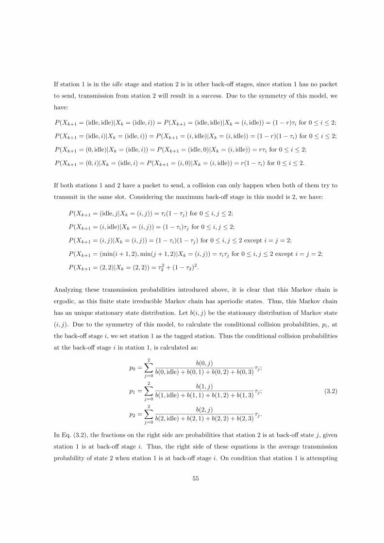
If station 1 is in the idle stage and station 2 is in other back-off stages, since station 1 has no packet

to send, transmission from station 2 will result in a success. Due to the symmetry of this model, we

have:

P (Xk+1 = (idle, idle)|Xk = (idle, i)) = P (Xk+1 = (idle, idle)|Xk = (i, idle)) = (1− r)τi for 0 ≤ i ≤ 2;

P (Xk+1 = (idle, i)|Xk = (idle, i)) = P (Xk+1 = (i, idle)|Xk = (i, idle)) = (1− r)(1− τi) for 0 ≤ i ≤ 2;

P (Xk+1 = (0, idle)|Xk = (idle, i)) = P (Xk+1 = (idle, 0)|Xk = (i, idle)) = rτi for 0 ≤ i ≤ 2;

P (Xk+1 = (0, i)|Xk = (idle, i) = P (Xk+1 = (i, 0)|Xk = (i, idle)) = r(1− τi) for 0 ≤ i ≤ 2.

If both stations 1 and 2 have a packet to send, a collision can only happen when both of them try to

transmit in the same slot. Considering the maximum back-off stage in this model is 2, we have:

P (Xk+1 = (idle, j|Xk = (i, j)) = τi(1− τj) for 0 ≤ i, j ≤ 2;

P (Xk+1 = (i, idle)|Xk = (i, j)) = (1− τi)τj for 0 ≤ i, j ≤ 2;

P (Xk+1 = (i, j)|Xk = (i, j)) = (1− τi)(1− τj) for 0 ≤ i, j ≤ 2 except i = j = 2;

P (Xk+1 = (min(i+ 1, 2),min(j + 1, 2)|Xk = (i, j)) = τiτj for 0 ≤ i, j ≤ 2 except i = j = 2;

P (Xk+1 = (2, 2)|Xk = (2, 2)) = τ22 + (1− τ2)2.

Analyzing these transmission probabilities introduced above, it is clear that this Markov chain is

ergodic, as this finite state irreducible Markov chain has aperiodic states. Thus, this Markov chain

has an unique stationary state distribution. Let b(i, j) be the stationary distribution of Markov state

(i, j). Due to the symmetry of this model, to calculate the conditional collision probabilities, pi, at

the back-off stage i, we set station 1 as the tagged station. Thus the conditional collision probabilities

at the back-off stage i in station 1, is calculated as:

p0 =

2∑j=0

b(0, j)

b(0, idle) + b(0, 1) + b(0, 2) + b(0, 3)τj ;

p1 =

2∑j=0

b(1, j)

b(1, idle) + b(1, 1) + b(1, 2) + b(1, 3)τj ;

p2 =

2∑j=0

b(2, j)

b(2, idle) + b(2, 1) + b(2, 2) + b(2, 3)τj .

(3.2)

In Eq. (3.2), the fractions on the right side are probabilities that station 2 is at back-off state j, given

station 1 is at back-off stage i. Thus, the right side of these equations is the average transmission

probability of state 2 when station 1 is at back-off stage i. On condition that station 1 is attempting

55

transmission, the right side of the above equations is also the conditional collision probability pi for

station 1.

Since the number of stations in this model is N = 2, when a station is attempting transmission, it

can experience a collision only when the other station transmits at the same time. Thus, the average

conditional collision probability, p, equals the average transmission rate, τ :

p = τ =

2∑i=0

(b(0, i) + b(1, i) + b(2, i)) τi, (3.3)

where the sum in the brackets is the stationary probability that station 2 is in the back-off stage i.

Eq. (3.2) and Eq. (3.3) are functions of the conditional transmission probabilities τi and the arrival

probability r. As defined in IEEE 802.11 protocol [120], with a packet in the MAC layer, at the back-off

stage i, an integer back-off counter, g, is chosen randomly and uniformly in {0, 1, 2, · · · ,Wi − 1}, and

the station can only transmit the packet when the back-off counter reduces to 0. Therefore, the back-off

waiting times at the back-off stage i are independent and uniformly distributed in {0, 1, 2, · · · ,Wi−1}.

Considering the station takes 1 slot to transmit the packet, the average service time, Di, at the back-off

stage i (for 0 ≤ i ≤ 2) is given by:

Di =

Wi−1∑j=0

1

Wij + 1 =

Wi + 1

2for 0 ≤ i ≤ 2.

Since we assume the elements in the subsequence {Ok|γk = i} are i.i.d. with P (Ok = 1|γk = i) = τi,

the subsequence {Ok|γk = i} forms a Bernoulli process. Thus, the service time at the back-off stage

i has a geometric distribution with probability τi. Therefore, the average service time, Di, at the

back-off stage i (for 0 ≤ i ≤ 2) also equals 1/τi. As a result, we have:

τi =1

Di=

2

Wi + 1for 0 ≤ i ≤ 2.

Therefore, Eq. (3.2) and Eq. (3.3) can be rewritten as functions of the arrival probability r. It is

clear that Eq. (3.1) and Eq. (3.3) make up a fixed point equation that determines the value of the

arriving probability r with a given incoming rate λ. Thus, given an incoming rate λ, the values of

the conditional collision probabilities, pi, and the average conditional collision probability, p, can be

derived from Eq. (3.1), (3.2) and (3.3).

56

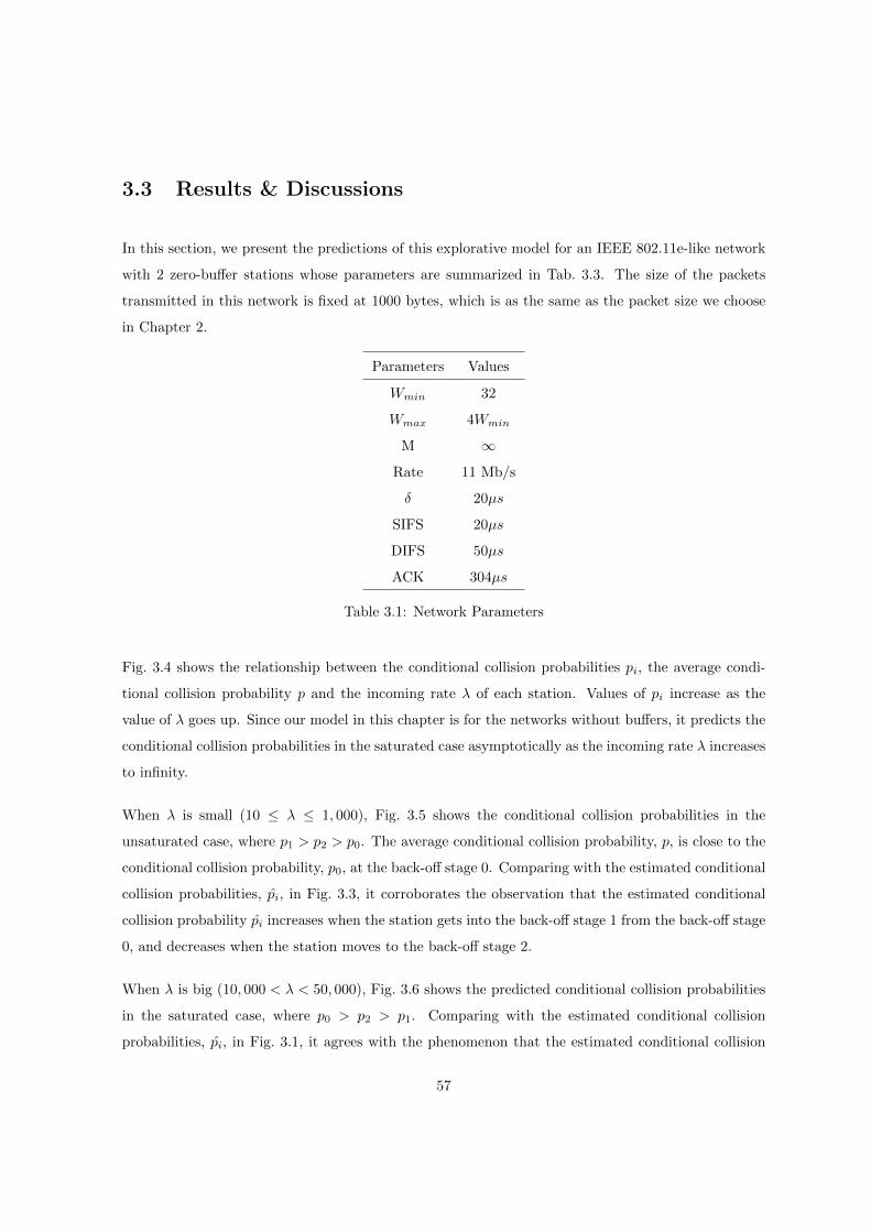
3.3 Results & Discussions

In this section, we present the predictions of this explorative model for an IEEE 802.11e-like network

with 2 zero-buffer stations whose parameters are summarized in Tab. 3.3. The size of the packets

transmitted in this network is fixed at 1000 bytes, which is as the same as the packet size we choose

in Chapter 2.

Parameters Values

Wmin 32

Wmax 4Wmin

M ∞

Rate 11 Mb/s

δ 20µs

SIFS 20µs

DIFS 50µs

ACK 304µs

Table 3.1: Network Parameters

Fig. 3.4 shows the relationship between the conditional collision probabilities pi, the average condi-

tional collision probability p and the incoming rate λ of each station. Values of pi increase as the

value of λ goes up. Since our model in this chapter is for the networks without buffers, it predicts the

conditional collision probabilities in the saturated case asymptotically as the incoming rate λ increases

to infinity.

When λ is small (10 ≤ λ ≤ 1, 000), Fig. 3.5 shows the conditional collision probabilities in the

unsaturated case, where p1 > p2 > p0. The average conditional collision probability, p, is close to the

conditional collision probability, p0, at the back-off stage 0. Comparing with the estimated conditional

collision probabilities, pi, in Fig. 3.3, it corroborates the observation that the estimated conditional

collision probability pi increases when the station gets into the back-off stage 1 from the back-off stage

0, and decreases when the station moves to the back-off stage 2.

When λ is big (10, 000 < λ < 50, 000), Fig. 3.6 shows the predicted conditional collision probabilities

in the saturated case, where p0 > p2 > p1. Comparing with the estimated conditional collision

probabilities, pi, in Fig. 3.1, it agrees with the phenomenon that the estimated conditional collision

57

0 0.5 1 1.5 2 2.5 3x 104

0

0.01

0.02

0.03

0.04

0.05

0.06

(packets/second)

Con

ditio

nal C

ollis

ion

Prob

abilit

y

p0p1p2paverage

Figure 3.4: Conditional Collision Probability vs. Individual Incoming Rate λ, λ ∈ [10, 30000]

probability pi drops when the station gets into the back-off stage 1 from the back-off stage 0, and rises

a little when the station moves to the back-off stage 2. As the λ increases, the average conditional

collision probability, p, approaches the predicted value obtained from Bianchi’s model [18] when N = 2

displayed in Fig. 3.1.

Fig. 3.5 also shows the predicted relation between the conditional collision probabilities when the

incoming rate λ is in the middle range. When λ is in the range [400, 700] where the traffic load is

neither lightly nor heavily loaded, we have p1 > p0 > p2.

3.4 Conclusions

In this chapter, we introduce a simple explorative model to establish the relationship between the

conditional collision probability pi and the back-off stage i, analytically. By predicting the ordering

among the pi, the model analytically explains the inconsistency of the conditional collision probability

against the back-off stage, and establishes the changes in the conditional collision probabilities when

the traffic load increases from light to heavy.

This model is only built for a network with 2 zero-buffer stations in which the highest back-off stage is

2 and the maximum contention window is 4Wmin. Due to its size, it is analytically tractable. Despite

58

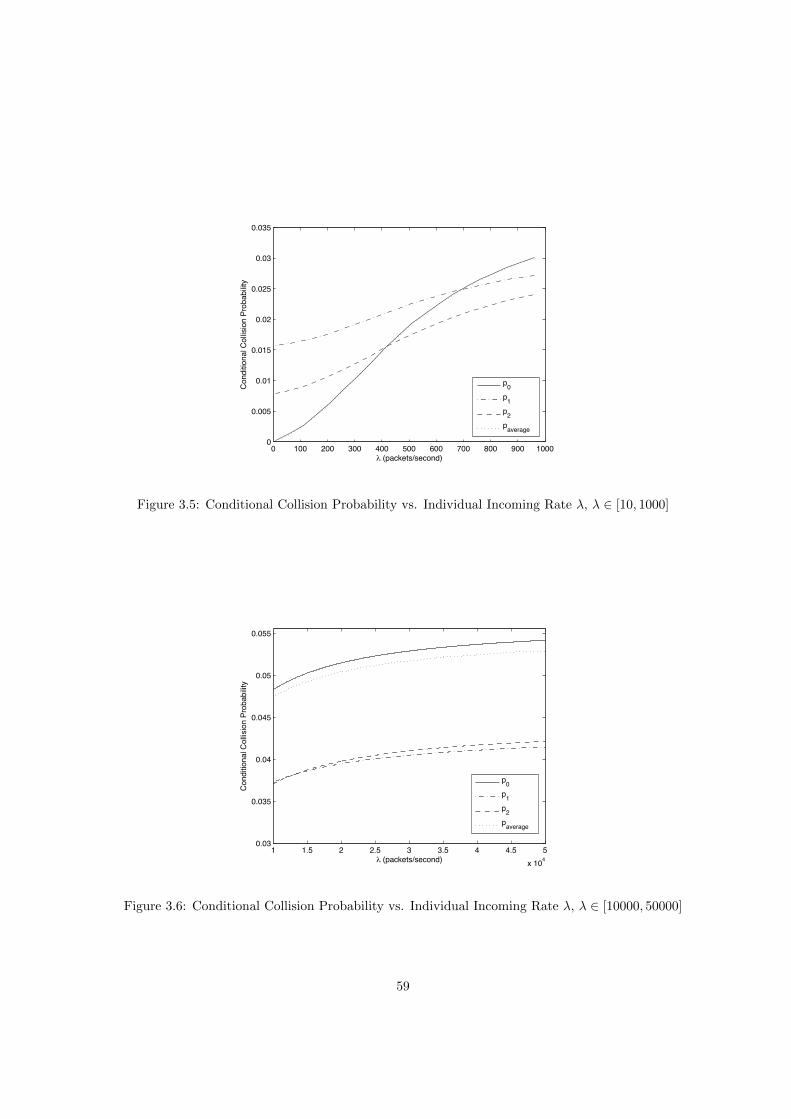
0 100 200 300 400 500 600 700 800 900 10000

0.005

0.01

0.015

0.02

0.025

0.03

0.035

(packets/second)

Con

ditio

nal C

ollis

ion

Prob

abilit

y

p0p1p2paverage


1 1.5 2 2.5 3 3.5 4 4.5 5x 104

0.03

0.035

0.04

0.045

0.05

0.055

(packets/second)

Con

ditio

nal C

ollis

ion

Prob

abilit

y

p0p1p2paverage


59

the limitation on the size of this model that makes its prediction valid only for a specific network, the

general trend observed from its predictions agree with our simulation and experimental observations

for a wide range of other networks (in terms of network size, maximum contention window and back-off

stages). As an explorative research, the smallest model, in terms of numbers of station and back-off

stages, exhibits many interesting features of the data.

60

Chapter 4

On the Queue-decoupling

Hypotheses in IEEE 802.11

Analytical Models

4.1 Introduction

In an unsaturated IEEE 802.11 network, every time after the MAC has transmitted a packet success-

fully or discarded it, it checks the station’s buffer to see if there is another packet awaiting processing.

As mentioned in Section 2.3.2, define Qk := 1 if there is at least one packet awaiting processing

after the kth successful transmission or packet discard and Qk := 0 if the buffer is empty. As it is

technically challenging to fully model the resulting queueing dynamics while still obtaining tractable

equations that can be solved more quickly than a simulation can be run, authors typically employ a

queue-decoupling assumption that can be distilled into the following two hypotheses as described in

Section 2.3.2:

(A3) The sequence {Qk} consists of independent random variables.

(A4) The sequence {Qk} consists of identically distributed random variables that, in particular, do

not depend on the back-off stage.

61

Defining P (Qk = 1) = q, the value of q is typically identified with the steady state probability that an

associated M/G/1/B queueing system has a non-empty buffer after a successful transmission (e.g. [11]

[94]). The M/G/1/B queue is Kendall’s notation [124] for a single-server queue using the first-come

first-served policy where the inter-arrival times are independent and exponentially distributed (M),

the service times are independent and generally distributed (G), and the buffer can hold at most B

packets.

In Section 2.3.2, using detailed statistical analysis of data from simulations and experiments, we

have demonstrated the appropriateness of the first queue-decoupling approximation (A3) and the

inappropriateness of the second queue-decoupling approximation (A4). Despite this flaw, models

based on this queue-decoupling approximation are reported to make accurate network throughput

predictions. In this chapter, we identify where this flawed hypothesis can lead to prediction errors. We

do this by considering the simplest setting where the queue-decoupling hypothesis (A4) can be adopted

or completely avoided so that the impact of the hypothesis can be comparatively investigated. We

show that the models that do and do not incorporate this assumption make near identical throughput

predictions for symmetrically loaded networks, which is a common model validation scenario, but that

their predictions differ when the network is asymmetrically loaded, as is typically the case in practice.

For instance, in a network with 2 stations where the incoming rate (packets per second) of station 1,

λ1, is 10 times as large as that of station 2, λ2, Fig. 4.1 shows the predicted throughput from models

with or without the second queue-decoupling approximation (A4), as well as ns-2 simulation results.

It is clear that this queue-decoupling hypothesis (A4) can cause prediction errors.

The work in this chapter was performed in collaboration with Dr. Ken Duffy (NUIM). Some of

these results have been published in [63]. In Section 4.2, a general analytical model derived from

the mean-field Markov model is introduced. The differences between models with or without the

queue-decoupling assumption (A4) are analytically compared in Section 4.3. Section 4.4 displays the

corresponding simulation results, and conclusions are drawn in Section 4.5.

62

0 500 1000 1500 20000

50

100

150

200

250

300

350

400

450

500

Network Input (Packets/s)

Indi

vidu

al T

hrou

ghpu

t (P

acke

ts/s

)

λ1/λ

2=10

Sim. Class 1Sim. Class 2Var−q Class 1Var−q Class 2Const−q Class 1Const−q Class 2

Figure 4.1: Asymmetric offered load, N=2. ‘Const-q’ and ‘Var-q’ are the models with or without the

queue-decoupling hypothesis (A4), respectively. Theoretical predictions and ns-2 simulations

4.2 A General Analytical Model for Unsaturated Stations with

Small Buffers

The basic structure of the models introduced here is similar to nearly all of those developed from

Bianchi’s paradigm. The models are specifically chosen as they form the simplest situation where an

analytical model can be developed with or without the queue-decoupling hypothesis (A4). By small

buffers, in this chapter we mean the buffers that can hold at most one packet beyond the one being

processed by the MAC, B = 1.

At the heart of IEEE 802.11 DCF algorithm is the Binary Exponential Back-off (BEB) introduced

in Appendix A. Fig. 4.2 shows the general structure of the models we adopt in this chapter. When

a packet arrives at the MAC layer, the back-off stage counter, i, is initiated to 0 and the contention

window Wi is set to be Wmin, the minimum contention window defined in IEEE 802.11 protocol

[120]. Then, an integer back-off counter is randomly and uniformly chosen in {0, 1, · · · ,Wi − 1}.

Time is slotted in this model. In each idle slot, we assume the station has a fixed probability τ of

attempting transmission, which is called the transmission probability. If there exists any other station

also transmitting at the same slot as this station, a collision occurs, and these colliding stations increase

63

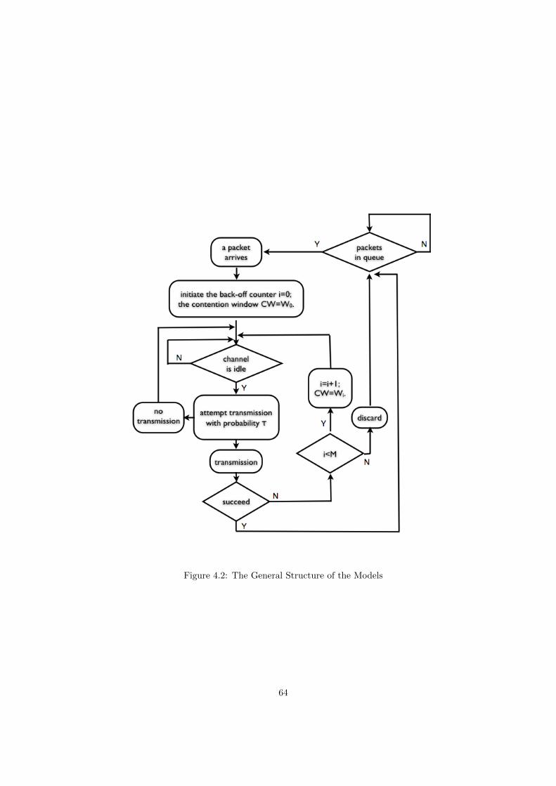
Figure 4.2: The General Structure of the Models

64

their back-off counters, i, by one, set their contention window Wi = 2iWmin, and choose new back-off

counters randomly and uniformly within the new contention window, Wi. To avoid a long waiting

time, the protocol defines an upper limit on the size of the contention window, Wmax = 2mWmin:

Wi = 2mWmin for all i ≥ m.

To avoid a long possession of the MAC service by one packet, the protocol also defines an upper limit

on the number of retries made for a packet. If the back-off stage counter, i, exceeds the retry limit,

M , this packet is discarded. After the packet is successfully transmitted or discarded, the station

checks if any other packets are awaiting in the queue. If not, the station goes into the idle state until

a new packet arrives. With a new packet at the MAC layer, the station resets i = 0, and re-runs the

procedure described above.

Define Ck := 1 if the kth transmission attempt of the station results in a collision, and Ck := 0 if it

results in a successful transmission. We assume the sequence of outcomes of attempted transmissions,

{Ck}, forms a stochastically independent sequence ((A1) in Section 2.3.1). Let the sequence {αk}

record the back-off stage at which the kth transmission attempt is made. We define the conditional

collision probability:

p := P (Ck = 1).

Similarly, we can also define the conditional collision probability pi at the back-off stage i as:

pi := P (Ck = 1|αk = i).

In Section 2.3.1, in an unsaturated network with small buffers, we demonstrate the appropriateness of

the approximation that the sequence {Ck} consists of identically distributed random variables that,

in particular, do not depend on past collision history ((A2) in Section 2.3.1). Thus, we approximate:

pi ≈ p for 0 ≤ i ≤M.

Define Ok := 1 if the station transmits at the kth slot, and Ok := 0 otherwise. We assume the sequence

{Ok} consists of independent and identically distributed (i.i.d.) random variables. We also assume

the transmission sequence {Ok} of every station in the network is independent of every other one,

which means the transmission attempts of every station in the network are independent of each other.

We define the transmission probability, τ , as:

τ := P (Ok = 1).

65

As introduced in Section 4.1, we use the sequence {Qk} to record the status of the queue after the

service of the kth packet. As demonstrated in Chapter 2, the queue-busy sequence {Qk} consists of

almost pairwise independent random variables ((A3) in Section 2.3.2). Let the sequence {βk} record

the back-off stage when the service of the kth packet finishes. Thus, we have:

βk =

Gk∑j=Gk−1

Cj for k > 0,

where Gk = inf{j : Cj = 0, j > Gk−1} and G0 = 0. Since the collision sequence {Ck} is assumed to

be an i.i.d. sequence, it is easy to prove that the sequence {βk} is also an i.i.d. sequence.

Instead of assuming the queue-busy sequence {Qk} consists of i.i.d. random variables ((A4) in Section

2.3.2), we assume the subsequences {Qk|βk = i} are made up by i.i.d. random variables. Thus, we

have the queue busy probability, qi, at the back-off stage i as:

qi := P (Qk = 1|βk = i).

Since in this model we assume the incoming traffic follows a Poisson process, the probability that at

least one packet arrives during a slot, r, can be expressed as a function of incoming rate, λ (packets

per second), and the slot time length, which will be described in Section 4.3.

In this chapter, we use the renewal-reward theorem [46] to derive an expression for the transmission

probability, τ , as a function of the conditional collision probability, p, and the incoming rate, λ, in the

Poisson process.

Renewal-reward theorem: If the sequence {Sk} records the length of the kth renewal epoch,

the sequence {Zk} records the number of rewards obtained in the kth renewal, and Yt is

the total number of rewards obtained in these renewals that are finished before time t,

then we have:

limt→∞

E(Yt)

t=E(Zk)

E(Sk),

where the function E(·) is the expectation function.

Let Sk be the interval time (in slots) between the queue departure time of the kth packet to the queue

departure of the (k + 1)th packet. Sk is the sum of the service time of the kth packet, Ak, and the

66

waiting time for the (k + 1)th packet, Bk+1. Thus, we have:

Sk = Ak +Bk+1.

If there is no packet awaiting in the queue after the service of the kth packet finishes at the back-off

stage i, which happens with the probability (1− qi), the station needs to wait for the (k+ 1)th packet.

As the incoming traffic follows a Poisson process, with the arriving probability during one slot being

r, the average waiting time is 1/r. If there is at least one packet when the station checks the queue,

the waiting time is 0. Thus we have E(Bk) as:

E(Bk) =

1/r if Qk−1 = 0,

0 if Qk−1 = 1.

As we assume, in this model the aggregate attempt process of the other stations is independent of

the back-off process of the tagged one, the incoming traffic follows a Poisson process, and the buffer

size is 1. This model forms a M/G/1/1 queue model. Thus the service times, {Ak} are i.i.d. The

waiting times, {Bk}, depend on the queue-busy probability. The subsequences, {Bk|Qk−1 = 0} and

{Bk|Qk−1 = 1} are i.i.d sequence, respectively. Since the incoming traffic is assumed to be a Poisson

process with incoming rate, λ, we have:

P (Qk = 1) = 1− exp(−λAk−1T ),

where T is the time (in seconds) of an average slot that will be described in detail in Section 4.3.1.

Therefore, the interval time, {Sk}, as the sum of {Ak} and {Bk+1}, is also i.i.d. Since there exists

an upper limit on the service time and the incoming rate, λ, is positive, we have 0 ≤ E(Sk) < ∞.

Therefore, we use Sk as the renewal interval in the renewal-reward theorem.

Define for each n > 0, the random variable:

Jn =

n∑k=1

Sk for n > 0,

which is called the nth jump in the renewal-reward theorem. Then we have the following random

variable:

Xt =

∞∑k=1

1(Jk≤t) = sup{n : Jn ≤ t},

where function 1(Jk≤t) equals 1 when Jk ≤ t and 0 otherwise. This Xt is called the renewal process

in the renewal-reward theorem.

67

Let Zk be the number of transmission attempts made for the kth packet. As βk records the back-off

stage when the service of the kth packet finishes, we have Zk = βk + 1. Since the elements in the

sequence {βk} are i.i.d., it is easy to prove that Zk is also i.i.d. Thus, Zk records the number of

rewards obtained in the kth renewal. Due to its definition, we can have another expression of Zk:

Zk =

∑Jkj=1Oj for k = 1,∑Jkj=Jk−1

Oj for k > 1.

(4.1)

Due to its retry limit, Zk has its upper limit as M + 1. Then, with Eq. (4.1), we call the random

variable:

Yt =

Xt∑k=1

Zk =

Xt∑k=1

Jk∑Jk−1

Oj =

JXt∑j=1

Oj , (4.2)

as the renewal-reward process in the renewal-reward theorem. As described in Eq. (4.2), Yt records the

total number of transmission attempts made in time JXt . Thus, E(Yt)/JXt represents the transmission

probability in one slot during time JXt. According to previous descriptions, we know JXt

< t and the

relationship between them can be written as:

t = JXt+ s,

where

0 ≤ s < sup{Sk : k > 0}.

When t→∞, we have:

limt→∞

JXt

t= limt→∞

t− st

= 1.

Therefore, the following relationship can be obtained:

limt→∞

E(Yt)

t= limt→∞

E(Yt)

JXt

.

The transmission probability τ can be expressed as:

τ = limt→∞

E(Yt)

JXt

= limt→∞

E(Yt)

t. (4.3)

According to the renewal-reward theorem [46], we rewrite Eq. (4.3) as:

τ = limt→∞

E(Yt)

t=E(Zk)

E(Sk),

68

where E(Zk) is the average number of transmission attempts made for the kth packet and E(Sk) is

the average length (in slots) of the kth renewal interval.

According to the BEB algorithm, with the conditional collision probability p, we have:

E(Zk) = 1 + p+ p2 + · · ·+ pM =1− pM+1

1− p. (4.4)

In the renewal interval Sk, using the additional information provided by sequence {βk} that records

the back-off stage counter i at which the service of the kth packet finishes, we have the average renewal

interval time given the service of this packet is finished at the back-off stage j as:

E(Sk|βk = j) =

j∑i=0

Ei + (1− qj)1

r, (4.5)

where Ei is the average time spent at the back-off stage i and 1/r is the average waiting time for the

(k+1)th packet if there is no packet in the queue after the service of the kth packet that is transmitted

at the back-off stage j. The back-off counter is uniformly distributed in {0, 1, · · · ,Wi−1} at the back-

off stage i, and the station can only transmit when the back-off counter is 0 as defined in the protocol

[120]. Thus the back-off waiting times in slots at the back-off stage i are also uniformly distributed in

{0, 1, · · · ,Wi − 1}. Considering it takes one slot time to transmit the packet, the average time spent

at the back-off stage i is:

Ei =

Wi−1∑j=0

1

Wij + 1 =

Wi + 1

2=

2iWmin+1

2 for 0 ≤ i < m,

2mWmin+12 for m ≤ i ≤M.

(4.6)

With Eq. (4.6), we can rewrite Eq. (4.5) as:

E(Sk|βk = j) =

j∑i=0

Ei + (1− qj)1

r=

j∑i=0

Wi + 1

2+ (1− qj)

1

r.

Since the sequence {βk} consists of i.i.d. random variables, due to the BEB algorithm, we have

P (βk = i) = (1− p)pi. Therefore, we can have the expression of E(Sk) as:

E(Sk) =

M∑j=0

E(Sk|βk = j)P (βk = j) =

M∑j=0

(j∑i=0

Wi + 1

2+ (1− qj)

1

r

)(1− p)pj ,

=1

2

(1− pM+1

1− p+Wmin

(1− p− 2mpm+1

(1− p)(1− 2p)− 2mpM+1

1− p

))+

(1− p)r

M−1∑j=0

pj(1− qj) +pM (1− qM )

1− p

,

= η.

(4.7)

69

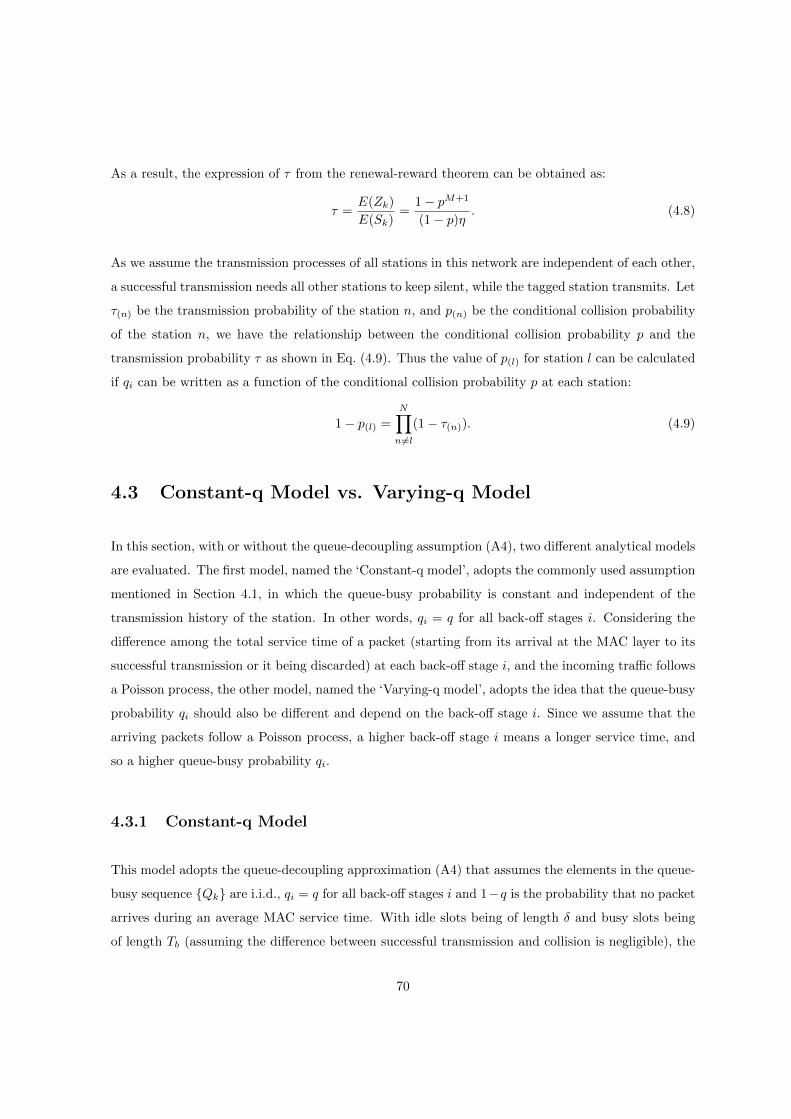
As a result, the expression of τ from the renewal-reward theorem can be obtained as:

τ =E(Zk)

E(Sk)=

1− pM+1

(1− p)η. (4.8)

As we assume the transmission processes of all stations in this network are independent of each other,

a successful transmission needs all other stations to keep silent, while the tagged station transmits. Let

τ(n) be the transmission probability of the station n, and p(n) be the conditional collision probability

of the station n, we have the relationship between the conditional collision probability p and the

transmission probability τ as shown in Eq. (4.9). Thus the value of p(l) for station l can be calculated

if qi can be written as a function of the conditional collision probability p at each station:

1− p(l) =

N∏n 6=l

(1− τ(n)). (4.9)

4.3 Constant-q Model vs. Varying-q Model

In this section, with or without the queue-decoupling assumption (A4), two different analytical models

are evaluated. The first model, named the ‘Constant-q model’, adopts the commonly used assumption

mentioned in Section 4.1, in which the queue-busy probability is constant and independent of the

transmission history of the station. In other words, qi = q for all back-off stages i. Considering the

difference among the total service time of a packet (starting from its arrival at the MAC layer to its

successful transmission or it being discarded) at each back-off stage i, and the incoming traffic follows

a Poisson process, the other model, named the ‘Varying-q model’, adopts the idea that the queue-busy

probability qi should also be different and depend on the back-off stage i. Since we assume that the

arriving packets follow a Poisson process, a higher back-off stage i means a longer service time, and

so a higher queue-busy probability qi.

4.3.1 Constant-q Model

This model adopts the queue-decoupling approximation (A4) that assumes the elements in the queue-

busy sequence {Qk} are i.i.d., qi = q for all back-off stages i and 1−q is the probability that no packet

arrives during an average MAC service time. With idle slots being of length δ and busy slots being

of length Tb (assuming the difference between successful transmission and collision is negligible), the

70

expected time between counter decrements is

T :=

N∏n=1

(1− τ(n))δ +

(1−

N∏n=1

(1− τ(n))

)Tb,

where∏Nn=1(1−τ(n)) is the probability that no station transmits in this slot (the probability of having

an idle slot) and(

1−∏Nn=1(1− τ(n))

)is the probability that any station transmits in this slot (the

probability of having a busy slot).

Thus the average MAC service slots (the number of slots from when the packet starts being processed

by the MAC layer to its successful transmission or it being discarded) is

E(A) = E(E0) + pE(E1) + · · ·+ pmE(Em) + pm+1E(Em+1) + · · ·+ pME(EM );

=W0 + 1

2+ p

W1 + 1

2+ · · ·+ pm

Wm + 1

2+ pm+1Wm+1 + 1

2+ · · ·+ pM

WM + 1

2;

=Wmin + 1

2+ p

2Wmin + 1

2+ · · ·+ pm

2mWmin + 1

2+ pm+1 2mWmin + 1

2+ · · ·+ pM

2mWmin + 1

2;

=Wmin

2

(1− p− 2mpm+1

(1− p)(1− 2p)− 2mpM + 1

1− p

)+

1

2

1− pM+1

1− p.

As the packet arrival process is Poisson, we use the standard approximations 1− r = exp(−λT ), and

1− q = exp(−λE(A)T ) = (1− r)E(A) [94], so that Eq. (4.7) reduces to be

η =1

2

(1− pM+1

1− p+Wmin

(1− p− 2mpm+1

(1− p)(1− 2p)− 2mpM+1

1− p

))+

(1− p)r

(∑M−1

i=0pi(1− q) +

pM

1− p(1− q)

);

=1

2

(1− pM+1

1− p+Wmin

(1− p− 2mpm+1

(1− p)(1− 2p)− 2mpM+1

1− p

))+

(1− p)(1− q)r

(∑M−1

i=0pi +

pM

1− p

);

=1

2

(1− pM+1

1− p+Wmin

(1− p− 2mpm+1

(1− p)(1− 2p)− 2mpM+1

1− p

))+

(1− p)(1− q)r

(1− pM

1− p+

pM

1− p

);

=1

2

(1− pM+1

1− p+Wmin

(1− p− 2mpm+1

(1− p)(1− 2p)− 2mpM+1

1− p

))+

(1− q)r

;

=1

2

(1− pM+1

1− p+Wmin

(1− p− 2mpm+1

(1− p)(1− 2p)− 2mpM+1

1− p

))+

(1− r)E(A)

r.

To solve the Constant-q model, one selects station parameters, including input rates {λi} for i ∈

{1, 2, · · · , N}, and searches for a solution of Eq. (4.9)1.

4.3.2 Varying-q Model

In this ‘Varying-q Model’ that avoids the queue-decoupling approximation (A4), we wish to assume as

little as possible beyond Bianchi’s collision decoupling hypothesis. This leads us to treating slots being

1Empirically, we can always find out a solution of this equation.

71

idle or busy as an i.i.d. process as well as having the queue-busy probability depend on back-off stage.

Therefore, knowing the station l itself has no packet at the MAC layer, the queue-busy probability in

one slot, r, should be an average value of the idle slots and the busy slots:

1− r =∏k 6=l

(1− τk)e−λδ +

1−∏k 6=l

(1− τk)

e−λTb . (4.10)

Knowing the station itself cannot transmit in this slot, on the right side of Eq. (4.10),∏k 6=l(1− τk) is

the conditional probability that this slot is idle, while (1−∏k 6=l(1− τk)) is the conditional probability

that this slot is busy. In Eq. (4.10), the functions e−λδ and e−λTb are the probabilities that at least

one packet arrives during an idle or busy slot, respectively.

Since the service time of a packet can be seen as a sequence of independently selected (idle or busy)

slots, the queue-empty probability, 1 − qi, is as the probability that no packet arrives in any of the

slots in this sequence. For example, the queue-empty probability of back-off stage 0 is:

1− q0 =

(W0−1∑k=0

1

W0(1− r)k

)e−λTb ,

where on the right side of the equation the sum term is the average probability that no packet

arrives during the back-off time and the last term is the probability that no packet arrives during the

transmission time, Tb. Similarly, for back-off stages, i ≥ 1, we have the following recursive expression:

1− qi = (1− qi−1)

(Wi−1∑k=0

1

Wi(1− r)k

)e−λTb for i ≥ 1.

Despite the complexity of the expression for queue-busy probability, qi, it is solely a function of

conditional collision probability, p, assuming one knows all other stations’ parameters. Therefore,

to solve the ‘Varying-q model’, one selects station parameters, including input rates {λi} for i ∈

{1, 2, · · · , N}, and searches for a solution of these equations in addition to the fixed point Eq. (4.9)2.

4.4 Analytical Models Comparison

To compare the accuracy of these two analytical models, ns-2 is used (as described in Appendix D) to

simulate an IEEE 802.11b infrastructure mode network with N stations with small buffers (3 packets

2Empirically, we can always find out a solution of this equation.

72

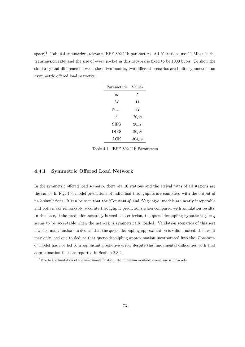
space)3. Tab. 4.4 summarizes relevant IEEE 802.11b parameters. All N stations use 11 Mb/s as the

transmission rate, and the size of every packet in this network is fixed to be 1000 bytes. To show the

similarity and difference between these two models, two different scenarios are built: symmetric and

asymmetric offered load networks.

Parameters Values

m 5

M 11

Wmin 32

δ 20µs

SIFS 20µs

DIFS 50µs

ACK 304µs

Table 4.1: IEEE 802.11b Parameters

4.4.1 Symmetric Offered Load Network

In the symmetric offered load scenario, there are 10 stations and the arrival rates of all stations are

the same. In Fig. 4.3, model predictions of individual throughputs are compared with the output of

ns-2 simulations. It can be seen that the ‘Constant-q’ and ‘Varying-q’ models are nearly inseparable

and both make remarkably accurate throughput predictions when compared with simulation results.

In this case, if the prediction accuracy is used as a criterion, the queue-decoupling hypothesis qi = q

seems to be acceptable when the network is symmetrically loaded. Validation scenarios of this sort

have led many authors to deduce that the queue-decoupling approximation is valid. Indeed, this result

may only lead one to deduce that queue-decoupling approximation incorporated into the ‘Constant-

q’ model has not led to a significant predictive error, despite the fundamental difficulties with that

approximation that are reported in Section 2.3.2.

3Due to the limitation of the ns-2 simulator itself, the minimum available queue size is 3 packets.

73

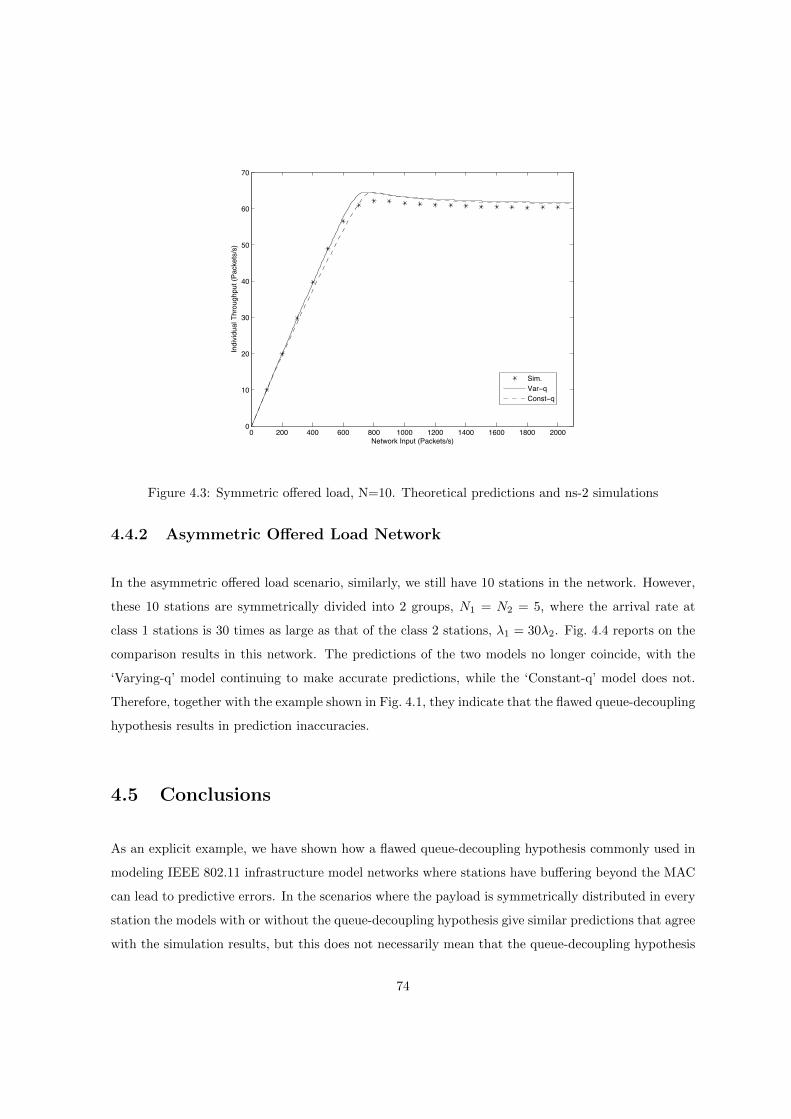
0 200 400 600 800 1000 1200 1400 1600 1800 20000

10

20

30

40

50

60

70


Indi

vidu

al T

hrou

ghpu

t (Pa

cket

s/s)

Sim.Var−qConst−q

Figure 4.3: Symmetric offered load, N=10. Theoretical predictions and ns-2 simulations

4.4.2 Asymmetric Offered Load Network

In the asymmetric offered load scenario, similarly, we still have 10 stations in the network. However,

these 10 stations are symmetrically divided into 2 groups, N1 = N2 = 5, where the arrival rate at

class 1 stations is 30 times as large as that of the class 2 stations, λ1 = 30λ2. Fig. 4.4 reports on the

comparison results in this network. The predictions of the two models no longer coincide, with the

‘Varying-q’ model continuing to make accurate predictions, while the ‘Constant-q’ model does not.

Therefore, together with the example shown in Fig. 4.1, they indicate that the flawed queue-decoupling

hypothesis results in prediction inaccuracies.

4.5 Conclusions

As an explicit example, we have shown how a flawed queue-decoupling hypothesis commonly used in

modeling IEEE 802.11 infrastructure model networks where stations have buffering beyond the MAC

can lead to predictive errors. In the scenarios where the payload is symmetrically distributed in every

station the models with or without the queue-decoupling hypothesis give similar predictions that agree

with the simulation results, but this does not necessarily mean that the queue-decoupling hypothesis

74

0 200 400 600 800 1000 1200 1400 1600 1800 20000

50

100

150

200

250

300

350

400


Indi

vidu

al T

hrou

ghpu

t (Pa

cket

s/s)

!1/!2=30

Sim. Class1Sim. Class2Var−q Class1Var−q Class2Const−q Class1Const−q Class2

Figure 4.4: Asymmetric offered load, N=10. Theoretical predictions and ns-2 simulations

is appropriate. Thus, the only conclusion drawn from these symmetric scenarios is the errors caused

by the queue-decoupling hypothesis are small in this setting. When the network is asymmetrically

loaded, which is common in practice, the error caused by the queue-decoupling hypothesis becomes

significant (the biggest difference between models with and without the queue-decoupling hypothesis

in Fig. 4.4 is about 50 packets/s, 17% of the prediction throughput of the ‘Constant-q’ model). In

order to confidently extrapolate from analytic models that are based on approximations, it is best if

we authenticate their fundamental hypotheses directly rather than the deduction based on them.

75

Chapter 5

Measurements Regarding the

Robustness to Noise of the IEEE

802.11g Rates

5.1 Introduction

In wireless devices, it is well-known that higher transmission rates can lead to lower throughput due to

reduced robustness to channel noise [22]. Consequently the IEEE 802.11 a/b/g WLAN protocol-suite

provides a range of transmission rates determined by distinct physical layer modulation and Forward

Error Correction (FEC) schemes. IEEE 802.11b has four rates (1, 2, 5.5 and 11 Mb/s) operating at

2.4 GHz, IEEE 802.11a has eight rates (6, 9, 12, 18, 24, 36, 48 and 54 Mb/s) operating at 5 GHz,

while IEEE 802.11g has all twelve of the IEEE 802.11a and IEEE 802.11b rates operating at 2.4 GHz.

All of the IEEE 802.11a/b/g rates are summarized in Tab. 5.1, including the FEC rates. In wireless

networks, each station is equipped with a rate control algorithm aiming to select the rate that gives

the highest throughput based on current channel conditions [90], [136].

The IEEE 802.11a/g rates are amenable to theoretical analysis in both Additive White Gaussian

Noise (AWGN), Rayleigh fading, and Rician fading channels [38], [106], [116]. This analysis has

76

shown, surprisingly, that at all signal to noise ratios the IEEE 802.11a 9 Mb/s rate experiences higher

Packet Loss Ratio (PLR1), and hence less throughput, than the 12 Mb/s rate. The observation of this

engineering error has serious implications for rate control algorithms, which should never use the 9

Mb/s rate consequently. In this chapter, we demonstrate the redundancy of the 9 Mb/s by our indoor

and outdoor experimental measurements.

Due to the modulation scheme employed (Complementary Coding Key), the IEEE 802.11b/g rates

of 5.5 and 11 Mb/s are not amenable to theoretical evaluation and must be investigated through

experiments. In this chapter we undertake this task and arrive at a surprising deduction: the 6 Mb/s

IEEE 802.11a/g rate experiences a higher PLR than the 11 Mb/s IEEE 802.11b/g rate in both outdoor

and indoor environments. As the 6 Mb/s rate has a shorter preamble than the 11 Mb/s rate (20µs

instead of 96 or 192 µs [126]), this does not necessarily mean that its throughput is always lower than

that of the 11 Mb/s rate. We show, however, that the advantage conferred by the shorter preamble

at 6 Mb/s is negligible when there is noise on the medium and thus the 6 Mb/s rate is effectively

redundant2.


(NUIM). Some of these results have been published in [67]. Section 5.2 describes the theoretical

analysis of IEEE 802.11a/g rates. A ‘pseudo-theory’ investigation of IEEE 802.11b/g rates in the

presence of noise, based on experimentally fit curves, is presented in Section 5.3. In Section 5.4, for

our experiments to be reproducable, we describe in detail the measurement setup that we used to

assess the available IEEE 802.11g rates, as substantial care is required to avoid complications of the

IEEE 802.11 protocol and its implementation. Section 5.5 displays our experimental results. The

advantage of the short preamble of 6 Mb/s is demonstrated to be negligible for practical purposes in

Section 5.6. This chapter is summarized in Section 5.7.

1We define the PLR to be the fraction of frames that cannot be successfully decoded; on failure to decode, the MAC

layer may re-send the frame, and for PLR we consider this to be a new transmission.2We note the 6Mb/s can be used as the basic rate, rather than a data rate used for payload. In this context, 11

Mb/s is not a direct substitute for 6 Mb/s.

77

Rate (Mb/s) Modulation Scheme FEC Rate In IEEE 802.11a/b/g PHY Layer Technology

1 DBPSK 1/11 b/g DSSS

2 DQPSK 1/11 b/g DSSS

5.5 CCK 4/8 b/g DSSS

6 BPSK 1/2 a/g OFDM

9 BPSK 3/4 a/g OFDM

11 CCK 8/8 b/g DSSS







Table 5.1: IEEE 802.11a/b/g Transmission Rates

5.2 Theory of IEEE 802.11a/g rates

In this chapter, PLR is adopted to quantify the robustness of rates to noise. With a fixed transmission

rate and a fixed SNR3, the PLR is the probability a transmission fails (at the MAC layer) in a

communication between one transmitter and one receiver in the absence of interference from other

stations. The theoretical calculation of PLR depends on channel models [117]. In this section, three

channel models are considered: the Additive White Gaussian Noise (AWGN) channel model, the

Rayleigh fading channel model and the Rician fading channel model.

The AWGN channel model, introduced in Section 5.2.1, is appropriate when there is line of sight

between the transmitter and receiver, but no multi-path, no terrain-blocking and no interference [117].

The Rayleigh fading channel model, introduced in Section 5.2.2, is appropriate in urban environments

when there is no dominant propagation along a line of sight between transmitter and receiver [104].

The model used for Rician fading is similar to that for Rayleigh fading, except that in Rician fading

a strong dominant component is present, which can, for instance, be the line of sight wave [87].

3We reserve SNR for symbol SNR in this chapter.

78

5.2.1 AWGN Channel Model

For the theoretical calculation of PLR as a function of SNR, we begin by using the well-known rela-

tionships between Symbol Error Rate (SER) and SNR that have been derived for different modulation

schemes (BPSK, QPSK and N-QAM) [57] [117]. The SER, Psym, of all modulation schemes used in

IEEE 802.11a/g rates in an AWGN channel can be derived from the SER function in N-ary pulse-

amplitude modulation (N-PAM) [57]:

Psym−N−PAM(SNR) = 2

(1− 1

N

)Q

(√6SNR

N2 − 1

),

where the function Q(·) is the area under the tail of the Gaussian probability density function with

mean zero and unit variance [57]:

Q(x) =1

2erfc

(x√2

).

Since BPSK can be seen as 2-ary PAM, SER of BPSK can be shown as [57]:

Psym-BPSK(SNR) = Psym−2−PAM(SNR). (5.1)

The SER of N-ary quadrature-amplitude modulation (N-QAM) can be also expressed in the form of

PAM as [57]:

Psym−N−QAM(SNR) = 1−(

1− Psym−√N−PAM

(SNR

2

))2

.

Since QPSK can be seen as 4-ary QAM, SER of QPSK can be shown as [57] to be:

Psym-QPSK = Psym−4−QAM. (5.2)

As a Gray code is used to map binary symbols to phasor states for transmission at the PHY layer,

we have the bit error rate at the PHY layer, PB-PHY [69]:

PB-PHY(SNR) =1

kPsym(SNR), (5.3)

where k is the number of bits carried per symbol, k = log2(N).

Since IEEE 802.11a/g rates deploy the convolutional code to provide forward error correction (FEC),

the coding gain should be taken into account in calculating the first error event probability at MAC

layer, PE-MAC. As defined in IEEE 802.11 protocol [120], a Viterbi hard-decision decoder is employed

at the reciver, and PE-MAC can be calculated by the following equation:

PE-MAC =

∞∑d=dfree

ad · Pd(SNR). (5.4)

79

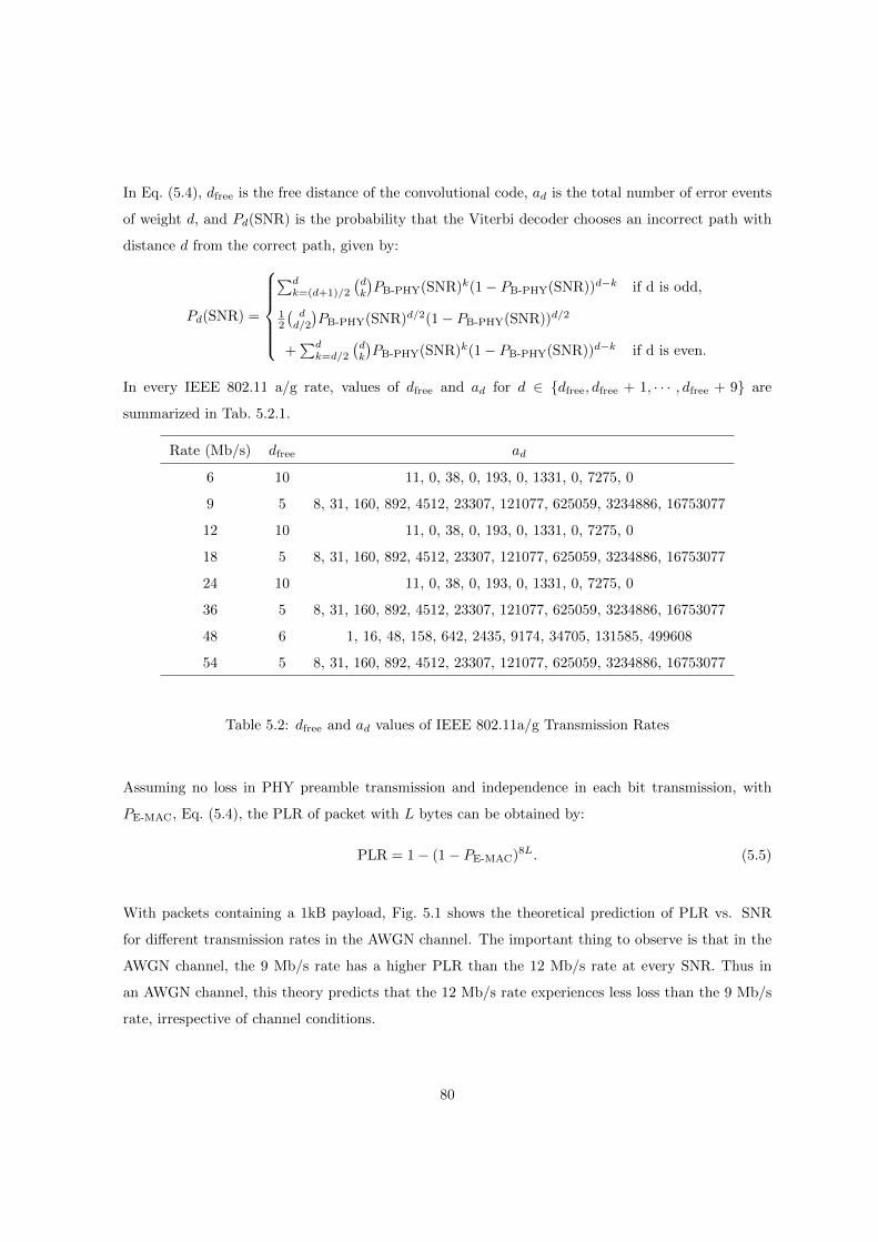
In Eq. (5.4), dfree is the free distance of the convolutional code, ad is the total number of error events

of weight d, and Pd(SNR) is the probability that the Viterbi decoder chooses an incorrect path with

distance d from the correct path, given by:

Pd(SNR) =

∑dk=(d+1)/2

(dk

)PB-PHY(SNR)k(1− PB-PHY(SNR))d−k if d is odd,

12

(dd/2

)PB-PHY(SNR)d/2(1− PB-PHY(SNR))d/2

+∑dk=d/2

(dk

)PB-PHY(SNR)k(1− PB-PHY(SNR))d−k if d is even.

In every IEEE 802.11 a/g rate, values of dfree and ad for d ∈ {dfree, dfree + 1, · · · , dfree + 9} are

summarized in Tab. 5.2.1.

Rate (Mb/s) dfree ad

6 10 11, 0, 38, 0, 193, 0, 1331, 0, 7275, 0

9 5 8, 31, 160, 892, 4512, 23307, 121077, 625059, 3234886, 16753077

12 10 11, 0, 38, 0, 193, 0, 1331, 0, 7275, 0

18 5 8, 31, 160, 892, 4512, 23307, 121077, 625059, 3234886, 16753077

24 10 11, 0, 38, 0, 193, 0, 1331, 0, 7275, 0

36 5 8, 31, 160, 892, 4512, 23307, 121077, 625059, 3234886, 16753077

48 6 1, 16, 48, 158, 642, 2435, 9174, 34705, 131585, 499608

54 5 8, 31, 160, 892, 4512, 23307, 121077, 625059, 3234886, 16753077

Table 5.2: dfree and ad values of IEEE 802.11a/g Transmission Rates

Assuming no loss in PHY preamble transmission and independence in each bit transmission, with

PE-MAC, Eq. (5.4), the PLR of packet with L bytes can be obtained by:

PLR = 1− (1− PE-MAC)8L. (5.5)

With packets containing a 1kB payload, Fig. 5.1 shows the theoretical prediction of PLR vs. SNR

for different transmission rates in the AWGN channel. The important thing to observe is that in the

AWGN channel, the 9 Mb/s rate has a higher PLR than the 12 Mb/s rate at every SNR. Thus in

an AWGN channel, this theory predicts that the 12 Mb/s rate experiences less loss than the 9 Mb/s

rate, irrespective of channel conditions.

80

10 5 0 5 10 15 20 25 3012

10

8

6

4

2

0

SNR (dB)

Pack

et L

oss

Rat

io (L

og10

)

AWGN Channel

6 Mb/s9 Mb/s12 Mb/s18 Mb/s24 Mb/s36 Mb/s48 Mb/s54 Mb/s

Figure 5.1: PLR vs. SNR in an AWGN Channel. Theoretical predictions

5.2.2 Rayleigh Fading Channel

Radio signals suffer reflection, diffraction and scattering when passing through a propagation envi-

ronment with many objects. The received signal at the receiver is a composition of a line of sight

component and multiple reflected, diffracted and scattered signal components. As a consequence,

the amplitude of received signal fluctuates with time. This is known as ‘multipath fading’. Rayleigh

fading is a typical channel model that characterizes a radio channel with multiple paths [104].

The Nakagami-m fading model [117] can be used to describe a wide range of fading models. The

Rayleigh fading channel model is a special case of it with m = 1 (the Nakagami-1 fading model).

Assuming the fading is constant over a packet duration, the BER at the PHY layer of BPSK in a

Nakagami-m fading model with integer m = 1 is given by [117]:

PB-PHY-BPSK =1

2

(1− µBPSK

m−1∑k=0

(2k

k

)(1− µ2

BPSK

4

)k)∣∣∣∣∣m=1

,

=1

2(1− µBPSK) ;

(5.6)

where

µBPSK =

√SNR

m+ SNR

∣∣∣∣∣m=1

=

√SNR

1 + SNR.

81

0 5 10 15 20 25 30 35 4010

9

8

7

6

5

4

3

2

1

0

SNR (dB)

Pack

et L

oss

Rat

io (L

og10

)

Rayleigh Fading Channel


Figure 5.2: PLR vs. SNR in a Rayleigh fading Channel. Theoretical predictions

Similarly, the BER at the PHY layer of N-ary QAM (QPSK equals to 4-ary QAM) in Nakagami-m

fading channel with m = 1 is [117]:

PB-PHY−N−QAM = 4

√N − 1√N

1

log2N

√N/2∑i=1

1

2

1− µN-QAM

m−1∑k=0

(2k

k

)(1− µ2

N−QAM

4

)k∣∣∣∣∣m=1

,

= 4

√N − 1√N

1

log2N

√N/2∑i=1

1

2(1− µN-QAM) ;

(5.7)

where

µN-QAM =

√1.5(2i− 1)2SNR

m(N − 1) + 1.5(2i− 1)2SNR

∣∣∣∣∣m=1

=

√1.5(2i− 1)2SNR

N − 1 + 1.5(2i− 1)2SNR.

As the following Viterbi decoding process in the Rayleigh fading channel model is the same as the one

in the AWGN channel model, we can obtain the PLR function in Rayleigh fading channel by simply

replacing PB-PHY in Eq. (5.4) and (5.5) by the PB-PHY in Rayleigh fading channel given by Eq. (5.6)

and (5.7).

Fig. 5.2 shows the theoretical prediction of PLR vs. SNR for different transmission rates in the

Rayleigh fading channel with 1kB long packets. Predictions in the Rayleigh fading channel model

reveal two redundant rates, 9 Mb/s and 18 Mb/s. As in the AWGN channel, 9 Mb/s suffers more

losses than 12 Mb/s at every given SNR. The rate 18 Mb/s also has higher PLR than 24 Mb/s at

82

every SNR.

5.2.3 Rician Fading Channel

The Rician fading channel is a stochastic model for radio propagation anomaly caused by partial

cancellation of the radio signal by itself. Namely, the signal arrives at the receiver by two different

paths, and at least one of the paths is changing. Rician fading occurs when one of the paths, typically

a line of sight signal, is much stronger than the others. In the Rician fading channel, the K factor

parameter, K, represents the ratio between direct-path (line of sight) power and diffused power.

Therefore, when K = ∞ the Rician fading channel becomes the AWGN channel, and when K = 0

the Rician fading channel is the Rayleigh fading channel [116].

Similarly to the Rayleigh fading channel, we also use Nakagami-m fading model to approximate the

Rician fading channel [117]. The relationship between Nakagami-m and Rician distribution can be

obtained by equating the amount of fading [10]. Thus, we get:

m =1 +K2

1 + 2K.

Therefore, assuming the fading is constant over a packet duration, the BER at the PHY layer of BPSK

is:

PB-PHY-BPSK =1

2

(1− µBPSK

m−1∑k=0

(2k

k

)(1− µ2

BPSK

4

)k)∣∣∣∣∣m= 1+K2

1+2K

,

=1

2

1− µBPSK

1+K2

1+2K−1∑k=0

(2k

k

)(1− µ2

BPSK

4

)k ;

(5.8)

where

µBPSK =

√SNR

m+ SNR

∣∣∣∣∣m= 1+K2

1+2K

=

√SNR(1 + 2K)

1 +K2 + SNR(1 + 2K).

Similarly, the BER at the PHY layer of N-ary QAM (QPSK equals to 4-ary QAM) in the Rician

83

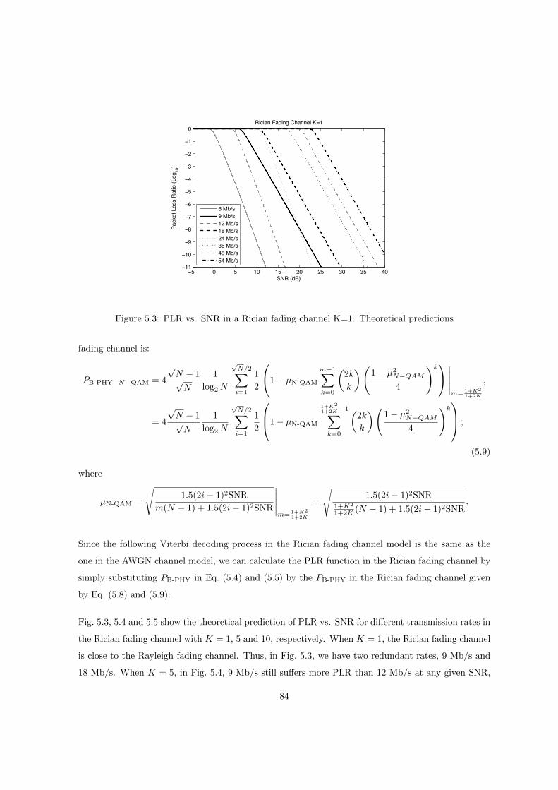
5 0 5 10 15 20 25 30 35 4011

10

9

8

7

6

5

4

3

2

1

0

SNR (dB)

Pack

et L

oss

Rat

io (L

og10

)

Rician Fading Channel K=1


Figure 5.3: PLR vs. SNR in a Rician fading channel K=1. Theoretical predictions

fading channel is:

PB-PHY−N−QAM = 4

√N − 1√N

1

log2N

√N/2∑i=1

1

2

1− µN-QAM

m−1∑k=0

(2k

k

)(1− µ2

N−QAM

4

)k∣∣∣∣∣m= 1+K2

1+2K

,

= 4

√N − 1√N

1

log2N

√N/2∑i=1

1

2

1− µN-QAM

1+K2

1+2K−1∑k=0

(2k

k

)(1− µ2

N−QAM

4

)k ;

(5.9)

where

µN-QAM =

√1.5(2i− 1)2SNR

m(N − 1) + 1.5(2i− 1)2SNR

∣∣∣∣∣m= 1+K2

1+2K

=

√1.5(2i− 1)2SNR

1+K2

1+2K (N − 1) + 1.5(2i− 1)2SNR.

Since the following Viterbi decoding process in the Rician fading channel model is the same as the

one in the AWGN channel model, we can calculate the PLR function in the Rician fading channel by

simply substituting PB-PHY in Eq. (5.4) and (5.5) by the PB-PHY in the Rician fading channel given

by Eq. (5.8) and (5.9).

Fig. 5.3, 5.4 and 5.5 show the theoretical prediction of PLR vs. SNR for different transmission rates in

the Rician fading channel with K = 1, 5 and 10, respectively. When K = 1, the Rician fading channel

is close to the Rayleigh fading channel. Thus, in Fig. 5.3, we have two redundant rates, 9 Mb/s and

18 Mb/s. When K = 5, in Fig. 5.4, 9 Mb/s still suffers more PLR than 12 Mb/s at any given SNR,

84

5 0 5 10 15 20 25 3012

10

8

6

4

2

0

SNR (dB)

Pack

et L

oss

Rat

io (l

og10

)



Figure 5.4: PLR vs. SNR in a Rician fading Channel K=5. Theoretical predictions

10 5 0 5 10 15 20 25 3011

10

9

8

7

6

5

4

3

2

1

0

SNR (dB)

Pack

et L

oss

Rat

io (L

og10

)

Rician Fading Channel, K=10


Figure 5.5: PLR vs. SNR in a Rician fading Channel K=10. Theoretical predictions

85

while the PLR of 18 Mb/s and 24 Mb/s are close to each other, which still suggests 24 Mb/s is better

due to its higher speed. When K = 10, the Rician fading channel has become AWGN-like. Thus,

in Fig. 5.5, we only reveal one redundant rate, 9 Mb/s. Therefore, in the Rician fading channel the

redundancy of 9 Mb/s is observed, irrespective of the value of K, while the case that 18 Mb/s is

redundant depends on the value of K.

Our conclusion is that redundancy of the 9 Mb/s has been demonstrated in the AWGN channel, the

Rayleigh fading channel and the Rician fading channel. In the Rayleigh channel model and Rician

fading channel with K = 1 and 5, the 18 Mb/s rate is also redundant, but not in the AWGN channel

and the Rician fading channel with K = 10. Experiments aiming to verify redundancies of 9 Mb/s

and 18 Mb/s are described in Section 5.5.

5.3 Pseudo-theory of IEEE 802.11b/g rates

Tab. 5.1 also summarizes information on all IEEE 802.11b/g rates. Since 5.5 Mb/s and 11 Mb/s use

CCK, it is not possible to predict their characteristics theoretically [103]. While the IEEE 802.11b/g

5.5 Mb/s and 11 Mb/s rates are not amenable to theoretical investigation, they are subject to pseudo-

theory using experimentally determined relationships. For the consistency of this section, we use

empirical functions quoted from the same source for both 1 Mb/s and 2 Mb/s rates. The following

empirical equations show the relationship between BER at the PHY layer and the bit SNR (Sbit) in

a channel that is assumed to resemble AWGN [72]:

1. 1 Mb/s

PB-PHY1(Sbit) ≤ Q(

√11Sbit); (5.10)

2. 2 Mb/s

PB-PHY2(Sbit) ≤ Q(√

5.5Sbit); (5.11)

3. 5.5 Mb/s

PB-PHY5.5(Sbit) ≤8

15

(14Q(

√8Sbit) +Q(

√16Sbit)

); (5.12)

86

4. 11 Mb/s

PB-PHY11(Sbit) ≤ 24Q(

√4Sbit) + 16Q(

√6Sbit) + 174Q(

√8Sbit)

+ 16Q(√

10Sbit) + 24Q(√

12Sbit) +Q(√

16Sbit).(5.13)

In the above equations, the function Q(·) is as defined in Section 5.2.1. It is common to use the symbol

SNR instead of bit SNR to describe the received signal. The transition function between SNR and

Sbit is [69]:

Sbit = SNRB

R, (5.14)

where B is the bandwidth (22 MHz) and R is bit-rate (R Mb/s).

To calculate the BER at the MAC layer, it is necessary to take the coding gain into account. The 1

Mb/s and 2 Mb/s rates utilize 11-bit Barker Code [97], while the 5.5 Mb/s and 11 Mb/s rates use

the 8-bit CCK [72]. Therefore, the 1 Mb/s and 2 Mb/s rates have a gain of 10.4 dB [97], and the 5.5

Mb/s and 11 Mb/s rates enjoy a gain of 8 dB [72]. With equations ((5.10)) to ((5.14)) and the above

coding gain, the following equations indicate the relationship between the BER at the MAC layer and

the symbol SNR in the AWGN-like channel model:

PB-MAC1(SNR) = PB-PHY1

(SNR

B

R101.04

);


(SNR

B

R101.04

);

PB-MAC5.5(SNR) = PB-PHY5.5

(SNR

B

R100.8

);


(SNR

B

R100.8

).

Having BER at the MAC layer, and assuming all bit errors in the packet occur independently of each

other with probability PB-MAC, the PLR of packets containing L bytes is:

PLR = 1− (1− PB-MAC)8L.

Based on these formulae and standard theory [57], [72], [117] for all IEEE 802.11a/g rates in an AWGN

channel in Section 5.2.1, we obtain Fig. 5.6. This figure, based on pseudo-theory for IEEE 802.11b/g

87

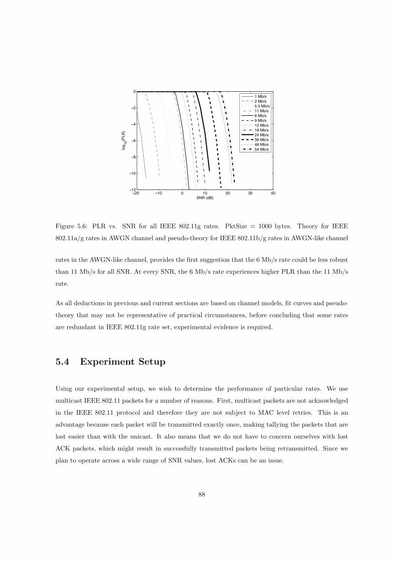
20 10 0 10 20 30 4012

10

8

6

4

2

0

SNR (dB)

log 10

(PLR

)

1 Mb/s2 Mb/s5.5 Mb/s11 Mb/s6 Mb/s9 Mb/s12 Mb/s18 Mb/s24 Mb/s36 Mb/s48 Mb/s54 Mb/s

Figure 5.6: PLR vs. SNR for all IEEE 802.11g rates. PktSize = 1000 bytes. Theory for IEEE

802.11a/g rates in AWGN channel and pseudo-theory for IEEE 802.11b/g rates in AWGN-like channel

rates in the AWGN-like channel, provides the first suggestion that the 6 Mb/s rate could be less robust

than 11 Mb/s for all SNR. At every SNR, the 6 Mb/s rate experiences higher PLR than the 11 Mb/s

rate.

As all deductions in previous and current sections are based on channel models, fit curves and pseudo-

theory that may not be representative of practical circumstances, before concluding that some rates

are redundant in IEEE 802.11g rate set, experimental evidence is required.

5.4 Experiment Setup

Using our experimental setup, we wish to determine the performance of particular rates. We use

multicast IEEE 802.11 packets for a number of reasons. First, multicast packets are not acknowledged

in the IEEE 802.11 protocol and therefore they are not subject to MAC level retries. This is an

advantage because each packet will be transmitted exactly once, making tallying the packets that are

lost easier than with the unicast. It also means that we do not have to concern ourselves with lost

ACK packets, which might result in successfully transmitted packets being retransmitted. Since we

plan to operate across a wide range of SNR values, lost ACKs can be an issue.

88

In our experiments the first 80 bytes of payload in each packet are used to record the experiment

sequence number and transmission rate. The full payload is 1000 bytes and the remaining payload

bits were chosen randomly by a Bernoulli (1/2) process for each packet. We do this in order to ensure

that a wide variety of symbols are used at the physical layer. While IEEE 802.11 does XOR with a

scrambling sequence before transmission, there are only 127 possible scrambling sequences. By using a

random payload we mitigated the risk of repeatedly testing the transmission of the same bit sequences.

Packet transmissions are spaced so that there is sufficient time to send each packet before the next is

queued, thus avoiding losses due to buffer overflows.

Two laptops equipped with Atheros IEEE 802.11b/g cards are used, one employed as a transmitter

and one as a receiver. Both are equipped with a modified version of the MadWifi driver [3]. One

laptop is configured to act as an access point (using host AP mode) while the other is configured as

a station. Our multicast frames are sent from the AP to the station. Note that sending in the other

direction would result in the frame being unicast to the AP first, and then multicast from the AP.

Ideally, we would like each packet to be transmitted in the same manner, so we fix transmission power

at the sender and fix which antenna was used for transmission. The driver is modified to enable the

selection of a fixed transmission rate for multicast data packets. At the receiver, a certain amount

of adaptation cannot be avoided (for example, hardware signal equalization), however we do modify

the driver to disable disassociation due to missed beacons. This prevents the driver from scanning

for new access points when the signal level to the current access point is so low that beacon frames

cannot be successfully decoded. We also disable Atheros’s Ambient Noise Immunity (ANI) feature,

which has been reported to cause unwanted side effects [125]. They observe that ANI can disable the

reception of packets at 6 Mb/s with low signal strength, while not having an impact on the reception

of packets transmitted at 11 Mb/s. This can result in large differences in PLR due to ANI.

While validating our setup, we send sequences of packets and record if each packet was successfully

received or not. Thus, a loss sequence {Lk} is built up with Lk = 0 when the kth packet transmitted

successfully and Lk = 1 otherwise.

We initially conduct tests in a playing field some distance from any buildings, roads and other sources

of interference, as confirmed using a spectrum analyzer. We check the resulting loss sequences for

evidence of correlation by examining the auto-covariance of the loss sequence. In a simply memoryless

channel without interfering devices, packet losses are expected to be independent, so we regarded

non-zero covariance as evidence of pair-wise interference, higher-layer adaptation, etc. that should be

89

0 20 40 60 80 100 120 1400

0.1

0.2

0.3

0.4

0.5

0.6

0.7

0.8

0.9

1

Time Scale (t)

Loss

Seq

uenc

e

Figure 5.7: Smoothed loss sequence with smoothing constant α = 0.2, separation 20m and rate 54

Mb/s. For the first section, people are walking between laptops. For the middle section, people are

hidden. For the last section people are standing behind laptops.

eliminated from clean-environment performance.

We also inspect the loss sequence smoothed with an exponential sliding average (for the arrival of

packet k, Yk+1 = αLk+1 + (1 − α)Yk and α = 0.2, which is plotted against the packet transmission

time). For example, Fig. 5.7 shows the smoothed loss rate in the following case. The two laptops

are set up in a playing field 20 meters apart. During the first part of the experiment (approximately

t from 0 to 60s), the two operators walk between the two laptops. In the second part of the trace

(approximately t from 60 to 100s), the operators stay 10 meters away from the experiment site and

hide behind trees, so there is no direct line-of-sight from them to the laptops. In the final part, the

operators stand still on a point approximately 1 meter behind the laptops (approximately t from 100

to 140s). The behavior of the loss sequence is clearly different for each part of the experiment.

Fig. 5.8 shows the auto-covariances of the loss sequences observed during each part of this mea-

surement. We note that the first and last sections of the experiment, where people are near the

experimental devices, represents a significant source of correlation remaining as high as 0.1 even after

tens of seconds. On the contrary, when people are removed from the picture the auto-covariance

quickly decays to less than 0.1 and stays there. This confirms previous results that the human motion

heavily influences measurement outcomes [15], and so for our clean-environment results we aim to

90

minimize the impact of moving people. Naturally, the impact of moving people is often an important

part of the WiFi environment, and our office based results include people. However, it is useful to

study the behavior of our equipment in a relatively static environment, to build confidence that we are

really testing the low layer channel performance, and not simply observing a changing environment

or a higher layer adaptation mechanism.

0 10 20 30 40 50−0.2

0

0.2

0.4

0.6

0.8

1

1.2In the way

Time Lag (t)

Auto

Cov

(a) In the way

0 10 20 30 40 50 60−0.2

0

0.2

0.4

0.6

0.8

1

1.2Far Away

Time Lag (t)

Auto

Cov

(b) Far away

0 5 10 15 20 25 30 35−0.2

0

0.2

0.4

0.6

0.8

1

1.2On the Point

Time Lag (t)

Auto

Cov

(c) On the point

Figure 5.8: Auto-covariance for sections of the loss sequence against lag in seconds. For the first

section, people are walking between laptops. For the middle section, people are hidden. For the last

section people are standing behind laptops.

Our measurements are repeated with the laptops separated by increasing distances to vary the path

SNR in a stable environment. The ground is not level and if the laptops are close to the ground then

line-of-sight could be obscured. To avoid this, we place each laptop on a 75 centimeters tall plastic

pedestal, to ensure that the direct path was not obscured.

91

5.5 Experiment Results

Using the experimental apparatus described in the previous section, we performed extensive measure-

ments in two distinct environments, outdoor experiments on a sports field and indoor experiments in

an office environment. We expect the outdoor environment to be representative of a relatively simple

channel, with line-of-sight being the primary signal path. We expect the indoor environment to be

more complex, and so conduct tests at night when the environment is relatively static and during

the day when people, doors and other objects move frequently. As described in the previous section,

significant efforts are made to check that we are testing the performance of the physical layer. Each

point on a graph in this section represents a measurement outcome from an experiment with 20,000

packets. The error bars based on a Central Limit Theorem approximation for the mean PLR are,

consequently, too small to be shown.

5.5.1 Outdoor Experiments

Fig. 5.9 shows PLR vs. Transmission Rate for the outdoor experiments at a separation of 160 meters.

There are two significant deductions from this graph. First, the 6 Mb/s IEEE 802.11a/g rate expe-

riences more packet loss than the 11 Mb/s IEEE 802.11b/g rate (roughly 25% against 20%). Thus,

while one expects that by design the lower rates will be more robust, this is not the case. Second, the

9 Mb/s IEEE 802.11a/g rate gets no throughput while the 12 Mb/s IEEE 802.11a/g rate experiences

packet loss of approximately 50%.

Since the outdoor environment, where line-of-sight is the primary signal path, can be assumed to

be an AWGN channel, Fig. 5.6 can be considered as predictions on our experimental measurement

results. It is obvious that our experiment observations support our predictions obtained from theory

of IEEE 802.11a/g rates and pseudo-theory of IEEE 802.11b/g rates.

Unlike the non-monotonic pair (9 Mb/s and 12 Mb/s), which has a strong theoretical support, we

want to provide more experimental evidence to verify the non-monotonic pair (6 Mb/s and 11 Mb/s).

As shown using pseudo-theory in Fig. 5.6, 6 Mb/s suffers a bigger PLR than 11 Mb/s at any given

SNR. To test this prediction, a sequence of outdoor experiments were performed to measure PLR

exclusively for the 6 Mb/s and 11 Mb/s rates. Fig. 5.10 shows PLR for 6 Mb/s and 11 Mb/s as the

distance between the sender and receiver is varied. It is clear that SNR is a monotonically decreasing

92

0 10 20 30 40 50

0

0.2

0.4

0.6

0.8

1

Transmission Rate (Mb/s)

Pac

ket L

oss

Rat

e

802.11a/g802.11b/g

Figure 5.9: Measured PLR vs. Transmission Rates in day-time outdoor environment at 160m separa-

tion. Experiment

function of distance in stable environments. These data were obtained on a different day from those

in Fig. 5.9, so that absolute loss rates are different, but the trend is the same. Apart from at distances

where neither rate experiences any packet losses, the clear conclusion is that 6 Mb/s loses more packets

than 11 Mb/s at all distances.

To ensure this conclusion is not a specific feature of the hardware we used, the Atheros IEEE 802.11b/g

card, we re-run our outdoor experiments with an Intel 2200b/g card at the receiver. Fig. 5.11 shows

the PLR vs. all IEEE 802.11g rates at two different scenarios. In the ‘damp’ scenario, the humidity

in the air is high and the two laptops are 65m apart, while in the ‘dry’ scenario, the humidity in the

air is low and the two laptops are 185m apart. It is clear that there exist the non-monotonic pairs (6

Mb/s with 11 Mb/s and 9 Mb/s with 12 Mb/s) in Fig. 5.11. We also measured PLR for 6 Mb/s and

11 Mb/s as the distance between the two laptops varied in a stable environment with the Intel card

at the receiver. Fig. 5.12 shows the fact that 6 Mb/s suffers a bigger PLR than 11 Mb/s at different

distances. Therefore, we have some evidence that the results in this chapter hold in some generality.

93

60 70 80 90 100 110 120 130 140 150 1600

0.1

0.2

0.3

0.4

0.5

0.6

0.7

0.8

0.9

1

Distance (m)

Pack

et L

oss

Rat

e

6 Mb/s Atheros Rx11 Mb/s Atheros Rx6 Mb/s Intel Rx11 Mb/s Intel Rx

Figure 5.10: Measured PLR vs. distance in day-time outdoor environment. Experiment

0 5 10 15 20 25 30 35 40 45 50 55

0

0.2

0.4

0.6

0.8

1

Rate (Mb/s)

Pack

et L

oss

Rat

e

Intel Rx DampIntel Rx Dry

Figure 5.11: Measured PLR vs. Transmission Rates in day-time outdoor environment with Intel

card at the receiver. The distance in the ‘damp’ scenario is 65m and in the ‘dry’ scenario is 185m.

Experiment

94

60 70 80 90 100 110 120

0

0.2

0.4

0.6

0.8

1

Distance (m)

Pack

et L

oss

Rat

e

6 Mb/s Intel Rx.11 Mb/s Intel Rx.

Figure 5.12: Measured PLR vs. distance in day-time outdoor environment with Intel card at the

receiver. Experiment

5.5.2 Indoor Experiments

The indoor night time experiments were carried out at midnight to limit the impact of human motion,

which can cause variation in channel conditions as described in Section 5.4. Fig. 5.13 reports PLR

vs. Transmission Rate for these experiments. For these results, the transmitter and receiver laptops

were placed in separate offices approximately 10 meters apart, with several partition walls between

them. In the plot it can be seen that the 9 Mb/s IEEE 802.11a/g rate suffers a similar PLR to

the 12 Mb/s IEEE 802.11a/g rate. The 11 Mb/s IEEE 802.11b/g rate experiences no loss at this

distance, but the 6 Mb/s IEEE 802.11a/g rate experiences approximately 20% loss. Note that in

these indoor experiments, where one might expect the Rayleigh fading model to be appropriate, they

do not confirm the other non-monotonic prediction (18 Mb/s and 24 Mb/s) given in Section 5.2.2.

A second collection of indoor experiments with the same set-up was performed at mid-day during a

working week to investigate the impact of channel conditions driven by human motion as well as the

switching on and off of computers with wireless cards. For two distinct runs, Fig. 5.14 reports typical

measurements of PLR vs. Transmission Rate. This plot illustrates that although the absolute level of

loss changes based on the environmental conditions, the undesirable PLR ordering seen in the mid-day

measurements remains present. That means, in mid-day time experiment results, 11 Mb/s and 12

95

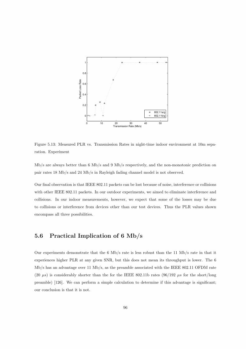
0 10 20 30 40 50

0

0.2

0.4

0.6

0.8

1


Pac

ket L

oss

Rat

e

802.11a/g802.11b/g

Figure 5.13: Measured PLR vs. Transmission Rates in night-time indoor environment at 10m sepa-

ration. Experiment

Mb/s are always better than 6 Mb/s and 9 Mb/s respectively, and the non-monotonic prediction on

pair rates 18 Mb/s and 24 Mb/s in Rayleigh fading channel model is not observed.

Our final observation is that IEEE 802.11 packets can be lost because of noise, interference or collisions

with other IEEE 802.11 packets. In our outdoor experiments, we aimed to eliminate interference and

collisions. In our indoor measurements, however, we expect that some of the losses may be due

to collisions or interference from devices other than our test devices. Thus the PLR values shown

encompass all three possibilities.

5.6 Practical Implication of 6 Mb/s

Our experiments demonstrate that the 6 Mb/s rate is less robust than the 11 Mb/s rate in that it

experiences higher PLR at any given SNR, but this does not mean its throughput is lower. The 6

Mb/s has an advantage over 11 Mb/s, as the preamble associated with the IEEE 802.11 OFDM rate

(20 µs) is considerably shorter than the for the IEEE 802.11b rates (96/192 µs for the short/long

preamble) [126]. We can perform a simple calculation to determine if this advantage is significant;

our conclusion is that it is not.

96

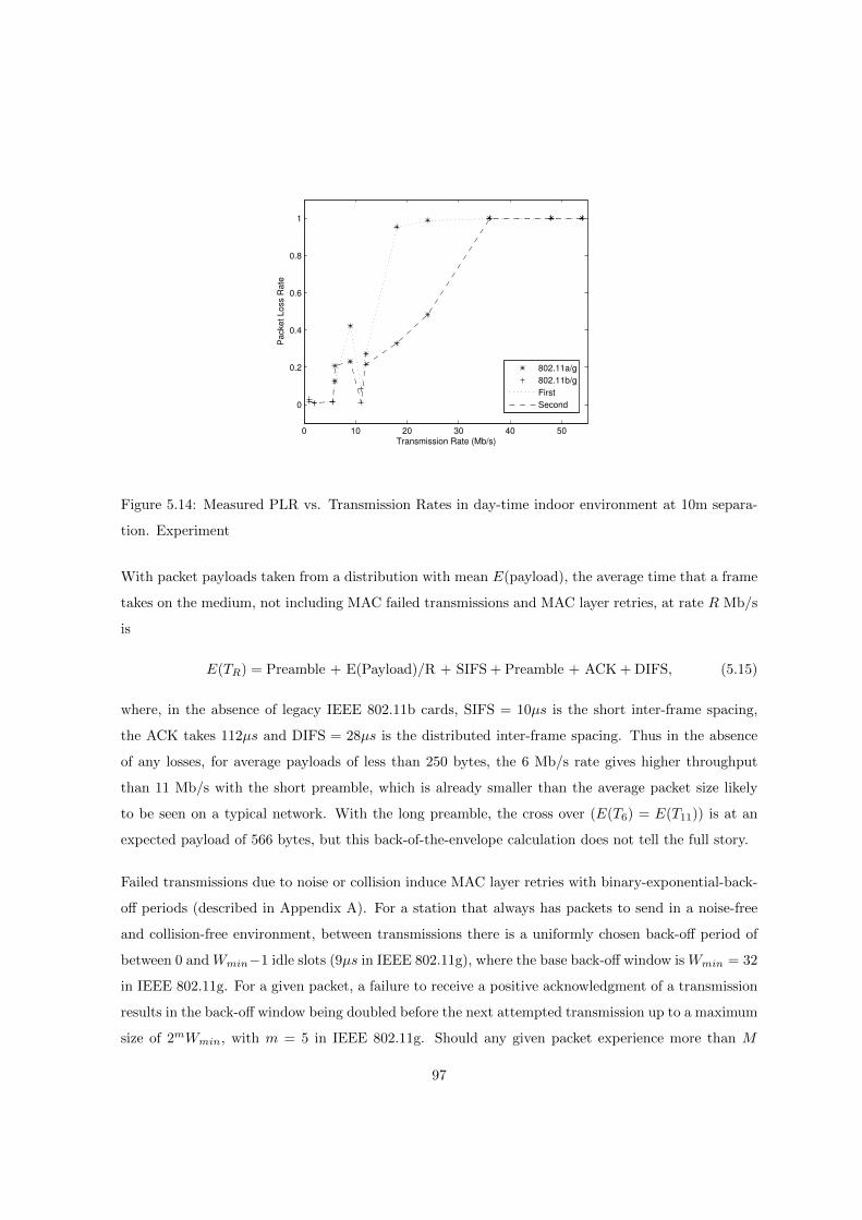
0 10 20 30 40 50

0

0.2

0.4

0.6

0.8

1


Pac

ket L

oss

Rat

e

802.11a/g802.11b/gFirstSecond

Figure 5.14: Measured PLR vs. Transmission Rates in day-time indoor environment at 10m separa-

tion. Experiment

With packet payloads taken from a distribution with mean E(payload), the average time that a frame

takes on the medium, not including MAC failed transmissions and MAC layer retries, at rate R Mb/s

is

E(TR) = Preamble + E(Payload)/R + SIFS + Preamble + ACK + DIFS, (5.15)

where, in the absence of legacy IEEE 802.11b cards, SIFS = 10µs is the short inter-frame spacing,

the ACK takes 112µs and DIFS = 28µs is the distributed inter-frame spacing. Thus in the absence

of any losses, for average payloads of less than 250 bytes, the 6 Mb/s rate gives higher throughput

than 11 Mb/s with the short preamble, which is already smaller than the average packet size likely

to be seen on a typical network. With the long preamble, the cross over (E(T6) = E(T11)) is at an

expected payload of 566 bytes, but this back-of-the-envelope calculation does not tell the full story.

Failed transmissions due to noise or collision induce MAC layer retries with binary-exponential-back-

off periods (described in Appendix A). For a station that always has packets to send in a noise-free

and collision-free environment, between transmissions there is a uniformly chosen back-off period of

between 0 and Wmin−1 idle slots (9µs in IEEE 802.11g), where the base back-off window is Wmin = 32

in IEEE 802.11g. For a given packet, a failure to receive a positive acknowledgment of a transmission

results in the back-off window being doubled before the next attempted transmission up to a maximum

size of 2mWmin, with m = 5 in IEEE 802.11g. Should any given packet experience more than M

97

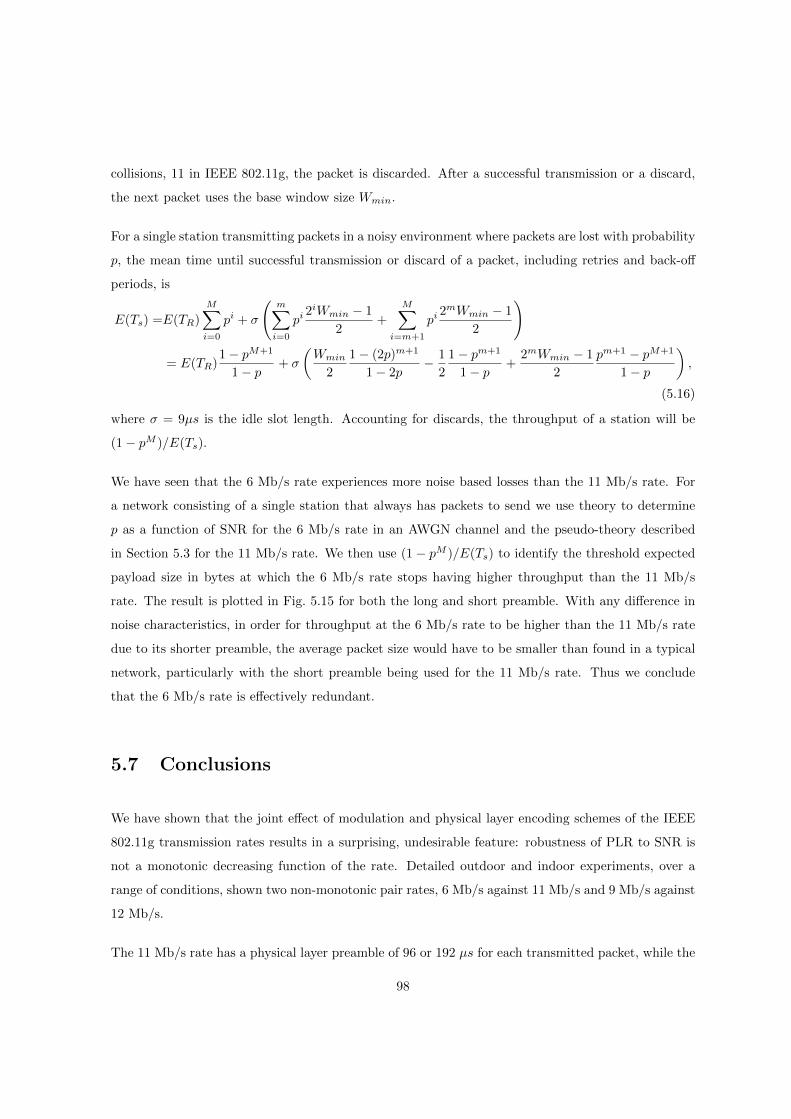
collisions, 11 in IEEE 802.11g, the packet is discarded. After a successful transmission or a discard,

the next packet uses the base window size Wmin.

For a single station transmitting packets in a noisy environment where packets are lost with probability

p, the mean time until successful transmission or discard of a packet, including retries and back-off

periods, is

E(Ts) =E(TR)

M∑i=0

pi + σ

(m∑i=0

pi2iWmin − 1

2+

M∑i=m+1

pi2mWmin − 1

2

)

= E(TR)1− pM+1

1− p+ σ

(Wmin

2

1− (2p)m+1

1− 2p− 1

2

1− pm+1

1− p+

2mWmin − 1

2

pm+1 − pM+1

1− p

),

(5.16)

where σ = 9µs is the idle slot length. Accounting for discards, the throughput of a station will be

(1− pM )/E(Ts).

We have seen that the 6 Mb/s rate experiences more noise based losses than the 11 Mb/s rate. For

a network consisting of a single station that always has packets to send we use theory to determine

p as a function of SNR for the 6 Mb/s rate in an AWGN channel and the pseudo-theory described

in Section 5.3 for the 11 Mb/s rate. We then use (1− pM )/E(Ts) to identify the threshold expected

payload size in bytes at which the 6 Mb/s rate stops having higher throughput than the 11 Mb/s

rate. The result is plotted in Fig. 5.15 for both the long and short preamble. With any difference in

noise characteristics, in order for throughput at the 6 Mb/s rate to be higher than the 11 Mb/s rate

due to its shorter preamble, the average packet size would have to be smaller than found in a typical

network, particularly with the short preamble being used for the 11 Mb/s rate. Thus we conclude

that the 6 Mb/s rate is effectively redundant.

5.7 Conclusions

We have shown that the joint effect of modulation and physical layer encoding schemes of the IEEE

802.11g transmission rates results in a surprising, undesirable feature: robustness of PLR to SNR is

not a monotonic decreasing function of the rate. Detailed outdoor and indoor experiments, over a

range of conditions, shown two non-monotonic pair rates, 6 Mb/s against 11 Mb/s and 9 Mb/s against

12 Mb/s.

The 11 Mb/s rate has a physical layer preamble of 96 or 192 µs for each transmitted packet, while the

98

7 6 5 4 3 2 1 0 10

100

200

300

400

500

600

SNR (dB)

Expe

cted

Pac

ket S

ize

(byt

e)

Long PreambleShort Preamble

Figure 5.15: Single station. Largest expected payload at which the 6 Mb/s rate at given SNR obtains

higher throughput than the 11 Mb/s 6 Mb/s theory and 11 Mb/s pseudo-theory

6 Mb/s rate has a preamble of 20 µs. Thus, despite the higher loss rate, this does not necessarily mean

that the 6 Mb/s rate achieves less throughput. However, by considering the number of retries and

the amount of time a station spends in back-off, we can quantify the conditions under which 6 Mb/s

will offer better throughput. For practically realistic mean payload sizes the rate with the lowest PLR

will, indeed, offer the highest throughput and lowest transmission delays. Thus, while the 6 Mb/s

IEEE 802.11g rate is not necessarily redundant in all stations, it is in most practical ones. Thus both

the 6 and 9 Mb/s IEEE 802.11g rates are effectively redundant and should not be considered by the

rate control algorithm with IEEE 802.11g rates.

99

Chapter 6

H-RCA: IEEE 802.11

Collision-aware Rate Control

6.1 Introduction

IEEE 802.11 is the world’s most commonly deployed WLAN technology. It supports several physical

layer transmission rates, with IEEE 802.11b having four (1, 2, 5.5 and 11 Mb/s), IEEE 802.11a having

eight (6, 9, 12, 18, 24, 36, 48 and 54 Mb/s), while IEEE 802.11g has all twelve of the IEEE 802.11b

and 802.11a rates, and IEEE 802.11n has eight when using two streams at 20 Mhz and a guard

interval of 800ns (13, 26, 39, 52, 78, 104, 117, 130 Mb/s). A range of rates are available as their

modulation and coding schemes give them distinct robustness characteristics to noise on the medium.

To maximize network performance, each station needs to select an appropriate rate for its current

channel conditions. Rate Control (RC) algorithms that choose modulation and coding scheme pairs

are designed for this purpose.

In this chapter we propose a principled design for a RC algorithm, H-RCA, that overcomes the

shortcomings of existing algorithms. This H-RCA is applicable to all IEEE 802.11 rate-sets and is

implementable on commodity hardware. H-RCA’s objective is to minimize the average time each

packet spends on the medium, including MAC layer retries, in a fully decentralized fashion with no

message passing. It employs a development of a cutting-edge censored data technique based on the

100

IEEE 802.11e TXOP feature to distinguish transmission failures caused by collisions from those caused

by noise [56]. H-RCA makes transmission rate choices based on the Packet Loss Rate (PLR) due to

noise alone1, with Bayesian analysis used to determine rate-decrease decisions and an opportunity-cost

metric used to determine the frequency at which rate-increase decisions are made. H-RCA does not

alter the IEEE 802.11 MAC and can be implemented on existing network cards that possess IEEE

802.11e functionality. We give a concrete guide to the approach through detailed consideration of the

IEEE 802.11a rate-set, including performance evaluation in simulation as well as initial results from

an experimental implementation.


(NUIM). Some of these results are included in [65]. The rest of this chapter is organized as follows.

In Section 6.2 we describe related work. The H-RCA paradigm is defined in Section 6.3 and the

reasoning behind its settings explained. As it is not feasible to create an experimental setup with

controllable losses due to noise, Section 6.4 presents ns-2 simulation results illustrating H-RCA’s

performance for an IEEE 802.11a WLAN. These simulations reveal the approach’s merits in terms

of throughput consistency in a fixed environment, adaptivity to changing channel conditions and

robustness to collision-based transmission failures. As experimental systems can expose difficulties

not captured by theory or simulations, in Section 6.5 we report on an experimental implementation of

H-RCA for the IEEE 802.11a rate-set where it shows significant throughput gains over RC algorithms

that are available with current hardware. The chapter concludes with a discussion in Section 6.6.

6.2 Related Work

The IEEE 802.11 standard does not specify details of the RC algorithm to be used, so that IEEE

802.11 card vendors and researchers have proposed and implemented a variety of algorithms. There

are two distinct strategies for RC algorithms. The first is the explorative type. In this approach

the entire rate space is explored periodically to empirically identify the optimal rate. Examples of

algorithms of this type include SampleRate [22], RBAR [62], OAR [112], WOOF [7] and CHARM

[74]. The second strategy is the incremental type where algorithms record statistics regarding their

current rate and its neighboring rates, and make incremental changes. Example RC algorithms of

this type include ARF [75], AARF [83], CARA [78], RRAA [136], SGRA [143], COLLIE [110] and

1We reserve PLR for failures due to noise, not collision.

101

SoftRate [129]. A number of these, including SampleRate, Minstrel [1], Onoe [4] and AMRR [83], are

implemented, for example, on the Atheros chipset.

The choice of rate should be based on current channel conditions, so that a good estimate of channel

quality is key to all RC algorithms. There are two dominant paradigms to measure channel condi-

tions: determine SNR directly from physical layer estimates; or estimate channel conditions indirectly

through packet loss information.

6.2.1 Physical Layer Based Estimates

The ideal information on which to base the choice of the transmission rate is SNR at the receiver.

RBAR [62] uses an RTS/CTS exchange immediately prior to packet transmission to estimate SNR

at the receiver and picks its rate accordingly. OAR [112] builds on RBAR and opportunistically

transmits back-to-back frames using a fragmentation scheme when channel quality is good. CHARM

[74] leverages reciprocity of the wireless channel to estimate average SNR at the receiver using packets

overheard from the receiver to avoid the RTS/CTS overhead. It is not trivial, however, for the

transmitter to accurately estimate the SNR at the receiver because signal strength exhibits significant

variations on a per-packet basis [143].

6.2.2 Packet-Loss Based Estimates

Using packet loss information to infer channel conditions is the second option. Automatic Rate

Fallback (ARF) is a scheme that uses patterns of packet losses as a trigger to change the transmission

rate [75]. Adaptive ARF (AARF) continuously changes the threshold that decides when to try a higher

rate to better reflect current channel conditions [83]. Adaptive Multi Rate Retry (AMRR) is AARF’s

practical realization. Its key idea is to use binary-exponential-backoff to control the probing period to

sample other rates. The algorithm initially switches to a higher data rate when ten consecutive packets

have been transmitted without any failure and moves to a lower rate if two consecutive packets are not

acknowledged. If packet failure occurs when a higher data rate is sampled, the interval for the next

higher data rate sampling is exponentially increased. For these approaches to function correctly in a

network with more than one active transmitter, the algorithm would need a mechanism to distinguish

between transmission failures caused by collision and those caused by noise on the channel.

102

Some algorithms use the RTS/CTS scheme to identify failed transmissions due to collisions. If the

first attempted transmission of a packet fails, CARA [78] uses RTS/CTS to test whether failure is

caused by collision or noise. Since RTS/CTS costs substantial time on the medium, RRAA [136]

reduces the frequency of using RTS/CTS. RRAA uses frame loss information gathered over tens of

frames to adapt the rate and compares frame loss statistics both with and without RTS/CTS in order

to decide if a loss is caused by collision or noise. It adaptively enables RTS/CTS more frequently as

its estimate of the rate of failures due to collisions increases.

To avoid using RTS/CTS, WOOF [7] uses Channel Busy Time (CBT) as an indicator of network load.

Higher CBT means heavier traffic in the network, so that a transmission failure is more likely to be

caused by collision rather than noise. Running at the sender, COLLIE [110] analyzes the patterns

of bit errors in the received packet in order to infer whether an error was due to a collision or the

channel noise. Its rate adaptation protocol then solely depends upon channel noise failures. To detect

bit errors, however, the COLLIE receiver must echo the entire received frame to the sender, incurring

significant overhead. Running at the receiver, SoftRate [129] uses hints exported by the physical layer

to compute the average Bit Error Rate (BER) for each received frame. To exclude failures due to

collisions, it uses the ansatz that a sudden spike in bit errors is likely to have been caused by collision.

The receiver sends its BER estimate to the sender where it picks the best rate for the next frame. In

order to observe the impact of collisions more clearly, it also adds a ‘post-amble’ to every frame to

enable the receiver to detect with high probability the portion of the sender’s frame that lasts after

the interference has ended. Thus SoftRate uses more time per frame on the medium and to implement

it would require changes to hardware.

To avoid hardware modifications, in [35] the authors use the number of idle slots between two con-

secutive busy periods to estimate the number of active stations in the network. Having obtained an

estimate of number of the active stations, using a Bianchi-like model [36], the collision probability

conditioned on transmission can be estimated. Armed with this estimate one can estimate the packet

loss probability due to noise. The information on the number of idle slots is not available, however,

in general commodity cards. Therefore, in [37] the authors overcome this difficulty by using retry in-

formation in IEEE 802.11 MAC headers as an indicator of the channel condition, as each station can

monitor the medium and get access to the MAC header of every packet transmitted in the medium.

If a large number of retransmitted packets are observed, it is inferred that the network is handling a

high traffic load.

103

SampleRate [22] adopts a different strategy. It focuses on minimizing the service time required for

successful transmission of a packet. SampleRate uses frequent probing of different transmission rates

to calculate the Expected Transmission Count (ETC) for each rate. The ETC represents the average

number of transmission attempts required for successful reception of a packet. The expected trans-

mission time (ETT) is calculated using ETC information at a given transmission rate and accounts

for the back-off time when the ETC metric predicts that at least one retransmission is required. Sam-

pleRate then decides to transmit data packets using the rate with the lowest expected transmission

time. Since SampleRate does not distinguish between transmission failures caused by collisions and

those caused by noise, it may make erroneous rate selection choices in the presence of collisions.

6.3 H-RCA

An outline of the H-RCA methodology is as follows.

A. Given a rate-set {r1, . . . , rK}Mb/s sorted in increasing order, ri < ri+1 for all i ∈ {1, . . . ,K−1}

(e.g. for IEEE 802.11a {6, 9, . . . , 54}), use theory and experiment to identify rates ri such that

the PLR in given channel conditions at rate ri is higher than the PLR for a higher rate rj .

These rates are excluded from H-RCA’s rate-set.

B. To estimate PLR, H-RCA uses a technique based on TXOP to gain observations of packets

solely susceptible to loss through channel noise.

C. Use theory or experiment to determine for each rate a critical PLR value, the rate lowering

threshold, above which a lower rate would give higher throughput.

D. Use Bayesian inference to determine if the PLR of the current rate is above a rate-lowering

threshold.

E. Set rate-increase frequency so that the opportunity-cost of sampling a higher rate is, in the

worst-case, less than 5%.

The H-RCA approach is to first evaluate the rate-set with theory and experiment to determine if

increasing the rate necessarily leads to a deterioration in PLR at each fixed level of channel noise. This

process identifies problematic rates for incremental RC schemes. For example, we provide experimental

evidence supporting the theoretical prediction that the 9 Mb/s IEEE 802.11a rate is redundant.

104

RC algorithms need to make two decisions: when to increase the rate and when to decrease it.

Rate-increase decisions are necessarily exploratory as channel performance at the higher rate must be

determined from new observations. Assuming lower rates are more robust, rate-decrease decisions can

be made based on channel observations at the current rate. Thus these two decision making processes

are distinct in nature. We use an opportunity-cost paradigm to dictate the frequency of rate-increase

decisions. For rate-decrease decisions, we employ a cutting-edge censored data technique to separate

losses due to collisions from those due to noise, followed by Bayesian decision making based on the

resulting statistics.

The censored data technique based on TXOP enables us to overcome a significant difficulty common to

all algorithms: the base hardware cannot distinguish transmission failures that occur due to collisions

from those that occur due to noise on the medium. This is important as if the rate of transmission

failure increases there are two potential explanations, each of which would dictate distinct corrective

action. If the channel is experiencing increased noise, transmission failures will result and the station

should change to a lower, more robust rate. If, however, more stations become active, there will be an

increase in transmission failure due to collisions. In this case, the station should not select a lower rate,

as to do so would increase the time its packets spend on the medium, leading to increased congestion.

The primary goal of H-RCA is to maximize throughput of the whole network in a decentralized way

by minimizing the average time each packet spends on the medium. Each station aims to choose a

rate that minimizes the air time that its packets spend on the medium, including retries. Alternative

objectives, such as each station selfishly maximizing its own throughput, are discussed in Section 6.6.

To fully illustrate the H-RCA methodology, throughout the exposition we use the IEEE 802.11a rate-

set as a working example. The IEEE 802.11a parameters are summarized in Tab. 6.3. Formulae are

presented for H-RCA’s parameterization. In practice these values could be determined dynamically

or statically. For the purposes of this study we use the latter, simpler scheme.

6.3.1 Rate-Set Characteristics

When employing an incremental algorithm approach like H-RCA it is necessary to determine a priori

the relative robustness of rates in the available rate-set. For this part of the paradigm, it is, perhaps,

easiest to explain the procedure by example.

105

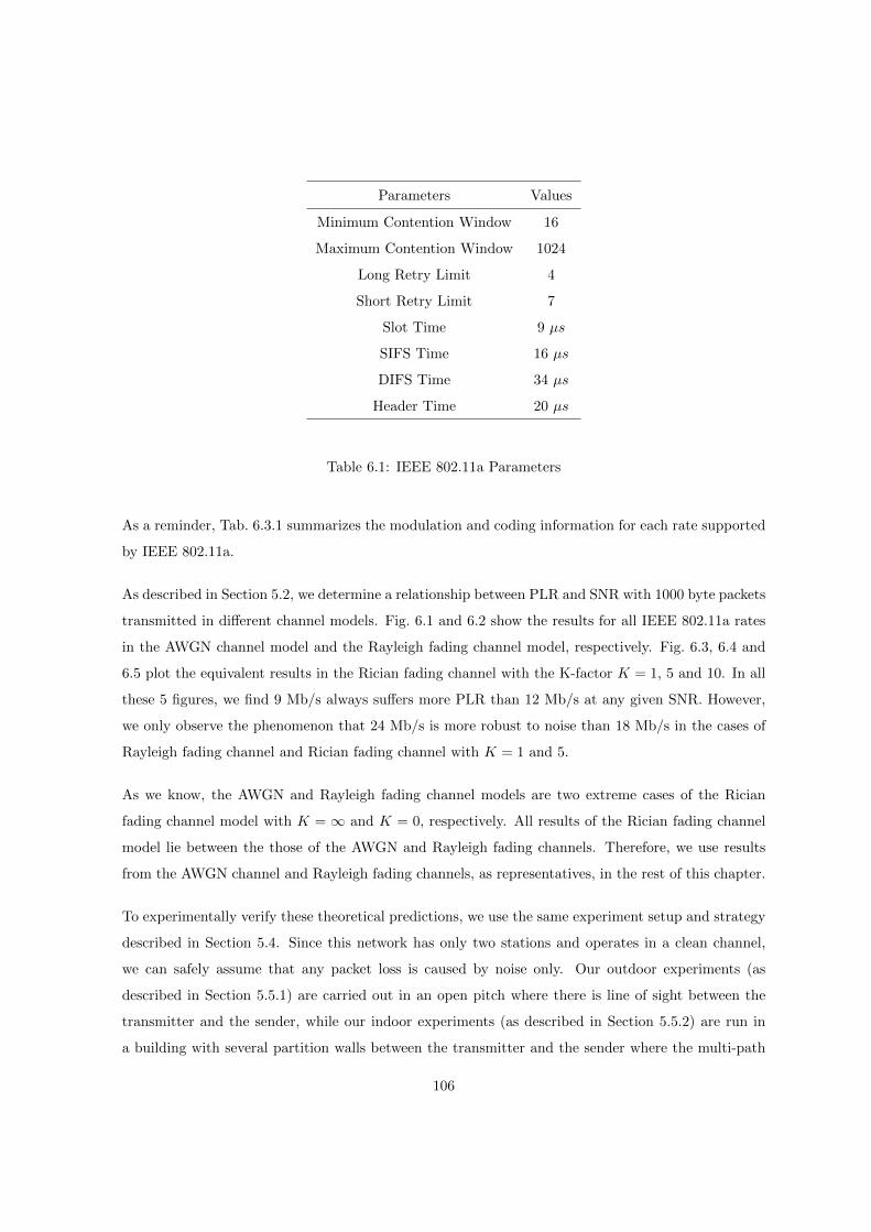
Parameters Values

Minimum Contention Window 16

Maximum Contention Window 1024

Long Retry Limit 4

Short Retry Limit 7

Slot Time 9 µs

SIFS Time 16 µs

DIFS Time 34 µs

Header Time 20 µs

Table 6.1: IEEE 802.11a Parameters

As a reminder, Tab. 6.3.1 summarizes the modulation and coding information for each rate supported

by IEEE 802.11a.

As described in Section 5.2, we determine a relationship between PLR and SNR with 1000 byte packets

transmitted in different channel models. Fig. 6.1 and 6.2 show the results for all IEEE 802.11a rates

in the AWGN channel model and the Rayleigh fading channel model, respectively. Fig. 6.3, 6.4 and

6.5 plot the equivalent results in the Rician fading channel with the K-factor K = 1, 5 and 10. In all

these 5 figures, we find 9 Mb/s always suffers more PLR than 12 Mb/s at any given SNR. However,

we only observe the phenomenon that 24 Mb/s is more robust to noise than 18 Mb/s in the cases of

Rayleigh fading channel and Rician fading channel with K = 1 and 5.

As we know, the AWGN and Rayleigh fading channel models are two extreme cases of the Rician

fading channel model with K = ∞ and K = 0, respectively. All results of the Rician fading channel

model lie between the those of the AWGN and Rayleigh fading channels. Therefore, we use results

from the AWGN channel and Rayleigh fading channels, as representatives, in the rest of this chapter.

To experimentally verify these theoretical predictions, we use the same experiment setup and strategy

described in Section 5.4. Since this network has only two stations and operates in a clean channel,

we can safely assume that any packet loss is caused by noise only. Our outdoor experiments (as

described in Section 5.5.1) are carried out in an open pitch where there is line of sight between the

transmitter and the sender, while our indoor experiments (as described in Section 5.5.2) are run in

a building with several partition walls between the transmitter and the sender where the multi-path

106

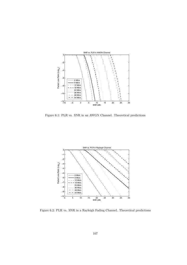
10 5 0 5 10 15 20 25 3012

10

8

6

4

2

0

SNR (dB)

Pack

et L

oss

Rat

io (L

og10

)

SNR vs. PLR in AWGN Channel


Figure 6.1: PLR vs. SNR in an AWGN Channel. Theoretical predictions

0 5 10 15 20 25 30 35 4010

9

8

7

6

5

4

3

2

1

0

SNR (dB)

Pack

et L

oss

Rat

io (L

og10

)

SNR vs. PLR in Rayleigh Channel


Figure 6.2: PLR vs. SNR in a Rayleigh Fading Channel. Theoretical predictions

107

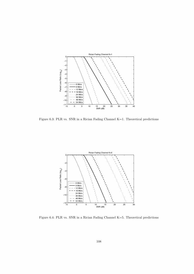
5 0 5 10 15 20 25 30 35 4011

10

9

8

7

6

5

4

3

2

1

0

SNR (dB)

Pack

et L

oss

Rat

io (L

og10

)



Figure 6.3: PLR vs. SNR in a Rician Fading Channel K=1. Theoretical predictions

5 0 5 10 15 20 25 3012

10

8

6

4

2

0

SNR (dB)

Pack

et L

oss

Rat

io (l

og10

)




108

10 5 0 5 10 15 20 25 3011

10

9

8

7

6

5

4

3

2

1

0

SNR (dB)

Pack

et L

oss

Rat

io (L

og10

)

Rician Fading Channel, K=10



propagation dominates. Therefore, we take the outdoor and indoor experiments as the representatives

of the AWGN channel model and Rayleigh fading channel model, respectively. In each experiment,

we broadcast 20,000 1000-byte packets from the transmitter to the receiver.

In both outdoor experiments and indoor experiments, define Lk := 1 if the kth transmission results

in a loss and Lk := 0 otherwise. First, we investigate the auto-covariance of the loss sequence {Lk}

of every IEEE 802.11a rate. As representative plots, Fig. 6.6 shows the auto-covariance for the loss

sequence at 12 Mb/s in the day-time outdoor environment, while Fig. 6.7 displays the auto-covariance

of the loss sequence at 12 Mb/s in the night-time indoor environments. The vertical range is extremely

small and suggests that packet losses occur stochastically pairwise independently.

Fig. 6.8 shows PLR vs. Transmission Rate for the outdoor experiments at a separation of 160 meters.

It shows 9 Mb/s suffers more losses than 12 Mb/s. Fig. 6.9 is the equivalent plot for the indoor

experiments in the night-time at a separation of 10 meters with several partition walls between them.

In the plot, it can be seen that the 9 Mb/s rate suffers a similar PLR to the 12 Mb/s rate. Note that

in these indoor experiments, where one might expect the Rayleigh fading model to be appropriate,

they do not confirm the second non-monotonic predictions of the Rayleigh fading channel model (18

Mb/s against 24 Mb/s).

A second collection of indoor experiments were performed at mid-day during a working week (an envi-

ronment in which H-RCA is supposed to work) to investigate the impact of channel conditions driven

109

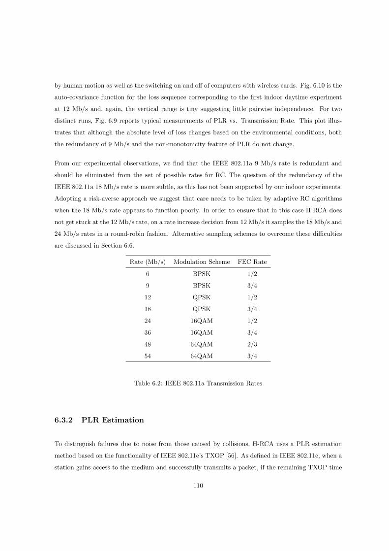
by human motion as well as the switching on and off of computers with wireless cards. Fig. 6.10 is the

auto-covariance function for the loss sequence corresponding to the first indoor daytime experiment

at 12 Mb/s and, again, the vertical range is tiny suggesting little pairwise independence. For two

distinct runs, Fig. 6.9 reports typical measurements of PLR vs. Transmission Rate. This plot illus-

trates that although the absolute level of loss changes based on the environmental conditions, both

the redundancy of 9 Mb/s and the non-monotonicity feature of PLR do not change.

From our experimental observations, we find that the IEEE 802.11a 9 Mb/s rate is redundant and

should be eliminated from the set of possible rates for RC. The question of the redundancy of the

IEEE 802.11a 18 Mb/s rate is more subtle, as this has not been supported by our indoor experiments.

Adopting a risk-averse approach we suggest that care needs to be taken by adaptive RC algorithms

when the 18 Mb/s rate appears to function poorly. In order to ensure that in this case H-RCA does

not get stuck at the 12 Mb/s rate, on a rate increase decision from 12 Mb/s it samples the 18 Mb/s and

24 Mb/s rates in a round-robin fashion. Alternative sampling schemes to overcome these difficulties

are discussed in Section 6.6.

Rate (Mb/s) Modulation Scheme FEC Rate

6 BPSK 1/2

9 BPSK 3/4

12 QPSK 1/2

18 QPSK 3/4

24 16QAM 1/2

36 16QAM 3/4

48 64QAM 2/3

54 64QAM 3/4

Table 6.2: IEEE 802.11a Transmission Rates

6.3.2 PLR Estimation

To distinguish failures due to noise from those caused by collisions, H-RCA uses a PLR estimation

method based on the functionality of IEEE 802.11e’s TXOP [56]. As defined in IEEE 802.11e, when a

station gains access to the medium and successfully transmits a packet, if the remaining TXOP time

110

0 20 40 60 80 100 120−0.1

−0.08

−0.06

−0.04

−0.02

0

0.02

0.04

0.06

0.08

0.1

Time Lag (seconds)

Auto−C

ovar

ianc

e

Figure 6.6: Auto-Covariance of the loss sequence of 12 Mb/s in the day-time outdoor environment at

160m separation. Experiment

0 10 20 30 40 50 600.1

0.08

0.06

0.04

0.02

0

0.02

0.04

0.06

0.08

0.1

Time Lag (seconds)

Auto

Cov

aria

nce

PLR=0.22

Figure 6.7: Auto-Covariance of the loss sequence of 12 Mb/s in the night-time indoor environment at

10m separation. Experiment

111

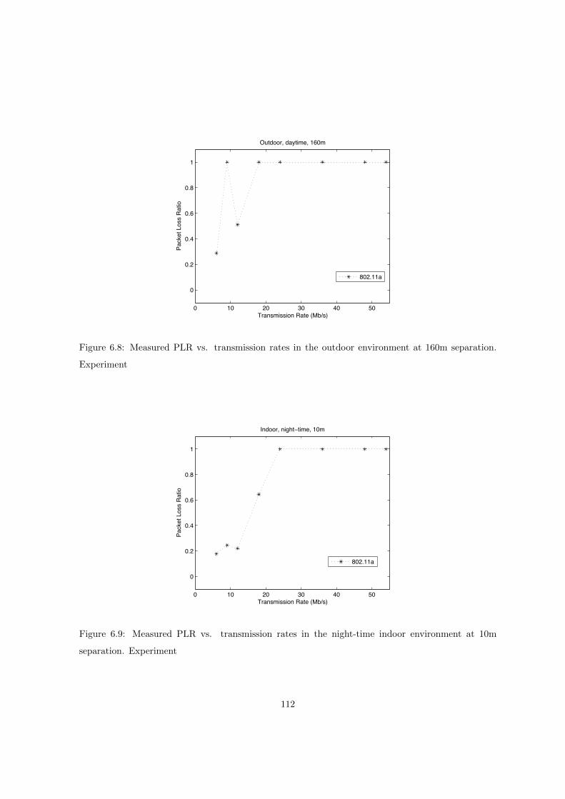
0 10 20 30 40 50

0

0.2

0.4

0.6

0.8

1


Pack

et L

oss

Rat

io

Outdoor, daytime, 160m

802.11a

Figure 6.8: Measured PLR vs. transmission rates in the outdoor environment at 160m separation.

Experiment

0 10 20 30 40 50

0

0.2

0.4

0.6

0.8

1


Pack

et L

oss

Rat

io

Indoor, night time, 10m

802.11a

Figure 6.9: Measured PLR vs. transmission rates in the night-time indoor environment at 10m

separation. Experiment

112

0 20 40 60 80 100 1200.1

0.08

0.06

0.04

0.02

0

0.02

0.04

0.06

0.08

0.1

Time Lag (seconds)

Auto

Cov

aria

nce

PLR=0.28

Figure 6.10: Auto-Covariance of the loss sequence of 12 Mb/s in the daytime indoor environment at

10m separation (1st experiment). Experiment

0 10 20 30 40 50

0

0.2

0.4

0.6

0.8

1


Indoor, daytime, 10m

Pack

et L

oss

Rat

io

1st run 802.11a2nd run 802.11a

Figure 6.11: Measured PLR vs. transmission rates in day-time indoor environment at 10m separation.

Experiment

113

is long enough for another packet transmission, the station can transmit the next packet after a short

inter-frame space (SIFS - see Appendix A) without an additional back-off period. If any packet in

the TXOP burst results in an unacknowledged transmission, no further packets are sent. At the time

the second or later packets in the TXOP burst are transmitted, all other stations in the network see

the medium as continuously busy so there can be no collision. In other words, if transmission of the

second or later packets in the TXOP burst fails, it can only have been caused by noise2. Transmission

failure of the first packet, however, can be due to both collision and noise. Thus it is necessary to

record transmission statistics for these two classes of packets.

Rate (Mb/s) TXOP (for 1kB packets) STh

6 0.0037s 742

12 0.0023s 1187

18 0.0018s 1497

24 0.0016s 1712

36 0.0014s 2037

48 0.0012s 2260

54 0.0012s N.A.

Table 6.3: IEEE 802.11a TXOP parameterization

In H-RCA, all packets are sent in TXOP bursts3. The TXOP value is rate and packet-size dependent.

It is set to allow two packets to be transmitted in each TXOP burst (for the IEEE 802.11a example,

see Tab. 6.3.2). For the sequence of first packets in the bursts, we define Fk := 1 if the kth first packet

is successfully received and Fk := 0 if it is not acknowledged by its intended receiver. For the sequence

of second packets in the TXOP bursts, which only exist if Fk = 1, we define Sk := 1 if the kth second

packet is successfully received and Sk := 0 otherwise. During time periods that rate change decisions

are made, which will be shown to be short, we assume that {Sk} forms an i.i.d. sequence. Based on,

for example, Fig. 6.6, Fig. 6.7 and Fig. 6.10, this is a reasonable hypothesis. Define

P (Sk = 0) := pn,

where pn is the probability of failure due to noise. Again, during the short time intervals during which

rate change decisions are made, we assume that {Fk} is i.i.d. and that collisions are independent of

2Losses due to hidden nodes are not considered directly in this chapter, see Section 6.6.43The question of lightly loaded stations is addressed in Section 6.6.

114

noise, so that

P (Fk = 0) = 1− (1− pn)(1− pc) =: pl,

where pc is the probability of failure due to collision and pl is the probability of failure due to either

collision or noise.

Ideally, H-RCA would only make its rate change decisions based on the sequence {Sk}, but it is

possible that this sequence will be completely censored by transmission failures of the first packets in

each TXOP burst (when P (Fk = 1) = 0). Thus a principled strategy is required to make decisions

based on the statistics of the first packets too.

6.3.3 Rate Reduction Decision

The fundamental goal of H-RCA is to minimize the average time that packets spend occupying the

medium, a quantity that we now determine as a function of MAC parameters, average packet size,

pn and pc. Define Ttx(r) to be the time on the medium of a first packet in a TXOP burst during a

transmission with a physical layer (PHY) rate r Mb/s. Then

Ttx(r) = DIFS+Header+(Payload)/r+SIFS+Header+ACK/rack,

where DIFS is the DCF inter-frame spacing, SIFS is the short inter-frame spacing and rack is the rate

at which the ACK is sent. In ns-2 rack is set to 1 Mb/s and can be regarded as a worst-case estimate.

In IEEE 802.11a experimental apparatus, rack is 6 Mb/s for the 6 and 9 Mb/s rates, 12 Mb/s for the

12 and 18 Mb/s rates, and 18 Mb/s for all higher rates. In H-RCA, all the re-transmissions proceed

with the current rate r with Multiple Rate Retry mechanism disabled. From the above assumptions,

using analysis along the lines found in [94], if a packet is the first packet in a TXOP burst and the

PHY rate is r Mb/s, its expected time on the medium is 4

M∑i=0

pilTtx(r) =1− pM+1

l

1− plTtx(r), (6.1)

where M is the IEEE 802.11 retry limit (see Appendix A). If a packet is the second in a TXOP burst,

its first transmission is delayed by a SIFS rather than a DIFS, where SIFS is two idle slots (σ) shorter

than DIFS, SIFS = DIFS-2σµs. Should it experience a collision, which can only be due to noise, it

4If successful and failed transmissions take distinct times, this can readily be taken into account.

115

becomes the first packet in the next TXOP burst, but can at most experience M − 1 more collisions

before being discarded. Thus at rate r Mb/s the expected time on the medium is

Ttx(r)− 2σ + pn

M−1∑i=0

pilTtx(r) (6.2)

= Ttx(r)− 2σ + pn1− pMl1− pl

Ttx(r).

These two expected waiting times have to be weighted based on the likelihood that when a packet is

first transmitted it is the first or second packet in a TXOP burst. These two events are not equally

likely as if a second packet in a TXOP burst experiences transmission failure, it becomes the first

packet in the next burst.

Under the above assumptions, the stochastic process that determines whether a packet is initially a

first or second packet in a TXOP burst forms a Markov chain on two states. The first state corresponds

to a packet initially being a first packet and the second corresponds to it initially being a second packet.

The Markov chain’s transition matrix is

Π =

pM+1l 1− pM+1

l

1− pn(1− pMl ) pn(1− pMl )

.

The entries of Π can be understood as follows: if a packet is initially the first packet in a TXOP burst,

the next one will also be the first packet if it is discarded, which happens with probability pM+1l . If

a packet is initially a second packet in a TXOP burst and it experiences a failed transmission due to

noise, it becomes a first packet and is then not discarded, which happens with probability pn(1−pMl ),

then the next packet will be a second packet too. The stationary distribution, λ where λΠ = λ, of

this Markov chain gives the long term probability that a packet is initially a first packet in a TXOP

burst or a second one: (1− pn(1− pMl )

2− pM+1l − pn(1− pMl )

,1− pM+1

l

2− pM+1l − pn(1− pMl )

).

Thus, with PHY rate r Mb/s, the average time that a packet spends being transmitted is

Ts(r) =1− pn(1− pMl )

2− pM+1l − pn(1− pMl )

(1− pM+1

l

1− plTtx(r)

)+ (6.3)

1− pM+1l

2− pM+1l − pn(1− pMl )

(Ttx(r)− 2σ + pn

1− pMl1− pl

Ttx(r)

).

For a given rate and channel model, the probability of loss due to noise pn can be determined as a

function of SNR.

116

Rate-reduction (IEEE 802.11a)

In Fig. 6.12 the channel is AWGN and the probability of transmission failure due to collision is

pc = 0.3, corresponding to a station competing with 6 stations that always have packets to send [19].

In Fig. 6.13 the channel is Rayleigh Fading and pc = 0.01, corresponding to a station competing for

access in a lightly loaded network [94]. These figures are representative of graphs for the AWGN and

Rayleigh fading channels and a wide range of conditional collision probabilities. In both figures, the

rate with the lowest average transmission time is the optimal rate for H-RCA at that SNR value. The

cross-points between these lines are the critical points where H-RCA should change its rate.

Corresponding to Figs 6.12 and 6.13, in terms of pn (log10 scale) vs. SNR, Figs 6.14 and 6.15 plot these

crossing-points. In both figures it is clear that those cross-points are distributed around the value

pn = 0.1. This pattern is the same for a wide range of conditional collision probabilities irrespective

of the channel model and, therefore, for convenience with the IEEE 802.11a rate-set, H-RCA uses

pn > 0.1 = pthresh as the threshold to trigger rate reduction at all rates. H-RCA could, of course,

be set up with a distinct pn threshold value for each rate. In selecting 0.1, we are typically erring on

the conservative side and demonstrate that this does not come at a significant performance cost. For

each rate, the average transmission time at the SNR corresponding to the threshold value pthresh is

indicated in Fig. 6.12 and 6.13.

The value pthresh = 0.1 is also suitable for the Rician fading channel with a wide range of K-factors

and conditional collision probabilities. Fig. 6.16, 6.17 and 6.18 show the cross-points in the Rician

fading channel with K = 1, 5 and 10, while pc = 0.2, 0.01 and 0.1. The corresponding average

transmission time at the SNR corresponding to the threshold value pthresh is plotted in Fig. 6.19, 6.20

and 6.21.

6.3.4 Rate-reduction: Bayesian inference

Based on observations of {Fk} and {Sk}, we adopt a Bayesian paradigm to the rate lowering decision.

First note that the statistics of {Fk} depend on pc as well as pn, while {Sk} only depends on pn.

Given a sufficient number of observations of {Sk} to enable a good estimate of pn, it is possible to

estimate pc from {Fk}. However, this is not an approach we use as if pn is large, it is possible that

we get no {Sk} observations.

117

Instead we will take a rate lowering decision based on the experience of either {Fk} or {Sk}, but

use a worst-case a priori upper bound on pc for {Fk} based on Bianchi’s well-known model [19].

Assuming that all stations always have packets to send, Fig. 6.22 plots Bianchi’s relationship between

the conditional collision probability, pc, and the number of stations in the WLAN. In practice, a

WLAN is not likely to have a network with over 40 stations that always have packets to send. For

such a situation, pc = 0.6 (the star point in Fig. 6.22). Thus, assuming pc = 0.6, H-RCA finds the

transmission failure probability, pl, of the first packet in the TXOP burst over 1− (1− 0.6)(1− p) =

0.6 + 0.4p then pn > p and it should choose a lower rate. For example, for the IEEE 802.11a rate-set

with p = 0.1, this value is pl = 0.64.

The Bayesian decision to change rate is based on the following question: using a uniform prior for

pn on [0, 1], conditional on the fact that the noise packet loss probability, pn, is over p, in N packet

transmissions, the Bayesian sampling window, how many failures should be observed before H-RCA

has over 95% confidence that pn > p? With pl(pc, pn) := 1 − (1 − pc)(1 − pn) and pc known, this

corresponds to finding the minimal value of I that satisfies the following inequality:∫ 1

p

(N

I

)(1− pl(pc, pn))N−Ipl(pc, pn)I dpn∫ 1

0

(N

I

)(1− pl(pc, pn))N−Ipl(pc, pn)I dpn

≥ 0.95. (6.4)

Bayesian inference (IEEE 802.11a)

Using (6.4), out of N = 50 transmission samples for each sequence, {Fk} and {Sk}, and assuming

pc = 0.6 for {Fk} and pc = 0 for {Sk}, H-RCA should observe at least 39 failures out of 50 first

packet transmissions or 9 failures out of 50 second packet transmissions to be over 95% confident that

the pn > 0.1 for the current rate and to decide to choose a lower rate. Note that these numbers,

based on a principled design, are efficient. If the noise probability pn is small enough that a rate

reduction decision is not taken based on F1, . . . , FN , then we will quickly get a sufficient sample of

second packets in order to make an accurate decision based on noise-only failures. On the other hand,

if the WLAN has less than 40 stations that always have packets to send and H-RCA sees more than

39 transmission failures for 50 first packets, it can confidently decide that pn > 0.1 and lower the

transmission rate.

118

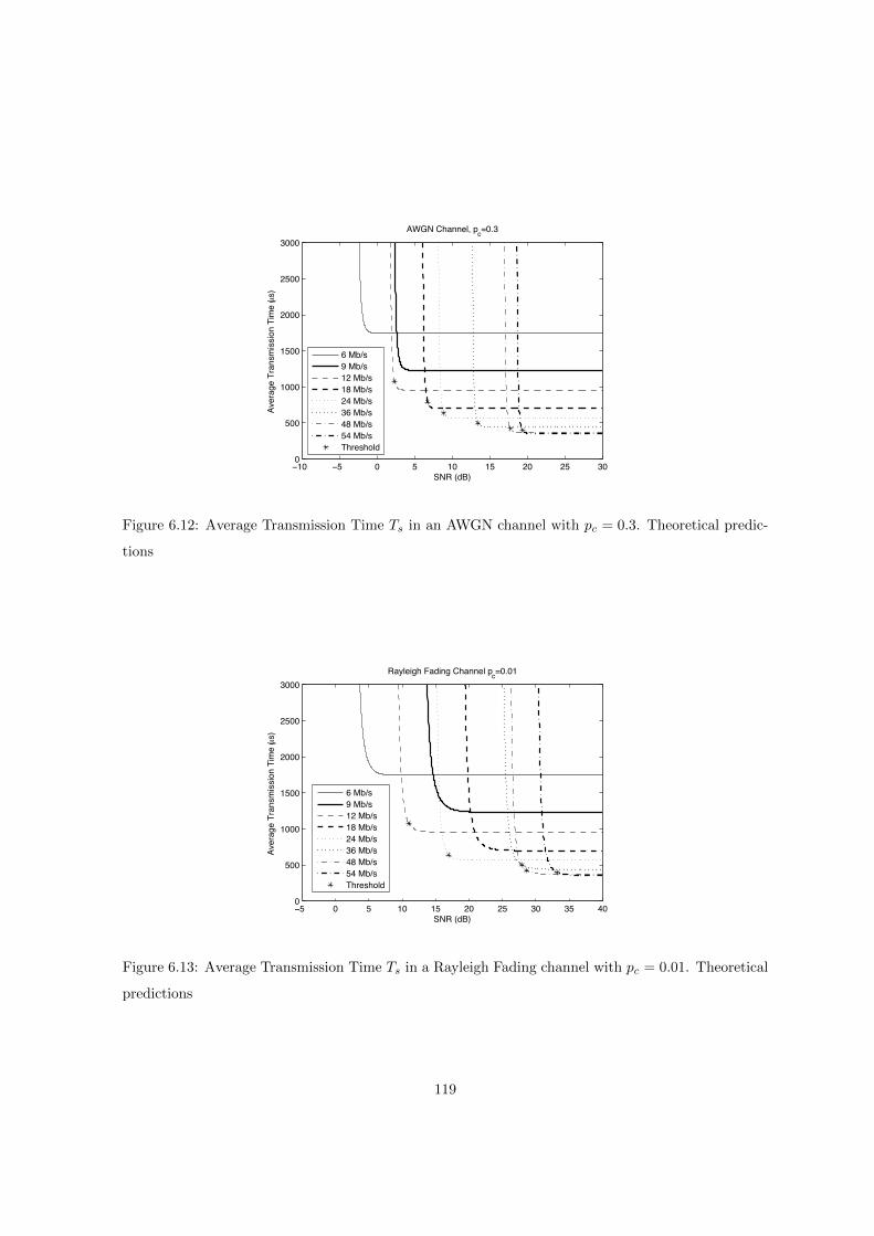
10 5 0 5 10 15 20 25 300

500

1000

1500

2000

2500

3000

SNR (dB)

Aver

age

Tran

smis

sion

Tim

e (µs

)

AWGN Channel, pc=0.3

6 Mb/s9 Mb/s12 Mb/s18 Mb/s24 Mb/s36 Mb/s48 Mb/s54 Mb/sThreshold

Figure 6.12: Average Transmission Time Ts in an AWGN channel with pc = 0.3. Theoretical predic-

tions

5 0 5 10 15 20 25 30 35 400

500

1000

1500

2000

2500

3000

SNR (dB)

Aver

age

Tran

smis

sion

Tim

e (µs

)

Rayleigh Fading Channel pc=0.01


Figure 6.13: Average Transmission Time Ts in a Rayleigh Fading channel with pc = 0.01. Theoretical

predictions

119

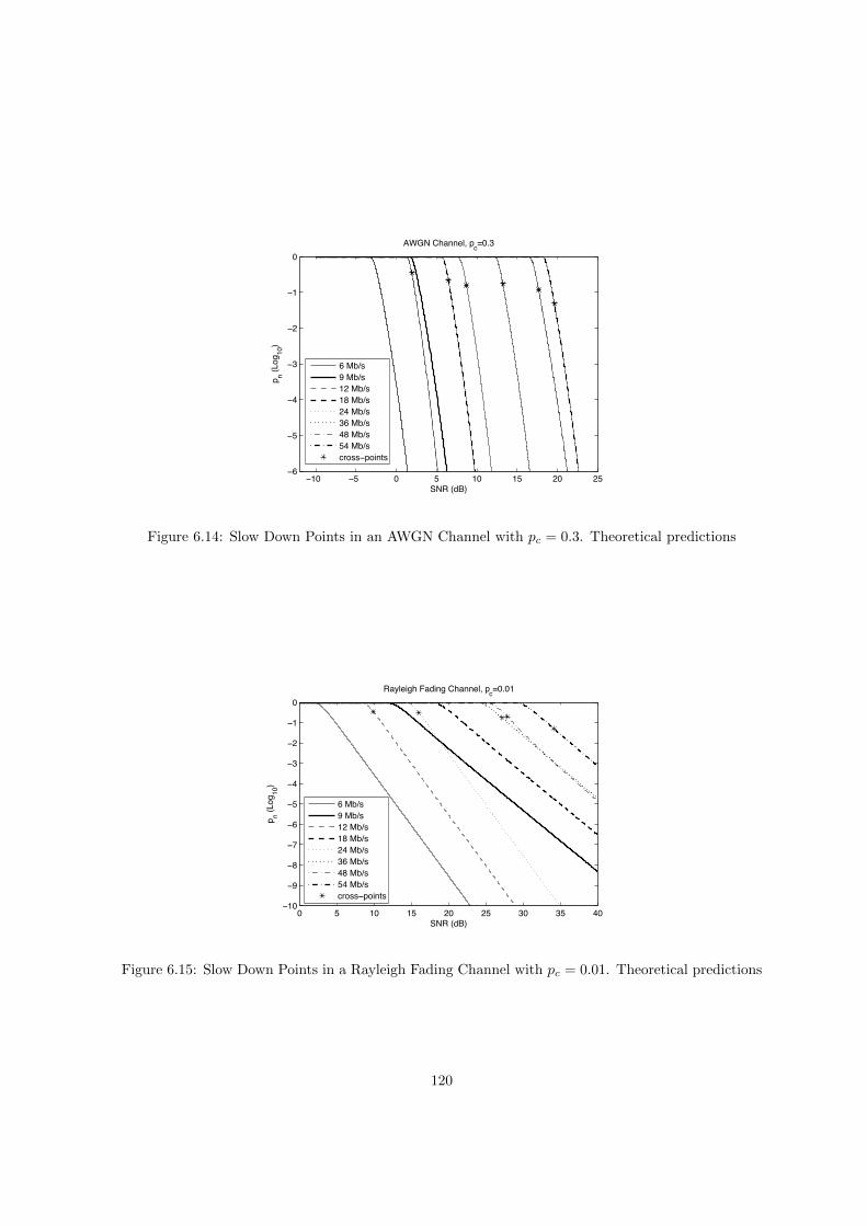
10 5 0 5 10 15 20 256

5

4

3

2

1

0

SNR (dB)

p n (Log

10)

AWGN Channel, pc=0.3

6 Mb/s9 Mb/s12 Mb/s18 Mb/s24 Mb/s36 Mb/s48 Mb/s54 Mb/scross points

Figure 6.14: Slow Down Points in an AWGN Channel with pc = 0.3. Theoretical predictions

0 5 10 15 20 25 30 35 4010

9

8

7

6

5

4

3

2

1

0

SNR (dB)

p n (Log

10)

Rayleigh Fading Channel, pc=0.01


Figure 6.15: Slow Down Points in a Rayleigh Fading Channel with pc = 0.01. Theoretical predictions

120

10 5 0 5 10 15 20 25 306

5

4

3

2

1

0

SNR (dB)

p n(log 10

)

Rician Fading Channel K=1 pc=0.2


Figure 6.16: Slow Down Points in a Rician fading channelK = 1 with pc = 0.2. Theoretical predictions

10 5 0 5 10 15 20 25 306

5

4

3

2

1

0

SNR (dB)

Pack

et L

oss

Rat

io (l

og10

)



Figure 6.17: Slow Down Points in a Rician fading channel K = 5 with pc = 0.01. Theoretical

predictions

121

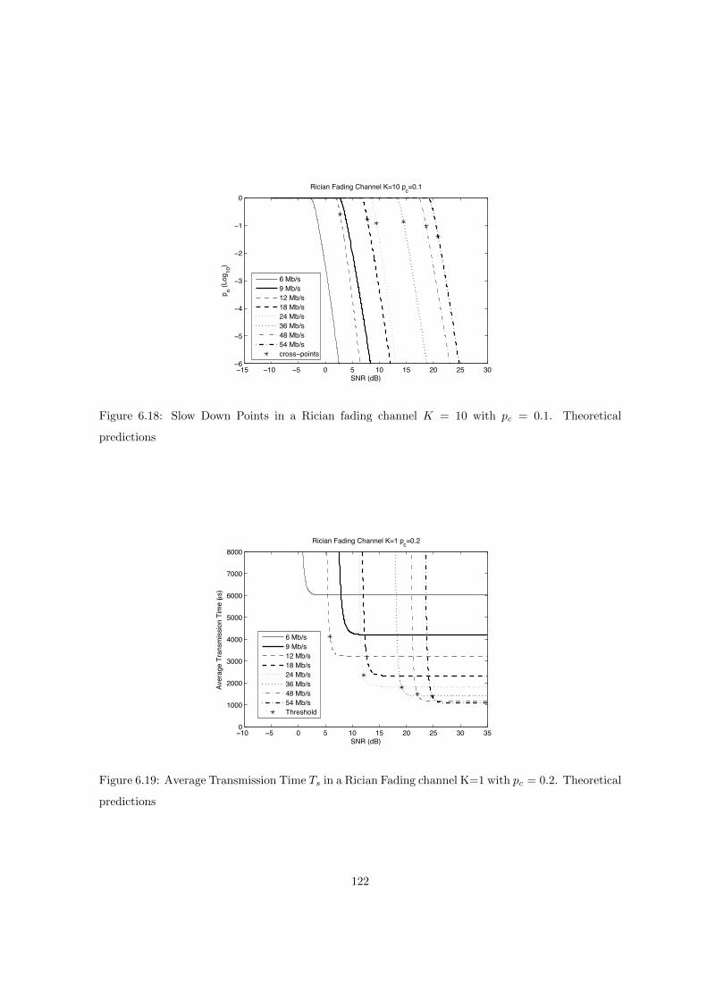
15 10 5 0 5 10 15 20 25 306

5

4

3

2

1

0

SNR (dB)

p n (Log

10)



Figure 6.18: Slow Down Points in a Rician fading channel K = 10 with pc = 0.1. Theoretical

predictions

10 5 0 5 10 15 20 25 30 350

1000

2000

3000

4000

5000

6000

7000

8000

SNR (dB)

Aver

age

Tran

smis

sion

Tim

e (µs

)



Figure 6.19: Average Transmission Time Ts in a Rician Fading channel K=1 with pc = 0.2. Theoretical

predictions

122

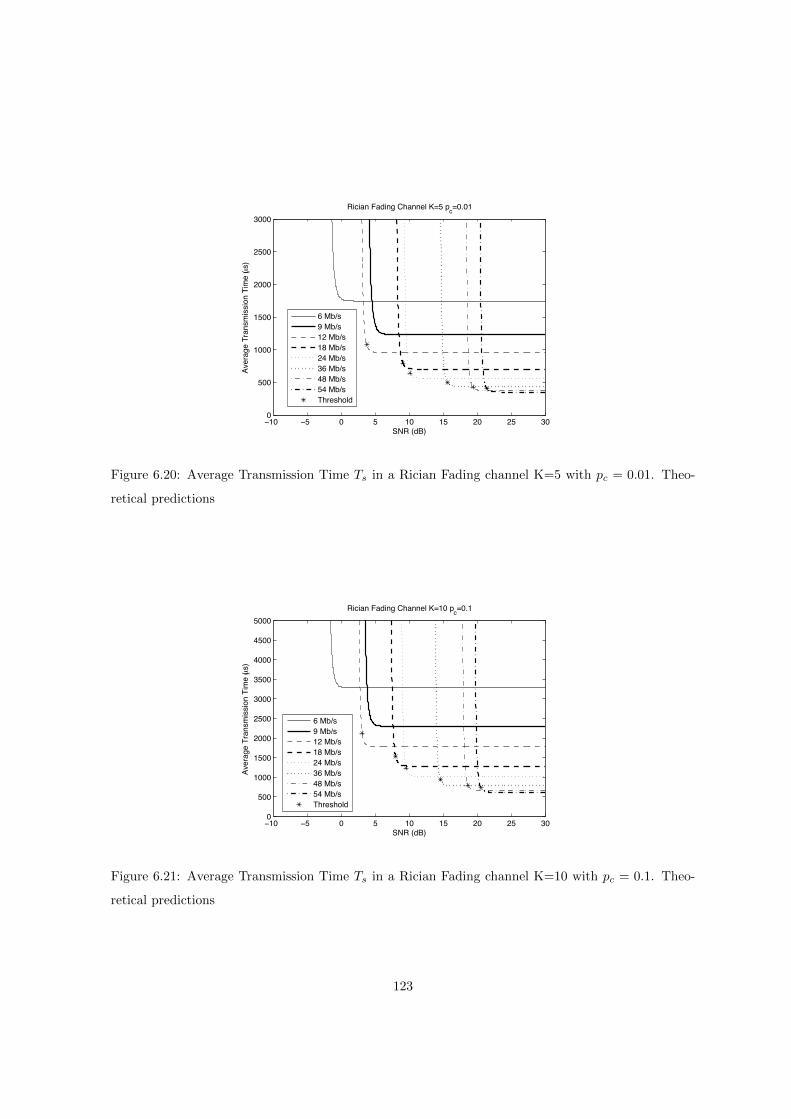
10 5 0 5 10 15 20 25 300

500

1000

1500

2000

2500

3000

SNR (dB)

Aver

age

Tran

smis

sion

Tim

e (µs

)



Figure 6.20: Average Transmission Time Ts in a Rician Fading channel K=5 with pc = 0.01. Theo-

retical predictions

10 5 0 5 10 15 20 25 300

500

1000

1500

2000

2500

3000

3500

4000

4500

5000

SNR (dB)

Aver

age

Tran

smis

sion

Tim

e (µs

)



Figure 6.21: Average Transmission Time Ts in a Rician Fading channel K=10 with pc = 0.1. Theo-

retical predictions

123

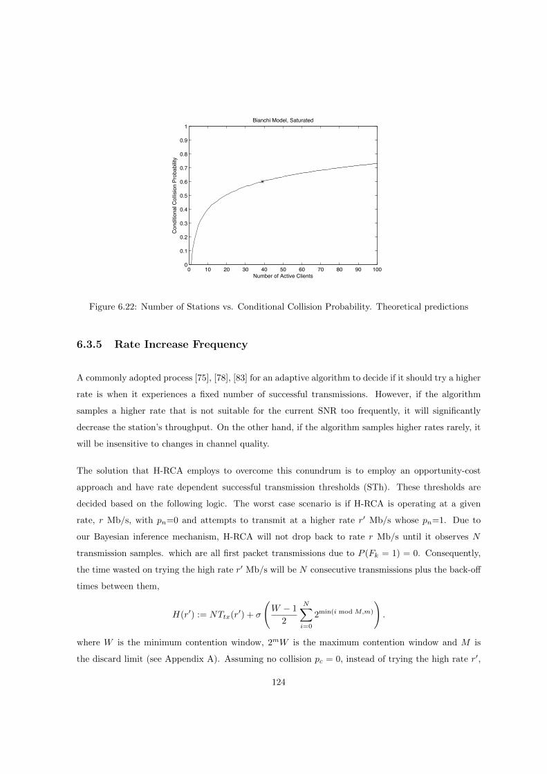
0 10 20 30 40 50 60 70 80 90 1000

0.1

0.2

0.3

0.4

0.5

0.6

0.7

0.8

0.9

1

Number of Active Clients

Cond

itiona

l Col

lisio

n Pr

obab

ility

Bianchi Model, Saturated

Figure 6.22: Number of Stations vs. Conditional Collision Probability. Theoretical predictions

6.3.5 Rate Increase Frequency

A commonly adopted process [75], [78], [83] for an adaptive algorithm to decide if it should try a higher

rate is when it experiences a fixed number of successful transmissions. However, if the algorithm

samples a higher rate that is not suitable for the current SNR too frequently, it will significantly

decrease the station’s throughput. On the other hand, if the algorithm samples higher rates rarely, it

will be insensitive to changes in channel quality.

The solution that H-RCA employs to overcome this conundrum is to employ an opportunity-cost

approach and have rate dependent successful transmission thresholds (STh). These thresholds are

decided based on the following logic. The worst case scenario is if H-RCA is operating at a given

rate, r Mb/s, with pn=0 and attempts to transmit at a higher rate r′ Mb/s whose pn=1. Due to

our Bayesian inference mechanism, H-RCA will not drop back to rate r Mb/s until it observes N

transmission samples. which are all first packet transmissions due to P (Fk = 1) = 0. Consequently,

the time wasted on trying the high rate r′ Mb/s will be N consecutive transmissions plus the back-off

times between them,

H(r′) := NTtx(r′) + σ

(W − 1

2

N∑i=0

2min(i mod M,m)

).

where W is the minimum contention window, 2mW is the maximum contention window and M is

the discard limit (see Appendix A). Assuming no collision pc = 0, instead of trying the high rate r′,

124

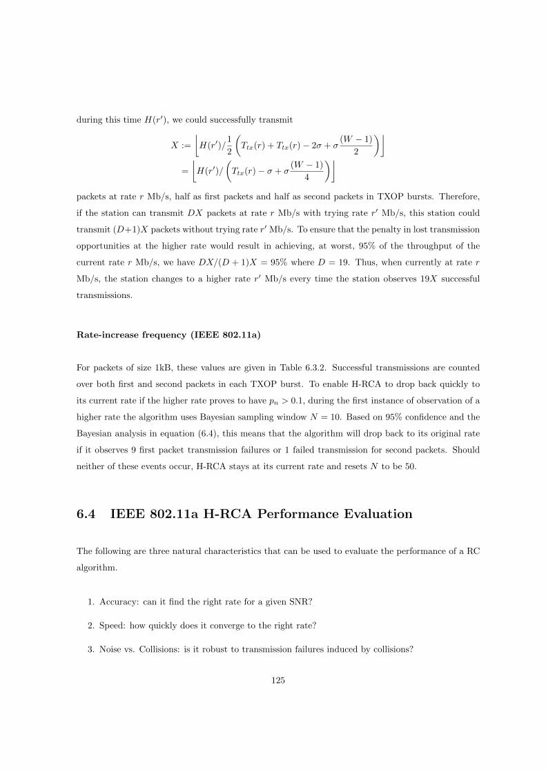
during this time H(r′), we could successfully transmit

X :=

⌊H(r′)/

1

2

(Ttx(r) + Ttx(r)− 2σ + σ

(W − 1)

2

)⌋=

⌊H(r′)/

(Ttx(r)− σ + σ

(W − 1)

4

)⌋packets at rate r Mb/s, half as first packets and half as second packets in TXOP bursts. Therefore,

if the station can transmit DX packets at rate r Mb/s with trying rate r′ Mb/s, this station could

transmit (D+1)X packets without trying rate r′ Mb/s. To ensure that the penalty in lost transmission

opportunities at the higher rate would result in achieving, at worst, 95% of the throughput of the

current rate r Mb/s, we have DX/(D + 1)X = 95% where D = 19. Thus, when currently at rate r

Mb/s, the station changes to a higher rate r′ Mb/s every time the station observes 19X successful

transmissions.

Rate-increase frequency (IEEE 802.11a)

For packets of size 1kB, these values are given in Table 6.3.2. Successful transmissions are counted

over both first and second packets in each TXOP burst. To enable H-RCA to drop back quickly to

its current rate if the higher rate proves to have pn > 0.1, during the first instance of observation of a

higher rate the algorithm uses Bayesian sampling window N = 10. Based on 95% confidence and the

Bayesian analysis in equation (6.4), this means that the algorithm will drop back to its original rate

if it observes 9 first packet transmission failures or 1 failed transmission for second packets. Should

neither of these events occur, H-RCA stays at its current rate and resets N to be 50.

6.4 IEEE 802.11a H-RCA Performance Evaluation

The following are three natural characteristics that can be used to evaluate the performance of a RC

algorithm.

1. Accuracy: can it find the right rate for a given SNR?

2. Speed: how quickly does it converge to the right rate?

3. Noise vs. Collisions: is it robust to transmission failures induced by collisions?

125

As it is challenging to build an experimental wireless channel with controllable noise characteristics,

here we first present results from ns-2 simulations. Data from an experimental implementation is

reported in Section 6.5. In simulation we used both the AWGN and Rayleigh Fading channel models

to determine pn, the probability of failure due to noise, at each rate at a given SNR.

In existing commodity hardware, the physical layer performs automatic re-sends on transmission

failure and the network card driver is only made aware of the transmission result at the MAC layer.

To mirror this constraint, in ns-2 H-RCA works on information at the MAC-level, so H-RCA is

only informed of the totality of a packet’s transmission results after it has been successfully sent or

discarded. That is, H-RCA receives new data only when the MAC layer finishes servicing each packet.

All stations transmit fixed 1kB UDP packets to an Access Point (AP) and always have packets to

send. H-RCA’s TXOP and STh values are set as in Tab. 6.3.2. We have also implemented SampleRate

[22] in ns-2. In order to provide a fair comparison we use the same simulation settings, including the

same rate-set, TXOP values and the redundant 9 Mb/s rate is excluded from SampleRate’s rate list.

We perform two sets of simulations to determine accuracy and speed. One set has a single station, so

there are no collisions. The second set has five stations so that transmission failure can be caused by

collisions.

We report on H-RCA’s performance under two distinct, evolving SNR conditions: 1. step changes in

channel quality; 2. gradual changes in channel quality. In the step-change case, SNR changes with

the following discontinuous function:

SNR(t) =

(15 +G(t)) dB if 0s ≤ t ≤ 300s

(10 +G(t)) dB if 300s < t ≤ 600s

(5 +G(t)) dB if 600s < t ≤ 1200s

(10 +G(t)) dB if 1200s < t ≤ 1500s

(15 +G(t)) dB if 1500s < t ≤ 1800s

While in the gradient-change case, SNR varies as the following continuous V-shaped function:

SNR(t) =

(

15− t

90+G(t)

)dB if 0 ≤ t ≤ 900s(

−5 +t

90+G(t)

)dB if 900s < t ≤ 1800s

In both cases, {G(t)} is Gaussian Process with mean 0 and variance 1 and the resulting pn is deter-

mined from the AWGN channel model and the Rayleigh fading channel model.

126

6.4.1 Single Station, No Collisions

Our first simulation takes place in a WLAN with a single active client so that it experiences no

collisions. In the discontinuous SNR scenario, Fig. 6.23 and Fig. 6.24 show the WLAN’s second-

by-second throughput when using either H-RCA or SampleRate in an AWGN channel model and a

Rayleigh fading channel model, respectively. In both graphs the boxes in the top left corner give the

30-minute average throughput for each RC algorithm and show that H-RCA gets higher throughput

than SampleRate. In the Rayleigh fading channel (Fig. 6.24), the throughput of SampleRate is only

62% of the one provided by H-RCA. In Fig. 6.24, we also observed that SampleRate can not make

the right decision for some time, for example, when SNR is around 15dB and 5dB. SampleRate loses

throughput as it frequently samples the whole rate space, which seriously reduces throughput. H-

RCA’s sampling frequency is restricted by design, so it achieves a consistently higher throughput

than SampleRate. To show the benefit of limiting the sampling frequency in H-RCA, in the case

of the AWGN channel, we also implemented an omniscient optimal algorithm that knows channel

conditions in advance and can select the best rate at all times based on Fig.6.14. Comparisons with

this omniscient algorithm shows that H-RCA is accurate, finding the correct rate and sampling the

one above it. In this AWGN case, the 30-minute average throughput of the omniscient algorithm is 9.2

Mb/s, while H-RCA gets 97% of this figure, as one would expect based on its rate-increase opportunity

cost paradigm. In addition, both figures show that H-RCA is responsive to a sudden change in SNR

where it only takes seconds to adapt and stabilize the rate in response to the dramatically different

environmental conditions.

Fig. 6.25 and Fig. 6.26 show simulation results in the case of SNR gradient in both two channel models,

which demonstrates that H-RCA still delivers greater and less variable throughput than SampleRate.

In both figures, H-RCA sustains network throughput when SNR decreases slowly (from 200s to 600s),

while the throughput of SampleRate drops continuously and is highly variable. Sizable drops in

SampleRate’s throughput flag instances when SampleRate adapts its rate. H-RCA, however, makes

better decisions more quickly and more accurately.

As examples to show the H-RCA’s decision making process, Fig. 6.27 displays the instances at which

rate change decisions were made in the example shown in Fig. 6.25, while Fig. 6.28 indicates the

rate-change event in the example shown in Fig. 6.24. In both graphs, the event ‘UP’ means H-RCA

decides to sample the higher rate, the event ‘FFTh’ means H-RCA decides to decrease its rate based

on the observations of the first packets in the TXOP bursts, {Fk}, and the event ‘SFTh’ means H-

127

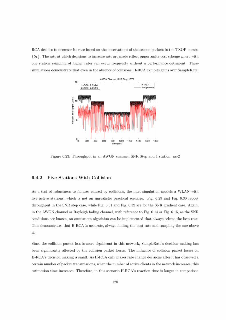
RCA decides to decrease its rate based on the observations of the second packets in the TXOP bursts,

{Sk}. The rate at which decisions to increase rate are made reflect opportunity cost scheme where with

one station sampling of higher rates can occur frequently without a performance detriment. These

simulations demonstrate that even in the absence of collisions, H-RCA exhibits gains over SampleRate.

0 200 400 600 800 1000 1200 1400 1600 18000

5

10

15

Time (sec)

Net

wor

k Th

roug

hput

(Mb/

s)

AWGN Channel, SNR Step, 1STA

H−RCASampleRate

H−RCA: 9.0 Mb/sSample: 6.2 Mb/s

Figure 6.23: Throughput in an AWGN channel, SNR Step and 1 station. ns-2

6.4.2 Five Stations With Collision

As a test of robustness to failures caused by collisions, the next simulation models a WLAN with

five active stations, which is not an unrealistic practical scenario. Fig. 6.29 and Fig. 6.30 report

throughput in the SNR step case, while Fig. 6.31 and Fig. 6.32 are for the SNR gradient case. Again,

in the AWGN channel or Rayleigh fading channel, with reference to Fig. 6.14 or Fig. 6.15, as the SNR

conditions are known, an omniscient algorithm can be implemented that always selects the best rate.

This demonstrates that H-RCA is accurate, always finding the best rate and sampling the one above

it.

Since the collision packet loss is more significant in this network, SampleRate’s decision making has

been significantly affected by the collision packet losses. The influence of collision packet losses on

H-RCA’s decision making is small. As H-RCA only makes rate change decisions after it has observed a

certain number of packet transmissions, when the number of active clients in the network increases, this

estimation time increases. Therefore, in this scenario H-RCA’s reaction time is longer in comparison

128

0 200 400 600 800 1000 1200 1400 1600 18000

2

4

6

8

10

12

Time (sec)

Net

wor

k Th

roug

hput

(Mb/

s)

Rayleigh Fading Channel, SNR Step, 1STA

H−RCASampleRate

H−RCA: 6.3 Mb/sSampleRate: 3.9 Mb/s

Figure 6.24: Throughput in a Rayleigh fading channel, SNR Step and 1 station. ns-2

0 200 400 600 800 1000 1200 1400 1600 18000

2

4

6

8

10

12

14

Time (sec)

Net

wor

k Th

roug

hput

(Mb/

s)

AWGN Channel, SNR Gradient, 1STA

H−RCASampleRate


Figure 6.25: Throughput in an AWGN channel, SNR Gradient and 1 station. ns-2

129

0 200 400 600 800 1000 1200 1400 1600 18000

1

2

3

4

5

6

7

8

9

10

11

Time (sec)

Net

wor

k Th

roug

hput

(Mb/

s)

Rayleigh Fading Channel, SNR Gradient, 1STA

H−RCASampleRate


Figure 6.26: Throughput in a Rayleigh fading channel, SNR Gradient and 1 station. ns-2

0 200 400 600 800 1000 1200 1400 1600 18000

5

10

15

20

25

30

35

40

45

50

55

Time (sec)

Rate

(Mb/

s)

AWGN Channel, SNR Gradient, 1STA

RATEUPFFThSFTh

Figure 6.27: Rate change decisions in an AWGN channel, SNR Gradient and 1 station. UP indicates

a rate increase decision, FFTh indicates a rate decrease decision based on first packets in a TXOP

burst and SFTh indicates a rate decrease decision based on second packets in a TXOP burst. ns-2

130

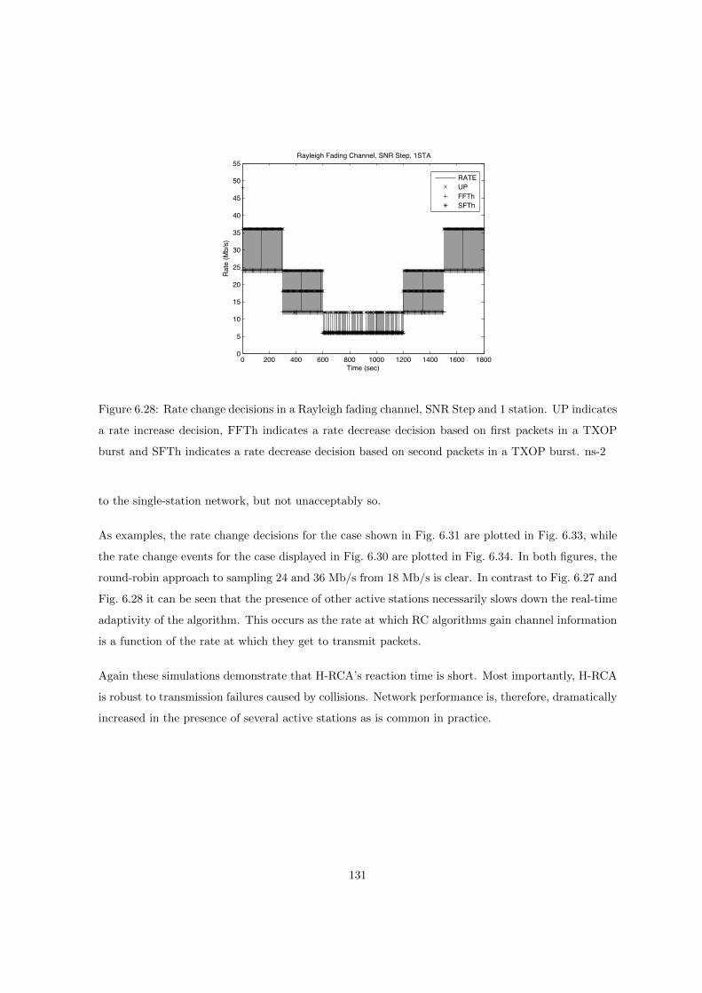
0 200 400 600 800 1000 1200 1400 1600 18000

5

10

15

20

25

30

35

40

45

50

55

Time (sec)

Rate

(Mb/

s)

Rayleigh Fading Channel, SNR Step, 1STA

RATEUPFFThSFTh

Figure 6.28: Rate change decisions in a Rayleigh fading channel, SNR Step and 1 station. UP indicates



to the single-station network, but not unacceptably so.

As examples, the rate change decisions for the case shown in Fig. 6.31 are plotted in Fig. 6.33, while

the rate change events for the case displayed in Fig. 6.30 are plotted in Fig. 6.34. In both figures, the

round-robin approach to sampling 24 and 36 Mb/s from 18 Mb/s is clear. In contrast to Fig. 6.27 and

Fig. 6.28 it can be seen that the presence of other active stations necessarily slows down the real-time

adaptivity of the algorithm. This occurs as the rate at which RC algorithms gain channel information

is a function of the rate at which they get to transmit packets.

Again these simulations demonstrate that H-RCA’s reaction time is short. Most importantly, H-RCA

is robust to transmission failures caused by collisions. Network performance is, therefore, dramatically

increased in the presence of several active stations as is common in practice.

131

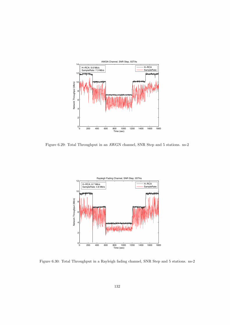
0 200 400 600 800 1000 1200 1400 1600 18000

2

4

6

8

10

12

14

Time (sec)

Net

wor

k Th

roug

hput

(Mb/

s)

AWGN Channel, SNR Step, 5STAs

H−RCASampleRate


Figure 6.29: Total Throughput in an AWGN channel, SNR Step and 5 stations. ns-2

0 200 400 600 800 1000 1200 1400 1600 18000

2

4

6

8

10

12

Time (sec)

Net

wor

k Th

roug

hput

(Mb/

s)

Rayleigh Fading Channel, SNR Step, 5STAs

H−RCASampleRate


Figure 6.30: Total Throughput in a Rayleigh fading channel, SNR Step and 5 stations. ns-2

132

0 200 400 600 800 1000 1200 1400 1600 18000

2

4

6

8

10

12

14

Time (sec)

Net

wor

k Th

roug

hput

(Mb/

s)

AWGN Channel, SNR Gradient, 5STAs

H−RCASampleRate


Figure 6.31: Total Throughput in an AWGN channel, SNR Gradient and 5 stations. ns-2

0 200 400 600 800 1000 1200 1400 1600 18000

2

4

6

8

10

12

Time (sec)

Net

wor

k Th

roug

hput

(Mb/

s)

Rayleigh Fading Channel, SNR Gradient, 5STAs

H−RCASampleRate


Figure 6.32: Total Throughput in a Rayleigh fading channel, SNR Gradient and 5 stations. ns-2

133

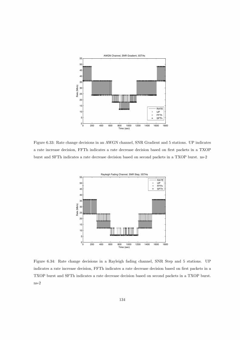
0 200 400 600 800 1000 1200 1400 1600 18000

5

10

15

20

25

30

35

40

45

50

55

Time (sec)

Rate

(Mb/

s)

AWGN Channel, SNR Gradient, 5STAs

RATEUPFFThSFTh

Figure 6.33: Rate change decisions in an AWGN channel, SNR Gradient and 5 stations. UP indicates



0 200 400 600 800 1000 1200 1400 1600 18000

5

10

15

20

25

30

35

40

45

50

55

Time (sec)

Rate

(Mb/

s)

Rayleigh Fading Channel, SNR Step, 5STAs

RATEUPFFThSFTh

Figure 6.34: Rate change decisions in a Rayleigh fading channel, SNR Step and 5 stations. UP

indicates a rate increase decision, FFTh indicates a rate decrease decision based on first packets in a

TXOP burst and SFTh indicates a rate decrease decision based on second packets in a TXOP burst.

ns-2

134

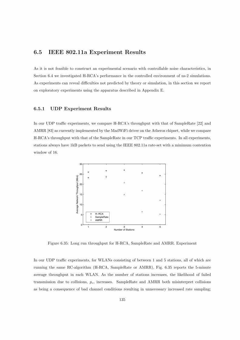
6.5 IEEE 802.11a Experiment Results

As it is not feasible to construct an experimental scenario with controllable noise characteristics, in

Section 6.4 we investigated H-RCA’s performance in the controlled environment of ns-2 simulations.

As experiments can reveal difficulties not predicted by theory or simulation, in this section we report

on exploratory experiments using the apparatus described in Appendix E.

6.5.1 UDP Experiment Results

In our UDP traffic experiments, we compare H-RCA’s throughput with that of SampleRate [22] and

AMRR [83] as currently implemented by the MadWiFi driver on the Atheros chipset, while we compare

H-RCA’s throughput with that of the SampleRate in our TCP traffic experiments. In all experiments,

stations always have 1kB packets to send using the IEEE 802.11a rate-set with a minimum contention

window of 16.

1 2 3 4 50

5

10

15

20

25

30

Number of Stations

Aver

age

Net

wor

k Th

roug

hput

(Mb/

s)

H−RCASampleRateAMRR

Figure 6.35: Long run throughput for H-RCA, SampleRate and AMRR. Experiment

In our UDP traffic experiments, for WLANs consisting of between 1 and 5 stations, all of which are

running the same RC-algorithm (H-RCA, SampleRate or AMRR), Fig. 6.35 reports the 5-minute

average throughput in each WLAN. As the number of stations increases, the likelihood of failed

transmission due to collisions, pc, increases. SampleRate and AMRR both misinterpret collisions

as being a consequence of bad channel conditions resulting in unnecessary increased rate sampling;

135

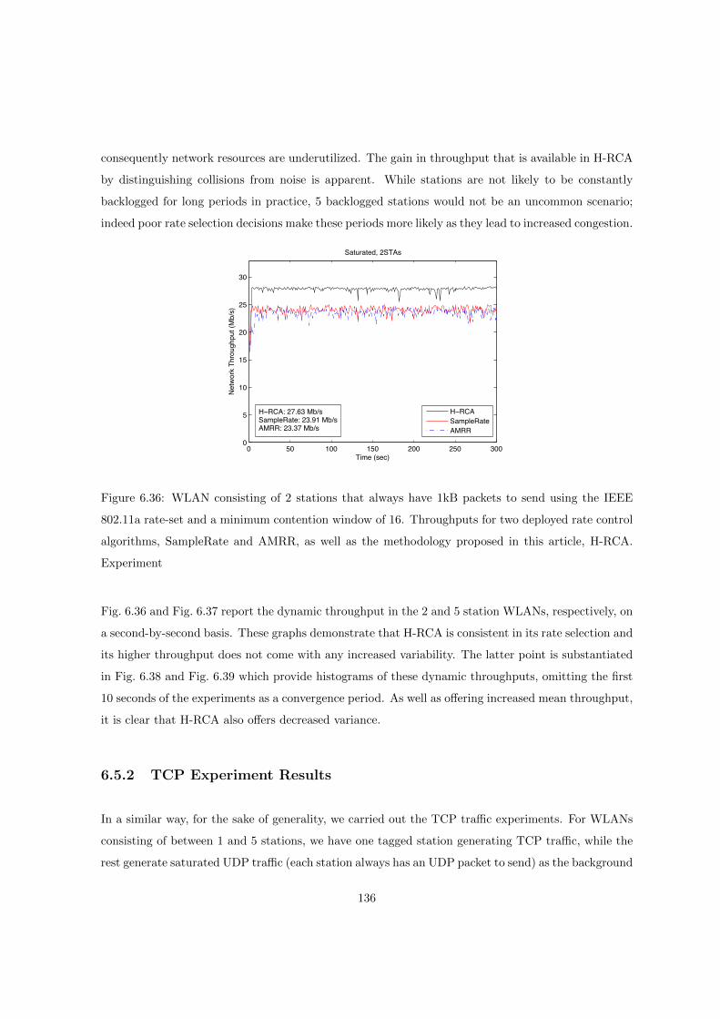
consequently network resources are underutilized. The gain in throughput that is available in H-RCA

by distinguishing collisions from noise is apparent. While stations are not likely to be constantly

backlogged for long periods in practice, 5 backlogged stations would not be an uncommon scenario;

indeed poor rate selection decisions make these periods more likely as they lead to increased congestion.

0 50 100 150 200 250 3000

5

10

15

20

25

30

Time (sec)

Net

wor

k Th

roug

hput

(Mb/

s)

Saturated, 2STAs


H−RCA: 27.63 Mb/sSampleRate: 23.91 Mb/sAMRR: 23.37 Mb/s

Figure 6.36: WLAN consisting of 2 stations that always have 1kB packets to send using the IEEE

802.11a rate-set and a minimum contention window of 16. Throughputs for two deployed rate control

algorithms, SampleRate and AMRR, as well as the methodology proposed in this article, H-RCA.

Experiment

Fig. 6.36 and Fig. 6.37 report the dynamic throughput in the 2 and 5 station WLANs, respectively, on

a second-by-second basis. These graphs demonstrate that H-RCA is consistent in its rate selection and

its higher throughput does not come with any increased variability. The latter point is substantiated

in Fig. 6.38 and Fig. 6.39 which provide histograms of these dynamic throughputs, omitting the first

10 seconds of the experiments as a convergence period. As well as offering increased mean throughput,

it is clear that H-RCA also offers decreased variance.

6.5.2 TCP Experiment Results

In a similar way, for the sake of generality, we carried out the TCP traffic experiments. For WLANs

consisting of between 1 and 5 stations, we have one tagged station generating TCP traffic, while the

rest generate saturated UDP traffic (each station always has an UDP packet to send) as the background

136

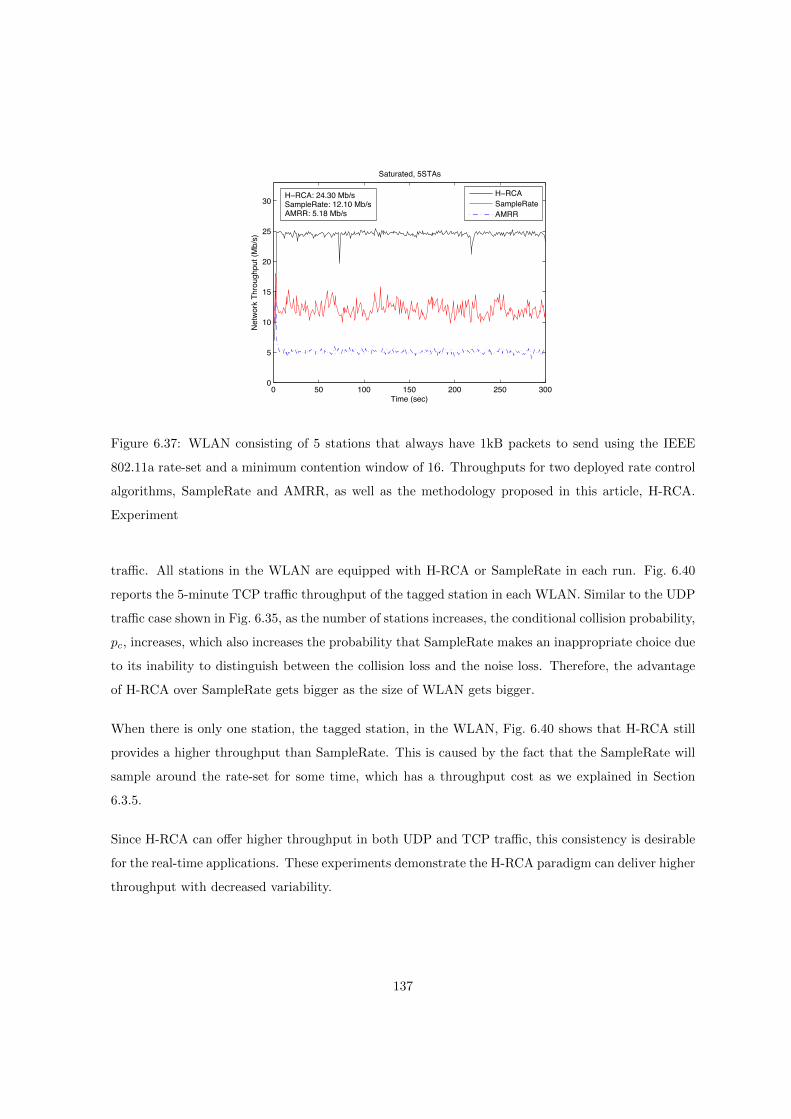
0 50 100 150 200 250 3000

5

10

15

20

25

30

Time (sec)

Net

wor

k Th

roug

hput

(Mb/

s)

Saturated, 5STAs


H−RCA: 24.30 Mb/sSampleRate: 12.10 Mb/sAMRR: 5.18 Mb/s

Figure 6.37: WLAN consisting of 5 stations that always have 1kB packets to send using the IEEE

802.11a rate-set and a minimum contention window of 16. Throughputs for two deployed rate control

algorithms, SampleRate and AMRR, as well as the methodology proposed in this article, H-RCA.

Experiment

traffic. All stations in the WLAN are equipped with H-RCA or SampleRate in each run. Fig. 6.40

reports the 5-minute TCP traffic throughput of the tagged station in each WLAN. Similar to the UDP

traffic case shown in Fig. 6.35, as the number of stations increases, the conditional collision probability,

pc, increases, which also increases the probability that SampleRate makes an inappropriate choice due

to its inability to distinguish between the collision loss and the noise loss. Therefore, the advantage

of H-RCA over SampleRate gets bigger as the size of WLAN gets bigger.

When there is only one station, the tagged station, in the WLAN, Fig. 6.40 shows that H-RCA still

provides a higher throughput than SampleRate. This is caused by the fact that the SampleRate will

sample around the rate-set for some time, which has a throughput cost as we explained in Section

6.3.5.

Since H-RCA can offer higher throughput in both UDP and TCP traffic, this consistency is desirable

for the real-time applications. These experiments demonstrate the H-RCA paradigm can deliver higher

throughput with decreased variability.

137

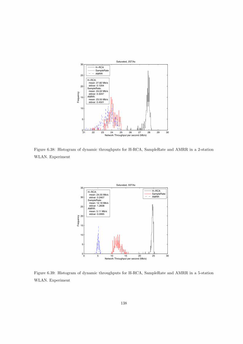
21 22 23 24 25 26 27 28 29 300

5

10

15

20

25

30

Network Throughput per second (Mb/s)

Freq

uenc

y

Saturated, 2STAs


H−RCA: mean: 27.82 Mb/s stdvar: 0.1204SampleRate: mean: 24.02 Mb/s stdvar: 0.3247AMRR: mean: 23.55 Mb/s stdvar: 0.4501

Figure 6.38: Histogram of dynamic throughputs for H-RCA, SampleRate and AMRR in a 2-station

WLAN. Experiment

0 5 10 15 20 25 300

5

10

15

20

25

30

35

Network Throughput per second (Mb/s)

Freq

uenc

y

Saturated, 5STAs


H−RCA: mean: 24.55 Mb/s stdvar: 0.2407SampleRate: mean: 12.16 Mb/s stdvar: 1.2838AMRR: mean: 5.11 Mb/s stdvar: 0.0995

Figure 6.39: Histogram of dynamic throughputs for H-RCA, SampleRate and AMRR in a 5-station

WLAN. Experiment

138

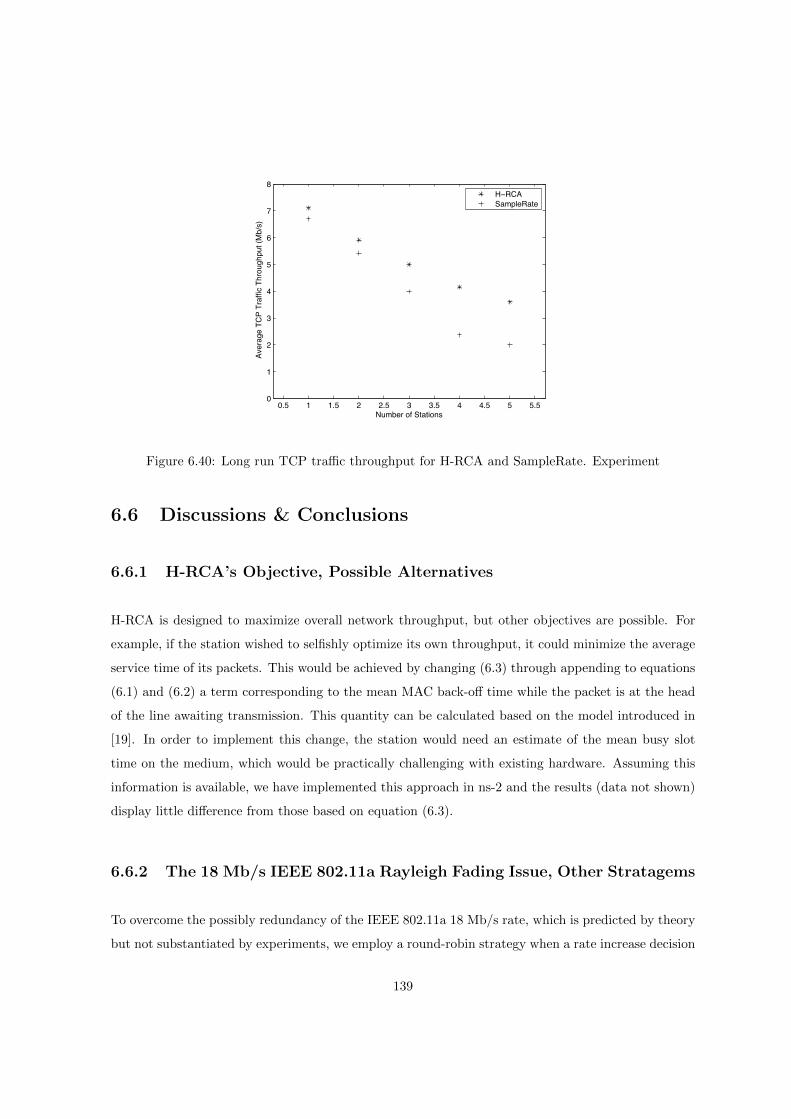
0.5 1 1.5 2 2.5 3 3.5 4 4.5 5 5.50

1

2

3

4

5

6

7

8

Number of Stations

Aver

age

TCP

Traf

fic T

hrou

ghpu

t (M

b/s)

H RCASampleRate

Figure 6.40: Long run TCP traffic throughput for H-RCA and SampleRate. Experiment

6.6 Discussions & Conclusions

6.6.1 H-RCA’s Objective, Possible Alternatives

H-RCA is designed to maximize overall network throughput, but other objectives are possible. For

example, if the station wished to selfishly optimize its own throughput, it could minimize the average

service time of its packets. This would be achieved by changing (6.3) through appending to equations

(6.1) and (6.2) a term corresponding to the mean MAC back-off time while the packet is at the head

of the line awaiting transmission. This quantity can be calculated based on the model introduced in

[19]. In order to implement this change, the station would need an estimate of the mean busy slot

time on the medium, which would be practically challenging with existing hardware. Assuming this

information is available, we have implemented this approach in ns-2 and the results (data not shown)

display little difference from those based on equation (6.3).

6.6.2 The 18 Mb/s IEEE 802.11a Rayleigh Fading Issue, Other Stratagems

To overcome the possibly redundancy of the IEEE 802.11a 18 Mb/s rate, which is predicted by theory

but not substantiated by experiments, we employ a round-robin strategy when a rate increase decision

139

occurs from 12 Mb/s. Many other schemes could be proposed, including adaptive schemes, but the

simplest one appears to function adequately in our tests. For example, we implemented a weighted

scheme in which, on a rate increase decision the 18 Mb/s and 24 Mb/s rates were selected with

frequencies related to the potential lost bandwidth if pn = 1. In all tests, the results from this scheme

were directly comparable to the round-robin methodology.

6.6.3 Non-saturated Stations

We have focused on stations that have back-to-back packets to send so that they can be packaged in

pairs in TXOP bursts. This is reasonable as it is when stations have a lot of traffic to send that efficient

usage is of particular importance. If stations are extremely lightly loaded there are two alternative

stratagems. If stations have large packets, the MAC can split them into two fragments the second of

which is not subject to collisions. If stations have small packets, this is unnecessary and they can be

sent individually as the dominant component of the transmission delay comes from fixed overheads in

that case.

6.6.4 Hidden Nodes

Rate-control in itself is not a solution to the problem of hidden nodes, but can be used to mitigate

their impact. The scheme we employ to separate collision and noise based losses can be extended

using standard IEEE 802.11e functionality to distinguish between hidden nodes based losses too [56].

H-RCA can be readily modified to make use of this information in order to keep transmission rates

high when noise is low, but hidden nodes are present. This is a only partial solution as completely

mitigating the effect of hidden nodes is within the remit of power and channel selection.

6.6.5 Summary

We have presented H-RCA, an adaptive collision-aware wireless rate control methodology. As H-

RCA does not require specific hardware support nor any change in IEEE 802.11 standard, we have

implemented it on commodity hardware.

Due to its TXOP technique to distinguish the collision loss, H-RCA adapts appropriately to collision

140

induced losses. Its rate decrease decision making process employs Bayesian analysis to ensure reason-

able outcomes. Its increase-rate decision frequency is chosen in a way that guarantees near optimal

performance in an unchanging environment.

As well as offering increased mean throughput over existing algorithms, experiments demonstrate

that H-RCA also offers decreased variance in throughputs. This consistency is desirable for real-time

applications that rely on high throughput and low jitter. It is also desirable for non-real-time traffic

as the performance of TCP is dependent upon stable round-trip time statistics.

141

Bibliography

[1] Minstrel rate adaptation algorithm. http://madwifi-project.org/browser/madwifi/trunk/

ath_rate/minstrel, Jan 2010.

[2] Multi-generator. http://cs.itd.nrl.navy.mil/work/mgen/, May 2010.

[3] Multiband Atheros driver for WiFi (MADWiFi). http://sourceforge.net/projects/

madwifi/, Jan 2010.

[4] Onoe rate adaptation algorithm. http://madwifi-project.org/browser/madwifi/trunk/

ath_rate/onoe, Jan 2010.

[5] Soekris engineering. http://www.soekris.com/, Jan 2010.

[6] Tcpdump. http://www.tcpdump.org/, May 2010.

[7] P.A.K. Acharya, A. Sharma, E.M. Belding, K.C. Almeroth, and D. Papagiannaki. Congestion-

aware rate adaptation in wireless networks: a measurement-driven approach. In IEEE Com-

munications Society Conference on Sensor, Mesh and Ad Hoc Communications and Networks,

2008.

[8] G.S. Ahn, A.T. Campell, A. Veres, and L.H. Sun. Supporting service differentiation for real-

time and best-effort traffic in stateless wireless ad hoc networks SWAN. IEEE Transactions on

Mobile Computing, 1(3):192–207, 2002.

[9] A. Akella, G. Judd, S. Seshan, and P. Steenkiste. Self-management in chaotic wireless deploy-

ments. In 11th International Conference on Mobile Computing and Networking, 2005.

[10] A.A. Ali and K. Alkhudairi. BER for M-QAM with space-time transmit diversity in Nakagami

and Rician fading channelss. Technical report, King Saud University, 2009.

142

[11] S. Asmussen. Applied Probability and Queues, volume 51. Springer-Verlag, New York, 2003.

[12] Y. Barowski and S. Biaz. The performance analysis of IEEE 802.11 under unsaturated traffic

conditions. Technical Report CSSE0-4-09, Auburn University, 2004.

[13] Y. Barowski, S. Biaz, and P. Agrawal. Towards the performance analysis of IEEE 802.11 in

multi-hop ad-hoc networks. In Proceedings of IEEE Wireless Communications and Networking

Conference, 2005.

[14] C. Barrett, M.V. Marathe, D.C. Engelhart, and A. Sivasubramaniam. Analysing the short-term

fairness of IEEE 802.11 in wireless multi-hop radio networks. In Proceedings of IEEE/ACM

Modelling, Analysis and Simulation of Computer and Telecommunication Systems, 2002.

[15] P. Barsocchi, G. Oligeri, and F. Potortia. Validation for 802.11b Wireless Channel Measure-

ments. Technical report, Istituto di Scienza e Tecnologie dell’Informazione ‘Ales sandro Faedo’,

2006.

[16] G. Berger-Sabbatel, A. Duda, M. Heusse, and F. Rousseau. Short-term fairness of 802.11

networks with several hosts. In Proceedings of International Conference on Mobile and Wireless

Communications Networks, October 2004.

[17] D.P. Bertsekas and R.G. Gallager. Data Networks, 2nd Ed. Prentice-Hall, 1991.

[18] G. Bianchi. IEEE 802.11 - saturated throughput analysis. IEEE Communications Letters,

12(2):318–320, December 1998.

[19] G. Bianchi. Performance analysis of IEEE 802.11 distributed coordination function. IEEE

Journal on Selected Areas in Communications, 18(3):535–547, March 2000.

[20] G. Bianchi, A. Di Stefano, C. Gianconia, and L. Scalia. Experimental assessment of the backoff

behavior of commercial IEEE 802.11b network. In Proceedings of IEEE International Conference

on Computer Communications, 2007.

[21] S. Biaz and Nitin H. Vaidya. Discriminating congestion losses from wireless losses using inter-

arrival times at the receiver. In IEEE Application-Specific Systems and Software Engineering

Technology Symposium, 1999.

[22] J. Bicket. Bit-Rate Selection in Wireless Networks. Master’s thesis, Massachusetts Institute of

Technology, 2005.

143

[23] P. Billingsley. Convergence of Probability Measures. Wiley Series in Probability and Statistics:

Probability and Statistics. John Wiley & Sons Inc., New York, second edition, 1999. A Wiley-

Interscience Publication.

[24] S. Biswas and R. Morris. Opportunistic routing in multi-hop wireless networks. In Proceedings

of ACM Special Interest Group on Data Communication, pages 133–144, 2005.

[25] J.R. Blum, J. Kiefer, and M. Rosenblatt. Distribution free tests of independence based on the

sample distribution function. Annals of Mathematical Statistics, 32:485–498, 1961.

[26] L. Bononi, M. Conti, and E. Gregori. Runtime optimization of IEEE 802.11 wireless LANs

performance. IEEE Transactions on Parallel and Distributed Systems, 15(1):66–80, 2004.

[27] C. Bordenave, S. Foss, and V. Shneer. A random multiple access protocol with spatial interac-

tions. Journal of Applied Probability, 46:844–865, 2009.

[28] C. Bordenave, D. McDonald, and A. Proutiere. A particle system in interaction with a rapidly

varying environment: mean field limits and applications. Networks and Heterogeneous Media,

5(1), 2010.

[29] C. Bordenave, A. Proutiere, and D. McDonald. Random multi-access algorithms, a mean field

analysis. In Proceedings of Allerton Communication, Control and Computing, 2005.

[30] R. Bruno, M. Conti, and E. Gregori. IEEE 802.11 optimal performances: RTS/CTS mechanism

VS . basic access. In IEEE International Symposium on Personal, Indoor and Mobile Radio

Communications, 2002.

[31] F. Cali, M. Conti, and E. Gregori. Dynamic tuning of the IEEE 802.11 protocol to achieve a

theoretical throughput limit. IEEE/ACM Transactions on Networking, 8(6):785–799, 2000.

[32] F. Cali, M. Conti, and E. Gregori. IEEE 802.11 protocol: design and performance evalua-

tion of an adaptive backoff mechanism. IEEE Journal on Selected Areas in Communications,

18(9):1774–1786, 2000.

[33] G.R. Cantieni, Q. Ni, C. Barakat, and T. Turletti. Performance analysis under finite load

and improvements for multirate 802.11. Elsivier Computer Communications, 28(10):1095–1109,

2005.

[34] X. Chen, H. Zhai, X. Tian, and Y. Fang. Supporting QoS in IEEE 802.11e wireless LANs. IEEE

Transactions on Wireless Communications, 5(8):2217–2227, August 2006.

144

[35] J. Choi, J. Na, Y.S. Lim, K. Park, and C.K. Kim. Adaptive optimization of rate adaptation

algorithms in multi-rate wlans. In IEEE International Conference on Network Protocols, 2007.

[36] J. Choi, J. Na, Y.S. Lim, K. Park, and C.K. Kim. Cross-layer analysis of rate adaptation, DCF

and TCP in multi-rate wlans. In IEEE International Conference on Computer Communications,

2007.

[37] J. Choi, J. Na, Y.S. Lim, K. Park, and C.K. Kim. Collision-aware design of rate adaptation for

multi-rate 802.11 wlans. IEEE Journal on Selected Areas in Communications, 26(8):1366–1375,

2008.

[38] S. Choudhury and J. D. Gibson. Payload Length and Rate Adaptation for Throughput Opti-

mization in Wireless LANs. In Vehicular Technology Conference, 2006.

[39] P. Clifford, K. Duffy, J. Foy, D.J. Leith, and D. Malone. Modeling 802.11e for data traffic pa-

rameter design. In Proceedings of International Conference on Resource Allocation, Cooperation

and Competition in Wireless Networks, 2006.

[40] W. J. Conover. A Kolmogorov goodness-of-fit test for discontinuous distributions. Journal of

the American Statistical Association, 67:591–596, 1972.

[41] O. Dousse, P. Thiran, and M. Durvy. On the fairness of large CSMA networks. IEEE Journal

on Selected Areas in Communications, 27(7):1093–1104, 2009.

[42] R. Draves, J. Padhye, and B. Zill. Routing in multi-radio, multi-hop wireless mesh networks.

In Proceedings ACM Mobile Communications, pages 114–128, 2004.

[43] K. Duffy and A. J. Ganesh. Modeling the impact of buffering on 802.11. IEEE Communications

Letters, 11(2):219–221, 2007.

[44] K. Duffy, D. J. Leith, T. Li, and D. Malone. Modeling 802.11 mesh networks. IEEE Commu-

nications Letters, 10(8):635–637, 2006.

[45] K. Duffy, D. Malone, and D.J. Leith. Modeling the 802.11 distributed coordination function in

non-saturated conditions. IEEE Communications Letters, 9(8):715–717, 2005.

[46] Rick Durret. Essentials of Stochastic Processes. Springer, 1999.

[47] P. E. Engelstad and O. N. Østerbø. Non-saturation and saturation analysis of IEEE 802.11e

EDCA with starvation prediction. In Proceedings of ACM International Conference on Modeling,

Analysis and Simulation of Wireless and Mobile Systems, 2005.

145

[48] M. Ergen and P. Varaiya. Throughput analysis and admission control in IEEE 802.11a. ACM-

Kluwer Mobile Networks and Applications, 10(5):705–716, 2005.

[49] L.M. Feeney. An energy comsumption model for performance analysis of routing protocols for

mobile Ad Hoc networks. Mobile Networks and Applications, 6(3):239 – 249, June 2001.

[50] C.H. Foh and M. Zukerman. Performance evaluation of IEEE 802.11. In 53rd IEEE Vehicular

Technology Conference, volume 2, pages 841–845, 2001.

[51] C.H. Foh and M. Zukerman. Performance analysis of the IEEE 802.11 MAC protocol. In

Proceedings of the European Wireless conference, Florence, Italy, pages 184–190, 2002.

[52] Y. Gao, D. Chiu, and J. Lui. The fundamental role of hop distance in IEEE 802.11 multi-hop ad

hoc networks. In Proceedings of International Conference on Network Protocols, pages 75–84,

2005.

[53] E. Garcia, R. Vidal, and J. Paradells. New algorithm for distributed frequency assignments in

IEEE 802.11 wireless networks. In 11th European Wireless Conference, 2005.

[54] Matthew S. Gast. 802.11 Wireless networks. O’Reilly, 2002.

[55] D. Giustiniano, G. Bianchi, L. Scalia, and I. Tinnirello. An explanation for unexpected 802.11

outdoor link-level measurement results. In Proceedings of IEEE International Conference on

Computer Communications, 2008.

[56] D. Giustiniano, D. Malone, D. J. Leith, and K. Papagiannaki. Measuring transmission oppor-

tunities in 802.11 links. IEEE/ACM Transactions on Networking, 18(5):1516–1529, 2010.

[57] A. Goldsmith. Wireless Communications. CUP, 2005.

[58] J. Hagenauer. Viterbi decoding of convolutional codes for fading- and burst-channels. In Pro-

ceedings of the 1980 Zurich seminar on digital communications, 1980.

[59] G. Hauksson and M. Alanyali. Wireless medium access via adaptive backoff: delay and loss

minimization. In Proceedings of IEEE International Conference on Computer Communications,

2008.

[60] W. Hoeffding. A non-parametric test of independence. Annals of Mathematical Statistics,

19:546–557, 1948.

146

[61] W. Hoeffding. Probability inequalities for sums of bounded random variables. Journal of the

American Statistical Association, 58:13–30, 1963.

[62] G. Holland, N. Vaidya, and P. Bahl. A rate-adaptive MAC protocol for multi-hop wireless

networks. In ACM Mobile Systems Conference, 2001.

[63] K.D. Huang and K.R. Duffy. On a buffering hypothesis in 802.11 analytic models. IEEE

Communications Letters, 13(5):312–314, 2009.

[64] K.D. Huang, K.R. Duffy, and D. Malone. On the validity of IEEE 802.11 MAC modeling

hypotheses. IEEE/ACM Transactions on Networking, 18(6):1935–1948, 2010.

[65] K.D. Huang, K.R. Duffy, and D. Malone. H-RCA: collision-aware rate control algorithm. Tech-

nical report, Hamilton Institute, 2011.

[66] K.D. Huang, K.R. Duffy, D. Malone, and D.J. Leith. Investigating the validity of IEEE 802.11

MAC modeling hypotheses. In Proceedings of IEEE International Symposium on Personal,

Indoor and Mobile Radio Communications, 2008.

[67] K.D. Huang, D. Malone, and K.R. Duffy. The 802.11g 11mb/s rate is more robust than 6mb/s.

IEEE Transactions on Wireless Communications, 10(4):1015–1020, 2010.

[68] J. Hui and M. Devetsikiotis. A unified model for the performance analysis of IEEE 802.11e

EDCA. IEEE Transactions on Communications, 53(9):1498–1510, 2005.

[69] Glover Ian and M. Grant Peter. Digital Communications. Pearson Education Limited, 2004.

[70] IEEE. Wirless LAN Medium Access Control (MAC) and Physical Layer (PHY) Specifications,

IEEE std 802.11-1997 edition, 1997.

[71] IEEE. Wirless LAN Medium Access Control (MAC) and Physical Layer (PHY) Specifications:

Medium Access Control (MAC) enhancements for Quality of Service (QoS), IEEE std 802.11e

edition, 2005.

[72] IEEE Std 802.15.2. Coexistence of wireless personal area networks with other wireless devices

operating inunlicensed frequency bands, Aug. 2003.

[73] Information Sciences Institute. The Network Simulator - ns-2. The University of Southern

California, July 2006.

147

[74] G. Judd, X. Wang, and P. Steenkiste. Efficient channel-aware rate adaptation in dynamic

environments. In ACM International Conference on Mobile Systems, Applications, and Services,

2008.

[75] A. Kamerman and L. Monteban. Wavelan II: a high-performance wireless LAN for the unlicensed

band. Bell Labs Technical Journal, 2(3):118–133, 1997.

[76] T. Khattab, M.T. El-Hadidi, and H.M. Mourad. Analysis of wireless CSMA/CA network using

single station superposition (SSS). International Journal of Electronics and Communications,

56(2):73–83, 2002.

[77] H. Kim and J. C. Hou. Improving protocol capacity with model-based frame scheduling in

IEEE 802.11-operated wlans. In Proceedings of the 9th annual international conference on

Mobile computing and networking, pages 190 – 204, 2003.

[78] J. Kim, S. Kim, S. Choi, and D. Qiao. CARA: collision-aware rate adaptaion for 802.11 wireless

networks. In IEEE International Conference on Computer Communications, 2006.

[79] C. E. Koksal, H. Kassab, and H. Balakrishnan. An analysis of short-term fairness in wireless

media access protocols. In Proceedings of ACM SIGMETRICS, June 2000.

[80] Z. Kong, D.H.K. Tsang, B. Bensaou, and D. Gao. Performance analysis of IEEE 802.11e

contention-based channel access. IEEE Journal on Selected Areas in Communications,

22(10):2095–2106, December 2004.

[81] A. Kumar. Analysis and optimisation of IEEE 802.11 wireless local area networks. In Proceedings

of Modeling and Optimization in Mobile, Ad Hoc, and Wireless Networks, April 2005.

[82] A. Kumar, E. Altman, D. Miorandi, and M. Goyal. New insights from a fixed point analysis

of single cell IEEE 802.11 WLANs. IEEE/ACM Transactions on Networking, 15(3):588–601,

2007.

[83] M. Lacage, M. Manshaei, and T. Turletti. IEEE 802.11 rate adaptation: a practical approach.

In ACM International Conference on Modeling, Analysis and Simulation of Wireless and Mobile

Systems, 2004.

[84] S. Lee, S. Banerjee, and B. Bhattacharjee. The case for a multi-hop wireless local area network.

In Proceedings of IEEE International Conference on Computer Communications, pages 894–905,

2004.

148

[85] D. Leskaroski and W.B. Michael. Frequency planning and adjacent channel interference in a

DSSS wireless local area network (WLAN). In Wireless Personal Communications: Bluetooth

Tutorial and Other Technologies, pages 169 – 180. Kluwer Academic Publishers, 2001.

[86] B. Li and R. Battiti. Supporting service differentiation with enhancements of the IEEE 802.11

MAC protocol: models and analysis. Technical Report DIT-03-024, University of Trento, May

2003.

[87] William Lindsey. Error probabilities for rician fading multichannel reception of binary and n-ary

signals. IEEE Transactions on Information Theory, 10:339–350, 1964.

[88] C. Liu and F. Lee. Spectrum modelling of ofdm signals for wlan. Electronics Letters, 40:1431 –

1432, October 2004.

[89] G. M. Ljung and G.E.P. Box. On a measure of a lack of fit in time series models. Biometrika,

65:297–303, 1978.

[90] S. Lv, X. Wang, X. Zhou, and C. Liu. Self-learning rate adaptation in multi-rate 802.11 networks.

In Wireless Communications, Networking and Mobile Computing, 2007.

[91] O. Dousse M. Durvy and P. Thiran. Self-organization properties of CSMA/CA systems and their

consequences on fairness. IEEE Transactions on Information Theory, 55(3):931–943, 2009.

[92] D. Malone, I. Dangerfield, and D.J. Leith. Verification of common 802.11 mac model assump-

tions. In Proceedings of Passive and Active Measurement Workshop, LNCS 4427, pages 63–72,

2007.

[93] D. Malone, K. Duffy, and D.J. Leith. Modelling the 802.11 DCF under heterogeneous finite load.

In Proceedings of International Conference on Resource Allocation, Cooperation and Competition

in Wireless Networks, 2005.

[94] D. Malone, K.R. Duffy, and D.J. Leith. Modeling the 802.11 distributed coordination function in

non-saturated heterogeneous conditions. IEEE/ACM Transactions on Networking, 15(1):159–

172, 2007.

[95] H.B. Mann and A. Wald. On the choice of the number of class intervals in the application of

the chi square test. Annals of Mathematical Statistics, 13:306–317, 1942.

[96] A.P. Markopoulou, F.A. Tobagi, and M.J. Karam. Assessing the quality of voice communications

over internet backbones. IEEE/ACM Transactions on Networking, 11(5):747–760, October 2003.

149

[97] J Mikulka and S Hanus. Cck and barker coding implementation in IEEE 802.11b standard. In

Radioelektronika, 2007.

[98] A.M. Mood. The distribution theory of runs. Annals of Mathematical Statistics, 11:367–392,

1940.

[99] S. Narayanan, P. Liu, and S. Panwar. On the advantages of multi-hop extensions to the IEEE

802.11 infrastructure model. In Proceedings of IEEE Wireless Communications and Networking

Conference, pages 132–138, 2005.

[100] Q. Ni, T. Li, T. Turletti, and Y. Xiao. Saturation throughput analysis of error-prone 802.11

wireless networks. Wiley Journal of Wireless Communications and Mobile Computing, 5(8):945–

957, 2005.

[101] C.G. Park, D.H. Han, and S. J. Ahn. Performance analysis of MAC layer protocols in the IEEE

802.11 wireless LAN. Telecommunication Systems, 33(1–3):233–253, 2006.

[102] A.N. Pettitt and M.A. Stephens. The Kolmogorov-Smirnov goodness-of-fit statistic with discrete

and grouped data. Metrika, 19(2):205–210, 1977.

[103] M.B. Pursley and T.C. Royster IV. Properties and performance of the IEEE 802.11b

complementary-code-key signal sets. IEEE Transactions on Communications, 57(2), February

2005.

[104] M.B. Pursley and D. J. Taipale. Error probabilities for spreadspectrum packet radio with

convolutional codes and viterbi decoding. IEEE Transactions on Communications, 35(1):1–12,

1987.

[105] Byron W. Putman. 802.11 WLAN Hands-On Analysis. AuthorHouse, 2005.

[106] D. Qiao, S. Choi, and K. G. Shin. Goodput analysis and link adaptation for IEEE 802.11a

wireless LANs. IEEE Transactions on Mobile Computing, 1(4):278–292, 2002.

[107] D. Raguin, M. Kubisch, H. Karl, and A. Wolisz. Queue-driven cut-through medium access in

wireless ad hoc networks. In Proceedings of IEEE Wireless Communications and Networking

Conference, pages 1909 – 1914, 2004.

[108] S. Rahman. Throughput analysis of IEEE 802.11 Distributed Coordination Function in presence

of hidden stations. Technical report, Stanford University, 2003.

150

[109] A. Raniwala and T. Chiueh. Architecture and algorithms for an IEEE 802.11-based multi-

channel wireless mesh network. In Proceedings of IEEE International Conference on Computer

Communications, pages 2223–2234, 2005.

[110] S. Rayanchu, A. Mishra, D. Agrawal, S. Saha, and S. Banerjee. Diagnosing wireless packet

losses in 802.11: separating collision from weak signal. In IEEE International Conference on

Computer Communications, 2008.

[111] J.W. Robinson and T. S. Randhawa. Saturation throughput analysis of IEEE 802.11e en-

hanced distributed coordination function. IEEE Journal on Selected Areas in Communications,

22(5):917–928, June 2004.

[112] B. Sadeghi, V. Kanodia, A. Sabharwal, and E. Knightly. Opportunistic media access for multi-

rate ad hoc networks. In ACM Mobile Systems Conference, 2002.

[113] F.A. Shabdiz and S. Subramaniam. Performance analysis of the IEEE 802.11 MAC protocol.

In Proceedings of Modeling and Optimization in Mobile, Ad Hoc, and Wireless Networks, 2003.

[114] G. Sharma, A. Ganesh, and P. Key. Performance analysis of contention based medium access

control protocols. IEEE Transactions on Information Theory, 55(4):1665–1682, 2009.

[115] G. Sharma, A.J. Ganesh, and P. Key. Performance analysis of contention based medium access

control protocols. In Proceedings of IEEE International Conference on Computer Communica-

tions, 2006.

[116] M.K. Simon and M.S. Alouini. A unified approach to the performance analysis of digital com-

munication over generalized fading cahnnels. Proceedings of the IEEE, 86(9):1860–1877, 1998.

[117] M.K. Simon and M.S. Alouini. Digital Communication over Fading Channels. Wiley-IEEE

Press, 2005.

[118] H.J. Skaug and D. Tjøstheim. A nonparametric test of serial independence based on the empirical

distribution function. Biometrika, 80(3):591–602, 1993.

[119] William Stallings. Computer Networking with Internet Protocols and Technology. Publishing

House of Electronics Industry, 2006.

[120] Std. 802.11a. IEEE: Supplement to standard for information technology - telecommunications

and information exchange between systems - local and metropolitan area networks -specific re-

quirements. Part 11: wireless LAN medium access control (MAC) and physical layer (PHY)

specifications: High speed physical layer in the 5 GHz band, September 1999.

151

[121] Y. Sun, X. Gao, E. Belding-Royer, and J. Kempf. Model-based resource prediction for multi-hop

wireless networks. In Proceedings of IEEE Mobile Ad-hoc and sensor Systems, pages 114–123,

2004.

[122] O. Tickoo and B. Sikdar. A queueing model for finite load IEEE 802.11 random access. In IEEE

International Conference on Computer Communications, volume 1, pages 175 – 179, June 2004.

[123] O. Tickoo and B. Sikdar. Modeling queueing and channel access delay in unsaturated IEEE

802.11 random access MAC based wireless networks. IEEE/ACM Transactions on Networking,

16(4):878–891, August 2008.

[124] H.C. Tijms. A First Course in Stochastic Models. John Wiley & Sons Inc., 2003.

[125] I. Tinnirello, D. Giustiniano, L. Scalia, and G. Bianchi. On the side-effects of proprietary

solutions for fading and interference mitigation in IEEE 802.11b/g outdoor links. Elsevier

Computer Network Journal, 2009.

[126] D. Vassis, G. Kormentzas, A. Rouskas, and I. Maglogiannis. The IEEE 802.11g standard for

high data rate wlans. IEEE Network, 19(3):21 – 26, 2005.

[127] Eduard Garcia Villegas, Elena Lopez Aguilera, Rafael Vidal, and Josep Paradells. Effect of

adjacent-channel interference in IEEE 802.11 WLANs. In International ICST Conference on

Cognitive Radio Oriented Wireless Networks and Communications, 2007.

[128] Andrew J. Viterbi. Convolutional codes and their performance in communication systems. IEEE

Transactions on Communications Technology, COM-19(5):751 – 772, 1971.

[129] M. Vutukuru, H. Balakrishnan, and K. Jamieson. Cross-layer wireless bit rate adaptation. In

ACM Special Interest Group on Data Communication, 2009.

[130] D. O. Wackerly, W. Mendenhall, and R. L. Scheaffer. Mathematical Statistics with Applications,

volume 6. Duxbury Press, CA, 2001.

[131] A. Wald and J. Wolfowitz. On a test whether two samples are from the same population. Annals

of Mathematical Statistics, 11(2):147–162, 1940.

[132] Y. Wang and J.J. Garcia-Luna-Aceves. Collision avoidance in multi-hop ad hoc networks. In

Proceedings of IEEE Modeling Analysis and Simulation of Computer and Telecommunication

Systems, pages 640–649, 2002.

152

[133] L. F. White, M. Bonetti, and M. Pagano. The choice of the number of bins for the M statistic.

Computational Statistics and Data Analysis, 53(10):3640–3649, 2009.

[134] S. Wietholter and C. Hoene. Design and verification of an IEEE 802.11e EDCF simulation model

in ns-2.26. Technical Report TKN-03-019, Technische Universitat Berlin, November 2003.

[135] David Williams. Weighing the Odds. A Course in Probability and Statistics. Cambridge Uni-

versity Press, 2001.

[136] S. Wong, H. Yang, S. Lu, and V. Bharghavan. Robust rate adaptation for 802.11 wireless

networks. In ACM Mobile Systems Conference, 2008.

[137] K. Xu, M. Gerla, and S. Bae. How effective is the IEEE 802.11 RTS/CTS handshake in ad hoc

networks. In Global Telecommunications Conference, volume 1, pages 72 – 76, 2002.

[138] X. Yang and N. Vaidya. On physical carrier sense in wireless ad hoc networks. In IEEE

International Conference on Computer Communications, 2005.

[139] F. Ye, S. Yi, and B. Sikdar. Improving spatial reuse of IEEE 802.11 based ad hoc networks. In

Global Communications Conference, pages 1013 – 1017, 2003.

[140] A.N. Zaki and M.T. El-Hadidi. Throughput analysis of IEEE 802.11 DCF under finite load

traffic. In First International Symposium on Control, Communications and Signal Processing,

pages 535–538, 2004.

[141] A. Zanella and F. De Pellegrini. Statistical characterization of the service time in saturated

IEEE 802.11 networks. IEEE Communications Letters, 9(3):225–227, 2005.

[142] Hongqiang Zhai, Younggoo Kwon, and Yuguang Fang. Performance analysis of IEEE 802.11

MAC protocols in wireless LANs. Wireless Communications and Mobile Computing, 4(8):917–

931, 2004.

[143] J. Zhang, K. Tan, J. Zhao, H. Wu, and Y. Zhang. A practical SNR-guided rate adaptation. In

IEEE International Conference on Computer Communications, 2008.

[144] Eustathia Ziouva and Theodore Antonakopoulos. CSMA/CA performance under high traffic

conditions: throughput and delay analysis. Computer Communications, 25(3):313–321, 2002.

153

Appendix A

A brief overview of 802.11’s BEB

algorithm

On detecting the wireless medium to be idle for a period of Distributed Inter-Frame Space (DIFS), each

station initializes a counter to a random number selected uniformly in the range {0, 1, . . . ,W − 1},

where W is the contention window and equals to the minimal contention window Wmin. Time is

slotted and this counter is decremented once during each slot that the medium is observed idle. The

count-down halts when the medium becomes busy and resumes after the medium is idle again for a

period DIFS. Once the counter reaches zero the station attempts transmission and if a collision does

not occur it can transmit for a duration up to a maximum period TXOP (defined to be one packet

except in the quality of service MAC extension IEEE 802.11e). If two or more stations attempt to

transmit simultaneously, a collision occurs. Colliding stations double their contention window W ,

up to a maximum value 2mWmin, selects a new back-off counter uniformly and the process repeats.

If a packet experiences more collisions than the retry limit, M , the packet is discarded. After the

successful transmission of a packet or after a packet discard, W is reset to its minimal value Wmin

and a new count-down starts regardless of the presence of a packet at the MAC. If a packet arrives

at the MAC after the count-down is completed, the station senses the medium. If the medium is

idle, the station attempts transmission immediately; if it is busy, another back-off counter is chosen

from the minimum interval. This bandwidth saving feature is called post-back-off. The revised IEEE

802.11e MAC enables the values of DIFS (called the Arbitration Inter-Frame Spacing, AIFS, in IEEE

154

802.11e), Wmin and TXOP to be set on a per-class basis for each station. That is, traffic is directed to

up to four different queues at each station, with each queue assigned different MAC parameter values.

155

Appendix B

Testing Goodness of Fit

To test the validity of a hypothesis is the question of ‘testing goodness of fit’. Given a sequence of

observations of independent and identically distributed random variables X1, . . . , Xn, we wish to test

the hypothesis that the {Xk} have common distribution F . For discrete-valued random variables

taking N distinct values, we use Pearson’s χ2-test (e.g. [130]). Assume a null hypothesis that X1 has

a distribution such that P (X1 = i) = f(~θ, i), where ~θ is a collection of M parameters estimated from

the data. For each possible outcome i define:

ni :=

n∑j=1

1(Xj=i) and X2 :=

N∑i=1

(ni − nf(~θ, i))2

nf(~θ, i).

For large sample sizes n, the test statistic X2 has a χ2 distribution with between N−1 and N−1−M

degrees of freedom. We use the latter, more stringent, test to determine the p-value P (χ2(N−1−M) ≥

X2).

For real-valued random variables and unbounded random variables with a discrete distribution we

evaluate the Kolmogorov-Smirnov statistic (e.g. [102][130]). We can use the former to determine a

test for goodness-of-fit, but exact critical levels are not possible to determine in the latter case [40].

Let

Fn(k) =1

n

n∑i=1

1(Xi≤k)

denote the empirical distribution given n observations. The L∞ distance supk |Fn(k) − F (k)| is the

greatest discrepancy between the two distributions. It is used in the the Kolmogorov-Smirnov test

156

based on the observation that if the null hypothesis that {Xk} are identically distributed were true,

then Dn := supk |Fn(k)− F (k)| is of order n−1/2 and, in particular, supk |Fn(k)− F (k)| → 0. If F is

continuous, we also have the following weak convergence result

√nDn ⇒ sup

t|B(F (t))|,

where B(t) is a Brownian bridge [23] from which a p-value can be determined.

157

Appendix C

Runs Test for Binary Valued

Random Variables

If {Xn} are binary valued random variables then the null hypothesis that the sequence is independent

and identically distributed can be efficiently tested using the Runs Test [98][130]. Given a sequence

of observations X1, . . . , Xn, a run is defined to be a maximal non-empty segment of the sequence

consisting of adjacent equal elements. Let R be the number of runs in X1, . . . , Xn and define

n0 =

n∑i=1

1{Xi=0}, µ =2n0(n− n0)

n+ 1, σ2 =

(µ− 1)(µ− 2)

n− 1.

Then, under the null hypothesis, Z = (R − µ)/√σ2 is asymptotically Normally distributed. Thus,

given the sequence of observations X1, . . . , Xn, one evaluates Z and the p-value for the null hypothesis

is min(P (N(0, 1) ≥ Z), P (N(0, 1) ≤ Z)), where N(0, 1) is a Normally distributed random variable.

158

Appendix D

Network Simulator 2

The Network Simulator 2 (ns-2) is a discrete event simulator targeted at networking research. The

ns-2 is built in C++ and provides a simulation interface through OTcl, an object-oriented dialect of

Tcl. The user describes a network topology by writing OTcl scripts, and then the main NS program

simulates that topology with specified parameters [73].

Ns-2 provides substantial support for the simulation of UDP, TCP, routing, and multicast proto-

cols over wired and wireless networks [73]. Since ns-2 gives an accurate simulation of traffic at the

MAC layer, it is widely used as a tool for comparison to predictions from analytical models (e.g.

[49][77][137][139]).

159

Appendix E

Experiment Apparatus

E.1 Atheros AR5215 802.11b/g

All systems described in this section are equipped with an Atheros AR5215 802.11b/g PCI card with

an external antenna. This card is run by a version of the MADWiFi [3] wireless driver modified to

allow packet transmissions at a chosen rate with RTS/CTS disabled and a specified queue size.

Care must be exercised when performing experiments with IEEE 802.11 devices. Bianchi et al. [20]

and Giustiniano et al. [55] report on extensive validation experiments which clearly demonstrate that

cards from many vendors fail to implement the protocol correctly. The precision of our experimental

apparatus was established using the methodology described in [20] with additional statistical tests.

For example, to check if the back-off counters are uniformly distributed, the sequence of transmission

times of a single saturated station with fixed packet sizes were recorded. The back-off counter values

were inferred from this sequence by evaluating the inter-transmission times less the time taken for

a packet transmission (DIFS+Payload+SIFS+Ack) and then dividing this quantity by the idle slot

length. When the contention window is 32 or 64, Fig. E.1 reports on a comparison of the protocol’s

back-off distribution with empirical distributions based on sample sizes of 8, 706, 941 and 7, 461, 686

respectively. With a null hypothesis that the distributions are uniform, Pearson’s χ2-test (described

in section B) gives p-values of 0.7437 and 0.2036 so that the null hypothesis would not be rejected.

160

There is one place where our 802.11 cards do not implement the standard correctly, but it does not

have an impact on our deductions. Both ACKTimeout and EIFS are shorter than suggested in the

standard. While this must be taken into account when, for example, predicting throughput, it has no

impact on the aspects of the MAC’s operation that are of interest to us.

E.2 Experiment Apparatus I

The experimental apparatus used for the results presented in Chapter 2 is set up in infrastructure

mode. It employs a PC acting as an Access Point (AP), another PC and 9 PC-based Soekris En-

gineering net4801 embedded Linux boxes [5] acting as client stations. For every transmitted packet,

the client PC records the transmitting timestamp (the time when it receives an ACK), the number

of retry attempts experienced and the absence or presence of another packet in station’s buffer, but

otherwise behaves as an ordinary client station. The transmission rate is fixed to 11 Mb/s. The 11

Mb/s rate is selected as in the absence of noise-based losses the MAC’s operation is rate independent

and more observations of transmission can be made at higher rates for an experiment of given real-

time duration. The channel on which experiments were conducted was confirmed to be noise free by

use of a spectrum analyzer and by conducting experiments with single transmitter-receiver pairs at

11 Mb/s.

All stations are equipped with a 100 Mbps wired Ethernet port that is solely used for control of

the test bed from a distinct PC. In the experiments, UDP traffic is generated by the Naval Research

Laboratory’s MGEN [2] in Poisson mode. All UDP packets have a 1000 byte payload and are generated

in client stations before being transmitted to the AP. At the AP, tcpdump [6] is used to record traffic

details.

Hoeffding’s concentration inequality (described in section 2.3.1) was used to determine how many

observations were necessary to ensure statistical confidence in estimated quantities. Consequently,

saturated and large buffer experiments were run for 2 hours while short buffer experiments were run

for 4 hours.

161

0 5 10 15 20 25 300

0.005

0.01

0.015

0.02

0.025

0.03

0.035

0.04

0.045

0.05

Back−off Counter Value

Prob

abilit

y

Contention Window Size = 32

ExperimentalTheoretical

!2 = 25.5260P−value = 0.7437

0 10 20 30 40 50 600

0.005

0.01

0.015

0.02

0.025

Back−off Counter Value

Prob

abilit

y

Contention Window Size = 64

ExperimentalTheoretical

!2 = 72.0458P−value = 0.2036

Figure E.1: Comparison of protocol’s uniform back-off distribution and empirical distribution for

contention windows of size 32 and 64 based on sample sizes of 8, 706, 941 and 7, 461, 686 respectively.

Pearson’s χ2 does not reject the hypothesis that the distributions are uniform. Experiment

162

E.3 Experiment Apparatus II

The experimental apparatus used for the results presented in Sections 6.1 and 6.5 employs a PC

acting as an Access Point (AP) and another 5 PCs acting as client stations. The WLAN is set up

in infrastructure mode. All systems are equipped with an Atheros AR5215 802.11 PCI card with

an external antenna. These cards do not suffer the serious difficulties reported in [20] and [55]. All

stations, including the AP, use a version of the MadWiFi wireless driver that supporting H-RCA,

SampleRate and AMRR, with RTS/CTS disabled. All stations are equipped with a 100 Mbps wired

Ethernet port that is solely used for control of the test bed from a distinct PC. In the experiments,

the UDP traffic is generated by the Naval Research Laboratory’s MGEN [2] in periodic mode, while

the TCP traffic is generated by using the linux command ‘scp’. All packets are generated in client

stations before being transmitted to the AP. Throughput information is collected at the AP using

tcpdump [6].

163

On Wireless Local Area Networks - Hamilton Institute · On Wireless Local Area Networks A...

Documents

Transcript of On Wireless Local Area Networks - Hamilton Institute · On Wireless Local Area Networks A...