
The Hartree-Fock-Bogoliubov Theory Bose-Einstein Condensates

—VUW—
Rigorous bounds
on
Transmission, Reflection,
and
Bogoliubov coefficients
by
Petarpa Boonserm
A thesis
submitted to Victoria University of Wellington
in fulfilment of the
requirements for the degree of
Doctor of Philosophy
in Mathematics.
Victoria University of Wellington
2009
arX
iv:0
907.
0045
v1 [
mat
h-ph
] 1
Jul
200
9


Abstract
This thesis describes the development of some basic mathematical tools of
wide relevance to mathematical physics. Transmission and reflection coeffi-
cients are associated with quantum tunneling phenomena, while Bogoliubov
coefficients are associated with the mathematically related problem of exci-
tations of a parametric oscillator. While many approximation techniques for
these quantities are known, very little is known about rigorous upper and
lower bounds.
In this thesis four separate problems relating to rigorous bounds on trans-
mission, reflection and Bogoliubov coefficients are considered, divided into
four separate themes:
• Bounding the Bogoliubov coefficients;
• Bounding the greybody factors for Schwarzschild black holes;
• Transformation probabilities and the Miller–Good transformation;
• Analytic bounds on transmission probabilities.
25 February 2009; LATEX-ed Wednesday, July 1, 2009; 12:39am
c© Petarpa Boonserm

ii

Acknowledgements
I would like to thank my supervisor, Professor Matt Visser for his guidance
and support. I am lucky to have such an active and hard working supervisor.
I really appreciate the effort he made for my thesis, making sure that things
got done properly and on time.
I am grateful to the School of Mathematics, Statistics, and Operations
Research for providing me with an office and all the facilities, and the Thai
Government Scholarship that provided me with funding.
I also would like to say thanks to my family who were also very supportive
and listened to me.
Finally, I would like to extend my gratitude to my friends, Adisorn Jun-
trasook, Nattakarn Kajohnwongsatit, Trin Sunathvanichkul, Jirayu Choti-
mongkol, Narit Pidokrajt, Anon Khamwon, Celine Cattoen, and Garoon
Pongsart for always being there to listen to me. I am not sure that this
thesis would have been finished without the support they showed.
i

ii
Preface
This thesis looks at a number of problems related to the derivation of rig-
orous bounds on transmission, reflection, and Bogoliubov coefficients: To
set the stage, we shall first briefly describe the general ideas underlying the
Schrodinger equation, and the concept of the WKB approximation for barrier
penetration probability. In addition, we shall present a discussion of some
general features of scattering theory in one space dimension. By considering
one-dimensional problems involving an incident beam of particles, we shall
derive an important connection between reflection and transmission ampli-
tudes. Furthermore, we shall collect several known analytic results, and show
how they relate to the general results presented in this thesis. We shall also
review and concisely describe the concept of quasinormal modes, and see how
most of the concepts introduced here are important tools for comparing the
bounds derived in the body of the thesis with known analytic results.
The technical heart of the thesis is this: We shall rewrite the second-order
Schrodinger equation as a set of two coupled first-order linear differential
equations (for which bounds can relatively easily be established). Systems of
differential equations of this type are often referred to as Shabat–Zakharov
systems or Zhakarov–Shabat systems. After this initial investigation, we
shall use this system of ODEs to derive our first bound, and then continue by
finding several slightly different ways of recasting the Schrodinger equation
as a 1st-order Shabat–Zakharov system, in this way deriving a number of
slightly different bounds.
Regarding the chapter “Bounding the Bogoliubov coefficients”, we have
iii

developed a distinct method for deriving general bounds on the Bogoliubov
coefficients, providing a largely independent derivation of the key results; a
seperate derivation that short-circuits much of the technical discussion.
Proceeding further along this branch of our investigation, we shall con-
sider the Regge–Wheeler equation for excitations of a scalar field defined on
a Schwarzschild spacetime, and adapt the general analysis of the previous
chapters to this specific case. We shall demonstrate that rigorous and ex-
plicit analytic bounds are indeed achievable. While these bounds may not
answer all the physical questions one might legitimately wish to ask, they
are definitely a solid step in the right direction.
We shall then use the Miller–Good transformation (which maps an initial
Schrodinger equation to a final Schrodinger equation for a different potential)
to significantly generalize the previous bound. Moreover, we shall then use
the Miller–Good transformation to generalize the bound to make it more
efficient.
Finally we shall consider analytic bounds on the transmission probabilities
obtained by comparing a simple “known” potential with a more complicated
“unknown” one. In this case we shall obtain yet another (distinct) Shabat–
Zakharov system and use it to (partially and formally) “solve” the scattering
problem. In this case we can derive both upper and lower bounds on the
transmission coefficients and related Bogoliubov coefficients.
Chapter by chapter outline
This thesis is divided into twelve main chapters. The first chapter is devoted
to describing the general ideas of the Schrodinger equation and the concepts
of WKB approximation for barrier penetration probability. Furthermore, we
introduce the concept of the classical turning point, which is one of the key
ideas in developing the WKB estimate. Moreover, these general concepts are
important for understanding the bounds we will derive on transmission and
reflection in Bogoliubov coefficients.
iv

In chapter 2, we shall introduce scattering theory in one space dimen-
sion. This is an elegant topic that is mathematically simple and physically
transparent. We shall apply the Schrodinger equation to a generic system
to identify the potential-energy function. Furthermore, we shall derive a
significant relationship between reflection and transmission amplitudes by
considering one-dimensional problems with an incident beam of particles.
In chapter 3, we shall concentrate our attention on collecting several
known analytic results, and show how they relate to the general results
presented in this thesis. We shall review and briefly describe the concept
of quasinormal modes, and see how most of the concepts introduced here
are important for comparing the bounds we shall derive with known ana-
lytic results. By taking specific cases of these bounds and related results it
is possible to reproduce many analytically known results, such as those for
the delta-function potential, double-delta-function potential, square poten-
tial barrier, tanh potential, sech2 potential, asymmetric square-well potential,
the Poeschl–Teller potential and its variants, and finally the general Eckart–
Rosen–Morse–Poeschl–Teller potential.
The next two chapters, chapter 4 and chapter 5, can be seen as two
deeply interconnected chapters. The key idea in chapter 4 is to recast the
Schrodinger equation as a 1st-order Shabat–Zakharov system. In chapter 5,
we shall use the Shabat–Zakharov system of ODEs to derive our first bound
on the transmission, reflection, and Bogoliubov coefficients.
In chapter 6, we shall deal with some specific cases of these bounds and
develop a number of interesting specializations. We shall collect together
a large number of results that otherwise appear quite unrelated, including
reflection above and below the barrier. In addition, we have divided the
special case bounds we consider into five special cases: special cases 1—4, and
“future directions”. At the end of this chapter, we take further specific cases
of these bounds and related result to reproduce many analytically known
results.
In chapter 7, we shall re-cast and represent these bounds in terms of
v

the mathematical structure of parametric oscillations. This time-dependent
problem is closely related to the spatial properties of the time-independent
Schrodinger equation.
In chapter 8, we shall re-assess the general bounds on the Bogoliubov coef-
ficients developed in [88], providing a new and largely independent derivation
of the key results, one that short-circuits much of the technical discussion
in [88].
In chapter 9, we shall develop a complementary set of results— we shall
derive several rigorous analytic bounds that can be placed on the greybody
factors. Furthermore, we shall consider the greybody factors in black hole
physics, which modify the naive Planckian spectrum that is predicted for
Hawking radiation when working in the limit of geometrical optics.
In chapter 10, we shall use the Miller–Good transformation (which maps
an initial Schrodinger equation to a final Schrodinger equation for a different
potential) to significantly generalize the previous bound. At the end of this
chapter, we shall discuss the possibility of using the Miller–Good transforma-
tion to derive generalized special-case bounds to make them more efficient.
In chapter 11, we shall develop a new set of techniques that are more
amenable to the development of both upper and lower bounds. Moreover, we
shall derive significantly different results (a number of rigorous bounds on
transmission probabilities for one dimensional scattering problems), of both
theoretical and practical interest.
In chapter 12, we finally conclude with a brief discussion of lessons learned
from these rigorous bounds on transmission, reflection, and Bogoliubov co-
efficients.
Structure of the thesis
This thesis has been written with the goal of being accessible to people with a
basic background in non-relativistic quantum physics, especially in transmis-
sion, reflection, and Bogoliubov coefficients. Mathematically, the key feature
vi

is an analytic study of the properties of second-order linear differential equa-
tions, and the derivation of analytic bounds on the growth of solutions of
these equations.
This thesis is made up of twelve chapters and five appendices. Four of the
appendices are papers published or submitted on work relating to this thesis.
All of them were produced in collaboration with my supervisor, Professor
Matt Visser. At the time of writing three papers have been published [89,
90, 91], and the latest has been submitted for refereeing [92].
Use of references
Regarding referencing — For completely non controversial background infor-
mation (and only for completely noncontroversial items) we will often just
reference Wikipedia or similar reasonably definitive web resources. For more
technical information, especially recent research, we will always directly cite
the appropriate scientific literature.
vii

viii

Contents
Acknowledgements i
Preface iii
1 General introduction 1
1.1 Introduction . . . . . . . . . . . . . . . . . . . . . . . . . . . . 1
1.2 The Schrodinger Equation . . . . . . . . . . . . . . . . . . . . 3
1.2.1 The time-independent Schrodinger equation . . . . . . 3
1.2.2 The time-dependent Schrodinger Equation . . . . . . . 5
1.3 WKB approximation . . . . . . . . . . . . . . . . . . . . . . . 7
1.4 Classical turning points . . . . . . . . . . . . . . . . . . . . . . 10
1.5 Discussion . . . . . . . . . . . . . . . . . . . . . . . . . . . . . 10
2 Scattering problems 13
2.1 Introduction . . . . . . . . . . . . . . . . . . . . . . . . . . . . 13
2.2 Reflection and Transmission Probabilities . . . . . . . . . . . . 14
2.3 Probability currents . . . . . . . . . . . . . . . . . . . . . . . . 19
2.4 Reflection and Transmission of Waves in unbound states . . . 19
2.5 Bogoliubov transformation . . . . . . . . . . . . . . . . . . . . 22
2.6 Transfer matrix representation . . . . . . . . . . . . . . . . . . 23
2.7 Discussion . . . . . . . . . . . . . . . . . . . . . . . . . . . . . 30
3 Known analytic results 33
3.1 Introduction . . . . . . . . . . . . . . . . . . . . . . . . . . . . 33
ix

CONTENTS
3.2 Delta–function potential . . . . . . . . . . . . . . . . . . . . . 35
3.3 Double-delta-function potential . . . . . . . . . . . . . . . . . 39
3.4 Square barrier . . . . . . . . . . . . . . . . . . . . . . . . . . . 43
3.5 Tanh potential . . . . . . . . . . . . . . . . . . . . . . . . . . 46
3.6 Sech2 potential . . . . . . . . . . . . . . . . . . . . . . . . . . 47
3.7 Asymmetric Square-well potential . . . . . . . . . . . . . . . . 50
3.8 Poeschl–Teller potential . . . . . . . . . . . . . . . . . . . . . 52
3.9 Eckart–Rosen–Morse–Poeschl–Teller potential . . . . . . . . . 54
3.10 Mobius potential . . . . . . . . . . . . . . . . . . . . . . . . . 57
3.11 Other potentials: . . . . . . . . . . . . . . . . . . . . . . . . . 59
3.12 Discussion . . . . . . . . . . . . . . . . . . . . . . . . . . . . . 62
4 Shabat–Zakharov systems 65
4.1 Introduction . . . . . . . . . . . . . . . . . . . . . . . . . . . . 65
4.2 Ansatz . . . . . . . . . . . . . . . . . . . . . . . . . . . . . . . 66
4.3 Probability current . . . . . . . . . . . . . . . . . . . . . . . . 68
4.4 SDE as a first order system . . . . . . . . . . . . . . . . . . . 71
4.5 Bounding the coefficients a(x) and b(x) . . . . . . . . . . . . . 75
4.5.1 Case: ∆′ = ρ2/(2ϕ′) . . . . . . . . . . . . . . . . . . . 78
4.5.2 Case: ∆ = −ϕ . . . . . . . . . . . . . . . . . . . . . . 80
4.5.3 Case: ∆ = 0 . . . . . . . . . . . . . . . . . . . . . . . . 81
4.6 Discussion . . . . . . . . . . . . . . . . . . . . . . . . . . . . . 85
5 First derivation of the bounds 87
5.1 Introduction . . . . . . . . . . . . . . . . . . . . . . . . . . . . 87
5.2 Shabat–Zakharov systems . . . . . . . . . . . . . . . . . . . . 87
5.3 Bounds . . . . . . . . . . . . . . . . . . . . . . . . . . . . . . . 94
5.4 Transfer matrix representation . . . . . . . . . . . . . . . . . . 96
5.5 Discussion . . . . . . . . . . . . . . . . . . . . . . . . . . . . . 99
6 Bounds: Special cases 101
6.1 Bounds: Special case 1 . . . . . . . . . . . . . . . . . . . . . . 101
x
CONTENTS
6.2 Bounds: special case 2 . . . . . . . . . . . . . . . . . . . . . . 107
6.3 Reflection above the barrier . . . . . . . . . . . . . . . . . . . 109
6.4 Under the barrier? . . . . . . . . . . . . . . . . . . . . . . . . 109
6.5 Special case 2-a . . . . . . . . . . . . . . . . . . . . . . . . . . 112
6.6 Special case 2-b . . . . . . . . . . . . . . . . . . . . . . . . . . 114
6.7 Special case 2-c . . . . . . . . . . . . . . . . . . . . . . . . . . 118
6.8 Bounds: Special case 3 . . . . . . . . . . . . . . . . . . . . . . 120
6.9 Bounds: Special case 4 . . . . . . . . . . . . . . . . . . . . . . 121
6.10 Bounds: Future directions . . . . . . . . . . . . . . . . . . . . 124
6.11 Discussion . . . . . . . . . . . . . . . . . . . . . . . . . . . . . 125
7 Parametric oscillations 127
7.1 Introduction . . . . . . . . . . . . . . . . . . . . . . . . . . . . 127
7.2 Special case 1 . . . . . . . . . . . . . . . . . . . . . . . . . . . 128
7.3 Special case 2 . . . . . . . . . . . . . . . . . . . . . . . . . . . 130
7.4 Special case 2-a . . . . . . . . . . . . . . . . . . . . . . . . . . 130
7.5 Special case 2-b . . . . . . . . . . . . . . . . . . . . . . . . . . 131
7.6 Special case 2-c . . . . . . . . . . . . . . . . . . . . . . . . . . 133
7.7 Bounds: Special case 3 . . . . . . . . . . . . . . . . . . . . . . 134
7.8 Discussion . . . . . . . . . . . . . . . . . . . . . . . . . . . . . 136
8 Bounding the Bogoliubov coefficients 137
8.1 Introduction . . . . . . . . . . . . . . . . . . . . . . . . . . . . 137
8.2 The second-order ODE . . . . . . . . . . . . . . . . . . . . . . 138
8.3 Bogoliubov coefficients . . . . . . . . . . . . . . . . . . . . . . 143
8.4 Elementary bound: . . . . . . . . . . . . . . . . . . . . . . . . 145
8.5 Lower bound on |β|2 . . . . . . . . . . . . . . . . . . . . . . . 149
8.6 A more general upper bound . . . . . . . . . . . . . . . . . . . 150
8.7 The “optimal” choice of Ω(t)? . . . . . . . . . . . . . . . . . . 155
8.8 Sub-optimal but explicit bounds . . . . . . . . . . . . . . . . . 159
8.9 The “interaction picture” . . . . . . . . . . . . . . . . . . . . . 161
8.10 Conclusion . . . . . . . . . . . . . . . . . . . . . . . . . . . . . 163
xi

CONTENTS
9 Bounding the greybody factors 165
9.1 Introduction . . . . . . . . . . . . . . . . . . . . . . . . . . . . 165
9.2 Hawking radiation . . . . . . . . . . . . . . . . . . . . . . . . 167
9.3 Regge–Wheeler equation . . . . . . . . . . . . . . . . . . . . . 169
9.4 Bounds . . . . . . . . . . . . . . . . . . . . . . . . . . . . . . . 174
9.5 Discussion . . . . . . . . . . . . . . . . . . . . . . . . . . . . . 179
10 The Miller–Good transformation 181
10.1 Introduction . . . . . . . . . . . . . . . . . . . . . . . . . . . . 181
10.2 Setting up the problem . . . . . . . . . . . . . . . . . . . . . . 182
10.3 The Miller–Good transformation . . . . . . . . . . . . . . . . 185
10.4 Improved general bounds . . . . . . . . . . . . . . . . . . . . . 188
10.5 Some applications and special cases . . . . . . . . . . . . . . . 190
10.5.1 Schwarzian bound . . . . . . . . . . . . . . . . . . . . . 190
10.5.2 Low-energy improvement . . . . . . . . . . . . . . . . . 191
10.5.3 WKB-like bound . . . . . . . . . . . . . . . . . . . . . 193
10.5.4 Further transforming the bound . . . . . . . . . . . . . 194
10.6 Summary and Discussion . . . . . . . . . . . . . . . . . . . . . 196
11 Analytic bounds on transmission probabilities 199
11.1 Introduction . . . . . . . . . . . . . . . . . . . . . . . . . . . . 199
11.2 From Schrodinger equation to system of ODEs . . . . . . . . . 201
11.2.1 Ansatz . . . . . . . . . . . . . . . . . . . . . . . . . . . 201
11.2.2 Probability density and probability current . . . . . . . 202
11.2.3 Second derivatives of the wavefunction . . . . . . . . . 203
11.2.4 SDE as a first-order system . . . . . . . . . . . . . . . 204
11.2.5 Formal (partial) solution . . . . . . . . . . . . . . . . . 204
11.2.6 First set of bounds . . . . . . . . . . . . . . . . . . . . 207
11.2.7 Bogoliubov coefficients . . . . . . . . . . . . . . . . . . 208
11.2.8 Second set of bounds . . . . . . . . . . . . . . . . . . . 209
11.2.9 Transmission probabilities . . . . . . . . . . . . . . . . 210
11.3 Consistency check . . . . . . . . . . . . . . . . . . . . . . . . . 211
xii

CONTENTS
11.4 Keeping the phases? . . . . . . . . . . . . . . . . . . . . . . . 212
11.5 Application: Small shift in the potential . . . . . . . . . . . . 213
11.5.1 First-order changes . . . . . . . . . . . . . . . . . . . . 213
11.5.2 Particle production . . . . . . . . . . . . . . . . . . . . 214
11.5.3 Transmission probability . . . . . . . . . . . . . . . . . 215
11.6 Discussion . . . . . . . . . . . . . . . . . . . . . . . . . . . . . 215
12 Discussion 217
12.1 What we have achieved . . . . . . . . . . . . . . . . . . . . . . 217
12.2 The main analysis: Structure of the thesis . . . . . . . . . . . 218
12.3 Further interesting issues . . . . . . . . . . . . . . . . . . . . . 223
Bibliography 224
xiii

CONTENTS
xiv

List of Figures
2.1 Transmission and reflection amplitudes . . . . . . . . . . . . . 25
3.1 Scattering for a δ-function potential . . . . . . . . . . . . . . . 37
6.1 Potential and wave-number for special case 1 . . . . . . . . . . 105
6.2 Sharp corners maximize reflection . . . . . . . . . . . . . . . . 113
7.1 Parameteric oscillations and Bogoliubov coefficients . . . . . . 129
xv

LIST OF FIGURES
xvi

List of Tables
3.1 Some exactly solvable potentials for which the transmission
probability is explicitly known . . . . . . . . . . . . . . . . . . 63
3.2 Inter-relationships between selected “exactly solvable” potentials 64
12.1 Several ways to derive bounds for arbitrary wave phenomena . 221
xvii

LIST OF TABLES
xviii

Chapter 1
General introduction
1.1 Introduction
This chapter is an introduction to the topic of developing rigorous bounds on
transmission, reflection, and Bogoliubov coefficients. We shall introduce the
basic ideas underlying the Schrodinger equation, and its application to the
wave-function that describes the wavelike properties of a subatomic system.
We shall also review the concept of the WKB approximation, which is
an important and significant method to derive approximate solutions for the
wave function. For instance, as we shall show, the WKB approach can be
used as a “basis” for formally writing down the exact solutions. Most physi-
cists, and many mathematicians, have seen how important the WKB approx-
imation is for estimating barrier penetration probability. Unfortunately, the
WKB approximation is an example of an uncontrolled approximation, and
we do not know if the resulting estimate is high or low. As part of the main
work reported in this thesis, we modify, improve, and extend the approach
originally developed by Visser [88].
We shall derive a number of rigourous bounds on transmission proba-
bilities (and reflection probabilities, and Bogoliubov coefficients) for one-
dimensional scattering problems. The derivation of these bounds generally
proceeds by rewriting the Schrodinger equation in terms of some equivalent
1

CHAPTER 1. GENERAL INTRODUCTION
system of first-order equations, and then analytically bounding the growth
of certain quantities related to the net flux of particles as one sweeps across
the potential.
While over the last century or more considerable effort has been put into
the problem of finding approximate solutions for wave equations in general,
and quantum mechanical problems in particular, it appears that as yet rela-
tively little work seems to have been put into the complementary problem of
establishing rigorous bounds on the exact solutions. We have in mind either
bounds on parametric amplification and the related quantum phenomenon
of particle production (as encoded in the Bogoliubov coefficients), or bounds
on transmission and reflection coefficients.
In this thesis, we introduce and prove several rigorous bounds on the
Bogoliubov coefficients associated with a time-dependent potential, and also
derive several rigorous analytic bounds that can be placed on barrier trans-
mission probabilities. As a specific application, we shall then explore grey-
body factors in black hole physics, which modify the naive Planckian spec-
trum that is predicted for Hawking radiation when working in the limit of
geometrical optics.
Additionally, we will extend these ideas to address topics of considerable
general interest in quantum physics, such as transmission through a poten-
tial barrier, and the related issue of particle production from a parametric
resonance. This is an example of finding new physics (and new mathematics)
in an old and apparently well-understood area.
To begin with, we need to briefly describe the concept of the Schrodinger
equation, and the rationale behind the WKB estimate for barrier penetration
probability, otherwise the rigorous bounds on transmission, reflection, and
Bogoliubov coefficients will be difficult to understand.
2
1.2. THE SCHRODINGER EQUATION
1.2 The Schrodinger Equation
The Schrodinger equation was discovered by the Austrian physicist Erwin
Schrodinger in 1925, it describes the space – and time – dependence of the
quantum amplitude that characterizes quantum mechanical systems [1].
Both Erwin Schrodinger and Werner Heisenberg independently developed
different versions of the “modern” quantum theory. Schrodinger’s method
relates to partial differential equations, whereas Heisenberg’s method uses
infinite-dimensional matrices.
However, both methods were soon shown to be mathematically equiv-
alent. Furthermore, from the modern viewpoint it seems very clear that
Schrodinger’s equation has a clearer physical interpretation via the classical
wave equation. Indeed, the Schrodinger equation can be shown to be a form
of the wave equation applied to matter waves [2].
It is apparent that this equation defines the behaviour of the wave function
that describes the wavelike properties of a subatomic system. Furthermore, it
deals with the kinetic energy and potential energy, both of which contribute
to the total energy. It is solved to derive the different energy levels of the
system. More generally, Schrodinger applied the equation to the hydrogen
atom, and its properties can be predicted with remarkable precision. It
should be remarked that the equation is applied widely in atomic, nuclear,
and solid-state physics [5].
Actually there are two slightly different equations which go by Schro-
dinger’s name as follows:
1.2.1 The time-independent Schrodinger equation
We start with the one-dimensional classical wave equation [2],
∂2u
∂x2=
1
v2
∂2u
∂t2. (1.2.1)
Let us consider the separation of variables
u(x, t) = ψ(x) f(t), (1.2.2)
3

CHAPTER 1. GENERAL INTRODUCTION
which then leads to
f(t)d2ψ(x)
dx2=
1
v2ψ(x)
d2f(t)
dt2. (1.2.3)
When we introduce one of the standard wave equation solutions f(t) such as
exp(iωt), we easily obtain
d2ψ(x)
dx2=−ω2
v2ψ(x). (1.2.4)
It is now easy to “derive” (in the sense of a physicist’s plausibility argument)
an ordinary differential equation describing the spatial amplitude of the mat-
ter wave as a function of position. We note that the energy of a particle is
the sum of kinetic and potential parts
E =p2
m+ V (x), (1.2.5)
which can be solved for the momentum, p, to obtain
p = 2m[E − V (x)]1/2. (1.2.6)
We now see that it is convenient to use the de Broglie formula to get an
expression for the (position dependent) wavelength
λ =h
p=
h
2m[E − V (x)]1/2. (1.2.7)
If we recall ω = 2πν and νλ = v, then the term ω2/v2 in equation (1.2.4)
can be rewritten in terms of λ:
ω2
v2=
4π2ν2
v2=
4π2
λ2=
2m[E − V (x)]
~2. (1.2.8)
Additionally, when this result is substituted into equation (1.2.4), we also
“derive” the well-known time-independent Schrodinger equation,
d2ψ(x)
dx2+
2m
~2[E − V (x)]ψ(x) = 0. (1.2.9)
Let us now rewrite the above equation in a more standardized form, we get
− ~2
2m
d2ψ(x)
dx2+ V (x)ψ(x) = Eψ(x). (1.2.10)
4
1.2. THE SCHRODINGER EQUATION
We now have all the important information about our system. Moreover,
this single-particle one-dimensional equation can clearly be extended to the
case of three dimensions, where it becomes
− ~2
2m∇2ψ(r) + V (r)ψ(r) = Eψ(r). (1.2.11)
A two-body problem can also be treated by this equation if the mass m is
replaced by the reduced mass µ:
µ =1
1
m1
+1
m2
. (1.2.12)
Nevertheless, it is important to point out that this analogy with the
classical wave equation only goes so far. We cannot, for example, “derive”
the time-dependent Schrodinger equation in an analogous fashion, at least
not without several additional hypotheses. (For instance, the time-dependent
Schrodinger equation involves the partial first derivative with respect to time
instead of the partial second derivative.) Finally, we would like to comment
that historically, Schrodinger presented his time-independent equation first,
and then went back and postulated the more general time-dependent equa-
tion [2].
1.2.2 The time-dependent Schrodinger Equation
In this section we now present the time-dependent version of the Schrodinger
equation. Although we were able to “derive” the single-particle time-indepen-
dent Schrodinger equation starting from the classical wave equation and the
de Broglie relation, the time-dependent Schrodinger equation cannot be “de-
rived” using elementary methods, and is generally given as a postulate of
quantum mechanics [2].
In other words, we shall postulate the single-particle three-dimensional
time-dependent Schrodinger equation as
i~∂ψ(r, t)
∂t= − ~2
2m∇2ψ(r, t) + V (r)ψ(r, t). (1.2.13)
5

CHAPTER 1. GENERAL INTRODUCTION
We now focus on the case where V is assumed to be a real function, which
represents the potential energy of the system. It is very easy to see that
the time-dependent equation can be used to derive the time-independent
equation. If we write the wavefunction as a product of spatial and temporal
terms, ψ(r, t) = ψ(r) f(t), then equation (1.2.13) becomes
ψ(r)i~df(t)
dt= f(t)
[− ~2
2m∇2 + V (r)
]ψ(r), (1.2.14)
ori~f(t)
df(t)
dt=
1
ψ(r)
[− ~2
2m∇2 + V (r)
]ψ(r). (1.2.15)
It is easy to see that the left and right hand sides must each equal a constant
E when the left-hand side is a function of t only and the right hand side is a
function of r only. (This is just the usual separation of variables technique.)
Alternatively, if we appropriately denote this separation constant by E,
(since the right-hand side clearly must have the dimensions of energy), then
we extract two ordinary differential equations, specifically
1
f(t)
df(t)
dt= −iE
~, (1.2.16)
and
− ~2
2m∇2ψ(r) + V (r)ψ(r) = E ψ(r). (1.2.17)
The equation (1.2.17) is once again the time-independent Schrodinger equa-
tion. Furthermore equation (1.2.16) is easily solved to yield
f(t) = exp(−iEt/~). (1.2.18)
Most generally, we can show that the Hamiltonian in equation (1.2.17) is a
Hermitian operator, and that the eigenvalues of a Hermitian operator must be
real, so E is real. This implies that the solutions f(t) are purely oscillatory,
since f(t) never changes in magnitude [recall Euler’s formula exp(±iθ) =
cos θ ± i sin θ]. In the following if we set
ψ(r, t) = ψ(r) exp(−iEt/~), (1.2.19)
6

1.3. WKB APPROXIMATION
then the total wave function ψ(r, t) differs from ψ(r) only by a phase factor
of constant magnitude.
We can easily show that the quantity |ψ(r, t)|2 is time independent as
follows:
|ψ(r, t)|2 = ψ∗(r, t)ψ(r, t) = exp(iEt/~)ψ∗(r) exp(−iEt/~)ψ(r) = ψ∗(r)ψ(r).
(1.2.20)
Furthermore, if ψ(r, t) satisfies (1.2.19), then the expectation value for any
time-independent operator is also time-independent. Thus it is easy to see
that
〈A〉 =
∫ψ∗(r, t)Aψ(r, t) =
∫ψ∗(r)Aψ(r). (1.2.21)
Wave functions of the form (1.2.19) are called stationary states. The state
ψ(r, t) is “stationary”, but the particle it describes is not. It is now easy to see
that equation (1.2.19) represents a particular solution to equation (1.2.13).
The general solution to equation (1.2.13) will be a linear combination of these
particular solutions [2]
ψ(r, t) =∑i
ci exp(−iEit/~)ψi(r). (1.2.22)
In the next section, we shall introduce an important technique, the WKB
approximation, which will be used several times in the body of this thesis.
1.3 WKB approximation
The WKB (Wentzel–Kramers–Brillouin) approximation is also known as the
WKBJ (Wentzel-Kramers-Brillouin-Jeffreys) approximation, or sometimes
the JWKB approximation. The basic idea is it estimates a real Schrodinger
wave function by a sinusoidal vibration whose phase is presented by the
space integral of the classical momentum, the phase integral, and whose
amplitude varies inversely as the fourth root of the classical momentum. In
fact, in its original 1800’s incarnation as the Jeffreys approximation, the WKB
approximation was already a meaningful expression for the physical waves of
7

CHAPTER 1. GENERAL INTRODUCTION
optics, acoustics, and hydrodynamics. After 1925, this approximation was
rapidly applied to the new Schrodinger probability waves [9].
The WKB approximation is an important method to derive approximate
solutions and estimates for many physical problems. For instance, it is mainly
applicable to problems of wave propagation in which the frequency of the
wave is very high, or equivalently, the wavelength of the wave is very short
(compared to the typical distance over which the potential varies). Despite
the fact that the WKB solutions are approximate solutions, sometimes they
are amazingly accurate [10].
Let us begin with the one-dimensional time-independent Schrodinger equa-
tion [8]
− ~2
2m
d2
dx2ψ(x) + V (x)ψ(x) = E ψ(x), (1.3.1)
which can be rewritten as
d2
dx2ψ(x) =
2m
~2(V (x)− E)ψ(x), (1.3.2)
where d2ψ(x)/dx2 = second derivative with respect to x, ψ(x) = Schrodinger
wave function, E = energy and V = potential energy.
We can now write the wavefunction in terms of the exponential function
by putting it in the form [6]
ψ(x) = A(x) exp(iS(x)/~). (1.3.3)
Substituting ψ(x) into equation (1.3.2), we derive
A(x)S ′(x)2 − i~A(x)S ′′(x)− 2i~A′(x)S ′(x)− ~2A′′(x) = 2m (E − V )A(x).
(1.3.4)
By comparing the first two terms, we expect that the quasi-classical region
is given by
S ′(x)2 ~S ′′(x). (1.3.5)
We take the real and imaginary parts of equation (1.3.4):
S ′(x)2 = 2m (E − V ) + ~2A′′(x)/A(x) , (1.3.6)
−S ′′(x) = 2S ′(x)(d ln (A′(x))/dx
). (1.3.7)
8

1.3. WKB APPROXIMATION
Now we are considering only one-dimensional problems, which of course also
include radial motion in central potentials. One can then express equation
(1.3.7) in the form
d
dx
(1
2log
dS(x)
dx+ logA
)= 0 , (1.3.8)
and one finds
A(x) =C√S ′(x)
. (1.3.9)
In equation (1.3.6), let us neglect the term ~2A′′(x)/A(x) compared to S ′(x)2.
(This is where the approximation is made.) The resulting equation
S ′(x)2 = 2m(E − V (x)), (1.3.10)
can then easily be integrated:
S(x) = ±∫ x
dx′√
2m(E − V (x′)). (1.3.11)
Substituting (1.3.9) and (1.3.11) into (1.3.3), one finds
ψ(x) =∑±
C±√p(x)
exp
± i
∫dx p(x)/~
(1.3.12)
with momentum
p(x) =√
2m(E − V (x)) , (1.3.13)
Now we introduce the notation
k(x)2 =2m[E − V (x)]
~2. (1.3.14)
By the JWKB approximation, we derive
ψ ≈ Aexp[i
∫k(x)]√
k(x)+B
exp[−i∫k(x)]√
k(x). (1.3.15)
This shows that the JWKB approximation is a fruitful method of calculation,
that can be used to develop a perturbation theory.
9

CHAPTER 1. GENERAL INTRODUCTION
1.4 Classical turning points
We can start by considering one of the most interesting aspects regarding
the WKB approximation; that being what happens at the classical turning
points where V (x) = E. In fact it is easy to realize that as long as we
keep away from these points, the approximation works very well indeed. To
get near or pass through a turning point one has to go beyond the WKB
approximation. The most straightforward way to do so is by using a linear
approximation to the Taylor series expansion of the potential in the vicinity
of the classical turning point. The exact solution to this approximate problem
is given in terms of an Airy function. (Bessel function of order 13.) Using this,
the standard approach is now to derive a specific way of patching the wave
functions on either side of the turning point — this leads to the so-called
“connection conditions”. Finally, it is interesting to note that historically
the WKB approach to barrier penetration application very quickly yielded
significant achievements in terms of understanding alpha decay lifetimes [3].
1.5 Discussion
In this chapter, we introduced the Schrodinger equation, which is a specific
partial differential equation used in the development of the “new” (1925)
quantum theory. The Schrodinger equation was discovered by the Austrian
physicist Erwin Schrodinger in 1925, and describes the space –and time– de-
pendence of quantum mechanical systems [1]. In addition, physicists quickly
applied the WKB approximation to the new Schrodinger probability waves.
The WKB approximation is generally applicable to problems of wave prop-
agation in which the frequency of the wave is very high, or equivalently, the
wavelength of the wave is very short.
The problem of finding approximate solutions for wave equations in gen-
eral, and quantum mechanical problems in particular, has been extensively
considered over the last century or two. However, it appears that as yet rel-
10
1.5. DISCUSSION
atively little work seems to have been put into the complementary problem
of establishing rigourous bounds on the exact solutions.
As the theory of the WKB approximation, and the concept of the time-
independent Schrodinger equation, both underlie all our subsequent analyses,
we have presented a very general introduction to these concepts first — so
that the bounds we will soon derive on transmission, reflection, and Bogoli-
ubov coefficients will be easier to understand.
Finally we believe that this introduction has provided sufficient context
for the reader to appreciate the role played by the various topics to be dis-
cussed in this thesis, and to place them into a wider perspective. In brief,
quantum mechanics is a generic tool for addressing empirical reality, and in
this thesis we are probing the complementary problem of establishing rigor-
ous bounds on the exact solutions.
11

CHAPTER 1. GENERAL INTRODUCTION
12

Chapter 2
Scattering problems
2.1 Introduction
In this chapter we shall present quantum scattering theory in one space
dimension. It is a beautiful subject that is mathematically simple and phys-
ically transparent. Moreover, it still contains various important results [17].
One-dimensional scattering problems appear in a vast variety of physical
contexts. For instance, in acoustics one might be interested in the propaga-
tion of sounds waves down a long pipe, while in electromagnetism one might
be interested in the physics of wave-guides. Another important context which
we want to stress in this chapter is that in quantum physics the canonical
examples related to one-dimensional scattering theory are barrier penetra-
tion and reflection. In contrast, in classical physics an equivalent problem is
the analysis of parametric resonances [88].
Furthermore, when considering the basic ideas of “reflection and trans-
mission probabilities”, we shall introduce a useful technique to derive a con-
nection between reflection and transmission coefficients, showing that they
are related via a conceptually simple formalism. This technique will be used
several times in the main part of this thesis.
In particular, at the end of this chapter we shall (purely as an example)
illustrate how to derive either transmitted or reflected probability waves as
13

CHAPTER 2. SCATTERING PROBLEMS
a result of scattering of an object in the delta-potential well. More generally,
we are specifically interested in the Schrodinger equation as shown below
in equation (2.2.1) in conditions where the potential V (x) is zero outside
of a finite interval—mathematically we are most interested in considering
potentials of compact support. (Though much of what we will have to say
will also apply to potentials with suitably rapid falloff properties as one moves
to spatial infinity.)
2.2 Reflection and Transmission Probabilities
Let us consider the one-dimensional time-independent Schrodinger equa-
tion [37]–[51]
− ~2
2m
d2
dx2ψ(x) + V (x) ψ(x) = E ψ(x). (2.2.1)
If the potential asymptotes to a constant,
V (x→ ±∞)→ V±∞, (2.2.2)
then in each of the two asymptotic regions there are two independent solu-
tions to the Schrodinger equation
ψ±(x→ ±∞) ≈ exp(±ik±∞x)√k±∞
. (2.2.3)
Here the ± distinguishes right-moving modes e+ikx from left-moving modes
e−ikx, while the ±∞ specifies which of the asymptotic regions we are in.
Furthermore
k±∞ =
√2m (E − V±∞)
~. (2.2.4)
To even begin to set up a scattering problem the minimum requirements are
that potential asymptote to some constant, and this assumption will be made
henceforth. The so-called Jost solutions [52] are exact solutions J±(x) of the
Schrodinger equation that satisfy
J+(x→ −∞)→ exp(+ik−∞x)√k−∞
, (2.2.5)
14

2.2. REFLECTION AND TRANSMISSION PROBABILITIES
J+(x→ +∞)→ α+exp(+ik+∞x)√
k+∞+ β+
exp(−ik+∞x)√k+∞
, (2.2.6)
and
J−(x→ +∞)→ exp (−ik+∞x)√k+∞
, (2.2.7)
J−(x→ −∞)→ α−exp(−ik−∞x)√
k−∞+ β−
exp(+ik−∞x)√k−∞
. (2.2.8)
Identifying the reflection and transmission coefficients.
There are unfortunately at least four distinct sets of conventions in common
use, depending on whether or not one absorbs factors of√k±∞ into r and
t respectively, and on whether one chooses to focus on left-moving or right-
moving waves as being primary. Let us, for the current section, adopt the
convention of not absorbing the factors of√k±∞ into r and t. (We shall
discuss the other convention a little later in this chapter). We start by
introducing a minor variant of Messiah’s notation [51]
J+(x→ −∞)→ t+ exp(+ik−∞x), (2.2.9)
J+(x→ +∞)→ exp(+ik+∞x) + r+exp(−ik+∞x)√
k+∞, (2.2.10)
By comparing these two different forms for the asymptotic form of the Jost
function we see that in this situation the ratios of the amplitudes are given
by1√k−∞
:α+√k+∞
:β+√k+∞
= t+ : 1 : r+. (2.2.11)
Thus we obtain
r+ =β+√k+∞
√k+∞
α+
=β+
α+
. (2.2.12)
We also derive (in this set of conventions)
t+ =1√k−∞
√k+∞
α+
=
√k+∞
k−∞
1
α+
. (2.2.13)
15
CHAPTER 2. SCATTERING PROBLEMS
Thus we have demonstrated that α+ and β+, the (right-moving) Bogoli-
ubov coefficients, are related to the (left-moving) reflection and transmission
amplitudes by
r+ =β+
α+
; t+ =
√k+∞
k−∞
1
α+
. (2.2.14)
Without further calculation we can also deduce
r− =β−α−
; t− =
√k+∞
k−∞
1
α−. (2.2.15)
The explicit occurrence of k+∞ and k−∞ is an annoyance, which is why many
authors adopt the alternative normalization we shall discuss later on in this
chapter.
In Bogoliubov language these conventions correspond to an incoming flux
of right-moving particles (incident from the left) being amplified to amplitude
α+ at a cost of a backflow of amplitude β+. In scattering language one should
consider the complex conjugate J ∗+ — this is equivalent to an incoming flux of
left-moving particles (incident from the right) of amplitude α∗+ being partially
transmitted (amplitude unity) and partially scattered (amplitude β∗+). If the
potential has even parity, then the left-moving Bogoliubov coefficients are
just the complex conjugates of the right-moving coefficients, however if the
potential is asymmetric a more subtle analysis is called for.
The second interesting issue is that we can deal exclusively with α+ and
β+, dropping the suffix for brevity — if information about α− and β− is
desired simply work with the reflected potential V (−x). It should also be
borne in mind that the phases of β and β∗ are physically meaningless in that
they can be arbitrarily changed simply by moving the origin of coordinates (or
equivalently, physically moving the location of the potential). The phases of α
and α∗ on the other hand do contain real and significant physical information.
For completely arbitrary potentials, with no parity restriction (so the
potential is neither even nor odd), a Wronskian analysis yields (see for ex-
ample [51], noting that an overall minus sign between Messiah and the con-
16

2.2. REFLECTION AND TRANSMISSION PROBABILITIES
ventions above neatly cancels):
k−∞[1− |r+|2] = k+∞|t+|2; (2.2.16)
k−∞ |t−|2 = k+∞ [1− |r−|2]; (2.2.17)
k−∞ t− = k+∞ t+; (2.2.18)
k−∞ r+t∗+ = −k+∞ r−t
∗−; (2.2.19)
with equivalent relations for α and β. Then
T+ =k+∞
k−∞|t+|2 =
k−∞k+∞|t−|2 = T− (2.2.20)
and barrier transmission is independent of direction. We also have
phase (t+) = phase (t−) (2.2.21)
and
phase (r+/t+) = π − phase (r−/t−) (2.2.22)
with equivalent relations for α and β.
If we now adopt the (to our minds) more useful convention, by absorbing
factors of k+∞ and k−∞ into the definitions of r and t then things simplify
considerably: We restart the calculation by now defining
J+(x→ −∞)→ t+exp(+ik−∞x)√
k−∞, (2.2.23)
J+(x→ +∞)→ exp(+ik+∞x)√k+∞
+ r+exp(−ik+∞x)√
k+∞, (2.2.24)
By comparing these two different forms for the asymptotic form of the Jost
function we see that in this situation the ratios of the amplitudes are given
by the much simpler formulae
1 : α+ : β+ = t+ : 1 : r+. (2.2.25)
We now have
r+ =β+
α+
, (2.2.26)
17

CHAPTER 2. SCATTERING PROBLEMS
and
t+ =1
α+
. (2.2.27)
We see that by putting the factors of√k±∞ into the asymptotic form of the
Jost functions, where they really belong, the formulae for r and t are suitably
simplified.
For completely arbitrary potentials, with no parity restriction (so the
potential is neither even nor odd), a modified Wronskian analysis now yields
(in analogy with that reported by Messiah [51]):
|t+|2 = 1− |r+|2; (2.2.28)
|t−|2 = 1− |r−|2; (2.2.29)
t− = t+; (2.2.30)
r+t∗+ = −r−t∗−; (2.2.31)
with equivalent relations for α and β. Then
T+ = |t+|2 = |t−|2 = T− (2.2.32)
and barrier transmission is independent of direction. Because they are in-
dependent of any overall scaling by a real number, also retain the previous
results
phase (t+) = phase (t−) (2.2.33)
and
phase (r+/t+) = π − phase (r−/t−) (2.2.34)
with equivalent relations for α and β. It is this modified set of conventions,
because they have much nicer normalization properties, that we shall prefer
for the bulk of the thesis.
We shall now derive some very general bounds on |α| and |β|, which also
lead to general bounds on the reflection and transmission probabilities
R = |r|2; T = |t|2. (2.2.35)
18

2.3. PROBABILITY CURRENTS
2.3 Probability currents
The expressions for reflection and transmission coefficients were based on the
assumption that the intensity of a beam is the product of the speed of its
particles and their linear number density. In classical physics, the assumption
seems very natural, however, we should always be careful about carrying over
classical concepts into quantum physics [21].
Definition (Unbound state): Provided V±∞ = 0, the Schrodinger
equation (1.3.1) can be solved for any positive value of energy, when
E > 0. In addition, the positive energies can be shown to define a
continuous spectrum. Nevertheless, the corresponding eigenfunctions
do not vanish at infinity; their asymptotic behavior is analogous to
that of the plane wave exp(ikx). More accurately, the absolute value of
wave functions (|ψ(x)|) approaches a non-zero constant when x→∞.
Otherwise, the absolute value oscillates indefinitely between limits,
one of which at least is not zero. It is clear that the particle does
not remain localized in any finite region. This type of wave function is
commonly applied to collision problems; the usual language is that one
is dealing with an unbound state, or stationary state of collision [51].
2.4 Reflection and Transmission of Waves in
unbound states
The Schrodinger equation also can be analyzed in terms of the functions
u and v, as defined by Messiah [51], and their complex conjugates u∗ and
v∗. Moreover, the Wronskian of any two such solutions is independent of x;
especially, it takes on the same value in the two asymptotic regions. Actually
our approach can be seen as equating these two values; we now derive a
relation between the coefficients r+, t+, r−, t−, or their complex conjugates.
Six such relations can be formed with the four functions u, v, u∗ and v∗. From
19

CHAPTER 2. SCATTERING PROBLEMS
what we have seen earlier it is clear that they are very basic relations which
must be maintained whatever the form of the potential function V (x) [51].
Specifically, we derive (in Messiah-like conventions)
i
2W (u, u∗) = k+∞(1− |r+|2) = k−∞|t+|2; (2.4.1)
i
2W (v, v∗) = k−∞(1− |r−|2) = k+∞|t−|2; (2.4.2)
i
2W (u, v) = k+∞t− = k−∞t+; (2.4.3)
i
2W (u, v∗) = −k+∞r+t
∗− = k−∞r
∗−t+. (2.4.4)
The equations (2.4.1) and (2.4.2) are called the relations of conservation
of flux. They should always be true, and this should be verified in spe-
cial cases. This name comes from the following statements regarding the
wave function ψ of an unbound state in the asymptotic region. We let
A exp(ikx) + B exp(−ikx) be the expression of the wave function ψ in one
of the asymptotic regions, for −∞ case.
The total flux of particles when passing a given point is the difference
between the flux (~k/m)|A|2 of particles traveling in the positive sense, and
the flux (~k/m)|B|2 of particles traveling in the negative sense. This flux is
equal, to within a constant, to the Wronskian W (ψ, ψ∗) [51]:
~km
[|A|2 − |B|2] =i
2
~kmW (ψ, ψ∗) (2.4.5)
The equality of the Wronskian W (ψ, ψ∗) at both ends of the interval
(−∞,+∞), denotes that the number of particles entering the interaction
region per unit time is equal to the number which leave it. In accordance
with this interpretation, one or the other of equation (2.4.1) and (2.4.2) can
be written as:
incident flux− reflected flux = transmitted flux. (2.4.6)
Considering the same interpretation, we now can define the transmission
coefficient (transmission probability) T as follows:
T =transmitted flux
incident flux. (2.4.7)
20

2.4. REFLECTION AND TRANSMISSION OF WAVES IN UNBOUNDSTATES
We have in particular
T+ =k−∞k+∞|t+∞|2, T− =
k+∞
k−∞|t−∞|2. (2.4.8)
This result shows that the absolute values of the two sides of equation (2.4.3)
are equal, and one obtains the equality
T− = T+. (2.4.9)
Thus the transmission coefficient of a wave at a given energy is independent
of the direction of travel. This is the reciprocity property of the transmission
coefficient. It is just as hard to traverse a potential barrier in one direction
as in the other.
The equality of the absolute values of the two sides of equation (2.4.4),
coupled with the conservation relations (2.4.1) and (2.4.2), again yields the
reciprocity relation (2.4.7) we also obtain relations between the phases of the
reflection and transmission amplitudes:
phase(t+) = phase(t−);
phase
(r+
t+
)= π − phase
(r−t−
).
The most interesting point for these relations is the fact (not further inves-
tigated in this thesis) that the phases are related to “retardation” effects in
the propagation of the wave packets, with equivalent relations for α and β.
As previously, we can re-scale r and t by absorbing appropriate factors
of√k±∞, and so simplify the discussion as in the previous section. (We
will not repeat the details of the analysis, as it is straightforward.) We shall
now generalize some very general bounds on |α| and |β|, which also lead to
general bounds on the reflection and transmission probabilities
R = |r|2; T = |t|2. (2.4.10)
21

CHAPTER 2. SCATTERING PROBLEMS
Definition (Bound states): Provided V±∞ = 0, when E < 0, the
Schrodinger equation (1.3.1) has solutions only for certain particular
values of energy forming a discrete spectrum. The eigenfunction ψ(x)
corresponding to it — or each of the eigenfunctions when several ex-
ist — vanishes at infinity. More accurately, the integral∫|ψ(r)|2 dr
extended over the whole configuration space is convergent. There is a
vanishing probability of finding the particle at infinity and the particle
remains practically localized in a finite region. The particle can now
be defined to be in a bound state [51].
2.5 Bogoliubov transformation
Definition (Bogoliubov transformation): This is a unitary trans-
formation from a unitary representation of some canonical commuta-
tion relation algebra or canonical anticommutation relation algebra
into another unitary representation [1].
To see the import of this definition, let us consider the canonical commutation
relation for bosonic creation and annihilation operators in the harmonic basis
[a, a†] = 1. (2.5.1)
Using this method we can derive a new pair of operators.
b = ua+ va†; (2.5.2)
b† = u∗a† + v∗a; (2.5.3)
where the equation (2.5.2) is the hermitian conjugate of the equation (2.5.3).
This transformation is a canonical transformation of these operators. It
is easy to find the conditions on the constants u and v. For instance, the
22

2.6. TRANSFER MATRIX REPRESENTATION
transformation remains canonical by extending the commutator.
[b, b†] = [ua+ va†, u∗a† + v∗a] =
(|u|2 − |v|2
)[a, a†]. (2.5.4)
It can be seen that
|u|2 − |v|2 = 1 (2.5.5)
is the condition for which the transformation is canonical. (This normaliza-
tion condition will occur and re-occur many times in the calculations which
follow.) Finally we note that since the form of this condition is reminiscent
of the hyperbolic identity
cosh2 r − sinh2 r = 1 (2.5.6)
between cosh and sinh, the constants u and v are usually parameterized as
u = exp(iθ) cosh r; (2.5.7)
v = exp(iθ) sinh r. (2.5.8)
2.6 Transfer matrix representation
We can also investigate quantum mechanical tunneling by the so-called “trans-
fer matrix method” or “transfer matrix representation”. Ultimately, of course,
this is still equivalent to extracting the transmission coefficient from the so-
lution to the one-dimensional, time-independent Schrodinger equation. As
before, the transmission coefficient is the ratio of the flux of particles that
penetrate a potential barrier to the flux of particles incident on the barrier. It
is related to the probability that tunneling will occur [15]. We again consider
a one-dimensional problem which is characterized by an incident beam of
particles that is either transmitted or reflected as a result of scattering from
an object [21]. For current purposes it is easiest to work with potentials of
compact support, where V (x) = 0 except in some finite region [a, b].
As long as the potential V (x) is of compact support, it splits the space in
three parts (x < a, x ∈ [a, b], x > b). In both (−∞, a] and [b,∞) the potential
23

CHAPTER 2. SCATTERING PROBLEMS
energy is zero. Moreover, in each of these two regions the solution of the
Schrodinger equation can be presented as a superposition of exponentials by
ψL(x) = Ar exp(ikx) + Al exp(−ikx) , x < a, and (2.6.1)
ψR(x) = Br exp(ikx) +Bl exp(−ikx) , x > b, (2.6.2)
where Al/r and Bl/r are at this stage unspecified, and k =√
2mE/~. But
because ψL and ψR are solutions to the Schrodinger equation that can be
extended to the entire real line, and because the Schrodinger equation is a
second-order differential equation so that its solution space is two-dimensional,
there must be some linear relation between the coefficients appearing in ψL
and ψR — specifically, there must be a 2× 2 matrix M such that[Bl
Br
]= M
[Al
Ar
]. (2.6.3)
The 2 × 2 matrix M depends, in a complicated way, on the potential V (x)
in the region [a, b]. In the transfer matrix approach we shall seek to extract
as much information as possible without explicitly calculating M .
To now derive amplitudes for reflection and transmission for incidence
from the left, we put Ar = 1 (incoming particles), Al = r (reflection), Bl = 0
(no incoming particle from the right) and Br = t (transmission) in equations
(2.6.1) and (2.6.2). We now derive
ψL(x) = exp(ikx) + rL exp(−ikx) , (2.6.4)
where rL is the left-moving reflection amplitude and on the right of the
potential
ψR(x) = tL exp(ikx). (2.6.5)
where tL is the left-moving transmission amplitude. This tells us that[tL
0
]= M
[1
rL
]. (2.6.6)
24

2.6. TRANSFER MATRIX REPRESENTATION
Figure 2.1: This shows an incoming flux of particles from the left, being
partially transmitted to the right (with amplitude t), and partially reflected
back to the left (with amplitude r) [23].
But since the Schrodinger equation (1.2.19) is real, the complex conjugate of
any solution is also a solution. Therefore the solution which on the left has
the form
ψL = exp(−ikx) + r∗L exp(+ikx) , (2.6.7)
must on the right have the form
ψR(x) = t∗L exp(−ikx) , (2.6.8)
and so we also have [0
t∗L
]= M
[r∗L1
]. (2.6.9)
25

CHAPTER 2. SCATTERING PROBLEMS
These two matrix equations now imply
M =1
1− r∗LrL
[tL −tLr∗L−t∗LrL t∗L
]. (2.6.10)
But by conservation of flux we must have
|tL|2 + |rL|2 = 1. (2.6.11)
We just have seen an important connection between reflection and trans-
mission amplitudes. In addition, it is interesting to show how to derive the
above equation by following.
From the equation (2.6.4), we can see that this corresponds to a flux in
the positive x direction. For x < a this is of magnitude
J =~
2mi
(ψ∗∂ψ
∂x− ∂ψ∗
∂xψ
),
=~
2mi
((exp(−ikx) + r∗L exp(+ikx)
)(ik exp(ikx)
−rLik exp(−ikx))− complex conjugate
),
=~
2mi
(2ik − 2ik|rL|2
),
=~ km
(1− |rL|2
), (2.6.12)
and for x > b, we similarly derive from equation (2.6.5) the fact that we can
write the flux corresponding to this equation is
J =~
2mi
((t∗L exp(−ikx)× ik(tL exp(ikx))
)−(tL exp(ikx)×−ik(t∗L exp(−ikx))
)),
=~
2mi
(ik|tL|2 + ik|tL|2
),
=~ km
(|tL|2
). (2.6.13)
26

2.6. TRANSFER MATRIX REPRESENTATION
Definition: The probability current J of the wave function ψ(x) is
defined as
J =~
2mi
(ψ∗∂ψ
∂x− ∂ψ∗
∂xψ
), (2.6.14)
in the position basis and satisfies the quantum mechanical continuity
equation∂
∂tρ(x, t) +
∂
∂xJ (x, t) = 0 , (2.6.15)
where ρ(x, t) is probability density [12].
Since there is no time dependence in the problem, the conservation law
in equation (2.6.14) implies that J (x) is independent of x. Hence the flux
on the left must be equal to the flux on the right, that is, we expect that
~ km
(1− |rL|2
)=
~ km
(|tL|2
).
1− |rL|2 = |tL|2.
therefore,
|tL|2 + |rL|2 = 1 , (2.6.16)
so1
1− r∗LrL=
1
1− |rL|2=
1
|tL|2, (2.6.17)
whence
M =1
|tL|2
[tL −tLr∗L−t∗LrL t∗L
]=
[1/t∗L −r∗L/t∗L−rL/tL 1/tL
]. (2.6.18)
Similary, consider a wave moving in from the right
exp(−ikx) (2.6.19)
which then hits the potential, is partially reflected and partially transmitted.
In this case, on the right of the potential we have
ψR(x) = exp(−ikx) + rR exp(+ikx) , (2.6.20)
27

CHAPTER 2. SCATTERING PROBLEMS
where rR is the right-moving reflection amplitude and on the left of the
potential
ψL(x) = tR exp(−ikx) , (2.6.21)
where tR is the left-moving transmission amplitude. This tells us that[rR
1
]= M
[0
tR
]. (2.6.22)
Again, since the Schrodinger equation is real, the complex conjugate of any
solution is also a solution. Therefore a related interesting solution which on
the left can be cast in the form
ψL(x) = t∗R exp(+ikx) , (2.6.23)
must on the right have the form
ψR(x) = exp(+ikx) + r∗R exp(−ikx) , (2.6.24)
whence [1
r∗R
]= M
[t∗R0
]. (2.6.25)
But now these two matrix equations imply
M =
[1/t∗R rR/tR
r∗R/t∗R 1/tR
]. (2.6.26)
Combining the information from left moving and right moving cases we have
first that
tL = tR. (2.6.27)
So we again derive the equality of the transmission amplitudes.
Similarly we see thatrRtR
= −r∗L
t∗L, (2.6.28)
implying
rR = −r∗LtLt∗L
; |rR| = |rL|. (2.6.29)
28

2.6. TRANSFER MATRIX REPRESENTATION
Note that we cannot in general deduce rL = rR. Indeed, in general this is
false.
So for any potential we have
T = |tL|2 = |tR|2; R = |rL|2 = |rR|2 , (2.6.30)
implying (in the same manner as the previous argument) that the transmis-
sion and reflection coefficients are independent on whether or not the particle
is incident from the left or the right — and we have not made any assumption
here about any symmetry for the potential V (x) itself. We conclude
M =
[1/t∗ −r∗L/t∗
−rL/t 1/t
]=
[1/t∗ rR/t
r∗R/t∗ 1/t
]. (2.6.31)
Note the key step in this general derivation: In any region where the
potential is zero we simply need to solve
− ~2
2m
d2
dx2ψ(x) = E ψ(x), (2.6.32)
for which the two independent solutions are
exp(±ikx); k =
√2mE
~, (2.6.33)
or more explicitly
exp
(± i√
2mE
~x
). (2.6.34)
To the left of the potential we have
ψL(x) = a exp(ikx) + b exp(−ikx) , (2.6.35)
while to the right of the potential we have
ψR(x) = c exp(ikx) + d exp(−ikx). (2.6.36)
Even without knowing anything more about the potential V (x), the linearity
of the Schrodinger ODE guarantees that there will be some 2 × 2 transfer
matrix M such that [c
d
]= M
[a
b
]. (2.6.37)
29

CHAPTER 2. SCATTERING PROBLEMS
This transfer matrix relates the situation to the left of the potential with the
wave-function to the right of the potential. For this reason we shall now use
this formalism, for instance, to think about the propagation of electrons down
a wire (approximately one-dimensional) with V (x) used to describe various
barriers placed in the path of the electron. Moreover, similar matrices also
occur in optics, where they are referred to as “Jones matrices”.
The components of the transfer matrix M will be some horrible nonlinear
function of the potential V (x), but by linearity of the Schrodinger ODE these
matrix components must be independent of the parameters a, b, c, and d. In
some particularly simple situations we may be able to calculate the matrix
M explicitly (see in particular the next chapter), but in general it will be a
complicated mess.
From the above discussion we now understand, from at least two differ-
ent points of view, the basic concepts of transmission and reflection. The
probability that a given incident particle is reflected is called the “reflection
coefficient”, R. While the probability that it is transmitted is called the
“transmission coefficient”, T [21].
2.7 Discussion
In this chapter, we have presented basic aspects of scattering theory in one
dimension. For a one-dimensional model, only one of the three coordinates of
3-dimensional physical space is explicitly involved. Specifically, we considered
potentials of compact support, when the potential V (x) is mathematically
zero outside of a finite interval. The situation where the potential is zero
is referred to as “the free particle”. These one-dimensional models provide
solid examples exhibiting all the basic features and ideas needed to derive
the properties of quantum states of definite energy E.
A further step in our investigation is that we have just seen an important
connection between reflection and transmission amplitudes. In particular, it
is interesting to show how to derive them directly by using scattering theory.
30
2.7. DISCUSSION
Furthermore, we have now introduced the concept of transmission and re-
flection. We called the probability that a given incident particle is reflected
as the “reflection coefficient”. While the probability that it is transmitted is
called the “transmission coefficient”.
More importantly, we introduced the probability current to express the
reflection and transmission coefficients. The probability current is based on
the assumption that the intensity of a beam is the product of the speed of its
particles and their linear number density. It is then a mathematical theorem
that this probability current is conserved. We then introduced important
ideas of reflection and transmission of waves in both unbound and bound
states. By considering reflection and transmission of waves in unbound states,
we have seen that in principle they are completely specified by the potential
function V (x).
For instance, the linearity of the Schrodinger ODE guarantees that there
will be some 2 × 2 transfer matrix. Moreover, this transfer matrix can be
represented by investigating quantum mechanical tunneling by extracting
the transmission coefficient from the solution to the one-dimensional, time-
independent Schrodinger equation.
31

CHAPTER 2. SCATTERING PROBLEMS
32

Chapter 3
Known analytic results
3.1 Introduction
In this chapter we shall collect a number of known analytic results in a form
amenable to comparison with the general results presented in subsequent
chapters. We shall review and briefly describe the concept of quasinormal
modes, and see how most of the concepts introduced here are important tools
for comparing the bounds with known analytic results. Furthermore, we shall
reproduce many analytically known results, such as the tunnelling probabil-
ities and quasinormal modes [QNM] of the delta-function potential, double-
delta-function potential, square potential barrier, tanh potential, sech2 po-
tential, asymmetric square-well potential, the Poeschl–Teller potential and
its variants, and finally the Eckart–Rosen–Morse–Poeschl–Teller potential.
In the following, we shall first introduce the quasinormal modes, which
are the modes of energy dissipation of a perturbed object or field. In partic-
ular, the most outstanding and well-known example is the perturbation of a
wine glass with a knife: the glass begins to ring, it rings with a set, or super-
position, of its natural frequencies – its modes of sonic energy dissipation. In
the absence of any damping, when the glass goes on ringing forever, we can
call these modes normal. In the presence of damping, when the amplitude
of oscillation decays in time, we call the modes quasi-normal [14].
33

CHAPTER 3. KNOWN ANALYTIC RESULTS
To a very high degree of accuracy, quasinormal ringing can be approxi-
mated by
ψ(t) ≈ exp(−ω′′t) cos(ω′t), (3.1.1)
where ψ(t) is the amplitude of oscillation, ω′ is the frequency and ω′′ is the
decay rate. We can express the quasinormal frequency in two numbers,
ω = (ω′, ω′′), (3.1.2)
or more compactly
ψ(t) ≈ exp(iωt), (3.1.3)
ω = ω′ + iω′′, (3.1.4)
where for ψ(t) we are to understand that we are only interested in the real
part. In our explanation here, ω is generally referred to as the quasinormal
mode frequency. The most interesting point is that it is a complex number
with two pieces. One of them is a real part which describes the tempo-
ral oscillation, and the other part is an imaginary part which describes the
temporal exponential decay. Formally, quasinormal modes are most easily
found by looking for complex frequencies where the transmission amplitude
becomes infinite.
In theoretical physics, a quasinormal mode is a formal solution of some
linear differential equations with a complex eigenvalue. In black hole physics
these linear differential equations typically come from linearizing the full Ein-
stein equations. It is important to note that black holes have many quasinor-
mal modes that express the exponential decrease of asymmetry of the black
hole in time as it evolves towards the perfect spherical shape [14]. Experience
obtained from black hole physics and related fields has shown that it is quite
common for QNM to be approximately of the form
ωn = a+ inb+O(1/n), (3.1.5)
where a is a complex number called the “offset” and b is a real number known
as the “gap” [98].
34

3.2. DELTA–FUNCTION POTENTIAL
3.2 Delta–function potential
As a first approach to the comparison of the bounds with known analytic
results we can start by studying in detail the concept of the delta–function
potential. It is important to understand that the delta–function potential
is one limiting case of a square well. It is a very narrow deep well, which
can adequately be approximated by a mathematical delta function when the
range of variation of the wave function is much greater than the range of the
potential [24].
The time–independent Schrodinger equation for the wave function ψ(x)
is
H ψ(x) =
[− ~2
2m
d2
dx2+ V (x)
]ψ(x) = E ψ(x), (3.2.1)
where H is the Hamiltonian, ~ is the (reduced) Planck constant, m is the
mass, E is the energy of the particle and the potential V (x) is the delta func-
tion well with strength α < 0 concentrated at the origin. Without changing
the physical results, any other shifted position is also possible [25], i.e.
For a delta function potential take
V (x) = α δ(x). (3.2.2)
In this case the transmission coefficient is well known to be (see, for in-
stance, [38, 39])
T =1
1 +mα2
2E~2
. (3.2.3)
Quasinormal modes: T =∞ when
mα2 = −2E~2, (3.2.4)
that is
E = −mα2
2~2; k = ±imα
~2. (3.2.5)
Note that there is only one pair of complex conjugate QNM. Because the
width of the delta function is zero, the “gap” is infinite, and the other QNM
are driven off to imaginary infinity.
35

CHAPTER 3. KNOWN ANALYTIC RESULTS
Deriving the amplitudes:
For completeness we will explicitly provide the calculations required to deal
with the delta potential barrier — this is a textbook problem of quantum
mechanics. Generally, the problem consists of solving the time-independent
Schrodinger equation for a particle in a delta function potential in one di-
mension [25].
We now consider particles entering from the left traveling to the right
with E > 0 encountering a potential of the form [18]
V (x) = α δ(x). (3.2.6)
We look for solutions of the time-independent Schrodinger equation
− ~2
2m
d2ψ(x)
dx2+ αδ(x)ψ(x) = Eψ(x), (3.2.7)
with Ψ(x, t) = ψ(x) exp(−iEt/~). For E > 0 in the region x 6= 0 we have
d2ψ(x)
dx2= −2mE
~2ψ(x) = −k2ψ(x), (3.2.8)
with κ =
√2mE
~2or E = −~2 κ2
2m(where κ2 = −k2).
The most general solution is
ψL(x) = AL exp(+ikx) +BL exp(−ikx), x < 0, and (3.2.9)
ψR(x) = AR exp(+ikx) +BR exp(−ikx), x > 0. (3.2.10)
Boundary Conditions:
We must require ψ(x) to be continuous everywhere, and dψ(x)/dx to be
continuous (except possibly where V is infinite). Thus, at x = 0, we have
ψL(0) = ψR(0) which implies that AL +BL = AR +BR.
36

3.2. DELTA–FUNCTION POTENTIAL
Figure 3.1: This diagram describes the scattering process at a delta-function
potential of strength α. The amplitudes and direction of left and right moving
waves are indicated. We indicate, in red, the specific waves used for the
derivation of the reflection and transmission amplitudes [19].
37

CHAPTER 3. KNOWN ANALYTIC RESULTS
Also notice that for ε→ 0 we have∫ +ε
−ε
d2ψ(x)
dx2dx =
2m
~2
∫ +ε
−ε(V (x)− E)ψ(x) dx,
=2m
~2
∫ +ε
−ε(αδ(x)− E)ψ(x) dx =
2mα
~2ψ(0).
(3.2.11)
Thus,
dψR(x)
dx
∣∣∣∣x=+ε
− dψL(x)
dx
∣∣∣∣x=−ε
=2mα
~2ψR(0) =
2mα
~2ψL(0), (3.2.12)
which implies that [ikAR − ikBR]− [ikAL − ikBL] =2mα
~2(AL +BL).
Let us consider the second of these equations, which follows from inte-
grating the Schrodinger equation with respect to x. The boundary conditions
thus give the following restrictions on the coefficients [19]
AL +BL = AR +BR; (3.2.13)
ikAR − ikBR − ikAL + ikBL =2mα
~2(AL +BL). (3.2.14)
Reflection and Transmission:
We shall see how to find the amplitudes for reflection and transmission for
incidence from the left, by putting in the equations (3.2.13) and (3.2.14);
AL = 1 (incoming particle), BL = r (reflection), BR = 0 (no incoming
particle from the right) and AR = t (transmission). We obtain
1 + r = t, (3.2.15)
and
ik(1− t− r) =2mα
~2t. (3.2.16)
To find the amplitudes for reflection and transmission for incidence from the
left, we now solve for r and t:
t =1
1− imα
k~2
, (3.2.17)
38

3.3. DOUBLE-DELTA-FUNCTION POTENTIAL
and
r =−1
1 +ik~2
mα
. (3.2.18)
Now we can derive the probability for transmission and reflection (given by
the transmission coefficient and the reflection coefficient)
T = |t|2 =1
1 +m2α2
k2~4
, (3.2.19)
and
R = |r|2 =1
1 +k2~4
m2α2
. (3.2.20)
This confirms the result we previously quoted, and by looking for poles of
the transmission amplitudes, confirms the locations of the QNM.
3.3 Double-delta-function potential
For the double delta function
V (x) = αδ(x− L/2) + δ(x+ L/2), (3.3.1)
the transmission coefficient is known to be [47]
T =1
1 +
[2mα
~2kcos (kL) +
1
2
(2mα
~2k
)2
sin (kL)
]2 . (3.3.2)
It is an easy exercise to check that this satisfies the bounds (6.1.6) and (6.1.8)
that we shall derive later on in this thesis.
Quasinormal modes: T =∞ when
2mα
~2kcos (kL) +
1
2
(2mα
~2k
)2
sin (kL) = ±i, (3.3.3)
39

CHAPTER 3. KNOWN ANALYTIC RESULTS
which leads to quite horrible algebra, so that there is no explicit formula for
the QNM. Implicitly, working with the transmission amplitude:
t =∞ ⇐⇒ (k − ik0)2 + k20 exp(2ikL) = 0, (3.3.4)
so that
exp(2ikL) =
(1 +
ik
k0
)2
. (3.3.5)
Deriving the amplitudes
To derive the transmission and reflection amplitudes for the double-delta-
function potential, we now start by considering the potential [17]
V (x) = αδ(x− L/2) + δ(x+ L/2). (3.3.6)
For a particle incident from the left we now have
ψ(x) =
exp(+ikx) + r exp(−ikx) (at x < −L/2);
A exp(+ikx) +B exp(−ikx) (at − L/2 < x < L/2);
t exp(+ikx) (at x > L/2).
(3.3.7)
Note that now we also have to explicitly consider the region between the two
delta-functions. Applying the same sort of boundary conditions we now have
four equations. From continuity at x = −L/2 we have
exp(−ikL/2) + r exp(+ikL/2) = A exp(−ikL/2) +B exp(+ikL/2), (3.3.8)
while continuity at x = +L/2 implies
A exp(+ikL/2) +B exp(−ikL/2) = t exp(ikL/2). (3.3.9)
Integrating across the delta functions leads to
~2
2mik[exp(−ikL/2)− r exp(+ikL/2)]− ik[A exp(−ikL/2)−B exp(+ikL/2)]
+α [A exp(−ikL/2) +B exp(+ikL/2)] = 0, (3.3.10)
40

3.3. DOUBLE-DELTA-FUNCTION POTENTIAL
and
~2
2mik[exp(−ikL/2)− r exp(+ikL/2)]− ik[A exp(−ikL/2)−B exp(+ikL/2)]
= +α [A exp(−ikL/2) +B exp(+ikL/2)]. (3.3.11)
We rearrange this to obtain
ik[exp(−ikL/2)− r exp(+ikL/2)]− ik[A exp(−ikL/2)−B exp(+ikL/2)]
=2mα
~2[A exp(−ikL/2) +B exp(+ikL/2)], (3.3.12)
and
ik[exp(−ikL/2)− r exp(+ikL/2)]− ik[A exp(−ikL/2)−B exp(+ikL/2)]
= 2k0 [A exp(−ikL/2) +B exp(+ikL/2)]. (3.3.13)
Some further rearrangements lead to
− ~2
2mik[A exp(+ikL/2)−B exp(−ikL/2)]− ik[t exp(+ikL/2)]
+α [t exp(+ikL/2)] = 0, (3.3.14)
and
~2
2mik[A exp(+ikL/2)−B exp(−ikL/2)]− ik[t exp(+ikL/2)]
= α [t exp(+ikL/2)]. (3.3.15)
Finally we have
ik[A exp(+ikL/2)−B exp(−ikL/2)]− ik[t exp(+ikL/2)]
=2mα
~2[t exp(+ikL/2)], (3.3.16)
It is very useful to reduce clutter by defining
k0 =mα
~2, (3.3.17)
then
ik[A exp(+ikL/2)−B exp(−ikL/2)]− ik[t exp(+ikL/2)]
= 2k0 [t exp(+ikL/2)]. (3.3.18)
41

CHAPTER 3. KNOWN ANALYTIC RESULTS
in which case our four boundary conditions become:
exp(−ikL/2) + r exp(+ikL/2) = A exp(−ikL/2) +B exp(ikL/2), (3.3.19)
A exp(+ikL/2) +B exp(−ikL/2) = t exp(+ikL/2), (3.3.20)
ik[exp(−ikL/2)− r exp(+ikL/2)]
−ik[A exp(−ikL/2)−B exp(+ikL/2)]
= 2k0[A exp(−ikL/2) +B exp(+ikL/2)], (3.3.21)
ik[A exp(+ikL/2)−B exp(−ikL/2)− ik[t exp(+ikL/2)]]
= 2k0[t exp(+ikL/2)]. (3.3.22)
These are four simultaneous linear equations for four unknowns: r, A, B,
and t (in terms of the known quantities k, k0, and a). These can be solved,
either by direct calculation or by Maple or something similar. A little work
then leads to
t =k2
(k − ik0)2 + k20 exp(2ikL)
, (3.3.23)
and
r =2ik0[k cos(kL)− k0 sin(kL)]
(k − ik0)2 + k20 exp(2ikL)
. (3.3.24)
Note that r/t is pure imaginary, in agreement with our general argument
regarding definite parity potentials. Furthermore note that
R = |r|2 ∝ [k cos(2ka)− k0 sin(2ka)]2, (3.3.25)
and so R = 0 whenever
tan(2ka) =k
k0
. (3.3.26)
That is, the system exhibits “transmission resonances” where T → 1 and
R → 0. If we work at fixed energy then these resonances occur at equally
spaced spatial separation for the two delta functions, namely:
aresonance =1
2ktan−1(k/k0) + nπ; n ∈ Z. (3.3.27)
42

3.4. SQUARE BARRIER
If we hold a fixed and vary k then the location of the resonances is determined
by the transcendental equation
tan(2ka) =k
k0
. (3.3.28)
The existence of “transmission resonances” in one-dimensional scattering is
in fact widespread, it is not specific to this particular example. A brief
computation leads to the explicit transmission coefficient
T =k4
k4 + 4k20[k cos(2ka)− k0sin(2ka)]2
, (3.3.29)
or
T =1
1 +
[2mα
~2kcos (kL) +
1
2
(2mα
~2k
)2
sin (kL)
]2 , (3.3.30)
which agrees with the preceding argument on the location of the transmission
resonances. Finally note T (k → 0)→ 0 and T (k →∞)→ 1. After we look
at one more illustrative example, we will turn to the issue of obtaining some
general theorems governing one-dimensional scattering.
3.4 Square barrier
Let us now start by introducing another useful potential barrier — the square
barrier [11]:
V (x) =
V0 (for 0 ≤ x ≤ L);
0 (otherwise).(3.4.1)
In our particular case, we set V0 > 0. Tunneling over a square barrier is an
elementary problem which however is not always discussed in the textbooks.
In contrast, tunneling under a square barrier is much more popular. The
exact transmission coefficient is known to be
T =E(E − Ve)
E(E − Ve) + 14V 2e sin2(
√2m(E − Ve)L/~)
. (3.4.2)
43

CHAPTER 3. KNOWN ANALYTIC RESULTS
For more details see (for example) Landau and Lifshitz [37], or Schiff [45].
We can re-write this as
T =1
1 +mV 2
e L2
2E~2
sin2(√
2m(E − Ve)L/~)
2m(E − Ve)L2/~2
. (3.4.3)
Quasinormal modes: T =∞ when the numerator is nonzero and
sin(√
2m(E − Ve)L/~) = ±2√E(E − Ve)/Ve , (3.4.4)
which leads to hopeless algebra. Although E = Ve is one solution, it corre-
sponds to the numerator vanishing and is not a transmission pole. There is
no simple explicit formula for the QNM.
Deriving the amplitudes:
We shall now consider a particle of mass m and energy E > 0 interacting
with the simple square potential barrier. Let us consider ψ(x) in the regions
to the left and to the right of the barrier, we have
d2ψ
dx2= −k2ψ, (3.4.5)
where k2 = 2mE/~2. We choose the following solution of the above equation
to the left of the barrier (i.e., x < 0)
ψ(x) = exp(ikx) + r exp(−ikx). (3.4.6)
The composition of this solution is a plane-wave of unit amplitude traveling
to the right [since the time dependent wave function is multiplied by a factor
exp(−iEt/~)], and a plane wave of complex amplitude r traveling to the
left. Moreover it should be stressed that the first plane wave is incoming
particle. Indeed, the second plane wave is a particle reflected by the potential
barrier. Therefore |r|2 is the probability of reflection. This can also be seen
by calculating the probability current in the region (x < 0), which takes the
form
Jl =~km
(1− |r|2). (3.4.7)
44

3.4. SQUARE BARRIER
We choose the following solution to equation (3.4.5) to the right of the barrier,
that is, for x > L:
ψ(x) = t exp(ikx). (3.4.8)
We have seen that this solution consists of a plane wave of complex amplitude
t traveling to the right. This implies that this solution can be interpreted as a
particle transmitted through the barrier. Consequently, |t|2 is the probability
of transmission. In fact we can write the probability current in the region
x > L as
Jr =~km|t|2. (3.4.9)
If we set Jl = Jr, then we derive
|r|2 + |t|2 = 1. (3.4.10)
At this point is easy to see that inside the barrier (i.e., 0 ≤ x ≤ L), the
wavefunction ψ(x) satisfies
d2ψ
dx2= −q2ψ, (3.4.11)
where
q2 =2m(E − V0)
~2. (3.4.12)
We consider the case where E > V0. In addition, the general solution to
equation (3.4.11) inside the barrier takes the form
ψ(x) = A exp(+iqx) +B exp(−iqx), (3.4.13)
where q =√
2m(E − V0)/~2. From the continuity of ψ and dψ/dx at the
left edge of the barrier (i.e., x = 0) we derive
1 + r = A+B, (3.4.14)
k(1− r) = q(A−B). (3.4.15)
Moreover, continuity of ψ and dψ/dx at the right edge of the barrier, for
(x = L) gives
A exp(+iqL) +B exp(−iqL) = t exp(+ikL), (3.4.16)
q(A exp(+iqL)−B exp(−iqL)) = kt exp(+ikL). (3.4.17)
45

CHAPTER 3. KNOWN ANALYTIC RESULTS
It is now relatively easy to see that, (after considerable algebra), the above
four equations yield
R = |r|2 =(k2 − q2)2 sin2(qL)
4k2q2 + (k2 − q2)2sin2(qL), (3.4.18)
T = |t|2 =4k2q2
4k2q2 + (k2 − q2)2 sin2(qL). (3.4.19)
3.5 Tanh potential
For a smoothed step function of the form
V (x) =V−∞ + V+∞
2+V+∞ − V−∞
2tanh
(x
L
), (3.5.1)
the reflection coefficient is known analytically to be (see, for instance, [37]):
R =
(sinh[π(k−∞ − k+∞)L/2]
sinh[π(k−∞ + k+∞)L/2]
)2
. (3.5.2)
This certainly satisfies the general bounds (6.5.2)–(6.5.3) that we shall derive
later on in this thesis, see chapter 6, and as L→ 0 approaches and saturates
the bound.
Quasinormal modes: T =∞ when
sinh[π(k−∞ + k+∞)L/2] = 0 , (3.5.3)
that is
sin[iπ(k−∞ + k+∞)L/2] = 0 . (3.5.4)
This leads to
iπ(k−∞ + k+∞)L/2 = nπ , (3.5.5)
that is
k+∞ +√k2
+∞ + 4mV+∞/~2 = −i2n/L , (3.5.6)
so that
k+∞(n) = i
[+mV+∞L
~2 n+n
L
]n 6= 0 . (3.5.7)
46

3.6. SECH2 POTENTIAL
Equivalently
k−∞(n) = i
[−mV+∞L
~2 n+n
L
]n 6= 0. (3.5.8)
Note the asympototic spacing as n→∞:
k+∞ → in
L. (3.5.9)
Note that as L → 0 all the QNM are driven to imaginary infinity — this is
compatible with the behaviour of the step potential for which there are no
QNM.
3.6 Sech2 potential
For a sech2 potential of the form
V (x) = Ve sech2(x/L) , (3.6.1)
the transmission coefficient is known analytically to be (see for example [37]):
T =sinh2[π
√2mEL/~]
sinh2[π√
2mEL/~] + cos2[12π√
1− 8mVeL2/~], (3.6.2)
provided 8mVeL2 < ~2. This satisfies the general bounds derived later in
this thesis, both the bound T ≥ sech2
(∫ +∞−∞ ϑ dx
), and the separate bound
T ≥ (4k+∞k−∞)/(k+∞+k−∞)2. (Though proving this is somewhat tedious.)
Start by noting that for this sech potential
T ≥ tanh2[π√
2mEL/~] , (3.6.3)
and use the inequality (x > 0)
tanh2 x >x2
1 + x2> sech2 (1/x) . (3.6.4)
Then
T ≥ sech2[~/(π√
2mEL)] , (3.6.5)
= sech2
[4
π
√m
2E
2L|Ve|~
~2
8m|Ve|L2
]. (3.6.6)
47
CHAPTER 3. KNOWN ANALYTIC RESULTS
Provided that the extremum is a peak, Vpeak > 0 we can use the bound
8mVpeakL2 < ~2 to deduce
T ≥ sech2
[√m
2E
2L|Vpeak|~
]. (3.6.7)
This is the particularization of the bound T ≥ tanh2
(∫ +∞−∞ ϑ dx
)to the
present case. If Ve < 0 we need a different analysis.
Quasinormal modes: T =∞ when
sinh2[π√
2mEL/h] + cos2
[1
2π√
1− 8mVeL2/~2
]= 0 , (3.6.8)
which leads to
− sin2[iπ√
2mEL/~] + cos2
[1
2π√
1− 8mVeL2/~2
]= 0. (3.6.9)
But then
sin[iπ√
2mEL/~] = ±cos[1
2π√
1− 8mVeL2/~2], (3.6.10)
and so
cos[iπ√
2mEL/~− π/2] = ±cos
[1
2π√
1− 8mVeL2/~2
]. (3.6.11)
Therefore
iπ√
2mEL/~− π/2 = ±1
2π√
1− 8mVeL2/~2 + πn, (3.6.12)
leading to
√2mE/~ = ±i 1
2L
√1− 8mVeL2/~2 +
i(2n+ 1)
2L. (3.6.13)
Finally
kn = ±i 1
2L
√1− 8mVeL2/~2 +
i(2n+ 1)
2L. (3.6.14)
48

3.6. SECH2 POTENTIAL
Again note the asymptotic spacing as n→∞
kn → in
L. (3.6.15)
Note that if Ve is big, the offset term becomes real
k = ± 1
2L
√8mVeL2/~2 − 1 +
i(2n+ 1)
2L. (3.6.16)
Finally note what happens as L becomes small,
kn = ±i 1
2L∓ 2imVeL/~2 +
i(2n+ 1)
2L+O(L3) . (3.6.17)
In the limit only one pair of QNM survive
k = 2im lim[VeL]/~2 , (3.6.18)
the others being driven off to infinity. This agrees with the result for the
single–delta–function potential.
Derivation of the amplitudes (sketch):
Let us sketch how to determine the transmission coefficient for a potential
barrier defined by the formula [37]
V (x) = Ve sech2(x/L). (3.6.19)
Comparing this with the analogous bound state computation, it is necessary
merely to alter the sign of Ve and to regard the energy E now as positive. A
calculation similar to that used for deriving the bound states when E < 0 [37],
now gives the solution
ψ(ξ) = (1− ξ2)−ik/2LF
[−ik/L− s,−ik/L+ s+ 1,−ik/L+ 1,
1
2(1− ξ)]
],
(3.6.20)
where
ξ = tanh(x/L), (3.6.21)
49

CHAPTER 3. KNOWN ANALYTIC RESULTS
k =√
(2mE)/~ , (3.6.22)
s =1
2
(− 1 +
√[1− 8mVe
α2~2
]), (3.6.23)
and F [ , , , ] is a hypergeometric function. This solution satisfies the
condition that, as x → ∞ (i.e. as ξ → 1, (1 − ξ) ≈ 2 exp(−x/L)), the wave
function should include only the transmitted wave (∼ exp(ikx/L)). The
asymptotic form of the wave function as x → −∞, (ξ → −1) is found by
transforming the hypergeometric function with the aid of formula
ψ ∼ exp(−ikx)Γ(ikL)Γ(1− ikL)
Γ(−s)Γ(1 + s)+ exp(ikx)
Γ(−ikL)Γ(1− ikL)
Γ(−ikL− s)Γ(−ikL+ s+ 1).
(3.6.24)
Taking the squared modulus of the ratio of coefficients in this function, we
obtain the following expression for the transmission coefficient T = 1−R:
T =sinh2(π
√(2mE)L/~)
sinh2(π√
(2mE)L/~) + cos2[12π√
(1− 8mVeL2/~2)], (3.6.25)
when 8mVeL2/~2 < 1.
3.7 Asymmetric Square-well potential
For the asymmetric square well
V (x) =
V1, x < a;
V2, a < x < b;
V3, b < x.
(3.7.1)
We now define ki =√
2m(E − Vi)/~. The transmission coefficient is (see for
example [51]):
T =4k1k
22k3
(k1 + k3)2k22 + [k2
1k23 + k2
2(k22 − k2
1 − k23)] sin2(k2L)
. (3.7.2)
Then
T ≥ 4k1k22k3
(k22 + k1k3)2
. (3.7.3)
50

3.7. ASYMMETRIC SQUARE-WELL POTENTIAL
Similarly to the case for the symmetric square well, the transmission prob-
ability for the asymmetric square well oscillates between the bound (6.6.10)
that we shall subsequently derive, and the unitarity limit T = 1. For certain
values of the width of the well [k2L = (2n + 1)π/2] the transmission coeffi-
cient saturates the bound thus showing that this bound cannot be improved
unless additional hypotheses are made. Because V−∞ 6= V+∞ the bound
T ≥ sech2
(∫∞−∞ ϑ dx
), is not applicable, at least not without modification
from its original form.
Derivation of the amplitudes (sketch):
As in the problem of the potential step, we build the eigenfunction of the
form [51]
ψ(x) =
S exp(−ik1x) x < a;
P exp(−ik2x) +Q exp(ik2x) a < x < b;
exp(−ik3x) +R exp(ik3x) b < x.
(3.7.4)
The continuity conditions at points a and b give the values of R, Q, P , and
S. Without entering into the specific details of the calculation, we simply list
the results concerning the quantities R and S. We use the following notation
and conventions:
a = −L, b = 0, K =√V3 − V1,
ξ =k2
K, η =
k3
K, ζ =
k1
K.
We now derive
R =k2(k3 − k1)cos(k2L) + i(k2
2 − k3k1)sin(k2L)
k2(k3 + k1)cos(k2L)− i(k22 + k3k1)sin(k2L)
, (3.7.5)
S = exp(−ik1L)2k2k3
k2(k3 + k1)cos(k2L)− i(k22 + k2k3)sin(k2L)
.(3.7.6)
51

CHAPTER 3. KNOWN ANALYTIC RESULTS
The wave is in general only partially transmitted, and we can define a trans-
mission coefficient (note that we are now using Messiah-like conventions)
T =k1
k3
|S|2 =4k1k
22k3
k22(k3 + k1)2cos2(k2L) + (k2
2 + k3k1)2sin2(k2L), (3.7.7)
=4k1k
22k3
(k1 + k3)2k22 + [k2
1k23 + k2
2(k22 − k2
1 − k23)] sin2(k2L)
.
3.8 Poeschl–Teller potential
The Poeschl–Teller potential is most commonly written (see, e.g., [59])
V (x) = V0 cosh2µtanh[(x− µL)/L] + tanhµ2 , (3.8.1)
we have
V−∞ = V0e−2µ; Vextremum = 0; V+∞ = V0e
+2µ . (3.8.2)
The transmission coefficient is [59]
T =2sinh[(πk−∞L)(πk+∞L)]
cosh[π(k−∞ + k+∞)] + cos
[π√
1 + 8mV0L2
~2 cosh2 µ
] . (3.8.3)
It is now a straightforward if tedious exercise to check this analytic result
against all the bounds derived in this thesis.
This Morse–Feshbach presentation of this potential [59], as given above, is
rather difficult to interpret — it is much easier to first translate the potential
(x→ x+ L) to obtain
V (x) = V0 cosh2 µtanh [x/L] + tanhµ2 , (3.8.4)
expand
V (x) = V0 cosh2 µ
tanh2[x/L] + 2 tanhµ tanh[x/L] + tanh2 µ, (3.8.5)
and then re-group terms as
V (x) = V0 cosh2 µ−sech2[x/L] + 2 tanhµ tanh[x/L] + 2− sech2 µ
,
(3.8.6)
52

3.8. POESCHL–TELLER POTENTIAL
to see that this is simply a linear combination of the “sech2”, “tanh”, and
“constant” potentials. So without loss of generality we can re-write the
Poeschl–Teller potential (with new definition for V0 = − cosh2 µ [V0]old) as:
V (x) = V0 sech2 [x/L] + V∞ tanh [x/L] , (3.8.7)
with
V (−∞) = −V∞; V (0) = V0; V (+∞) = +V∞ ; , (3.8.8)
in terms of which the analytically known transmission probability is
T =2 sinh (πk−∞L) sinh (πk+∞L)
cosh [π(k−∞ + k+∞)L] + cosh
[π√
1− 8mV0L2
~2
] . (3.8.9)
Of course we have already seen that this has at least two much simpler limits:
the sech2 and tanh potentials. In particular if we let V∞ → 0 and play with a
few hyperbolic identities we recover the results for the sech2 potential, while
if we let V0 → 0 and play with a few hyperbolic identities we recover the
results of the tanh potential.
Quasinormal modes: T =∞ when
cos[iπ(k−∞ + k+∞)L] + cos
[π
√1− 8mV0L2
~2
]= 0. (3.8.10)
That is
iπ(k−∞ + k+∞)L = ±π√
1− 8mV0L2
~2+ (2n+ 1)π, (3.8.11)
whence
(k−∞ + k+∞) = ±i 1
L
√1− 8mV0L2
~2+ i
2n+ 1
L. (3.8.12)
We now rearrange this as
k+∞ +√k2
+∞ + 4mV+∞/~2 = ±i 1
L
√1− 8mV0L2
~2+ i
2n+ 1
L,
= i
(2n+ 1±
√1− 8mV0L2/~2
L
),
(3.8.13)
53

CHAPTER 3. KNOWN ANALYTIC RESULTS
and note that it has appropriate limits for the tanh and sech2 potentials.
Finally, because this is a simple quadratic equation, we solve for k(n) to
obtain
k(n) = i
(2mV∞L/~2
(2n+ 1)±√
1− 8mV0L2/~2+
2n+ 1±√
1− 8mV0L2/~2
2L
).
(3.8.14)
By shifting n by ±1 as appropriate we can re-write this as
k(n) = i
2mV∞L/~2
2n±[√
1− 8mV0L2/~2 − 1
] +
2n±[√
1− 8mV0L2/~2 − 1
]2L
.
(3.8.15)
This now has the appropriate limits to reproduce both tanh and sech2 quasi-
normal modes. Note that asymptotically
k(n)→ in
L± i
√1− 8mV0L2/~2 − 1
2L+O(1/n), (3.8.16)
in accordance with the general suspicions based on black hole QNMs [98].
3.9 Eckart–Rosen–Morse–Poeschl–Teller
potential
Many of the potentials commonly encountered in the literature are actually
the same quantity in disguise. To start with, consider the following three
potentials:
Eckart (1930):
V (x) = − Aξ
1− ξ− Bξ
(1− ξ)2; ξ = − exp(2x/a). (3.9.1)
Rosen–Morse (1932):
V (x) = B tanh(x/d)− C sech2(x/d). (3.9.2)
54

3.9. ECKART–ROSEN–MORSE–POESCHL–TELLER POTENTIAL
Poeschl–Teller (1933):
V (x) = V0 cosh2µtanh([x− µL]/L) + tanhµ2. (3.9.3)
To see that all three of these potentials are actually the same, note that:
4ξ
(1− ξ)2=
4
(ξ−1/2 + ξ+1/2)2=
4
[exp(−x/a) + exp(x/a)]2,
=1
cosh2(x/a)= sech2(x/a). (3.9.4)
Furthermore
1 +2ξ
1− ξ=
1 + ξ
1− ξ=
1− exp(2x/a)
1 + exp(2x/a),
=exp(−x/a)− exp(x/a)
exp(−x/a) + exp(x/a)= −tanh(x/a). (3.9.5)
This is enough to show
(Eckart)⇐⇒ (Rosen–Morse)
In fact in the article of Rosen and Morse [67], they cite Eckart [69], and de-
scribe Eckart’s potential as begining “somewhat like” their own, but without
noticing that the two potentials are in fact identical up to trivial redefinitions
of the parameters.
Now, for the Poeschl–Teller potential, note that by a trivial shift x →x+ µL we have
V (x)→ V0 cosh2µtanh(x/L) + tanhµ2, (3.9.6)
which we can without loss of generality relabel as
V (x) → V1 tanh(x/L) +D2,
= V1tanh2(x/L) + 2D tanh(x/L) +D2,
= V1−sech2(x/L) + 2Dtanh(x/L) +D2 + 1,
= V2 sech2(x/L) + V3 tanh(x/L) + V4. (3.9.7)
55

CHAPTER 3. KNOWN ANALYTIC RESULTS
This is enough to show
(Poeschl–Teller)⇐⇒ (Rosen–Morse)
and so all three potentials are completely identical up to trivial relabeling of
the parameters and a shift in the zero of energy. In fact, including the offset,
all three of these can be written in any one of the four general forms below:
V (x) = A+B tanh(x/a+ θ) + C tanh2(x/a+ θ),
= A0 + [B0 + C0 tanh(x/a+ θ)]2,
= A0 +
[B1 + C1 tanh(x/a)
B2 + C2 tanh(x/a)
]2
,
= A0 +
[E1 + F1 exp(−2x/a)
E2 + F2 exp(−2x/a)
]2
. (3.9.8)
Note that there is some redundancy here, but it is a useful redundancy.
It makes it clear that the Eckart–Rosen–Morse–Poeschl–Teller potential is
generally a Mobius function of the variable exp(−2x/a). Thus implies that
without loss of generality we can set E1F2 − E2F1 as some convenient con-
stant.
The “best” of these equivalent forms is arguably the Mobius form:
V (x) = V0 + V1
[A+B exp(−2x/a)
C +D exp(−2x/a)
]2
. (3.9.9)
Comment: Many authors seem to use the phrase “Poeschl–Teller potential”
only to refer to the special case
V (x) = V0/cosh2(x/a) = V0 sech2(x/a). (3.9.10)
This is historically inaccurate [65], and we will have more to say on this later.
56
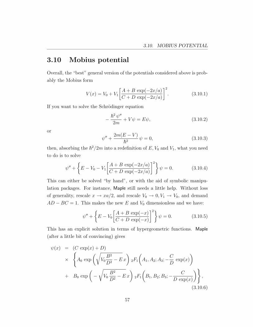
3.10. MOBIUS POTENTIAL
3.10 Mobius potential
Overall, the “best” general version of the potentials considered above is prob-
ably the Mobius form
V (x) = V0 + V1
[A+B exp(−2x/a)
C +D exp(−2x/a)
]2
. (3.10.1)
If you want to solve the Schrodinger equation
− ~2 ψ′′
2m+ V ψ = Eψ, (3.10.2)
or
ψ′′ +2m(E − V )
~2ψ = 0, (3.10.3)
then, absorbing the ~2/2m into a redefinition of E, V0 and V1, what you need
to do is to solve
ψ′′ +
E − V0 − V1
[A+B exp(−2x/a)
C +D exp(−2x/a)
]2ψ = 0. (3.10.4)
This can either be solved “by hand”, or with the aid of symbolic manipu-
lation packages. For instance, Maple still needs a little help. Without loss
of generality, rescale x → xa/2, and rescale V0 → 0, V1 → V0, and demand
AD −BC = 1. This makes the new E and V0 dimensionless and we have:
ψ′′ +
E − V0
[A+B exp(−x)
C +D exp(−x)
]2ψ = 0. (3.10.5)
This has an explicit solution in terms of hypergeometric functions. Maple
(after a little bit of convincing) gives
ψ(x) = (C exp(x) +D)
×
A0 exp
(√V0B2
D2− E x
)2F1
(A1, A2;A3;−C
Dexp(x)
)
+ B0 exp
(−√V0B2
D2− E x
)2F1
(B1, B2;B3;− C
D exp(x)
),
(3.10.6)
57

CHAPTER 3. KNOWN ANALYTIC RESULTS
where the suppressed arguments on the hypergeometric functions are:
A1 =1
2+
√V0B2
D2− E − 1
2
√1 +
4V0
C2D2−√V0
(1 +BC)2
C2D2− E;
(3.10.7)
A2 =1
2+
√V0B2
D2− E − 1
2
√1 +
4V0
C2D2+
√V0
(1 +BC)2
C2D2− E;
(3.10.8)
A3 = 1 + 2
√V0B2
D2− E;
(3.10.9)
and
B1 =1
2−√V0B2
D2− E − 1
2
√1 +
4V0
C2D2+
√V0A2
C2− E;
(3.10.10)
B2 =1
2−√V0B2
D2− E − 1
2
√1 +
4V0
C2D2−√V0A2
C2− E;
(3.10.11)
B3 = 1− 2
√V0B2
D2− E.
(3.10.12)
By looking up tabulated properties of the hypergeometric function one can
now determine the bound state eigenvalues, reflection and transmission co-
efficients, etc.
In general, the Mobius potential exhibits both bound and free states. (As it
must, since after all the way we have derived it is by showing that it is equiv-
alent to any of the Manning–Rosen, Poeschl–Teller, or Eckart potentials.)
When the potential energy has a minimum but goes asymptotically to some
higher finite value at x = +∞ and −∞, then some of the allowed energies
will be discrete values, corresponding to states for which the particle is bound
in the potential valley. For other ranges of energy, higher than the minimum
58

3.11. OTHER POTENTIALS:
of the two asymptotic values, all energies will be allowed, the particle being
free to travel to infinity.
For instance, consider the wave functions and allowed energies for a parti-
cle of mass m in a Mobius potential that is written in Poeschl–Teller form [59]
V (x) = V0 cosh2µtanh[(x− µL)/L] + tanh(µ)2. (3.10.13)
For V0 positive, this potential field has its minimum value (V = 0) at x = 0.
As x is increased positive, the potential increases to an asymptotic value
V0 exp(2µ) for x→ +∞; as x is made negative, V also rises to an asymptotic
value V0 exp(−2µ), for x→ −∞. Classically, since in this form the potential
is constrained to be positive semidefinite, the particle could not have a nega-
tive energy; for energies between zero and V0 exp(−2µ), (µ > 0), the particle
would oscillate back and forth in the potential valley; for energies between
V0 exp(−2µ) and V0 exp(2µ), the particle could come from −∞, be reflected
by the potential rise to the right of the minimum, and go back to −∞ and
for energies greater than V0 exp(2µ), the particle could move from −∞ to
+∞ or from +∞ to −∞ [59].
3.11 Other potentials:
Furthermore, we would like to at least mention some other potentials:
Morse (1929)
V (x) = V0 (1− exp(−[x− x0]/a))2. (3.11.1)
The Morse potential is actually a somewhat odd limit of the Mobius potential
as various parameters go to unity or zero. In terms of the Mobius potential
above we need V0 → 0, V1 → V0, A = B → 1, C → 1, D → 0, x→ x− x0.
Manning–Rosen (1933)
V (x) = B coth(x/d)− C cosech2(x/d). (3.11.2)
59

CHAPTER 3. KNOWN ANALYTIC RESULTS
Warning: The relevant citation [26] is only an abstract in a report of a
conference. To find it with online tools such as PROLA look up Phys. Rev. 44
(1933) 951, and then manually scan for abstract # 10. The form actually
given in the abstract is
V (x) = Aexp(−2x/b)
[1− exp(−x/b)]2+B
exp(−x/b)1− exp(−x/b)
, (3.11.3)
which you can manipulate into the form above by noting
1 + 2exp(−x/b)
1− exp(−x/b)=
1 + exp(−x/b)1− exp(−x/b)
,
=exp(x/2b) + exp(−x/2b)exp(x/2b)− exp(−x/2b)
= coth(x/2b),
(3.11.4)
and
coth2z = 1 + cosech2z. (3.11.5)
Note that the Manning–Rosen potential can be obtained from the Eckart
potential by the substitution
ξ = − exp(2x/a)→ + exp(−2x/a). (3.11.6)
In particular, Manning–Rosen can be written in the form
V (x) = A+B coth(x/a) + C coth2(x/a) ,
= A0 + [B0 + C0 coth(x/a)]2. (3.11.7)
We can get this from the general Mobius form of the Eckart potential by
appropriately choosing the parameters.
Hulthen (1942)
V (x) = V0exp(−x/a)
1− exp(−x/a). (3.11.8)
The Hulthen potential [70] is actually a special case of the Manning–Rosen
potential (A = 0). We can also get this from the general Mobius form of the
60

3.11. OTHER POTENTIALS:
Eckart potential by appropriately choosing the parameters.
Tietz (1963) One version of the Tietz potential [71] is:
V (x) = V0
(sinh([x− x0]/a)
sinh, cosh, exp(x/a)
)2
. (3.11.9)
We can get this from the general Mobius form of the Eckart potential by
appropriately choosing the parameters.
Hua (1990)
V (x) = V0
(1− exp(−2x/a)
1− q exp(−2x/a)
)2
. (3.11.10)
We can get this [117] from the general Mobius form of the Eckart potential
by appropriately choosing the parameters. We note
V (x) = V0
(exp(x/a)− exp(−x/a)
exp(x/a)− q exp(−x/a)
)2
,
= V1
(sinh(x/a)
(1 + q)sinh(x/a) + (1− q)cosh(x/a)
)2
. (3.11.11)
If q > 0 define 1 + q = coshθ and 1− q = sinhθ.
If q < 0 define 1− q = coshθ and 1 + q = sinhθ.
Then we see
V (x) = V1
(sinh(x/a)
sinh, cosh(x/a+ θ)
)2
(q 6= 0),
= V1
(sinh(x/a− θ)
sinh, cosh, exp(x/a)
)2
,
= (Tietz potential),
= V1
(A sinh(x/a) +B cosh(x/a)
sinh, cosh(x/a)
)2
,
= (Eckart potential or Manning–Rosen potential as appropriate).
(3.11.12)
So all of these potentials are either identical to the Mobius potential,
or special cases of the Mobius potential. To be historically accurate we
61

CHAPTER 3. KNOWN ANALYTIC RESULTS
should really just call this whole collection of potentials the Eckart potential,
as Eckhart seems to have been the first author to have given the general
form. Unfortunately other names are now in such common use that historical
accuracy is difficult (if not impossible) to recover.
3.12 Discussion
Let us summarize the results that we have obtained from this chapter.
In this chapter, we collected many known analytic results in a form
amenable to comparison with the general results we shall soon derive. In
addition, we introduced the concept of quasinormal modes. We shall use
these tools for comparing the bounds with known analytic results. More-
over, we reproduced some of the analytically known results, and showed (or
at least sketched) how to derive their scattering amplitudes, and so calcu-
late quantities such as the tunnelling probabilities and quasinormal modes
[QNM]. We did this explicitly for the delta–function potential, double–delta–
function potential, square potential barrier, tanh potential, sech2 potential,
asymmetric square-well potential, the Poeschl–Teller potential and its vari-
ants, and finally the Eckart–Rosen–Morse–Poeschl–Teller potential.
In addition, we are able to gain some deeper understanding by realizing
that the Eckart–Rosen–Morse–Poeschl–Teller potential is generally a Mobius
function of the variable exp(−2x/a). Furthermore, the Morse potential is
actually a specific limit of the Mobius potential as various parameters go to
unity or zero. We also demonstrate that the Hulthen potential is actually a
special case of the Manning–Rosen potential (A = 0).
As previously discussed, we have seen that a many of the “exactly solv-
able” potentials commonly encountered in the literature are actually the same
quantity in disguise. For instance, we devoted that all of these potentials are
either identical to the Mobius potential, or special cases of the Mobius po-
tential. Moreover, we should really just call this the Eckart potential, as he
seems to have been the first author to have given the general form. Unfor-
62

3.12. DISCUSSION
tunately other names are now in such common use that historical accuracy
is difficult (if not impossible) to recover.
Some potentials for which the transmission probability is explicitly known
Name Potential V (x) Transmission coefficient T = |t|2
Delta–function potential αδ(x)1
1 + (mα2/2E~2)
Double–delta–function αδ(x− L/2) + δ(x+ L/2) 1
1 +[
2mα~2k
cos (kL) + 12(2mα
~2k)2sin (kL)
]2Square potential barrier
V0 (for 0 ≤ x ≤ L)
0 (otherwise)4k2q2
4k2q2 + (k2 − q2)2 sin2(qL)
Tanh potential V+∞ tanh(x/L) 1−(
sinh[π(k−∞ − k+∞)L/2]sinh[π(k−∞ + k+∞)L/2]
)2
Sech2 potential Ve sech2(x/L) ≥ sech2
[√m2E
2L|Vpeak|~
]
Asymmetric Square-well
V1, x < a;
V2, a < x < b;
V3, b < x.
≥ 4k1k22k3
(k22 + k1k3)2
Table 3.1: This table shows some of the potentials for which exact ana-
lytic results are known, and summarizes key properties of the transmission
probabilities.
63

CHAPTER 3. KNOWN ANALYTIC RESULTS
Inter-relationships between various “exactly solvable” potentials
Name Potential V (x) Properties
Eckart (1930) − Aξ1−ξ −
Bξ(1−ξ)2 ; Eckart⇔ Rosen–Morse
where ξ = − exp(2x/a)
Rosen–Morse (1932) B tanh(x/d)− C sech2(x/d) Poeschl–Teller⇔ Rosen–Morse
Poeschl–Teller (1933) V0 cosh2µ Rosen–Morse ⇔ Poeschl–Teller
×tanh([x− µL]/L) + tanhµ2
Eckart–Rosen–Morse- A+B tanh(x/a+ θ) This is generally a Mobius function
-Poeschl–Teller +C tanh2(x/a+ θ) of the variable exp(−2x/a)
Mobius V1
[A+B exp(−2x/a)C+D exp(−2x/a)
]2
The “best” of these equivalent forms
Morse (1929) V0 (1− exp(−[x− x0]/a))2 Specific limit of the Mobius potential
Manning–Rosen (1933) B coth(x/d)− C cosech2(x/d) Obtained from Eckart by specific
substitution
Hulthen (1942) V0exp(−x/a)
1−exp(−x/a) A special case of Manning–Rosen
(A = 0)
Tietz (1963) V0
(sinh([x−x0]/a)
sinh,cosh,exp(x/a)
)2
Obtained from the general Mobius form
of Eckart by appropriately choosing
the parameters
Hua (1990) V0
(1−exp(−2x/a)
1−q exp(−2x/a)
)2
Eckart or Manning–Rosen
Table 3.2: This table shows the inter-connections between many “exactly
solvable” potentials. Many of these potentials are identical to each other,
though this may not always be obvious at first glance.
64

Chapter 4
Shabat–Zakharov systems
4.1 Introduction
In this chapter we shall present the general concept of the so-called “Shabat–
Zakharov systems”, (sometimes called “Zakharov–Shabat” systems). We
shall re-write the second-order Schrodinger equation as a particular set of two
coupled first order differential equations for which bounds can be (relatively)
easily established. In addition, we shall introduce the idea of the probability
current and demonstrate how to obtain the probability current density. We
shall then use the probability current (or probability flux) to describe the
flow of probability density.
Moreover, we shall present an “auxiliary condition” or “gauge condition”
that is used to relate two complex amplitudes a(x) and b(x) that we shall soon
introduce, and to eliminate da/dx in favour of db/dx. This allows us to write
d2ψ/dx2 in either of two equivalent forms, which is key to developing a 2× 2
matrix formalism. We shall represent the wave function in an inner product
form which is the explicit general (but formal) solution to the Schrodinger
equation. The general solution depends on three arbitrarily chosen functions
ϕ(x), ∆(x), and χ(x), and a path-ordered exponential matrix.
We shall consider path ordering as an “elementary” process to derive
the holy grail of ODE theory (complete quadrature, albeit formal, of the
65

CHAPTER 4. SHABAT–ZAKHAROV SYSTEMS
second-order linear ODE). We shall then use the freedom to independently
choose ϕ(x), ∆(x), and χ(x) to simplify the Bogoliubov coefficients (both
the relevant ODEs and the general bounds) as much as possible.
4.2 Ansatz
Consider the one-dimensional time-independent Schrodinger equation [37]–
[51]
− ~2
2m
d2
dx2ψ(x) + V (x) ψ(x) = E ψ(x). (4.2.1)
Introduce the notation
k(x)2 =2m[E − V (x)]
~2. (4.2.2)
So we are really just trying to solve
d2
dx2ψ(x) + k(x)2 ψ(x) = 0, (4.2.3)
or equivalently in the time domain
d2
dt2ψ(t) + ω(t)2 ψ(t) = 0. (4.2.4)
Motivated by the JWKB approximation,
ψ ≈ Aexp[i
∫k(x)]√
k(x)+B
exp[−i∫k(x)]√
k(x), (4.2.5)
the key idea is to re-write the second-order Schrodinger equation as a set
of two coupled first-order linear differential equations (for which bounds can
relatively easily be established). Systems of differential equations of this type
are often referred to as Shabat–Zakharov [53] systems. A similar represen-
tation of the Schrodinger equation is briefly discussed by Peierls [54] and
related representations are well-known, often being used without giving an
explicit reference (see e.g. [55]). However an exhaustive search has not un-
covered prior use of the particular representation presented here, (apart, of
66

4.2. ANSATZ
WKB (or JWKB) approximation: In general, WKB (or JWKB)
theory is a method for estimating the solution of a differential equation
whose highest derivative is multiplied by a small parameter ε. The
method of approximation is as follows [8]:
For a differential equation
εdny
dxn+ a(x)
dn−1
dxn−1+ ...+ k(x)
dy
dx+m(x)y = 0, (4.2.6)
assume a solution of the form of an asymptotic series expansion as
y(x) ≈ exp
[1
ε
∞∑n=0
εn Sn(x)
]. (4.2.7)
In the limit ε→ 0, substitution of the above ansatz into the differential
equation and canceling out the exponential terms allows one to solve
for an arbitrary number of terms Sn(x) in the expansion.
The most common application of this general formalism is to the
second-order differential equation presented in the standard form:
εd2y
dx2+m(x)y = 0. (4.2.8)
Keeping only the first two terms in the WKB approximation yields
y(x) ≈exp
±i∫ √
m(x) dx
4√m(x)
. (4.2.9)
It is this “standard” form of the WKB approximation that we will be
using extensively in this thesis.
course, from [88]), nor the idea of using the representation to place bounds
on one-dimensional scattering.
We will start by introducing two arbitrary auxiliary functions ϕ(x) and
67

CHAPTER 4. SHABAT–ZAKHAROV SYSTEMS
∆(x) which may be either real or complex, though we do demand that ϕ′(x) 6=0, and then defining
ψ(x) = a(x)exp(+iϕ+ i∆)√
ϕ′+ b(x)
exp(−iϕ− i∆)√ϕ′
. (4.2.10)
This representation effectively seeks to use quantities resembling the “phase
integral” wavefunctions as a basis for the true wavefunction [31]. We will
ultimately want to interpret a(x) and b(x) as “position-dependent WKB-like
coefficients”; in a scattering problem they can be thought of as “position-
dependent Bogoliubov coefficients”. This representation is of course ex-
tremely highly redundant, since one complex number ψ(x) has been traded
for two complex numbers a(x) and b(x), plus two essentially arbitrary auxil-
iary functions ϕ(x) and ∆(x).
To reduce this freedom, we introduce an “auxiliary condition” (or “aux-
iliary constraint”, or “gauge condition”):
d
dx
(a exp(i∆)√
ϕ′
)e+iϕ +
d
dx
(b exp(−i∆)√
ϕ′
)e−iϕ = χ(x) ψ(x). (4.2.11)
Here χ(x) is yet a third arbitrary function of position. It is allowed to be
complex, and may be zero. The original analysis, published in [88] corre-
sponds to the special case ∆(x) = 0 and χ(x) = 0. Subject to this gauge
condition,
dψ
dx= i√ϕ′ a(x) exp(+iϕ+ i∆)− b(x) exp(−iϕ− i∆)+ χ ψ. (4.2.12)
Repeated differentiation of this equation will soon lead to our desired result.
4.3 Probability current
We use the probability current (or probability flux) to describe the flow
of probability density. The following equation is use to describe the flow
of a fluid, a process which occurs all the way through physics and applied
mathematics [13]∂
∂tρ(x, t) = −∂J
∂x. (4.3.1)
68

4.3. PROBABILITY CURRENT
Definition (Zakharov–Shabat): We shall now turn to the study
of the non self adjoint Zakharov–Shabat problem. In a rather general
context, this may be viewed as the first order system of differential
equations in R defined by [7]:
h
(u′1(x, z)
u′2(x, z)
)=(
−iz A(x) exp(iS(x)/h)
−A(x) exp(−iS(x)/h) iz
)(u1(x, z)
u2(x, z)
),
(4.2.13)
where z is a complex eigenvalue parameter, and the prime denotes
differentiation with respect to x. This system appears (for instance)
when one wants to solve the non linear initial value problem given by
ih∂tψ +h2
2∂2xψ + |ψ|2 ψ = 0, (4.2.14)
ψ|t=0 = A(x) exp(iS(x)/h) , (4.2.15)
with the inverse scattering method [7].
The same sort of system of ODEs will also arise in our particular
problem: We are of course interested in the somewhat simpler problem
of solving the linear Schrodinger equation.
The above equation tells us that the rate of change in density is equal to the
negative of the difference between the amount of “stuff” (be it water, air, or
“probability”) flowing into the point and the amount flowing out. Now in
the context of the Schrodinger equation, we can write the probability density
in the following form
ρ(x, t) = |ψ(x, t)|2 = ψ∗ψ. (4.3.2)
69

CHAPTER 4. SHABAT–ZAKHAROV SYSTEMS
In quantum mechanics we can certainly describe the movement of particles,
however we also have an additional difficulty because our particles are not
classical. Therefore we can only talk about the probability of the particle
being at a certain place in time, now we can talk about a probability current
or flux. Consider the time–dependent Schrodinger Equation and its complex
conjugate:
i~∂ψ
∂t= Hψ(x, t) = − ~2
2m
∂2ψ
∂x2+ V ψ; (4.3.3)
−i~ ∂ψ∗
∂t= Hψ∗(x, t) = − ~2
2m
∂2ψ∗
∂x2+ V ψ∗. (4.3.4)
Now let us differentiate the probability density with respect to time
∂ρ
∂t=
∂
∂t
(ψ∗ψ
)=
(∂ψ∗
∂t
)ψ + ψ∗
(∂ψ
∂t
),
=~
2mi
(∂2ψ∗
∂x2ψ − ψ∗ ∂
2ψ
∂x2
)− V ψ∗ψ
i~+V ψ∗ψ
i~,
= − ∂
∂x
(~
2mi
(ψ∗
∂ψ
∂x− ∂ψ∗
∂xψ
)). (4.3.5)
Apply∂
∂tρ(x, t) +
∂
∂xJ (x, t) = 0. (4.3.6)
So we obtain the probability current density
J (x, t) =~
2mi
(ψ∗∂ψ
∂x− ∂ψ∗
∂xψ
). (4.3.7)
We can re-write this as
J (x, t) =~m
Im
(ψ∗∂ψ
∂x
). (4.3.8)
Here (~/m) is just a normalization (that is often set → 1 for convenience).
There is nothing really important in this normalization (unless we want to
calculate experimental numbers), so we might as well set
J (x, t) = Im
(ψ∗∂ψ
∂x
). (4.3.9)
70

4.4. SDE AS A FIRST ORDER SYSTEM
Now at this stage ϕ(x) and χ(x) are completely arbitrary possibly complex
functions subject only to the constraint ϕ′ 6= 0. For future use, compute the
probability current using our WKB-based ansatz in terms of a(x) and b(x):
J = Im
ψ∗
dψ
dx
,
= Im
ψ∗[i√ϕ′a(x) exp(+iϕ)− b(x) exp(−iϕ)+ χψ
],
(4.3.10)
= Re
√ϕ′
ϕ′∗[a(x) exp(+iϕ)− b(x) exp(−iϕ)]
[a(x)∗ exp(−iϕ∗) + b(x)∗ exp(+iϕ∗)]
+ Imχψ∗ψ, (4.3.11)
= Re
√ϕ′
ϕ′∗
[|a|2Ree+i(ϕ−ϕ∗) − |b|2Ree−i(ϕ−ϕ∗)
]+Im
√ϕ′
ϕ′∗
Imab∗ ei(ϕ+ϕ∗)
+ Imχψ∗ψ, (4.3.12)
= Re
√ϕ′
ϕ′∗
[|a|2Ree+2Im(ϕ) − |b|2Ree−2Im(ϕ)
]+Im
√ϕ′
ϕ′∗
Imab∗ e2iRe(ϕ)+ Imχψ∗ψ. (4.3.13)
4.4 SDE as a first order system
We now re-write the Schrodinger equation in terms of two coupled first-
order differential equations for these position-dependent WKB/Bogoliubov
coefficients a(x) and b(x). To do this we evaluate d2ψ/dx2 in two different
71

CHAPTER 4. SHABAT–ZAKHAROV SYSTEMS
ways, making repeated use of the gauge condition. First
d2ψ
dx2=
d
dx
(iϕ′√ϕ′ae+iϕ+i∆ − be−iϕ−i∆
+ χ ψ
), (4.4.1)
=(iϕ′)2
√ϕ′ae+iϕ+i∆ + be−iϕ−i∆
+iϕ′
d
dx
(a ei∆√ϕ′
)e+iϕ − d
dx
(b e−i∆√ϕ′
)e−iϕ
+i
ϕ′′√ϕ′ae+iϕ+i∆ − be−iϕ−i∆
+ χ′ ψ + χ ψ′, (4.4.2)
= − ϕ′2√ϕ′ae+iϕ+i∆ + be−iϕ−i∆
+iϕ′
2
d
dx
(a ei∆√ϕ′
)e+iϕ − χψ
+i
ϕ′′√ϕ′ae+iϕ+i∆ − be−iϕ−i∆
+ χ′ ψ + χ ψ′. (4.4.3)
But then
d2ψ
dx2= −ϕ′2 ψ +
2iϕ′√ϕ′
da
dxe+iϕ+i∆ − 2
√ϕ′∆′eiϕ+i∆a
−i ϕ′′√ϕ′be−iϕ−i∆ − iϕ′χψ + χ′ψ
+χ[i√ϕ′a(x)e+iϕ+i∆ − b(x)e−iϕ−i∆
+ χ ψ
]. (4.4.4)
So finally
d2ψ
dx2=
[χ2 + χ′ − (ϕ′)2
]ψ +
2iϕ′√ϕ′
da
dxe+iϕ+i∆
−2√ϕ′∆′eiϕ+i∆a− i [ϕ
′′ + 2χϕ′]√ϕ′
be−iϕ−i∆.
(4.4.5)
Now use the gauge condition to eliminate da/dx in favour of db/dx. This
permits us to write d2ψ/dx2 in either of the two equivalent forms
d2ψ
dx2=
[χ2 + χ′ − (ϕ′)2
]ψ − 2iϕ′
db
dx
e−iϕ−i∆√ϕ′
−2√ϕ′∆′e−iϕ−i∆b+ i [ϕ′′ + 2χϕ′] a
e+iϕ+i∆
√ϕ′
, (4.4.6)
72
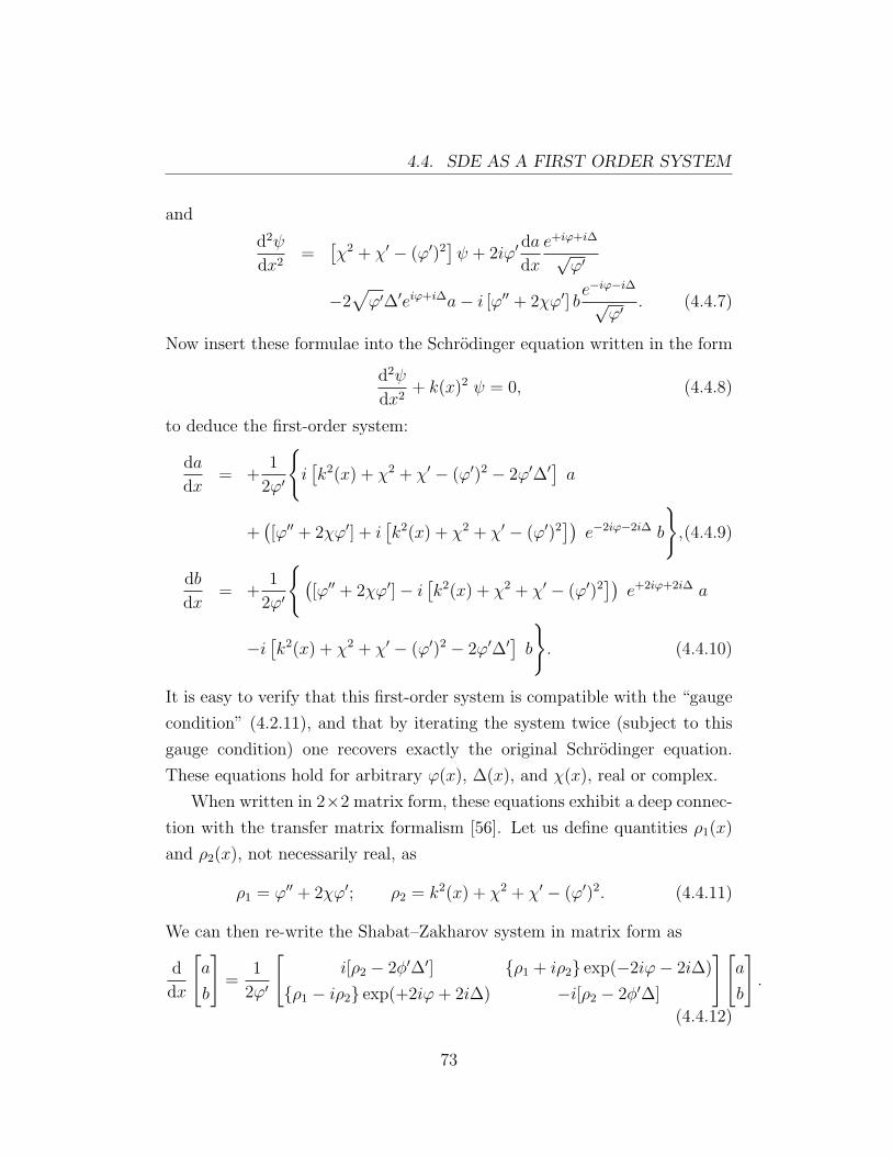
4.4. SDE AS A FIRST ORDER SYSTEM
and
d2ψ
dx2=
[χ2 + χ′ − (ϕ′)2
]ψ + 2iϕ′
da
dx
e+iϕ+i∆
√ϕ′
−2√ϕ′∆′eiϕ+i∆a− i [ϕ′′ + 2χϕ′] b
e−iϕ−i∆√ϕ′
. (4.4.7)
Now insert these formulae into the Schrodinger equation written in the form
d2ψ
dx2+ k(x)2 ψ = 0, (4.4.8)
to deduce the first-order system:
da
dx= +
1
2ϕ′
i[k2(x) + χ2 + χ′ − (ϕ′)2 − 2ϕ′∆′
]a
+([ϕ′′ + 2χϕ′] + i
[k2(x) + χ2 + χ′ − (ϕ′)2
])e−2iϕ−2i∆ b
,(4.4.9)
db
dx= +
1
2ϕ′
([ϕ′′ + 2χϕ′]− i
[k2(x) + χ2 + χ′ − (ϕ′)2
])e+2iϕ+2i∆ a
−i[k2(x) + χ2 + χ′ − (ϕ′)2 − 2ϕ′∆′
]b
. (4.4.10)
It is easy to verify that this first-order system is compatible with the “gauge
condition” (4.2.11), and that by iterating the system twice (subject to this
gauge condition) one recovers exactly the original Schrodinger equation.
These equations hold for arbitrary ϕ(x), ∆(x), and χ(x), real or complex.
When written in 2×2 matrix form, these equations exhibit a deep connec-
tion with the transfer matrix formalism [56]. Let us define quantities ρ1(x)
and ρ2(x), not necessarily real, as
ρ1 = ϕ′′ + 2χϕ′; ρ2 = k2(x) + χ2 + χ′ − (ϕ′)2. (4.4.11)
We can then re-write the Shabat–Zakharov system in matrix form as
d
dx
[a
b
]=
1
2ϕ′
[i[ρ2 − 2φ′∆′] ρ1 + iρ2 exp(−2iϕ− 2i∆)
ρ1 − iρ2 exp(+2iϕ+ 2i∆) −i[ρ2 − 2φ′∆]
][a
b
].
(4.4.12)
73

CHAPTER 4. SHABAT–ZAKHAROV SYSTEMS
This has the formal solution[a(xf )
b(xf )
]= E(xf , xi)
[a(xi)
b(xi)
], (4.4.13)
in terms of a generalized position-dependent “transfer matrix” [56]
E(xf , xi) =
P exp
(∫ xf
xi
1
2ϕ′
[i[ρ2 − 2ϕ′∆′] ρ1 + iρ2 e−2iϕ−2i∆
ρ1 − iρ2 e+2iϕ+2i∆ −i[ρ2 − 2ϕ′∆′]
]dx
),
(4.4.14)
where the symbol P denotes “path ordering”.
Path ordering: In theoretical physics, path–ordering is the proce-
dure (or meta-operator P) of ordering a product of many operators
according to the value of one chosen parameter [29]:
P [O1(σ1)O2(σ2)...On(σn)] = Op(1)(σp(1))Op(2)(σp(2))...Op(n)(σp(n)).
(4.4.15)
Here p : 1, 2, ..., n → 1, 2, ..., n is a permutation that orders the
parameters: σp(1) ≤ σp(2) ≤ ... ≤ σp(n). For instance
P [O1(4)O2(2)O3(3)O4(1)] := O4(1)O3(3)O2(2)O1(4). (4.4.16)
Equivalently if we were to be working in the time domain we would have
E(tf , ti) =
T exp
(∫ tf
ti
1
2ϕ′
[i[ρ2 − 2ϕ′∆′] ρ1 + iρ2 e−2iϕ−2i∆
ρ1 − iρ2 e+2iϕ+2i∆ −i[ρ2 − 2ϕ′∆′]
]dt
),
(4.4.17)
where T would now be the well-known “time ordering” operator (more usu-
ally encountered in quantum field theory) and we would now define
ρ1 = ϕ′′ + 2χϕ′; ρ2 = ω2(t) + χ2 − χ′ − (ϕ′)2, (4.4.18)
74

4.5. BOUNDING THE COEFFICIENTS A(X) AND B(X)
with ϕ, ∆, and χ now being arbitrary functions of t rather than x.
We can now write the wave function in inner product form
ψ(x) =1√ϕ′
[exp(+iϕ+ i∆); exp(−iϕ− i∆)
] [a(xi)
b(xi)
], (4.4.19)
to yield a formal but completely general solution for the Schrodinger equation
ψ(x) =1√ϕ′
[exp(+iϕ+ i∆); exp(−iϕ− i∆)
]E(x, x0)
[a(x0)
b(x0)
]. (4.4.20)
Explicitly
ψ(x) =1√ϕ′
[exp(+iϕ+ i∆); exp(−iϕ+ i∆)
](4.4.21)
P exp
(∫ x
x0
1
2ϕ′
[i[ρ2 − 2ϕ′∆′] ρ1 + iρ2 e−2iϕ−2i∆
ρ1 − iρ2 e+2iϕ+2i∆ −i[ρ2 − 2ϕ′∆′]
]dx
)[a(x0)
b(x0)
].
This is the explicit general solution to the Schrodinger equation. It depends
on the three arbitrarily chosen functions ϕ(x), ∆(x), and χ(x), and a path-
ordered exponential matrix. If you consider path ordering to be an “elemen-
tary” process, then this is indeed the holy grail of ODE theory (complete
quadrature, albeit formal, of the second-order linear ODE).
4.5 Bounding the coefficients a(x) and b(x)
From
da
dx= +
1
2ϕ′
i[k2(x) + χ2 + χ′ − (ϕ′)2 − 2ϕ′∆′
]a
+([ϕ′′ + 2χϕ′] + i
[k2(x) + χ2 + χ′ − (ϕ′)2
])e−2iϕ−2i∆ b
,
(4.5.1)
db
dx= +
1
2ϕ′
([ϕ′′ + 2χϕ′]− i
[k2(x) + χ2 + χ′ − (ϕ′)2
])e+2iϕ+2i∆ a
−i[k2(x) + χ2 + χ′ − (ϕ′)2 − 2ϕ′∆′
]b
, (4.5.2)
75

CHAPTER 4. SHABAT–ZAKHAROV SYSTEMS
we see
a∗da
dx= +
1
2ϕ′
i[k2(x) + χ2 + χ′ − (ϕ′)2 − 2ϕ′∆′
]a∗a
+([ϕ′′ + 2χϕ′] + i
[k2(x) + χ2 + χ′ − (ϕ′)2
])e−2iϕ−2i∆ a∗ b
.
(4.5.3)
Therefore (now assuming for the rest of this section that ϕ, ∆, χ are all real
and ϕ′ > 0)
a∗da
dx+a
da∗
dx=
Re([ϕ′′ + 2χϕ′] + i [k2(x) + χ2 + χ′ − (ϕ′)2]) e−2iϕ−2i∆ a∗ bϕ′
.
(4.5.4)
This implies
d|a|2
dx=
Re([ϕ′′ + 2χϕ′] + i [k2(x) + χ2 + χ′ − (ϕ′)2]) e−2iϕ−2i∆ a∗ bϕ′
.
(4.5.5)
But Re(A) ≤ |A|, so we have
d|a|2
dx≤∣∣([ϕ′′ + 2χϕ′] + i [k2(x) + χ2 + χ′ − (ϕ′)2]) e−2iϕ−2i∆ a∗ b
∣∣ϕ′
, (4.5.6)
implying
2|a|d|a|dx≤ | [ϕ
′′ + 2χϕ′] + i [k2(x) + χ2 + χ′ − (ϕ′)2] | |a| |b|ϕ′
. (4.5.7)
Thus
d|a|dx≤ | [ϕ
′′ + 2χϕ′] + i [k2(x) + χ2 + χ′ − (ϕ′)2] | |b|2ϕ′
, (4.5.8)
and so
d|a|dx≤
√[ϕ′′ + 2χϕ′]2 + [k2(x) + χ2 + χ′ − (ϕ′)2]2
2ϕ′|b|. (4.5.9)
Now if (as per our current assumption) ϕ, ∆, χ are all real, then it is easy
to check that
J = Im(ψ∗ψ′) = |a|2 − |b|2, (4.5.10)
76

4.5. BOUNDING THE COEFFICIENTS A(X) AND B(X)
so current conservation implies
|a|2 − |b|2 = 1. (4.5.11)
Ultimately, it is this equation that allows us to interpret a(x) and b(x) as
“position dependent Bogoliubov coefficients”.
In view of the relation between a(x) and b(x) we have |b| =√|a|2 − 1, so
that we can deduce
d|a|dx≤
√[ϕ′′ + 2χϕ′]2 + [k2(x) + χ2 + χ′ − (ϕ′)2]2
2ϕ′
√|a|2 − 1. (4.5.12)
But this inequality can now be integrated. For convenience let us define
ϑ =
√[ϕ′′ + 2χϕ′]2 + [k2(x) + χ2 + χ′ − (ϕ′)2]2
2ϕ′. (4.5.13)
Thend|a|dx≤ ϑ
√|a|2 − 1. (4.5.14)
But now ∫1√|a|2 − 1
d|a|dx
dx ≤∫ϑ dx, (4.5.15)
so that cosh−1 |a|
xf
xi≤∫ xf
xi
ϑ dx. (4.5.16)
Now apply the boundary conditions: as xi → −∞ we have chosen to set
things up so that we have a pure transmitted wave, so |b(−∞)| = 0 and
|a(−∞)| = 1. On the other hand as xf → +∞ we have chosen to set things
up so that a(x) and b(x) tend to α and β, the Bogoliubov coefficients we
are interested in calculating. Thus taking the double limit xi → −∞ and
xf → +∞ we see:
cosh−1 |α| ≤∫ +∞
−∞ϑ dx. (4.5.17)
That is
|α| ≤ cosh
∫ +∞
−∞ϑ dx
. (4.5.18)
77

CHAPTER 4. SHABAT–ZAKHAROV SYSTEMS
This is the central result of this thesis — it can be modified and rearranged
in a number of ways, and related inequalities can be derived under slightly
different hypotheses, but all the applications we are interested in will reduce
in one way or another to an application of this inequality or one of its close
variants.
For notational convenience, we often find it is useful to adopt the short-
hand ∮=
∫ +∞
−∞, (4.5.19)
since then
|α| ≤ cosh
∮ϑ dx
. (4.5.20)
From the normalization condition (4.5.11) we immediately deduce
|β| ≤ sinh
∮ϑ dx
. (4.5.21)
When translated into equivalent statements about transmission an reflection
probabilities, we find
T ≥ sech2
∮ϑ dx
, (4.5.22)
and
R ≤ tanh2
∮ϑ dx
. (4.5.23)
Now one of the the points of the exercise (and of this thesis) is to use
the freedom to independently choose ϕ(x), ∆(x), and χ(x) to simplify life
as much as possible. Here are a few special cases, chosen for their simplicity
and the lessons they teach us.
4.5.1 Case: ∆′ = ρ2/(2ϕ′)
No one can prevent us from choosing
∆′ =ρ2
2ϕ′, (4.5.24)
78

4.5. BOUNDING THE COEFFICIENTS A(X) AND B(X)
that is
∆′ =k2(x) + χ2 + χ′ − (ϕ′)2
2ϕ′, (4.5.25)
which implies
∆ =
∫k2(x) + χ2 + χ′ − (ϕ′)2
2ϕ′dx. (4.5.26)
Doing that greatly simplifies life since now the system of ODEs becomes
da
dx= +
1
2ϕ′
([ϕ′′ + 2χϕ′] + i
[k2(x) + χ2 + χ′ − (ϕ′)2
])e−2iϕ−2i∆ b
,
(4.5.27)
db
dx= +
1
2ϕ′
([ϕ′′ + 2χϕ′]− i
[k2(x) + χ2 + χ′ − (ϕ′)2
])e+2iϕ+2i∆ a
.
(4.5.28)
That is
d
dx
[a
b
]=
1
2ϕ′
[0 ρ1 + iρ2 exp(−2iϕ− 2i∆)
ρ1 − iρ2 exp(+2iϕ+ 2i∆) 0
][a
b
].
(4.5.29)
If you now let ϕ and χ be real, then the matrix above is Hermitian; unfor-
tunately this does not tell us all that much about the evolution operator.
(If we had i times a Hermitian operator appearing above, then the evolution
operator would have been unitary.) Using a specialization of the previous
argument, we can easily deduce
d|a|dt
=
√[ϕ′′ + 2χϕ′]2 + [k2(x) + χ2 + χ′ − (ϕ′)2]2
2|ϕ′||b|. (4.5.30)
We also have the same constraint
|a|2 − |b|2 = 1, (4.5.31)
and so deduce
d|a|dt
=
√[ϕ′′ + 2χϕ′]2 + [k2(x) + χ2 + χ′ − (ϕ′)2]2
2|ϕ′|√|a|2 − 1. (4.5.32)
79

CHAPTER 4. SHABAT–ZAKHAROV SYSTEMS
Defining
ϑ =
√[ϕ′′ + 2χϕ′]2 + [k2(x) + χ2 + χ′ − (ϕ′)2]2
2|ϕ′|, (4.5.33)
we haved|a|dt
= ϑ√|a|2 − 1. (4.5.34)
This inequality can now be integrated in the manner discussed above, though
doing so gives us no additional information.
4.5.2 Case: ∆ = −ϕ
No one can prevent us from choosing
∆(x) = −ϕ(x), (4.5.35)
in which case
da
dx= +
1
2ϕ′
i[k2(x) + χ2 + χ′ + (ϕ′)2
]a
+([ϕ′′ + 2χϕ′] + i
[k2(x) + χ2 + χ′ − (ϕ′)2
])b
, (4.5.36)
db
dx= +
1
2ϕ′
([ϕ′′ + 2χϕ′]− i
[k2(x) + χ2 + χ′ − (ϕ′)2
])a
−i[k2(x) + χ2 + χ′ + (ϕ′)2
]b
. (4.5.37)
The complicated phase structure has gone away, and we have
a∗da
dx= +
1
2ϕ′
i[k2(x) + χ2 + χ′ + (ϕ′)2
]a∗ a
+([ϕ′′ + 2χϕ′] + i
[k2(x) + χ2 + χ′ − (ϕ′)2
])a∗ b
,(4.5.38)
80

4.5. BOUNDING THE COEFFICIENTS A(X) AND B(X)
whence
a∗da
dx+ a
da∗
dx=
Re([ϕ′′ + 2χϕ′] + i [k2(x) + χ2 + χ′ − (ϕ′)2]) a∗ b2ϕ′
.
(4.5.39)
Perhaps more to the point, we can derive ODEs for the sums and differences:
d(a+ b)
dx= +
1
ϕ′
[ϕ′′ + 2χϕ′](a+ b) + 2i(ϕ′)2(a− b)
, (4.5.40)
d(a− b)dx
= +1
ϕ′
− i[k2(x) + χ2 + χ′
](a+ b)− [ϕ′′ + 2χϕ′](a− b)
.
(4.5.41)
that is
d[i(a+ b)]
dx= +
1
ϕ′
[ϕ′′ + 2χϕ′](a+ b) + 2(ϕ′)2[i(a− b)]
, (4.5.42)
d[i(a− b)]dx
= +1
ϕ′
[k2(x) + χ2 + χ′
](a+ b)− [ϕ′′ + 2χϕ′] [i(a− b)]
.
(4.5.43)
While this system of ODEs is somewhat simpler than those derived above,
we have not been able to extract any significant improvement on or previous
results in equations (4.5.13) and (4.5.18).
4.5.3 Case: ∆ = 0
We include this case for historical reasons, as it was the first generalization we
obtained of the original result published in [88]. The derivation is somewhat
simpler than the full ∆ 6= 0 discussion presented above, and the ultimate
bound we extract is no weaker.
We introduce an arbitrary auxiliary function ϕ(x) which may be either
real or complex, however we demand that ϕ′(x) 6= 0, and then define
ψ(x) = a(x)exp(+iϕ)√
ϕ′+ b(x)
exp(−iϕ)√ϕ′
. (4.5.44)
81

CHAPTER 4. SHABAT–ZAKHAROV SYSTEMS
Again, to trim down the number of degrees of freedom it is useful to impose
what can be thought of as a “gauge condition” (“auxiliary condition”)
d
dx
(a√ϕ′
)e+iϕ +
d
dx
(b√ϕ′
)e−iϕ = χ(x)ψ(x). (4.5.45)
Here χ is some arbitrary function of position. The original analysis in [88]
corresponds to the special case χ(x) = 0. Subject to this gauge condition,
dψ
dx= i√ϕ′a(x) exp(+iϕ)− b(x) exp(−iϕ)+ χψ. (4.5.46)
Now the Schrodinger equation can be rewritten in terms of two coupled
first-order differential equations for these position-dependent Bogoliubov co-
efficients. We have to calculate d2ψ/dx2 making repeated use of the gauge
condition:
d2ψ
dx2=
d
dx
(iϕ′√ϕ′ae+iϕ − be−iϕ+ χψ
), (4.5.47)
=(iϕ′)2
√ϕ′ae+iϕ + be−iϕ+ iϕ′
d
dx
(a√ϕ′
)e+iϕ − d
dx
(b√ϕ′
)e−iϕ
+i
ϕ′′√ϕ′ae+iϕ − be−iϕ+ χ′ψ + χψ′, (4.5.48)
= − ϕ′2√ϕ′ae+iϕ + be−iϕ+ iϕ′
2
d
dx
(a√ϕ′
)e+iϕ − χψ
+i
ϕ′′√ϕ′ae+iϕ − be−iϕ+ χ′ ψ + χψ′, (4.5.49)
= −ϕ′2ψ +2iϕ′√ϕ′
da
dxe+iϕ − i ϕ
′′√ϕ′be−iϕ − iϕ′χψ + χ′ψ
+χ[i√ϕ′ a(x)e+iϕ − b(x)e−iϕ+ χψ
], (4.5.50)
= [χ2 + χ′ − (ϕ′)2]ψ +2iϕ′√ϕ′
da
dxe+iϕ − i [ϕ
′′ + 2χϕ′]√ϕ′
be−iϕ. (4.5.51)
Now use the gauge condition to eliminate da/dx in favour of db/dx. Finally,
82

4.5. BOUNDING THE COEFFICIENTS A(X) AND B(X)
this permits us to write d2ψ/dx2 in either of the two equivalent forms
d2ψ
dx2= [χ2 + χ′ − (ϕ′)2]ψ − 2iϕ′
db
dx
e−iϕ√ϕ′
+ i[ϕ′′ + 2χϕ′] ae+iϕ
√ϕ′
;
(4.5.52)
= [χ2 + χ′ − (ϕ′)2]ψ + 2iϕ′da
dx
e+iϕ
√ϕ′− i[ϕ′′ + 2χϕ′] b
e−iϕ√ϕ′.
(4.5.53)
Now insert these formulae into the Schrodinger equation written in the form
d2ψ
dx2= −k(x)2ψ ≡ −2m[E − V (x)]
~2ψ, (4.5.54)
to deduce
da
dx= +
1
2ϕ′
[ϕ′′ + 2χϕ′] b exp(−2iϕ)
+i [k2(x) + χ2 + χ′ − (ϕ′)2] (a+ b exp(−2iϕ))
,
(4.5.55)
db
dx= +
1
2ϕ′
[ϕ′′ + 2χϕ′] a exp(+2iϕ)
−i [k2(x) + χ2 + χ′ − (ϕ′)2] (b+ a exp(+2iϕ))
.
(4.5.56)
It is (again) easy to verify that this first-order system is compatible with the
“gauge condition” (4.5.45), and that by iterating the system twice (subject to
this gauge condition) one recovers exactly the orginal Schrodinger equation.
These equations hold for arbitrary ϕ and χ, real or complex, and when
written in matrix form, exhibit a deep connection with the transfer matrix
formalism [56]. Let us define quantities ρ1(x) and ρ2(x), not necessarily real,
as
ρ1 = ϕ′′ + 2χϕ′; ρ2 = k2(x) + χ2 + χ′ − (ϕ′)2. (4.5.57)
83

CHAPTER 4. SHABAT–ZAKHAROV SYSTEMS
We can then re-write the Shabat–Zakharov system in matrix form as
d
dx
[a
b
]=
1
2ϕ′
[iρ2 ρ1 + iρ2 exp(−2iϕ)
ρ1 − iρ2 exp(+2iϕ) −iρ2
][a
b
].
(4.5.58)
This has the formal solution[a(xf )
b(xf )
]= E(xf , xi)
[a(xi)
b(xi)
], (4.5.59)
in terms of a generalized position-dependent “transfer matrix” [56]
E(xf , xi) =
P exp
(∫ xf
xi
1
2ϕ′
[iρ2 ρ1 + iρ2 exp(−2iϕ)
ρ1 − iρ2 exp(+2iϕ) −iρ2
]dx
),
(4.5.60)
where the symbol P denotes “path ordering”. (See the boxed text earlier
in this chapter for details.) Now we can write the wave function in inner
product form
ψ(x) =1√ϕ′
[exp(+iϕ); exp(−iϕ)
] [ a(xi)
b(xi)
], (4.5.61)
and where [a(x)
b(x)
]= E(x, x0)
[a(x0)
b(x0)
]. (4.5.62)
Therefore
ψ(x) =1√ϕ′
[exp(+iϕ); exp(−iϕ)
]E(x, x0)
[a(x0)
b(x0)
], (4.5.63)
to yield a formal but completely general solution for the Schrodinger equation
√ϕ′ψ(x) =
[exp(+iϕ); exp(−iϕ)
]E(x, x0)
[a(x0)
b(x0)
]. (4.5.64)
84

4.6. DISCUSSION
Explicitly
ψ(x) =1√ϕ′
[exp(+iϕ); exp(−iϕ)
]×P exp
(∫ x
x0
1
2ϕ′
[iρ2 ρ1 + iρ2 exp(−2iϕ)
ρ1 − iρ2 exp(+2iϕ) −iρ2
]dx
)
×
[a(x0)
b(x0)
]. (4.5.65)
This is the explicit general solution to the Schrodinger equation. It depends
on the two arbitrarily chosen functions ϕ(x) and χ(x) and a path-ordered
exponential matrix. If you consider path ordering to be an “elementary” pro-
cess, then this is (again) the holy grail of ODE theory (complete quadrature,
albeit formal, of the second-order linear ODE).
The development of bounds automatically follows as in the previous dis-
cussion, and we can without further calculation assert that equations (4.5.13)
and (4.5.18) hold in this situation as well.
4.6 Discussion
There are several ways to derive a number of rigourous bounds on transmis-
sion probabilities (and reflection probabilities and Bogoliubov coefficients)
for one-dimensional scattering problems. The derivation of these bounds
generally proceeds by rewriting the Schrodinger equation in terms of some
equivalent system of first-order equations, and then analytically bounding
the growth of certain quantities related to the net flux of particles as one
sweeps across the potential. In this chapter we obtained a number of sig-
nificant bounds, considerably stronger than those in [88], of both theoretical
and practical interest.
Even though the calculations we have presented are sometimes somewhat
tedious, we feel however, they are more than worth the effort — since there
is a fundamental lesson to be learnt from them. Technically, we demon-
strated that the Schrodinger equation can be written as a Shabat–Zakharov
85

CHAPTER 4. SHABAT–ZAKHAROV SYSTEMS
system, which can then be re-written in 2 × 2 matrix form. We rearranged
this formation in terms of a generalized position-dependent “transfer ma-
trix” involving the symbol P which denotes “path ordering”. Therefore the
wavefunction ψ(x) can be written in inner product form. This is the explicit
general solution to the Schrodinger equation. It depends on the three arbi-
trarily chosen functions ϕ(x), ∆(x), and χ(x) and a path-ordered exponential
matrix. If one considers path ordering to be an “elementary” process, then
this is the holy grail of ODE theory (complete quadrature, albeit formal, of
the second-order linear ODE). We have seen that it is often convenient to use
the freedom to independently choose ϕ(x), ∆(x), and χ(x) to simplify life
as much as possible. Furthermore, we have considered a few special cases.
For instance, case ∆′ = ρ2/(2ϕ′), case ∆ = ϕ, and case ∆ = 0. The bounds
that we have derived on the Bogoliubov coefficients α and β, and on the
transmission and reflection probabilities T and R, are the key results of this
thesis — the next few chapters will be devoted to developing several variants
of these bounds, developing independent proofs that might ultimately lead
to new bounds, and developing various applications of these bounds.
86
Chapter 5
First derivation of the bounds
5.1 Introduction
In this chapter we shall review the analysis of [88], developing various tech-
niques for estimating the scattering properties. We shall review and briefly
describe some very general bounds for reflection and transmission coefficients
for one-dimensional potential scattering, and then indicate how the results
of this thesis extend and expand on the earlier results. Equivalently, these
results may be phrased as general bounds on the Bogoliubov coefficients, or
statements about the transfer matrix [88].
Finally, we shall re-demonstrate the use of Shabat–Zakharov system of
ODEs (now in a greatly simplified context) to derive a first elementary bound
on the transmission, reflection, and Bogoliubov coefficients.
5.2 Shabat–Zakharov systems
Consider the one-dimensional time-independent Schrodinger equation [37]–
[51]
− ~2
2m
d2
dx2ψ(x) + V (x) ψ(x) = E ψ(x). (5.2.1)
87

CHAPTER 5. FIRST DERIVATION OF THE BOUNDS
If the potential asymptotes to a constant,
V (x→ ±∞)→ V±∞, (5.2.2)
then in each of the two asymptotic regions there are two independent solu-
tions to the Schrodinger equation
ψ(±i;±∞;x) ≈ exp(±ik±∞x)√k±∞
. (5.2.3)
Here the ±i distinguishes right-moving modes e+ikx from left-moving modes
e−ikx, while the ±∞ specifies which of the asymptotic regions we are in.
Furthermore
k±∞ =
√2m(E − V±∞)
~. (5.2.4)
To even begin to set up a scattering problem the minimum requirements are
that the potential asymptote to some constant, and this assumption will be
made henceforth.
The so-called Jost solutions [52] are exact solutions J±(x) of the Schrodinger
equation that satisfy
J+(x→ +∞)→ exp(+ik+∞x)√k+∞
, (5.2.11)
J−(x→ −∞)→ exp(−ik−∞x)√k−∞
, (5.2.12)
and
J+(x→ −∞)→ αexp(+ik−∞x)√
k−∞+ β
exp(−ik−∞x)√k−∞
, (5.2.13)
J−(x→ +∞)→ α∗exp(−ik+∞x)√
k+∞+ β∗
exp(+ik+∞x)√k+∞
. (5.2.14)
Here α and β are the (right-moving) Bogoliubov coefficients, which are re-
lated to the (right-moving) reflection and transmission amplitudes by
r =β
α; t =
1
α. (5.2.15)
88

5.2. SHABAT–ZAKHAROV SYSTEMS
Definition (Jost solutions): If we were working in three dimensions
with radial symmetry then we would study the solution of the radial
Schrodinger equation [110]
d2f(r, k)
dr2+ (k2 − V (r)) f(r, k) = 0 , (5.2.5)
with the asymptotic conditions
limr→+∞
f(r ± k) exp(±ikr) = 1, (5.2.6)
the so-called “Jost solutions”. In one dimension we would consider a
formally identical equation for the full wave-function, now with bound-
ary conditions at both x → +∞ and x → −∞. In addition, we now
introduce the function
E(r, z) = exp(±ikr)f(r,±k). (5.2.7)
which is also called a “Jost solution”, and which satisfies the differen-
tial equation
d2E(r, z)
dr2− z dE(r, z)
dr− V (r)E(r, z) = 0, (5.2.8)
with the following condition at infinity
limr→+∞
E(r, z) = 1, (5.2.9)
where
z = ±2ik. (5.2.10)
These conventions correspond to an incoming flux of right-moving particles
(incident from the left) being partially transmitted and partially scattered.
The left-moving Bogoliubov coefficients are just the complex conjugates of
89
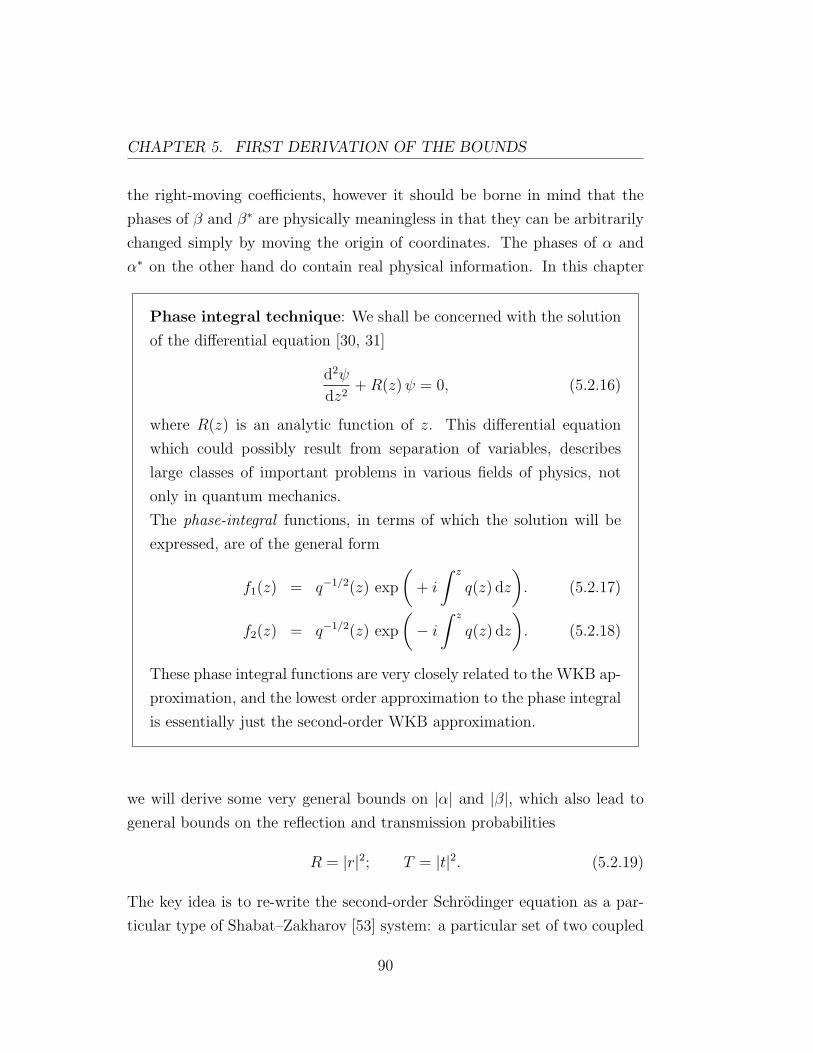
CHAPTER 5. FIRST DERIVATION OF THE BOUNDS
the right-moving coefficients, however it should be borne in mind that the
phases of β and β∗ are physically meaningless in that they can be arbitrarily
changed simply by moving the origin of coordinates. The phases of α and
α∗ on the other hand do contain real physical information. In this chapter
Phase integral technique: We shall be concerned with the solution
of the differential equation [30, 31]
d2ψ
dz2+R(z)ψ = 0, (5.2.16)
where R(z) is an analytic function of z. This differential equation
which could possibly result from separation of variables, describes
large classes of important problems in various fields of physics, not
only in quantum mechanics.
The phase-integral functions, in terms of which the solution will be
expressed, are of the general form
f1(z) = q−1/2(z) exp
(+ i
∫ z
q(z) dz
). (5.2.17)
f2(z) = q−1/2(z) exp
(− i∫ z
q(z) dz
). (5.2.18)
These phase integral functions are very closely related to the WKB ap-
proximation, and the lowest order approximation to the phase integral
is essentially just the second-order WKB approximation.
we will derive some very general bounds on |α| and |β|, which also lead to
general bounds on the reflection and transmission probabilities
R = |r|2; T = |t|2. (5.2.19)
The key idea is to re-write the second-order Schrodinger equation as a par-
ticular type of Shabat–Zakharov [53] system: a particular set of two coupled
90

5.2. SHABAT–ZAKHAROV SYSTEMS
first-order differential equations for which bounds can be easily established.
A similar representation of the Schrodinger equation is briefly discussed by
Peierls [54] and related representations are well-known, often being used with-
out giving an explicit reference (see e.g. [55]). However an exhaustive search
has not uncovered prior use of the particular representation of this chapter,
nor the idea of using the representation to place bounds on one-dimensional
scattering.
Scattering matrix: In physics, the scattering matrix (or S-matrix)
relates the initial state and the final state for an interaction of parti-
cles. It is used in quantum mechanics, scattering theory and quantum
field theory. In addition, it can also denote an infinite-dimensional
matrix (or operator) that expresses the state of a scattering system
consisting of waves or particles or both in the far future in terms of
its state in the remote past; also called the S-matrix. In the case of
electromagnetic (or acoustic) waves, it connects the intensity, phase,
and polarization of the outgoing waves in the far field at various an-
gles to the direction and polarization of the beam pointed toward an
obstacle [33, 34].
Definition (Auxiliary functions): They are not a rigorously de-
fined type of function. In contrast, these functions are either explic-
itly constructed, or at least shown to exist, and are used to provide
a formal solution to some assumed hypothesis, or otherwise prove the
result in question. Devising an auxiliary function during the course of
a proof in order to prove the result is not a technique exclusive to any
particular branch of mathematics [103].
91

CHAPTER 5. FIRST DERIVATION OF THE BOUNDS
Definition (Gauge conditions or Gauge fixing): Indicates a
mathematical scheme for coping with redundant degrees of freedom
in field variables, most commonly in the physics of gauge theories. In
Abelian or non-Abelian gauge theories one represents each physically
distinct configuration of the system as an equivalence class of detailed
local field configurations. Any two detailed configurations in the same
equivalence group are related by a gauge transformation, equivalent
to a shear along unphysical axes in configuration space [104].
In the context of the current thesis things are somewhat simpler.
There is a redundancy, which is eliminated by our “gauge condition”,
but one does not have to deal with the full complexity of an actual
“gauge theory” in the sense of particle physics.
We start by introducing an arbitrary auxiliary function ϕ(x) which may
be either real or complex, though we do demand that ϕ′(x) 6= 0, and then
defining
ψ(x) = a(x)exp(+iϕ)√
ϕ′+ b(x)
exp(−iϕ)√ϕ′
. (5.2.20)
This representation effectively seeks to use quantities resembling the “phase
integral” wavefunctions as a basis for the true wavefunction [72]. This rep-
resentation is of course highly redundant, since one complex number ψ(x)
has been traded for two complex numbers a(x) and b(x) plus an essentially
arbitrary auxiliary function ϕ(x). In order for this representation to be most
useful it is best to arrange things so that a(x) and b(x) asymptote to con-
stants at spatial infinity, which we shall soon see implies that we should pick
the auxiliary function to satisfy
ϕ′(x)→ k±∞ as x→ ±∞. (5.2.21)
To trim down the number of degrees of freedom it is useful to impose a “gauge
92

5.2. SHABAT–ZAKHAROV SYSTEMS
condition”
d
dx
(a√ϕ′
)e+iϕ +
d
dx
(b√ϕ′
)e−iϕ = 0. (5.2.22)
Subject to this gauge condition,
dψ
dx= i√ϕ′ a(x) exp(+iϕ)− b(x) exp(−iϕ) . (5.2.23)
We now re-write the Schrodinger equation in terms of two coupled first-order
differential equations for these position-dependent Bogoliubov coefficients.
To do this note that
d2ψ
dx2=
d
dx
(iϕ′√ϕ′ae+iϕ − be−iϕ
), (5.2.24)
=(iϕ′)2
√ϕ′ae+iϕ + be−iϕ
+ iϕ′
d
dx
(a√ϕ′
)e+iϕ − d
dx
(b√ϕ′
)e−iϕ
+ i
ϕ′′√ϕ′ae+iϕ − be−iϕ
, (5.2.25)
= − ϕ′2√ϕ′ae+iϕ + be−iϕ
+
2iϕ′√ϕ′
da
dxe+iϕ − i ϕ
′′√ϕ′be−iϕ , (5.2.26)
= − ϕ′2√ϕ′ae+iϕ + be−iϕ
− 2iϕ′√
ϕ′db
dxe−iϕ + i
ϕ′′√ϕ′ae+iϕ. (5.2.27)
(The last two relations use the “gauge condition”.) Now insert these formulae
into the Schrodinger equation written in the form
d2ψ
dx2= −k(x)2 ψ ≡ −2m(E − V (x))
~2ψ, (5.2.28)
93

CHAPTER 5. FIRST DERIVATION OF THE BOUNDS
to deduce
da
dx= +
1
2ϕ′
ϕ′′ b exp(−2iϕ)
+i[k2(x)− (ϕ′)2
](a+ b exp(−2iϕ))
, (5.2.29)
db
dx= +
1
2ϕ′
ϕ′′ a exp(+2iϕ)
−i[k2(x)− (ϕ′)2
](b+ a exp(+2iϕ))
. (5.2.30)
It is easy to verify that this first-order system is compatible with the “gauge
condition” (5.2.22), and that by iterating the system twice (subject to this
gauge condition) one recovers exactly the original Schrodinger equation.
These equations hold for arbitrary ϕ, real or complex, and when written
in matrix form, exhibit a deep connection with the transfer matrix formal-
ism [73].
5.3 Bounds
To obtain our bounds on the Bogoliubov coefficients we start by restrict-
ing attention to the case that ϕ(x) is a real function of x. (Since ϕ is an
essentially arbitrary auxiliary function this is not a particularly restrictive
condition). Under this assumption the probability current is
J = Im
ψ∗
dψ
dx
=|a|2 − |b|2
. (5.3.1)
Now at x ∼ +∞ the wavefunction is purely right-moving and normalized to
1, because we are considering one-dimensional Jost solutions [52]. Then for
all x we have a conserved quantity
|a|2 − |b|2 = 1. (5.3.2)
94

5.3. BOUNDS
It is this result that makes it useful to interpret a(x) and b(x) as position-
dependent Bogoliubov coefficients relative to the auxiliary function ϕ(x). Now
use the fact thatd|a|dx
=1
2|a|
(a∗
da
dx+ a
da∗
dx
), (5.3.3)
and use equation (5.2.29) to obtain
d|a|dx
=1
2|a|1
2ϕ′
(ϕ′′ [a∗b exp(−2iϕ) + ab∗ exp(+2iϕ)]
+i[k2 − (ϕ′)2] [a∗b exp(−2iϕ)− ab∗ exp(+2iϕ)]).
(5.3.4)
That is
d|a|dx
=1
2|a|1
2ϕ′Re
([ϕ′′ + i[k2 − (ϕ′)2]
][a∗b exp(−2iϕ)]
).
(5.3.5)
The right hand side can now be bounded from above, by systematically using
Re(A B) ≤ |A| |B|. This leads to
d|a|dx≤
√(ϕ′′)2 + [k2 − (ϕ′)2]2
2|ϕ′||b|. (5.3.6)
It is essential that ϕ be real to have | exp(−2iϕ)| = 1 which is the other key
ingredient above. Now define the non-negative quantity
ϑ = ϑ[ϕ(x), k(x)] ≡
√(ϕ′′)2 + [k2(x)− (ϕ′)2]2
2|ϕ′|, (5.3.7)
and use the conservation law (5.3.2) to write
d|a|dx≤ ϑ
√|a|2 − 1. (5.3.8)
Integrate this inequalitycosh−1 |a|
∣∣xf
xi≤∫ xf
xi
ϑ dx. (5.3.9)
95
CHAPTER 5. FIRST DERIVATION OF THE BOUNDS
Taking limits as xi → −∞ and xf → +∞
cosh−1 |α| ≤∫ +∞
−∞ϑ dx. (5.3.10)
That is
|α| ≤ cosh
(∫ +∞
−∞ϑ dx
). (5.3.11)
Which automatically implies
|β| ≤ sinh
(∫ +∞
−∞ϑ dx
). (5.3.12)
Since this result holds for all real choices of the auxiliary function ϕ(x),
(subject only to ϕ′ 6= 0 and ϕ′ → k±∞ as x→ ±∞), it encodes an enormously
wide class of bounds on the Bogoliubov coefficients. When translated to
reflection and transmission coefficients the equivalent statements are
T ≥ sech2
(∫ +∞
−∞ϑ dx
), (5.3.13)
and
R ≤ tanh2
(∫ +∞
−∞ϑ dx
). (5.3.14)
We shall soon turn this general result into more specific theorems in chapter 6.
5.4 Transfer matrix representation
The system of equations (5.2.29)–(5.2.30) can also be written in matrix form.
It is convenient to define
ρ ≡ ϕ′′ + i[k2(x)− (ϕ′)2]. (5.4.6)
Then
d
dx
[a
b
]=
1
2ϕ′
[iIm[ρ] ρ exp(−2iϕ)
ρ∗ exp(+2iϕ) −iIm[ρ]
][a
b
]. (5.4.7)
96

5.4. TRANSFER MATRIX REPRESENTATION
Transfer matrix formalism: This is most commonly used in optics
and acoustics to analyze the propagation of electromagnetic or acous-
tic waves through a stratified (layered) medium. In those situations,
the stack layers are normal to the z axis and the field within one layer
can be represented as the superposition of a left and right traveling
wave with wave number k [32],
E(z) = Er exp(ikz) + El exp(−ikz), (5.4.1)
We represent the field as the vector (E(z), F (z)), where
F (z) = ikEr exp(ikz)− ikEl exp(−ikz). (5.4.2)
The propagation over a distance L into the positive z direction is
described by the matrix
M =
[cos(kL) 1
ksin(kL)
−k sin(kL) cos(kL)
], (5.4.3)
and [E(z + L)
F (z + L)
]= M ×
[E(z)
F (z)
]. (5.4.4)
The system transfer matrix is then built up by repeated multiplication
Ms = MN × · · · ×M2 ×M1. (5.4.5)
A very similar formalism applies to the one-dimensional Schrodinger
equation, and the “path ordered” exponentials discussed in the body
of the thesis are effectively transfer matrices built out of an infinite
number of infinitesimally small steps.
97
CHAPTER 5. FIRST DERIVATION OF THE BOUNDS
This has the formal solution[a(xf )
b(xf )
]= E(xf , xi)
[a(xi)
b(xi)
], (5.4.8)
in terms of a generalized position-dependent “transfer matrix” [73]
E(xf , xi) =
P exp
(∫ xf
xi
1
2ϕ′
[iIm[ρ] ρ exp(−2iϕ)
ρ∗ exp(+2iϕ) −iIm[ρ]
][a
b
]dx
),
(5.4.9)
where the symbol P denotes “path ordering”. In particular, if we take
xi → −∞ and xf → +∞ we obtain a formal but exact expression for the
Bogoliubov coefficients[α β∗
β α∗
]= E(∞,−∞) =
P exp
(∫ ∞−∞
1
2ϕ′
[iIm[ρ] ρ exp(−2iϕ)
ρ∗ exp(+2iϕ) −iIm[ρ]
]dx
).
(5.4.10)
The matrix E is not unitary, though it does have determinant 1. It is in fact
an element of the group SU(1, 1). Taking
σz =
[+1 0
0 −1
], (5.4.11)
then (σz)2 = +I, and defining E† = (E∗)T , it is easy to see
E†σzE = σz. (5.4.12)
This is the analog of the invariance of the Minkowski metric for Lorentz
transformations in SO(3, 1).
98

5.5. DISCUSSION
Complex structure: There is a minor (non-propagating) error in
the analysis of [88]. If we define the “complex structure” J by
J =
[0 1
−1 0
], (5.4.13)
then J2 = −I and it is claimed in [88] that
E† = JEJ. (5.4.14)
This assertion is simply an error. Fortunately this is a side issue, and
the error does not affect the rest of the argument.
5.5 Discussion
In this chapter we have re-cast, re-analyzed, and described the first derivation
of scattering bounds as presented in [88]. The formalism as developed here
works in terms of one free function ϕ(x). In other parts of this thesis we have
established generalized bounds; some in terms of two arbitrary functions ϕ(x)
and χ(x), and some in terms of three arbitrary functions ϕ(x), ∆(x), and
χ(x). The derivation of the present chapter is noteworthy because of its
brevity and simplicity — and this chapter has acted as a “seed”, suggesting
and hinting at generalizations that have ultimately become the content of
the previous chapter. Of course, the “simple” calculation reported in this
chapter is also the seed for the various published journal articles that have
already arisen from this thesis, articles which are displayed in the appendices
to the thesis.
99

CHAPTER 5. FIRST DERIVATION OF THE BOUNDS
100

Chapter 6
Bounds: Special cases
In this chapter we shall deal with some specific cases of these general bounds
and develop a number of interesting specializations. We shall collect together
a large number of results that otherwise appear quite unrelated, including re-
flection above and below the barrier. We have divided the special case bounds
we consider into five sub-cases: Special cases 1–4, and “future directions”.
6.1 Bounds: Special case 1
We now reproduce the bounds of special case 1 in [88].
Suppose now that the potential satisfies V+∞ = V−∞. Also, choose the
phase function ϕ(x) to be ϕ = k∞x and take χ = 0. We also require k∞ 6= 0,
that is E > V±∞. This is the special case discussed in a different context by
Peierls [54]. Then the evolution equations simplify tremendously.
We consider the quantity
ϑ[k(x), ϕ(x), χ] =
√(ϕ′′ + 2χϕ′)2 + [k2(x) + χ2 + χ′ − (ϕ′)2]2
2|ϕ′|, (6.1.1)
which represents the generalization that we derived earlier in this thesis,
in equation (4.5.13), of the bound reported in [88]. When ϕ = k∞x, then
101
CHAPTER 6. BOUNDS: SPECIAL CASES
ϕ′′ = 0, and if we additionally choose χ = 0, then this simplifies to
ϑ[k(x), ϕ(x), χ] =
√[k2(x)− (k∞)2]2
2|k∞|=|k2 − k2
∞|2|k∞|
. (6.1.2)
Inserting this into our general bound now reproduces case 1 of [88] as desired.
Furthermore, we can calculate
ϑ[k(x), ϕ(x), χ] =|k2 − k2
∞|2|k∞|
=|2m(E − V )|
2~2|k∞|− |2m(E − V∞)|
2~2|k∞|,
=m|V (x)− V∞|
~2k∞.
From the previous chapters 4 and 5, we derive
T ≥ sech2
(∫ +∞
−∞ϑ[k, ϕ, χ] dx
), (6.1.3)
when ~k∞ =√
2m(E − V∞), then k∞ =
√2m(E − V∞)
~. Now we can find
ϑ[k(x), ϕ(x), χ] =
(m|V (x)− V∞|
~2
)(~√
2m(E − V∞)
),
=m|V (x)− V∞|
~√
2m(E − V∞)=
1
~
√m
2(E − V∞)|V (x)− V∞|.
(6.1.4)
Therefore,
T ≥ sech2
(∫ +∞
−∞ϑ[k, ϕ, χ] dx
),
= sech2
(∫ +∞
−∞
1
~
√m
2(E − V∞)|V (x)− V∞| dx
),
= sech2
(1
~
√m
2(E − V∞)
∫ +∞
−∞|V − V∞| dx
),
as desired.
Similarly one can find R in terms of [k(x), ϕ(x), χ]. Note
ϑ→ |k2 − k2
∞|2k∞
=m|V (x)− V∞|
~2k∞. (6.1.5)
102

6.1. BOUNDS: SPECIAL CASE 1
Using (~k∞)2 = 2m(E − V∞), the bounds become
T ≥ sech2
(1
~
√m
2(E − V∞)
∫ +∞
−∞|V − V∞| dx
),
= sech2
(m
~2 k∞
∫ +∞
−∞|V − V∞| dx
), (6.1.6)
and
R ≤ tanh2
(1
~
√m
2(E − V∞)
∫ +∞
−∞|V − V∞| dx
),
= tanh2
(m
~2 k∞
∫ +∞
−∞|V − V∞| dx
). (6.1.7)
These bounds are exact non-perturbative results, however for high energies it
may be convenient to use the slightly less restrictive (but analytically much
more tractable) bounds obtained by simply taking the first non-trivial term
in the Taylor series.
When E > V±∞, using (~k∞)2 = 2m(E − V∞), the bounds become
T ≥ 1−m
(∫ +∞−∞ |V − V∞|dx
)2
2(E − V∞)~2,
= 1−m2
(∫ +∞−∞ |V − V∞|dx
)2
~4k2∞
. (6.1.8)
and
R ≤m
(∫ +∞−∞ |V − V∞|dx
)2
2(E − V∞)~2=
m2
(∫ +∞−∞ |V − V∞|dx
)2
k2∞~4
. (6.1.9)
This version of the bounds also holds for all energies, but is not very re-
strictive for low energy. (Somewhat better low energy bounds are developed
in the chapter dealing with the Miller–Good transformation. See also the
chapter 9 on black hole greybody factors.) Note that the bounds of this
subsection make perfectly good sense for both scattering “over the barrier”
103

CHAPTER 6. BOUNDS: SPECIAL CASES
or “under the barrier”, there is no requirement on the presence or absence of
classical turning points.
The transfer matrices can be analyzed by checking that the evolution
equations simplify to
da
dx=−im(V − V∞)
~2k∞a+ b exp(−2ik∞x), (6.1.10)
db
dx=
+im(V − V∞)
~2k∞a exp(+2ik∞x) + b. (6.1.11)
This can be written in matrix form as
d
dx
[a
b
]=−im(V − V∞)
~2k∞
[1 exp(−2ik∞x)
− exp(+2ik∞x) −1
][a
b
].
(6.1.12)
This version of the Shabat–Zakharov system [53] has a formal solution in
terms of the relatively simple transfer matrix
E(xf , xi) = P exp
(−im~2k∞
∫ xf
xi
(V (x)− V∞)
[1 e−2ik∞x
−e+2ik∞x −1
]dx
),
(6.1.13)
The formal but exact expression for the Bogoliubov coefficients is now[α β∗
β α∗
]= E(∞,−∞),
= P exp
(−im~2k∞
∫ ∞−∞
(V (x)− V∞)
[1 e−2ik∞x
−e+2ik∞x −1
]dx
).
(6.1.14)
Furthermore, the form of the system (6.1.10)–(6.1.11) suggests that it might
be useful to define
a = a exp
[+
im
~2k∞
∫ x
−∞(V (y)− V∞) dy
], (6.1.15)
b = b exp
[− im
~2k∞
∫ x
−∞(V (y)− V∞) dy
]. (6.1.16)
104
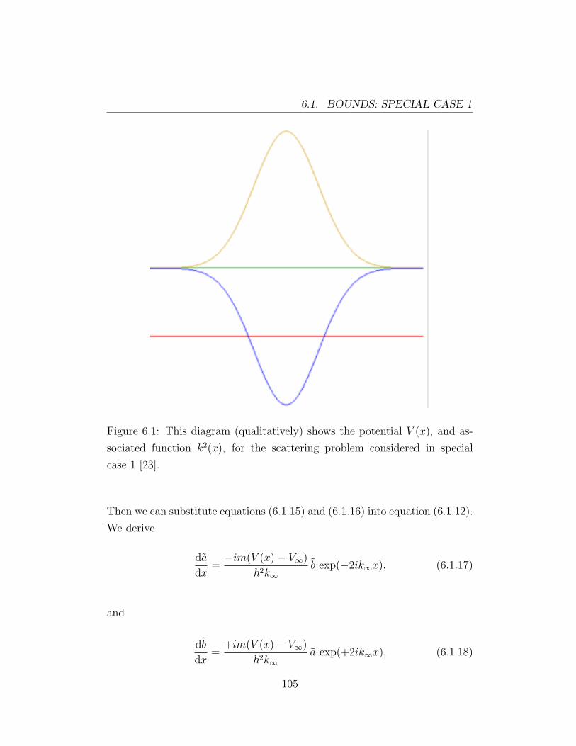
6.1. BOUNDS: SPECIAL CASE 1
Figure 6.1: This diagram (qualitatively) shows the potential V (x), and as-
sociated function k2(x), for the scattering problem considered in special
case 1 [23].
Then we can substitute equations (6.1.15) and (6.1.16) into equation (6.1.12).
We derive
da
dx=−im(V (x)− V∞)
~2k∞b exp(−2ik∞x), (6.1.17)
and
db
dx=
+im(V (x)− V∞)
~2k∞a exp(+2ik∞x), (6.1.18)
105

CHAPTER 6. BOUNDS: SPECIAL CASES
respectively. This representation simplifies some of the results, for instance[α β∗
β α∗
]= E(∞,−∞),
= P exp
(−im~2k∞
∫ ∞−∞
(V (x)− V∞)
[0 e−2ik∞x
−e+2ik∞x 0
]dx
).
(6.1.19)
Also note that
α = α exp
[+
im
~2k∞
∫ +∞
−∞(V (y)− V∞) dy
], (6.1.20)
β = β exp
[− im
~2k∞
∫ +∞
−∞(V (y)− V∞) dy
]. (6.1.21)
This can be used as the basis of an approximation scheme for β. Suppose
that for all x we have |b(x)| 1, so that |a(x)| ≈ 1. Then
db
dx≈ +im(V (x)− V∞)
~2k∞exp(+2ik∞x). (6.1.22)
This may be immediately integrated to yield
β ≈∫
+im(V (x)− V∞)
~2k∞exp(+2ik∞x) dx. (6.1.23)
This is immediately recognizable as the (first) Born approximation. If we
instead work in terms of the original definition β we obtain a slightly different
approximation
β ≈ +im
~2k∞exp
[+
im
~2k∞
∫ +∞
−∞(V (x)− V∞) dx
]×
∫ +∞
−∞(V (x)− V∞) exp(+2ik∞x) exp
[− im
~2k∞
∫ x
−∞(V (x)− V∞) dy
]dx.
(6.1.24)
This is one form of the distorted Born wave approximation.
106

6.2. BOUNDS: SPECIAL CASE 2
Definition (The Born approximation in scattering theory):
The Born approximation consists of taking the unperturbed incident
field, in place of the total field, as the driving field at each point in
the scatterer. It is the perturbation technique most commonly applied
to scattering by an extended body. It is a good approximation if the
scattered field is small, compared to the incident field, everywhere
inside the scatterer [27].
For our purposes, the Born approximation is a good approximation
whenever the “reflected wave”, characterized in our notation by b(x),
is small everywhere, |b(x)| 1. (This is a stronger statement than
merely saying |β| 1.) Similarly, one requires the reflection ampli-
tude to satisfy |r| 1.
In brief, the analysis of this chapter has so far collected together a large
number of results that otherwise appear quite unrelated. By taking further
specific cases of these bounds, and related results, it is possible to reproduce
many analytically known results, such as those for delta-function potentials,
double-delta-function potentials, square wells, and sech2 potentials, as dis-
cussed later in this chapter.
6.2 Bounds: special case 2
Having developed a good understanding of the bounds for special case 1,
now we reconsider the bounds for special case 2 in [88]: Suppose now we
take k(x) = ϕ′(x) 6= 0 and again set χ = 0. This implies that we are
choosing our auxiliary function so that we use the WKB approximation for
the true wavefunction as a “basis” for calculating the Bogoliubov coefficients.
This choice is perfectly capable of dealing with the case V+∞ 6= V−∞, but
by reason of the assumed reality of ϕ is limited to considering scattering over
107

CHAPTER 6. BOUNDS: SPECIAL CASES
the potential barrier. (This is the special case implicit in a different context
in [55]). The evolution equations again simplify tremendously.
When we substitute k(x) = ϕ′(x) and χ = 0 into equation (4.5.55) and
equation (4.5.56), we obtain:
da
dx= +
1
2ϕ′
ϕ′′ b exp(−2iϕ)
, (6.2.1)
db
dx= +
1
2ϕ′
ϕ′′ a exp(+2iϕ)
. (6.2.2)
This form of the evolution equations can be related to the qualitative discus-
sion of scattering “over a potential barrier” presented by Migdal [57, 58]. For
this choice of auxiliary functions we consider the equation (6.1.1) to derive
ϑ[k(x), ϕ(x), χ] =
√(ϕ′′)2
2|ϕ′|=|ϕ′′|2|ϕ′|
=|k′|2|k|
, (6.2.3)
ϑ→ |ϕ′′|2|ϕ′|
=|k′|2|k|
, (6.2.4)
and the bounds become
T ≥ sech2
(1
2
∫ +∞
−∞
|k′||k|
dx
), (6.2.5)
and
R ≤ tanh2
(1
2
∫ +∞
−∞
|k′||k|
dx
). (6.2.6)
The relevant transfer matrix is now
E(xf , xi) = P exp
(1
2
∫ xf
xi
ϕ′′
ϕ′
[0 e−2iϕ
−e+2iϕ 0
]dx
). (6.2.7)
The Bogoliubov coefficients are now[α β∗
β α∗
]= E(∞,−∞) = P exp
(∫ ∞−∞
ϕ′′
ϕ′
[0 e−2iϕ
−e+2iϕ 0
]dx
).
(6.2.8)
108

6.3. REFLECTION ABOVE THE BARRIER
6.3 Reflection above the barrier
The system (6.2.1)-(6.2.2) can also be used as the basis of an approximation
scheme for β. Suppose that for all x we have |b(x)| 1, so that |a(x)| ≈ 1.
Thendb
dx≈ ϕ′′
2ϕ′exp(+2iϕ). (6.3.1)
This may be immediately integrated to yield
β ≈ 1
2
∫ +∞
−∞
ϕ′′(x)
ϕ′(x)exp(+2iϕ) dx. (6.3.2)
Or the equivalent
β ≈ 1
2
∫ +∞
−∞
k′(x)
k(x)exp
(+ 2i
∫ x
−∞k(y) dy
)dx. (6.3.3)
This result serves to clarify the otherwise quite mysterious discussion of so-
called “reflection above the barrier” given by Migdal [57, 58]. Even though
the WKB wavefunctions are buried in the representation of the wavefunction
underlying the analysis leading to this approximation, the validity of this
result for |β| does not require validity of the WKB approximation.
If the shifted potential, V − V∞, is “small” then we can recover the
Born approximation in the usual manner. In that case k′ ≡ mV ′/(~2k) ≈mV ′/(~2k∞), while exp(2i
∫k) ≈ exp(2ik∞x). A single integration by parts
then yields
β ≈ −i m
~2k∞
∫ +∞
−∞(V (x)− V∞) exp(+2ik∞x) dx. (6.3.4)
This is now equivalent to the first Born approximation, in this particular
context.
6.4 Under the barrier?
What goes wrong when we try to extend this analysis into the classically for-
bidden region? Analytically continuing the system (6.2.1)–(6.2.2) is trivial,
109

CHAPTER 6. BOUNDS: SPECIAL CASES
Quantum effect: The reflection probability R = |r|2 is a function of
the energy of the incoming particles. It can always in principle be eval-
uated by numerically integrating the Schrodinger equation for different
values of kinetic energy, E and potential energy, V (x). (However, the
central idea of this thesis is to see just how much we can do ana-
lytically, without resorting to numerical integration.) Furthermore,
“quantum effects”, such as over-barrier reflection and under-barrier
transmission, are dominated by regions of the potential where the
naive semiclassical treatment fails. Due to tunneling, the reflection
probabilities at energies above the barrier are larger than zero, and
the under-barrier reflection probabilities are smaller than one [28].
replace
k2 =2m[E − V (x)]
~2=
2m[V (x)− E]
~2i2, (6.4.1)
therefore
k =
√2m[V (x)− E]
~i, (6.4.2)
and (as required)
ϕ′(x) = k → iκ = i√
2m(V − E)/~ . (6.4.3)
Now let
κ =√
2m(V − E)/~, (6.4.4)
and write
ϕ(x) = ϕtp + i
∫ x
tp
κ(y) dy . (6.4.5)
We will now use these results to re-analyze the Shabat–Zakharov system.
110
6.4. UNDER THE BARRIER?
Substitute the two above equations into equation (6.2.1), we obtain
da
dx= +
1
2ϕ′
ϕ′′ b exp(−2iϕ)
,
= +κ′
2κb exp(−2iϕ),
= +κ′
2κb exp
(− 2i
(ϕtp + i
∫ x
tp
κ(y) dy
)),
= +κ′
2κb exp(−2iϕtp) exp
(+ 2
∫ x
tp
κ(y) dy
),
= +κ′
2κb exp(−2iϕtp) exp
(+ 2
∫κ
). (6.4.6)
Similarly to the equation (6.2.2), we obtain
db
dx= +
1
2ϕ′
ϕ′′ a exp(+2iϕ)
,
= +κ′
2κa exp(+2iϕ),
= +κ′
2κa exp
(+ 2i
(ϕtp + i
∫ x
tp
κ(y) dy
)),
= +κ′
2κa exp(+2iϕtp) exp
(− 2
∫ x
tp
κ(y) dy
),
= +κ′
2κa exp(+2iϕtp) exp
(− 2
∫κ
). (6.4.7)
Thus we are now violating our previous condition that ϕ be real, though
we still require ϕ′ 6= 0. This is a perfectly good Shabat–Zakharov system
that works in the forbidden region. But you cannot now use this to derive
bounds on the transmission coefficient. The fly in the ointment resides in the
fact that the formula for the probability current is modified, and that in the
forbidden region the probability current is
J = Im
ψ∗
dψ
dx
= Imab∗ exp(+2iϕtp). (6.4.8)
We can derive the above equation by combining
J = Im
ψ∗
dψ
dx
, (6.4.9)
111

CHAPTER 6. BOUNDS: SPECIAL CASES
and
J = |a|2 − |b|2. (6.4.10)
For a properly normalized flux in the allowed region (|a|2−|b|2 = 1), we have
in the forbidden region
Im ab∗ exp(+2iϕtp) = 1. (6.4.11)
While this does imply 2|a||b| > 1, the inequality is unfortunately in the wrong
direction to be useful for placing bounds on the transmission coefficient. It
is for this reason that we have gone to the trouble of keeping track of the
more general gauge condition represented by χ — in the hope that we can
use this to explore under the barrier.
A good rigorous bound (not just a WKB approximation) on transmission
under the barrier would be very useful. The best we have been able to
do along these lines is presented in chapter 10 discussing the Miller–Good
transformation.
6.5 Special case 2-a
Suppose now that V (x) is continuous and monotonic increasing or decreasing,
varying from V−∞ = V (−∞) to V+∞ = V (+∞).
Suppose E ≥ maxV−∞, V+∞ so there is no classical turning point. Then∫ +∞
−∞
|k′||k|
dx =
∣∣∣∣ ln(k+∞
k−∞
)∣∣∣∣, (6.5.1)
and the transmission and reflection probabilities satisfy
T ≥ 4k+∞k−∞(k+∞ + k−∞)2
, (6.5.2)
and
R ≤ (k+∞ − k−∞)2
(k+∞ + k−∞)2. (6.5.3)
112

6.5. SPECIAL CASE 2-A
Figure 6.2: Sharp corners are guaranteed to maximize reflection, and abrupt
transitions are guaranteed to maximize particle production [23].
Calculation: We consider
ϑ[k(x), ϕ(x), χ] =1
2
|k′||k|
, (6.5.4)
and the bounds become
T ≥ sech2
(∫ +∞
−∞
1
2
|k′||k|
dx
)= sech2
(1
2
∣∣∣∣ ln(k+∞
k−∞
)∣∣∣∣), (6.5.5)
≥ sech2
(1
2
∣∣∣∣ ln(k+∞
k−∞
)∣∣∣∣).Remembering that
sech(x) =2
exp(+x) + exp(−x), (6.5.6)
113

CHAPTER 6. BOUNDS: SPECIAL CASES
and noting
exp
(1
2
∣∣∣∣ ln(k+∞/k−∞)
∣∣∣∣) = max
[√k+∞
k−∞,
√k−∞k+∞
], (6.5.7)
we see that
sech
(1
2
∣∣∣∣ ln(k+∞
k−∞
)∣∣∣∣) =2√k+∞k−∞
(k+∞ + k−∞). (6.5.8)
Therefore
sech2
(1
2
∣∣∣∣ ln(k+∞
k−∞
)∣∣∣∣) =4k+∞k−∞
(k+∞ + k−∞)2, (6.5.9)
so we obtain
T ≥ 4k+∞k−∞(k+∞ + k−∞)2
, (6.5.10)
as required. We now consider
R ≤ tanh2
(1
2
∫ +∞
−∞
|k′||k|
dx
), (6.5.11)
≤ tanh2
(1
2
∣∣∣∣ ln(k+∞
k−∞
)∣∣∣∣),≤ (k+∞ − k−∞)2
(k+∞ + k−∞)2,
as required. These bounds are instantly understandable as the exact analytic
results for a step-function potential [37, 43, 44, 88], and the result asserts
that for arbitrary smooth monotonic potentials the step function provides
upper and lower bounds on the exact result. If we are interested in physical
situations such as a time-dependent refractive index [60, 61], or particle pro-
duction due to the expansion of the universe [63], this technique shows that
sudden changes in refractive index or size of the universe provide a strict
upper bound on particle production.
6.6 Special case 2-b
Suppose now that V (x) has a single unique extremum (either a peak or
a valley). Provided that E ≥ maxV−∞, Vextremum, V+∞ so that there is no
114

6.6. SPECIAL CASE 2-B
classical turning point, then k(x) moves monotonically from k−∞ to kextremum
and then back to k+∞. Under these circumstances we consider∫ +∞
−∞
|k′|k
dx =
∣∣∣∣ ln [kextremum
k−∞
]∣∣∣∣+
∣∣∣∣ ln [kextremum
k+∞
]∣∣∣∣ , (6.6.1)
=
∣∣∣∣ ln [kextremum
k−∞× kextremum
k+∞
]∣∣∣∣ , (6.6.2)
=
∣∣∣∣ ln [k2extremum
k−∞k+∞
]∣∣∣∣, (6.6.3)
as required.
The bound (4.5.18) implies
|α| ≤ cosh
∣∣∣∣ ln [ kextremum√k−∞k+∞
]∣∣∣∣ , (6.6.4)
and which yields
|β| ≤ sinh
∣∣∣∣ ln [ kextremum√k−∞k+∞
]∣∣∣∣. (6.6.5)
Numerous generalizations of these formulae are possible. For example, at the
cost of a little extra notation, we also already have enough information to
provide a bound on an asymmetric barrier or asymmetric well, as long as it
has only a single extremum (maximum or minimum) we apply the previous
equations to derive
|α| ≤ k2extremum + k+∞k−∞
2kextremum
√k+∞k−∞
, (6.6.6)
and
|β| ≤ |k2extremum − k+∞k−∞|
2kextremum
√k+∞k−∞
. (6.6.7)
Calculation:
|α| ≤ cosh
∣∣∣∣ ln [ kextremum√k−∞k+∞
]∣∣∣∣,=
exp
(+
∣∣∣∣ ln [ kextremum√k−∞k+∞
]∣∣∣∣)+ exp
(−∣∣∣∣ ln [ kextremum√
k−∞k+∞
]∣∣∣∣)2
,
=k2
extremum + k−∞k+∞
2kextremum
√k−∞k+∞
, (6.6.8)
115

CHAPTER 6. BOUNDS: SPECIAL CASES
as required.
In addition, we can derive
|β| ≤ sinh
∣∣∣∣ ln [ kextremum√k−∞k+∞
]∣∣∣∣ ,=
exp
(+
∣∣∣∣ ln [ kextremum√k−∞k+∞
]∣∣∣∣)− exp
(−∣∣∣∣ ln [ kextremum√
k−∞k+∞
]∣∣∣∣)2
,
=|k2
extremum − k−∞k+∞|2kextremum
√k−∞k+∞
, (6.6.9)
as required.
Translated into statements about the transmission and reflection proba-
bilities this becomes
T ≥ 4k+∞k−∞k2extremum
k2extremum + k+∞k−∞2
, (6.6.10)
and
R ≤ k2extremum − k+∞k−∞2
k2extremum + k+∞k−∞2
. (6.6.11)
Calculation:
T ≥ sech2
(∫ +∞
−∞
|k′|2k
dx
)= sech2
(1
2
∣∣∣∣ ln [k2extremum
k−∞k+∞
]∣∣∣∣), (6.6.12)
= sech2
(∣∣∣∣ ln [ kextremum√k−∞k+∞
]∣∣∣∣),=
4k+∞k−∞k2extremum
k2extremum + k+∞k−∞2
.
Also
R ≤ tanh2
(∫ +∞
−∞
|k′|2k
dx
)= tanh2
(∣∣∣∣ ln [ kextremum√k−∞k+∞
]∣∣∣∣). (6.6.13)
But
tanh(x) =(exp(2x)− 1)
(exp(2x) + 1), (6.6.14)
116

6.6. SPECIAL CASE 2-B
therefore
R ≤ tanh2
∣∣∣∣ ln [ kextremum√k−∞k+∞
]∣∣∣∣, (6.6.15)
implying
R ≤ k2extremum − k+∞k−∞2
k2extremum + k+∞k−∞2
, (6.6.16)
as required.
Equivalently
T ≥4(E − Vextremum)
√(E − V+∞)(E − V−∞)
[(E − Vextremum) +√
(E − V+∞)(E − V−∞)]2, (6.6.17)
and
R ≤[(E − Vextremum)−
√(E − V+∞)(E − V−∞)]2
[(E − Vextremum) +√
(E − V+∞)(E − V−∞)]2. (6.6.18)
Calculation: We consider
k±∞ =
√2m (E − V±∞)
~, (6.6.19)
and
kextremum =
√2m (E − Vextremum)
~. (6.6.20)
we substitute the above equations into equation (6.6.10) to derive equation
(6.6.17). Moreover, we substitute the above equation into equation (6.6.11)
to derive equation (6.6.18).
This can be compared, for example, with known analytic results for the
asymmetric square well. To be more specific, if in addition V (−∞) =
V (+∞) = V∞, so that k−∞ = k+∞ = k∞, then we have
|α| ≤ k2extremum + k2
∞2kextremumk∞
, (6.6.21)
and
|β| ≤ |k2extremum − k2
∞|2kextremumk∞
. (6.6.22)
117
CHAPTER 6. BOUNDS: SPECIAL CASES
Translated into statements about the transmission and reflection probabili-
ties this becomes
T ≥ (E − V∞)(E − Vextremum)
(E − V∞)(E − Vextremum) + 14(Vextremum − V∞)2
, (6.6.23)
and
R ≤14(Vextremum − V∞)2
(E − V∞)(E − Vextremum) + 14(Vextremum − V∞)2
. (6.6.24)
Equivalently
T ≥ 1− (Vextremum − V∞)2
(2E − Vextremum − V∞)2, (6.6.25)
and
R ≤ (Vextremum − V∞)2
(2E − Vextremum − V∞)2. (6.6.26)
For low energies, these results are weaker than the bounds derived under
special case 1, (6.1.6, 6.1.7) and (6.1.8, 6.1.9), but have the advantage of
requiring more selective information about the potential. For high energies,
E ~2(Vextremum − V∞)2
2m( ∫ +∞−∞ |V (x)− V∞| dx
)2 , (6.6.27)
the present result (when it is applicable) leads to tighter bounds on the
transmission and reflection coefficients.
6.7 Special case 2-c
Suppose now that V (x) has a number of extrema, (both peaks and val-
leys). We allow V (+∞) 6= V (−∞), but demand that for all extrema E ≥maxV−∞, V+∞, V
iextremum so that there is no classical turning point.
For definiteness, suppose the ordering is: −∞→ peak→ valley . . . valley
→ peak → +∞. Then∫ +∞
−∞
|k′|k
dx =
∣∣∣∣∣ ln[k1
peak
k−∞
]∣∣∣∣∣+
∣∣∣∣∣ ln[k1
valley
k1peak
]∣∣∣∣∣+ . . .
· · ·+
∣∣∣∣∣ ln[knpeak
kn−1valley
]∣∣∣∣∣+
∣∣∣∣∣ ln[k+∞
knpeak
]∣∣∣∣∣. (6.7.1)
118

6.7. SPECIAL CASE 2-C
Defining
Πp(k) ≡∏
peaks
kipeak, (6.7.2)
Πv(k) ≡∏
valley
kivalley, (6.7.3)
Πe(k) ≡∏
extrema
kiextremum = Πp(k) Πv(k), (6.7.4)
we see ∫ +∞
−∞
|k′|k
dx =
∣∣∣∣∣ ln[
Π2p(k)
k−∞k+∞Π2v(k)
]∣∣∣∣∣. (6.7.5)
This bounds the Bogoliubov coefficients as
|α| ≤k−∞k+∞Π2
v(k) + Π2p(k)
2√k+∞k−∞Πe(k)
, (6.7.6)
and
|β| ≤|k−∞k+∞Π2
v(k)− Π2p(k)|
2√k+∞k−∞Πe(k)
. (6.7.7)
Then the transmission and reflection probabilities satisfy
T ≥ 4k+∞k−∞Π2e(k)
Π2p(k) + k+∞k−∞Π2
v(k)2 , (6.7.8)
and
R ≤
Π2p(k)− k+∞k−∞Π2
v(k)2
Π2p(k) + k+∞k−∞Π2
v(k)2 . (6.7.9)
In these formulae, peaks and valleys can be interchanged in the obvious way,
and by letting the initial or final peak sink down to V±∞ as appropriate we
obtain bounds for sequences such as: −∞→ valley→ peak . . . valley→ peak
→ +∞, or: −∞ → peak → valley . . . peak → valley → +∞. In the case
of one or zero extrema these formulae reduce to the previously given results.
[Equations (6.6.10)–(6.6.11).] Further modifications of these formulae are
still possible, the cost is that more specific assumptions are needed to derive
more specific results.
119

CHAPTER 6. BOUNDS: SPECIAL CASES
6.8 Bounds: Special case 3
In the following we will consider the bounds in special case 3. In particular,
the most outstanding features of this case is:
Let χ = 0, k0 > 0 and pick
ϕ′ =√
maxk2(x), k20, (6.8.1)
with x±0 defined by k2(x±0 ) = k20. Then we have
ϑ =
1
2
|k′||k|
k2 > k20;
1
2
k20 − k2
k0
k2 < k20.
(6.8.2)
Note that there are step function discontinuities at x±0 , but no delta-function
contribution. It now follows that∮ϑ =
1
2ln
[k−∞k0
]+
1
2k0
∫k2<k2
0
[k20 − k2] dx+
1
2ln
[k+∞
k0
], (6.8.3)
that is ∮ϑ =
1
2ln
[k−∞k+∞
k20
]+
1
2k0
∫k2<k2
0
[k20 − k2] dx. (6.8.4)
Consider ∫k2<0
(−k2) dx =
∫F
κ2 dx, (6.8.5)
so
1
2k0
∫k2<k2
0
[k20 − k2] dx ≤ 1
2k0
(∫F
κ2 dx+ k20 Lk2<k2
0
),
≤ 1
2k0
∫κ2 dx+
1
2k0 Lk2<k2
0. (6.8.6)
So collecting terms we have∮ϑ ≤ 1
2ln
[k−∞k+∞
k20
]+
1
2k0
∫κ2 dx+
1
2k0 Lk2<k2
0. (6.8.7)
120

6.9. BOUNDS: SPECIAL CASE 4
Now note
T ≥ sech2
∮ϑ,
≥ sech2
(1
2ln
[k−∞k+∞
k20
]+
1
2k0
∫κ2 dx+
1
2k0 Lk2<k2
0
), (6.8.8)
so that
T ≥ 4√k−∞k+∞
k0
exp(B(x)) +k0√
k−∞k+∞exp(−B(x))
2, (6.8.9)
where
B(x) =1
2k0
∫κ2 dx+
1
2k0 Lk2<k2
0, (6.8.10)
when k0 is still an adjustable parametric, though we definitely need 0 < k0 <
mink+∞, k−∞.
6.9 Bounds: Special case 4
For the fourth special case we want to derive something that looks simi-
lar to the WKB approximation, but is a strict bound instead of being an
(uncontrolled) estimate.
Choose χ = 0, k0 > 0 and pick
ϕ′ =√
max|k2(x)|, k20. (6.9.1)
Even for a potential with only a single hump there are now five regions to
analyze, the two allowed regions, the forbidden region, and two transition
regions enclosing the two the classical turning points. As usual we shall
define our notation so that in the forbidden region:
κ2(x) = −k2(x); κ > 0. (6.9.2)
In the two allowed regions
ϑ =1
2
|k′||k|
; k2 > k20. (6.9.3)
121

CHAPTER 6. BOUNDS: SPECIAL CASES
In the two transition regions
ϑ =1
2
k20 − k2
k0
; −k20 < k2 < k2
0. (6.9.4)
Finally in the forbidden region
ϑ =1
2
√(κ′)2
κ2+ κ2; k2 < −k2
0. (6.9.5)
So in the forbidden region by the triangle inequality
ϑ ≤ 1
2
(|κ′|κ
+ κ
); k2 < −k2
0. (6.9.6)
Collecting these∮ϑ ≤ 1
2ln
[k−∞k0
]+
1
2k0
∫ k2decreasing
k20>k
2>−k20
[k20 − k2] dx
+1
2ln
[κextremum
k0
]+
1
2
∫κ2>k2
0
κ(x)dx+1
2ln
[κextremum
k0
]+
1
2k0
∫ k2inclreasing
−k20<k
2<k20
[k20 − k2] dx+
1
2ln
[k+∞
k0
]. (6.9.7)
Now in each of the transition regions
0 ≤ k20 − k2 ≤ 2k2
0, (6.9.8)
so ∫−k2
0<k2<k2
0
[k20 − k2] dx ≤ 2k2
0
∫−k2
0<k2<k2
0
1 dx, (6.9.9)
= 2k20 L−k2
0<k2<k2
0. (6.9.10)
Here L−k20<k
2<k20
is the combined length of the transition regions −k20 < k2 <
k20. That is, the integral coming from each transition region is bounded (up
to a constant) by the physical width of that transition region. Furthermore
in the forbidden region∫κ2>k2
0
κ(x) dx ≤∫κ2>0
κ(x) dx, (6.9.11)
122

6.9. BOUNDS: SPECIAL CASE 4
so collecting terms we have∮ϑ ≤ 1
2ln
[k−∞k+∞κ
2extremum
k40
]+ k0 L−k2
0<k2<k2
0+
1
2
∫κ2>0
κ(x) dx, (6.9.12)
where L now denotes the combined total width of the two transition regions.
Now note
T ≥ sech2
∮ϑ ≥ exp
(− 2
∮ϑ
), (6.9.13)
so that
T ≥ k40
k−∞k+∞κ2extremum
exp[−2k0 L(k0)] exp
[−∫κ2>0
κ(x)dx
]. (6.9.14)
The bound is considerably weaker than could have been derived by making
more restrictive hypotheses, but has the advantage of elegance and looking
very similar to the WKB bound. Note the key requirements: We must be
dealing with a single-hump potential, and k0 must be in the range
0 < k0 < mink−∞, k+∞, κextremum. (6.9.15)
The parameter k0 is otherwise arbitrary, and so can be chosen to maximize
the prefactor.
One thing we could do is to choose a different value of k0 at each tran-
sition, call them k1 and k2, and repeat the analysis keeping careful track of
the κ integration near the turning points. Then∮ϑ ≤ 1
2ln
[k−∞k+∞κ
2extremum
k21 k
22
]+
1
2k1
∫−k2
1<k2<k2
1
[k21 − k2] dx− 1
2
∫k21>κ
2>0
κ(x) dx
+1
2k2
∫−k2
2<k2<k2
2
[k22 − k2] dx− 1
2
∫k22>κ
2>0
κ(x) dx
+1
2
∫κ2>0
κ(x) dx.
So far this is a rigorous bound; now we are going to adopt a linear approxi-
mation near the turning points, so that near the first turning point
k2(x) ≈ s1(x− x1), (6.9.16)
123

CHAPTER 6. BOUNDS: SPECIAL CASES
with k(x) reaching the values ±k21 at the positions x = x1±k2
1/s1. Therefore
L1 = 2k21/s1. Then∫
−k21<k
2<k21
[k21 − k2] dx ≈
∫ x1+k21/s1
x1−k21/s1
[k21 − s1(x− x1)] dx =
2k41
s1
. (6.9.17)
Similarly∫k21>κ
2>0
κ(x)dx ≈∫ x1+k2
1/s1
x1
√s1(x− x1) dx =
2
3
k31
s1
, (6.9.18)
so that combining, and assuming the linear approximation is a good one∮ϑ ≤ 1
2ln
[k−∞k+∞κ
2extremum
k21k
22
]+
2
3
k31
s1
+2
3
k32
s2
+1
2
∫κ2>0
κ(x) dx. (6.9.19)
Extremize with respect to k1, then
− 1
k1
+2k2
1
s1
= 0; so k31 =
1
2s1, (6.9.20)
and similarly for k2, then∮ϑ ≤ 1
2ln
[k−∞k+∞κ
2extremum
((1/2)s1)2/3 ((1/2)s2)2/3
]+
2
3+
1
2
∫κ2>0
κ(x) dx, (6.9.21)
and hence
T ≥ ((1/2)s1)2/3 ((1/2)s2)2/3
k−∞k+∞κ2extremum
exp[−4/3] exp
[−∫κ2>0
κ(x) dx
]. (6.9.22)
Although such results are certainly a major advance in our standing of the
rigorous bounds, this particular bound is not 100% rigorous due to the linear
approximation. This suggests that further exploration of these ideas, with a
view to obtaining a 100% rigorous bound, might be profitable.
6.10 Bounds: Future directions
From the general definition
ϑ[k(x), ϕ(x), χ(x)] ≡
√(ϕ′′ + 2χϕ′)2 + [k2(x) + χ2 + χ′ − (ϕ′)2]2
2|ϕ′|, (6.10.1)
124

6.11. DISCUSSION
and the bound
T ≥ sech2
[ ∮ϑ dx
], (6.10.2)
there are many other special cases you could in principle derive. The possi-
bilities seem endless and the art is in finding something useful.
6.11 Discussion
In this chapter we dealt with some specific cases of the general bounds and
developed a number of interesting specializations. In addition, we collected
together a large number of results that otherwise appeared quite unrelated,
including reflection above and below the barrier. The special case bounds
were divided into five topics: special cases 1–4, and “future directions”. In
addition, all special cases were chosen for their directness and simplicity.
Furthermore, special case 1, as presented in equations (6.1.6)–(6.1.7) and
(6.1.8)–(6.1.9), has the advantage that it applies to both scattering over the
barrier and under the barrier. On the other hand, special case 2, as presented
in equations (6.2.5)–(6.2.6) and their specializations, applies only to scatter-
ing over the barrier but has the advantage of being much more selective in
how much information is needed concerning the scattering potential.
125

CHAPTER 6. BOUNDS: SPECIAL CASES
126

Chapter 7
Parametric oscillations
7.1 Introduction
In this chapter we shall present the basic concept of a “parametric oscilla-
tor”. This is a simple harmonic oscillator whose parameters (its resonance
frequency ω and damping time β) vary in time. The other interesting way of
understanding a parametric oscillator is that it is a device that oscillates when
one of its “parameters” (a physical entity, like capacitance) is changed [119].
We shall re-cast and represent the general bounds in terms of the spe-
cific mathematical structure of parametric oscillations. This time-dependent
problem is closely related to the spatial properties of the time-independent
Schrodinger equation.
Although the discussion so far has been presented in terms of the spatial
properties of the time-independent Schrodinger equation, the mathematical
structure of parametrically excited oscillations is identical, needing only a few
minor translations to be brought into the current form. For a parametrically
excited oscillator we have
d2φ
dt2= ω(t)2 φ. (7.1.1)
Just map t → x, ω(t) → k(x), and φ → ψ. In the general analysis of
127

CHAPTER 7. PARAMETRIC OSCILLATIONS
equation (6.1.1) the quantity ϑ should be replaced by
ϑ[ϕ(t), ω(t)] ≡
√(ϕ′′)2 + [ω2 − (ϕ′)2]2
2|ϕ′|. (7.1.2)
This is often written as
ϑ[ϕ(t), ω(t)] ≡
√(ϕ)2 + [ω2 − (ϕ)2]2
2|ϕ|, (7.1.3)
but this is purely a convention, a change in notation. (Physicists typically
use dots for time derivatives and primes for space derivatives.) The analysis
then parallels that of the Schrodinger equation. Some key results are given
below.
7.2 Special case 1
If ω(−∞) = ω0 = ω(+∞) 6= 0, then by choosing the auxiliary function to be
ϕ = ω0 t we can use equations (5.3.7)–(5.3.14) to deduce
|α| ≤ cosh
(1
2ω0
∫ +∞
−∞|ω2(t)− ω2
0| dt), (7.2.1)
and
|β| ≤ sinh
(1
2ω0
∫ +∞
−∞|ω2(t)− ω2
0| dt). (7.2.2)
Calculation: We now consider
|α| ≤ cosh
(∫ +∞
−∞ϑ[ϕ(t), ω(t)] dt
). (7.2.3)
We substitute equation (7.1.2) into equation (7.2.3), now we derive
|α| ≤ cosh
∫ +∞
−∞
√(ϕ′′)2 + [ω2 − (ϕ′)2]2
2|ϕ′|dt
. (7.2.4)
128
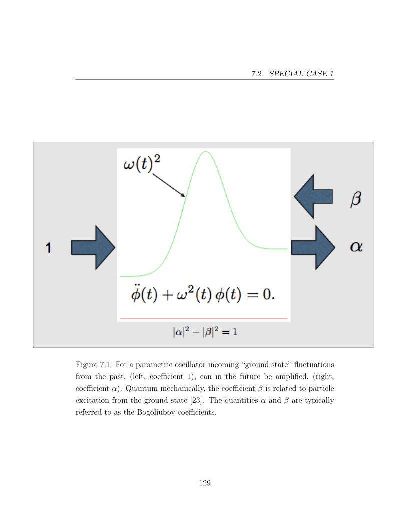
7.2. SPECIAL CASE 1
Figure 7.1: For a parametric oscillator incoming “ground state” fluctuations
from the past, (left, coefficient 1), can in the future be amplified, (right,
coefficient α). Quantum mechanically, the coefficient β is related to particle
excitation from the ground state [23]. The quantities α and β are typically
referred to as the Bogoliubov coefficients.
129

CHAPTER 7. PARAMETRIC OSCILLATIONS
Furthermore, under the stated assumptions we can simplify the above integral
to derive
|α| ≤ cosh
(1
2ω0
∫ +∞
−∞|ω2(t)− ω2
0| dt), (7.2.5)
which automatically implies
|β| ≤ sinh
(1
2ω0
∫ +∞
−∞|ω2(t)− ω2
0| dt), (7.2.6)
as required.
7.3 Special case 2
If ω(−∞) and ω(+∞) 6= 0 are both finite so that suitable asymptotic states
exist, and assuming ω2(t) ≥ 0 so that the frequency is always positive, then
applying equations (6.2.5)–(6.2.6) to the case of parametric resonance yields
|α| ≤ cosh
∣∣∣∣ ∫ +∞
−∞
1
2
|ω′(t)||ω(t)|
dt
∣∣∣∣ , (7.3.1)
and
|β| ≤ sinh
∣∣∣∣ ∫ +∞
−∞
1
2
|ω′(t)||ω(t)|
dt
∣∣∣∣ . (7.3.2)
7.4 Special case 2-a
Suppose now that ω2(t) is positive semidefinite, continuous, and monotonic
increasing or decreasing, varying from ω−∞ = ω(−∞) 6= 0 to some distinct
value ω+∞ = ω(+∞) 6= 0. The Bogoliubov coefficients satisfy
|α| ≤ ω−∞ + ω+∞
2√ω−∞ω+∞
, (7.4.1)
and
|β| ≤ |ω−∞ − ω+∞|2√ω−∞ω+∞
. (7.4.2)
130

7.5. SPECIAL CASE 2-B
Calculation: We now consider
|α| ≤ cosh
∣∣∣∣ ∫ +∞
−∞
1
2
|ω′(t)||ω(t)|
dt
∣∣∣∣ , (7.4.3)
≤ cosh
∣∣∣∣12 ln
(ω+∞
ω−∞
)∣∣∣∣ ,≤ ω−∞ + ω+∞
2√ω−∞ω+∞
,
as required. Similarly
|β| ≤ sinh
∣∣∣∣ ∫ +∞
−∞
1
2
|ω′(t)||ω(t)|
dt
∣∣∣∣ , (7.4.4)
≤ sinh
∣∣∣∣12 ln
(ω+∞
ω−∞
)∣∣∣∣ ,≤ |ω−∞ − ω+∞|
2√ω−∞ω+∞
,
as required.
7.5 Special case 2-b
Under the restriction ω(−∞) = ω0 = ω(+∞) 6= 0, with the additional
constraint that ω(t) has a single unique extremum (either a maximum or a
minimum but not both), and provided that ω2extremum > 0 so that we do not
encounter complex frequencies (no classical turning point), the Bogoliubov
coefficients satisfy
|α| ≤ ω20 + ω2
extremum
2ω0ωextremum
, (7.5.1)
and
|β| ≤ |ω20 − ω2
extremum|2ω0ωextremum
. (7.5.2)
131

CHAPTER 7. PARAMETRIC OSCILLATIONS
Calculation: To prove the above equations, we consider∫ +∞
−∞
|ω′|ω
dx =
∣∣∣∣ ln [ωextremum
ω−∞
]∣∣∣∣+
∣∣∣∣ ln [ωextremum
ω+∞
]∣∣∣∣ , (7.5.3)
=
∣∣∣∣ ln [ω2extremum
ω−∞ω+∞
]∣∣∣∣ , (7.5.4)
=
∣∣∣∣ ln [ω2extremum
ω20
]∣∣∣∣.This implies
|α| ≤ cosh
∣∣∣∣12 ln
[ω2
extremum
ω20
]∣∣∣∣ , (7.5.5)
≤ cosh
∣∣∣∣ ln [ωextremum
ω0
]∣∣∣∣ ,≤ ω2
0 + ω2extremum
2ω0ωextremum
.
Furthermore,
|β| ≤ sinh
∣∣∣∣12 ln
[ω2
extremum
ω20
]∣∣∣∣ , (7.5.6)
≤ sinh
∣∣∣∣ ln [ωextremum
ω0
]∣∣∣∣ ,≤ |ω2
extremum − ω20|
2ω0ωextremum
.
Suppose now that ω2(t) has a single unique extremum (either a peak or a
valley), but that we allow the two asymptotic frequencies to differ ω(+∞) 6=ω(−∞), and suppose further that ω2(t) > 0 so that there is no classical
turning point. The Bogoliubov coefficients satisfy
|α| ≤ ω−∞ω+∞ + ω2extremum
2√ω−∞ω+∞ωextremum
, (7.5.7)
and
|β| ≤ |ω−∞ω+∞ − ω2extremum|
2√ω−∞ω+∞ωextremum
. (7.5.8)
132

7.6. SPECIAL CASE 2-C
Calculation: We now show how to derive the above equations: For the
moment we shall consider
|α| ≤ cosh
∣∣∣∣ ln [ ωextremum√ω−∞ω+∞
]∣∣∣∣ , (7.5.9)
≤ ω2extremum + ω−∞ω+∞
2√ω−∞ω+∞ωextremum
.
But this now yields
|β| ≤ |ω2extremum − ω−∞ω+∞|
2√ω−∞ω+∞ωextremum
, (7.5.10)
as required.
7.6 Special case 2-c
Suppose now that ω(t) has a number of extrema (both peaks and valleys).
We allow ω(+∞) 6= ω(−∞), but demand that for all extrema ωiextremum > 0
so that there is no classical turning point.
For definiteness, suppose the ordering is: −∞→ peak→ valley . . . valley
→ peak → +∞. Define
Πp(ω) ≡∏
peaks
ωipeak, (7.6.1)
Πv(ω) ≡∏
valleys
ωivalley, (7.6.2)
Πe(ω) ≡∏
extrema
ωiextremum. (7.6.3)
The Bogoliubov coefficients satisfy
|α| ≤ω−∞ω+∞Π2
v(ω) + Π2p(ω)
√ω+∞ω−∞Πe(ω)
, (7.6.4)
and
|β| ≤|ω−∞ω+∞Π2
v(ω)− Π2p(ω)|
√ω+∞ω−∞Πe(ω)
. (7.6.5)
133

CHAPTER 7. PARAMETRIC OSCILLATIONS
In these formulae, peaks and valleys can be interchanged in the obvious way,
and by letting the initial or final peak sink down to ω±∞ as appropriate we
obtain bounds for sequences such as: −∞ → valley → peak . . . valley →peak → +∞, or: −∞ → peak → valley . . . peak → valley → +∞. In the
case of one or zero extrema these formulae reduce to the previously given
results.
Again, further specializations of these formulae are still possible. As
always there is a trade-off between the strength of the result and its generality.
Calculation: We see∫ +∞
−∞
|ω′|ω
dt =
∣∣∣∣∣ ln[
Π2p(ω)
ω−∞ω+∞Π2v(ω)
]∣∣∣∣∣. (7.6.6)
The Bogoliubov coefficients in this case are bounded by
|α| ≤ω−∞ω+∞Π2
v(ω) + Π2p(ω)
2√ω+∞ω−∞Πe(ω)
, (7.6.7)
and
|β| ≤|ω−∞ω+∞Π2
v(ω)− Π2p(ω)|
2√ω+∞ω−∞Πe(ω)
. (7.6.8)
7.7 Bounds: Special case 3
We let χ = 0, ω0 > 0, then we can choose
ϕ′ =√
maxω2(t), ω20, (7.7.1)
with t±0 defined by ω2(t±0 ) = ω20. Then we have
ϑ =
1
2
|ω′||ω|
ω2 > ω20;
1
2
ω20 − ω2
ω0
ω2 < ω20.
(7.7.2)
134

7.7. BOUNDS: SPECIAL CASE 3
Note that there are step function discontinuities at t±0 , but no delta-function
contribution. It now follows that∮ϑ =
1
2ln
[ω−∞ω0
]+
1
2ω0
∫ω2<ω2
0
[ω20 − ω2] dt+
1
2ln
[ω+∞
ω0
]. (7.7.3)
That is ∮ϑ =
1
2ln
[ω−∞ω+∞
ω20
]+
1
2ω0
∫ω2<ω2
0
[ω20 − ω2] dt. (7.7.4)
As usual we shall define our notation so that in the forbidden region:∫ω2<0
(−ω2) dt =
∫F
Ω2 dt. (7.7.5)
So1
2ω0
∫ω2<ω2
0
[ω20 − ω2] dt ≤ 1
2ω0
(∫F
Ω2 dt+ ω20 Lω2<ω2
0
),
≤ 1
2ω0
∫Ω2 dt+
1
2ω0 Lω2<ω2
0. (7.7.6)
Collecting terms we have∮ϑ ≤ 1
2ln
[ω−∞ω+∞
ω20
]+
1
2ω0
∫Ω2 dt+
1
2ω0 Lω2<ω2
0, (7.7.7)
and the bound on the Bogoliubov coefficients in this case become
|α| ≤ cosh
(∮ϑ
),
≤√ω−∞ω+∞
2ω0
exp
(1
2ω0
∫Ω2 dt+
1
2ω0 Lω2<ω2
0
)+
ω0
2√ω−∞ω+∞
exp
(− 1
2ω0
∫Ω2 dt− 1
2ω0 Lω2<ω2
0
),
(7.7.8)
and
|β| ≤ sinh
(∮ϑ
),
≤∣∣∣∣√ω−∞ω+∞
2ω0
exp
(1
2ω0
∫Ω2 dt+
1
2ω0 Lω2<ω2
0
)− ω0
2√ω−∞ω+∞
exp
(− 1
2ω0
∫Ω2 dt− 1
2ω0 Lω2<ω2
0
)∣∣∣∣ ,(7.7.9)
135

CHAPTER 7. PARAMETRIC OSCILLATIONS
which gives us our third special case bound. Then the transmission and
reflection probabilities satisfy
T ≥ 4√ω−∞ω+∞
ω0
exp(Z(t)) +ω0√
ω−∞ω+∞exp(−Z(t))
2 , (7.7.10)
and
R ≤ ω−∞ω+∞ exp(Z(t))− ω20 exp(−Z(t))2
ω−∞ω+∞ exp(Z(t)) + ω20 exp(−Z(t))2
, (7.7.11)
where
Z(t) =1
2ω0
∫Ω2 dt+
1
2ω0 Lω2<ω2
0. (7.7.12)
7.8 Discussion
Though the discussion in previous chapters has been presented in terms of
the spatial properties of the time-independent Schrodinger equation, we have
seen in this chapter that the mathematical structure of parametrically excited
oscillations is essentially identical, needing only a few minor translations to
be brought into the current form.
In summary, the bounds presented in this chapter are useful in establish-
ing qualitative analytic properties of parametric oscillators, and as such are
complementary to both explicit numerical investigations and the guidance
extracted from exact analytic solutions.
136

Chapter 8
Bounding the Bogoliubov
coefficients
8.1 Introduction
In this chapter we will again be considering (from a somewhat different point
of view) the problem of finding approximate solutions for wave equations in
general, and quantum mechanical problems in particular. It appears that
as yet relatively little work seems to have been put into the complementary
problem of founding rigorous bounds on the exact solutions. We have in
mind either bounds on parametric amplification and the related quantum
phenomenon of particle production (as encoded in the Bogoliubov coeffi-
cients), or bounds on transmission and reflection coefficients.
In the last section of appendix B, we introduce and discuss the time or-
dering and give some more details of time-ordered exponentials — these are
a very convenient trick for formally solving certain matrix differential equa-
tions. Practising physicists and applied mathematicians will all have seen
the WKB approximation for barrier penetration probability. Unfortunately,
the WKB approximation is an example of an uncontrolled approximation,
and in general we do not know if it is an over-estimate or an under-estimate.
As part of the main work, we modify and improve an approach first
137

CHAPTER 8. BOUNDING THE BOGOLIUBOV COEFFICIENTS
developed in [88]. We shall examine this question by developing a formal
but exact solution for the appropriate second-order linear ODE, in terms of
a time-ordered exponential of 2 × 2 matrices, then relating the Bogoliubov
coefficients to certain invariants of this matrix. By bounding the matrix in
an appropriate manner, we can thereby bound the Bogoliubov coefficients.
8.2 The second-order ODE
We would first like to present “the second-order ODE” techniques developed
in [88], that are applicable to numerous physical situations; situations which
are both extremely interesting and important. Consider the ODE
φ(t) + ω2(t)φ(t) = 0, (8.2.1)
or its equivalent in the space domain [88]
φ′′(x) + k2(x)φ(x) = 0. (8.2.2)
It is easy to see that equation (8.2.1) can be viewed (in terms of the time
domain) as an example of parametrically excited oscillation; it arises for
instance when a wave propagates through a medium whose refractive index
is externally controlled to be a function of time (though remaining spatially
invariant).1 In contrast, the spatial version of this equation as presented
in (8.2.2) arises classically in situations where the refractive index is spatially
dependent (so called “index gradient” situations), or in a quantum physics
context when considering the Schrodinger equation for a time-independent
potential:
− ~2
2mφ′′(x) + V (x)φ(x) = E φ(x), (8.2.3)
1For instance, situations of this type have been used to model sonoluminescence [112],and more recently both quasiparticle production in analogue spacetimes [113] and analoguesignature change events [114]. In all these situations it is extremely useful to have rigorousand largely model-independent bounds on the amount of particle production that mightreasonably be expected.
138

8.2. THE SECOND-ORDER ODE
as long as one makes the translation
k2(x)↔ 2m[E − V (x)]
~2. (8.2.4)
However they arise, equations (8.2.1) and (8.2.2) are central to the study of
both quantum physics and wave phenomena generally. As the result of this
Refractive index (or index of refraction): This index is a measure
for how much the speed of light (or other waves such as sound waves)
is reduced inside a medium. The refractive index, n, of a medium is
defined as the ratio of the phase velocity, c, of a wave phenomenon (for
instance light or sound) in some reference medium (such as vacuum,
or air at standard temperature and pressure) to the phase velocity, vp,
in the medium itself [105]:
n =c
vp. (8.2.5)
central significance, over the last century or more a vast body of work has
gone into the question of finding approximate solutions to equations (8.2.1)
and (8.2.2). Most of these approximations are typically based on JWKB tech-
niques and their variants (phase integral techniques, etc.) [115]. In contrast
very little work seems to have gone into the physically important question of
finding explicit bounds on the relevant Bogoliubov coefficients and/or reflec-
tion and transmission coefficients [88].
Index-gradient methods: So-called index gradient optics is the
branch of optics covering optical effects produced by a gradual spatial
variation of the refractive index of a material [102].
One can analogously speak of index gradient acoustics when the speed
of sound is slowly varying as a function of position.
139

CHAPTER 8. BOUNDING THE BOGOLIUBOV COEFFICIENTS
In this chapter we shall modify and streamline the analysis of [88]; pre-
senting an alternative proof that is considerably more direct and focussed
than that in [88]. We can make this discussion appear to be so simple and
straightforward by assuming that ω(t) → ω0 (equivalently k(x) → k0) out-
side some region of compact support [ti, tf ] (equivalently [xi, xf ]). That is,
concentrating on the time-domain formulation of equation (8.2.1), the quan-
tity ω2(t) − ω20 is a function of compact support.2 Because of this compact
support property we know that everywhere outside the region [ti, tf ] the ex-
act solution of the wave equation (8.2.1) is given by linear combinations of
exp(±iω0 t), and that the central question to be investigated is the manner
in which exact solutions on the initial domain (−∞, ti) “connect” with exact
solutions on the final domain (tf ,+∞). Our approach will be to focus on
Comment: Describing and characterizing this “connection” between
the (known) plane wave solutions to the left and right of the barrier
is exactly what the Bogoliubov coefficients are designed to do.
In order to explain these issues in more detail, in the next section we
shall introduce the time-ordered exponentials, otherwise the rigorous
bounds we shall derive on the transmission, reflection, and Bogoliubov
coefficients will be almost impossible to understand.
using the above definition as a guide to the appropriate starting point. We
can now systematically develop a formal but exact solution for the appropri-
ate second-order linear ODE in terms of a time-ordered exponential of 2× 2
matrices, then relating the Bogoliubov coefficients to certain invariants of
this matrix.
2Of course, this “compact support” condition is not strictly necessary, and at the cost ofa little more analysis one can straightforwardly extend the comments below to a situationwhere there is a finite limit ω(t) → ω∞ as t → ±∞ [88]. At the cost of somewhat moretedious additional work, there are also useful things that can be said of the situation whereω(t)→ ω±∞, with ω−∞ 6= ω+∞, as t→ ±∞ [88].
140

8.2. THE SECOND-ORDER ODE
We are interested in solving, exactly but possibly formally, the second-
order ODE
φ(t) + ω2(t)φ(t) = 0. (8.2.6)
One way of proceeding is as follows: Define a momentum
π = φ, (8.2.7)
and then rewrite the second-order ODE as a system of first-order ODEs
φ = π; (8.2.8)
π = −ω2(t) φ; (8.2.9)
or in matrix notation (where we have carefully arranged all matrix elements
and vector components to carry the same engineering dimensions)
d
dt
[φ
π/ω0
]=
[0 ω0
−ω2/ω0 0
] [φ
π/ω0
]. (8.2.10)
This matrix ODE always has a formal solution in terms of the so-called
“time-ordered exponential”[φ
π/ω0
]t
= T
exp
(∫ t
t0
[0 ω0
−ω2(t)/ω0 0
]dt
) [φ
π/ω0
]t0
.
(8.2.11)
The meaning of the time-ordered exponential is somewhat tricky, but ulti-
mately is just a 2 × 2 matrix specialization of the operator-valued version
of the “time-ordered exponential” familiar from developing quantum field
theoretic perturbation theory in the so-called “interaction picture” [116].
Specifically, let us partition the interval (t0, t) as follows:
t0 < t1 < t2 < t3... < tn−3 < tn−2 < tn−1 < tn = t, (8.2.12)
and define the “mesh” as
M = maxi∈(1,n)
ti − ti−1. (8.2.13)
141
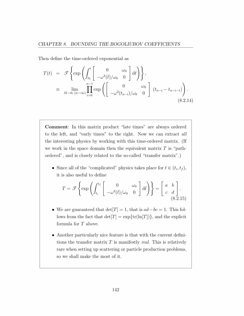
CHAPTER 8. BOUNDING THE BOGOLIUBOV COEFFICIENTS
Then define the time-ordered exponential as
T (t) = T
exp
(∫ t
t0
[0 ω0
−ω2(t)/ω0 0
]dt
),
≡ limM→0, (n→∞)
n−1∏i=0
exp
([0 ω0
−ω2(tn−i)/ω0 0
](tn−i − tn−i−1)
).
(8.2.14)
Comment: In this matrix product “late times” are always ordered
to the left, and “early times” to the right. Now we can extract all
the interesting physics by working with this time-ordered matrix. (If
we work in the space domain then the equivalent matrix T is “path-
ordered”, and is closely related to the so-called “transfer matrix”.)
• Since all of the “complicated” physics takes place for t ∈ (ti, tf ),
it is also useful to define
T = T
exp
(∫ tf
ti
[0 ω0
−ω2(t)/ω0 0
]dt
)=
[a b
c d
].
(8.2.15)
• We are guaranteed that det[T ] = 1, that is ad−bc = 1. This fol-
lows from the fact that det[T ] = exptr(ln[T ]), and the explicit
formula for T above.
• Another particularly nice feature is that with the current defini-
tions the transfer matrix T is manifestly real. This is relatively
rare when setting up scattering or particle production problems,
so we shall make the most of it.
142
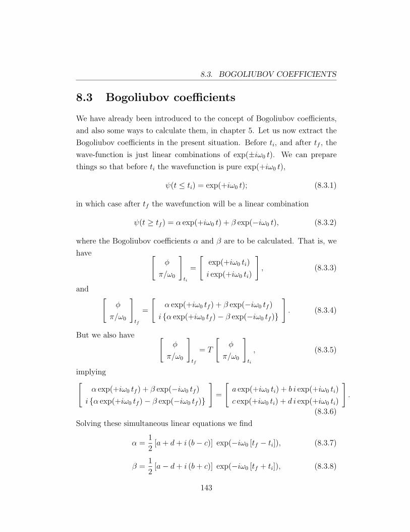
8.3. BOGOLIUBOV COEFFICIENTS
8.3 Bogoliubov coefficients
We have already been introduced to the concept of Bogoliubov coefficients,
and also some ways to calculate them, in chapter 5. Let us now extract the
Bogoliubov coefficients in the present situation. Before ti, and after tf , the
wave-function is just linear combinations of exp(±iω0 t). We can prepare
things so that before ti the wavefunction is pure exp(+iω0 t),
ψ(t ≤ ti) = exp(+iω0 t); (8.3.1)
in which case after tf the wavefunction will be a linear combination
ψ(t ≥ tf ) = α exp(+iω0 t) + β exp(−iω0 t), (8.3.2)
where the Bogoliubov coefficients α and β are to be calculated. That is, we
have [φ
π/ω0
]ti
=
[exp(+iω0 ti)
i exp(+iω0 ti)
], (8.3.3)
and [φ
π/ω0
]tf
=
[α exp(+iω0 tf ) + β exp(−iω0 tf )
i α exp(+iω0 tf )− β exp(−iω0 tf )
]. (8.3.4)
But we also have [φ
π/ω0
]tf
= T
[φ
π/ω0
]ti
, (8.3.5)
implying[α exp(+iω0 tf ) + β exp(−iω0 tf )
i α exp(+iω0 tf )− β exp(−iω0 tf )
]=
[a exp(+iω0 ti) + b i exp(+iω0 ti)
c exp(+iω0 ti) + d i exp(+iω0 ti)
].
(8.3.6)
Solving these simultaneous linear equations we find
α =1
2[a+ d+ i (b− c)] exp(−iω0 [tf − ti]), (8.3.7)
β =1
2[a− d+ i (b+ c)] exp(−iω0 [tf + ti]), (8.3.8)
143
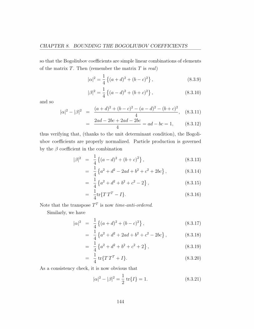
CHAPTER 8. BOUNDING THE BOGOLIUBOV COEFFICIENTS
so that the Bogoliubov coefficients are simple linear combinations of elements
of the matrix T . Then (remember the matrix T is real)
|α|2 =1
4
(a+ d)2 + (b− c)2
, (8.3.9)
|β|2 =1
4
(a− d)2 + (b+ c)2
, (8.3.10)
and so
|α|2 − |β|2 =(a+ d)2 + (b− c)2 − (a− d)2 − (b+ c)2
4, (8.3.11)
=2ad− 2bc+ 2ad− 2bc
4= ad− bc = 1, (8.3.12)
thus verifying that, (thanks to the unit determinant condition), the Bogoli-
ubov coefficients are properly normalized. Particle production is governed
by the β coefficient in the combination
|β|2 =1
4
(a− d)2 + (b+ c)2 , (8.3.13)
=1
4
a2 + d2 − 2ad+ b2 + c2 + 2bc
, (8.3.14)
=1
4
a2 + d2 + b2 + c2 − 2
, (8.3.15)
=1
4trT T T − I. (8.3.16)
Note that the transpose T T is now time-anti-ordered.
Similarly, we have
|α|2 =1
4
(a+ d)2 + (b− c)2
, (8.3.17)
=1
4
a2 + d2 + 2ad+ b2 + c2 − 2bc
, (8.3.18)
=1
4
a2 + d2 + b2 + c2 + 2
, (8.3.19)
=1
4trT T T + I. (8.3.20)
As a consistency check, it is now obvious that
|α|2 − |β|2 =1
2trI = 1. (8.3.21)
144

8.4. ELEMENTARY BOUND:
Comment: We can always formally solve the relevant ODE, either
equation (8.2.1) or its equivalent equation (8.2.2), in terms of the
time-ordered exponential, and we can always formally extract the Bo-
goliubov coefficients in terms of traces of the form trT T T. We shall
now use these formal results to derive rigorous bounds on the Bogoli-
ubov coefficients.
8.4 Elementary bound:
Now consider the quantity
X(t) = T (t) T (t)T , (8.4.1)
= T
exp
(∫ t
ti
[0 ω0
−ω2(t)/ω0 0
]dt
)
×
[T
exp
(∫ t
ti
[0 ω0
−ω2(t)/ω0 0
]dt
)]T. (8.4.2)
This object satisfies the differential equation
dX
dt=
[0 ω0
−ω2(t)/ω0 0
]X(t) +X(t)
[0 −ω2(t)/ω0
ω0 0
], (8.4.3)
with the boundary condition
X(ti) = I. (8.4.4)
Now note
tr(X) = trT T T = a2 + b2 + c2 + d2. (8.4.5)
145

CHAPTER 8. BOUNDING THE BOGOLIUBOV COEFFICIENTS
Furthermore
dX
dt=
[0 ω0
−ω2/ω0 0
][a2 + b2 ac+ bd
ac+ bd c2 + d2
]
+
[a2 + b2 ac+ bd
ac+ bd c2 + d2
][0 −ω2/ω0
ω0 0
],
=
[2ω0(ac+ bd) ω0(c2 + d2)− (ω2/ω0)(a2 + b2)
ω0(c2 + d2)− (ω2/ω0)(a2 + b2) (−2ω2/ω0)(ac+ bd)
],
(8.4.6)
and so we see
tr
[0 ω0
−ω2/ω0 0
]X +X
[0 −ω2/ω0
ω0 0
]= 2(ac+ bd)
[ω0 −
ω2
ω0
].
(8.4.7)
Thereforedtr[X]
dt= 2(ac+ bd)
[ω0 −
ω2
ω0
]. (8.4.8)
Using this key result, and some very simple analysis, we shall now derive our
first elementary bound on the Bogoliubov coefficients.
• For any 2 real numbers, using (x+ y)2 ≥ 0 and (x− y)2 ≥ 0, we have
x2 + y2 ≥ 2|xy|. (8.4.9)
In particular, for any 4 real numbers this implies
a2 + b2 + c2 + d2 ≥ 2√
(a2 + b2)(c2 + d2). (8.4.10)
• But we also have
|ac+ bd|2 + |ad− bc|2 = a2c2 + 2abcd+ b2d2 + a2d2 − 2abcd+ b2c2,
(8.4.11)
= (a2 + b2)(c2 + d2), (8.4.12)
thus, for any 4 real numbers
a2 + b2 + c2 + d2 ≥ 2√|ac+ bd|2 + |ad− bc|2. (8.4.13)
146
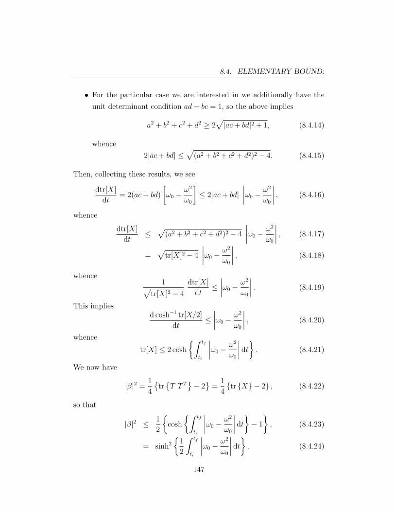
8.4. ELEMENTARY BOUND:
• For the particular case we are interested in we additionally have the
unit determinant condition ad− bc = 1, so the above implies
a2 + b2 + c2 + d2 ≥ 2√|ac+ bd|2 + 1, (8.4.14)
whence
2|ac+ bd| ≤√
(a2 + b2 + c2 + d2)2 − 4. (8.4.15)
Then, collecting these results, we see
dtr[X]
dt= 2(ac+ bd)
[ω0 −
ω2
ω0
]≤ 2|ac+ bd|
∣∣∣∣ω0 −ω2
ω0
∣∣∣∣ , (8.4.16)
whence
dtr[X]
dt≤
√(a2 + b2 + c2 + d2)2 − 4
∣∣∣∣ω0 −ω2
ω0
∣∣∣∣ , (8.4.17)
=√
tr[X]2 − 4
∣∣∣∣ω0 −ω2
ω0
∣∣∣∣ , (8.4.18)
whence1√
tr[X]2 − 4
dtr[X]
dt≤∣∣∣∣ω0 −
ω2
ω0
∣∣∣∣ . (8.4.19)
This impliesd cosh−1 tr[X/2]
dt≤∣∣∣∣ω0 −
ω2
ω0
∣∣∣∣ , (8.4.20)
whence
tr[X] ≤ 2 cosh
∫ tf
ti
∣∣∣∣ω0 −ω2
ω0
∣∣∣∣ dt . (8.4.21)
We now have
|β|2 =1
4
trT T T
− 2
=1
4tr X − 2 , (8.4.22)
so that
|β|2 ≤ 1
2
cosh
∫ tf
ti
∣∣∣∣ω0 −ω2
ω0
∣∣∣∣ dt− 1
, (8.4.23)
= sinh2
1
2
∫ tf
ti
∣∣∣∣ω0 −ω2
ω0
∣∣∣∣ dt . (8.4.24)
147

CHAPTER 8. BOUNDING THE BOGOLIUBOV COEFFICIENTS
So finally
|β|2 ≤ sinh2
1
2
∫ tf
ti
∣∣∣∣ω0 −ω2
ω0
∣∣∣∣ dt , (8.4.25)
and consequently
|α|2 ≤ cosh2
1
2
∫ tf
ti
∣∣∣∣ω0 −ω2
ω0
∣∣∣∣ dt . (8.4.26)
These bounds are quite remarkable in their generality. A version of this
result was derived in [88] but the present derivation is largely independent
and has the virtue of being completely elementary — in particular, the use
of complex numbers has been minimized, and we have absolutely eliminated
the use of the “auxiliary functions” and “gauge conditions” that were needed
for the derivation in [88]. If one translates this to the space domain, then
the equivalent barrier penetration coefficient is Ttransmission ↔ 1/|α|2, and the
equivalent reflection coefficient is R ↔ |β|2/|α|2. Making the appropriate
translations
Ttransmission ≥ sech2
1
2
∫ xf
xi
∣∣∣∣k0 −k2(x)
k0
∣∣∣∣ dx , (8.4.27)
and
R ≤ tanh2
1
2
∫ xf
xi
∣∣∣∣k0 −k2(x)
k0
∣∣∣∣ dx . (8.4.28)
Comment: For completeness we mention that reference [88] provides
a large number of consistency checks on these bounds by comparing
them with known exact results [117].
148

8.5. LOWER BOUND ON |β|2
8.5 Lower bound on |β|2
To obtain a lower bound on the |β| Bogoliubov coefficient, consider any real
valued parameter ε. Then since the matrix T is itself real,
tr
(T − ε T T )T (T − ε T T )≥ 0, (8.5.1)
so that
(1 + ε2) tr(T T T )− 2ε tr(T 2) ≥ 0, (8.5.2)
whence
tr(T T T ) ≥ 2ε
1 + ε2tr(T 2), (8.5.3)
This bound is extremized for ε = ±1, whence
tr(T T T ) ≥∣∣tr(T 2)
∣∣ , (8.5.4)
and so
|β|2 ≥ 1
4
∣∣tr(T 2)∣∣− 2
. (8.5.5)
This is certainly a bound, but it is not as useful as one might hope. It is
useful only if tr[T 2] > 2. But
tr[T 2] = a2+d2+2bc = a2+d2+2(ad−1) = (a+d)2−2 = (tr[T ])2−2. (8.5.6)
So using the unit determinant condition, tr[T 2] > 2 can be seen to require
|a + d| ≥ 2, that is, tr[T ] > 2. But when does this happen? For the real
matrix [a b
c d
](8.5.7)
with unit determinant the eigenvalues are
λ =a+ d
2±√
(a+ d)2 − 4
2. (8.5.8)
The condition a+d > 2 is thus equivalent to the condition that the eigenval-
ues are real. Unfortunately there seems to be no simple way to then relate
this to the properties of the function ω(t).
149

CHAPTER 8. BOUNDING THE BOGOLIUBOV COEFFICIENTS
8.6 A more general upper bound
Now let Ω(t) be an arbitrary everywhere real and nonzero function of t
with the dimensions of frequency. Then we can rewrite the Schrodinger
ODE (8.2.1) as:
d
dt
[φ√
Ω
π/√
Ω
]=
[12(Ω/Ω) Ω
−ω2(t)/Ω −12(Ω/Ω)
] [φ√
Ω
π/√
Ω
]. (8.6.1)
Again all the matrix elements have been carefully chosen to have the same
engineering dimension. Again we can formally solve this in terms of the
time-ordered product:[φ√
Ω
π/√
Ω
]t
= T
exp
(∫ t
t0
[12(Ω/Ω) Ω
−ω2(t)/Ω −12(Ω/Ω)
]dt
) [φ
π/√
Ω
]t0
.
(8.6.2)
The new T matrix is
T = T
exp
(∫ tf
ti
[12(Ω/Ω) Ω
−ω2(t)/Ω −12(Ω/Ω)
]dt
). (8.6.3)
Note that the matrix T is still real, and that because
tr
[12(Ω/Ω) Ω
−ω2(t)/Ω −12(Ω/Ω)
]= 0. (8.6.4)
it still follows that T has determinant unity:
T =
[a b
c d
]; ad− bc = 1. (8.6.5)
This means that much of the earlier computations carry through without
change. In particular as long as at the initial and final times we impose
Ω(t)→ ω0 as t→ tf and t→ ti, we still have
α =1
2[a+ d+ i (b− c)] exp(−iω0[tf − ti]), (8.6.6)
150

8.6. A MORE GENERAL UPPER BOUND
β =1
2[a− d+ i (b+ c)] exp(−iω0[tf + ti]), (8.6.7)
|β|2 =1
4trT T T − I
, (8.6.8)
|α|2 =1
4trT T T + I
. (8.6.9)
Now consider the quantity
X(t) = T (t) T (t)T = T
exp
(∫ t
ti
[12(Ω/Ω) Ω
−ω2(t)/Ω −12(Ω/Ω)
]dt
)
×
[T
exp
(∫ t
ti
[12(Ω/Ω) Ω
−ω2(t)/Ω −12(Ω/Ω)
]dt
)]T.
(8.6.10)
This now satisfies the differential equation
dX
dt=
[12(Ω/Ω) Ω
−ω2(t)/Ω −12(Ω/Ω)
]X +X
[12(Ω/Ω) −ω2(t)/Ω
Ω −12(Ω/Ω)
], (8.6.11)
with the boundary condition
X(ti) = I, (8.6.12)
and
tr[X] = a2 + b2 + c2 + d2. (8.6.13)
A brief computation yields
dX
dt=
[12(Ω/Ω) Ω
−ω2(t)/Ω −12(Ω/Ω)
][a2 + b2 ac+ bd
ac+ bd c2 + d2
]
+
[a2 + b2 ac+ bd
ac+ bd c2 + d2
][12(Ω/Ω) −ω2(t)/Ω
Ω −12(Ω/Ω)
],
(8.6.14)
=
[(Ω/Ω)(a2 + b2) + 2Ω(ac+ bd) Ω(c2 + d2)− (ω2/Ω)(a2 + b2)
−(ω2/Ω)(a2 + b2) + Ω(c2 + d2) −(2ω2/Ω)(ac+ bd)− (Ω/Ω)(c2 + d2)
].
(8.6.15)
151

CHAPTER 8. BOUNDING THE BOGOLIUBOV COEFFICIENTS
Then taking the trace, there is now one extra term
dtr[X]
dt= (a2 + b2 − c2 − d2)
[Ω
Ω
]+ 2(ac+ bd)
[Ω− ω2
Ω
]. (8.6.16)
Note that if Ω(t) → ω0 then Ω → 0 and we recover the ODE of the “ele-
mentary” bound. In this more general setting we now proceed by using the
following facts:
• As previously we note
|ac+ bd|2 + |ad− bc|2 = a2c2 + 2abcd+ b2d2 + a2d2 − 2abcd+ b2c2,
= (a2 + b2)(c2 + d2),
(8.6.17)
which implies
|ac+ bd| =√
(a2 + b2)(c2 + d2)− 1, (8.6.18)
that is
2|ac+ bd| =√
4(a2 + b2)(c2 + d2)− 4. (8.6.19)
• Additionally, we use
|a2 + b2 − c2 − d2| =√|a2 + b2 + c2 + d2|2 − 4(a2 + b2)(c2 + d2),
(8.6.20)
implying
|a2 + b2 − c2 − d2|2 + (2|ac+ bd|)2 = |a2 + b2 + c2 + d2|2 − 4. (8.6.21)
In particular, combining these observations, this means that we can find an
angle θ (which is in general some complicated real function of a, b, c, d) such
that
2(ac+ bd) =√|a2 + b2 + c2 + d2|2 − 4 sin θ, (8.6.22)
a2 + b2 − c2 − d2 =√|a2 + b2 + c2 + d2|2 − 4 cos θ, (8.6.23)
152

8.6. A MORE GENERAL UPPER BOUND
whence
dtr[X]
dt=√|a2 + b2 + c2 + d2|2 − 4
sin θ
[Ω
Ω
]+ cos θ
[Ω− ω2
Ω
].
(8.6.24)
But for any real θ we certainly have by the Cauchy–Schwartz inequality
sin θ
[Ω
Ω
]+ cos θ
[Ω− ω2
Ω
]≤
√√√√[Ω
Ω
]2
+
[Ω− ω2
Ω
]2
, (8.6.25)
implying
dtr[X]
dt≤√|a2 + b2 + c2 + d2|2 − 4
√√√√[Ω
Ω
]2
+
[Ω− ω2
Ω
]2
. (8.6.26)
Therefore
dtr[X]
dt≤√
tr[X]2 − 4
√√√√[Ω
Ω
]2
+
[Ω− ω2
Ω
]2
, (8.6.27)
implying
1√tr[X]2 − 4
dtr[X]
dt≤
√√√√[Ω
Ω
]2
+
[Ω− ω2
Ω
]2
, (8.6.28)
whence
d cosh−1(tr[X]/2)
dt≤
√√√√[Ω
Ω
]2
+
[Ω− ω2
Ω
]2
, (8.6.29)
so that
tr[X] = tr[T T T ] ≤ 2 cosh
∫ tf
ti
√√√√[Ω
Ω
]2
+
[Ω− ω2
Ω
]2
dt
. (8.6.30)
Using the general formulae for |α|2 and |β|2 in terms of trT T T, and sim-
plifying, we see
|β|2 ≤ sinh2
1
2
∫ tf
ti
1
|Ω|
√Ω2 + [Ω2 − ω2]2 dt
, (8.6.31)
153

CHAPTER 8. BOUNDING THE BOGOLIUBOV COEFFICIENTS
and
|α|2 ≤ cosh2
1
2
∫ tf
ti
1
|Ω|
√Ω2 + [Ω2 − ω2]2 dt
. (8.6.32)
This result is completely equivalent to the corresponding result in [88]; though
again note that the derivation is largely independent and that it no longer
requires one to introduce any “gauge fixing” condition, nor need we intro-
duce any WKB-like ansatz. The current proof is much more “direct”, and at
worst uses simple inequalities and straightforward ODE theory. If we work
in the space domain instead of the time domain and make the translations
Ω(t)→ ϕ′(x), ω(t)→ k(x), we see
|α|2 ≤ cosh2
1
2
∫ xf
xi
1
|ϕ′|
√(ϕ′′)2 + [(ϕ′)2 − k2]2 dx
, (8.6.33)
and
|β|2 ≤ sinh2
1
2
∫ xf
xi
1
|ϕ′|
√(ϕ′′)2 + [(ϕ′)2 − k2]2 dx
. (8.6.34)
This is perhaps physically more transparent in terms of the equivalent trans-
mission and reflection coefficients
Ttransmission ≥ sech2
1
2
∫ xf
xi
1
|ϕ′|
√(ϕ′′)2 + [(ϕ′)2 − k2]2 dx
, (8.6.35)
and
R ≤ tanh2
1
2
∫ xf
xi
1
|ϕ′|
√(ϕ′′)2 + [(ϕ′)2 − k2]2 dx
. (8.6.36)
Comment: For completeness we mention that reference [88] provides
a number of consistency checks on these more general bounds by com-
paring them with known exact results [117].
154

8.7. THE “OPTIMAL” CHOICE OF Ω(T )?
8.7 The “optimal” choice of Ω(t)?
What is the optimal choice of Ω(t) that one can make leading to the most
stringent bound on the Bogoliubov coefficients? The bound we have just
derived holds for arbitrary Ω(t), subject to the two boundary conditions
Ω(ti) = ω0 = Ω(tf ) and the overall constraint Ω(t) 6= 0. Since both sinh and
cosh are convex functions, finding the most stringent constraint on |β| and
|α| is thus a variational calculus problem equivalent to minimizing the action
S =
∫ tf
ti
1
|Ω|
√Ω2 + [Ω2 − ω2]2 dt. (8.7.1)
The relevant Euler–Lagrange equations are quite messy, and progress (at
least insofar as there is any practicable progress) is better made by using an
indirect attack. The Lagrangian is
L =1
|Ω|
√Ω2 + [Ω2 − ω2]2, (8.7.2)
and so the corresponding canonical momentum can be evaluated as
π =∂L
∂Ω=
Ω
|Ω|√
Ω2 + [Ω2 − ω2]2. (8.7.3)
From the boundary conditions we can deduce
π(ti) =1
ω0
= π(tf ). (8.7.4)
The Hamiltonian is now
H = π Ω− L =Ω2 −
Ω2 + [Ω2 − ω2]
2
|Ω|√
Ω2 + [Ω2 − ω2]2= − [Ω2 − ω2]
2
|Ω|√
Ω2 + [Ω2 − ω2]2.
(8.7.5)
Unfortunately the Hamiltonian is explicitly time-dependent [via ω(t)] and
so is not conserved. The best we can say is that at the endpoints of the motion
H(ti) = 0 = H(tf ). (8.7.12)
155

CHAPTER 8. BOUNDING THE BOGOLIUBOV COEFFICIENTS
Hamiltonian (classical mechanics): For a closed system the sum
of the kinetic and potential energy in the system is represented by a
quantity called the Hamiltonian, which leads to a set of differential
equations known as the Hamilton equations for that system [107].
The Hamilton equations are generally written as follows:
p = −∂H∂q
, (8.7.6)
q =∂H∂p
, (8.7.7)
the dot denotes the ordinary derivative with respect to time of the
functions p = p(t) (called generalized momenta) and q = q(t) (called
generalized coordinates), and H = H(p, q, t) is the so-called Hamilto-
nian. Thus, a little more explicitly, one can equivalently write
d
dtp(t) = − ∂
∂qH(p(t), q(t), t), (8.7.8)
d
dtq(t) =
∂
∂pH(p(t), q(t), t), (8.7.9)
and specify the domain of values in which the parameter t (“time”)
varies.
By solving for Ω as a function of π and Ω we can also write
Ω =πΩ√
1− π2 Ω2(Ω2 − ω2), (8.7.13)
and
H = −√
1− π2 Ω2 (Ω2 − ω2)
|Ω|. (8.7.14)
Note that Ω at the endpoints cannot in general be explicitly evaluated in
terms of the boundary conditions.
An alternative formulation which slightly simplifies the analysis is to
156

8.7. THE “OPTIMAL” CHOICE OF Ω(T )?
Hamiltonian (quantum mechanics): The Hamiltonian H is the
quantum mechanical operator corresponding to the total energy of the
system. It generates the time evolution of quantum states. If |ψ(t)〉is the state of the system at time t, then [106]
H|ψ(t)〉 = i~∂
∂t|ψ(t)〉, (8.7.10)
where ~ is the reduced Planck constant. This equation is known as
the (time dependent) Schrodinger equation. (This is the same form
as the Hamilton-Jacobi equation, which is one of the reasons H is also
called the Hamiltonian.) Given the state at some initial time (t = 0),
we can integrate it to derive the state at any subsequent time. If H is
independent of time, then
|ψ(t)〉 = exp
(− iHt
~
)|ψ(0)〉. (8.7.11)
In this thesis we are sometimes using quantum Hamiltonians, and
sometimes classical Hamiltonians. Whether we are in a quantum or
classical situation will have to be determined from context.
change variables by writing
Ω(t) = ω0 exp[θ(t)], (8.7.15)
where the boundary conditions are now
θ(ti) = 0 = θ(tf ), (8.7.16)
and the action is now rewritten as
S =
∫ tf
ti
√θ2 + ω2
0
[e2θ − ω2
ω20
e−2θ
]2
dt. (8.7.17)
157
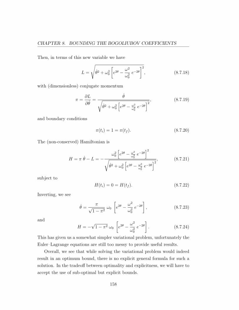
CHAPTER 8. BOUNDING THE BOGOLIUBOV COEFFICIENTS
Then, in terms of this new variable we have
L =
√θ2 + ω2
0
[e2θ − ω2
ω20
e−2θ
]2
, (8.7.18)
with (dimensionless) conjugate momentum
π =∂L
∂θ=
θ√θ2 + ω2
0
[e2θ − ω2
ω20e−2θ
]2, (8.7.19)
and boundary conditions
π(ti) = 1 = π(tf ). (8.7.20)
The (non-conserved) Hamiltonian is
H = π θ − L = −ω2
0
[e2θ − ω2
ω20e−2θ
]2
√θ2 + ω2
0
[e2θ − ω2
ω20e−2θ
]2, (8.7.21)
subject to
H(ti) = 0 = H(tf ). (8.7.22)
Inverting, we see
θ =π√
1− π2ω0
[e2θ − ω2
ω20
e−2θ
], (8.7.23)
and
H = −√
1− π2 ω0
[e2θ − ω2
ω20
e−2θ
]. (8.7.24)
This has given us a somewhat simpler variational problem, unfortunately the
Euler–Lagrange equations are still too messy to provide useful results.
Overall, we see that while solving the variational problem would indeed
result in an optimum bound, there is no explicit general formula for such a
solution. In the tradeoff between optimality and explicitness, we will have to
accept the use of sub-optimal but explicit bounds.
158

8.8. SUB-OPTIMAL BUT EXPLICIT BOUNDS
8.8 Sub-optimal but explicit bounds
From our general bounds
|β|2 ≤ sinh2
1
2
∫ tf
ti
1
|Ω|
√Ω2 + [Ω2 − ω2]2 dt
, (8.8.1)
and
|α|2 ≤ cosh2
1
2
∫ tf
ti
1
|Ω|
√Ω2 + [Ω2 − ω2]2 dt
, (8.8.2)
the following special cases are of particular interest:
Ω = ω0: In this case we simply obtain the “elementary” bound considered
above.
Ω = ω: This case only makes sense if ω2 > 0 is always positive. (Otherwise
ω and hence Ω becomes imaginary in the “classically forbidden” region;
the matrix T then becomes complex, and the entire formalism breaks
down). Subject to this constraint we find
|β|2 ≤ sinh2
1
2
∫ tf
ti
∣∣∣∣ ωω∣∣∣∣ dt
, (8.8.3)
and
|α|2 ≤ cosh2
1
2
∫ tf
ti
∣∣∣∣ ωω∣∣∣∣ dt
. (8.8.4)
This case was also considered in [88].
Ω = ωε ω1−ε0 : This case again only makes sense if ω2 > 0 is always positive.
Subject to this constraint we find
|β|2 ≤ sinh2
1
2
∫ tf
ti
√ε2ω2
ω2+ω2ε[ω2−2ε
0 − ω2−2ε]2
ω2−2ε0
dt
, (8.8.5)
and
|α|2 ≤ cosh2
1
2
∫ tf
ti
√ε2ω2
ω2+ω2ε[ω2−2ε
0 − ω2−2ε]2
ω2−2ε0
dt
. (8.8.6)
This nicely interpolates between the two cases given above, which cor-
respond to ε = 0 and ε = 1 respectively.
159

CHAPTER 8. BOUNDING THE BOGOLIUBOV COEFFICIENTS
Comment: The WKB approximation technique provides an approx-
imate solution to the Schrodinger equation (8.2.3) of a quantum me-
chanical system; however this technique fails at the classical turning
points of the system of the potential energy function, V (x) [111].
Standard WKB theory provides a set of “joining conditions” for “step-
ping over” the turning points and penetrating into the classically for-
bidden region. Unfortunately we do not seem to have any analogue of
these “joining conditions” in the formalism we set up in this thesis.
Triangle inequality: Since√x2 + y2 ≤ |x|+ |y| we see that
|β|2 ≤ sinh2
1
2
∫ tf
ti
∣∣∣∣∣ΩΩ∣∣∣∣∣ dt+
1
2
∫ tf
ti
∣∣∣∣Ω− ω2
Ω
∣∣∣∣ dt
, (8.8.7)
and
|α|2 ≤ cosh2
1
2
∫ tf
ti
∣∣∣∣∣ΩΩ∣∣∣∣∣ dt+
1
2
∫ tf
ti
∣∣∣∣Ω− ω2
Ω
∣∣∣∣ dt
. (8.8.8)
These bounds, because they are explicit, are often the most useful quantities
to calculate.
160

8.9. THE “INTERACTION PICTURE”
8.9 The “interaction picture”
Interaction picture (sometimes called the Dirac picture): This
is an intermediate between the Schrodinger picture and the Heisenberg
picture. Whereas in the other two pictures either the state vector or
the operators carry time dependence, in the interaction picture both
carry part of the time dependence of observables. Equations that in-
clude operators acting at different times, which hold in the interaction
picture, do not necessarily hold in the Schrodinger or the Heisenberg
picture. This is because time-dependent unitary transformations re-
late operators in one picture to the analogous operators in the oth-
ers [109].
For our purposes the interaction picture is useful because it lets us
develop a perturbation theory.
If we split the function ω(t)2 into an exactly solvable piece ωe(t)2 and a
perturbation ω∆(t)2 then we can develop a formal perturbation series for the
transfer matrix T , in close analogy to the procedures for developing quantum
field theoretic perturbation theory in the interaction picture. Specifically let
us write
ω(t)2 = ωe(t)2 + ω∆(t)2, (8.9.1)
anddT (t)
dt= Q(t) T (t) = [Qe(t) +Q∆(t)] T (t). (8.9.2)
Now defining
T (t) = Te(t) T∆(t), (8.9.3)
we shall develop a formal solution for T∆(t). Consider
dT (t)
dt= [Qe(t) +Q∆(t)] Te(t) T∆(t), (8.9.4)
161
CHAPTER 8. BOUNDING THE BOGOLIUBOV COEFFICIENTS
and compare it with
dT (t)
dt=
dTe(t)
dtT∆(t) + Te(t)
dT∆(t)
dt= Qe(t) Te(t) T∆(t) + Te(t)
dT∆(t)
dt.
(8.9.5)
ThereforedT∆(t)
dt=Te(t)
−1 Q∆(t) Te(t)T∆, (8.9.6)
whence
T∆(t) = T exp
(∫ t
ti
Te(t)
−1 Q∆(t) Te(t)
dt
). (8.9.7)
For the full transfer matrix T we have
T (t) = Te(t)×T exp
(∫ t
ti
Te(t)
−1 Q∆(t) Te(t)
dt
), (8.9.8)
and we have succeeded in splitting it into an exact piece Te(t) plus a distortion
due to Q∆(t). This can now be used as the starting point for a perturbation
expansion. (The analogy with quantum field theoretic perturbation theory
in the interaction picture should now be completely clear.)
To develop some formal bounds on the Bogoliubov coefficients it is useful
to suppress (currently) unnecessary phases by defining
α =1
2[a+ d+ i (b− c)] , (8.9.9)
β =1
2[a− d+ i (b+ c)] . (8.9.10)
The virtue of these definitions is that for T = Te T∆ they satisfy a simple
composition rule which can easily be verified via matrix multiplication. From
T = Te T∆ we have[a b
c d
]=
[ae a∆ + be c∆ ae b∆ + be d∆
ce a∆ + de c∆ ce b∆ + de d∆
]. (8.9.11)
Then some simple linear algebra leads to
β = αe β∆ + βe α∗∆, (8.9.12)
162

8.10. CONCLUSION
α = αe α∆ + βe β∗∆, (8.9.13)
But then
|β| = |β| =∣∣∣αe β∆ + βe α
∗∆
∣∣∣ ≤ ∣∣∣αe β∆
∣∣∣+∣∣∣βe α∗∆∣∣∣ = |αe β∆|+ |βe α∆| ,
(8.9.14)
that is
|β| ≤ |αe| |β∆|+ |βe| |α∆| , (8.9.15)
or the equivalent
|β| ≤√
1 + |βe|2 |β∆|+ |βe|√
1 + |β∆|2. (8.9.16)
Similarly
|β| = |β| =∣∣∣αe β∆ + βe α
∗∆
∣∣∣ ≥ ∣∣∣ ∣∣∣αe β∆
∣∣∣− ∣∣∣βe α∗∆∣∣∣ ∣∣∣ = | |αe β∆| − |βe α∆| | ,(8.9.17)
that is
|β| ≥ | |αe| |β∆| − |βe| |α∆| | , (8.9.18)
or the equivalent
|β| ≥∣∣∣∣ √1 + |βe|2 |β∆| − |βe|
√1 + |β∆|2
∣∣∣∣ . (8.9.19)
The benefit now is that one has bounded the Bogoliubov coefficient in terms
of the (assumed known) exact coefficient βe and the contribution from the
perturbation β∆. Suitably choosing the split between exact and perturbative
contributions to ω2, one could in principle obtain arbitrarily accurate bounds.
8.10 Conclusion
In this chapter we again considered rigorous bounds on transmission, re-
flection, and Bogoliubov coefficients. In particular, the most outstanding
features of this chapter are:
163

CHAPTER 8. BOUNDING THE BOGOLIUBOV COEFFICIENTS
• We have re-considered the general bounds on the Bogoliubov coeffi-
cients developed in [88]. Additionally, we have seen how to extend the
bounds in [88] in many different ways. Moreover, we do not need to
“gauge fix”, nor do we need to appeal to any “WKB-like ansatz” to get
the discussion started.
• We have formulated some rigorous bounds that we can place on barrier
penetration probabilities, or equivalently on the Bogoliubov coefficients
associated with a time-dependent potential. Furthermore, we have not
seen anything like these bounds anywhere else.
• In addition, probably there are “optimal” bounds still waiting to be
discovered.
• It is apparent that the current bounds are not the best that can be
achieved, and we strongly suspect that it may be possible to develop
yet further extensions to the current formalism.
Considering the fundamental importance of the questions we are asking,
it is remarkable how little work on this topic can currently be found in the
literature.
Possible extensions might include somehow relaxing the reality constraint
on Ω(t) without damaging too much of the current formalism, a better under-
standing of the variational problem defining the “optimal” bound (thus hope-
fully leading to an explicit form thereof), or using several “probe functions”
[instead of the single function Ω(t)] to more closely bound the Bogoliubov
coefficients.
164

Chapter 9
Bounding the greybody factors
for Schwarzschild black holes
9.1 Introduction
Black hole greybody factors are important because they modify the spectrum
of Hawking radiation seen at spatial infinity [74], so that it is not quite
Planckian [75]. (That is, it is no longer exactly “blackbody radiation”, which
is why [with slight abuse of language], it is called “greybody”.) There is a
vast scientific literature dealing with estimates of these black-hole greybody
factors, using a wide variety of techniques [90].
Unfortunately, most of these calculations adopt various approximations
that move one away from the physically most important regions of parameter
space. Sometimes one is forced into the extremal limit, sometimes one is
forced to asymptotically high or low frequencies, sometimes techniques work
only away from (3+1) dimensions, sometimes the nature of the approximation
is uncontrolled. As a specific example, monodromy techniques fail for s = 1
(photons) [77], which is observationally one of the most important cases one
would wish to consider.
Faced with these limitations, in this chapter we ask a slightly different
question: Restricting attention to the physically most important situations
165

CHAPTER 9. BOUNDING THE GREYBODY FACTORS
(Schwarzschild black holes, (3+1) dimensions, intermediate frequencies, un-
constrained spin and angular momentum) is it possible to at least place
rigorous (and hopefully simple) analytic bounds on the greybody factors?
By now considering the Regge–Wheeler equation for excitations around
Schwarzschild spacetime, and adapting the general analysis discussed in ear-
lier sections of this thesis, and published in references [88, 89], we shall
demonstrate that rigorous analytic bounds are indeed achievable. While it is
certainly true that these bounds may not answer all the physical questions
one might legitimately wish to ask, they are definitely a solid step in the
right direction.
Before starting the detailed calculations for this chapter, we should stress
some important issues related to the greybody factors in Schwarzschild black
holes:
• Hawking radiation was originally derived in the geometric optics ap-
proximation where it can be shown to be described by ideal black body
radiation — a black body is an object that absorbs all light that falls
on it. No electromagnetic radiation passes through it and none is re-
flected. Because no light is reflected or transmitted, the object appears
black when it is cold [121]. This derivation led to a calculation of the
temperature and entropy of a black hole.
• In this chapter, we shall try to rigorously solve for bounds on the trans-
mission probabilities for waves moving through the region of space out-
side of a Schwarzschild black hole — Schwarzschild black holes are the
simplest type, one that is described as a spherically symmetric body
with no (electric or magnetic) charge or angular momentum (no rota-
tion).
• The most important issue is to realise that “greybody factor” is actually
a synonym for “transmission probability”. Indeed, the phrase “grey-
body factor” is used more in the thermodynamics and spectroscopy
communities, while the phrase “transmission probability” is used more
166

9.2. HAWKING RADIATION
in the quantum mechanics community, but these communities are re-
ferring to the same concept.
• The greybody factor describes the emissivity of the black hole which is
not that of a perfect blackbody.
• As a black hole radiates energy by Hawking radiation, energy conser-
vation implies that it will lose mass.
Schwarzschild black hole or static black hole: This black hole
has no charge or angular momentum. A Schwarzschild black hole is
described by the Schwarzschild metric, and cannot be distinguished
from any other Schwarzschild black hole except by its mass. This
black hole is characterized by a spherical surface, called the event
horizon, which encloses the central singularity. The event horizon is
situated at the Schwarzschild radius, often called the radius of a black
hole.
Any spherically symmetric mass distribution whose radius is smaller
than the Schwarzschild radius forms a black hole [120].
9.2 Hawking radiation
A black body is an object that absorbs all light that falls on it. No electro-
magnetic radiation passes through it and none is reflected. Because no light
is reflected or transmitted, the object appears black when it is cold [121].
The light emitted by a black body is called black body radiation.
Hawking radiation is an approximately thermal radiation with an approx-
imately black body spectrum predicted to be emitted by black holes due to
quantum effects. It was discovered by Stephen Hawking who provided the
167

CHAPTER 9. BOUNDING THE GREYBODY FACTORS
Evaporating black holes: There are several significant consequences
that appear as a result of considering evaporating black holes:
(1) We first note that black hole evaporation generates a more consis-
tent view of black hole thermodynamics, by showing how black holes
interact thermally with the remainder of the universe.
(2) Secondly, the temperature of a black hole increases as it radiates
away mass. In fact, the rate of temperature rises as explosively, with
the most plausible of the endpoint scenarios being the complete disso-
lution of the black hole in a violent explosion of gamma rays. To make
a complete description of this assumed dissolution process, one would
need a model of quantum gravity, which would be needed in the fi-
nal stages of the evaporation process, when the black hole approaches
Planck mass and Planck radius. (The precise details of what is go-
ing on here is the subject of much continued, and sometimes heated,
debate.)
(3) Finally, the simplest models of black hole evaporation lead to the
black hole information paradox. For instance, the “information con-
tent” of a black hole appears to be lost when it evaporates, as under
many of these models the Hawking radiation is purely random. It
is felt by many (not all physicists) that the Hawking radiation must
be somehow perturbed to contain the missing information, that the
Hawking evaporation somehow carries the missing information to in-
finity. This would imply that information is not allowed to be lost
under these conditions [122]. (Technically, in this model the Hawking
evaporation process is asserted to be “unitary”. The precise details of
what is going on here is the subject of much continued, and sometimes
heated, debate [93, 94].)
168

9.3. REGGE–WHEELER EQUATION
Entropy: Black holes are truly thermodynamic systems with an ac-
tual and precisely calculable temperature and entropy. However, in
terms of statistical mechanics, the entropy should be the logarithm of
the number of independent states of the black hole. Understanding
how to count these states would constitute a significant progress in
the probe to understand quantum gravity [124]. (In this regard, some
string-based models have led to at least partial success.)
theoretical argument for its existence in 1974, and is closely related to work
by the physicist Jacob Bekenstein who predicted that black holes should have
a finite, non-zero entropy [122].
Greybody factors in black hole physics modify the naive Planckian spec-
trum that is predicted for Hawking radiation when working in the limit of
geometrical optics. We shall consider the Schwarzschild geometry in (3+1)
dimensions, and analyze the Regge–Wheeler equation for arbitrary particle
spin s and wave-mode angular momentum `, deriving rigorous bounds on the
greybody factors as a function of s, `, wave frequency ω, and the black hole
mass m.
9.3 Regge–Wheeler equation
The well-known Regge–Wheeler equation describes the axial perturbation
of Schwarzschild metric in the linear approximation [95]. In terms of the
tortoise coordinate r∗ the Regge–Wheeler equation (GN → 1) is
d2ψ
dr2∗
= [ω2 − V (r)]ψ, (9.3.1)
where for the specific case of a Schwarzschild black hole
dr
dr∗= 1− 2m
r, (9.3.2)
169

CHAPTER 9. BOUNDING THE GREYBODY FACTORS
Comment: The most standard interpretation of the Hawking radia-
tion theory states that implicit “virtual” particle-antiparticle pairs are
occasionally created outside the event horizon of a black hole. There
are three things that can happen to a pair of particles just outside the
event horizon [125]:
• Both particles are pulled into the black hole.
• Both particles escape from the black hole.
• One particle escapes while the other is pulled into the black hole.
In particular, the particle that has escaped becomes real and
can consequently be observed from Earth (or by any outside ob-
server). The particle that was pulled into the black hole remains
virtual, and to satisfy conservation of energy must have negative
mass-energy. The black hole absorbs this negative mass-energy
and as a result, loses mass and appears to shrink. The total
rate of power emission is (to an excellent approximation) pro-
portional to the inverse square of the black hole’s mass.
This is only a visual picture, at best an aid to understanding, and many
relativists would argue that the true situation can only be begun to
be understood by calculating the renormalized stress-energy tensor in
the vicinity of the horizon. Such calculations agree that the key point
is that negative energy is flowing into the black hole.
170

9.3. REGGE–WHEELER EQUATION
Quantum field theory in curved spacetime: Ordinary quantum
field theories are defined in flat Minkowski space, which is an outstand-
ingly good approximation for expressing the physics of microscopic
particles in weak gravitational fields like those seen on Earth.
In contrast, one can formulate quantum field theories in curved space-
time to describe situations in which gravity is powerful enough to
influence quantum matter, while, however, it is not powerful enough
to require quantization itself. Importantly, these theories depend on
classical general relativity to express a curved background spacetime.
A generalized quantum field theory is used to describe the behavior
of quantum matter within that spacetime. In addition, one can use
this formalism to show that black holes emit a blackbody spectrum of
particles known as Hawking radiation, leading to the possibility that
they evaporate over time. It is believed that this radiation represents
a significant part of the thermodynamics of black holes [4].
For our purposes, we will not be dealing with curved-space quantum
field theory directly. However, the general techniques we develop in
this thesis can be adapted to answer specific questions in curved-space
quantum field theory, such as placing limits on the transmission co-
efficients in black hole scattering, and bounding cosmological particle
production due to the expansion of the universe.
and the Regge–Wheeler potential is
V (r) =
(1− 2m
r
)[`(`+ 1)
r2+
2m(1− s2)
r3
]. (9.3.3)
Here s is the spin of the particle and ` is the angular momentum of the
specific wave mode under consideration, with ` ≥ s. Thus V (r) ≥ 0 outside
the horizon, where r ∈ (2m,∞). The greybody factors we are interested in
are just the transmission probabilities for wave modes propagating through
171

CHAPTER 9. BOUNDING THE GREYBODY FACTORS
this Regge–Wheeler potential.
Tortoise coordinate: In a Schwarzschild spacetime the so-called
“tortoise coordinate” is defined by [126]:
r∗ = r + 2GM ln
∣∣∣∣ r
2GM− 1
∣∣∣∣. (9.3.4)
The tortoise coordinate r∗ approaches −∞ as “r” approaches the
Schwarzschild radius r = 2GM . It satisfies
dr∗
dr=
(1− 2GM
r
)−1
. (9.3.5)
If we watch an object fall towards the Schwarzschild radius, then in
terms of the r coordinate the object seems to slow down and (asymp-
totically) stop at the horizon. In contrast,
dr∗
dt(9.3.6)
remains finite. In some vague analogy with the fable of the “tortoise
and the hare”, the r∗ coordinate has come to be known as the “tor-
toise” coordinate.
• Despite comments often encountered in the literature, one can explic-
itly solve for r as a function of the tortoise coordinate r∗ — in terms
of the Lambert W function we have the exact result
r(r∗) = 2m[1 +W (e[r∗−2m]/2m)
], (9.3.7)
whereas
r∗(r) = r + 2m ln
[r − 2m
2m
]. (9.3.8)
Unfortunately this formal result, while certainly correct and exact, is
less useful than one might suppose. (We have not been able to turn
this observation into any useful calculation.)
172

9.3. REGGE–WHEELER EQUATION
• Despite other comments often encountered in the literature, one can
also explicitly solve the Regge–Wheeler equation — now in terms of
Heun functions [95]. Unfortunately this is again less useful than one
might suppose, this time because relatively little is known about the
analytical behaviour of Heun functions — this is an area of ongoing
research in mathematical analysis [96].
Heun functions: In mathematics, the Heun differential equation is
a second-order linear ordinary differential equation of the form [127]
d2w
dz2+
[γ
z+
δ
z − 1+
ε
z − d
]dw
dz+
αβz − qz(z − 1)(z − d)
w = 0. (9.3.9)
Note that the constraint ε = α + β − γ − δ + 1 is needed to ensure
regularity of the singular point at ∞. Every second-order linear ODE
in the complex plane (or on the Riemann sphere, to be more accurate)
with four regular singular points can be transformed into this equation.
This standardized equation has four regular singular points: 0, 1, d,
and ∞.
Studying the properties of these functions is an area of ongoing re-
search in mathematical analysis [96].
173
CHAPTER 9. BOUNDING THE GREYBODY FACTORS
9.4 Bounds
The general bounds developed earlier in this thesis, and published in refer-
ences [88, 89], can, in the current situation, be written as
T ≥ sech2
∫ ∞−∞
ϑ dr∗
. (9.4.1)
Here T is the transmission probability (greybody factor), and ϑ is the func-
tion
ϑ =
√(h′)2 + [ω2 − V − h2]2
2h, (9.4.2)
where, h is some positive function, h(r∗) > 0, satisfying the limits h(−∞) =
h(+∞) = ω, which is otherwise arbitrary. Two different derivations of this
general result, and numerous consistency checks, can be found in earlier
chapters 5 and 8 of this thesis, and in references [88, 89].
(These bounds were originally developed as a technical step when study-
ing the completely unrelated issue of sonoluminescence [112], and since then
have also been used to place limits on particle production in analogue space-
times [83] and resonant cavities [84], to investigate qubit master equations [85],
and to motivate further general investigations of one-dimensional scattering
theory [86].) For current purposes, the most useful practical results are ob-
tained by considering two special cases:
1. If we set h = ω then
T ≥ sech2
1
2ω
∫ ∞−∞
V (r∗) dr∗
, (9.4.3)
whence
T ≥ sech2
1
2ω
∫ ∞2m
[`(`+ 1)
r2+
2m(1− s2)
r3
]dr
. (9.4.4)
Therefore, since the remaining integral is trivial, we obtain our first
explicit bound:
T ≥ sech2
2`(`+ 1) + (1− s2)
8ωm
. (9.4.5)
174

9.4. BOUNDS
That is:
T ≥ sech2
(`+ 1)2 + (`2 − s2)
8ωm
. (9.4.6)
Note that this bound is meaningful for all frequencies. This is sufficient
to tell us that at high frequencies the Regge–Wheeler barrier is almost
fully transparent, while even at arbitrarily low frequencies some nonzero
fraction of the Hawking flux will tunnel through. A particularly nice
feature of this first bound is that it is so easy to write down for arbitrary
s and `.
2. If we now set h =√ω2 − V , which in this case implicitly means that
we are not permitting any classically forbidden region, then
T ≥ sech2
1
2
∫ ∞−∞
∣∣∣∣h′h∣∣∣∣ dr∗
. (9.4.7)
Since for arbitrary s and ` the Regge–Wheeler potential is easily seen
to have a unique peak at which it is a maximum, this becomes
T ≥ sech2
ln
(hpeak
h∞
), (9.4.8)
= sech2
ln
(√ω2 − Vpeak
ω
), (9.4.9)
which is easily seen to be monotonic decreasing as a function of Vpeak.
However calculating the location of the peak, and value of the Regge–
Wheeler potential at the peak is somewhat more tedious than evaluat-
ing the previous bound (9.4.5). Note that the present bound fails, and
gives no useful information, once ω2 < Vpeak, corresponding to a clas-
sically forbidden region. More explicitly, the bound can be rewritten
as:
T ≥ 4ω2(ω2 − Vpeak)
(2ω2 − Vpeak)2= 1−
V 2peak
(2ω2 − Vpeak)2. (9.4.10)
The most interesting point of the study of black hole greybody factors [90],
and (once one moves into the complex plane), the closely related problem of
175

CHAPTER 9. BOUNDING THE GREYBODY FACTORS
Monodromy theorem: The monodromy theorem is a significant re-
sult regarding analytic continuation of a complex-analytic function to
a larger set. The basic concept is that one can extend a complex ana-
lytic function along curves — the process can be started in the original
domain of the function and can be ended in the bigger set. In addi-
tion, this theorem gives sufficient conditions for analytic continuation
to give the same value at a given point regardless of the specific curve
used to get there, so that the resulting extended analytic function
would be well-defined and single-valued [128].
locating the quasinormal modes [77, 97, 98], is a subject that has attracted
a wide amount of interest. In particular, quasinormal modes are poles of
the transmission coefficient and reflect the black hole’s ringdown reaction
to a perturbation [77]. Unfortunately, as a specific example, monodromy
techniques fail for s = 1 (photons) [77], which is observationally one of the
most important cases one would wish to consider. It is for this reason that
we resort to our general bounds to extract as much information as possible.
Let us now consider various sub-cases:
• For s = 1 (ie, photons) the situation simplifies considerably. (Remem-
ber, this is the case for which monodromy techniques fail [77].) For
s = 1 we always have rpeak = 3m and
Vpeak =`(`+ 1)
27m2. (9.4.11)
Consequently, from (9.4.10)
Ts=1 ≥108ω2m2[27ω2m2 − `(`+ 1)]
[54ω2m2 − `(`+ 1)]2. (9.4.12)
In almost the entire region where this bound applies (ω2 > Vpeak) it is
in fact a better bound than (9.4.5) above.
176

9.4. BOUNDS
• For s = 0 (ie, scalars) and ` = 0 (the s-wave), we have rpeak = 8m/3
and
Vpeak =27
1024m2. (9.4.13)
Consequently
Ts=0,`=0 ≥4096ω2m2[1024ω2m2 − 27]
[2048ω2m2 − 27]2. (9.4.14)
In a large fraction of the region where this bound applies it is in fact a
better bound than (9.4.5) above.
• For s = 0 but ` ≥ 1 it is easy to see that throughout the black hole
exterior, ∀r ∈ (2m,∞), we have
Vs=0,`≥1(r) <
(1− 2m
r
)[`2 + `+ 1
r2
], (9.4.15)
which is the s = 1 potential with the replacement `(`+ 1)→ `2 + `+ 1.
This bound on the potential has its maximum at rpeak = 3m, implying
Vpeak,s=0,`≥1 <`2 + `+ 1
27m2. (9.4.16)
Therefore the monotonicity of the bound on the greybody factor implies
Ts=0,`≥1 >108ω2m2[27ω2m2 − (`2 + `+ 1)]
[54ω2m2 − (`2 + `+ 1)]2, (9.4.17)
(for ω, m, and ` held fixed, and subject to s ≤ `).
• For s > 1 it is easy to see that throughout the black hole exterior, ∀r ∈(2m,∞), keeping ` held fixed, we have Vs>1(r) < Vs=1(r). Therefore
Vpeak,s>1 < Vpeak,s=1. (9.4.18)
Therefore the monotonicity of the bound on the greybody factor implies
Ts>1 >108ω2m2[27ω2m2 − `(`+ 1)]
[54ω2m2 − `(`+ 1)]2, (9.4.19)
(for ω, m, and ` held fixed, and subject to s ≤ `).
177

CHAPTER 9. BOUNDING THE GREYBODY FACTORS
• More generally, it is useful to define
ε =1− s2
`(`+ 1). (9.4.20)
Excluding the case (s, `) = (0, 0), which was explicitly dealt with above,
the remainder of the physically interesting region is confined to the
range ε ∈ (−1,+1/2]. Then a brief computation yields
rpeak = 3m
1− ε
9+O(ε2)
, (9.4.21)
and
Vpeak =`(`+ 1)
27m2
1 +
2ε
3+O(ε2)
. (9.4.22)
In fact one can show that
Vpeak <`(`+ 1)
20m2, (9.4.23)
over the physically interesting range. (This bound on Vpeak is tightest
for (s, `) = (0, 1), corresponding to ε = +1/2, where it provides a better
than 1% estimate, and becomes progressively weaker as one moves to
ε = −1.) This then implies
T(s,`)6=(0,0) >80ω2m2[20ω2m2 − `(`+ 1)]
[40ω2m2 − `(`+ 1)]2. (9.4.24)
As always there is a trade-off between strength of the bound and the
ease with which it can be written down.
While this second set of bounds has required a little more case by case analy-
sis, we should in counterpoint observe that this second set of bounds provides
much stronger information at very high frequencies, where in fact
T ≥ 1−O[Vpeak ω−4]. (9.4.25)
Unfortunately this second set of bounds is (because of details in the deriva-
tion, see earlier chapters in this thesis, and [88, 89]) not capable of providing
178

9.5. DISCUSSION
information once the frequency has dropped low enough for the scattering
problem to develop classical turning points — in other words a scattering
problem with a classically forbidden region is not amenable to treatment
using bounds of the second class considered above. For sufficently low fre-
quencies, bounds of the form (9.4.5) are more appropriate, with
T ≥ O (exp−1/ω) . (9.4.26)
What we have not done, at least not yet, is to use the full generality implicit
in equation (9.4.2). Subject to rather mild constraints, there is a freely
specifiable function h(r∗) available that can potentially be used to extract
tighter bounds. Work along these lines is continuing.
9.5 Discussion
The study of black hole greybody factors [90], and (once one moves into
the complex plane), the closely related problem of locating the quasinormal
modes [77, 97, 98], is a subject that has attracted a wide amount of interest
in both the general relativity and particle physics communities. In addition,
we wish emphasize some specific features in this chapter:
• In this chapter, we have developed a complementary set of results —
we have sought and obtained several rigorous analytic bounds that can
be placed on the greybody factors.
• Even though these bounds are not necessarily tight bounds on the
exact greybody factors they do serve to focus attention on general and
robust features of these greybody factors. Moreover they provide a new
method of extracting physical information.
• In the current formalism, (as opposed to, for instance, monodromy
techniques [77]), it is obviously clear that one does not have to know
anything about what is going on inside the black hole in order to ob-
tain information regarding the greybody factors. This is as it should
179

CHAPTER 9. BOUNDING THE GREYBODY FACTORS
be, since physically the greybody factors are simply transmission co-
efficients relating the horizon to spatial infinity, and make no intrinsic
reference to the nature of the central singularity.
• Looking further afield, here should be no intrinsic difficulty in extending
these results to Reissner–Nordstrom black holes, dilaton black holes, or
to higher dimensions — all that is really needed is an exact expression
for the Regge–Wheeler potential.
Finally, it is perhaps more interesting to see if one can significantly improve
these bounds in some qualitative manner, perhaps by making a more strategic
choice for the essentially free function h(r∗).
180

Chapter 10
The Miller–Good
transformation
10.1 Introduction
In this chapter, we shall consider further topics of general interest in quantum
physics, such as transmission through a potential barrier — the potential
being a region in a field of force where the force exerted on a particle is such
as to oppose the passage of the particle through that region [129] — and
the (formally) closely related issue of particle production from a parametric
resonance.
We have already developed a rather general bound on quantum trans-
mission probabilities, and in the previous chapter (chapter 9) have applied
it to bounding the greybody factors of a Schwarzschild black hole. In this
current chapter we shall take a different tack — we shall use the Miller–
Good transformation (which maps an initial Schrodinger equation to a final
Schrodinger equation for a different potential) to significantly generalize the
previous bound. Moreover, we shall see that the Miller–Good transformation
is an efficient method whereby to to generalize the bound, to make it more
efficient and powerful.
181
CHAPTER 10. THE MILLER–GOOD TRANSFORMATION
Parametric resonance: This effect called “parametric resonance”
is related to the phenomenon of mechanical excitation and oscillation
at certain frequencies (and the associated harmonics). This effect is
different from regular resonance because it often exhibits instability
phenomena.
Parametric resonance occurs in a mechanical system when a system is
parametrically excited and oscillates at one of its resonant frequencies.
Parametric excitation differs from forcing since the action appears as
a time varying modification on a system parameter. The classical
example of parametric resonance is that of the vertically forced pen-
dulum [118].
For our purposes we will always view parametric resonance in terms
of a time-dependent modifcation of the oscillation frequency.
10.2 Setting up the problem
Consider the Schrodinger equation,
u(x)′′ + k(x)2 u(x) = 0, (10.2.1)
where k(x)2 = 2m[E−V (x)]/~2. As long as V (x) leads to finite (possibly dif-
ferent) constants V±∞ on left and right infinity, then for E > maxV+∞, V−∞one can set up a one-dimensional scattering problem in a completely standard
manner — see for example [37, 40, 43, 51, 80, 81, 99, 100]. The scattering
problem is completely characterized by the transmission and reflection am-
plitudes (t and r), though the most important aspects of the physics can
be extracted from the transmission and reflection probabilities (T = |t|2 and
R = |r|2). Relatively little work has gone into providing general analytic
bounds on the transmission probabilities, (as opposed to approximate esti-
mates), and the only known result as far as we have been able to determine
is this:
182

10.2. SETTING UP THE PROBLEM
Theorem 10.1. Consider the Schrodinger equation (10.2.1). Let h(x) > 0
be some positive but otherwise arbitrary once-differentiable function. Then
the transmission probability is bounded from below by
T ≥ sech2
∫ +∞
−∞
√(h′)2 + (k2 − h2)2
2hdx
. (10.2.2)
To obtain useful information, one should choose asymptotic conditions on
the function h(x) so that the integral converges — otherwise one obtains the
true but trivial result T ≥ sech2∞ = 0. (There is of course a related bound
in the reflection probability, R, and if one works with the formally equiva-
lent problem of parametric oscillations, a bound on the resulting Bogoliubov
coefficients and particle production.)
This quite remarkable bound was first derived in [88], with further dis-
cussion and an alternate proof being provided in chapter 5 (and published
in [89]). These bounds were originally used as a technical step when study-
ing a specific model for sonoluminescence [112], and since then have also
been used to place limits on particle production in analogue spacetimes [83]
and resonant cavities [84], to investigate qubit master equations [85], and
to motivate further general investigations of one-dimensional scattering the-
ory [86]. Most recently, these bounds have also been applied to the greybody
factors of a Schwarzschild black hole (see previous chapter, and the related
publication [90]).
A slightly weaker, but much more tractable, form of the bound can be
obtained by applying the triangle inequality. For h(x) > 0:
T ≥ sech2
1
2
∫ +∞
−∞
[| ln(h)′|+ |k
2 − h2|h
]dx
. (10.2.3)
Five important special cases are:
1. If we take h = k∞, where k∞ = limx→±∞ k(x), then we have [88, 89]
T ≥ sech2
1
2k∞
∫ +∞
−∞|k2∞ − k2| dx
. (10.2.4)
183

CHAPTER 10. THE MILLER–GOOD TRANSFORMATION
2. If we define k+∞ = limx→+∞ k(x) 6= k−∞ = limx→−∞ k(x), and take
h(x) to be any function that smoothly and monotonically interpolates
between k−∞ and k+∞, then we have
T ≥ sech2
1
2
∣∣∣∣ln(k+∞
k−∞
)∣∣∣∣+1
2
∫ +∞
−∞
|k2 − h2|h
dx
. (10.2.5)
This is already more general than the most closely related result pre-
sented in [88, 89].
3. If we have a single extremum in h(x) then
T ≥ sech2
1
2
∣∣∣∣ln(k+∞k−∞h2
ext
)∣∣∣∣+1
2
∫ +∞
−∞
|k2 − h2|h
dx
. (10.2.6)
This is already more general than the most closely related result pre-
sented in [88, 89].
4. If we have a single minimum in k2(x), and choose h2 = maxk2,∆2,assuming k2
min ≤ ∆2 ≤ k2±∞, (but still permitting k2
min < 0, so we are
allowing for the possibility of a classically forbidden region), then
T ≥ sech2
1
2ln
(k+∞k−∞
∆2
)+
1
2∆
∫∆2>k2
|∆2 − k2| dx
. (10.2.7)
This is already more general than the most closely related result pre-
sented in [88, 89].
5. If k2(x) has a single minimum and 0 < k2min ≤ k2
±∞, then
T ≥ sech2
1
2ln
(k+∞k−∞k2
min
) . (10.2.8)
This is the limit of (10.2.7) above as ∆ → kmin > 0, and is one of the
special cases considered in [88].
In this chapter we shall not be seeking to apply the general bound (10.2.2),
its weakened form (10.2.3), or any of its specializations as given in (10.2.4)–
(10.2.8) above. Instead we shall be seeking to extend and generalize the
bound to make it more powerful. The tool we shall use to do this is the
Miller–Good transformation [87].
184

10.3. THE MILLER–GOOD TRANSFORMATION
10.3 The Miller–Good transformation
Consider the Schrodinger equation (10.2.1), and consider the substitution [87]
u(x) =1√X ′(x)
U(X(x)). (10.3.1)
We will want X to be our “new” position variable, so X(x) has to be an
invertible function. This implies (via, for instance, the inverse function the-
orem) that we need dX/dx 6= 0. In reality, since the argument will be
smoothest if we arrange things so that the variables X and x both agree as
to which direction is left or right, we can without loss of generality assert
dX/dx > 0, whence also dx/dX > 0.
Now compute (using the notation UX = dU/dX):
u′(x) = UX(X)√X ′ − 1
2
X ′′
(X ′)3/2U(X), (10.3.2)
and
u′′(x) = UXX(X) (X ′)3/2 − 1
2
X ′′′
(X ′)3/2U +
3
4
(X ′′)2
(X ′)5/2U. (10.3.3)
Insert this into the original Schrodinger equation, u(x)′′ + k(x)2u(x) = 0, to
see that
UXX +
k2
(X ′)2− 1
2
X ′′′
(X ′)3+
3
4
(X ′′)2
(X ′)4
U = 0, (10.3.4)
which we can write as
UXX +K2 U = 0, (10.3.5)
with
K2 =1
(X ′)2
k2 − 1
2
X ′′′
X ′+
3
4
(X ′′)2
(X ′)2
. (10.3.6)
That is, a Schrodinger equation in terms of u(x) and k(x) has been trans-
formed into a completely equivalent Schrodinger equation in terms of U(X)
and K(X). We can also rewrite this as
K2 =1
(X ′)2
k2 +
√X ′(
1√X ′
)′′. (10.3.7)
185

CHAPTER 10. THE MILLER–GOOD TRANSFORMATION
The combination
√X ′(
1√X ′
)′′= −1
2
X ′′′
X ′+
3
4
(X ′′)2
(X ′)2, (10.3.8)
shows up in numerous a priori unrelated branches of physics and is sometimes
referred to as the “Schwarzian derivative”.
Definition (Schwarzian derivative): The Schwarzian derivative
is an absolute operator that is constant under all linear fractional
transformations. For this reason, it commonly occurs in the theory of
the complex projective line, and especially, in the theory of modular
forms and hypergeometric series.
The Schwarzian derivative also occurs in numerous other situations,
including quantum field theory calculations related to stellar collapse
and black hole formation, moving mirror calculations related to Unruh
radiation, and much more.
Explicitly, the Schwarzian derivative of a function f of one complex
variable x is described by [130]
(Sf)(x) =
(f ′′(x)
f ′(x)
)′− 1
2
(f ′′(x)
f ′(x)
)2
,
=f ′′′(x)
f ′(x)− 3
2
(f ′′(x)
f ′(x)
)2
. (10.3.9)
The alternative notation ⇔ f, x = (Sf)(x) is frequently used.
• As previously commented, to make sure the coordinate transformation
x ↔ X is well defined we want to have X ′(x) > 0, let us call this
j(x) ≡ X ′(x) with j(x) > 0. We can then write
K2 =1
j2
k2 − 1
2
j′′
j+
3
4
(j′)2
j2
. (10.3.10)
186

10.3. THE MILLER–GOOD TRANSFORMATION
Let us suppose that limx→±∞ j(x) = j±∞ 6= 0; then K±∞ = k±∞/j±∞,
so if k2(x) has nice asymptotic behaviour allowing one to define a scat-
tering problem, then so does K2(x).
• Another possibly more useful substitution (based on what we saw with
the Schwarzian derivative) is to set J(x)−2 ≡ X ′(x) with J(x) > 0 in
equation (10.3.6). When we let J−2 = X ′, we can then also write this
as:
X ′′ = −2J ′J−3, (10.3.11)
X ′′′ =−2J ′′
J3+
6(J ′)2
J4. (10.3.12)
We can then write
K2 = J4
k2 +
J ′′
J
. (10.3.13)
Let us suppose that limx→±∞ J(x) = J±∞ 6= 0; then K±∞ = k±∞J2±∞,
so if k2(x) has nice asymptotic behaviour allowing one to define a scat-
tering problem, so does K2(x).
Calculation: We now substitute equations (10.3.11)–(10.3.12) above into
(10.3.6), then we have
K2 =1
(X ′)2
k2 − 1
2
X ′′′
X ′+
3
4
(X ′′)2
(X ′)2
,
= J4
k2 − 1
2
(−2J ′′
J3+
6(J ′)2
J2
)+
3
4
(−2J ′
J
)2,
= J4
k2 − 1
2
(−2J ′′
J3+
6(J ′)2
J4
)J2 +
3
4
(−2J ′
J
)2,
= J4
k2 +
J ′′
J− 3J ′2
J2+
3J ′2
J2
,
= J4
k2 +
J ′′
J
, (10.3.14)
as required.
187

CHAPTER 10. THE MILLER–GOOD TRANSFORMATION
Two theorems: These observations about the behaviour at spatial infinity
lead immediately and naturally to the result:
Theorem 10.2. Suppose j±∞ = 1, (equivalently, J±∞ = 1). Then the “po-
tentials” k2(x) and K2(X) have the same reflection and transmission ampli-
tudes, and same reflection and transmission probabilities.
This is automatic since K±∞ = k±∞, so equation (10.2.1) and the trans-
formed equation (10.3.5) both have the same asymptotic plane-wave solu-
tions. Furthermore the Miller–Good transformation (10.3.1) maps any linear
combination of solutions of equation (10.2.1) into the same linear combina-
tion of solutions of the transformed equation (10.3.5). QED.
Theorem 10.3. Suppose j±∞ 6= 1, (equivalently, J±∞ 6= 1). What is the re-
lation between the reflection and transmission amplitudes, and reflection and
transmission probabilities of the two “potentials” k2(x) and K2(X)? This is
also trivial — the “potentials” k2(x) and K2(X) have the same reflection and
transmission amplitudes, and same reflection and transmission probabilities.
The only thing that now changes is that the properly normalized asymptotic
states are distinctexp(ik∞ x)√
k∞↔ exp(iK∞ x)√
K∞, (10.3.15)
but map into each other under the Miller–Good transformation. QED.
10.4 Improved general bounds
We already know
T ≥ sech2
∫ +∞
−∞ϑ dx
. (10.4.1)
Here T is the transmission probability, and ϑ is the function
ϑ =
√(h′)2 + [k2 − h2]2
2h, (10.4.2)
188

10.4. IMPROVED GENERAL BOUNDS
with h(x) > 0. But since the scattering problems defined by k(x) and K(X)
have the same transmission probabilities, we also have
T ≥ sech2
∫ +∞
−∞ϑ dX
, (10.4.3)
with
dX = X ′ dx = j dx, (10.4.4)
and
ϑ =
√(hX)2 + [K2 − h2]2
2h, (10.4.5)
=1
2h
√(h′
X ′
)2
+
[1
j2
k2 − 1
2
j′′
j+
3
4
(j′)2
j2
− h2
]2
, (10.4.6)
=1
2hj
√(h′)2 +
[1
j
k2 − 1
2
j′′
j+
3
4
(j′)2
j2
− jh2
]2
. (10.4.7)
That is: ∀h(x) > 0, ∀j(x) > 0 we now have (the first form of) the improved
bound
T ≥ sech2
∫ +∞
−∞
1
2h
√(h′)2 +
[1
j
k2 − 1
2
j′′
j+
3
4
(j′)2
j2
− jh2
]2
dx
.
(10.4.8)
Since this new bound contains two freely specifiable functions it is definitely
stronger than the result we started from, (10.2.2). The result is perhaps a
little more manageable if we work in terms of J instead of j. We follow the
previous logic but now set
dX = X ′ dx = J−2 dx, (10.4.9)
and
ϑ =
√(hX)2 + [K2 − h2]2
2h=
1
2h
√(h′
X ′
)2
+
[J4
k2 +
J ′′
J
− h2
]2
.
(10.4.10)
189

CHAPTER 10. THE MILLER–GOOD TRANSFORMATION
That is: ∀h(x) > 0, ∀J(x) > 0 we have (the second form of) the improved
bound
T ≥ sech2
∫ +∞
−∞
1
2h
√(h′)2 +
[J2
k2 +
J ′′
J
− h2
J2
]2
dx
. (10.4.11)
A useful further modification is to substitute h = HJ2, then ∀H(x) >
0, ∀J(x) > 0 we have (the third form of) the improved bound by the follow-
ing argument: When we let h = HJ2, then we derive
h′ = H ′J2 + 2HJJ ′. (10.4.12)
We now substitute above equations into (10.4.11), implying that T is greater
than
sech2
∫ +∞
−∞
1
2HJ2
√(H ′J2 + 2HJJ ′)2 +
[J2
k2 +
J ′′
J
−H2J2
]2
dx
.
(10.4.13)
We can simplify the above equation, and so we now also derive
T ≥ sech2
∫ ∞−∞
1
2H
√[H ′ + 2H
J ′
J
]2
+
[k2 +
J ′′
J−H2
]2
dx
. (10.4.14)
Equations (10.4.8), (10.4.11), and (10.4.14), are completely equivalent ver-
sions of our new bound.
10.5 Some applications and special cases
We can now use these improved general bounds, (10.4.8), (10.4.11), and
(10.4.14), to obtain several more specialized bounds that are applicable in
more specific situations.
10.5.1 Schwarzian bound
First, take h = (constant) in equation (10.4.11), then
T ≥ sech2
1
2
∫ ∞−∞
∣∣∣∣J2
h
k2 +
J ′′
J
− h
J2
∣∣∣∣ dx
. (10.5.1)
190

10.5. SOME APPLICATIONS AND SPECIAL CASES
In order for this bound to convey nontrivial information we need the limit
limx→±∞ J4k2 = h2, otherwise the integral diverges and the bound trivializes
to T ≥ 0. The further specialization of this result reported in [88, 89] and
equation (10.2.4) above corresponds to J = (constant) =√h/k∞, which
clearly is a weaker bound than that reported here. In the present situation
we can without loss of generality set h→ k∞ in which case
T ≥ sech2
1
2
∫ ∞−∞
∣∣∣∣ J2
k∞
k2 +
J ′′
J
− k∞J2
∣∣∣∣ dx
. (10.5.2)
We now need limx→±∞ J = 1 in order to make the integral converge. If
k2 > 0, so that there is no classically forbidden region, then we can choose
J =√k∞/k, in which case
T ≥ sech2
1
2
∫ ∞−∞
∣∣∣∣ 1√k
(1√k
)′′∣∣∣∣ dx
. (10.5.3)
Comment: This is a particularly elegant bound in terms of the
Schwarzian derivative, [equation (10.3.8)], which however unfortu-
nately fails if there is a classically forbidden region. This bound is
also computationally awkward to evaluate for specific potentials. Fur-
thermore, in the current context there does not seem to be any efficient
or especially edifying way of choosing J(x) in the forbidden region, and
while the bound in equation (10.5.2) is explicit it is not particularly
useful.
10.5.2 Low-energy improvement
We could alternatively set H = (constant) in equation (10.4.14), to derive
T ≥ sech2
∫ ∞−∞
√[J ′
J
]2
+1
4H2
[k2 +
J ′′
J−H2
]2
dx
. (10.5.4)
191

CHAPTER 10. THE MILLER–GOOD TRANSFORMATION
In order for this bound to convey nontrivial information we need to enforce
limx→±∞ k2 = k2
∞ = H2, while limx→±∞ J′ = 0, and limx→±∞ J
′′ = 0. Oth-
erwise the integral diverges and the bound trivializes to T ≥ 0. Thus
T ≥ sech2
∫ ∞−∞
√[J ′
J
]2
+1
4k2∞
[k2 +
J ′′
J− k2
∞
]2
dx
. (10.5.5)
Again, the further specialization of this result reported in [88, 89] and equa-
tion (10.2.4) above corresponds to J = (constant), which clearly is a weaker
bound than that reported here. To turn this into something a little more
explicit, since J(x) > 0 we can without any loss of generality write
J(x) = exp
[∫χ(x) dx
], (10.5.6)
where χ(x) is unconstrained. This permits is to write
T ≥ sech2
∫ ∞−∞
√χ2 +
1
4k2∞
[k2 + χ2 − χ′ − k2∞]2 dx
. (10.5.7)
Then by the triangle inequality
T ≥ sech2
∫ ∞−∞
[|χ|+ 1
2k∞
∣∣k2 + χ2 − χ′ − k2∞∣∣] dx
. (10.5.8)
A further application of the triangle inequality yields
T ≥ sech2
∫ ∞−∞
[|χ|+ |χ
′|2k∞
+1
2k∞
∣∣k2 + χ2 − k2∞∣∣] dx
. (10.5.9)
Now if k2 ≤ k2∞, (this is not that rare an occurrence, in a non-relativistic
quantum scattering setting, where k2∞−k2 = 2mV/~2 and we have normalized
to V∞ = 0, it corresponds to scattering from a potential that is everywhere
positive), then we can choose χ2 = k2∞ − k2 so that
T ≥ sech2
∫ ∞−∞
[|χ|+ 1
2k∞|χ′|]
dx
∣∣∣∣χ=√k2∞−k2
. (10.5.10)
192

10.5. SOME APPLICATIONS AND SPECIAL CASES
Assuming a unique maximum for χ (again not unreasonable, this corresponds
to a single hump potential) this implies
T ≥ sech2
√k2∞ − k2
∣∣∣max
k∞+
∫ ∞−∞
√k2∞ − k2 dx
. (10.5.11)
This is a new and nontrivial bound, which in quantum physics language,
where k2 = 2m(E − V )/~2, corresponds to
T ≥ sech2
√Vmax
E+
∫ ∞−∞
√2mV
~dx
. (10.5.12)
If under the same hypotheses we choose χ = 0, then the bound reported
in [88, 89] and equation (10.2.4) above corresponds to
T ≥ sech2
1
2√E
∫ ∞−∞
√2mV
~dx
. (10.5.13)
Thus for sufficiently small E the new bound in equation (10.5.12) is more
stringent than the old bound in equation (10.5.13) provided√Vmax <
1
2
∫ ∞−∞
√2mV
~dx. (10.5.14)
Comment: Note the long chain of inequalities leading to these results
— this suggests that these final inequalities (10.5.11) and (10.5.12)
are not optimal and that one might still be able to strengthen them
considerably.
10.5.3 WKB-like bound
Another option is to return to equation (10.5.9) and make the choice χ2 =
max0,−k2 = κ2, so that κ = |k| in the classically forbidden region k2 < 0,
193
CHAPTER 10. THE MILLER–GOOD TRANSFORMATION
while κ = 0 in the classically allowed region k2 > 0. But then equation
(10.5.9) reduces to
T ≥ sech2
∫
k2<0
κ dx+κmax
k∞+k∞ L
2+
∫k2>0
|k2∞ − k2|2k∞
dx
. (10.5.15)
Key points here are the presence of∫k2<0
κ dx, the barrier penetration inte-
gral that normally shows up in the standard WKB approximation to barrier
penetration, κmax the height of the barrier, and L the width of the barrier.
These is also a contribution from the classically allowed region (as in general
there must be, potentials with no classically forbidden region still generically
have nontrivial scattering). Compare this with the standard WKB estimate:
TWKB ≈ sech2
∫
k2<0
κ dx+ ln 2
. (10.5.16)
This form of the WKB approximation for barrier penetration is derived, for
instance, in Bohm’s classic textbook [82], and can also be found in many other
places. Under the usual conditions applying to the WKB approximation for
barrier penetration we have∫k2<0
κ dx 1, in which case one obtains the
more well-known version
TWKB ≈ exp
−2
∫k2<0
κ dx
. (10.5.17)
The bound in equation (10.5.15) is the closest we have so far been able to get
to obtaining a rigorous bound that somewhat resembles the standard WKB
estimate. Again we do not expect the bound in equation (10.5.15) to be
optimal, and are continuing to search for improvements on this WKB-like
bound.
10.5.4 Further transforming the bound
In an attempt to strengthen the inequalities (10.5.11) and (10.5.12), we again
use the fact that J(x) > 0 to (without any loss of generality) write J(x) =
194
10.5. SOME APPLICATIONS AND SPECIAL CASES
The Classically Forbidden Region: In regions where the total en-
ergy is less than the potential energy, a region where in classical physics
there would be zero probability of finding a particle, the amplitude of
the wave function decreases. Further away from the boundary where
the potential energy changes, the probability of the object being lo-
cated there decreases. However, unlike classical physics, in the region
where the total energy is less than the potential energy, the probability
of finding the object is not always zero [131].
exp[∫χ(x) dx
], where χ(x) is unconstrained. The general bound in equation
(10.4.14) can then be transformed to: For all H(x) > 0, for all χ(x):
T ≥ sech2
∫ ∞−∞
1
2
√[H ′
H+ 2χ
]2
+[k2 + χ2 + χ′ −H2]2
H2dx
. (10.5.18)
This leaves us with considerable freedom. Regardless of the sign of k2(x),
we can always choose to enforce k2 +χ2−H2 = 0, and so eliminate either χ
or H, obtaining
T ≥ sech2
∫ ∞−∞
1
2
√[H ′
H+ 2√H2 − k2
]2
+
[(√H2 − k2)′
]2H2
dx
,
(10.5.19)
(subject to H(x) > 0 and H2(x)− k2(x) > 0), and
T ≥ sech2
∫ ∞−∞
1
2
√√√√[(√χ2 + k2)′√χ2 + k2
+ 2χ
]2
+(χ′)2
χ2 + k2dx
, (10.5.20)
(subject to χ2(x) + k2(x) > 0), respectively. Finding an explicit bound is
now largely a matter of art rather than method. For example if we take
H2 = maxk2,∆2 or χ2 = max0,∆2 − k2, (10.5.21)
195

CHAPTER 10. THE MILLER–GOOD TRANSFORMATION
then from either equation (10.5.19) or equation (10.5.20), again under the
restriction that we are dealing with a single-hump positive potential, we
obtain
T ≥ sech2
1
2ln
(k+∞k−∞
∆2
)+
(√
∆2 − k2)max
∆+
∫∆2>k2
√∆2 − k2 dx
.
(10.5.22)
Note that ∆ is a free parameter which could in principle be chosen to optimize
the bound, however the resulting integral equation is too messy to be of
any practical interest. This bound is somewhat similar to that reported in
equations (10.2.7) and (10.5.11), but there are some very real differences.
10.6 Summary and Discussion
The bounds presented in this chapter are generally not “WKB-like” — apart
from the one case reported in equation (10.5.15) there is no need (nor does
it seem useful) to separate the region of integration into classically allowed
and classically forbidden regions. In fact it is far from clear how closely these
bounds might ultimately be related to WKB estimates of the transmission
probabilities, and this is an issue to which we hope to return in the future.
We should mention that if one works with the formally equivalent problem
of a parametric oscillator in the time domain then the relevant differential
equation is
u(t) + k(t)2 u(t) = 0, (10.6.1)
and instead of asking questions about transmission amplitudes and proba-
bilities one is naturally driven to ask formally equivalent questions about
Bogoliubov coefficients and particle production. The key translation step is
to realize that there is an equivalence [88, 89]:
T ↔ 1
1 +N; N ↔ 1− T
T. (10.6.2)
196

10.6. SUMMARY AND DISCUSSION
This leads to bounds on the number of particles produced that are of the
form T ≥ sech2(some appropriate integral), thereby implying
N ≤ sinh2(some appropriate integral). (10.6.3)
To be more explicit about this, our new improved bound can be written in
any of three equivalent forms:
1. For all H(x) > 0, for all J(x) > 0,
T ≥ sech2
∫ ∞−∞
1
2H
√[H ′ + 2H
J ′
J
]2
+
[k2 +
J ′′
J−H2
]2
dx
.
(10.6.4)
2. For all h(x) > 0, for all J(x) > 0,
T ≥ sech2
∫ ∞−∞
1
2h
√(h′)2 +
[J2
k2 +
J ′′
J
− h2
J2
]2
dx
. (10.6.5)
3. For all h(x) > 0, for all j(x) > 0,
T ≥ sech2
∫ +∞
−∞
1
2h
√(h′)2 +
[1
j
k2 − 1
2
j′′
j+
3
4
(j′)2
j2
− jh2
]2
dx
.
(10.6.6)
The equivalent statements about particle production are:
1. For all H(t) > 0, for all J(t) > 0,
N ≤ sinh2
∫ ∞−∞
1
2H
√[H ′ + 2H
J ′
J
]2
+
[k2 +
J ′′
J−H2
]2
dt
.
(10.6.7)
2. For all h(t) > 0, for all J(t) > 0,
N ≤ sinh2
∫ ∞−∞
1
2h
√(h′)2 +
[J2
k2 +
J ′′
J
− h2
J2
]2
dt
. (10.6.8)
197

CHAPTER 10. THE MILLER–GOOD TRANSFORMATION
3. For all h(t) > 0, for all j(t) > 0,
N ≤ sinh2
∫ +∞
−∞
1
2h
√(h′)2 +
[1
j
k2 − 1
2
j′′
j+
3
4
(j′)2
j2
− jh2
]2
dt
.
(10.6.9)
In closing, we reiterate that these general bounds reported in equations
(10.4.8), (10.4.11), and (10.4.14), their specializations in equations (10.5.2),
(10.5.3), (10.5.11), (10.5.12), (10.5.15), and (10.5.22), and the equivalent par-
ticle production bounds in equations (10.6.7)–(10.6.9), are all general purpose
tools that are applicable to a wide variety of physical situations [83, 84, 85,
86, 90, 112]. Furthermore we strongly suspect that further generalizations of
these bounds are still possible.
198

Chapter 11
Analytic bounds on
transmission probabilities
11.1 Introduction
In this chapter, we shall develop some additional and novel analytic bounds
on transmission probabilities (and the related reflection probabilities and
Bogoliubov coefficients) for generic one-dimensional scattering problems. We
shall review the basic concepts underlying this fascinating topic by rewriting
the Schrodinger equation for some complicated potential whose properties we
are trying to investigate in terms of some simpler potential whose properties
are assumed known plus a (possibly large) “shift” in the potential. Doing
so permits us to extract considerable useful information without having to
exactly solve the full scattering problem.
In earlier chapters of this thesis, and in several published papers [88, 89,
90, 91], we have derived a number of rigorous bounds on transmission prob-
abilities (and reflection probabilities, and Bogoliubov coefficients) for one-
dimensional scattering problems. The derivation of these bounds generally
proceeds by rewriting the Schrodinger equation in terms of some equivalent
system of first-order equations, and then analytically bounding the growth
of certain quantities related to the net flux of particles as one sweeps across
the potential.199

CHAPTER 11. ANALYTIC BOUNDS ON TRANSMISSIONPROBABILITIES
In this chapter we shall obtain significantly different results, of both the-
oretical and practical interest. While a vast amount of effort has gone into
studying the Schrodinger equation and its scattering properties [37, 40, 43,
51, 80, 81, 82, 99, 100], it appears that relatively little work has gone into
providing general analytic bounds on the transmission probabilities, (as op-
posed to approximate estimates). The only known results as far as we have
been able to determine are presented in [88], in the earlier chapters of this
thesis, and the related publications [89, 90, 91] based on work reported in
this thesis. Several quite remarkable bounds were first derived in [88], with
further discussion and an alternate proof being provided in [89].
These bounds were originally used as a technical step when studying a
specific model for sonoluminescence [112], and since then have also been used
to place limits on particle production in analogue spacetimes [83] and reso-
nant cavities [84], to investigate qubit master equations [85], and to motivate
further general investigations of one-dimensional scattering theory [86]. Re-
cently, these bounds have also been applied to the greybody factors of a
Schwarzschild black hole [90]. Most recently, significant extensions of the
original bounds have been developed by adapting the Miller–Good transfor-
mations [91].
In this chapter we shall return to this problem, developing a new set
of techniques that are more amenable to the development of both upper
and lower bounds. For technical reasons the new techniques are also more
amenable to investigating behavior “under the barrier”. The basic idea is
to re-cast the Schrodinger equation for some complicated potential whose
properties we are trying to investigate in terms of some simpler potential
whose properties are assumed known, plus a “shift” in the potential.
200

11.2. FROM SCHRODINGER EQUATION TO SYSTEM OF ODES
11.2 From Schrodinger equation to system of
ODEs
We are interested in the scattering properties of the Schrodinger equation,
ψ′′(x) + k(x)2 ψ(x) = 0, (11.2.1)
where k(x)2 = 2m[E−V (x)]/~2. As long as V (x) tends to finite (possibly dis-
tinct) constants V±∞ on left and right infinity, then for E > maxV+∞, V−∞one can set up a one-dimensional scattering problem in a completely stan-
dard manner — see, for example, standard references such as [37, 40, 43, 51,
80, 81, 82, 99, 100], and the background discussion presented in earlier chap-
ters of this thesis. The scattering problem is completely characterized by the
transmission and reflection amplitudes (denoted t and r), although the most
important aspects of the physics can be extracted from the transmission and
reflection probabilities (T = |t|2 and R = |r|2).
11.2.1 Ansatz
The idea is to try to say things about exact solutions to the ODE
ψ′′(x) + k2(x) ψ(x) = 0, (11.2.2)
by comparing this ODE to some “simpler” one
ψ′′0(x) + k20(x) ψ0(x) = 0, (11.2.3)
for which we are assumed to the know exact solutions ψ0(x). In a manner
similar to the analysis in references [88, 89], we will start by introducing the
ansatz
ψ(x) = a(x) ψ0(x) + b(x) ψ∗0(x). (11.2.4)
This representation is of course extremely highly redundant, since one com-
plex number ψ(x) has been traded for two complex numbers a(x) and b(x).
This redundancy allows us, without any loss of generality, to enforce one
201

CHAPTER 11. ANALYTIC BOUNDS ON TRANSMISSIONPROBABILITIES
auxiliary constraint connecting a(x) and b(x). We find it particularly useful
to enforce the auxiliary condition
da
dxψ0 +
db
dxψ∗0 = 0. (11.2.5)
Subject to this auxiliary constraint on the derivatives of a(x) and b(x), the
derivative of ψ(x) takes on the especially simple form
dψ
dx= a ψ′0 + b ψ∗0
′. (11.2.6)
(This ansatz is largely inspired by the techniques of references [88, 89], where
JWKB estimates for the wave function were similarly used as a “basis” for
formally writing down the exact solutions.)
11.2.2 Probability density and probability current
For the probability density we have:
ρ = ψ∗ψ, (11.2.7)
=∣∣a(x)ψ0 + b(x)ψ∗0
∣∣2, (11.2.8)
= |a|2 + |b|2||ψ0|2 + 2Re ab∗ψ20, (11.2.9)
= |a|2 + |b|2|ρ0 + 2Re ab∗ψ20. (11.2.10)
Furthermore, for the probability current:
J = Im
ψ∗
dψ
dx
, (11.2.11)
= Im
[a∗ψ∗0 + b∗ψ0] [aψ′0 + bψ∗0
′]
, (11.2.12)
= Im
|a|2ψ∗0ψ′0 + |b|2ψ0ψ
∗0′ + ab∗ψ0ψ
′0 + a∗bψ∗0ψ
∗0′
, (11.2.13)
= |a|2 − |b|2 Im ψ∗0 ψ′0, (11.2.14)
= |a|2 − |b|2J0. (11.2.15)
202

11.2. FROM SCHRODINGER EQUATION TO SYSTEM OF ODES
Under the conditions we are interested in, (which correspond to a time-
independent solution of the Schrodinger equation), we have ρ = 0, and so
∂xJ = 0. (And similarly ρ0 = 0, so ∂xJ0 = 0.) That is, J and J0 are
position-independent constants, an observation which then puts a constraint
on the amplitudes |a| and |b|. Applying an appropriate boundary condition,
which we can take to be a(−∞) = 1, b(−∞) = 0, we then see
|a|2 − |b|2 = 1. (11.2.16)
This observation justifies interpreting a(x) and b(x) as “position-dependent
Bogoliubov coefficients”. Furthermore without any loss in generality we can
choose the normalizations on ψ and ψ0 so as to set the net fluxes to unity:
J = J0 = 1.
11.2.3 Second derivatives of the wavefunction
We shall now re-write the Schrodinger equation in terms of two coupled
first-order differential equations for these position-dependent Bogoliubov co-
efficients a(x) and b(x). To do this, evaluate d2ψ/dx2 making repeated use
of the auxiliary condition (11.2.5)
d2ψ
dx2=
d
dx(aψ′0 + b ψ∗0
′) , (11.2.17)
= a′ ψ′0 + b′ ψ∗0′ + aψ′′0 + b ψ∗0
′′, (11.2.18)
= a′ ψ′0 − a′ψ0
ψ∗0ψ∗0′ − a k2
0 ψ0 − b k20 ψ∗0, (11.2.19)
=a′
ψ∗0ψ∗0ψ′0 − ψ0ψ
∗0′ − k2
0 [aψ0 + bψ∗0], (11.2.20)
=2iJ0a
′
ψ∗0− k2
0 [aψ0 + bψ∗0], (11.2.21)
=2ia′
ψ∗0− k2
0 [aψ0 + bψ∗0]. (11.2.22)
Where in the last line we have finally used our normalization choice J0 = 1.
This is one of the two relations we wish to establish. Now use the gauge
203

CHAPTER 11. ANALYTIC BOUNDS ON TRANSMISSIONPROBABILITIES
condition to eliminate da/dx in favour of db/dx to obtain a second relation
for d2ψ/dx2. This now permits us to write d2ψ/dx2 in either of the two
equivalent forms
d2ψ
dx2=
2ia′
ψ∗0− k2
0 [aψ0 + bψ∗0]; (11.2.23)
= −2ib′
ψ0
− k20 [aψ0 + bψ∗0]. (11.2.24)
11.2.4 SDE as a first-order system
Now insert these formulae for the second derivative of the wavefunction into
the Schrodinger equation written in the form
d2ψ
dx2+ k(x)2 ψ = 0, (11.2.25)
to deduce the pair of first-order ODEs:
da
dx= +
i
2[k2 − k2
0] a |ψ0|2 + b ψ∗02; (11.2.26)
db
dx= − i
2[k2 − k2
0] a ψ20 + b |ψ0|2. (11.2.27)
It is easy to verify that this first-order system is compatible with the auxiliary
condition (11.2.5), and that by iterating the system twice (subject to this
auxiliary condition) one recovers exactly the original Schrodinger equation.
We can re-write this 1st-order system of ODEs in matrix form as
d
dx
[a
b
]=i[k2 − k2
0]
2
[|ψ0|2 ψ∗0
2
−ψ20 −|ψ0|2
][a
b
]. (11.2.28)
11.2.5 Formal (partial) solution
Define magnitudes and phases by
a = |a| eiφa ; b = |b| eiφb ; ψ0 = |ψ0| eiφ0 . (11.2.33)
204
11.2. FROM SCHRODINGER EQUATION TO SYSTEM OF ODES
Comment: Matrix ODEs of this general form are often referred to
as Shabhat–Zakharov or Zakharov–Shabat systems [88]. This matrix
ODE can be used to write down a formal solution to the SDE in terms
of “path-ordered exponentials” as in references [88, 89]. We choose not
to adopt this route here, instead opting for a more direct computation
in terms of the magnitudes and phases of a and b.
Calculate
a′ = |a|′ eiφa + i|a| eiφa φ′a = eiφa |a|′ + i|a|φ′a , (11.2.34)
whence
|a|′ + i|a|φ′a =i
2[k2 − k2
0] |ψ0|2 |a| + |b| e−i(φa−φb+2φ0). (11.2.35)
Similarly we also have
|b|′ + i|b|φ′b = − i2
[k2 − k20] |ψ0|2 |b| + |a| e−i(φb−φa−2φ0). (11.2.36)
Now take the real part of both these equations, whence
|a|′ = +1
2[k2 − k2
0] |b| |ψ0|2 sin(φa − φb + 2φ0); (11.2.37)
|b|′ = +1
2[k2 − k2
0] |a| |ψ0|2 sin(φa − φb + 2φ0). (11.2.38)
Therefore
|a|′ = 1
2[k2 − k2
0] |ψ0|2 sin(φa − φb + 2φ0)√|a|2 − 1. (11.2.39)
That is
|a|′√|a|2 − 1
=1
2[k2 − k2
0] |ψ0|2 sin(φa − φb + 2φ0), (11.2.40)
whencecosh−1 |a|
x2
x1=
1
2
∫ x2
x1
[k2 − k20] |ψ0|2 sin(φa − φb + 2φ0) dx. (11.2.41)
205

CHAPTER 11. ANALYTIC BOUNDS ON TRANSMISSIONPROBABILITIES
The path-ordered exponentials (or the ordered exponential):
In a general formal context, this mathematical object is defined in
arbitrary non-commutative algebras, and it is the closest equivalent
possible to the exponential function of the integral in the commutative
algebras.
In practice the values lie in matrix and operator algebras. For the ele-
ment A(t) from the algebra (g,∗ ) (the set g with the non-commutative
product ∗), where t is the “time parameter” the ordered exponen-
tial [132].
OE[A](t) := exp
(∫ t
0
dt′A(t′)
). (11.2.29)
of A can be defined via one of several equivalent approaches:
• As the limit of the ordered product of the infinitesimal exponen-
tials:
OE[A](t) = limN→∞
exp(εA(tN))×exp(εA(tN−1))×· · ·×exp(εA(t0))
.
(11.2.30)
where the time moments t0, t1, . . . , tN are defined as tj = j× εfor j = 0, . . . N , and ε = t/N .
• Via the initial value problem, where the OE[A](t) is the unique
solution of the system of equations:
∂OE[A](t)
∂t= A(t)×OE[A](t), (11.2.31)
where OE[A](0) = 1.
• Via an integral equation:
OE[A](t) = 1 +
∫ t
0
dt1A(t1) +
∫ t
0
dt1
∫ t1
0
dt2A(t1)× A(t2)
+
∫ t
0
dt1
∫ t1
0
dt2
∫ t2
0
dt3A(t1)× A(t2)× A(t3) + . . .
(11.2.32)
206

11.2. FROM SCHRODINGER EQUATION TO SYSTEM OF ODES
Now apply the boundary conditions: At x = −∞ we have both a(−∞) = 1,
and b(−∞) = 0. Therefore
cosh−1 |a(x)| = 1
2
∫ x
−∞[k2 − k2
0] |ψ0|2 sin(φa − φb + 2φ0) dx, (11.2.42)
and so
|a(x)| = cosh
1
2
∫ x
−∞[k2 − k2
0] |ψ0|2 sin(φa − φb + 2φ0) dx
. (11.2.43)
In particular
cosh−1 |a(∞)| = 1
2
∫ +∞
−∞[k2 − k2
0] |ψ0|2 sin(φa − φb + 2φ0) dx, (11.2.44)
or equivalently
|a(∞)| = cosh
1
2
∫ +∞
−∞[k2 − k2
0] |ψ0|2 sin(φa − φb + 2φ0) dx
. (11.2.45)
Of course this is only a formal solution since φa(x) and φb(x) are, (at least at
this stage), “unknown”. But we shall argue that this formula still contains
useful information. In particular, in view of the normalization conditions
relating a and b, and the parity properties of cosh and sinh, we can also
write
|a(∞)| = cosh
∣∣∣∣12∫ +∞
−∞[k2 − k2
0] |ψ0|2 sin(φa − φb + 2φ0) dx
∣∣∣∣ ; (11.2.46)
|b(∞)| = sinh
∣∣∣∣12∫ +∞
−∞[k2 − k2
0] |ψ0|2 sin(φa − φb + 2φ0) dx
∣∣∣∣ . (11.2.47)
11.2.6 First set of bounds
To determine the first elementary set of bounds on a and b is now trivial.
We just note that
| sin(φa − φb + 2φ0)| ≤ 1. (11.2.48)
Therefore
|a(∞)| ≤ cosh
1
2
∫ +∞
−∞|k2 − k2
0| |ψ0|2 dx
; (11.2.49)
207
CHAPTER 11. ANALYTIC BOUNDS ON TRANSMISSIONPROBABILITIES
|b(∞)| ≤ sinh
1
2
∫ +∞
−∞|k2 − k2
0| |ψ0|2 dx
. (11.2.50)
What does this now tell us about the Bogoliubov coefficients?
11.2.7 Bogoliubov coefficients
The slightly unusual thing, (compared to our earlier work in this thesis and in
references [88, 89, 91]), is that now the “known” function ψ0 may also have
its own Bogoliubov coefficients. Let us assume we have set our boundary
conditions so that for the “known” situation
ψ0(x ≈ −∞) ∼ expik(−∞)x, (11.2.51)
and
ψ0(x ≈ +∞) ∼ α0 expik(+∞)x+ β0 exp−ik(+∞)x. (11.2.52)
Then the way we have set things up, for the “full” problem we still have
ψ(x ≈ −∞) ∼ expik(−∞)x, (11.2.53)
whereas
ψ(x ≈ +∞) ∼ a(∞)ψ0(x) + b(∞)ψ∗0(x), (11.2.54)
∼ [α0 a(∞) + β∗0 b(∞)] expik(+∞)x
+[β0 a(∞) + α∗0 b(∞)] exp−ik(+∞)x. (11.2.55)
That is, the overall Bogoliubov coefficients satisfy
α = α0 a(∞) + β∗0 b(∞); (11.2.56)
β = β0 a(∞) + α∗0 b(∞). (11.2.57)
These equations relate the Bogoliubov coefficients of the “full” problem
ψ(x), k(x) to those of the simpler “known” problem ψ0(x), k0(x), plus
the evolution of the a(x) and b(x) coefficients. Now observe that
|α| ≤ |α0| |a(∞)|+ |β0| |b(∞)|. (11.2.58)
208
11.2. FROM SCHRODINGER EQUATION TO SYSTEM OF ODES
But we can define
|α0| = cosh Θ0; |β0| = sinh Θ0; |a(∞)| = cosh Θ; |b(∞)| = sinh Θ;
(11.2.59)
in terms of which
|α| ≤ cosh Θ0 cosh Θ + sinh Θ0 sinh Θ = cosh (Θ0 + Θ) . (11.2.60)
That is: Since we know
Θ ≤ Θbound ≡1
2
∫ +∞
−∞|k2 − k2
0| |ψ0|2dx, (11.2.61)
we can deduce
|α| ≤ cosh
cosh−1 |α0|+
1
2
∫ +∞
−∞|k2 − k2
0| |ψ0|2dx
; (11.2.62)
|β| ≤ sinh
sinh−1 |β0|+
1
2
∫ +∞
−∞|k2 − k2
0| |ψ0|2dx
. (11.2.63)
11.2.8 Second set of bounds
A considerably trickier inequality, now leading to a lower bound on the Bo-
goliubov coefficients, is obtained by considering what the phases would have
to be to achieve as much destructive interference as possible. That implies
|α| ≥ |α0| |a(∞)| − |β0| |b(∞)|, (11.2.64)
whence
|α| ≥ cosh |Θ0 −Θ| . (11.2.65)
Therefore, using Θ ≤ Θbound, it follows that as long as Θbound < Θ0, one can
deduce
|α| ≥ cosh Θ0 −Θbound . (11.2.66)
(If on the other hand Θbound ≥ Θ0, then one only obtains the trivial bound
|α| ≥ 1.) Another way of writing these bounds is as follows
|α| ≥ cosh
cosh−1 |α0| −
1
2
∫ +∞
−∞|k2 − k2
0| |ψ0|2dx
; (11.2.67)
209

CHAPTER 11. ANALYTIC BOUNDS ON TRANSMISSIONPROBABILITIES
|β| ≥ sinh
sinh−1 |β0| −
1
2
∫ +∞
−∞|k2 − k2
0| |ψ0|2dx
; (11.2.68)
with the tacit understanding that the bound remains valid only so long as
argument of the hyperbolic function is positive.
11.2.9 Transmission probabilities
As usual, the transmission probability (barrier penetration probability) is
related to the Bogoliubov coefficient by
T =1
|α|2, (11.2.69)
whence
T ≥ sech2
cosh−1 |α0|+
1
2
∫ +∞
−∞|k2 − k2
0| |ψ0|2dx
. (11.2.70)
That is
T ≥ sech2
cosh−1(T
−1/20 ) +
1
2
∫ +∞
−∞|k2 − k2
0| |ψ0|2dx
, (11.2.71)
or even
T ≥ sech2
sech−1(T
1/20 ) +
1
2
∫ +∞
−∞|k2 − k2
0| |ψ0|2dx
. (11.2.72)
Furthermore, as long as the argument of the sech is positive, we also have
the upper bound
T ≤ sech2
sech−1(T
1/20 )− 1
2
∫ +∞
−∞|k2 − k2
0| |ψ0|2dx
. (11.2.73)
If one wishes to make the algebraic dependence on T0 clearer, by expanding
the hyperbolic functions these formulae may be recast as the statement that
T is greater than
T0[cosh
12
∫ +∞−∞ |k2 − k2
0| |ψ0|2dx
+√
1− T0 sinh
12
∫ +∞−∞ |k2 − k2
0| |ψ0|2dx]2 ,
(11.2.74)
210

11.3. CONSISTENCY CHECK
and (as long as the numerator is positive before squaring), that T is less than
T0[cosh
12
∫ +∞−∞ |k2 − k2
0| |ψ0|2dx−√
1− T0 sinh
12
∫ +∞−∞ |k2 − k2
0| |ψ0|2dx]2 .
(11.2.75)
11.3 Consistency check
There is one special case in which we can easily compare with the previous
results of chapters 5 and 8 of this thesis, and references [88, 89]. Take k0 =
k(±∞) to be independent of position, so that our comparison problem is a
free particle. In that case
ψ0 =exp(ik0x)√
k0
; |ψ0|2 =1
k0
; J0 = 1; α0 = 1; β0 = 0.
(11.3.1)
Then the bounds derived above simplify to
|α| ≤ cosh
1
2k0
∫ +∞
−∞|k2 − k2
0| dx, (11.3.2)
|β| ≤ sinh
1
2k0
∫ +∞
−∞|k2 − k2
0| dx. (11.3.3)
This is “Case I” of reference [88], and the “elementary bound” of refer-
ence [89], which demonstrates consistency whenever the formalisms overlap.
(Note that it is not possible to obtain “Case II” of reference [88] or the
“general bound” of reference [88, 89] from the present analysis — this is
not a problem, it is just an indication that this new bound really is a dif-
ferent bound that only partially overlaps with the previous results of refer-
ences [88, 89, 91].)
A second (elementary) check is to see what happens if we set ψ(x) →ψ0(x), effectively assuming that the full problem is analytically solvable. In
that case T → T0, (and similarly both α→ α0 and β → β0), as indeed they
should.
211

CHAPTER 11. ANALYTIC BOUNDS ON TRANSMISSIONPROBABILITIES
11.4 Keeping the phases?
We can extract a little more information by taking the imaginary parts of
equations (11.2.35) and (11.2.36) to obtain:
φ′a =1
2[k2 − k2
0] |ψ0|2
1 +|b||a|
cos(φa − φb + 2φ0)
; (11.4.1)
φ′b = −1
2[k2 − k2
0] |ψ0|2
1 +|a||b|
cos(φb − φa − 2φ0)
. (11.4.2)
Subtracting
(φa − φb)′ = [k2 − k20] |ψ0|2
1 +
1
2|a| |b|cos(φa − φb + 2φ0)
. (11.4.3)
This is now a differential equation that only depends on the difference in
the phases — the overall average phase (φa + φb)/2 has completely decou-
pled. (Moreover, in determining the transmission and reflection probabilities,
this average phase also neatly decouples). To see how far we can push this
observation, let us now define a “nett” phase
∆ = φa − φb + 2φ0. (11.4.4)
Furthermore, as per the previous subsections, we retain the definitions
|a| = cosh Θ; |b| = sinh Θ. (11.4.5)
Then equation (11.2.43) becomes
Θ(x) =
1
2
∫ x
−∞[k2 − k2
0] |ψ0|2 sin(∆(x)) dx
. (11.4.6)
while the “nett” phase satisfies
∆(x)′ =
[k2 − k20] |ψ0|2 + 2φ′0
+
[k2 − k20] |ψ0|2
sinh[2Θ(x)]cos[∆(x)]. (11.4.7)
We can even substitute for Θ(x) and thus rewrite this as a single integro-
differential equation for ∆(x):
∆(x)′ =
[k2 − k20] |ψ0|2 + 2φ′0
+
[k2 − k20] |ψ0|2
sinh(∫ x−∞[k2 − k2
0] |ψ0|2 sin[∆(x)] dx) cos[∆(x)]. (11.4.8)
212

11.5. APPLICATION: SMALL SHIFT IN THE POTENTIAL
This equation is completely equivalent to the original Schrodinger equation
we started from. Unfortunately further manipulations seem intractable, and
it does not appear practicable to push these observations any further.
11.5 Application: Small shift in the potential
Let us now consider the situation
V (x) = V0(x) + ε δV (x), (11.5.1)
for ε “sufficiently small”.
11.5.1 First-order changes
To be consistent with previous notation (1.3.14) let us define
k2 = k20 + ε
2m δV
~2
≡ k2
0 + ε δv. (11.5.2)
Using equation (11.2.43) we obtain the preliminary estimates
|a(x)| = 1 +O(ε2), (11.5.3)
and similarly
|b(x)| = O(ε). (11.5.4)
It is now useful to change variables by introducing some explicit phases so
as to define
a = a exp
(+i
2
∫[k2 − k2
0] |ψ20| dx
); (11.5.5)
b = b exp
(− i
2
∫[k2 − k2
0] |ψ20| dx
). (11.5.6)
Doing so modifies the system of differential equations (11.2.26, 11.2.27) so
that it becomes
da
dx= +
i
2[k2 − k2
0] b ψ∗02 exp
(−i∫
[k2 − k20] |ψ2
0| dx)
; (11.5.7)
db
dx= − i
2[k2 − k2
0] a ψ20 exp
(+i
∫[k2 − k2
0] |ψ20| dx
). (11.5.8)
213

CHAPTER 11. ANALYTIC BOUNDS ON TRANSMISSIONPROBABILITIES
The advantage of doing this is that in the current situation we can now
estimate
da
dx= O(ε2), (11.5.9)
db
dx= −iε
2δv(x) ψ2
0(x) exp
(+i
∫ε δv |ψ2
0| dx)
+O(ε3). (11.5.10)
Integrating
b(∞) = −iε2
∫ +∞
−∞δv(x) ψ2
0(x) exp
(+i
∫ε δv |ψ2
0| dx)
dx+O(ε3).
(11.5.11)
This is not the standard Born approximation, though it can be viewed as an
instance of the so-called “distorted wave Born approximation” [27]. In terms
of the absolute values we definitely have
|b(∞)| = |b(∞)| ≤ ε
2
∫ +∞
−∞|δv(x)| |ψ2
0(x)| dx+O(ε3). (11.5.12)
11.5.2 Particle production
When it comes to considering particle production we note that
β = β0 a(∞) + α∗0 b(∞) = β0 + α∗0 b(∞) +O(ε2), (11.5.13)
so, since N = |β|2, the change in the number of particles produced is
δN = δ|β2| = Re 2β∗ δβ = Re 2α∗0 β0 b(∞)+O(ε2). (11.5.14)
In particular
| δN | ≤ ε |α0| |β0|∫ +∞
−∞|δv(x)| |ψ2
0(x)| dx+O(ε2). (11.5.15)
Since
|α0||β0| =√
1 + |β0|2 |β0| =√N0 + 1
√N0 =
√N0(N0 + 1), (11.5.16)
can also write as
| δN | ≤ ε√N0(N0 + 1)
∫ +∞
−∞|δv(x)| |ψ2
0(x)| dx+O(ε2). (11.5.17)
Note that one will only get an order ε change in the particle production if the
“known” problem ψ0, k0 already results in nonzero particle production.
214

11.6. DISCUSSION
11.5.3 Transmission probability
To see how a small shift in the potential affects the transmission probability
we note
T =1
|α|2=
1
|α0 a(∞) + β∗0 b(∞)|2=
1
|α0 + β∗0 b(∞) +O(ε2)|2. (11.5.18)
But then
T =1
|α0|2 |1 + β∗0 b(∞)/α0+O(ε2)|2, (11.5.19)
implying
T = T0
1− 2Re
β∗0 b(∞)
α0
+O(ε2)
. (11.5.20)
So the change in the transmission probability is
δT = −T0
2Re
β∗0 b(∞)
α0
+O(ε2)
. (11.5.21)
Taking absolute values one obtains
|δT | ≤ ε T0
√1− T0
∫ +∞
−∞|δv(x)| |ψ2
0(x)| dx+O(ε2). (11.5.22)
Note that one will only get an order ε change in the transmission probability
if the “known” problem ψ0, k0 already results in nonzero transmission (and
nonzero reflection).
11.6 Discussion
We wish emphasize the advantages of the particular bounds derived in this
chapter:
• They are very simple to derive — the algebra is a lot less complicated
than some of the other approaches that have been developed in earlier
chapters of this thesis, and published in several papers [88, 89, 90, 91].
(And a lot less complicated than some of the blind alleys we have
explored.)
215
CHAPTER 11. ANALYTIC BOUNDS ON TRANSMISSIONPROBABILITIES
• Under suitable circumstances the procedure of this chapter yields both
upper and lower bounds. Obtaining both upper and lower bounds is in
general very difficult to do — see in particular the attempts in [89].
• All of the other bounds we have developed in earlier chapters of this
thesis, and published in several papers [88, 89, 90, 91] needed some
condition on the phase of the wave-function, (some condition similar
to ϕ′ 6= 0), which had the ultimate effect of making it difficult to make
statements about tunnelling “under the barrier”. There is no such
requirement in the present analysis. (The closest analogue is that we
need J0 6= 0, which we normalize without loss of generality to J0 = 1.)
In particular this means that there should be no particular difficulty in
applying the bound in the classically forbidden region — the “art” will
lie in finding a suitable form for ψ0 which is simple enough to carry out
exact computations while still providing useful information.
In closing, we reiterate the fact that generic one-dimensional scattering prob-
lems, which have been extensively studied for close to a century, nevertheless
still lead to interesting features and novel results.
216

Chapter 12
Discussion
12.1 What we have achieved
In this chapter we shall discuss the overall concept and achievements of this
thesis. To a large extent much of the work has already has summarised
at the end of each section. This thesis has been written with the goal of
making it fully accessible to people with a basic background in non-relativistic
quantum physics, especially in the physics of transmission, reflection, and
Bogoliubov coefficients. Mathematically, the key feature is an analytic study
of the properties of certain second-order linear differential equations, and the
derivation of analytic bounds on the growth of solutions of these equations (as
a function of position and/or time). In this thesis we divided our efforts into
analyzing four separate problems relating to rigorous bounds on transmission,
reflection, and Bogoliubov coefficients — these are considered under four
separate themes:
1. Bounding the Bogoliubov coefficients,
2. Bounding the greybody factors for Schwarzschild black holes,
3. Transmission probabilities and the Miller–Good transformation, and
4. Analytic bounds on transmission probabilities.
217

CHAPTER 12. DISCUSSION
In addition, all four of these separate themes which are reported in this
thesis, are also the seeds for the various published journal articles (plus one
submitted article) that have already arisen from this thesis.
This thesis is divided into twelve main chapters. In the following, we shall
summarise and anaylse the main work we derived in each chapter.
12.2 The main analysis:
Structure of the thesis
We first provided sufficient context for the reader to appreciate the role played
by the various topics to be discussed in this thesis, and to place them into a
wider perspective. Firstly, we introduced the Schrodinger equation — a spe-
cific partial differential equation used in the development of the “new” (1925)
quantum theory. Secondly, we provided the basic theory underlying the
WKB approximation, and the concept of the time-independent Schrodinger
equation — both are foundations for all our subsequent analyses. We have
presented a very general introduction to these concepts first — so that the
bounds we derived on transmission, reflection, and Bogoliubov coefficients
were easier to understand.
We mainly considered the scattering theory in one space dimension —
because it is mathematically simple and physically transparent.
In particular, it is interesting to show how to derive the basic ideas of
transmission and reflection directly by using scattering theory. In addition,
we have just seen an important connection between reflection and transmis-
sion amplitudes. We called the probability that a given incident particle
is reflected as the “reflection coefficient”. While the probability that it is
transmitted is called the “transmission coefficient”.
In chapter 3, we collected many known analytic results in a form amenable
to comparison with the general results we subsequently derived. In addition,
we also introduced the concept of quasinormal modes [QNM]. We used these
tools for comparing the bounds with known analytic results. Moreover, we
218

12.2. THE MAIN ANALYSIS: STRUCTURE OF THE THESIS
reproduced some of the analytically known results, and showed (or at least
sketched) how to derive their scattering amplitudes, and so calculate quanti-
ties such as the tunnelling probabilities and quasinormal modes. We did this
explicitly for the delta–function potential, double–delta–function potential,
square potential barrier, tanh potential, sech2 potential, asymmetric square-
well potential, the Poeschl–Teller potential and its variants, and finally the
Eckart–Rosen–Morse–Poeschl–Teller potential.
We also obtained a number of significant bounds, considerably stronger
than those in [88], of both theoretical and practical interest. Even though
the calculations we have presented are sometimes somewhat tedious, we feel
however, they are more than worth the effort — since there is a fundamen-
tal lesson to be learnt from them. Technically, we demonstrated that the
Schrodinger equation can be written as a Shabat–Zakharov or a Zakharov–
Shabat system, which can then be re-written in 2× 2 matrix form.
In chapter 5, we have again moved our attention back to a Shabat–
Zakharov system of ODEs by re-casting and describing the first derivation
of scattering bounds as presented by Visser in reference [88]. The formal-
ism as developed here works in terms of one free function ϕ(x). In other
parts of this thesis we have established generalized bounds; some in terms of
two arbitrary functions ϕ(x) and χ(x), and some in terms of three arbitrary
functions ϕ(x), ∆(x), and χ(x). The derivation of this chapter is noteworthy
because of its brevity and simplicity.
All of the above techniques from chapter 5 are important to develop a
number of interesting bounds in chapter 6. We dealt with some specific cases
of these bounds and develop a number of interesting specializations. We
have collected together a large number of results that otherwise appear quite
unrelated, including reflection above and below the barrier. In addition, we
have divided the special case bounds we considered into five special cases:
special cases 1–4, and “future directions”. Finally, we took further specific
cases of these bounds and related results to reproduce many analytically
known results.
219
CHAPTER 12. DISCUSSION
Consequently, we have re-cast and represented these bounds (from chap-
ter 6) in terms of the mathematical structure of parametric oscillations. This
time-dependent problem is closely related to the spatial properties of the
time-independent Schrodinger equation.
In chapter 8, we re-assessed the general bounds on the Bogoliubov co-
efficients developed in earlier chapters of this thesis, and published in ref-
erence [88], providing a new and largely independent derivation of the key
results, one that short-circuits much of the technical discussion in chapter 5,
and published in reference [88].
After this investigation about bounding the Bogoliubov coefficients and
their techniques we have moved to study the greybody factors in Schwarzs-
child black hole. The “greybody factor” is actually a synonym for “transmis-
sion probability”. Indeed, the phrase “greybody factor” is used more in the
thermodynamics and spectroscopy communities, while the phrase “transmis-
sion probability” is used more in the quantum mechanics community, but
they are referring to the same concept. In this thesis, we developed a com-
plementary set of results — we derived several rigorous analytic bounds that
can be placed on the greybody factors. Even though these bounds are not
necessarily tight bounds on the exact greybody factors, they do serve to focus
attention on general and robust features of these greybody factors. Moreover
they provide a new method of extracting physical information. Furthermore,
we considered the greybody factors in black hole physics, which modify the
naive Planckian spectrum that is predicted for Hawking radiation when work-
ing in the limit of geometrical optics.
We used the Miller–Good transformation (which maps an initial Schrod-
inger equation to a final Schrodinger equation for a different potential) to
significantly generalize the previous bound. Moreover, we shall see that the
Miller–Good transformation is an efficient process to generalize the bound,
to make it more efficient and powerful.
Finally, we have again shifted our attention back to the analytic bounds
and transmission probabilities context. We developed a new set of tech-
220

12.2. THE MAIN ANALYSIS: STRUCTURE OF THE THESIS
niques that are more amenable to the development of both upper and lower
bounds. Moreover, we derived significantly different results (a number of
rigorous bounds on transmission probabilities for one dimensional scattering
problems), of both theoretical and practical interest. Instead of explaining
Several ways to derive bounds for arbitrary wave phenomena
(including Schwarzchild black hole greybody factors)
Method Characteristics and properties of bounds
(0). Standard WKB – uncontrolled approximation.
– do not know if the approximation
is high or low.
(1). WKB “basis” – rigorous bounds.
– use “gauge fix” method.
(2). Bogoliubov coefficients – rigorous bounds.
– do not use “gauge fix”.
– short-circuits the technical details of method (1).
(3). general bounds on the – obtained several rigorous analytic bounds
greybody factors that can be placed on the greybody factors.
(4). the Miller–Good transformation – generally not “WKB–like”.
– no need to separate the region into
classically allowed and forbidden regions.
(5). the analytic bounds – very simple to derive the bounds.
– procedure yields both upper and lower bounds.
Table 12.1: This table shows several ways to derive bounds for arbitrary wave
phenomena (including the greybody factors of Schwarzchild black holes), and
also the key properties of these bounds. (See chapters 8, 9, 10, and 11 for
more details.)
the details of the analysis yet again,
we would like to stress a few points that we believe are useful to under-
stand the overall concept of the thesis:
221
CHAPTER 12. DISCUSSION
• The Schrodinger equation describes the space –and time– dependence of
quantum mechanical systems, and its application to the wave function
are the basic idea that describes the wavelike properties of a subatomic
system.
• The probability current express the reflection and transmission coef-
ficients. The probability current is based on the assumption that the
intensity of a beam is the product of the speed of its particles and their
linear number density. It is then a mathematical theorem that this
probability current is conserved.
• The WKB approximation is generally applicable to problems of wave
propagation in which the frequency of the wave is very high or equiva-
lently, the wavelength of the wave is very short.
• The ideas of reflection and transmission of waves in both unbound and
bound states are important. By considering reflection and transmission
of waves in unbound states, we have seen that in principle they are
completely specified by the potential function V (x).
• The quasinormal modes [QNM] are the modes of energy dissipation
of a perturbed object or field. In particular, the most outstanding
and well-known example is the perturbation of a wine glass with a
knife: the glass begins to ring, it rings with a set, or superposition,
of its natural frequencies – its modes of sonic energy dissipation. As
previously explained, when the glass went on ringing forever, we can
call these modes normal. For instance, here the amplitude of oscillation
decays in time, so we call its modes quasi-normal [14].
• The Schrodinger equation can be written as a Shabat–Zakharov system,
which can then be re-written in 2 × 2 matrix form. We rearranged
this formation in terms of a generalized position-dependent “transfer
matrix” involving the symbol P which denotes “path ordering”.
222
12.3. FURTHER INTERESTING ISSUES
• A “parametric oscillator” is a simple harmonic oscillator whose param-
eters (its resonance frequency ω and damping time β) vary in time. The
other interesting way of understanding a parametric oscillator is that
it is a device that oscillates when one of its “parameters” (a physical
entity, like capacitance) is changed.
12.3 Further interesting issues
There are some interesting ways this thesis could be extended in future work.
We would like to wrap-up by providing a list of things that we believe are
interesting to continue to analyze:
• This present research certainly deserves more work on how to extend
the bounds in many different ways. While we have already established
several powerful techniques to derive rigorous bounds on transmission,
reflection, and Bogoliubov coefficients, we feel, however, that there are
probably “optimal” bounds still waiting to be discovered.
• In particular, it is apparent that the current bounds in chapter 8 are
not the best that can be achieved, and we strongly suspect that it may
be possible to develop yet further extensions to the current formalism.
It is in fact possible that the “more general” bounds are close to being
discovered and will have further development in the near future.
• The bounds presented in chapter 10 are generally not “WKB-like” —
apart from the one case reported in equation (10.5.15) there is no need
(nor does it seem useful) to separate the region of integration into
classically allowed and classically forbidden regions. In fact it is far
from clear how closely these bounds might ultimately be related to
WKB estimates of the transmission probabilities, and this is an issue
to which we hope to return in the future.
• Finally, we have seen that even though the topic considered in this
223

CHAPTER 12. DISCUSSION
thesis is ultimately a quantum mechanics subject, dating back to 1925,
this does not mean that everything has already been done. It is con-
ceivable that the new techniques in this project help us to derive more
rigorous and tighter bounds for the barrier penetration probability.
All the above suggestions would be interesting and feasible, although some
of them would be more tedious to work on than others.
In summary, this thesis provides a platform for better understanding the
rigorous bounds that one can place on the Bogoliubov coefficients associated
with a time-dependent potential, and the several rigorous analytic bounds
that can be placed on the greybody factors. This thesis developed a way of
looking for nice and accurate bounds. Furthermore, one primary goal of this
thesis was to explore the best way of finding barrier penetration probability.
In conclusion, we can say that this project will be another step to improv-
ing our understanding of quantum mechanics, in particular, non-relativistic
quantum physics, especially in regard to transmission, reflection, and Bogoli-
ubov coefficients.
224

Bibliography
[1] Wikipedia, “Schrodinger equation”, 2007.
http://en.wikipedia.org/wiki/Schrodinger equation
[2] D. Sherrill, “The Schrodinger equation”, 2006.
http://vergil.chemistry.gatech.edu/notes/quantrev/node7.html
[3] Umass lecture note, “Notes on WKB approximation”, 2003.
http://boron.srri.umass.edu/courses/p424f03/notes/wkb%20approximation
[4] Wikipedia, “General relativity”, 2008.
http://en.wikipedia.org/wiki/General relativity
[5] Encyclopedia, “Schrodinger equation”, 2008.
http://encyclopedia2.thefreedictionary.com/Schrodinger-equation
[6] F. Schwabl, Quantum Mechanics, (Springer-Verlag Berlin Heidelberg,
Germany, 1990).
[7] E. Servat and A. Tovbis, “On the Zakharov–Shabat problem”, 2008.
www-math.univ-paris13.fr/∼amar/Zakharov-Shabat1.ps
[8] Wikipedia, “WKB approximation”, 2007.
http://en.wikipedia.org/wiki/WKB approximation
[9] J. B. Calvert, “The WKB Approximation”, 2001.
http://mysite.du.edu/∼jcalvert/phys/wkb.htm
225

BIBLIOGRAPHY
[10] MIT lecture note, “Lectures Nine and Ten The WKB Approximation”,
2004.
http://ocw.mit.edu/NR/rdonlyres/Mathematics/18-305Fall-
2004/10FCBD1F-3422-42A6-9C3B-DC028BFA4876/0/nineten.pdf
[11] R. Fitzpatrick, “The square potential barrier”, 2007.
http://farside.ph.utexas.edu/teaching/qmech/lectures/node47.html
[12] Wikipedia, “Probability current”, 2008.
http://en.wikipedia.org/wiki/Probability flux
[13] Relativity and Quantum Mechanics, “Flux Density (Probability cur-
rent)”, 2003.
http://www.abdn.ac.uk/physics/px2510/noteswk7.pdf
[14] Wikipedia, “Quasinormal mode”, 2007.
http://en.wikipedia.org/wiki/Quasinormal mode
[15] A New Teaching Approach To Quantum Mechanical Tunneling, “The
Transfer Matrix Method”, 1998.
http://facultystaff.richmond.edu/∼ggilfoyl/research/gilfoyle/node2.html
[16] Wikipedia, “Bloch wave”, 2007.
http://en.wikipedia.org/wiki/Bloch wave
[17] M. Visser, “Math 322: Applied Mathematics Notes–Quantum Physics
module”, 2006.
http://www.mcs.vuw.ac.nz/courses/MATH322/2007FY/Quantum-
Physics/Lecture-Notes/2006/
[18] R. D. Field, “PHY4604: Delta-Function Potential–Scattered States”,
2007.
http://www.phys.ufl.edu/∼rfield/PHY4604/images/Chapter2 all.pdf
[19] Wikipedia, “Delta potential barrier (QM)”, 2007.
http://en.wikipedia.org/wiki/Delta potential barrier (QM)
226
BIBLIOGRAPHY
[20] J. Branson, “Lecture note: Quantum Physics 130”, 2007.
http://quantummechanics.ucsd.edu/ph130a/130 notes/node155.html
[21] The Open University, “Scattering and tunnelling”, 2008.
http://openlearn.open.ac.uk/mod/resource/view.php?id=292809&direct=1
[22] Wikipedia, “Unitary matrix”, 2008.
http://en.wikipedia.org/wiki/Unitary matrix
[23] M. Visser, “Seminar: Bounding the bogoliubov coefficients ”, 2008.
http://www.mcs.vuw.ac.nz/∼visser/Seminars/Technical/Chile-
bogoliubov.pdf
[24] M. Fowler, University of Virginia, “The Delta Function Potential”, 2007.
http://galileo.phys.virginia.edu/classes/751.mf1i.fall02/DeltaFnPotl.htm
[25] Wikipedia, “Delta potential well”, 2005.
http://en.wikipedia.org/wiki/Delta potential barrier (QM)
[26] M. F. Manning and N. Rosen, “A Potential Function for the Vibrations
of Diatomic Molecules”, Phys. Rev. 44 (1933) 951.
[27] Wikipedia, “Born approximation”, 2008.
http://en.wikipedia.org/wiki/Born approximation
[28] B. Segev, R. Cote and M. G. Raizen, “Quantum reflection from an
atomic mirror”, Phys. Rev. A 56 (1997) 3350–3353 [Rapid Communica-
tions].
[29] Wikipedia, “Path-ordering”, 2008.
http://en.wikipedia.org/wiki/Time ordered
[30] N. Andersson, M. E. Araujo, and B. F. Schutz, “The phase-integral
method and black hole normal modes”, Class. Quantum. Grav. 10 735
(1993).
227

BIBLIOGRAPHY
[31] N. Froman, A. Dzieciol, Phase-integral Method: Allowing Nearlying
Transition Points, (Springer, 1996).
[32] Wikipedia, “Transfer-matrix method (optics)”, 2008.
http://en.wikipedia.org/wiki/Transfer-matrix method (optics)
[33] Wikipedia, “S-matrix”, 2008.
http://en.wikipedia.org/wiki/S-matrix
[34] Encyclopedia, “Scattering matrix”, 2002.
http://encyclopedia2.thefreedictionary.com/Scattering+matrix
[35] A. Vilenkin and S. Winitzki, “Detection of particles under a potential
barrier”, Phys. Rev. D 50 (1994) 5409–5417.
[36] P. V. Landshoff and A. Metherell, Simple quantum physics, (University
Press, Cambridge, 1997).
[37] L. D. Landau and E.M. Lifshitz, Quantum Mechanics: Non-relativistic
theory, (Pergamon, New York, 1977).
[38] G. Baym, Lectures on Quantum Mechanics, (Benjamin, New York,
1969).
[39] S. Gasiorowicz, Quantum Physics, (Wiley, New York, 1996).
[40] E. Merzbacher, Quantum Mechanics, (Wiley, New York, 1965).
[41] J. Singh, Quantum Mechanics: Fundamentals and applications to tech-
nology, (Wiley, New York, 1997).
[42] P. M. Mathews and K. Venkatesan, A textbook of Quantum Mechanics,
(McGraw-Hill, New York, 1978).
[43] A. Z. Capri, Non-relativistic Quantum Mechanics, (Benjamin-
Cummings, Menlo Park, California, 1985). See esp. pp. 95-109.
228

BIBLIOGRAPHY
[44] P. Stehle, Quantum Mechanics, (Holden-Day, San Francisco, 1996). See
esp. pp. 57-60.
[45] L. I. Schiff, Quantum Mechanics, (McGraw-Hill, New York, 1955).
[46] C. Cohen-Tannoudji, B. Dui, and F. Laloe, Quantum Mechanics, (Wiley,
New York, 1977).
[47] A. Galindo and P. Pascual, Quantum Mechanics I, (Springer-Verlag,
Berlin, 1990).
[48] D. Park, Introduction to the Quantum Theory, (McGraw-Hill, New York,
1974).
[49] A. T. Fromhold, Quantum mechanics for applied physics and engineer-
ing, (Academic, New York, 1981).
[50] M. Scharff, Elementary Quantum Mechanics, (Wiley, London, 1969).
[51] A. Messiah, Quantum Mechanics, (North-Holland, Amsterdam, 1958).
[52] K. Chadan and P. C. Sabatier, Inverse problems in quantum scattering
theory, (Springer-Verlag, New York, 1989).
[53] W. Eckhaus and A. Van Harten, The Inverse Scattering Transformation
and the theory of Solitons, (North-Holland, Amsterdam, 1981).
[54] R. Peierls, Surprises in Theoretical Physics, (Princeton, Princeton,
1979). See esp. pp. 21-22.
[55] M. Bordag, J. Lindig, and V. M. Mostepaneko, “Particle creation and
vacuum polarization of a non-conformal scalar field near the isotropic
cosmological singularity”, Class. Quantum. Grav. 15 581 (1998).
[56] Transfer matrix techniques are discussed, at varying levels of detail, by
Merzbacher [40], Singh [41], and Mathews [42].
229

BIBLIOGRAPHY
[57] A. B. Migdal, Qualitative methods in quantum theory, (Benjamin, Lon-
don, 1977).
[58] A. B. Migdal and V.P. Krainov, Approximation methods in quantum
mechanics, (Benjamin, London, 1969).
[59] P. M. Morse and H. Feshbach, Methods of Theoretical Physics, (McGraw-
Hill, New York, 1953).
[60] S. Liberati, M. Visser, F. Belgiorno and D. W. Sciama, Sonolumni-
nescence: Bogoliubov coefficients for the QED vacuum of a collapsing
bubble, quant-ph/9805023; Sonoluminescence as a QED vacuum effect,
quant-ph/9805031.
[61] E. Yablonovitch, “Accelerating reference frame for electromagnetic
waves in a rapidly growing plasma: Unruh-Davies-Fulling-DeWitt ra-
diation and the nonadiabatic Casimir effect”, Phys. Rev. Lett. 62, 1742
(1989).
[62] T. R. Choudhury and T. Padmanabhan, “Quasi normal modes in
Schwarzschild-DeSitter spacetime: A simple derivation of the level spac-
ing of the frequencies”, Phys. Rev. D. 69, 0604033 (2004).
[63] N. D. Birrell and P. C. W. Davies, Quantum fields in curved space,
(Cambridge University Press, Cambridge, England, 1982).
[64] D. K. Ferry, Quantum Mechanics: An introduction for Device Physicists
and Electrical Engineers, (Institute of Physics Publishing Bristol and
Philadelphia, USA, 1995).
[65] G. Poeschl and E. Teller, “Bemerkungen zur Quantenmechanik des an-
harmonischen”, Z. Phys, 83, 143 (1933).
[66] G. Rawitscher, C. Merow, M. Nguyen and I. Simbotin, “Resonances
and quantum scattering for the Morse potential as a barrier”, American
Journal of Physics – September 2002 – Volume 70, Issue 9, pp. 935-944.
230

BIBLIOGRAPHY
[67] N. Rosen and P. Morse, “On the Vibrations of Polyatomic Molecules”,
Phys. Rev. D. 42, 210 (1932).
[68] G. A. Natanson, “Comment on Four-parameter exactly solvable poten-
tial for diatomic molecules”, Phys. Rev. A 44, 3377-3378 (1991).
[69] C. Eckart, “The Penetration of a Potential Barrier by Electrons”,
Phys. Rev. 35, 1303 (1930).
[70] L. Hulthen, “Uber die Eigenlosungen der Schrodingergleichung des
Deuterons”, Ark. Mat. Astron. Fys, 28A (1942) pp. 5 (Also: 29B, 1)
[71] T. Tietz, “Negative Hydrogen Ion”, J. Chem. Phys. 35 (1961) pp. 1917.
[72] N. Froman and P. O. Froman, JWKB approximation: Contributions to
the theory, (North-Holland, Amsterdam, 1965).
[73] Transfer matrix techniques are discussed, at varying levels of detail, by
Merzbacher [40], Singh [41], and Mathews [42].
[74] S. W. Hawking, “Black hole explosions”, Nature 248 (1974) 30.
S. W. Hawking, “Particle Creation By Black Holes”, Commun. Math.
Phys. 43 (1975) 199 [Erratum-ibid. 46 (1976) 206].
[75] D. N. Page, “Particle Emission Rates From A Black Hole: Massless
Particles From An Uncharged, Nonrotating Hole”, Phys. Rev. D 13
(1976) 198.
D. N. Page, “Particle Emission Rates From A Black Hole. 2. Massless
Particles From A Rotating Hole”, Phys. Rev. D 14 (1976) 3260.
[76] V. Cardoso, M. Cavaglia and L. Gualtieri, “Black hole particle emission
in higher-dimensional spacetimes,” Phys. Rev. Lett. 96 (2006) 071301
[Erratum-ibid. 96 (2006) 219902] [arXiv:hep-th/0512002].
V. Cardoso, M. Cavaglia and L. Gualtieri, “Hawking emission of gravi-
tons in higher dimensions: Non-rotating black holes,” JHEP 0602
231

BIBLIOGRAPHY
(2006) 021 [arXiv:hep-th/0512116].
T. Harmark, J. Natario and R. Schiappa, “Greybody Factors for d-
Dimensional Black Holes”, arXiv:0708.0017 [hep-th].
J. Grain, A. Barrau and P. Kanti, “Exact results for evaporating black
holes in curvature-squared Lovelock gravity: Gauss-Bonnet greybody
factors”, Phys. Rev. D 72 (2005) 104016 [arXiv:hep-th/0509128].
S. Fernando, “Greybody factors of charged dilaton black holes in 2+1
dimensions”, Gen. Rel. Grav. 37 (2005) 461 [arXiv:hep-th/0407163].
D. Ida, K. y. Oda and S. C. Park, “Rotating black holes at future collid-
ers: Greybody factors for brane fields”, Phys. Rev. D 67 (2003) 064025
[Erratum-ibid. D 69 (2004) 049901] [arXiv:hep-th/0212108].
M. Cvetic, “Microscopics of rotating black holes: Entropy and greybody
factors”, Fortsch. Phys. 48 (2000) 65 [arXiv:hep-th/9810142].
M. Cvetic and F. Larsen, “Greybody factors for black holes in four di-
mensions: Particles with spin”, Phys. Rev. D 57 (1998) 6297 [arXiv:hep-
th/9712118].
I. R. Klebanov and S. D. Mathur, “Black hole greybody factors and
absorption of scalars by effective strings”, Nucl. Phys. B 500 (1997) 115
[arXiv:hep-th/9701187].
[77] A. Neitzke, “Greybody factors at large imaginary frequencies”,
arXiv:hep-th/0304080.
L. Motl and A. Neitzke, “Asymptotic black hole quasinormal frequen-
cies”, Adv. Theor. Math. Phys. 7 (2003) 307 [arXiv:hep-th/0301173].
[78] O. Dreyer, “Quasinormal Modes, the Area Spectrum, and Black Hole
Entropy ”, arXiv:gr-qc/0211076v1.
[79] P. Boonserm and M. Visser, “Buchdahl-like transformations for perfect
fluid spheres”, International Journal of Modern Physics D17 (2008) 135-
163 [arXiv: gr-qc/0707.0146].
232

BIBLIOGRAPHY
[80] B. H. Branson and C. J. Joachim, Quantum mechanics, (Prentice
Hall/Pearson, Harlow, 2000).
[81] R. L. Liboff, Introductory quantum mechanics, (Addison Wesley, San
Francisco, 2003).
[82] D. Bohm, Quantum theory, (Dover, Mineola, 1989). see esp. p. 277.
[83] C. Barcelo, S. Liberati and M. Visser, “Probing semiclassical analogue
gravity in Bose–Einstein condensates with widely tunable interactions”,
Phys. Rev. A 68 (2003) 053613 [arXiv:cond-mat/0307491].
P. Jain, S. Weinfurtner, M. Visser and C. W. Gardiner, “Analogue model
of a FRW universe in Bose-Einstein condensates: Application of the
classical field method”, Phys. Rev. A 76 (2007) 033616, [arXiv:0705.2077
[cond-mat.other]].
S. Weinfurtner, “Emergent spacetimes”, arXiv:0711.4416 [gr-qc].
S. Weinfurtner, P. Jain, M. Visser and C. W. Gardiner, “Cosmological
particle production in emergent rainbow spacetimes”, arXiv:0801.2673
[gr-qc].
S. Weinfurtner, A. White and M. Visser, “Trans–Planckian physics and
signature change events in Bose gas hydrodynamics”, Phys. Rev. D 76,
124008 (2007) [arXiv:gr-qc/0703117].
[84] A. V. Dodonov, E. V. Dodonov and V. V. Dodonov, “Photon genera-
tion from vacuum in nondegenerate cavities with regular and random
periodic displacements of boundaries”, Physics Letters. A 317 (2003)
378-388, [arXiv: quant-ph/0308144v1].
[85] M. J. W. Hall, “Complete positivity for time-dependent qubit mas-
ter equations”, J. Phys. A: Math. Theor. 41 (2008) 205302 [arXiv:
0802.0606v2 [quant-ph]].
[86] V. E. Barlette, M. M. Leite and S. K. Adhikari, “Integral equations
of scattering in one dimension”, Am. J. Phys. 69 (2001) 1010–1013
233

BIBLIOGRAPHY
[arXiv:quant-ph/0103018].
L. L. Sanchez–Soto, J. F. Carinena, A. G. Barriuso and J. J. Monzon,
“Vector-like representation of one-dimensional scattering”, Eur. J. Phys.
26 (2005) 469480 [arXiv:quant-ph/0411081].
T. R. Yang, M. M. Dvoynenko, A. V. Goncharenko and V. Z. Lozovski,
“An exact solution of the Lippmann-Schwinger equation in one dimen-
sion”, Am. J. Phys. 71 (2003) 64–71.
[87] S. C. Miller and R. H. Good, “A WKB-type approximation to the
Schrodinger equation”, Phys. Rev. 91 (1953) 174–179.
[88] M. Visser, “Some general bounds for 1-D scattering”, Phys. Rev. A 59
(1999) 427–438 [arXiv: quant-ph/9901030].
[89] P. Boonserm and M. Visser, “Bounding the Bogoliubov coefficients”,
Annals of Physics 323 (2008) 27792798 [arXiv: quant-ph/0801.0610].
[90] P. Boonserm and M. Visser, “Bounding the greybody factors for
Schwarzschild black holes”, Phys. Rev. D 78, 101502 (2008) [Rapid
Communications], [arXiv:gr-qc/0806.2209].
[91] P. Boonserm and M. Visser, “Transmission probabilities and the Miller–
Good transformation”, Journal of Physics A: Mathematical and Theo-
retical 42 (2009) 045301 [arXiv: math-ph/0808.2516].
[92] P. Boonserm and M. Visser, “Analytic bounds on transmission proba-
bilities”, 2009.
arXiv:0901.0944 [gr-qc].
[93] C. Barcelo, S. Liberati, S. Sonego and M. Visser, “Small, dark, and
heavy: But is it a black hole?”, 2009.
arXiv:0902.0346 [gr-qc].
[94] M. Visser, “Black holes in general relativity”, 2009.
arXiv:0901.4365 [gr-qc].
234

BIBLIOGRAPHY
[95] P. P. Fiziev, “Exact Solutions of Regge-Wheeler Equation”, J. Phys.
Conf. Ser. 66 (2007) 012016 [arXiv:gr-qc/0702014].
P. P. Fiziev, “Exact Solutions of Regge-Wheeler Equation and Quasi-
Normal Modes of Compact Objects”, Class. Quant. Grav. 23 (2006)
2447 [arXiv:gr-qc/0509123].
[96] D. Batic and M. Sandoval, “The hypergeneralized Heun equation in
QFT in curved space-times”, arXiv:0805.4399 [gr-qc].
D. Petroff, “Slowly Rotating Homogeneous Stars and the Heun Equa-
tion”, Class. Quant. Grav. 24 (2007) 1055 [arXiv:gr-qc/0701081].
D. Batic, H. Schmid and M. Winklmeier, “The generalized Heun equa-
tion in QFT in curved space-times”, J. Phys. A 39 (2006) 12559
[arXiv:gr-qc/0607017].
B. D. B. Figueiredo, “Integral relations and new solutions to the double-
confluent Heun equation”, arXiv:math-ph/0402071.
N. Gurappa and P. K. Panigrahi, “On polynomial solutions of Heun
equation”, J. Phys. A 37 (2004) L605 [arXiv:math-ph/0410015].
[97] T. Padmanabhan, “Quasinormal modes: A simple derivation of the level
spacing of the frequencies”, Class. Quant. Grav. 21 (2004) L1 [arXiv:gr-
qc/0310027].
T. R. Choudhury and T. Padmanabhan, “Quasinormal modes in
Schwarzschild-deSitter spacetime: A simple derivation of the level spac-
ing of the frequencies”, Phys. Rev. D 69 (2004) 064033 [arXiv:gr-
qc/0311064].
A. J. M. Medved and D. Martin, “A note on quasinormal modes: A
tale of two treatments”, Gen. Rel. Grav. 37 (2005) 1529 [arXiv:gr-
qc/0311086].
V. Cardoso, J. Natario and R. Schiappa, “Asymptotic quasinormal fre-
quencies for black holes in non-asymptotically flat spacetimes”, J. Math.
Phys. 45 (2004) 4698 [arXiv:hep-th/0403132].
J. Natario and R. Schiappa, “On the classification of asymptotic quasi-
235

BIBLIOGRAPHY
normal frequencies for d-dimensional black holes and quantum gravity”,
Adv. Theor. Math. Phys. 8 (2004) 1001 [arXiv:hep-th/0411267].
D. J. Martin, “Much ado about nothing: A treatise on empty and not-
so-empty spacetimes”, [arXiv:gr-qc/0607022].
M. Maggiore, “The physical interpretation of the spectrum of black
hole quasinormal modes”, Phys. Rev. Lett. 100 (2008) 141301
[arXiv:0711.3145 [gr-qc]].
[98] A. J. M. Medved, D. Martin and M. Visser, “Dirty black holes: Quasi-
normal modes for squeezed horizons”, Class. Quant. Grav. 21, 2393
(2004) [arXiv:gr-qc/0310097].
A. J. M. Medved, D. Martin and M. Visser, “Dirty black holes:
Quasinormal modes”, Class. Quant. Grav. 21, 1393 (2004) [arXiv:gr-
qc/0310009].
[99] R. H. Dicke and J. P. Wittke, Introduction to quantum mechanics, (Ad-
dison Wesley, Reading, 1960).
[100] R. Shankar, Principles of quantum mechanics, (Plenum, New York,
1980).
[101] D. J. Evans and G. P. Morriss, “Statistical Mechanics of Nonequilib-
rium Liquids”, 2008.
http://epress.anu.edu.au/sm/mobile devices/ch08s06.html
[102] Wikipedia, “Gradient index optics”, 2008.
http://en.wikipedia.org/wiki/Gradient index optics
[103] Wikipedia, “Auxiliary function”, 2008.
http://en.wikipedia.org/wiki/Auxiliary function
[104] Wikipedia, “Gauge fixing”, 2008.
http://en.wikipedia.org/wiki/Gauge fixing
[105] Wikipedia, “Refractive index”, 2009.
http://en.wikipedia.org/wiki/Refractive index
236

BIBLIOGRAPHY
[106] Wikipedia, “Hamiltonian (quantum mechanics)”, 2009.
http://en.wikipedia.org/wiki/Hamiltonian (quantum mechanics)
[107] Wikipedia, “Hamiltonian mechanics”, 2009.
http://en.wikipedia.org/wiki/Hamiltonian mechanics
[108] M. Tuckerman , “The Hamiltonian formulation of classical mechanics”,
2003.
http://www.nyu.edu/classes/tuckerman/stat.mech/lectures/lecture 1/node4.html
[109] Wikipedia, “Interaction picture”, 2008.
http://en.wikipedia.org/wiki/Interaction picture
[110] I. I. Orlov and Y. V. Parfenov, “Parametric Jost solution ”, Theoretical
and Mathematical Physics 4 (1970) 18–21
http://www.springerlink.com/content/t6g1n27433231521/
[111] D. A. Ajadi, C. O. Akoshile, T. T. Ibrahim and K. J. Oyewumi, “The
WKBJ Wavefunctions in the Classically Forbbiden Region: the Connec-
tion Formulae”, Apeiron. 12 (2005) 201–216.
[112] S. Liberati, M. Visser, F. Belgiorno and D. W. Sciama, “Sonolumi-
nescence: Bogolubov coefficients for the QED vacuum of a collapsing
bubble,” Phys. Rev. Lett. 83 (1999) 678 [arXiv:quant-ph/9805023].
S. Liberati, F. Belgiorno, M. Visser and D. W. Sciama, “Sonolumines-
cence as a QED vacuum effect,” J. Phys. A 33 (2000) 2251 [arXiv:quant-
ph/9805031].
S. Liberati, M. Visser, F. Belgiorno and D. W. Sciama, “Sonolumines-
cence and the QED vacuum,” arXiv:quant-ph/9904008.
S. Liberati, M. Visser, F. Belgiorno and D. W. Sciama, “Sonolumines-
cence as a QED vacuum effect. 1: The physical scenario,” Phys. Rev. D
61 (2000) 085023 [arXiv:quant-ph/9904013].
S. Liberati, M. Visser, F. Belgiorno and D. W. Sciama, “Sonolumines-
cence as a QED vacuum effect. 2: Finite volume effects,” Phys. Rev. D
237

BIBLIOGRAPHY
61 (2000) 085024 [arXiv:quant-ph/9905034].
F. Belgiorno, S. Liberati, M. Visser and D. W. Sciama, “Sonolumines-
cence: Two-photon correlations as a test of thermality,” Phys. Lett. A
271 (2000) 308 [arXiv:quant-ph/9904018].
S. Liberati, F. Belgiorno and M. Visser, “Comment on ’Dimensional and
dynamical aspects of the Casimir effect: Understanding the reality and
significance of vacuum energy’,” arXiv:hep-th/0010140.
[113] P. Jain, S. Weinfurtner, M. Visser and C. W. Gardiner, “Analogue
model of a FRW universe in Bose–Einstein condensates: Applica-
tion of the classical field method,” Phys. Rev. A 76 (2007) 033616
[arXiv:0705.2077 [cond-mat.other]].
[114] S. Weinfurtner, A. White and M. Visser, “Trans–Planckian physics and
signature change events in Bose gas hydrodynamics,” Phys. Rev. D 76,
124008 (2007) [arXiv:gr-qc/0703117].
[115] These are some representative but grossly incomplete references to fun-
damental research on the JWKB method:
E. C. Kemble, “A contribution to the theory of the BWK method”,
Phys. Rev. 48 (1935) 549–561.
R. E. Langer, “On the connection formulas and the solutions of the wave
equation”, Phys. Rev. 51 (1937) 669–678.
W. H. Furry, “Two notes on phase integral methods”, Phys. Rev. 71
(1947) 360–371.
S. C. Miller and R. H. Good, “A WKB-type approximation to the
Schrodinger equation”, Phys. Rev. 91 (1953) 174–179.
S. C. Miller, “Normalization of WKB-type approximations”, Phys. Rev.
94 (1954) 1345–1346.
V. A. Bailey, “Reflection of waves by an inhomogeneous medium”, Phys.
Rev. 96 (1954) 865–868.
238

BIBLIOGRAPHY
C. E. Hecht and J. E. Mayer, “Extension of the WKB equation”, Phys.
Rev. 106 (1957) 1156–1160.
M. J. Richardson, “Approximate solutions to the one-dimensional
Schrodinger equation by the method of comparison equations”, Phys.
Rev. A 8 (1973) 781–795.
S. S. Wald and P. Lu, “Higher-order calculation of transmission above
the potential barrier”, Phys. Rev. D 9 (1974) 895–898.
S. S. Wald and P. Lu, “Higher-order calculation of transmission below
the potential barrier”, Phys. Rev. D 9 (1974) 2254–2258.
C. Eltschka, H. Friedrich, M. J. Moritz, and J. Trost, “Tunnelling near
the base of a barrier”, Phys. Rev. A 58 (1998) 856–861.
[116] Time-ordered products in quantum field theoretic perturbation theory
are dealt with in many standard textbooks such as:
J. Bjorken and S. Drell, Relativistic Quantum Fields, McGraw–Hill
(1965).
C. Itzykson and J-B. Zuber, Quantum Field Theory, McGraw–Hill
(1980).
[117] These are some representative but grossly incomplete references to re-
search on exactly solvable potentials:
C. Eckart, “The penetration of a potential barrier by electrons”, Phys.
Rev. 35 (1930) 1303–1309.
N. Rosen and P. M. Morse, “On the vibrations of polyatomic molecules”,
Phys. Rev. 42 (1932) 210–217.
M. F. Manning and N. Rosen, “A potential function for the vibrations
of diatomic molecules”, Phys. Rev. 44 (1933) 953.
M. F. Manning, “Exact solutions of the Schrodinger equation”, Phys.
Rev. 48 (1935) 161–164.
239
BIBLIOGRAPHY
W. Hua, “Four-parameter exactly solvable potential for diatomic
molecules”, Phys. Rev. A 42 (1990) 2524–2529.
G. A. Natanson, “Comment on: Four-parameter exactly solvable poten-
tial for diatomic molecules”, Phys. Rev. A 44 (1991) 3377–3378.
[118] Wikipedia, “Parametric resonance”, 2008.
http://en.wikipedia.org/wiki/Parametric resonance
[119] Wikipedia, “Parametric oscillator”, 2008.
http://en.wikipedia.org/wiki/Parametric oscillator
[120] Wikipedia, “Schwarzschild metric”, 2009.
http://en.wikipedia.org/wiki/Schwarzschild metric
[121] Wikipedia, “Black body”, 2007.
http://en.wikipedia.org/wiki/Blackbody
[122] Wikipedia, “Hawking radiation”, 2008.
http://en.wikipedia.org/wiki/Hawking radiation
[123] Wikipedia, “Micro black hole”, 2007.
http://en.wikipedia.org/wiki/Micro black hole
[124] T. Jacobson “Introductory Lectures on Black hole Thermodynamics”,
1996.
http://www.glue.umd.edu/∼jacobson/
[125] J. Chang and M. O’Brien “Hawking radiation”, 1998.
http://www.rdrop.com/users/green/school/radiatin.htm
[126] Physics Forums, “Tortoise-coordinate”, 2006.
http://www.physicsforums.com/showthread.php?t=118570
[127] Wikipedia, “Heun’s equation”, 2008.
http://en.wikipedia.org/wiki/Heun’s equation
240

BIBLIOGRAPHY
[128] Wikipedia, “Monodromy theorem”, 2007.
http://en.wikipedia.org/wiki/Monodromy
[129] WikiAnswers, “Potential barrier”, 2008.
http://www.answers.com/topic/potential-barrier
[130] Wikipedia, “Schwarzian derivative”, 2008.
http://en.wikipedia.org/wiki/Schwarzian derivative
[131] W. Axmann, P. Donovan, B. Grabhorn, C. Regehr and D. Zollman,
“Decreasing Wavefunctions: The Classically Forbidden Region”, 1994.
http://www.nhn.ou.edu/∼kieran/reuhome/vizqm/8decwave.htm
[132] Wikipedia, “Ordered exponential”, 2008.
http://en.wikipedia.org/wiki/Ordered exponential
[133] Wikipedia, “Integro-differential equation”, 2008.
http://en.wikipedia.org/wiki/Integro-differential equation
241


![New efficient method for performing Hartree-Fock-Bogoliubov ...kenichi.matsuyanagi/PRC08a_Michel.pdf · Lagrangian [18] in the context of the relativistic Hartree-Bogoliubov theory.](https://static.fdocuments.in/doc/165x107/60ea0b215285743bfb633121/new-eficient-method-for-performing-hartree-fock-bogoliubov-kenichimatsuyanagiprc08amichelpdf.jpg)


