ON THE WITT GROUPS OF SCHEMES

A Dissertation

Submitted to the Graduate Faculty of theLouisiana State University and

Agricultural and Mechanical Collegein partial fulfillment of the

requirements for the degree ofDoctor of Philosophy

in

The Department of Mathematics

byJeremy A. Jacobson

B.S., University of Wisconsin–Madison, 2005M.S., Louisiana State University, 2007

August 2012

Acknowledgments

I wish first to thank my advisor Marco Schlichting for his excellent, attentive

advising throughout my PhD and for directing me towards the questions considered

in this thesis. His efforts as an advisor, as well as his views on mathematics, are

certainly models for me, and I feel very lucky to have had the chance to study with

him. Additionally, I am also very much grateful to the Louisiana State University

(LSU) Board of Regents (BOR) for supporting me with a BOR Fellowship, to the

LSU Graduate School for supporting me with a Dissertation Year Fellowship, and

to the VIGRE at LSU program and a grant of Marco Schlichting for additional

financial support during my studies. Their support allowed me to have the best

environment possible for studying mathematics throughout my PhD. I would also

like to thank the Mathematics Institute at the University of Bonn for hosting me

during the 2008-2009 academic year. Finally, on a more personal note, I wish to

thank my wife, Evin Uzun Jacobson, for making me who I am, and for making who

I am me, as well as our family members on both sides for their love and kindness.

ii

Table of Contents

Acknowledgements . . . . . . . . . . . . . . . . . . . . . . . . . . . . . . . . ii

Abstract . . . . . . . . . . . . . . . . . . . . . . . . . . . . . . . . . . . . . . iv

Chapter 1. Introduction . . . . . . . . . . . . . . . . . . . . . . . . . . . . . 11.1 Background . . . . . . . . . . . . . . . . . . . . . . . . . . . . . . . 11.2 Motivation and Principal Results . . . . . . . . . . . . . . . . . . . 21.3 Synopsis of the Results: Chapter 1.6 . . . . . . . . . . . . . . . . . 71.4 Synopsis of the Results: Chapter 2.4 . . . . . . . . . . . . . . . . . 71.5 Synopsis of the Results: Chapter 3.3 . . . . . . . . . . . . . . . . . 81.6 Synopsis of the Results: Chapter 4.3 . . . . . . . . . . . . . . . . . 9

Chapter 2. The Witt Groups of Schemes . . . . . . . . . . . . . . . . . . . . 102.1 The Witt Group of a Field . . . . . . . . . . . . . . . . . . . . . . . 102.2 Triangulated Witt Groups . . . . . . . . . . . . . . . . . . . . . . . 12

2.2.1 The Derived and Coherent Witt Groups of Schemes . . . . . 162.3 The Gersten Complex for the Witt Groups . . . . . . . . . . . . . . 18

2.3.1 Construction . . . . . . . . . . . . . . . . . . . . . . . . . . 192.3.2 Identification . . . . . . . . . . . . . . . . . . . . . . . . . . 24

2.4 Coniveau Spectral Sequence . . . . . . . . . . . . . . . . . . . . . . 25

Chapter 3. The Finite Generation Question . . . . . . . . . . . . . . . . . . 283.1 Kato Complexes, Kato Cohomology, and Motivic Cohomology . . . 28

3.1.1 Kato Complexes . . . . . . . . . . . . . . . . . . . . . . . . 283.1.2 Relation to Etale Cohomology . . . . . . . . . . . . . . . . . 323.1.3 Finiteness Results for Kato Cohomology . . . . . . . . . . . 353.1.4 Relation to Motivic Cohomology . . . . . . . . . . . . . . . 37

3.2 Arason’s Theorem . . . . . . . . . . . . . . . . . . . . . . . . . . . . 423.2.1 Galois Cohomology: Definition of h1 . . . . . . . . . . . . . 433.2.2 Witt Groups: Definition of s1 . . . . . . . . . . . . . . . . . 433.2.3 Milnor K-theory . . . . . . . . . . . . . . . . . . . . . . . . . 443.2.4 The Maps sn and hn . . . . . . . . . . . . . . . . . . . . . . 443.2.5 Cycle Complexes with Coefficients in I

n. . . . . . . . . . . 45

3.3 Finiteness Theorems for the Shifted Witt Groups . . . . . . . . . . 49

Chapter 4. The Gersten Conjecture . . . . . . . . . . . . . . . . . . . . . . . 584.1 The Transfer Map . . . . . . . . . . . . . . . . . . . . . . . . . . . . 584.2 Proof of the Gersten Conjecture: Essentially Smooth Case . . . . . 624.3 Proof of the Gersten Conjecture: Local Rings Regular over a DVR . 78

iii

Chapter 5. Applications . . . . . . . . . . . . . . . . . . . . . . . . . . . . . 835.1 Finite Generation Theorems for Grothendieck-Witt Groups . . . . . 835.2 Finiteness of the d-th Chow-Witt Group . . . . . . . . . . . . . . . 86

References . . . . . . . . . . . . . . . . . . . . . . . . . . . . . . . . . . . . . 89

Appendix . . . . . . . . . . . . . . . . . . . . . . . . . . . . . . . . . . . . . 955.2.1 Author Rights . . . . . . . . . . . . . . . . . . . . . . . . . . 97

Vita . . . . . . . . . . . . . . . . . . . . . . . . . . . . . . . . . . . . . . . . 100

iv

Abstract

We consider two questions about the Witt groups of schemes: the first is the

question of finite generation of the shifted Witt groups of a smooth variety over a

finite field; the second is the Gersten conjecture. Regarding the first, we prove that

the shifted Witt groups of curves and surfaces are finite, and that finite generation

of the motivic cohomology groups with mod 2 coefficients implies finite generation

of the Witt groups. Regarding the second, for a discrete valuation ring Λ having

an infinite residue field Λ/m, we prove the Gersten conjecture for the Witt groups

in the case of a local ring that is essentially smooth over Λ, and deduce from this

the case of a local ring A that is regular over Λ (i.e. there is a regular morphism

from Λ to A).

v

Introduction

In Section 1.1 we explain where the mathematics in this thesis sits within the wider

setting of mathematics. We then introduce the main questions that are addressed

in this thesis, what is known about them, and the motivation for studying them

in Section 1.2. This is followed by a detailed account of our results and methods

given in a synopsis of each chapter.

1.1 Background

Over the past century, the construction and subsequent study of cohomology the-

ories was an important development in mathematics. Cohomology theories take as

input a topological space, and output an object consisting of classes equipped with

an addition and a multiplication. By understanding the algebraic relations that

these classes satisfy, the topological spaces can be better understood. Important

examples of cohomology theories are singular cohomology, topological complex K-

theory, and topological real K-theory.

However, it was only in the last two decades that mathematicians understood

completely how to develop analogous cohomology theories which take as input

algebraic varieties. In 2002, a fields medal was awarded to V. Voevodsky in part

for his work developing motivic cohomology, which is the algebraic analogue of

singular cohomology. Recently, M. Schlichting has developed the Grothendieck-

Witt (aka hermitian K-theory) groups GWm(X) of an algebraic variety X [60].

These are abelian groups which form a bigraded cohomology theory GW nm(X) for

schemes which generalizes Knebusch’s Grothendieck-Witt group L(X) of a scheme

X [47, Chapter 1 §4] with L(X) ' GW 00 (X) [60, Proposition 4.11]. They are the

1

algebraic analogue of real topological K-theory in the same way that algebraic

K-theory is the algebraic analogue of complex topological K-theory.

Another example of a cohomology theory for algebraic varieties is the theory

of Witt groups, which are closely related to the Grothendieck-Witt groups. The

shifted (aka derived) Witt groups W i(X) were introduced by P. Balmer about

a decade ago [5]. They are abelian groups which form a cohomology theory for

algebraic varieties, are periodic W i(X) ∼= W i+4(X) of period 4, and they agree

with the Grothendieck-Witt groups in negative degrees, GW−i(X) ∼= W i(X) for

i > 0. Both theories are closely tied to quadratic forms. In particular, when k is

a field having characteristic different from two, and Spec(k) denotes the variety

defined by k, then GW0(Spec(k)) is the Grothendieck-group of the abelian monoid

of isometry classes of quadratic forms over k and W 0(Spec(k)) is the classical Witt

group W (k) first introduced by E. Witt in the thirties.

1.2 Motivation and Principal Results

In many respects, the Witt and Grothendieck-Witt groups follow a development

very similar to algebraic K-theory, however, algebraic K-theory has been around

for far longer and for this and other reasons has been studied considerably more.

As a result, a major goal is to understand the Witt and Grothendieck-Witt groups

as well as algebraic K-theory is understood. This thesis contributes to this goal

by proving Witt and Grothendieck-Witt analogues of important theorems that are

known for algebraic K-theory.

The first question we consider in this thesis is that of finite generation (i.e. , finite

generation as an abelian group) of the shifted Witt groups W n(X) of a smooth

variety X over a finite field of characteristic different from 2. This amounts to

the question of finiteness since in this case the Witt groups W n(X) are known

to be torsion groups (e.g. , see Corollary 2.23). Regarding what was known about

2

this question, the most important result was a theorem of J. Arason, R. Elman,

and B. Jacob which states that, when X is a complete regular curve over a finite

field of characteristic different from 2, the Witt group W 0(X) is a finite group [4,

Theorem 3.6]. For smooth varieties over finite fields, little is known in general about

the shifted Witt groups so certainly one motivation for studying this finiteness

question is simply to have a better understanding of them. Another motivation

relates to the Grothendieck-Witt groups of schemes [60]. Before introducing it, let

X be a regular finite type Z-scheme. Recall that the Bass conjecture states that

the higher algebraic K-groups Km(X) of X are finitely generated as abelian groups

[42, §4.7.1 Conjecture 36]. There are two main results on this conjecture:

(a) When dim(X) ≤ 1, Quillen proved the conjecture [42, §4.7.1 Proposition 38

(b)];

(b) The “motivic” Bass conjecture, that is, finite generation of the motivic co-

homology groups Hmmot(X,Z(n)) [42, See §4.7.1 Conjecture 37], implies the

Bass conjecture. This follows from the Atiyah-Hirzebruch spectral sequence

[42, §4.3.2 Equation (4.6) and the final paragraph of §4.6].

The second motivation for studying the finiteness question was to attempt

to reproduce for the Grothendieck-Witt groups the two results above about K-

theory. Regarding the Grothendieck-Witt analogue of (a), finite generation of the

Grothendieck-Witt groups was known to follow (e.g. Karoubi induction [13, Propo-

sition 3.5]) from finiteness of the shifted Witt groups and finite generation of the

higher algebraic K-groups. So a corollary of the finiteness result for Witt groups

is a finite generation result for the Grothendieck-Witt groups of curves over finite

fields. Similarly, knowing that the “motivic” Bass conjecture implies finite genera-

tion of the Witt groups, then one obtains the analogue of (b). Up to the condition

3

that we must assume that no residue field of X is formally real, we are successful

in obtaining (a) and (b). We prove here that when X is smooth over a finite field

of characteristic different from 2 and dimX ≤ 2, then the shifted Witt groups

W n(X) are finite (see Theorem 3.33). In higher dimensions, we give conditional

results demonstrating that finiteness of the Witt groups follows from finiteness of

motivic cohomology with mod 2 coefficients, as well as the converse statement in

low dimensions. We also consider the case of smooth schemes of finite type over

the integers. These results appear in Chapter 2.4, see the synopsis of Chapter 2.4

below for a more detailed account.

The second question we consider in this thesis is called the Gersten conjecture

for the Witt groups of local rings essentially smooth over a discrete valuation ring

(DVR). To introduce it, let A be a regular local ring and let K denote the fraction

field of A. It is a classic question to ask if W (A) → W (K) is injective. Although

this question has been studied a lot, the answer is still not known for any regular

local ring. This map carries on to the right as the first map in a complex of abelian

groups

0→ W (A)→ W (K)→⊕htp=1

W (k(p))→⊕htp=2

W (k(p))→ · · · →⊕htp=d

W (k(p))→ 0

(1.1)

called the Gersten complex for the Witt groups. The Gersten complex 1.1 will

be constructed in Chapter 1.6, Section 2.3. The Gersten conjecture for the Witt

groups asserts that this complex is exact for any regular local ring A, in particular

W (A) injects into W (K).

Considering what was known about this conjecture, the story starts in 1982 when

a Gersten complex for the Witt group was first introduced by W. Pardon [56]. He

conjectured that his Gersten complex is exact when A is any regular local ring.

4

At that time, the Witt group W (A) was expected to admit a development into

a cohomology theory W i(A) by following essentially the same lines as Quillen’s

development of higher K-theory. It was expected that it should be possible to

prove the Gersten conjecture for the Witt groups by following Quillen’s strategy

that he used to prove the Gersten conjecture for K-theory in the case of local rings

essentially smooth over a field.

However, it wasn’t until the last decade–with Balmer’s theory of triangulated

Witt groups–that the Witt group indeed became a part of a cohomology theory

W i, and it became possible to construct, in essentially the same manner as for

K-theory, the Gersten complex for the Witt groups. It is this complex, and not

Pardon’s complex, that is subject of this thesis. Although Pardon’s complex is

identical in appearance to the Gersten complex 1.1, it does not seem to be known if

the differentials agree [30, second to last paragraph of introduction]. In 2005, in [31,

Theorem 3.1] J. Hornbostel and S. Gille succeeded in adapting Quillen’s strategy to

prove the Gersten conjecture for the Witt groups of a local ring essentially smooth

over a field (proofs by other means appeared earlier, c.f. [8]). In [10], it was proved

for equicharacteristic regular local rings (or it is the same to say, regular local

rings which contain a field) using an argument of I.A. Panin to deduce it from the

essentially smooth case. The mixed characteristic case, that is, regular local rings

which do not contain a field, remains open except in low dimensions: the Gersten

conjecture for any regular local ring A having dimA ≤ 4 essentially follows from

Balmer’s vanishing result for the derived Witt groups of local rings [11, Corollary

10.4].

One motivation for considering this question is that the known cases of the

Gersten conjecture are used in the proofs of many theorems. For example, the

Gersten conjecture for the Witt groups of equicharacteristic regular local rings was

5

used to prove homotopy invariance of the Witt sheaf WNis by I.A. Panin [54], which

was in turn used by F. Morel in his famous calculations of certain A1-homotopy

groups of spheres in terms of the Grothendieck-Witt and Witt groups of the base

field [52]. It is reasonable to think that an extension of this conjecture from the

equicharacteristic case (important to the study of smooth algebraic varieties over

a field) to the case of local rings essentially smooth over a DVR (important to the

study of smooth algebraic schemes over the integers) may be useful for a similar

extension of the theorems just mentioned.

Now a remark on terminology and the situation in K-theory. It is standard to

refer to this question by the name ‘the Gersten conjecture for the Witt groups’

because it is the analogue for the Witt groups of a conjecture made by Gersten for

K-theory, known as the Gersten conjecture. The Gersten conjecture asserts that for

any regular local ring A the Gersten complex for K-theory is exact (it is a complex

similar in appearance to the complex 1.1 but begins with Kn(A) in place of W (A)

and consists of K-groups). The Gersten conjecture is known for equicharacteristic

regular local rings: it was proved for local rings essentially smooth over a field by

D. Quillen; I. Panin developed an argument for deducing the equicharacteristic

case from the essentially smooth case [55]. Also, it is known for the K-theory with

finite coefficients Kn(A,Z/pZ) of local rings A essentially smooth over a DVR [33].

In this thesis, in Chapter 3.3 we will prove the Gersten conjecture in the case of a

local ring essentially smooth over a DVR Λ with infinite residue field. Additionally,

we present a version of Panin’s argument that allows us to deduce from this the

Gersten conjecture for the Witt groups in the case that A is regular over Λ (that

is, there exists a regular morphism Λ→ A). For example, this result includes the

case of all unramified regular local rings. We also remark that this use of Panin’s

argument applies to other cohomology theories for which the Gersten conjecture

6

is known in the essentially smooth over a DVR case, such as K-theory with finite

coefficients or motivic cohomology with finite coefficients. Hence, this argument

also gives a new result on the Gersten conjecture for these theories.

1.3 Synopsis of the Results: Chapter 1.6

In this chapter there are no new results, we only recall the definition and basic

properties of the Witt groups of schemes as well as some results that are essential

to later chapters.

1.4 Synopsis of the Results: Chapter 2.4

In this chapter, we prove that when X is a smooth surface over a finite field of

characteristic different from 2, the shifted Witt groups W n(X) are finite (see The-

orem 3.33). In higher dimensions, we give conditional results. Theorem 3.34 states

that, for X a finite type Z[12]-scheme with no residue field of X formally real, if

the motivic cohomology groups of X with mod 2 coefficients Hmmot(X,Z/2Z(n))

are finite groups, then the shifted Witt groups W n(X) are finite. Furthermore,

we give partial converses to this last result. We prove that for certain arithmetic

schemes of dimension less than four, finiteness of the shifted Witt groups is equiv-

alent to finiteness of the mod 2 motivic cohomology groups Hmmot(X,Z/2Z(n)) (see

Theorem 3.36).

The argument that we use for these results is essentially that of Arason, Elman,

and Jacob mentioned earlier [4], but significantly strengthened by the fact that

we now can use Voevodsky’s solution of the Bloch-Kato conjecture. Indeed, let X

be a smooth variety over a field k of characteristic different from 2. Using Bloch-

Kato, S. Gille noted that his graded Gersten-Witt spectral sequence relates etale

cohomology to the Witt groups [30, §10.7]. When the base field k is the complex

numbers, k = C, B. Totaro also used this spectral sequence, noting that it easily

gave Parimala’s theorem, equating finiteness of CH2(X)/2CH2(X) to finiteness

7

of W 0(X) [67, Theorem 1.4]. Here, we adapt these ideas to the arithmetic setting

(smooth schemes over Z[12]) using Arason’s Theorem (Theorem 3.26). Also, we

apply Kerz and Saito’s positive solution of the Kato conjecture, which we use here

in the form of Proposition 3.15), to relate finiteness of motivic cohomology with

mod 2 coefficients to finiteness of the Witt groups for varieties having dimension as

high as 4 (see the proof of Lemma 3.21 (b) and (c), and the statement of Theorem

3.36).

1.5 Synopsis of the Results: Chapter 3.3

In this chapter we prove the Gersten conjecture for the Witt groups in the case of a

local ring A that is regular over a discrete valuation ring Λ having an infinite residue

field Λ/m (Theorem 4.28). For the proof, we follow the strategy that was devised

by S. Gille and J. Hornbostel for the case of local rings essentially smooth over

a field whereby they deduced the Gersten conjecture from Quillen normalization.

Instead of Quillen normalization, we use a normalization result due to S. Bloch.

Bloch used this normalization result to prove the Gersten conjecture for K-theory

in the case of the localization A[π−1] of A, where π is a uniformizing parameter

for Λ, and A is essentially smooth over Λ. Using Bloch’s strategy, we first prove

the Gersten conjecture for the localization A[π−1] of A, where π is a uniformizing

parameter for Λ (Theorem 4.19). Then, for Witt groups, the Gersten conjecture in

the case of a local ring essentially smooth over Λ follows (Corollary 4.20). Note, this

is not the case for K-theory. We then prove the Gersten conjecture in the case of a

local ring that is regular over Λ (Theorem 4.28) by deducing it from the essentially

smooth case. The proof of Theorem 4.28 adapts, in a very straightforward way, a

strategy of I.A. Panin that he used to obtain the equicharacteristic case from the

case of local rings essentially smooth over a field.

8

1.6 Synopsis of the Results: Chapter 4.3

In this last chapter we present some applications of the results from the preceding

chapters.

From the finiteness result for the Witt groups we give the known consequence

(suggested to the author by M. Schlichting), that the Grothendieck-Witt groups

of a curve over a finite field are finitely generated (Theorem 5.3). We also prove

that for smooth arithmetic schemes with no residue field formally real, that fi-

nite generation of the motivic cohomology groups implies finite generation of the

Grothendieck-Witt groups (Theorem 5.4).

Next, we present a result on finiteness of certain Chow-Witt groups (Theorem

5.7). It has been observed (e.g. [39], [20]) that the Chow-Witt groups appear on the

second page of the coniveau spectral sequence for the p-th shifted Grothendieck-

Witt groups as Ep,−p2∼= CH

p(X). For the usual Chow groups, they appear in a

similar way in the coniveau spectral sequence converging to K-theory, and there is

a classical finiteness result stating that the d-th Chow group CHd(X) of a smooth

variety of dimension d over a finite field is finite ( c.f. [46, Theorem 9.2], [44, theorem

1]). The result given here is the Chow-Witt analogue, stating that CHd(X) is finite.

We obtain the result as a corollary of a finiteness result from Chapter 2.4 on the

subcomplexes of the Gersten complex for the Witt groups which are obtained by

filtering by the powers of the fundamental ideal.

9

The Witt Groups of Schemes

The Witt group W (X) of a scheme X was introduced by M. Knebusch [47, Chapter

1 §5] in the seventies. When k is a field having characteristic different from 2,

W (Spec(k)) is the classical Witt group W (k) of quadratic forms over k which

we recall in Section 2.1. More recently, the Witt group of Knebusch was revealed

to be a part of a cohomology theory W n(X) for schemes. When 2 is invertible

on X, each W n(X) can be constructed as a “triangular” Witt group [6, 7] of a

certain triangulated category. They recover the classical Witt group of Knebusch

as W (X) ' W 0(X) [9, Theorem 1.4.11]. For a more complete overview of the Witt

groups of schemes and what is known about them we refer the reader to [9].

The triangulated Witt groups W n were introduced by P. Balmer in his thesis (

c.f. [5]) and take as input a triangulated category A with 2 invertible together with

a duality ] : A → A on A. They output an abelian group W n(A). One limitation

of triangulated Witt groups is that the theory only works for categories A with

2 invertible. Technically, this means that the morphism groups in A are uniquely

2-divisible, but in practice a consequence is that we cannot work with varieties

over fields of characteristic 2. We recall the definition of the triangulated Witt

groups in Section 2.2, and then recall the definition of the (derived) Witt groups

and coherent Witt groups in Section 2.2.1. In the last two sections we recall the

construction of the Gersten complex for the Witt groups and the coniveau spectral

sequence, both of which are used in the later chapters.

2.1 The Witt Group of a Field

In this section, to motivate and help the reader to fix their intuition about the Witt

groups, we briefly recall the definition and certain facts about the Witt group of

10

a field. We do not give any proofs, referring the reader to [59] for a comprehen-

sive introduction. These classical notions have generalizations to the setting of

triangulated categories with duality.

Let k be a field. Recall that a symmetric form (V, β) is a vector space V together

with a symmetric bilinear map β : V × V → k, while a quadratic form (V, φ) is a

vector space V together with a function φ : V → k such that firstly φ(a ·v) = a2 ·v

for all a ∈ k, v ∈ V , and secondly the assignment (v1, v2) 7→ φ(v1+v2)−φ(v1)−φ(v2)

defines a symmetric bilinear map V ×V → k. When the characteristic of k is not 2,

then quadratic forms and symmetric forms are essentially equivalent notions and

they determine the same Witt groups (notice that 12[φ(v1 + v2) − φ(v1) − φ(v2)]

determines a symmetric form and β(v, v) a quadratic form). Otherwise, quadratic

forms and symmetric bilinear forms are no longer equivalent notions, in which

case one must consider both quadratic Witt groups and symmetric Witt groups.

In this thesis we will always assume that every field has characteristic not equal

to 2. We next recall E. Witt’s definition of the Witt group and then explain in

what sense this group classifies quadratic forms on k. To begin, let ϕ : V → k be

a quadratic form. A vector v ∈ V is said to be isotropic if v 6= 0 and ϕ(v) = 0.

The quadratic form ϕ is said to be isotropic if it admits an isotropic vector and is

said to be anistropic otherwise. The hyperbolic form is the form with underlying

vector space k2 and form q : k2 → k defined by q(x, y) = xy. It is denoted

by H. A quadratic form is said to be hyperbolic if it is an orthogonal sum (see

Definition 2.2) of hyberbolic forms. Witt proved that every quadratic form splits

ϕ = ϕan ⊥ iH as an orthogonal sum of an anistropic form ϕan and some number

i of hyperbolic forms, and that furthermore, this decomposition is unique. Two

quadratic forms ϕ and φ are said to be Witt-equivalent if ϕan equals φan. In 1937,

E. Witt defined what is now known as the Witt group by demonstrating that the

11

orthogonal sum induces a well-defined operation on the set W (k) of equivalence

classes of quadratic forms for Witt-equivalence. Actually, using tensor product he

actually defined a ring W (k). The Witt group of k classifies quadratic forms on k in

the sense that two quadratic forms are isometric (i.e. there exists an isomorphism

of their underlying vector spaces which respects the forms) if and only if they have

the same dimension and belong to the same class in the Witt group.

2.2 Triangulated Witt Groups

In this Section we recall the definition as well as those essential properties of the

triangulated Witt groups that are used in later chapters.

Here, we follow a presentation of triangulated categories with duality which

explicitly identifies the isomorphism relating the duality and the shift functor and

is based upon a note of M. Schlichting.

Definition 2.1. A triangulated category is an additive category A together with

an auto-equivalence

T : A → A

and a class (objects of which are called distinguished triangles) of sequences of

maps in A

Xu→ Y

v→ Zw→ TX

satisfying certain axioms TR1-TR4 (e.g. , see [62, A.2.1]). When, for all objects

X, Y in A, the groups HomA(X, Y ) are uniquely 2-divisible, we write that 12∈

A and say that 2 is invertible in A. A triangulated category with duality is a

triangulated category equipped with an additive functor ] : Aop → A (for any

X in A we write either X] or ]X) and natural isomorphisms $ : 1 w ]] and

λ : ] w T]T such that:

12

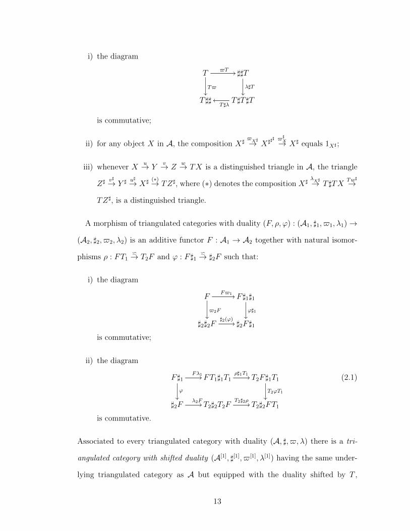
i) the diagram

T$T //

T$��

]]T

λ]T��

T]] T ]T ]TT]λoo

is commutative;

ii) for any object X in A, the composition X]$X]→ X]]

] $]X→ X] equals 1X] ;

iii) whenever Xu→ Y

v→ Zw→ TX is a distinguished triangle in A, the triangle

Z] v]→ Y ] u]→ X] (∗)→ TZ], where (∗) denotes the composition X]λX]→ T]TX

Tw]→

TZ], is a distinguished triangle.

A morphism of triangulated categories with duality (F, ρ, ϕ) : (A1, ]1, $1, λ1)→

(A2, ]2, $2, λ2) is an additive functor F : A1 → A2 together with natural isomor-

phisms ρ : FT1w→ T2F and ϕ : F]1

w→ ]2F such that:

i) the diagram

FF$1 //

$2F��

F]1]1

ϕ]1��

]2]2F]2(ϕ)

// ]2F]1

is commutative;

ii) the diagram

F]1Fλ1//

ϕ

��

FT1]1T1ρ]1T1

// T2F]1T1

T2ϕT1��

]2Fλ2F// T2]2T2F

T2]2ρ// T2]2FT1

(2.1)

is commutative.

Associated to every triangulated category with duality (A, ],$, λ) there is a tri-

angulated category with shifted duality (A[1], ][1], $[1], λ[1]) having the same under-

lying triangulated category as A but equipped with the duality shifted by T ,

13

that is, ][1] := T], $[1] := −λ] ◦ $, λ[1] := −Tλ. Similarly, we may shift in

the other direction to obtain the shifted duality (A[−1], ][−1], $[−1], λ[−1]), where

][−1] := ]T ,$[−1] := (λ])−1 ◦ $, λ[−1] := −λT . Continuing in this manner, we ob-

tain, for every n ∈ Z, a triangulated category with duality (A[n], ][n], $[n], λ[n]).

A morphism of triangulated categories (F, ρ, ϕ) induces a morphism of the asso-

ciated triangulated categories with shifted dualities, e.g. we obtain a morphism

(F, ρ, ϕ[1]) of the triangulated categories with the duality shifted by T by defining

ϕ[1] := Tϕ ◦ ρ].

Definition 2.2. Let (A, ],$, λ) be a triangulated category with duality. A sym-

metric form is a pair (X, υ), where X is an object in A and υ : X → X] is a

morphism in A such that υ] ◦$ = υ. When υ is an isomorphism in A, the (X, υ)

is said to be a symmetric space. A symmetric form with respect to the shifted

duality ][n] will be called an A[n]-symmetric form, e.g. a A[−1]-symmetric form is

a pair (X, υ) with υ : X → (TX)] a morphism in A such that T (υ]) ◦ $[−1]X = υ

($[−1]X = (λ])−1 ◦ $, see Definition 2.1), and when the morphism defining the

symmetric form is an isomorphism in A we say it is an A[n]-symmetric space.

Given two symmetric spaces (X, υ) and (Y, φ): the orthogonal sum is defined

to be the symmetric space (X, υ) ⊥ (Y, φ) :=

(X ⊕ Y,

(υ 00 φ

)); an isometry

h : (X, υ)w→ (Y, φ) is an isomorphism h : X

w→ Y in A such that h]φh = υ; (X, υ)

and (Y, φ) are said to be isometric if there exists an isometry between them.

Proposition 2.3. [6, Theorem 1.6] Let (A, ],$, λ) be a triangulated category with

duality such that 12∈ A. Let (X, υ) be a A[−1]-symmetric space (see Definition

2.2). Choose a distinguished triangle Xυ→ (TX)]

u1→ Cu2→ TX over υ in A. Then,

there exists an isomorphism ψ : Cw→ C] in A defining a symmetric space (C,ψ)

14

in (A, ],$, λ) and a commutative diagram

X υ //

$[−1]X

��

(TX)]

1��

u1 // C

ψ��

u2 // TX

T$[−1]X

��

]T ]TXT (υ])

// (TX)]u]2 // C]

λ]◦u]1// T]T ]TX

(2.2)

in which the rows are distinguished triangles. If we choose another distinguished

triangle Xυ→ (TX)]

u′1→ C

′ u′2→ TX over υ and another isomorphism ψ

′defining a

symmetric space (C′, ψ) such that the resulting diagram 2.2 is commutative, then

the symmetric spaces (C′, ψ′) and (C,ψ) are isometric.

Definition 2.4. Let (A, ],$, λ) be a triangulated category with duality such that

12∈ A. The isometry class of the symmetric space (C,ψ) from Proposition 2.3 is

called the cone of the A[−1]-symmetric form υ : X → (TX)]. A symmetric space in

(A, ],$, λ) which is equal to a cone is called a metabolic space (aka neutral space)

space in (A, ],$, λ).

Definition 2.5. Let (A, ],$, λ) be a triangulated category with duality such that

12∈ A. The Witt group W 0(A) is the free abelian group generated by isometry

classes of symmetric spaces in (A, ],$, λ) modulo the metabolic spaces and the

relations [X ⊥ Y ] = [X] + [Y ] (or equivalently, the Grothendieck-group of the

abelian monoid of isometry classes of symmetric spaces modulo the metabolic

spaces). For every n ∈ Z, the shifted Witt group W n(A) is defined to be W 0(A[n]),

in other words, it is the Witt group of the triangulated category with duality

(A[n], ][n], $[n], λ[n]).

Proposition 2.6. [6, Proposition 1.14] Let (A, ],$, λ) be a triangulated category

with duality. For every n ∈ Z, there is an isomorphism of triangulated categories

with duality A[n] w A[n+4] which induces an isomorphism of triangulated Witt

groups W n(A) w W n+4(A).

15

Proposition 2.7. [9, Theorem 1.4.14] Let (A, ],$, λ) be a triangulated category

with duality such that 12∈ A. Let

A0 → A→ S−1A (2.3)

be a short exact sequence of triangulated categories with duality, that is, A → S−1A

is a localization with respect to a class S of morphisms in A, and A0 is the full

subcategory of A consisting of objects which become isomorphic to zero in S−1A,

and the dualities on A0 and S−1A are induced from the duality on A. Then, the

short exact sequence 2.3 induces a long exact sequence of abelian groups

· · · → W n(A0)→ W n(A)→ W n(S−1A)→ · · · (2.4)

2.2.1 The Derived and Coherent Witt Groups of Schemes

Now we will give an important example of a triangulated category with duality.

2.8. Let (E , ]) be an exact category with duality ].The homotopy category Kb(E)

of bounded chain complexes in E is a triangulated category having as objects

bounded chain complexes in E and as morphisms the chain maps up to chain

homotopy. The bounded derived category Db(E) is obtained from the homotopy

category by formally inverting quasi-isomorphisms. The duality ] on E induces a

duality on the homotopy category Kb(E) and on the derived category Db(E). Let

$ denote the isomorphism to the double dual $ : 1w→ ]] in Db(E) that is induced

from the canonical one in E . Then, (Db(E), ],$, 1) is a triangulated category with

duality. For a reference for these facts see [62, Section 3.1.3],[7, Section 2.6].

In particular, from 2.8 we have the following.

Definition 2.9. Let X be a scheme with 2 invertible in the global sections OX(X).

Let Vect(X) denote the exact category of vector bundles on X, that is, the cate-

gory of OX-modules which are locally free and of finite rank. For any vector bundle

16

E on X, the usual duality E ] := HomVect(X)(E ,OX) defines a duality on Vect(X).

Then, (Db(Vect(X)), ],$, 1) is a triangulated category with duality (2.8) with

12∈ Db(Vect(X)). The (derived) Witt groups of X are defined to be the trian-

gulated Witt groups W n(Db(Vect(X))) of the triangulated category with duality

(Db(Vect(X)), ],$, 1), and are denoted by W n(X).

As mentioned earlier, there is the following identification.

Proposition 2.10. [9, Theorem 1.4.11] Let X be a scheme with 2 invertible in

its global sections. Then W 0(X) is the Witt group W (X) as defined by Knebusch.

In particular, when X = Spec k, where k is field of characteristic not 2, then

W 0(Spec k) equals W (k) the classical Witt group of k.

The principal result on the derived Witt groups of local rings is the following

theorem of P. Balmer.

Proposition 2.11. [7, Theorem 5.6] Let A be a local ring in which 2 is invertible.

Then, among the derived Witt groups of A, we have W 1(A) = 0,W 2(A) = 0, and

W 3(A) = 0. That is, there is only one non-trivial Witt group, namely W 0(A) '

W (A). This holds in particular for fields of characteristic not 2.

Next we recall the definition of the coherent Witt groups.

Definition 2.12. Let X be a noetherian scheme with 2 invertible in its global

sections. Let M(X) denote the category of OX-modules, and let Dbcoh(X) denote

the full subcategory of the bounded derived category Db(M(X)) consisting of

complexes having coherent homology. A dualizing complex for X is defined to

be a bounded complex K of injective coherent sheaves with the property that

the natural morphism of complexes ωK (essentially the evaluation map, see [30,

§1.6] for a precise description) from an object M of Dbcoh(X) to its double dual

17

HomOX (HomOX (M,K), K) is an isomorphism (in Dbcoh(X)). The coherent Witt

groups of X are defined to be the triangulated Witt groups of the triangulated

category with duality (Dbcoh(X),HomOX (−, K), ωK , 1) (2.5), and are denoted by

W n(X,K).

Remark 2.13. Let X be a noetherian scheme with 2 invertible in its global sec-

tions.

(a) When X is regular, any injective resolution I• of OX yields a dualizing

complex, and the quasi-isomorphism OX'→ I• induces an isomorphism

W n(X)'→ W n(X, I•) from the derived Witt groups to the coherent Witt

groups [30, Example 2.4]. However, this isomorphism is not functorial.

(b) Every dualizing complex I• for X yields a codimension function µI : X → Z

[30, Lemma 1.12 and following discussion]. When X is regular and the dual-

izing complex is given by an injective resolution of the structure sheaf, this

function is exactly the usual codimension function x 7→ codim(x) [30, Exam-

ple 1.13].

2.3 The Gersten Complex for the Witt Groups

We construct the Gersten complex for the Witt groups and then identify it with

the ‘usual’ Gersten complex. Even though we work with regular schemes, we use

the coherent Witt groups to construct the Gersten complex for two reasons: one is

that in we use results of S. Gille on the differentials of the Gersten complex that is

defined in terms of coherent Witt groups in Chapter 2.4; the other is that we use

the transfer for the coherent Witt groups for an argument involving the Gersten

complex in Chapter 3.3.

18

2.3.1 Construction

Let X be a noetherian regular Z[12]-scheme of dimension d, and let I• denote

the dualizing complex obtained by taking an injective resolution of the structure

sheaf OX (Remark 2.13 (a)). We will denote the coherent Witt groups of X with

coefficients in I• by W (X, I•). We briefly recall the well-known construction of the

coniveau spectral sequence for coherent Witt groups [30, §5.8]. For any OX-module

M , we denote by suppM the set of points x ∈ X for which the localization Mx is

non-zero. For any complex M• ∈ Dbc(X), suppHi(M•) is a closed subscheme of X

since Hi(M•) is coherent [34, corollary 7.31]. Then

suppM• :=⋃i∈Z

suppHi(M•)

is also a closed subspace of X as it is a finite union of closed subspaces. Recall that

the codimension codimX(Z) of a closed subspace Z of X is defined as

codim(Z) = infη∈ZdimOX,η

where the infimum runs over the generic points η ∈ Z of Z.

For any integer q ≥ 0, let Dq(X) ⊂ Dbc(X), or simply Dq, consist of those

complexes having codimension of support greater than or equal to q, that is

Dq(X) = {M• ∈ Dbc(X)|codimX(suppM•) ≥ q} (2.5)

For q ≥ 0, we have short exact sequences [29, Section 3.3] of triangulated cate-

gories with duality

Dq+1 → Dq → Dq/Dq+1 (2.6)

so we obtain from Balmer’s localization theorem (Proposition 2.7) the long exact

sequence

· · · → W p(Dq+1)ip,q+1→ W p(Dq)

jp,q→ W p(Dq/Dq+1)kp,q→ · · · (2.7)

19

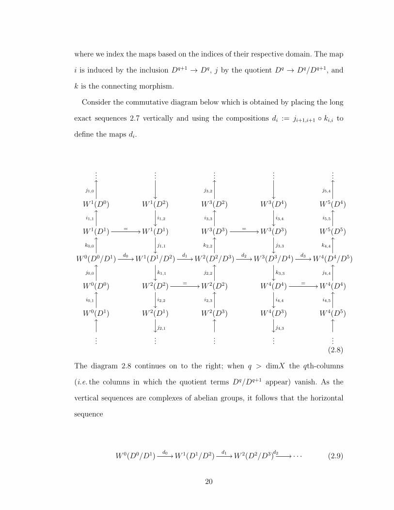
where we index the maps based on the indices of their respective domain. The map

i is induced by the inclusion Dq+1 → Dq, j by the quotient Dq → Dq/Dq+1, and

k is the connecting morphism.

Consider the commutative diagram below which is obtained by placing the long

exact sequences 2.7 vertically and using the compositions di := ji+1,i+1 ◦ ki,i to

define the maps di.

......

��

......

��

...

W 1(D0)

j1,0

OO

W 1(D2)

i1,2��

W 3(D2)

j3,2

OO

W 3(D4)

i3,4��

W 5(D4)

j5,4

OO

W 1(D1)

i1,1

OO

= //W 1(D1)

j1,1��

W 3(D3)

i3,3

OO

= //W 3(D3)

j3,3��

W 5(D5)

i5,5

OO

W 0(D0/D1)

k0,0

OO

d0 //W 1(D1/D2)

k1,1��

d1 //W 2(D2/D3)

k2,2

OO

d2 //W 3(D3/D4)

k3,3��

d3 //W 4(D4/D5)

k4,4

OO

W 0(D0)

j0,0

OO

W 2(D2)

i2,2��

= //W 2(D2)

j2,2

OO

W 4(D4)

i4,4��

= //W 4(D4)

j4,4

OO

W 0(D1)

i0,1

OO

W 2(D1)

j2,1��

W 2(D3)

i2,3

OO

W 4(D3)

j4,3��

W 4(D5)

i4,5

OO

...

OO

......

OO

......

OO

(2.8)

The diagram 2.8 continues on to the right; when q > dimX the qth-columns

(i.e. the columns in which the quotient terms Dq/Dq+1 appear) vanish. As the

vertical sequences are complexes of abelian groups, it follows that the horizontal

sequence

W 0(D0/D1)d0 //W 1(D1/D2)

d1 //W 2(D2/D3)d2 // · · · (2.9)

20

is a complex of abelian groups. When X is finite dimensional of dimension d, the

complex (2.9) becomes the complex

W 0(D0/D1)d0 //W 1(D1/D2)

d1 // · · ·dd−1//W d(Dd) // 0 (2.10)

where we have identified W d(Dd/Dd+1) = W d(Dd).

AsW 0(D0) = W (X), the complex (2.10) augmented by the map j0,0 : W 0(D0)→

W 0(D0/D1) determines a complex

0 // W (X)j0,0//W 0(D0/D1)

d0 //W 1(D1/D2)d1 // · · ·

dd−1//W d(Dd) // 0.

(2.11)

Remark 2.14. If we use the derived Witt groups instead of the coherent Witt

groups in the above construction of the Gersten complex 2.10 by using the codi-

mension of support filtration on the bounded derived category of vector bundles

Db(Vect(X)) on X, then this results in the complex

0 //W (X)j0,0//W 0(D0/D1)

d0 //W 1(D1/D2)d1 // · · ·

dd−1//W d(Dd) // 0

(2.12)

begining with the derived Witt group W (X) of X. However, the complex 2.12 and

the complex 2.11 are isomorphic kjhsdafkjh kj[10, Section 3, Another Construc-

tion], where the isomorphism is induced by the quasi-isomorphism OX'→ I•.

Definition 2.15. Let X be a noetherian regular Z[12]-scheme of dimension d.

We index the complex 2.10 cohomologically by setting the degree p term to be

W p(Dp/Dp+1). The complex 2.10 will be denoted by Ger(X), and called the Ger-

sten complex for the Witt groups of X, or simply the Gersten-Witt complex of

X. Following Remark 2.14, the complexes 2.12 and 2.11 will both be called the

augmented Gersten complex for the Witt groups of X since they are isomorphic.

21

Definition 2.16. Let A be a regular local ring. If the augmented Gersten complex

2.11 for the Witt groups of A is an exact complex, then we will say that the Gersten

conjecture is true for the Witt groups of A.

The following lemma is well-known (e.g. [10, Lemma 4.2]).

Lemma 2.17. Let X be a noetherian regular Z[12]-scheme of dimension d. The Witt

sheaf W is the Zariski sheaf on X that is associated to the presheaf U 7→ W (U)

on X. If, for all x ∈ X, the Gersten conjecture (see definition 2.16) is true for the

Witt groups of OX,x, then, for all p ≥ 0, Hp(Ger(X)) = HpZar(X,W), that is, the

cohomology of the Gersten complex agrees with the Zariski cohomology of X with

coefficients in W.

Next, a simple diagram chase lemma which is well-known.

Lemma 2.18. Let X be a noetherian regular Z[12]-scheme. Then we have the fol-

lowing:

(i) If the morphism i0,1 : W 0(D1)→ W 0(D0) (from the long exact sequence 2.7)

is zero, then the augmented Gersten complex is exact at W (X);

(ii) If the morphism i1,2 : W 1(D2) → W 1(D1) is zero, then the augmented Ger-

sten complex is exact at W 0(D0/D1);

(iii) Let p > 0 be an integer. If the morphisms ip,p : W p(Dp)→ W p(Dp−1), ip+1,p+2 :

W p+1(Dp+2) → W p+1(Dp+1) (2.7) are both zero, then the Gersten complex

for the Witt groups (2.15) is exact in degree p.

In particular, if, for all p, q ∈ Z, the maps ip,q : W p(Dq) → W p(Dq−1) are zero,

then the augmented Gersten complex (2.11) is exact.

22

Proof. To prove (i), consider the diagram (2.8). In view of the exactness of the

vertical sequences we see that if W 0(D1)i0,1→ W 0(D0) is zero, then W 0(D0)

j0,0→

W 0(D0/D1) is injective. Similarly, to prove (ii) note that if W 1(D2)i1,2→ W 1(D1) is

zero, then W 1(D1)j1,1→ W 1(D1/D2) is injective. Hence, the kernel of the differential

d0 = j1,1 ◦ k0,0 equals the kernel of k0,0, which is W (X) the image of j0,0. So the

augmented Gersten complex (2.11) is exact in degree 0.

To prove (iii) we have the following in any positive degree p: if ip,p = 0, then

kp−1,p−1 is surjective, so the image of the differential dp−1 is the image of jp,p; if

ip+1,p+2 = 0, then jp+1,p+1 is injective, so the kernel of the differential dp is the

kernel of kp,p. Hence, if ip+1,p+2 = ip,p = 0, then the Gersten complex for the Witt

groups is exact in degree p. The final statement of the Lemma immediately follows

from (i), (ii) and (iii).

Lemma 2.19. [10, Lemma 3.3 and Section 4] Let A be a regular local ring and

f ∈ A a regular parameter. Then there is a short exact sequence of complexes

0→ Ger(A/f)[−1]→ Ger(A)→ Ger(Af )→ 0 (2.13)

where Ger(A/f)[−1] denotes the shift to the right, so that the degree 0 part of this

complex is the degree -1 part of Ger(A/f), and in particular, H0(Ger(A/f)[−1]) =

0, and, for p ≥ 1, Hp(Ger(A/f)[−1]) = Hp−1(Ger(A/f)) . It follows that the long

exact sequence of cohomology groups

· · · → Hp(Ger(A/f)[−1])→ Hp(Ger(A))→ Hp(Ger(Af ))→ · · · (2.14)

which is determined by the short exact sequence 2.13 may be rewritten as the long

exact sequence

· · · → Hp−1(Ger(A/f))→ Hp(Ger(A))→ Hp(Ger(Af ))→ · · · (2.15)

23

2.3.2 Identification

In this section we recall some results which explicitly describe the Witt groups of

the quotient W p(Dq/Dq+1) and lead to a description of the Gersten complex in

terms of the Witt groups of the residue field. The following are all well-known.

Proposition 2.20. [26, c.f. Theorem 3.12] If X is a noetherian regular scheme,

then, for all q ≥ 0, there are equivalences of triangulated categories

Dq/Dq+1 '∐x∈Xq

Dbfl(M(OX,x)) (2.16)

where Dbfl(M(OX,x)) denotes those complexes of OX,x-modules in Db

coh(M(OX,x))

whose homology has finite length and Xq denotes the set of points x ∈ X having

dimOX,x = q.

The Witt groups of the triangulated categories Dbfl(M(OX,x) are described in

the next Lemma.

Proposition 2.21. [26, c.f. Theorem 3.10 and Corollary 3.11] Let O be a regular

local ring with residue field k such that chark 6= 2. Then W n(Dbfl(M(O))) ' W (k)

if n = dim O mod 4, and W n(Dbfl(M(O))) = 0 otherwise.

Taking the Witt groups of both sides of the equivalence 2.16 given in the state-

ment of Proposition 2.20 and applying Proposition 2.21 one obtains the next propo-

sition.

Proposition 2.22. [26, c.f. Theorem 3.14] Let X be a noetherian regular Z[12]-

scheme of finite Krull dimension, and let 0 ≤ q ≤ dimX be an integer. For any

p ∈ Z, the Witt groups W p+q(Dq/Dq+1) of the quotients Dq/Dq+1 vanish when

p+ q 6= q mod 4, and are otherwise, when p+ q = q mod 4,

W p+q(Dq/Dq+1) ' W q(Dq/Dq+1) '⊕x∈Xq

W (k(x)) (2.17)

24

where the isomorphism on the left is induced by the 4-periodicity (Proposition 2.6),

and the isomorphism on the right is the composition of the isomorphism induced by

the equivalence of triangulated categories 2.16 given in the statement of Proposition

2.20) followed by the isomorphism of Proposition 2.21 (x ∈ Xq means by definition

that dimOX,x = q).

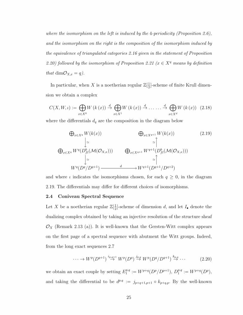
In particular, when X is a noetherian regular Z[12]-scheme of finite Krull dimen-

sion we obtain a complex

C(X,W, ι) :=⊕x∈X0

W (k (x))d→⊕x∈X1

W (k (x))d→ . . . . . .

d→⊕x∈Xd

W (k (x)) (2.18)

where the differentials dq are the composition in the diagram below

⊕x∈Xq W (k(x))

'��

⊕x∈Xq+1 W (k(x))

⊕x∈Xq W q(Db

fl(M(OX,x)))

'��

⊕x∈Xq+1 W q+1(Db

fl(M(OX,x)))

'

OO

W q(Dq/Dq+1) d //W q+1(Dq+1/Dq+2)

'OO

(2.19)

and where ι indicates the isomorphisms chosen, for each q ≥ 0, in the diagram

2.19. The differentials may differ for different choices of isomorphisms.

2.4 Coniveau Spectral Sequence

Let X be a noetherian regular Z[12]-scheme of dimension d, and let I• denote the

dualizing complex obtained by taking an injective resolution of the structure sheaf

OX (Remark 2.13 (a)). It is well-known that the Gersten-Witt complex appears

on the first page of a spectral sequence with abutment the Witt groups. Indeed,

from the long exact sequences 2.7

· · · → W p(Dq+1)ip,q+1→ W p(Dq)

jp,q→ W p(Dq/Dq+1)kp,q→ · · · (2.20)

we obtain an exact couple by setting Ep,q1 := W p+q(Dp/Dp+1), Dp,q

1 := W p+q(Dp),

and taking the differential to be dp,q := jp+q+1,p+1 ◦ kp+q,p. By the well-known

25

method of Massey’s exact couples, this exact couple determines a cohomological

spectral sequence with abutment the coherent Witt groups. However, had we used

to codimension of support filtration on the bounded derived category of vector

bundles the resulting spectral sequence would be isomorphic [10, Section 3, Another

Construction]. Therefore, we obtain the spectral sequence below

Ep,q1 := W p+q(Dp/Dp+1)⇒ W p+q(X) (2.21)

converging to the derived Witt groups of X. The differential dr on the r-th page of

this spectral sequence has bidegree (r, 1−r). SinceX is finite dimensional, this spec-

tral sequence is bounded, hence converges. Furthermore, recalling the construction

of the Gersten complex for the Witt groups 2.10, we have that Ger(X) = E∗,01 by

construction. Next, using Proposition 2.22 to identify the Witt groups of the quo-

tients, we have that the groups Ep,q1 appearing on the E1-page, vanish for p+q 6= p

mod 4, and that they takes the form

Ep,q1 =

⊕x∈Xp

W (k(x))

when q is congruent to 0 mod 4.

One well-known general fact about the shifted Witt groups of arithmetic schemes

is the following easy corollary to the coniveau spectral sequence that was alluded

to in the introduction.

Corollary 2.23. Let X be a noetherian regular Z[12]-scheme of Krull dimension

d. If no residue field of X is formally real (a field is formally real if and only if −1

is not a sum of squares), then the Witt groups W n(X) are torsion groups.

Proof. As no residue field of X is formally real, for each x ∈ X, the Witt group

of the residue field W (k(x)) is a torsion group [59, Theorem 6.4 (ii)]. As arbitrary

direct sums of torsion abelian groups are torsion, from the description in Equation

26

2.4 of the groups on the first page of coniveau spectral sequence, we have that

all the groups appearing on the first page are torsion groups. Since X is finite

dimensional, the first page of the spectral sequence is bounded, hence convergent,

so we have that the Witt groups are torsion.

The next result we use in Chapter 3.3.

Corollary 2.24. Let X = SpecA be a regular local ring with 12∈ A. If the Gersten

complex Ger(X) (Definition 2.15) is exact in degrees greater than or equal to 4,

then the Gersten conjecture is true for the Witt groups of A (Definition 2.16).

Proof. The hypothesis on the Gersten complex is equivalent to Ep,02 = 0 for all

p ≥ 4. Since the differential has bidegree (r, 1 − r), it follows that the coniveau

spectral sequence collapses on the E2-page, and that W 0(A) = E0,02 , W 1(A) = E1,0

2 ,

W 2(A) = E2,02 ,W 3(A) = E3,0

2 . However, as the derived Witt groupsW 1(A),W 2(A),W 3(A)

are all zero (Proposition 2.11), this proves that Ep,01 = 0 for all p ≥ 1, and that

E0,01 = W 0(A), proving the lemma.

27

The Finite Generation Question

3.1 Kato Complexes, Kato Cohomology, and Motivic Cohomology

For a very general class of schemes K. Kato [43, §1] introduced complexes that gen-

eralized to higher dimensions classical exact sequences for Galois cohomology. He

made some conjectures on their exactness in various situations. In this section, we

recall some finiteness results about their cohomology that are easily obtained using

finiteness of etale cohomology, and we explain their relation to motivic cohomology.

3.1.1 Kato Complexes

First a remark about the implications of assuming 2 is invertible.

Remark 3.1. Recall that when X is a scheme, we say that 2 is invertible on X

when 2 is a unit in the global sections Γ(X,OX).

(a) When X is of finite type over Z, saying that 2 is invertible on X is the same

as saying that X is of finite type over Z[12]. Furthermore, when X is of finite

type over Fp (p > 2), it follows that 2 is invertible on X and that X is of

finite type over Z (as Fp is of finite type over Z, and compositions of finite

type morphisms are of finite type), hence X is of finite type over Z[12].

(b) From the assumption 2 is invertible on X, it also follows that each residue

field k(x) of X has characteristic different from 2, and that there is an isomor-

phism of Gal(k(x)s|k(x))-modules Z/2Z ' µ2 := {a ∈ k(x)s|a2 = 1}, where

k(x)s denotes a separable closure of k(x).

(c) When 2 is invertible on X, in the global sections −1 6= 1, so −1 determines

an isomorphism of etale sheaves µ2 ' Z/2Z, hence µ⊗n2 is isomorphic Z/2Z.

Recall that on a scheme X, isomorphisms between the etale sheaf µ2 and the

28

constant sheaf Z/2Z correspond to global sections of X which have order 2

on each connected component [66, see p. 100 for definitions and details].

Next, we recall what we mean by the residue and corestriction maps.

Definition 3.2. Let A be a discrete valuation ring (DVR) with fraction field K

and residue field k. Assume that char(k) 6= 2. By the residue homomorphism for

A, we mean the group homomorphism from the Galois cohomology of K to the

Galois cohomology of the residue field k

∂n : HnGal (K,Z/2Z)→ Hn−1

Gal (k,Z/2Z) ,

as defined in [43, p. 149]. Note that this is the same as the definition given in [3,

p. 475]. When n = 0, we set Hn−1 (k,Z/2Z) = 0.

Definition 3.3. Let F be a finite extension of a field L. By the corestriction

homomorphism for the finite extension L/K, we mean the group homomorphism

corL/K : HnGal (L,Z/2Z)→ Hn

Gal (K,Z/2Z) ,

as defined in [3, p. 471]. This agrees with the definition used by K. Kato in [43].

Recall that a locally noetherian scheme X is said to be excellent [38, Definition

7.8.5] if for some covering of X by affine schemes Uα =Spec(Aα), each of the rings

Aα are excellent [38, Definition 7.8.2].

The next example is important for understanding the definition of the differen-

tials in the Kato complex.

Example 3.4. Let X be a noetherian excellent scheme, let y ∈ X be a point

of X, and let Z := {y} denote the reduced closed subscheme with underlying

topological space {y}. Since X is excellent, every locally finite-type X-scheme X′

is excellent [38, Proposition 7.8.6]. In particular, via the closed immersion Z → X,

29

Z is excellent. Therefore, Z is an integral excellent scheme. For an integral excellent

ring A, its integral closure in Frac(A) is a finite A-algebra [38, Scholie 7.8.3]. It

follows that the normalization morphism Z′ → Z is finite [48, Theorem 2.39 (d)].

In particular, the normalization is quasi-finite, so the fiber over any point x ∈ Z

has only finitely many points x1, . . . , xn and for each of the xi the field extension

k (xi) /k (x) is a finite extension.

Definition 3.5. Let X be a scheme. Recall that the dimension of a point x ∈ X is

defined to be the (combinatorial) dimension dim(x) := dim({x}) of the topological

space defined by the closure of x. The set of dimension p points of X is denoted

by Xp. The codimension of a point x ∈ X is defined to be the Krull dimension

codim(x):=dim(OX,x) of the local ring of X at the point x ∈ X. This is equal to

the topological codimension of the closed subspace {x} in X [38, Proposition 5.12].

The set of codimension p points of X will be denoted by Xp.

Definition 3.6 (The yx-component ∂yx of the differential). Let X be a noetherian

excellent scheme with 2 invertible. Recall the facts of Example 3.4. Let x ∈ Xp+1

and y ∈ Xp such that x ∈ {y}. Let Z := {y} denote the reduced closed subscheme

with underlying topological space {y}. Let Z′ → Z be the normalization of Z. The

field extensions k (xi) /k (x) for each of the finitely many points x1, . . . , xn ∈ Z′

ly-

ing over x ∈ Z are finite extensions, so for all non-negative integers j ∈ Z, there are

well-defined corestriction maps (Definition 3.3) cork(xi)/k(x) : Hj (k (xi) ,Z/2Z) →

Hj (k (x) ,Z/2Z). Each xi ∈ Z′

is of codimension 1 in Z′

(use the dimension for-

mula [49, Theorem 15.6] together with the fact that the extension k (xi) /k (x) is

finite, hence of transcendence degree 0). So the localization OZ′ ,xi of the normal-

ization at the point xi is a DVR, with fraction field k (y) and residue field k (xi).

30

Hence, each xi defines residue homomorphisms (Definition 3.2)

∂xi : HjGal (k (y) ,Z/2Z)→ Hj−1

Gal (k (xi) ,Z/2Z)

for all non-negative integers j ∈ Z. The yx-component dyx is defined ( c.f. [41,

§0.6]) as

dyx :=∑xi|x

cork(xi)/k(x) ◦ ∂xi ,

where the sum is taken over the finitely many points xi ∈ Z′

lying over x.

Definition 3.7 (Cohomological Kato complexes). Let X be a noetherian excellent

scheme, finite dimensional of dimension d. We assume that 2 is invertible on X

(this is not necessary for the definition in general). It follows from this assumption

that for every n ≥ 0 the Tate twist µ⊗n2 is isomorphic to the constant sheaf Z/2Z

(see Remark 3.1 (b)). The n-th Kato complex is defined to be the complex

C(X,Hn) :=⊕x∈X0

Hn(k(x),Z/2Z)→⊕x∈X1

Hn−1(k(x),Z/2Z)→ · · ·

· · · →⊕x∈Xd

Hn−d(k(x),Z/2Z),

where k (x) denotes the residue field of a point x ∈ X, and we setHm(k(x),Z/2Z) =

0 for m < 0. Kato complexes are often indexed homologically, but here we will

always use cohomological indexing by placing the term summing over the codi-

mension p points in degree p. The m-th cohomology of the n-th Kato complex

C(X,Hn) will be denoted by Hm(C(X,Hn)). The differential is defined compo-

nentwise. The yx-component ∂yxi : H i (k (y) ,Z/2Z) → H i−1 (k (x) ,Z/2Z) of the

i-th differential is defined as follows: If x /∈ {y}, then set dyx = 0. If x ∈ {y}, then

dyx is defined as in Definition 3.6.

Remark 3.8. When X is a variety over a field, by definition the Kato complexes

are the same as Rost’s cycle complexes for the cycle module defined by Galois

31

cohomology [58, see §2.10 for the definition of the differential, as well as Remark

(2.5)].

Finally, we recall some conditions under which the dimension can be replaced

by the codimension in the definition of the Kato complexes.

Definition 3.9. Let X be a scheme. The scheme X is said to be biequidimen-

sional [37, §14 p. 11] if it is finite dimensional, equidimensional (aka pure, i.e. the

dimension of each irreducible component is the same), equicodimensional (the codi-

mension of each minimal closed irreducible set in X is the same), and catenary

(see [37, §14 p. 11]).

Lemma 3.10 (Corollaire 14.3.5 EGA IV Premiere Partie). For any noetherian

biequidimensional scheme X of dimension d and for any point x ∈ X, the dimen-

sion and codimension of x are related as follows: dim(x) = d− codim(x). That is

for any p, the set of dimension p points of X is equal to the set of codimension

d− p points Xp = Xd−p.

Remark 3.11. There are examples of finite dimensional schemes which are regu-

lar (hence catenary) and integral (hence equidimensional) possessing points x for

which dim(x) + codim(x) is not equal to the dimension of the scheme [38, Remark

5.2.5(i)]. However, when X is a variety over a field, pure of dimension d, it is

biequidimensional [38, follows from Proposition 5.2.1].

3.1.2 Relation to Etale Cohomology

Jannsen, Saito, and Sato showed that for very general schemes, the Kato complexes

appear on the first page of the etale niveau spectral sequence. As we restate their

result slightly to suit our purposes, we recall briefly their proof.

Proposition 3.12. (See [41, Section 1.5 and Theorem 1.5.3].) Let X be a noethe-

rian regular excellent Z[12]-scheme, pure of dimension d. Filtering by codimension

32

of support gives a convergent spectral sequence

Ep,q1 (X,Z/2Z) :=

⊕x∈Xp

Hq−pet (k (x) ,Z/2Z) =⇒ Hp+q

et (X,Z/2Z),

with differential dr of bidegree (r, 1− r). Furthermore, the complexes appearing on

the first page of the spectral sequence E1∗,q (X,Z/2Z) agree up to signs with the

Kato complexes C(X,Hq), hence the second page of the spectral sequence consists

of Kato cohomology Ep,q2 = Hp(C(X,Hq)).

Proof. For any noetherian scheme, pure of dimension d, one may construct a co-

homological spectral sequence of the form (e.g. , [17, Section 1])

Ep,q1 (X,Z/2Z) :=

⊕x∈Xp

Hp+qx (X,Z/2Z) =⇒ Hp+q

et (X,Z/2Z).

where Hp+qx (X,Z/2Z) is defined to be the colimit, over all non-empty open sub-

subsets U ⊂ X containing x, of the groups Hp+q

{x}∩U(U,Z/2Z). Since X, and hence

{x}, is excellent, there exists an open U0 ⊂ X such that {x} ∩ U is regular for

U ⊂ U0. In this situation, if x ∈ Xp, then {x} ∩ U is a codimension p embedding

in U , hence by absolute purity [22, Theorem 2.1]

Hp+q−2pet

({x} ∩ U,Z/2Z

)' Hp+q

{x}∩U(U,Z/2Z)

so it follows that

Ep,q1 (X,Z/2Z) '

⊕x∈Xp

Hq−pet (k (x) ,Z/2Z)

For any y ∈ Xp, x ∈ Xp+1, the yx-components of the differentials

Hq−pet (k (y) ,Z/2Z)→ Hq−p−1

et (k (x) ,Z/2Z)

commute, up to signs, with those of the Kato complex [41, Theorem 1.1.1]. This

completes the proof.

33

Corollary 3.13. Let X be a separated scheme that is smooth (i.e. formally smooth

and of finite type) over Z[12], pure of dimension d. The spectral sequence of Propo-

sition 3.12 takes the form

Ep,q2 (X,Z/2Z) = Hp

Zar(X,Hq) =⇒ Hp+q

et (X,Z/2Z),

where HpZar(X,Hq) denotes the Zariski cohomology of the Zariski sheaf Hq on X

associated to the presheaf U 7→ Hqet(U,Z/2Z). Hence, for all p, q ∈ Z the Kato

cohomology groups Hp(C(X,Hq)) and the Zariski cohomology groups HpZar(X,Hq)

agree.

Proof. To prove the corollary, it suffices to show that the sheaf of complexes as-

sociated to the presheaves U 7→ E∗,q1 (U,Z/2Z) is a flasque resolution of Hq. A

complex of sheaves is exact if and only if it is exact on stalks. So, it suffices to

demonstrate that, for every point x ∈ X, the complex E∗,q1 (OX,x,Z/2Z) is exact

in positive degrees and in degree zero E20,q ' Hq

et(OX,x,Z/2Z). This is known as

the Gersten conjecture. Since the morphism X → Spec(Z[12]) is smooth, the local

ring OX,x is formally smooth and essentially of finite type over OZ[ 12

],y. The ring

OZ[ 12

],y is either a DVR or a field. In both cases, the Gersten conjecture is known.

For the field case see, for example [15], and in the DVR case it was proved by Gillet

[32].

Lemma 3.14. Let X be a smooth variety (i.e. separated, formally smooth and of

finite type) over a finite field Fp (p > 2), pure of dimension d. For any codimension

p point x ∈ Xp of X, we have cd2(k(x)) ≤ 1 + d− p, where cd2(k(x)) denotes the

etale cohomological 2-dimension of the residue field of x. Considering the E1 entries

of the coniveau spectral sequence, if q > d + 1, then Ep,q1 = 0 for all p ∈ Z, and

hence the Kato complex C(X,Hq) vanishes.

34

Proof. Let x ∈ Xp be a codimension p point of X. By [1, Expose X, Theorem

2.1] cd2(k(x)) ≤ 1 + tr.degFpk(x), where cd2(k(x)) denotes the etale cohomological

2-dimension of the residue field of k(x) of x. As X is of finite type over a field,

one has [38, Corollaire 5.2.3] that dimx(X) = dim(OX,x) + tr.degFpk(x). It results

from [37, Proposition 14.1.4] that d = dim(X) ≥ dimx(X) for all x ∈ X. Hence,

d−p ≥ tr.degFpk(x), proving that cd2(k(x)) ≤ 1+d−p. This proves the lemma.

3.1.3 Finiteness Results for Kato Cohomology

The Kato conjecture is the assertion of the next proposition. It was recently proved

by M. Kerz and S. Saito. We write it down for later reference.

Proposition 3.15. (See [45, Theorem 8.1]). Let X be a regular connected scheme

of Krull dimension d, proper over a finite field Fp (p > 2). The Kato cohomology

groups Hp(C(X,Hd+1)) vanish except when p = d, in which case Hd(C(X,Hd+1)) '

Z/2Z.

Next, recall the following fact about etale cohomology.

Lemma 3.16. Let X be a finite dimensional regular separated scheme of finite

type over Z[12]. In this situation, the etale cohomology groups Hm

et (X,Z/2Z) are

finite groups for all m ≥ 0.

Proof. Let f denote the structural morphism X → Spec(Z[12]). From the finiteness

theorem [18, Theoremes de Finitude, §1, Theorem 1.1] we have that, for all q ≥ 0,

the etale sheaves Rqf∗Z/2Z are constructible. Using the Leray spectral sequence

Ep,q1 = Hp

et(Z[12], Rqf∗Z/2Z) ⇒ Hp+q

et (X,Z/2Z) [18, Cohomologie etale, §2, p. 6],

we reduce to proving that the etale cohomology groups of Z[12] with coefficients in

a constructible sheaf are finite, which is known [50, Chapter 2, §3, Theorem 3.1

and following discussion].

35

Finally, we recall the following well known finiteness results for Kato cohomology,

which use the finiteness of etale cohomology together with the coniveau spectral

sequence.

Lemma 3.17 (Absolute finiteness). Let X be a pure regular separated scheme of

finite type over a base scheme S. Consider the following situations:

(a) dim(X) ≤ 1, and S = Spec(Z[12]).

(b) dim(X) ≤ 2, X is quasi-projective over S, and S = Spec(Fp) (p > 2).

(c) dim(X) = d, and S = Spec(Fp) (p > 2).

(d) dim(X) = d, X is quasi-projective, and S = Spec(Fp) (p > 2).

In situations (a) and (b), all the Kato cohomology groups of X are finite. In sit-

uation (c), the Kato cohomology group Hd(C(X,Hd+1)) is finite, and in situation

(d), the Kato cohomology group Hd(C(X,Hd)) is finite

Proof. In all situations, X satisfies the hypotheses of Lemma 3.16, hence the etale

cohomology of X is finite. Now consider the coniveau spectral sequence for etale

cohomology of Proposition 3.12. In situation (a), all differentials on the second page

of the spectral sequence are zero because dim(X) ≤ 1. So, the spectral sequence

collapses on the second page. Hence, as the abutment is finite (Lemma 3.16), the

Kato cohomology groups are finite.

For (b), using Lemma 3.14 we see that there is only one possibly non-zero dif-

ferential d2 : H0(C(X,H3)) → H2(C(X,H2)) on the second page of the spectral

sequence. It follows that all the other Kato cohomology groups appear on the sta-

ble page of the spectral sequence, hence are quotients of the induced filtration

on etale cohomology, so they are finite. The kernel and cokernel of d2 appear on

36

the stable page, hence are finite. Therefore H0(C(X,H3)) is finite if and only if

H2(C(X,H2)) is finite. The group H2(C(X,H2)), that is, E2,22 , is isomorphic to the

mod 2 Chow group CH2(X)/2 of codimension 2 cycles [15, Theorem 7.7], which

is finite for X quasi-projective over a finite field [45, Corollary 9.4(1)].

Now, assume we are in situation (c). From Lemma 3.14, it follows that the

differentials on the second page of the spectral sequence that are entering and

leaving the group Hd(C(X,Hd+1)) are zero. So, Hd(C(X,Hd+1)) appears on the

stable page, hence is finite since the abutment is finite.

Finally, assume we are in situation (d). As in the proof of case (b), the group

Ed,d2 = Hd(C(X,Hd)) is isomorphic to CHd(X)/2 [15, Theorem 7.7], hence is finite

for X quasi-projective over a finite field [45, Corollary 9.4(1)]. This completes the

proof of the lemma.

3.1.4 Relation to Motivic Cohomology

First recall the definition of the motivic cohomology of a smooth scheme over a

Dedekind domain. LetX be a scheme that is separated and smooth over a Dedekind

domain D. The standard algebraic m-simplex will be denoted by

4mD := Spec(D[t0, t1, . . . , tm]/Σit

i − 1)

and the free abelian group on closed integral subschemes of codimension n in

X ×D4mD , which intersect all faces properly, will be denoted by zn(X,m). Placing

zn(X, 2n − m) in degree m, the associated complex of presheaves is denoted by

Z(n), and we set Z/2Z(n) := Z(n) ⊗L Z/2Z. The complex Z/2Z(n) is in fact a

complex of sheaves for the etale topology [23, Lemma 3.1], and when considered

as a complex of sheaves for the Zariski topology it will be denoted by Z/2Z(n)Zar.

37

Definition 3.18. The motivic cohomology groups of X with mod 2 coefficients

Hmmot(X,Z/2Z(n)) are defined to be the hypercohomology groups of the complex

of Zariski sheaves Z/2Z(n)Zar.

Remark 3.19. In this remark we explain an observation of Totaro’s [67, Theorem

1.3 and surrounding discussion], that the Beilinson-Lichtenbaum conjecture leads

to the long exact sequence (3.2) below. Let X be a separated scheme that is smooth

over D := Z[12]. Let π : (Sm/D)et → (Sm/D)Zar denote the natural morphism of

sites.

(a) By the Beilinson-Lichtenbaum conjecture with Z/2Z-coefficients, we mean

that there is a quasi-isomorphism (Z/2Z(n))Zar ' τ≤nRπ∗Z/2Z of complexes

of Zariski sheaves on X. Recall that Rπ∗Z/2Z is the complex of Zariski

sheaves obtained by first taking an injective resolution I• of the etale sheaf

Z/2Z, from which we obtain an exact complex of etale sheaves. Then, ap-

ply π∗ to this complex to obtain a complex of Zariski sheaves (no longer

exact). The cohomology of this complex in degree i is the right derived

functor Riπ∗Z/2Z, which is isomorphic to the Zariski sheaf Hi associated

to the presheaf U 7→ H iet(X,Z/2Z) [66, I, Proposition 3.7.1]. The complex

τ≤nRπ∗Z/2Z is a complex of Zariski sheaves with cohomology in degree i

equal to Riπ∗Z/2Z when i ≤ n and zero otherwise. It follows that there is a

distinguished triangle in the derived category of Zariski sheaves on X

τ≤n−1Rπ∗Z/2Z→ τ≤nRπ∗Z/2Z→ Hn[−n] (3.1)

then from the associated long exact sequence in hypercohomology, if the

Beilinson-Lichtenbaum conjecture with Z/2Z-coefficients holds, we obtain

38

the long exact sequence ( c.f. [67, Theorem 10.3])

· · · → Hm+nmot (X,Z/2Z(n− 1))→ Hm+n

mot (X,Z/2Z(n))→ (3.2)

HmZar(X,Hn)→ Hm+n+1

mot (X,Z/2Z(n− 1))→ · · ·

where HmZar(X,Hn) denotes the Zariski cohomology of the Zariski sheaf Hn

associated to the presheaf U 7→ Hnet(U,Z/2Z).

(b) For smooth schemes over fields, the Beilinson-Lichtenbaum conjecture is

known, since it is equivalent to the Bloch-Kato conjecture [42, Theorem 19],

and the Bloch-Kato conjecture is known [42, see Theorem 21 and surrounding

discussion for an overview].

Lemma 3.20. Let X be a pure separated scheme that is smooth over Z[12]. Recall

that Hq denotes the Zariski sheaf associated to the presheaf U 7→ Hqet(U,Z/2Z).

Consider the following statements:

(a) The Zariski cohomology groups HpZar(X,Hq) are finite for all p, q ∈ Z;

(b) The motivic cohomology groups Hpmot(X,Z/2Z(q)) are finite for all p, q ∈ Z;

(c) The Beilinson-Lichtenbaum conjecture with Z/2Z-coefficients is true (see Re-

mark 3.19).

We have the implication (a) implies (b). Furthermore if we assume (c), then (a)

is equivalent to (b). Hence, by Corollary 3.13, (b) is equivalent to finiteness of the

Kato cohomology groups Hp(C(X,Hq)) for all p, q ∈ Z.

Proof. To prove that (a) implies (b), recall that there is a coniveau spectral se-

quence [23, see §4 for integral coefficients version]

Ep,q1 (X,Z/2Z(n)Zar) :=

⊕x∈Xp

H2n−p+qmot (k (x) ,Z/2Z(n− p)) =⇒ Hp+q

mot (X,Z/2Z(n),

39

and the sheaf of complexes associated to the presheaf U 7→ E∗,q1 (U,Z/2Z(n)Zar)

gives a flasque resolution of the sheaf Hq [23, Theorem 1.2 (2),(4) and (5), also see

remark at start of page 775], hence the Zariski cohomology groups HpZar(X,Hq)

are the only groups on the E2 page of the above spectral sequence, which converges

to the motivic cohomology groups, and it follows that (a) implies (b).

Now assume (c), from which we obtain the long exact sequence 3.2 (see Remark

3.19), from which it follows that (b) implies (a).

Next we recall some finiteness theorems relating the Kato cohomology to motivic

cohomology in the cases that finiteness of these groups is only partially known.

Lemma 3.21 (Relative finiteness). Let X be a pure separated scheme that is

smooth over a base scheme S. Consider the following situations:

(a) dim(X) ≤ 2, no residue field of X is formally real, S = Spec(Z[12]);

(b) dim(X) ≤ 3, X is connected and proper over S, and S = Spec(Fp) (p > 2);

(c) dim(X) ≤ 4, X is connected and proper over S, and S = Spec(Fp) (p > 2).

In situation (a):

(i) The groups H0Zar(X,H3), H0

Zar(X,H4), and H0Zar(X,H5) are finite if and

only if the groups H2Zar(X,H2), H2

Zar(X,H3), and H2Zar(X,H4) are finite.

Furthermore, all the other groups HpZar(X,Hq) are finite.

(ii) If all the groups H0Zar(X,H3), H0

Zar(X,H4), and H0Zar(X,H5) are finite, then

the motivic cohomology groups Hpmot(X,Z/2Z(p)) are finite for all p, q ∈

Z. Assuming the Beilinson-Lichtenbaum conjecture (see Remark 3.19 for an

explanation of what we mean by this), the converse is true.

In situation (b):

40

(i) The group H0Zar(X,H3) is finite if and only if the group H2

Zar(X,H2) is finite.

Furthermore, all the other cohomology groups HpZar(X,Hq) are finite.

(ii) The motivic cohomology groups Hpmot(X,Z/2Z(p)) are finite for all p, q ∈ Z

if and only if the group H0Zar(X,H3) is finite.

In situation (c):

(i) The groups H2Zar(X,H2), H2

Zar(X,H3), and H3Zar(X,H3) are finite if and

only if all the groups H0Zar(X,H3), H0

Zar(X,H4), and H1Zar(X,H4) are finite.

Furthermore, all the other groups HpZar(X,Hq) are finite.

(ii) The motivic cohomology groups Hpmot(X,Z/2Z(p)) are finite for all p, q ∈ Z

if and only if all the groups H0Zar(X,H3), H0

Zar(X,H4), and H1Zar(X,H4) are

finite.

Proof. In all situations, for (ii), finiteness of motivic cohomology implies finite-

ness of the Zariski cohomology groups by Lemma 3.20. Also, in each situation, to

prove (ii), it suffices to prove (i), for if groups named in (i) are finite then all the

groups HpZar(X,Hq) are finite, hence the motivic cohomology groups are finite by

Lemma 3.20. To prove (i), we work with the coniveau spectral sequence for etale

cohomology of Proposition 3.12.

First assume that we are in situation (a). The etale cohomological 2-dimension

of X is less than or equal to 2dim(X) + 1 [1, Expose 5, §6, Theorem 6.2], from

which it follows that whenever q > 2dim(X)+1, we obtain vanishing of the Zariski

sheaf Hq, and hence vanishing of HpZar(X,Hq). This, together with the fact that

dim(X) ≤ 2, gives that there are only three possibly non-zero differentials on

the second page of the spectral sequence, each having domain and codomain one

of the groups named in (i). This proves the second statement of (i). To prove

41

the first statement of (i), we prove finiteness of the kernel and cokernel of these

differentials. To prove this claim, observe that the kernel and cokernel of these

differentials appear on the third page of the spectral sequence, and the spectral

sequence collapses on the third page. As the abutment is finite (Lemma 3.16) this

proves the claim, finishing the proof of (i).

Assume that we are in situation (b). Then Lemma 3.14, Proposition 3.15, and

the fact that dim(X) ≤ 3, give that there is only one possible non-zero differential

on the second page of the spectral sequence. The domain of this differential is the

group H0Zar(X,H3). By the same argument used in the previous situation, this

differential has finite kernel and cokernel, which concludes the proof in situation

(b).

Finally, assume that we are in situation (c). Again, Lemma 3.14, Proposition

3.15, and the fact that dim(X) ≤ 4, give that there are only three possibly non-

zero differentials on the second page of the spectral sequence, each having domain

one of the groups named in the lemma. As before, the kernel and cokernel of these

differentials are finite. Hence, this concludes the proof in the case of situation

(c).

3.2 Arason’s Theorem

In this section, for an excellent scheme X with 2 invertible, we recall the definition

of the complex of abelian groups C(X, In). Arason essentially showed in [3] that if

the Bloch-Kato conjecture is true, then C(X, In) is isomorphic to the Kato complex

C(X,Hn). We call this result Arason’s theorem (see Theorem 3.26).

We first recall the definitions of the maps en, sn, and hn, relating Galois coho-

mology, Witt groups, and Milnor K-theory.

42

3.2.1 Galois Cohomology: Definition of h1

Let k be a field having char (k) 6= 2 and letG denote the absolute Galois groupG :=

Gal (ks/k), where ks denotes a separable closure of k. Let µ2 := {a ∈ ks|a2 = 1}

denote the group of square roots of unity in ks. Let Gm denote the multiplicative

group k∗s of units of ks. The exact sequence of G-modules

1→ µ2 → Gm2→ Gm → 1,

where 2 denotes the endomorphism x 7→ x2, induces a long exact sequence in

cohomology, from which we obtain the exact sequence (as G acts by evaluation on

elements of Gm, H0Gal (k,Gm) = k∗)

k∗2→ k∗ → H1 (k, µ2)→ H1

Gal (k,Gm) . (3.3)

Since H1Gal (k,Gm) = 0 [65, Chapter 1, §1.2, Proposition 1], the exact sequence

(3.3) induces the isomorphism

k∗/k∗2∼=→ H1

Gal (k, µ2) . (3.4)

After identifying µ2 with Z/2Z, the isomorphism (3.4) is denoted by

h1k : k∗/k∗2

'→ H1Gal (k,Z/2Z) , (3.5)

and is said to be the norm-residue homomorphism in degree one.

3.2.2 Witt Groups: Definition of s1

Let k be a field having char (k) 6= 2. The fundamental ideal I(k) is defined to be the

kernel of the mod 2 rank map W (k)→ Z/2Z. The q-th quotients Iq (k) /Iq+1 (k) of

the powers of the fundamental ideal will be denoted by Iq(k). Taking the quotient

by the kernel of the surjective dimension homomorphism induces an isomorphism

I0(k) = W (k) /I (k) ∼= Z/2Z.

43

Every unit a ∈ k∗ determines a non-degenerate symmetric bilinear form on k

given by b (k1, k2) := ak1k2, and this form is denoted by 〈a〉, and the orthogonal

sum of n such forms 〈ai〉, where ai ∈ k∗, is denoted by 〈a1, . . . , an〉. The diagonal

forms 〈1,−a〉, where a ∈ k∗, are denoted by 〈〈a〉〉, and are said to be Pfister forms.

The n-fold products of Pfister forms 〈〈ai〉〉 are denoted by 〈〈a1, . . . , an〉〉. It is a

classic theorem that, for any p ≥ 0, the p-th power Ip (k) of the fundamental ideal

is generated by p-fold Pfister forms 〈〈a1, . . . , ap〉〉.

Define s1 : k∗/k∗2 → I1(k) by the assignment sending the class of a unit

a ∈ k∗ to the class of the Pfister form 〈〈a〉〉 in I1(k). This is a well-defined iso-

morphism [19, Proof of Proposition 4.13], with inverse the signed determinant

b 7→ (−1)dim(b)

2 det (b).

3.2.3 Milnor K-theory

Let k be a field. The n-th Milnor K-group KMn (k) of k is defined to the abelian

group defined by the following generators and relations: The generators are length

n sequences {a1, . . . , an} of units ai ∈ k∗ (called symbols), and the relations are

multilinearity

{a1, . . . , aj−1, xy, aj+1, . . . , an} = {a1, . . . , aj−1, x, aj+1, . . . , an}

+ {a1, . . . , aj−1, y, aj+1, . . . , an} for all ai, x, y ∈ k∗ and 1 ≤ j ≤ n;

and the Steinberg relation {a1, . . . , x, . . . , 1− x, . . . , an} = 0 for all ai ∈ k∗, and

x ∈ k − {0, 1}.

3.2.4 The Maps sn and hn

Assume char (k) 6= 2. Consider the assignments

{a1, . . . , an} 7→ 〈a1, . . . , an〉 := s1 (a1)⊗ . . .⊗ s1 (an)

and

{a1, . . . , an} 7→ (a1, . . . , an) := h1 (a1) ∪ . . . ∪ h1 (an)

44

that send the class of the symbol {a1, . . . , an} to the class of the n-fold Pfister form

〈〈a1, . . . , an〉〉 and the class of the symbol {a1, . . . , an} to the Galois cohomology

class (a1, . . . , an), respectively. It is a classic fact that these maps respect the

Steinberg and multilinearity relations, and send 2 to 0 [51]. It follows from the

definition of the Milnor K-groups by generators and relations, that for all n ≥ 0,

the assignments above induce unique group homomorphisms

sn : KMn (k) /2KM

n (k)→ In

(k)

and

hn : KMn (k) /2KM

n (k)→ HnGal (k,Z/2) .

We know that the homomorphism sn is an isomorphism [53], and from the work

of V. Voevodsky [68, Corollary 7.5], we know that hn is an isomorphism.

Definition 3.22. Define enk : In

(k)→ HnGal (k,Z/2) to be the composition

In

(k)s−1n→ KM

n /2KMn (k)

hn→ Hn (k,Z/2Z) .

The homomorphism enk is an isomorphism, and from the definition of sn and hn,

the homomorphism enk sends the class of a Pfister form 〈〈a1, . . . , an〉〉 to the Galois

cohomology class (a1, . . . , an), hence agrees with en as defined by Arason in [3, p.

456].

3.2.5 Cycle Complexes with Coefficients in In

We start by recalling what we mean by the residue and corestriction maps in the

setting of Witt groups.

Definition 3.23. Let A be a DVR with fraction field K and residue field k, with

char(k) 6= 2. For every uniformizing element π ∈ A, there is an associated group

homomorphism

∂π : W (K)→ W (k) ,

45

satisfying

∂π (In (K)) ⊂ In−1 (k) ,

and the induced homomorphism of abelian groups

∂π : In

(K)→ In−1

(k)

is independent of the choice of uniformizing element π [3, Satz 3.1], hence is said

to be the residue homomorphism.

Definition 3.24. For any finite field extension L/K and any non-trivial K-linear

morphism s : L → K (see first sentence of the proof of Satz 3.3 for the fact that

such a non-trivial K-linear morphism exists), the induced homomorphism on Witt

groups s∗ : W (L)→ W (K) induces a homomorphism of groups

corL/K : In

(L)→ In

(K) ,

which is independent of s [3, Satz 3.3], hence is defined to be the corestriction for

the finite field extension L/K.

We proceed, as we did with the Kato complexes, by simply defining the yx-

component of the differential.

Definition 3.25. Let X be an excellent scheme, finite dimensional of dimension d,

with 2 invertible on X. Recall the notation of Definition 3.6. We define a sequence

(one way to see that it is a complex is to use Arason’s theorem below) of abelian

groups

C∗(X, I, n) :=⊕x∈X0

In

(k (x))d→⊕x∈X1

In−1

(k (x))d→ · · · · · · d→

⊕x∈Xd

In−d

(k (x))

by defining the differentials componentwise. Set Im

(k (x)) = 0 for m < 0. For

y ∈ Xp, x ∈ Xp+1, define the yx-component

dyx : Ii(k (y)) // I

i−1(k (x))

46

as follows: If x /∈ {y}, then define dyx = 0. If x ∈ {y}, then define

dyx :=∑xi|x

cork(xi)/k(x) ◦ ∂xi ,

where ∂xi denotes the residue map of Definition 3.23, and cork(xi)/k(x) the core-

striction of Definition 3.24. These complexes are called the cycle complexes with

coefficients in In.

Now we are able to state and prove Arason’s theorem.

Theorem 3.26 (Arason’s theorem). Let X be a noetherian excellent scheme with

2 invertible in the global sections of X. If the Bloch-Kato conjecture is true, then

the maps enk(x) define, for all n ≥ 0, an isomorphism of complexes en : C(X, In)'→

C(X,Hn), from the cycle complex with coefficients in In

to the Kato complex.

Proof. Fix n ≥ 0. The map en : C(X, In) → C(X,Hn) is defined in the obvious

way. On the degree i terms, it is

⊕x∈Xi

In−i

(k (x))⊕en−i

k(x)→⊕x∈Xi

Hn−iGal (k (x) ,Z/2Z)

where ⊕en−ik(x) sums over the set Xi. To prove the theorem, we must prove that en

defines a map of complexes.

Since the differentials are defined componentwise, it suffices to prove that the

diagram below commutes

Ii(k (y))

dyx//

eik(y)

��

Ii−1

(k (x))

ei−1k(x)��

H iGal (k (y) ,Z/2Z)

dyx// H i−1

Gal (k (x) ,Z/2Z)

(3.6)

for every pair of integers i, p, and every x ∈ Xp, y ∈ Xp+1. If x /∈ {y}, then both

dyx components are zero by definition, so the diagram commutes. If x ∈ {y}, then,

47

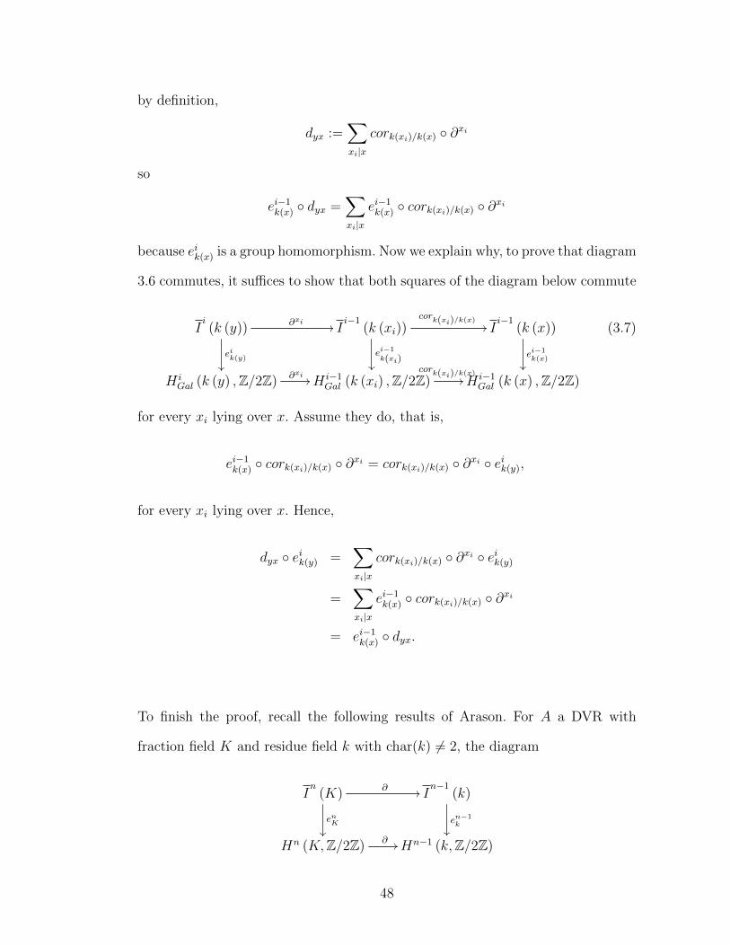
by definition,

dyx :=∑xi|x

cork(xi)/k(x) ◦ ∂xi

so

ei−1k(x) ◦ dyx =

∑xi|x

ei−1k(x) ◦ cork(xi)/k(x) ◦ ∂xi

because eik(x) is a group homomorphism. Now we explain why, to prove that diagram

3.6 commutes, it suffices to show that both squares of the diagram below commute

Ii(k (y)) ∂xi //

eik(y)

��

Ii−1

(k (xi))cork(xi)/k(x)

//

ei−1

k(xi)��

Ii−1

(k (x))

ei−1k(x)��

H iGal (k (y) ,Z/2Z) ∂xi // H i−1

Gal (k (xi) ,Z/2Z)cork(xi)/k(x)

// H i−1Gal (k (x) ,Z/2Z)

(3.7)

for every xi lying over x. Assume they do, that is,

ei−1k(x) ◦ cork(xi)/k(x) ◦ ∂xi = cork(xi)/k(x) ◦ ∂xi ◦ eik(y),

for every xi lying over x. Hence,

dyx ◦ eik(y) =∑xi|x

cork(xi)/k(x) ◦ ∂xi ◦ eik(y)

=∑xi|x

ei−1k(x) ◦ cork(xi)/k(x) ◦ ∂xi

= ei−1k(x) ◦ dyx.

To finish the proof, recall the following results of Arason. For A a DVR with

fraction field K and residue field k with char(k) 6= 2, the diagram

In

(K) ∂ //

enK��

In−1

(k)

en−1k��

Hn (K,Z/2Z) ∂ // Hn−1 (k,Z/2Z)

48

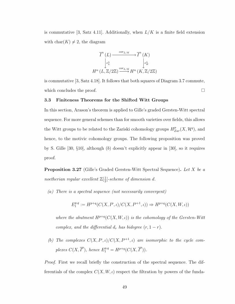
is commutative [3, Satz 4.11]. Additionally, when L/K is a finite field extension

with char(K) 6= 2, the diagram

In

(L)corL/K

//

enL��

In

(K)

enK��

Hn (L,Z/2Z)corL/K

// Hn (K,Z/2Z)

is commutative [3, Satz 4.18]. It follows that both squares of Diagram 3.7 commute,

which concludes the proof.

3.3 Finiteness Theorems for the Shifted Witt Groups

In this section, Arason’s theorem is applied to Gille’s graded Gersten-Witt spectral

sequence. For more general schemes than for smooth varieties over fields, this allows

the Witt groups to be related to the Zariski cohomology groups HpZar(X,Hq), and

hence, to the motivic cohomology groups. The following proposition was proved

by S. Gille [30, §10], although (b) doesn’t explicitly appear in [30], so it requires

proof.

Proposition 3.27 (Gille’s Graded Gersten-Witt Spectral Sequence). Let X be a

noetherian regular excellent Z[12]-scheme of dimension d.

(a) There is a spectral sequence (not necessarily convergent)

Ep,q1 := Hp+q(C(X, Ip, ι)/C(X, Ip+1, ι))⇒ Hp+q(C(X,W, ι))

where the abutment Hp+q(C(X,W, ι)) is the cohomology of the Gersten-Witt

complex, and the differential dr has bidegree (r, 1− r).

(b) The complexes C(X, Ip, ι)/C(X, Ip+1, ι) are isomorphic to the cycle com-

plexes C(X, Ip), hence Ep,q

1 = Hp+q(C(X, Ip)).

Proof. First we recall briefly the construction of the spectral sequence. The dif-

ferentials of the complex C(X,W, ι) respect the filtration by powers of the funda-

49

mental ideal [30, Theorem 6.6], hence we obtain a filtered complex

C(X, In, ι) :=⊕x∈X0

In (k (x))d→⊕x∈X1

In−1 (k (x))d→ . . . . . .

d→⊕x∈Xd

In−d (k (x)) ,

(3.8)

where we set Im (k (x)) = W (k (x)) when m ≤ 0. The exact sequence of complexes

0→ C(X, In+1, ι)→ C(X, In, ι)→ C(X, In, ι)/C(X, In+1, ι)→ 0

determines a long exact sequence in cohomology

→ Hp+q(C(X, In+1, ι))→ Hp+q(C(X, In, ι))→ Hp+q(C(X, Ip, ι)/C(X, Ip+1, ι))→

and setting Ep,q1 := Hp+q(C(X, Ip, ι)/C(X, Ip+1, ι)), we obtain an exact couple

which gives the spectral sequence of the proposition.

It remains to prove (b), that the quotient complexes obtained from C(X,W, ι)

agree with the cycle complexes (note that the quotient complexes do not depend on

the choices of isomorphisms ι [30, Definition 7.4 and Lemma 7.5]). For a smooth

variety over a field, the cycle complexes are exactly Rost’s cycle complexes for

the cycle module I∗, so in this situation, the assertion of (b) is exactly [30, §10.7].

Nevertheless, in the general case the proof is identical. First, recall that for integral

excellent rings, the integral closure is finite in the fraction field. The components

dyx : W (k (y)) //W (k (x))

of the differentials of the complex C(X,W, ι) may be described as follows: If y /∈

{x}, then dyx = 0. If x ∈ {y}, then

dyx :=∑xi|x

cork(xi)/k(x) ◦ ∂xi ,

where ∂xi denotes the residue map of Definition 3.23 and cork(xi)/k(x) the corestric-

tion of Definition 3.24 [30, conjugate Proposition 6.10 (taking L = K and B to

50

be the integral closure of A), and Proposition 6.5]. From this description of the

differential, together with Lemma 3.10, it follows that the n-th quotient complexes

C(X, In, ι)/C(X, In+1, ι) of the filtered complex C(X,W, ι) agree with the cycle

complex C(X, In) of Definition 3.25.

Applying Arason’s theorem (Theorem 3.26), we obtain the following corollary.

Corollary 3.28. Maintain the hypotheses of Proposition 3.27. The spectral se-

quence of Proposition 3.27 (not necessarily convergent) takes the form

Ep,q1 := Hp+q(C(X,Hp))⇒ Hp+q(C(X,W, ι)),

where Hp+q(C(X,Hp)) is the Kato cohomology of the p-th Kato complex.

Corollary 3.29. Let X be a pure separated scheme that is smooth over Z[12], and

suppose that no residue field of X is formally real. In this case, the spectral sequence

of Proposition 3.27 is convergent and takes the form

Ep,q1 := Hp+q

Zar (X,Hq)⇒ Hp+q(C(X,W, ι)),

where Hq denotes the Zariski sheaf associated to the presheaf U 7→ Hqet(U,Z/2Z).

Proof. Applying Corollary 3.13, we have that Hp+q(C(X,Hp)) = Hp+qZar (X,Hq).

Together with the previous Corollary 3.28, this yields the description of the E1-

terms. To prove convergence, note that as no residue field of X is formally real,

the cohomological dimension of X is 2dim(X) + 1 [1, Expose 5, §6, Theorem 6.2].

Hence, the groups Hp+qZar (X,Hq) vanish for p > 2dim(X) + 1, from which it follows

that the first page of the spectral sequence is bounded, and therefore the spectral

sequence strongly converges.

Proposition 3.30. Let X be a separated scheme that is pure and smooth over a

scheme S. Consider the following situations:

51

(a) dim(X) ≤ 1, no residue field of X is formally real, and S = Spec(Z[12]);

(b) dim(X) ≤ 2, X is quasi-projective, and S = Spec(Fp) (p > 2).

In either situation, the Witt groups W n(X) of X are finite.

Proof. In cases (a) and (b), the Kato cohomology is finite by Lemma 3.17 (a) and

(b), respectively. Hence, applying the convergent spectral sequence of Corollary

3.29, we obtain finiteness of the Gersten-Witt complex C(X,W, ι). To finish the

proof, use the convergent coniveau spectral sequence (Eq. (2.4)).

Next we note the following consequence of Mayer-Vietoris.

Lemma 3.31. Let S denote the category of noetherian regular separated Z[12]-

schemes.

(a) If, for any X in S, W n(X) is finite for all n in Z, then, for any X in S and

any line bundle L on X, W n(X,L) is finite for all n in Z.

(b) If, for every connected X in S, W n(X) is finite for all n in Z, then, for every

X in S, W n(X) is finite for all n in Z.

(c) If, for every affine X in S, W n(X) is finite for all n in Z, then, for every X

in S, W n(X) is finite for all n in Z.

Furthermore, the same statements are true with the Grothendieck-Witt groups in

place of Witt groups.

Proof. For noetherian regular separated schemes with 2 invertible, Mayer-Vietoris

holds for the Witt groups [8, Theorem 2.5], and for the Grothendieck-Witt groups

[61, Theorem 1.1]. For (a), recall that as line bundles are locally free, an open

cover of X on which L is trivial may be chosen. The lemma then follows by using

Mayer-Vietoris and inducting on the number of open sets in the cover.

52

Next recall that the connected components of any locally noetherian X are open

in X, and their intersection is empty. To prove (b), use Mayer-Vietoris, and proceed

by induction on the number of connected components of X.

Recall that for any separated scheme, the intersection of any two affine sub-

schemes is affine. To prove (c), use Mayer-Vietoris, and induct on the number of

affine open sets necessary to cover X.

The following well known lemma will be used together with the previous one to

reduce to X integral.

Lemma 3.32. If X is a noetherian regular connected scheme, then X is integral.

Proof. Let X be a noetherian regular connected scheme. As X is noetherian, it

has only a finite number of irreducible components and every local ring OX,x of

X is also noetherian [48, Chapter 2, Proposition 3.46(a)]. Since X has only a

finite number of irreducible components, it is integral if and only if it is connected

and integral at every point (i.e.OX,x is an integral domain for every x ∈ X) [48,

Chapter 2, Exercise 4.4]. To finish the proof, recall that every regular noetherian

local ring is a domain [48, Chapter 4, Proposition 2.11].

Theorem 3.33 (Absolute finiteness). Let X be a smooth variety over Fp (p > 2),

with dim(X) ≤ 2, and let L be a line bundle on X. In this situation, the Witt

groups W n(X,L) are finite for all n ∈ Z.

Proof. We may assume that X is connected using Lemma 3.31 (b), hence, in-

tegral, using Lemma 3.32. Using 3.31 (c), we may assume X is affine, hence

X → Fp is quasi-projective (any finite-type morphism between affine schemes

is quasi-projective). Proposition 3.30 (b), and Lemma 3.31 (a) finish the proof.

53

Theorem 3.34. Let X be a separated scheme that is smooth over Z[12], with no

residue field of X formally real. Assume the Beilinson-Lichtenbaum conjecture (see

Remark 3.19. Note that this is known for varieties over fields). If the motivic

cohomology groups Hmmot(X,Z/2Z(n)) are finite for all m,n ∈ Z, then the Witt

groups W n(X) are finite for all n ∈ Z.

Proof. We may assume that X is connected using Lemma 3.31 (b), hence, integral,

using Lemma 3.32. Using that the Beilinson-Lichtenbaum conjecture holds and

that the motivic cohomology groups Hmmot(X,Z/2Z(n)) are all finite, we apply

Lemma 3.20 to obtain that the Kato cohomology groups HmZar(X,Hn) are all finite.

Since the spectral sequence of Corollary 3.29 is convergent, the cohomology groups

of the Gersten-Witt complex C(X,W, ι) are finite. To finish the proof, use the

coniveau spectral sequence converging to the Witt groups of X (Eq. (2.4)).

For ease of reference we include the following corollary.

Corollary 3.35. Let X be a smooth variety over a finite field Fp (p > 2), and

let L be a line bundle on X. If the mod 2 motivic cohomology groups of X,

Hmmot(X,Z/2Z(n)), are finite for all m,n ∈ Z, then the Witt groups W n(X,L)

are finite for all n ∈ Z.

Finally, we note some partial converses to Theorem 3.34.

Theorem 3.36 (Relative finiteness). Let X be a regular separated scheme that

is of finite type over a base scheme S. Consider the following situations (for (a),

assume Beilinson-Lichtenbaum):

(a) dim(X) ≤ 2, no residue field of X is formally real, and S = Spec(Z[12]);

(b) dim(X) ≤ 3, X is connected and proper over S, and S = Spec(Fp) (p ≥ 2);

54

(c) dim(X) ≤ 4, X is connected and proper over S, and S = Spec(Fp) (p ≥ 2).

In situations (a) and (b):

(i) The Witt groups W 1(X) and W 3(X) are finite;

(ii) Finiteness of W 0(X) is equivalent to finiteness of W 2(X);

(iii) W 0(X) is finite if and only if the motivic cohomology groups Hpmot(X,Z/2Z(q))

are finite for all p, q ∈ Z.

In situation (c):

(i) The groups W 0(X) and CH3(X)/2CH3(X) are both finite if and only if the

motivic cohomology groups Hpmot(X,Z/2Z(q)) are finite for all p, q ∈ Z.

Proof. In all situations, finiteness of the Witt groups follows from finiteness of

motivic cohomology by Theorem 3.34, so we will only prove the other direction.

Assume that we are in situation (a). First we prove (i). To prove that W 1(X)

is finite, we will prove that the group H1(C(X,W, ι)) is finite, and then use the

coniveau spectral sequence (Eq. (2.4)). To prove that H1(C(X,W, ι)) is finite,

considering the spectral sequence of Corollary 3.29, it suffices to prove that the

groups on the on the p+ q = 1 diagonal of the first page of the spectral sequence,

H1Zar(X,Hp) for p ≥ 0, are finite. This was shown in Lemma 3.21 (a) (i). The proof

of finiteness of W 3(X) is identical.

Now we prove (ii). Assume that W 0(X) is finite. Considering the shape of the

coniveau spectral sequence (Eq. (2.4)), this implies H0(C(X,W, ι)) is finite. Con-

sidering the spectral sequence of Corollary 3.29, if we prove that all the groups

H2Zar(X,Hp) are finite, this will prove that H2(C(X,W, ι)) is finite, hence prove

that W 2(X) is finite. To accomplish this, using Lemma 3.21 (a) (i), it suffices

55

to prove that the groups H0Zar(X,H3), H0

Zar(X,H4), and H0Zar(X,H5) are finite.

Note that once we prove this, it will also finish the proof of (iii). Consider the

spectral sequence of Corollary 3.29. Since H0Zar(X,H5) has no non-zero differen-

tials entering or leaving it, it is stable, hence finite by finiteness of W 0(X). There

is one possibly non-zero differential leaving the group H0Zar(X,H4). It is the dif-

ferential d4,−41 : E4,−4

1 = H0Zar(X,H4) → E5,−4

1 = H1Zar(X,H5). Since the kernel of

d0,41 is stable, and is on the 0-th diagonal, it is finite by finiteness of W 0(X). So

finiteness of H0Zar(X,H4) follows from finiteness of H1

Zar(X,H5) (Lemma 3.21 (a)

(i)). Next, we will prove that H0Zar(X,H3) is finite. First, consider the differential

d3,−31 : E3,−3

1 = H0Zar(X,H3) → E4,−3

1 = H1Zar(X,H4). Since H1

Zar(X,H4) is finite,

H0Zar(X,H3) is finite if and only if the kernel of d3,−3

1 is finite. The kernel of d3,−31

equals E3,−32 . Consider the differential d3,−3

2 : E3,−32 → E5,−4

2 . Since H1Zar(X,H5) is

finite, its quotient E5,−42 is also finite. As the kernel of d3,−3

2 is on the 0-th diagonal

of the stable page, and W 0(X) is finite, we obtain finiteness of E3,−32 . Thus, prov-

ing that W 2(X) is finite. The proof that finiteness of W 2(X) implies finiteness of

W 0(X) is identical.

Assume that we are in situation (b). First we prove prove (i), finiteness ofW 1(X).

As in situation (a), it suffices to prove that the groups H1Zar(X,Hp) are finite, for

p ≥ 0. This was shown in Lemma 3.21 (b) (i). Similarly, we have that W 3(X) is

finite. Next, to prove (ii), assume W 0(X) is finite. Consider the spectral sequence

of Corollary 3.29. As E3,−31 = H0

Zar(X,H3) is on the 0-th diagonal of the stable

page, it is finite. So using Lemma 3.21 (b) (i) and (ii), this proves (iii), and we

have that all the groups H2Zar(X,Hp), for p ≥ 0, are finite, which proves finiteness

of W 2(X). The other direction is identical.

Finally, assume we are in situation (c). Consider the spectral sequence of Corol-

lary 3.29. By hypothesis W 0(X) is finite, so the stable term E4,−41 = H0

Zar(X,H4)

56

is finite. Additionally, by hypothesis CH3(X)/2CH3(X) = H3Zar(X,H3) is finite,

hence H1Zar(X,H4) is finite (Lemma 3.21 (c) (i)). Now consider the differential

d3,−31 : H0

Zar(X,H3)→ H1Zar(X,H4). As the kernel of d3,−3

1 is on the 0-th diagonal

of the stable page, it is finite by finiteness of W 1(X). Therefore, H0Zar(X,H3) is

finite, which is enough to finish the proof using Lemma 3.21 (c) (i).

57

The Gersten Conjecture

Let Λ be a DVR with infinite residue field. The purpose of this chapter is to prove

the Gersten conjecture for the Witt groups in the case of a local ring A that is

regular over Λ (Theorem 4.28). We first prove exactness of the augmented Gersten

complex in the case of A[π−1] (Theorem 4.19), where π is a uniformizing parameter

for Λ, A is essentially smooth over Λ, and A[π−1] is the localization at the element

π. For Witt groups, it follows from this result that the Gersten conjecture is also

true for A. As mentioned in the introduction, we use an adaptation of an argument

of S. Bloch which he used to prove exactness of the augmented Gersten complex

for K-theory in the case of A[π−1]. Also crucial is the work [31] of S. Gille and

J. Hornbostel. They developed an argument which replaces the usual concluding

argument of Quillen in the proof of the geometric case of the Gersten conjecture.

Finally, we adapt an argument of I. Panin to get from the essentially smooth case to

the regular over Λ case. In the following section we recall the definition and essential

properties that we need of Gille’s transfer map for the coherent Witt groups as

well as S. Gille’s revised zero-theorem. The remaining sections are devoted to the

proof.

4.1 The Transfer Map

We recall some results from from S. Gille’s paper [28].

Definition 4.1. Let π : R → S be a finite morphism of rings, in other words, a

morphism of rings such that S is finitely generated as an R-module. Given any

complex M• of S-modules, by restriction of scalars we obtain a complex π∗M•

of R-modules (i.e. , by considering each S-module Mi as an R-module via the

composition Rπ→ S → Mi). As restriction of scalars is functorial, we obtain a

58

functor

Dbcoh(M(S))→ Db

coh(M(R)) (4.1)

where Dbcoh(M(S)) is the full triangulated subcategory consisting of complexes

with coherent homology within the bounded derived category Db(M(S)) of S-

modules. When S is equipped with a dualizing complex I•, the finite map π de-

termines a dualizing complex on R which is denoted by π\(I•) [28, Theorem 4.1].

Furthermore [28, Definition 4.2 and preceeding material], there exists an isomor-

phism of dualities η : π∗χπ\(I) w→ χIπ∗ which makes the restriction of scalars functor

4.1 a morphism of triangulated categories with duality

(π∗, η) : (Dbcoh(M(S)), χπ

\(I), 1, $π\(I))→ (Dbcoh(M(R)), χI , 1, $I) (4.2)

and the morphism 4.2 induces on Witt groups a morphism

TrS/R : W i(S, π\(I•))→ W i(R, I•)

called the transfer morphism for the finite morphism π : R→ S.

Definition 4.2. Let R be a Gorenstein ring of finite Krull dimension, and t ∈

R a regular element, i.e. a non-zero divisor in R. Let j : R → I• be a finite

injective resolution of the R-module R. Let π : R → R/t be the quotient map.

The restriction of scalars functor respects the filtration by codimension of support,

that is,

π∗(Dj(R/tR)) ⊂ Dj+1(R)

and so, by restricting the morphism of triangulated categories with duality 4.2 to

Dj(R/tR), we have a morphism

(π∗, η) : Dj(R/tR)→ Dj+1(R)

59

and a morphism [26, Theorem 4.2] of triangulated Witt groups

Tr(R/tR)/R : W i(Dj(R/tR))→ W i+1(Dj+1(R)) (4.3)

called the transfer morphism. The composition of duality preserving functors

Dj(R/tR)(π∗,η)→ Dj+1(R)→ Dj(R),

where Dj+1(R) → Dj(R) is the inclusion, will be denoted by (π∗, ξ). The duality

preserving functor (π∗, ξ) induces a morphism [26, Theorem 4.2] of triangulated

Witt groups

Tr(R/tR)/R : W i(Dj(R/tR))→ W i+1(Dj(R)) (4.4)

which will also be called the transfer morphism. Since π∗M• ∈ Dj+1R/tR(R), where

DbR/tR(M(R)) denotes those complexes in Db

coh(M(R)) having homology vanishing

outside SpecR/tR and DjR/tR(R) those complexes in Db

R/tR(M(R)) with codimen-

sion of support less than or equal to j, the transfer morphism 4.3 factors in the

commutative diagram below

W i(Dj(R/tR)) Tr //

α∗��

W i+1(Dj+1(R))

W i+1(Dj+1R/tR(R))

55(4.5)

where α∗ is the devissage isomorphism [29, 3.1 and Theorem 3.2].

Lemma 4.3. Let R be a regular ring and t ∈ R a non-zero divisor. Then, if

y ∈ W i+1(Dj+1(R)) is such that the restriction of y to the open subset SpecRt ⊂

SpecR is zero, then there exists z ∈ W i(Dj(R/tR)) such that y = Tr(R/tR)/R(z).

Proof. Let y ∈ W i+1(Dj+1(R)) is such that the restriction of y to the open subset

SpecRt ⊂ SpecR is zero. The short exact sequence of triangulated categories with

duality [26, Section 2.6]

DbR/tR(M(R))→ Db

coh(M(R))→ Dbcoh(M(Rt)) (4.6)

60

determines, using the localization result for triangulated Witt groups (Proposition

2.7), the long exact sequence

. . .→ W i+1(DbR/tR(M(R)))→ W i+1(Db(M(R)))→ W i+1(Db(M(Rt)))→ . . .

Since the transfer morphism 4.3 factors through the devissage isomorphism (See

Definition 4.2) and y vanishes inW i+1(Db(M(Rt))), there exists z ∈ W i(Db(M(R/tR)))

such that y = Tr(R/tR)/R(z). However, then z ∈ W i(Dj(R/tR)) follows using the

definition of the transfer map and the fact that y ∈ W i+1(Dj+1(R)), finishing the

proof of the lemma.

Lemma 4.4. [28, Section 4 (i)] Maintain the hypotheses of Lemma 4.3. Then

the transfer for the Witt groups commutes with localization, in particular, for any

element f ∈ R, the diagram below commutes.

W i(Dp(R/tR)) Tr //

loc��

W i+1(Dp(R))

loc��

W i(Dp(Rf/tRf ))Tr //W i+1(Dp(Rf ))

Lemma 4.5. [28, Section 4 (ii)] Let R, S, T be Gorenstein rings, and let q : R→ S,

r : S → T , and s : R → T be finite morphisms such that s = r ◦ q. Then,

TrT/R = TrS/R · TrT/S.

Next we recall S. Gille’s new zero-theorem.

Proposition 4.6. [25, 24, Theorem 5.4 and Theorem 1.4, respectively] Let S,R,R′

be Gorenstein rings, and let ι : S → J•, γ : R → I• be injective resolutions of S

and R, respectively. Consider the commutative diagram

R

s��

R′

Sωoo

ψ__

61

where ω, ψ are flat morphisms, s is surjective and ker s = tR for some non-zero

divisor t ∈ R. If x is an i-symmetric space in Dj(S) with respect to the shifted

duality T−1χJ , then (s∗, ξ∗)∗(ω∗(x)) is a neutral i-symmetric space in Dj(R) with

respect to the duality χI .

For ease of reference we write down the corollary below. In view of the defi-

nition of the triangulated Witt groups, it immediately follows from the previous

proposition.

Corollary 4.7. Maintain the hypotheses of Proposition 4.6. Note that R′ ' R/tR,

and (s∗, ξ∗)∗(ω∗(x)) = Tr(R/tR)/R(ω∗(x)). Then, the morphism of Witt groups

W i−1(Dj(S))ω∗→ W i−1(Dj(R/tR))

Tr(R/tR)/R→ W i(Dj(R))

is zero.

4.2 Proof of the Gersten Conjecture: Essentially Smooth Case

First we recall some terminology, then we prove a series of lemmas leading to the

statement and proof of Theorem 4.19.

4.8. Recall that, given any local ring Λ, we say that a local Λ-algebra A is es-

sentially smooth over Λ if there exists a smooth Λ-algebra R and a prime ideal

n of R such that A is Λ-isomorphic to Rn and the composition homomorphism

Λ→ R→ Rn is local.

4.9. Let Λ be a DVR, π a uniformizing parameter for Λ. The generic point η is

open in Spec Λ as it is the complement of the unique closed point. For any Λ-

scheme X we will denote the fiber over the closed point of Λ by X0 (we will also

say the closed fiber) and the fiber over the generic point by Xη (we will say the

generic fiber). Recall that when X = SpecA is affine, then X0 = SpecA/π, and

62

the generic fiber of SpecA is then equal to SpecA⊗Λ FracΛ. Moreover, A⊗Λ FracΛ

is also equal to the localization Aπ = A[π−1] of A at the element π ∈ A.

Proposition 4.10. [38, Proposition 2.8.5] Let Y be a scheme that is locally noethe-

rian, irreducible, regular and of dimension 1, η the generic point, f : X → Y a

morphism, Xη = f−1(η) the fiber over the generic point, i : Xη → X the canonical

morphism, and Z a closed subscheme of Xη. Then the schematic closure Z (see

[34, Remark 10.31]) of the inclusion Z in X is the unique closed subscheme of X

which is flat as a Y -scheme and has i−1(Z) = Z, that is, the generic fiber Zη of Z

is Z.

Corollary 4.11. Maintain the hypotheses of Proposition 4.10. Additionally, as-

sume that Y = Λ is a DVR. The Λ-scheme X is flat over Λ if and only if X

equals the schematic closure Xη in X of the generic fiber Xη. If X is flat over

Λ, then every irreducible component of X dominates Λ (i.e. the image is dense,

or equivalently, the generic point of the irreducible component maps to the generic

point of Y ). If X is reduced, X is flat over Λ if and only if every every irreducible

component dominates Λ.

Proof. The first assertion follows immediately from Proposition 4.10. To prove the

second assertion, we begin by applying Proposition 4.10 to obtain that if X is flat

over Λ, then X equals the schematic closure Xη. To prove that the irreducible

components dominate we will prove that every generic point of X is in Xη. As the

underlying topological space of Xη is the topological closure of Xη, which is equal

as a set to the union⋃x∈Xη{x}, it follows that every generic point ξi of X is in the

closure {x} of a point x ∈ Xη. That is, every generic point ξi is the specialization

of a point x ∈ Xη. Since generic points are by definition the unique points which

specialize only to themselves, in other words, ξi ∈ {x} implies x = ξi, we obtain

63

that every generic point is in the generic fiber Xη. To prove the final assertion,

suppose that X is reduced and every irreducible component dominates Λ. Then,

as every generic point ξi is in Xη, the schematic closure of Xη has underlying

topological space X. A closed subscheme of a reduced scheme X that has the same

underlying topological space is necessarily equal as a scheme to X. Therefore X

equals the schematic closure of Xη and so X is flat.

Lemma 4.12. Let Λ be a DVR, π a uniformizing parameter for Λ, R a smooth

Λ-algebra, and p ∈ SpecR a prime ideal in R such that the composition Λ→ R→

Rp is a local morphism. Then, the Rp[π−1] equals the filtered colimit of the rings

Rf [π−1],

colimf /∈pRf [π−1]→ Rp[π

−1] (4.7)

where the colimit is taken over the set of elements f ∈ R such that f /∈ p.

Proof. For each f /∈ p we have the localization map Rf → Rp. A partial ordering

on R− p is given by f ≥ f′ ⇔ f = f

′f′′

for some f′/∈ p, in which case Rf ′ → Rf

is given by r/(f′)e 7→ r(f

′′)e/f e. So the colimit over the f /∈ p is filtered, and using

the universal property of the localization Rp it follows that the canonical map from

the filtered colimit

colimf /∈pRf → Rp (4.8)

is an isomorphism. As each map Rf ′ → Rf , and Rf → Rp, is a morphism of Λ-

algebras, they induce maps on the localizations Rf ′ [π−1] → Rf [π

−1], Rf [π−1] →

Rp[π−1]. Using the universal property of the localization Rp[π

−1] of Rp with respect

to the element π, it follows that the canonical map 4.7 is an isomorphism.

Lemma 4.13. Let Λ be a mixed (0, p)-characteristic (p 6= 2) DVR (see Appendix

5.11), π a uniformizing parameter for Λ, and A a local ring essentially smooth

64

over Λ. Let i, j ≥ 0 ∈ Z be integers, and let 0 6= x ∈ W i(Dj+1A[π−1]). Then, we

have the following:

(i) there exists a smooth integral Λ-algebra R with smooth integral closed fiber

R/π such that A ' Rp for some p ∈ Spec (R);

(ii) there exists an element in the Witt group y ∈ W i(Dj+1R[π−1]) such that y

maps to x via the morphism W i(Dj+1R[π−1])→ W i(Dj+1A[π−1]) induced by

the localization map R[π−1]→ A[π−1];

(iii) if A does not contain a field, then p lies in the closed fiber of SpecR;

(iv) there exists a non-zero-divisor t ∈ R such that SpecR/t is reduced and is flat

over Λ, and p lies in every irreducible component of SpecR/t;

(v) there exists an element in the Witt group z ∈ W i−1(Dj(R[π−1]/t)) such that

z maps to y under the transfer map Tr(R[π−1]/t)/R[π−1] : W i−1(DjR[π−1]/t)→

W i(Dj+1R[π−1]) for the finite morphism R[π−1]→ R[π−1]/t.

Proof. First recall that as A is essentially smooth over Λ, there exists a smooth

Λ-algebra R′

and a prime ideal p of R′

such that A is Λ-isomorphic to R′p and the

composition homomorphism A→ R′ → R

′p is local (Definition 4.8). Furthermore,

as x ∈ W i(Dj+1A[π−1]) and since Witt groups commute with filtered colimits [27,

Theorem 1.6], by Lemma 4.12 we have that x ∈ W i(Dj+1R′g[π−1]) for some g ∈ R′

such that g /∈ p. To prove (i), we will find a smaller basic open neighborhood

R′

f of p such that R′

f satisfies the assertions of (i). As R′

is smooth over Λ, the

closed fiber R′/π is smooth over Λ/π, from which it follows that (R

′/π)q is a

regular local ring at every prime ideal q in R′/π, hence R

′/π is a domain at every

point. The connected components of SpecR and SpecR′/π are open (any locally

noetherian space is locally connected [36, Corollary 6.1.9], which implies that the

65

connected components are open), so we may find f /∈ p such that SpecR′

f and

SpecR′

f/πR′

f are neighborhoods of p in SpecR′and SpecR

′/π, respectively, which

are each contained in a connected component. Furthermore, we may additionally

choose f /∈ p such that SpecR′

f is contained in the open subscheme SpecR′g. Then,

both R′

f and R′

f/πR′

f are connected and each is a domain at every point, hence

they are each integral [36, Corollary 6.1.12], smooth, and R′p ' Rp, proving (i).

To prove (ii), we take for y ∈ W i(Dj+1(R′

f )[π−1]) the image of x under the map

induced by localization R′g[π−1] → R

′

f [π−1]. By functoriality of the Witt groups,

y maps to x ∈ W i(Dj+1A[π−1]). Taking for R the localization R′

f proves (i) and

(ii). However, we note that for every basic open neighborhood R′

h of p contained

in R′

f , the assertions made in (i) and (ii) about R′

f remain true for R′

h. We will

need to choose smaller open neighborhoods of p to prove (iv) and (v), so we will

not take R′

f to be the R that appears in the statement of the lemma. However,

until we say otherwise, let R := R′

f for the remainder of the proof.

Now, to prove (iii) assume that A does not contain a field. To prove that

p ∈ SpecR is in the closed fiber p ∈ SpecR/π (hence in the closed fiber of any

smaller neighborhood SpecRg) suppose for the purpose of obtaining a contradic-

tion that p lies in the generic fiber SpecR⊗Λ FracΛ. In other words, suppose that

the prime ideal in Λ that is obtained by taking the inverse image of p under the

structure morphism Λ → R is the zero ideal. Then, after localizing, we obtain

the local homomorphism FracΛ → Rp: this homomorphism is necessarily injec-

tive (otherwise 1 ∈ Rp would be zero and A would be trivial) contradicting the

assumption that A does not contain a field.

We begin proving (iv) and (v) by choosing a representativeM• ∈ Dbcoh(M(R[π−1]))

for the underlying space of the element y ∈ W i(Dj+1R[π−1]). By definition, M• is

a bounded chain complex of R[π−1]-modules with finitely generated homology Hi.

66

As each Hi is finitely generated, the support SuppHi(M•) is a closed subspace in

SpecR[π−1] [34, Corollary 7.31]. Therefore, the support SuppM• of M• is a closed

subspace in SpecR[π−1] as it is a finite union

SuppM• = Supp⋃i

Hi(M•),

of closed subspaces. It follows from Proposition 4.10 that the closed subscheme

SuppM• defined by taking the schematic closure (see Proposition 4.10) of SuppM•

in SpecR is flat over Λ and has generic fiber (SuppM•)η = SuppM•. To prove (iv),

we first prove that the open complement SpecR − SuppM• has non-trivial inter-

section with the closed fiber SpecR0 = SpecR/π, and from this we deduce (iv).

Suppose, for the purpose of obtaining a contradiction, that SpecR0 ⊂ SuppM•.

In particular, we have an inclusion of closed fibers SpecR0 ⊂ SuppM•0. Then,

dimR− 1 = dimR0 ≤ dim SuppM•0 ≤ dim SuppM• ≤ dimR (4.9)

where dimR0 = dimR − 1 since R0 = R/π with R regular and π a non-zero

divisor. We will now prove that the center and the rightmost inequalities of 4.9 are

strict inequalities, which in view of 4.9, will result in the contradiction dimR−1 ≤

dimR− 2. If dim SuppM• = dimR, then from the inequality

dim SuppM• ≤ dim SuppM• + codim (SuppM•, SpecR) ≤ dimR

we have that codim (SuppM•, SpecR) = 0, or equivalently, that SuppM• contains

an irreducible component of SpecR [37, Proposition 14.2.2 (iv)]. As SpecR is

irreducible, this implies that SuppM• = SpecR, and in particular, that they have

the same generic fibers. Hence, SuppM• = SuppM•η = SpecRη, however, this

equality is not possible since

codim (SuppM•, SpecR[π−1]) 6= 0

67

as M• ∈ Dj+1R[π−1], and j + 1 is not equal to 0. This proves that dim SuppM• <

dimR. If dim SuppM•0 = dim SuppM•, then by the same reasoning as above, it fol-

lows that SuppM•0 contains an irreducible component of SuppM•. Yet this is im-

possible: since SuppM• is flat over Λ, every irreducible component of SuppM• dom-

inates Λ (Corollary 4.11), hence the generic points of SuppM• are contained in the

generic fiber SuppM•, and thus cannot be contained in the closed fiber SuppM•0.

This concludes the proof of the claim that (SpecR− SuppM•) ∩ SpecR0 6= ∅.

Applying what we have just proved, let q ∈ (SpecR − SuppM•) ∩ SpecR0.

Choose a principal open neighborhood SpecRt of q which is contained in the open

complement SpecR−SuppM•. That is, SpecRt∩SuppM• = ∅, so SpecRt[π−1]∩

SuppM• = ∅. As q ∈ SpecRt ∩ SpecR0 = Spec (R/π)t, it follows that t ∈ R

is not nilpotent in R/π, in particular, it is non-zero in R/π. We will now prove

that R/t is flat over Λ. To do so, it suffices to prove that R/t is torsion free as a

Λ-module [48, Chapter 1, Corollary 2.5]. Since Λ is a DVR, if R/t has no π-torsion,

then R/t is torsion free over Λ. Assume that R/t has π-torsion for the purpose of

obtaining a contradiction. Then, there exists 0 6= a ∈ R/t such that πa = 0 ∈ R/t,

that is, πa = tb for some b ∈ R and a /∈ tR. Using the hypothesis that R/π is a

domain, it follows that t ∈ R/π is not a zero-divisor in R/π, hence πa = tb implies

b ∈ πR, that is, b = πc for some c ∈ R. Since R is a domain, from πa = tπc we

obtain by cancelation that a = tc, a contradiction. This proves that R/t is flat over

Λ. Then, all irreducible components of SpecR/t dominate (Lemma 4.14) so it it

follows that Spec (R/t)red is also flat over Λ (Corollary 4.11). As the localization

Rp is a unique factorization domain, we may take tp = ta11 · · · tann to be a factoriza-

tion of tp. Then Spec (Rp/tp)red = SpecRp/t1 · · · tn. We may choose a sufficiently

small open neighborhood SpecRf of p such that Spec (Rf/t)red = SpecRf/t1 · · · tn.

Then, set R := Rf and t := t1 · · · tn. Restricting y to R, with M• denoting the

68

complex representing y, we again have that Rt[π−1] ∩ SuppM• = ∅. Therefore,

y ∈ W i(Dj+1Rt[π−1]) is zero. From this, we have that if p ∈ SpecR is not in the

image of the closed subscheme SpecR/tR, then it must be in the image of the

complement p ∈ SpecRt, that is, t /∈ p. However, in this case it would follow that

the element x ∈ W i(Dj+1A[π−1]) is zero (using the fact that W i(Dj+1A[π−1]) is

a colimit of W i(Dj+1Rt[π−1]) over t /∈ p). This would contradict the hypothesis

that x 6= 0. So, p ∈ SpecR/t. Now we prove the assertions about the irreducible

components: the irreducible components of SpecR/t are closed and finite in num-

ber; the union of the irreducible components which do not contain p is closed and

does not contain p, so its complement is an open neighborhood U of p; choosing a

principal open neighborhood SpecRf/t contained in U we have that the irreducible

components of SpecRf/tRf all meet p. This completes the proof of (iv). To prove

(v), let y again denote the restriction of y to Rf . Then, y ∈ W i(Dj+1Rt[π−1]) is

zero, so the map of Witt groups W i(Dj+1R[π−1])→ W i(Dj+1(R[π−1])t) that is in-

duced by the open immersion SpecRt[π−1]→ SpecR[π−1] sends y to 0. Therefore,

there exists z ∈ W i(Dj(R[π−1]/tR[π−1])) such that y = Tr(R[π−1]/tR[π−1])/R[π−1](z)

(Lemma 4.3). This completes the proof of the lemma.

Lemma 4.14. Let Λ be a DVR, and let Y ⊂ Z be a quasi-compact morphism of

Λ-schemes, with Y a reduced scheme which is flat over Λ. If Y is the schematic

closure of Y in Z, then Y is flat over Λ.

Proof. As Y ⊂ Z is a quasi-compact morphism the schematic closure Y of Y

in Z exists and is reduced whenever Y is reduced [36, Proposition 9.5.9]. As Y is

reduced, to prove that Y is flat over Λ, it suffices to demonstrate that the irreducible

components of Y dominate Λ (Corollary 4.11). The irreducible components of Y

are the closures Yi in Z of the irreducible components Yi of Y . If Y is flat over Λ,

69

then the irreducible components Yi of Y dominate Λ (Corollary 4.11). Since the

inclusion Yi ↪→ Yi is also dominant, it follows that Yi → Λ is dominant, and hence

the irreducible components Yi dominate Λ.

Proposition 4.15. [34, Proposition 14.107] Let Y be a noetherian scheme, and

let f : X → Y be a morphism of finite type. Assume in addition that X and Y

are irreducible, that Y is universally catenary (e.g. a regular ring is universally

catenary), and that f is surjective. Then dimX = dimY + Xη, where η is the

generic point of Y .

Lemma 4.16. Let Λ be a mixed (0, p)-characteristic (p 6= 2) DVR (see Appendix

5.11), and R a smooth integral Λ-algebra, t ∈ R a non-zero divisor such that

SpecR/t is reduced and flat over Λ, and x ∈ SpecR/t. Suppose that dimR/π = d.

As R is of finite type over Λ, by definition R := Λ[X1, . . . , Xn]/〈f1, . . . , fr〉. The

surjection Λ[X1, . . . , Xn] → R induces a closed immersion SpecR ↪→ AnΛ. Embed

AnΛ ↪→ PnΛ as the complement of a hyperplane. Let Y,X denote the schemes ob-

tained taking the schematic closures of SpecR/t, SpecR in PnΛ, respectively (equiv-

alently, take their topological closures with the reduced, induced, subscheme struc-

ture). Then, Y is locally a principal divisor on X at x (i.e.Y is at x a regular

immersion of codimension 1), Y and X are flat over Λ, and dimX = d + 1,

dimX0 = dimXη = d.

Proof. Since SpecR/t is a principal divisor on SpecR, it follows that Y is locally

a principal divisor on X at x. Flatness of Y,X, follow from Lemma 4.14. Now

we prove the assertions about the dimensions. As π ∈ R is a non-zero divisor, it

follows that dimR = d + 1. Applying Proposition 4.15 to SpecR → Λ (which we

may use since x is in the closed fiber SpecR/π and SpecR dominates Λ, hence

SpecR surjects onto Λ) we have that dim SpecRη = d. Since SpecRη → Xη is

70

an open dense inclusion of FracΛ-varieties, it follows that dim SpecRη = dimXη.

Then, applying Proposition 4.15 to X, we have that dimX = d + 1. Since X

dominates, the closed fiber cannot contain an irreducible component, equivalently,

codim (X0, X) ≥ 1, and hence dimX0 < dimX. Therefore, from the inclusions

SpecR/π ⊂ X0 ⊂ X we have that d = dim SpecR/π ≤ dimX0 < dimX = d + 1,

hence dimX0 = d.

The next proposition is Bloch’s geometric Lemma and it is crucial for the proof

of Theorem 4.19.

Proposition 4.17. [14, SubLemma A.4] Let Λ be a mixed (0, p)-characteristic

(p 6= 2) DVR (see Appendix 5.11) with infinite residue field, and A a local ring

essentially smooth over Λ. Let X ↪→ PnΛ be a projective variety over Λ, x ∈ X0 an

element in the closed fiber of X such that OX,x w A, and assume that X is smooth

over Λ at x. Let d denote the dimension of X0. Let Yj↪→ X be locally at x a

principal divisor with Y flat over Λ, and let Wη ↪→ Yη be a closed subscheme of the

generic fiber Yη of Y such that dimWη < dimYη. Let W be the schematic closure of

Wη in X (the notation is reasonable since the generic fiber of W is exactly Wη by

Lemma 4.14) and assume that x /∈ W . Then, there exists a commutative diagram

U

π��

Yπ|Y //

j==

Pd−1Λ

(4.10)

where U is an open neighborhood of x in X, π is smooth at x over Pd−1Λ of relative

dimension 1, π|Y is a finite morphism, and π(x) /∈ π(W ).

Corollary 4.18. Maintain the hypotheses of Lemma 4.16. Then, there exists an

open affine subscheme SpecC ⊂ Y containing x, for some f ∈ R an open immer-

71

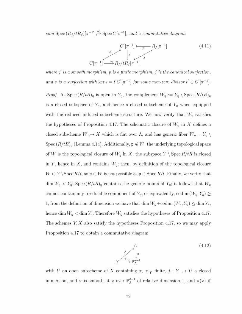
sion Spec (Rf/tRf )[π−1]

ω↪→ SpecC[π−1], and a commutative diagram

C′[π−1]

s

��

Rf [π−1]p

oo

jxx

C[π−1] ω //

ψ88

Rf/tRf [π−1]

(4.11)

where ψ is a smooth morphism, p is a finite morphism, j is the canonical surjection,

and s is a surjection with ker s = t′C′[π−1] for some non-zero divisor t

′ ∈ C ′ [π−1].

Proof. As Spec (R/tR)η is open in Yη, the complement Wη := Yη \ Spec (R/tR)η

is a closed subspace of Yη, and hence a closed subscheme of Yη when equipped

with the reduced induced subscheme structure. We now verify that Wη satisfies

the hypotheses of Proposition 4.17. The schematic closure of Wη in X defines a

closed subscheme W ↪→ X which is flat over Λ, and has generic fiber Wη = Yη \

Spec (R/tR)η (Lemma 4.14). Additionally, p /∈ W : the underlying topological space

of W is the topological closure of Wη in X; the subspace Y \ SpecR/tR is closed

in Y , hence in X, and contains Wη; then, by definition of the topological closure

W ⊂ Y \SpecR/t, so p ∈ W is not possible as p ∈ SpecR/t. Finally, we verify that

dimWη < Yη: Spec (R/tR)η contains the generic points of Yη; it follows that Wη

cannot contain any irreducible component of Yη, or equivalently, codim (Wη, Yη) ≥

1; from the definition of dimension we have that dimWη+codim (Wη, Yη) ≤ dimYη,

hence dimWη < dimYη. Therefore Wη satisfies the hypotheses of Proposition 4.17.

The schemes Y,X also satisfy the hypotheses Proposition 4.17, so we may apply

Proposition 4.17 to obtain a commutative diagram

U

π��

Yπ|Y //

j==

Pd−1Λ

(4.12)

with U an open subscheme of X containing x, π|Y finite, j : Y ↪→ U a closed

immersion, and π is smooth at x over Pd−1Λ of relative dimension 1, and π(x) /∈

72

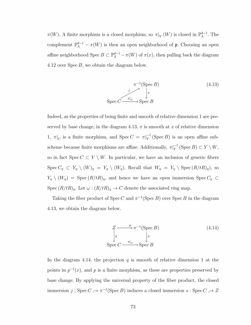
π(W ). A finite morphism is a closed morphism, so π|Y (W ) is closed in Pd−1Λ . The

complement Pd−1Λ − π(W ) is then an open neighborhood of p. Choosing an open

affine neighborhood SpecB ⊂ Pd−1Λ −π(W ) of π(x), then pulling back the diagram

4.12 over SpecB, we obtain the diagram below.

π−1(SpecB)

π

��

SpecCπ|C //

j77

SpecB

(4.13)

Indeed, as the properties of being finite and smooth of relative dimension 1 are pre-

served by base change, in the diagram 4.13, π is smooth at x of relative dimension

1, π|C is a finite morphism, and SpecC = π|−1Y (SpecB) is an open affine sub-

scheme because finite morphisms are affine. Additionally, π|−1Y (SpecB) ⊂ Y \W ,

so in fact SpecC ⊂ Y \W . In particular, we have an inclusion of generic fibers

SpecCη ⊂ Yη \ (W )η = Yη \ (Wη). Recall that Wη = Yη \ Spec (R/tR)η), so

Yη \ (Wη) = Spec (R/tR)η, and hence we have an open immersion SpecCη ⊂

Spec (R/tR)η. Let ω : (R/tR)η → C denote the associated ring map.

Taking the fiber product of SpecC and π−1(SpecB) over SpecB in the diagram

4.13, we obtain the diagram below.

Zp//

q

��

π−1(SpecB)

π

��

SpecCπ|C // SpecB

(4.14)

In the diagram 4.14, the projection q is smooth of relative dimension 1 at the

points in p−1(x), and p is a finite morphism, as these are properties preserved by

base change. By applying the universal property of the fiber product, the closed

immersion j : SpecC ↪→ π−1(SpecB) induces a closed immersion s : SpecC ↪→ Z

73

which is a section of q : Z → SpecC such that the diagram below commutes.

Zp// π−1(SpecB)

SpecC

j77

s

OO (4.15)

We have then [2, 4.15] that the sheaf of ideals in OZ defining the image of s is

principal, defined by a regular element (that is, a non-zero divisor) at the points

p−1(x), hence principal in a neighborhood U of p−1(x). Since p is a finite morphism,

it is a closed morphism, and then p(Z − U) is closed in π−1(SpecB) and does not

contain x. Choose an open neighborhood SpecRf (recall that SpecR is open in

X) of x such that: SpecRf is contained in π−1(SpecB) − p(Z − U); SpecRf is

smooth over SpecB. Then, as p is an affine morphism, p−1(SpecRf ) is affine and

will be denoted by SpecC′.

Now, we have by pulling back the smooth morphism π : SpecRf ↪→ π−1(SpecB)π→

SpecB along π|C : SpecC → SpecB the diagram

SpecC′ p

//

��

SpecRf

��

Zp//

q

��

π−1(SpecB)

π

��

SpecCπ|C // SpecB

with SpecC′↪→ Z

q→ SpecC a smooth morphism as it is a base change of a

smooth morphism. Denote this smooth morphism by ψ : SpecC′ → SpecC. Then,

pulling back the diagram 4.15 along the open immersion SpecRf → π−1(SpecB)

we obtain the commutative diagram below (using the definition of the fiber product

we identify j−1(SpecRf ) with SpecRf/tRf ).

74

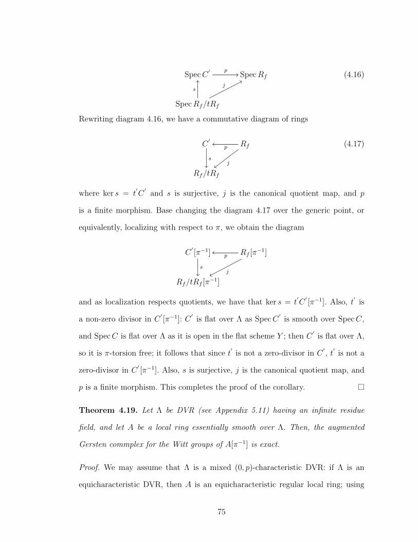
SpecC′ p

// SpecRf

SpecRf/tRf

j77

s

OO(4.16)

Rewriting diagram 4.16, we have a commutative diagram of rings

C′

s

��

Rfpoo

j{{

Rf/tRf

(4.17)

where ker s = t′C′

and s is surjective, j is the canonical quotient map, and p

is a finite morphism. Base changing the diagram 4.17 over the generic point, or

equivalently, localizing with respect to π, we obtain the diagram

C′[π−1]

s

��

Rf [π−1]p

oo

jxx

Rf/tRf [π−1]

and as localization respects quotients, we have that ker s = t′C′[π−1]. Also, t

′is

a non-zero divisor in C′[π−1]: C

′is flat over Λ as SpecC

′is smooth over SpecC,

and SpecC is flat over Λ as it is open in the flat scheme Y ; then C′

is flat over Λ,

so it is π-torsion free; it follows that since t′

is not a zero-divisor in C′, t′

is not a

zero-divisor in C′[π−1]. Also, s is surjective, j is the canonical quotient map, and

p is a finite morphism. This completes the proof of the corollary.

Theorem 4.19. Let Λ be DVR (see Appendix 5.11) having an infinite residue

field, and let A be a local ring essentially smooth over Λ. Then, the augmented

Gersten commplex for the Witt groups of A[π−1] is exact.

Proof. We may assume that Λ is a mixed (0, p)-characteristic DVR: if Λ is an

equicharacteristic DVR, then A is an equicharacteristic regular local ring; using

75

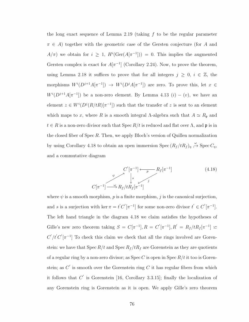
the long exact sequence of Lemma 2.19 (taking f to be the regular parameter

π ∈ A) together with the geometric case of the Gersten conjecture (for A and

A/π) we obtain for i ≥ 1, H i(Ger(A[π−1])) = 0. This implies the augmented

Gersten complex is exact for A[π−1] (Corollary 2.24). Now, to prove the theorem,

using Lemma 2.18 it suffices to prove that for all integers j ≥ 0, i ∈ Z, the

morphisms W i(Dj+1A[π−1]) → W i(DjA[π−1]) are zero. To prove this, let x ∈

W i(Dj+1A[π−1]) be a non-zero element. By Lemma 4.13 (i) − (v), we have an

element z ∈ W i(Dj(R/tR)[π−1]) such that the transfer of z is sent to an element

which maps to x, where R is a smooth integral Λ-algebra such that A ' Rp and

t ∈ R is a non-zero divisor such that SpecR/t is reduced and flat over Λ, and p is in

the closed fiber of SpecR. Then, we apply Bloch’s version of Quillen normalization

by using Corollary 4.18 to obtain an open immersion Spec (Rf/tRf )ηω↪→ SpecCη,

and a commutative diagram

C′[π−1]

s

��

Rf [π−1]p

oo

jxx

C[π−1] ω //

ψ88

Rf/tRf [π−1]

(4.18)

where ψ is a smooth morphism, p is a finite morphism, j is the canonical surjection,

and s is a surjection with kerπ = t′C′[π−1] for some non-zero divisor t

′ ∈ C ′ [π−1].

The left hand triangle in the diagram 4.18 we claim satisfies the hypotheses of

Gille’s new zero theorem taking S = C[π−1], R = C′[π−1], R

′= Rf/tRf [π

−1] w

C′/t′C′[π−1] To check this claim we check that all the rings involved are Goren-

stein: we have that SpecR/t and SpecRf/tRf are Gorenstein as they are quotients

of a regular ring by a non-zero divisor; as SpecC is open in SpecR/t it too is Goren-

stein; as C′

is smooth over the Gorenstein ring C it has regular fibers from which

it follows that C′

is Gorenstein [16, Corollary 3.3.15]; finally the localization of

any Gorenstein ring is Gorenstein as it is open. We apply Gille’s zero theorem

76

using Corollary 4.7. From this result we have that the morphism of Witt groups

W i−1(DjC[π−1])ω∗→ W i−1(DjC

′[π−1]/t

′C′[π−1])

Tr→ W i(DjC′[π−1]) is zero. Since

the transfer commutes with the composition of finite morphisms (Lemma 4.5),

from the commutative diagram appearing in the righthand triangle of diagram

4.18 we obtain that the composition

W i−1(DjC[π−1])ω∗→ W i−1(DjRf/tRf [π

−1])Tr→ W i(DjRf [π

−1])

is zero. As the transfer commutes with localization (Lemma 4.4), the diagram

below commutes

W i−1(DjR/tR[π−1])

tt

Tr //

��

W i(DjR[π−1])

��

W i−1(DjC[π−1]) ω∗ //W i−1(DjRf/tRf [π−1]) Tr //W i(DjRf [π

−1])

where the maps in the left hand triangle are induced from open immersions. This

finishes the proof since then the image of x in W i(DjA[π−1]) is zero as it is the

image of z and we just proved that z maps to zero in W i(DjRf [π−1]).

Corollary 4.20. Let Λ be a DVR having an infinite residue field, π a uniformizing

parameter for Λ, and A a local ring essentially smooth over Λ. Then, the Gersten

conjecture is true for the Witt groups of A.

Proof. If Λ is an equicharacteristic DVR, then it follows that A is equicharacteristic

regular local ring, in which case the Gersten conjecture is known (e.g. [31, Theorem

3.1]). So we may assume that Λ is a mixed (0, p)-characteristic (p 6= 2) DVR.

Then, using the long exact sequence of Lemma 2.19 (taking f to be the regular

parameter π ∈ A) together with Theorem 4.19 and the geometric case applied to

the equicharacteristic regular local ring A/π (e.g. [31, Theorem 3.1]) of the Gersten

conjecture for the Witt group we have that, for i ≥ 2, H i(Ger(A)) = 0. This implies

the Gersten conjecture for A (Corollary 2.24).

77

Corollary 4.21. Let Λ be a DVR having an infinite residue field, π a uniformizing

parameter for Λ, and A a local ring essentially smooth over Λ. Then, for p ≥ 1,

HpZar(A[π−1],W) = 0, that is, the Zariski cohomology of A[π−1] with coefficients in

the Witt sheaf (the Zariski sheaf on SpecA associated to the presheaf U 7→ W (U))

vanishes.

Proof. Using Theorem 4.19 we have that, for p ≥ 1, Hp(Ger(A[π−1])) = 0. Since

the Gersten conjecture is also true for every local ring of A[π−1] by the geo-

metric case of the Gersten conjecture, we then have that Hp(Ger(A[π−1])) =

HpZar(A[π−1],W) (Lemma 2.17), thus proving the corollary.

4.3 Proof of the Gersten Conjecture: Local Rings Regular over aDVR

4.22. Let k be a field and R a noetherian k-algebra, that is, R is a noetherian

ring together with a ring morphism k → R from the field k to R. For every field

extension k → k′

of k, we may consider the k′-algebra R⊗k k

′obtained by taking

the tensor product of R and k′over k; if, for every finite field extension k

′, R⊗kk

′is

a regular ring, then R is said to be geometrically regular over k. When, additionally,

R is local, then R is geometrically regular over k if and only if R is formally smooth

(with the mR-adic topology) over k [37, 22.5.8].

4.23. A morphism A′ → A of noetherian rings is regular if it is flat and for every

p ∈ SpecA, the fiber A⊗A′ k(p) is geometrically regular over k(p).

Lemma 4.24. Let Λ be a DVR, π a uniformizing parameter for Λ, and A a regular

local ring of mixed (0, p)-characteristic which is a Λ-algebra. If A is regular over

Λ, then π is a regular parameter for A, and additionally:

(i) the closed fiber A/π of A over Λ is a regular local ring of equicharacteristic

p;

78

(ii) the localizations (A[π−1])p of A[π−1] at prime ideals p ∈ SpecA[π−1] are

regular local rings of equicharacteristic 0.

Proof. Since A is regular over Λ, from the definition we have that the closed fiber

A/π is geometrically regular over Λ/π, hence is regular. As the quotient A/π is

regular of dimension dimA− 1, it follows that π is a regular parameter for A.

As A is a mixed (0, p)-characteristic regular local ring that is a Λ-algebra, Λ is

contained in A and is also of mixed (0, p)-characteristic (Lemma 5.12). In particular

the prime p is an element p ∈ mA of the maximal ideal mA in A. Hence, the closed

fiber A/π is a regular local ring of equicharacteristic p, proving (i).

To prove (ii), in view of the fact that for any prime p ∈ SpecA[π−1] the local-

izations commute (A[π−1])p = Ap, it follows that they are regular local rings, and

as they are Q-algebras via the composition Q ↪→ FracΛ → A[π−1] → (A[π−1])p,

they are regular local of equicharacteristic 0.

Next we recall Popescu’s theorem below, and apply it in Lemma 4.26.

Proposition 4.25. [57, Theorem 1.8] Let A′ → A be a homomorphism of noethe-

rian rings. The homomorphism A′ → A is a regular morphism if and only if A is

a filtered colimit of smooth A′-algebras.

In the following Lemma (i) is immediate and the proof of (ii) follows since in

this case the localization at an element commutes with the filtered colimit.

Lemma 4.26. [55, c.f. Lemma 3.2] Let Λ be a DVR, π a uniformizing parameter

for Λ, and A a local ring regular over Λ, that is, A is a filtered colimit of smooth

Λ-algebras Sα (Proposition 4.25). Let φα : Sα → A denote the canonical homomor-

phisms into the colimit. Denote by pα the prime ideal in Sα defined by the inverse

79

image of the maximal ideal φ−1α (mA). Let Spα denote the localization of Sα at the

prime ideal pα. Then:

(i) the ring A is a filtered colimit A ' lim−→Spα, where the Spα are regular local

rings which are essentially smooth over Λ;

(ii) the localization A[π−1] of A at the element π is a filtered colimit A[π−1] '

lim−→(Spα)[π−1], where (Spα)[π−1] is the localization of Spα at the element π.

Lemma 4.27. Let A be a regular local ring, and f ∈ A be a regular parameter on

A. Suppose that the following two conditions are satisfied:

i) the Gersten conjecture is true for the Witt groups of the quotient ring A/fA;

ii) for every prime p ∈ SpecAf , the Gersten conjecture is true for the Witt

groups of the localization (Af )p = Ap.

Under these conditions, if the Zariski cohomology groups HpZar(Af ,W) of Af with

coefficients in the Witt sheaf W vanish for p ≥ 2, then the Gersten conjecture is

true for the Witt groups of A.

Proof. Let A be a regular local ring, and let f ∈ A be a regular parameter on A.

The quotient ring A/fA is again a regular local ring, of Krull dimension equal to

dimA − 1. Suppose that i) holds, that is, the Gersten conjecture is true for the

Witt groups of A/fA. In particular, for p ≥ 1, the cohomology of the Gersten-Witt

complex for A/fA vanishes, Hp(Ger(A/fA)) = 0. Then, in view of the localization

long exact sequence 2.15 of Lemma 2.19, when p ≥ 2 the cohomology of the

Gersten-Witt complexHp(Ger(A)) of A injects into the cohomology of the Gersten-

Witt complex Hp(Ger(Af )) of Af . It follows that if Hp(Ger(Af )) = 0 for p ≥ 2,

then Hp(Ger(A)) = 0 for p ≥ 2, or equivalently, the Gersten conjecture is true for

80

the Witt groups of A. If we additionally suppose ii), that is, for every prime ideal

p ∈ SpecAf of Af , the Gersten conjecture is true for the Witt groups of (Af )p = Ap,

then we have by Lemma 2.17 that the Zariski cohomology groups HpZar(Af ,W) of

Af with coefficients in the Witt sheaf W are equal to the cohomology of the

Gersten-Witt complex Hp(Ger(Af )) of Af . From these observations, the lemma

immediately follows.

To conclude this chapter, we prove the Gersten conjecture for the Witt groups

of a local ring regular over a DVR having infinite residue field.

Theorem 4.28. Let Λ be a DVR having an infinite residue field. If A is a local

ring that is regular over Λ, then the Gersten conjecture is true for the Witt groups

of A.

Proof. Let A be a local ring that is regular over Λ, and let π denote a uniformiz-

ing parameter for Λ. As the Gersten conjecture is known when A is of equichar-

acteristic, we may assume that both Λ and A are of mixed (0, p)-characteristic

(Lemma 5.12). To prove the Gersten conjecture for the Witt groups of A, we

first demonstrate that it is sufficient to prove that the Zariski cohomology groups

HpZar(A[π−1],W) of A[π−1] with coefficients in the Witt sheafW vanish when p ≥ 2.

To prove this sufficiency, we will verify that π is a regular parameter satisfying the

conditions of Lemma 4.27. Applying Lemma 4.24, we have that π ∈ A is a reg-

ular parameter of A such that: i) the closed fiber A/π of Λ → A is a regular

local ring of equicharacteristic p; ii) the localizations (A[π−1])p of A[π−1] at prime

ideals p ∈ SpecA[π−1] are regular local rings of equicharacteristic 0. Using the

equicharacteristic case of the Gersten conjecture, we then have that the Gersten

conjecture is true for A/π and for the local rings (A[π−1])p. Hence π satisfies the

desired conditions.

81

To prove the vanishing of the Zariski cohomology groups HpZar(A[π−1],W), we

begin by writing A[π−1] as a filtered colimit of rings (Spα)[π−1] (Lemma 4.26),

where each (Spα)[π−1] is the localization at π of a local ring Spα which is essentially

smooth over Λ. Zariski cohomology commutes with filtered colimits (a theorem due

to Grothendieck, however see [55, Theorem 6.6] for an alternative proof), hence

this finishes the proof since the Zariski cohomology groups HpZar((Spα)[π−1],W)

vanish when p ≥ 2 (Corollary 4.21).

82

Applications

5.1 Finite Generation Theorems for Grothendieck-Witt Groups

In this section, we prove finite generation theorems for the Grothendieck-Witt

groups of arithmetic schemes. Let X be a separated noetherian scheme over Z[12],

and let L be a line bundle on X. Let ChbVect(X) denote the category of bounded

chain complexes of vector bundles on X. By shifting L, for each n ∈ Z, we obtain a

duality Hom(−, L[n]) on ChbVect(X). We work with Schlichting’s Grothendieck-

Witt spectrum GW n(X,L) [63] associated to the category ChbVect(X), equipped

with the duality Hom(−, L[n]) and with quasi-isomorphisms as weak equivalences.

Its m-th homotopy groups are denoted by GW nm(X,L), and are said to be the

Grothendieck-Witt groups of X with coefficients in L. These groups are 4-periodic

in n, GW nm(X,L) ' GW n+4

m (X,L). The negative Grothendieck-Witt groups, that

is, the negative homotopy groups of the Grothendieck-Witt spectrum, agree with

the Witt groups GW 0−m(X) ' Wm(X), for m > 0. For these facts, see [63].

Proposition 5.1. Let X be a separated noetherian regular Z[12]-scheme. For every

n ∈ Z, there is a long exact sequence of abelian groups

. . .→ GW nm(X)→ GW n−1

m−1(X)F→ Km−1(X)

H→ GW nm−1(X)→ . . .

which may be completed to end in

. . . GW n−10 (X)→ K0(X)

H→ GW n0 (X)→ W n(X)→ 0.

Proof. It is proved in [63] that the sequence of spectra

GW n−1(X)F→ K(X)

H→ GW n(X)

is a homotopy fibration, where K(X) is the algebraic K-theory spectrum whose

homotopy groups are the higher algebraic K-groups. Hence, it determines the

83

long exact sequence of the proposition, with one exception. To complete the long

exact sequence to the form stated in the proposition, we use the isomorphism

GW 0−m(X) ' Wm(X) (m > 0) [63], which gives GW 0

−1(X) ' W 1(X). Shifting

the duality on both sides (n − 1)-times, we obtain GW n−1−1 (X) ' W n(X). Since

there are no negative K-groups of X, the map GW n0 (X) → W n(X) is surjective

as asserted.

Karoubi induction is a well known means of proving the corollary below. We give

the corollary the name “Schlichting” induction because the argument is different

than the usual Karoubi induction argument (i.e. it uses the fibration above), and

it was suggested to the author by Schlichting.

Corollary 5.2 (“Schlichting” Induction). Maintain the hypothesis of the previous

proposition. Assume that the groups Km(X) are finitely generated for all m ∈ Z. If

the Witt groups W n(X) are finitely generated for all n ∈ Z, then the Grothendieck-

Witt groups GW nm(X) are finitely generated for all m,n ∈ Z.

Proof. We will prove the result by induction on m. The base case is m = −1,

finite generation of the Witt groups W n(X) ' GW n−1−1 , for all n ∈ Z. For the

induction step, suppose that GW n−1m−1(X) is finitely generated, for all n ∈ Z. Using

the fibration sequence of Proposition 5.1, and finite generation of the algebraic

K-theory groups Km(X), we obtain that GW nm(X) is also finitely generated, for

all n ∈ Z.

Theorem 5.3. Let X be a separated scheme that is smooth over Z[12] with no

residue field of X formally real (e.g. , a smooth variety over a finite field Fp (p >

2)), and let L be a line bundle on X. If dim(X) ≤ 1, then the Grothendieck-Witt

groups GW nm(X,L) are finitely generated groups.

84

Proof. We may assume that X is connected using Lemma 3.31 (b), hence, integral

using Lemma 3.32. Under the hypotheses on X, the algebraic K-groups Km(X)

are finitely generated, for all m ∈ Z [35, §(4.71), Proposition 38(b)]. So, the result

follows from Corollary 5.2 and Theorem 3.30 (a) (use Lemma 3.31 to get the result

for any line bundle L on X).

We have the following conditional result.

Theorem 5.4. Let X be a separated scheme that is smooth over Z[12] with no

residue field of X formally real (e.g. , a smooth variety over a finite field Fp (p >

2)), and let L be a line bundle on X. Assume the Beilinson-Lichtenbaum conjecture

holds (see Remark 3.19, note this is known for smooth varieties over fields). If the

motivic cohomology groups Hmmot(X,Z(n)) are finitely generated for all m,n ∈ Z,

then the Grothendieck-Witt groups GW nm(X,L) are finitely generated for all m,n ∈

Z.

Proof. We may assume that X is connected using Lemma 3.31 (b), hence, inte-

gral using Lemma 3.32. After applying the Atiyah-Hirzebruch spectral sequence

converging to K-theory [42, 4.3.2, Eq. (4.6) and the final paragraph of §(4.6)],

we obtain that the K-theory of Km(X) is also finitely generated, for all m ∈ Z.

Multiplication by 2 defines a short exact sequence of motivic sheaves

0→ Z(n)2→ Z(n)→ Z/2Z(n)→ 0,

for every n ∈ Z. This induces a long exact sequence

. . .→ Hmmot(X,Z(n))→ Hm

mot(X,Z(n))→ Hmmot(X,Z/2Z(n))→ . . .

of motivic cohomology groups. Using the hypothesis that the motivic cohomology

groupsHmmot(X,Z(n)) are finitely generated, it follows that the groupsHm

mot(X,Z/2Z(n))

85

are also finitely generated, hence finite, as they are torsion. By Theorem 3.34(a),

the Witt groups W n(X) are finite. Therefore, Corollary 5.2 finishes the proof (use

Lemma 3.31 to get the result for any line bundle on X).

5.2 Finiteness of the d-th Chow-Witt Group

Throughout this section, X will denote a variety (i.e. separated and of finite type)

that is smooth over a finite field Fp (p > 2). First, we recall the definition of the

Chow-Witt groups (aka Chow groups of oriented cycles). The n-th cycle complex

with coefficients in MilnorK-theory [43] is a complex consisting of MilnorK-groups

C(X,KMn ) :=

⊕x∈X0

KMn (κ (x))

d→⊕x∈X1

KMn−1 (κ (x))

d→ . . . . . .d→⊕x∈Xd

KMn−d (κ (x))

with differential defined componentwise, exactly as was done in Definition 3.7,

however using the the residue morphism for Milnor K-theory. The natural map

sn : KMn (k)→ I

n(k) (see Section 3.2.4), defined for every field k with char(k) 6= 2,

induces a map of complexes sn : C(X,KMn ) → C(X, I

n) [21, Theorem 10.2.6],

where C(X, In) is the complex of Definition 3.25. To obtain the complex

C(X, In, ωX/k) :=⊕x∈X0

In(κ (x) ; Λ0

) d→ . . .d→⊕x∈Xd

In−d(κ (x) ; Λd

), (5.1)

that is also needed to define the Chow-Witt groups, where Λi := Λi((mx/m2x)∗),

one begins with Schmid’s Gersten-Witt complex [64, Satz 3.3.2]

C(X,W,ωX/k) :=⊕x∈X0

W(κ (x) ; Λ0

) d→ . . .d→⊕x∈Xd

W(κ (x) ; Λd

), (5.2)

and filters it by the powers of the fundamental ideal, e.g. see [12]. Recall that for

any field k, and any one-dimensional k-vector space L, a choice of generator for

L defines an isomorphism W (k) → W (k,L), and by definition In (κ (x) ;L) :=

In (κ (x)) ·W (κ (x) ;L), as In(k;L) does not depend on the choice of isomorphism

(e.g., see [21, Lemma A.1.2]). The quotient complexes C(X, In, ωX/k)/C(X, In+1, ωX/k)

86

will be denoted simply by C(X, In), as they are in fact isomorphic (e.g., see [21,

Lemma A.1.3]).

Definition 5.5. Define the complex C(X, Jn) to be the fiber product of the com-

plexes C(X, In, ωX/k) and C(X,KMn ) over C(X, I

n). Hence, C(X, Jn) lives in a

diagram

C(X, Jn) //

��

C(X, In, ωX/k)

��

C(X,KMn ) sn // C(X, I

n)

where the map from C(X, In, ωX/k) to C(X, In) is the quotient map. For any n ≥ 0,

the n-th Chow-Witt group CHn(X) is defined to be the n-th cohomology group of

the complex C(X, Jn).

The following lemma is a slight variation on an argument of Gille.

Lemma 5.6. (See [30, Proof of Proposition 10.3]). For all j ≥ 0, the complex

C(X, Ij+d+2, ωX/k) vanishes, and the quotient map C(X, Id+1, ωX/k)'→ C(X, I

d+1)

is an isomorphism of complexes.

Proof. Let x ∈ Xp be a codimension p point of X. By Lemma 1.14, cd2(k(x) ≤

1 + d − p. Since the map eik : Ii(k) → H i

Gal(k,Z/2Z) is an isomorphism (see

Definition 3.22) for every field k, I2+d−p

(k(x)) = 0. It follows that I2+d−p(k(x)) =

∩n≥2+d−pIn(k(x)). By the Arason-Pfister Haupsatz, 0 = ∩n≥0I

n(k(x)). Therefore,

I2+d−p(k(x)) = 0, hence, by definition,

I2+d−p(k(x);λp((mx/m2x)∗)) := I2+d−p(k(x)) ·W (k(x);λp((mx/m

2x)∗)) = 0,

and from this, for all j ≥ 0, C(X, Ij+d+2

, ωX/k) = 0 follows. Then, the exact

sequence of complexes

0→ C(X, Id+2, ωX/k)→ C(X, Id+1, ωX/k)→ C(X, Id+1

)→ 0

87

degenerates into the desired isomorphism, finishing the proof of the lemma.

Now we are ready to state and prove the finiteness theorem.

Theorem 5.7. Let X be a smooth and quasi-projective variety over a finite field

Fp (p > 2), pure dimensional of dimension d. Then the d-th Chow-Witt group

CHd(X) is finite.

Proof. Recall that there is always an exact sequence

CHd(X)→ CHd(X)→ Hd(X, Id)→ 0,

For any quasi-projective variety over a finite field, the group CHd(X) is finite

( c.f. [46, Theorem 9.2], [44, theorem 1]). So, the proof reduces to proving that

Hd(C(X, Id, ωX/k)) is finite. From the short exact sequence of complexes

0→ C(X, Id+1, ωX/k)→ C(X, Id, ωX/k)→ C(X, Id)→ 0,

we obtain the long exact sequence in cohomology

· · · → Hd(C(X, Id+1, ωX/k))→ Hd(C(X, Id, ωX/k))→ Hd(C(X, Id))→ · · ·

From Arason’s theorem (Theorem 3.26), it follows that both Hd(C(X, Id)) and

Hd(C(X, Id+1

)) are isomorphic to the Kato cohomology groups Hd(C(X,Hd)) and

Hd(X,Hd+1), respectively. The latter are finite by Lemma 3.17 (c) and (d). We

conclude the proof by identifying Hd(C(X, Id+1, ωX/k)) with Hd(C(X, Id+1

)) using

Lemma 5.6.

88

References

[1] Theorie des topos et cohomologie etale des schemas. Tome 3, Lecture Notes inMathematics, Vol. 305, Springer-Verlag, Berlin, 1973, Seminaire de GeometrieAlgebrique du Bois-Marie 1963–1964 (SGA 4), Dirige par M. Artin, A.Grothendieck et J. L. Verdier. Avec la collaboration de P. Deligne et B. Saint-Donat. MR 0354654 (50 #7132)

[2] Revetements etales et groupe fondamental (SGA 1), DocumentsMathematiques (Paris) [Mathematical Documents (Paris)], 3, SocieteMathematique de France, Paris, 2003, Seminaire de geometrie algebrique duBois Marie 1960–61. [Algebraic Geometry Seminar of Bois Marie 1960-61],Directed by A. Grothendieck, With two papers by M. Raynaud, Updated andannotated reprint of the 1971 original [Lecture Notes in Math., 224, Springer,Berlin; MR0354651 (50 #7129)]. MR 2017446 (2004g:14017)

[3] Jon Kr. Arason, Cohomologische invarianten quadratischer Formen, J. Alge-bra 36 (1975), no. 3, 448–491. MR MR0389761 (52 #10592)

[4] Jon Kr. Arason, Richard Elman, and Bill Jacob, On generators for theWitt ring, Recent advances in real algebraic geometry and quadratic forms(Berkeley, CA, 1990/1991; San Francisco, CA, 1991), Contemp. Math., vol.155, Amer. Math. Soc., Providence, RI, 1994, pp. 247–269. MR 1260712(95b:11040)

[5] Paul Balmer, Derived Witt groups of a scheme, J. Pure Appl. Algebra 141(1999), no. 2, 101–129. MR 1706376 (2000i:19015)

[6] , Triangular Witt groups. I. The 12-term localization exact sequence,K-Theory 19 (2000), no. 4, 311–363. MR 1763933 (2002h:19002)

[7] , Triangular Witt groups. II. From usual to derived, Math. Z. 236(2001), no. 2, 351–382. MR 1815833 (2002h:19003)

[8] , Witt cohomology, Mayer-Vietoris, homotopy invariance and the Ger-sten conjecture, K-Theory 23 (2001), no. 1, 15–30. MR 1852452 (2002f:19008)

[9] , Witt groups, Handbook of K-theory. Vol. 1, 2, Springer, Berlin, 2005,pp. 539–576. MR 2181829 (2006h:19004)

[10] Paul Balmer, Stefan Gille, Ivan Panin, and Charles Walter, The Gersten con-jecture for Witt groups in the equicharacteristic case, Doc. Math. 7 (2002),203–217 (electronic). MR 1934649 (2003j:19002)

[11] Paul Balmer and Charles Walter, A Gersten-Witt spectral sequence for regu-lar schemes, Ann. Sci. Ecole Norm. Sup. (4) 35 (2002), no. 1, 127–152. MR1886007 (2003d:19005)

89

[12] Jean Barge and Fabien Morel, Groupe de Chow des cycles orientes et classed’Euler des fibres vectoriels, C. R. Acad. Sci. Paris Ser. I Math. 330 (2000),no. 4, 287–290. MR 1753295 (2000m:14004)

[13] A. J. Berrick and M. Karoubi, Hermitian K-theory of the integers, Amer. J.Math. 127 (2005), no. 4, 785–823. MR 2154370 (2006a:19004)

[14] S. Bloch, A note on Gersten’s conjecture in the mixed characteristic case,Applications of algebraic K-theory to algebraic geometry and number theory,Part I, II (Boulder, Colo., 1983), Contemp. Math., vol. 55, Amer. Math. Soc.,Providence, RI, 1986, pp. 75–78. MR 862630 (88c:18005)

[15] Spencer Bloch and Arthur Ogus, Gersten’s conjecture and the homology ofschemes, Ann. Sci. Ecole Norm. Sup. (4) 7 (1974), 181–201 (1975). MRMR0412191 (54 #318)

[16] Winfried Bruns and Jurgen Herzog, Cohen-Macaulay rings, Cambridge Stud-ies in Advanced Mathematics, vol. 39, Cambridge University Press, Cam-bridge, 1993. MR 1251956 (95h:13020)

[17] Jean-Louis Colliot-Thelene, Raymond T. Hoobler, and Bruno Kahn, TheBloch-Ogus-Gabber theorem, Algebraic K-theory (Toronto, ON, 1996), FieldsInst. Commun., vol. 16, Amer. Math. Soc., Providence, RI, 1997, pp. 31–94.MR MR1466971 (98j:14021)

[18] P. Deligne, Cohomologie etale, Lecture Notes in Mathematics, Vol. 569,Springer-Verlag, Berlin, 1977, Seminaire de Geometrie Algebrique du Bois-Marie SGA 41øer2, Avec la collaboration de J. F. Boutot, A. Grothendieck,L. Illusie et J. L. Verdier. MR 0463174 (57 #3132)

[19] Richard Elman, Nikita Karpenko, and Alexander Merkurjev, The algebraicand geometric theory of quadratic forms, American Mathematical Society Col-loquium Publications, vol. 56, American Mathematical Society, Providence,RI, 2008. MR MR2427530 (2009d:11062)

[20] J. Fasel and V. Srinivas, Chow-Witt groups and Grothendieck-Witt groupsof regular schemes, Adv. Math. 221 (2009), no. 1, 302–329. MR 2509328(2010g:13011)

[21] Jean Fasel, Groupes de Chow-Witt, Mem. Soc. Math. Fr. (N.S.) (2008),no. 113, viii+197. MR 2542148 (2010m:14002)

[22] Kazuhiro Fujiwara, A proof of the absolute purity conjecture (after Gabber),Algebraic geometry 2000, Azumino (Hotaka), Adv. Stud. Pure Math., vol. 36,Math. Soc. Japan, Tokyo, 2002, pp. 153–183. MR 1971516 (2004d:14015)

[23] Thomas Geisser, Motivic cohomology over Dedekind rings, Math. Z. 248(2004), no. 4, 773–794. MR 2103541 (2006c:14026)

90

[24] Stefan Gille, A Gersten-Witt complex for hermitian Witt groups of coherentalgebras over schemes iii: Addendum and corrigendum, To appear.

[25] , On coherent hermitian Witt groups.

[26] , On Witt groups with support, Math. Ann. 322 (2002), no. 1, 103–137.MR 1883391 (2003e:19006)

[27] , Homotopy invariance of coherent Witt groups, Math. Z. 244 (2003),no. 2, 211–233. MR 1992537 (2004f:19009)

[28] , A transfer morphism for Witt groups, J. Reine Angew. Math. 564(2003), 215–233. MR 2021041 (2004j:11039)

[29] , The general devissage theorem for Witt groups of schemes, Arch.Math. (Basel) 88 (2007), no. 4, 333–343. MR 2311840 (2008b:19006)

[30] , A graded Gersten-Witt complex for schemes with a dualizing complexand the Chow group, J. Pure Appl. Algebra 208 (2007), no. 2, 391–419. MRMR2277683 (2007i:19008)

[31] Stefan Gille and Jens Hornbostel, A zero theorem for the transfer of coher-ent Witt groups, Math. Nachr. 278 (2005), no. 7-8, 815–823. MR 2141959(2006b:19008)

[32] H. Gillet, Bloch-Ogus for the etale cohomology of certain arithmetic schemes,Manuscript notes distributed at the 1997 Seattle algebraic K-theory confer-ence.

[33] Henri Gillet and Marc Levine, The relative form of Gersten’s conjecture overa discrete valuation ring: the smooth case, J. Pure Appl. Algebra 46 (1987),no. 1, 59–71. MR 894392 (88f:18014)

[34] Ulrich Gortz and Torsten Wedhorn, Algebraic geometry I, Advanced Lecturesin Mathematics, Vieweg + Teubner, Wiesbaden, 2010, Schemes with examplesand exercises. MR 2675155 (2011f:14001)

[35] Daniel R. Grayson, Finite generation of K-groups of a curve over a finitefield (after Daniel Quillen), Algebraic K-theory, Part I (Oberwolfach, 1980),Lecture Notes in Math., vol. 966, Springer, Berlin, 1982, pp. 69–90. MR 689367(84f:14018)

[36] A. Grothendieck, Elements de geometrie algebrique. I. Le langage desschemas, Inst. Hautes Etudes Sci. Publ. Math. (1960), no. 4, 228. MR 0163908(29 #1207)

[37] , Elements de geometrie algebrique. IV. Etude locale des schemas etdes morphismes de schemas. I, Inst. Hautes Etudes Sci. Publ. Math. (1964),no. 20, 259. MR 0173675 (30 #3885)

91

[38] , Elements de geometrie algebrique. IV. Etude locale des schemas etdes morphismes de schemas. II, Inst. Hautes Etudes Sci. Publ. Math. (1965),no. 24, 231. MR MR0199181 (33 #7330)

[39] Jens Hornbostel, Oriented Chow groups, Hermitian K-theory and the Ger-sten conjecture, Manuscripta Math. 125 (2008), no. 3, 273–284. MR 2373061(2008j:19011)

[40] Jeremy Jacobson, Finiteness theorems for the shifted Witt and higherGrothendieck-Witt groups of arithmetic schemes, J. Algebra 351 (2012), 254–278. MR 2862210

[41] U. Jannsen, S. Saito, and K. Sato, Etale duality for constructible sheaves onarithmetic schemes, ArXiv e-prints (2009).

[42] Bruno Kahn, Algebraic K-theory, algebraic cycles and arithmetic geometry,Handbook of K-theory. Vol. 1, 2, Springer, Berlin, 2005, pp. 351–428. MR2181827 (2007b:14016)

[43] Kazuya Kato, A Hasse principle for two-dimensional global fields, J. ReineAngew. Math. 366 (1986), 142–183, With an appendix by Jean-Louis Colliot-Thelene. MR MR833016 (88b:11036)

[44] Kazuya Kato and Shuji Saito, Unramified class field theory of arithmeticalsurfaces, Ann. of Math. (2) 118 (1983), no. 2, 241–275. MR 717824 (86c:14006)

[45] M. Kerz and S. Saito, Cohomological Hasse principle and motivic cohomologyfor arithmetic schemes, ArXiv e-prints (2010).

[46] Moritz Kerz and Alexander Schmidt, Covering data and higher dimensionalglobal class field theory, J. Number Theory 129 (2009), no. 10, 2569–2599.MR 2541032 (2010h:11186)

[47] Manfred Knebusch, Symmetric bilinear forms over algebraic varieties, Confer-ence on Quadratic Forms—1976 (Proc. Conf., Queen’s Univ., Kingston, Ont.,1976), Queen’s Univ., Kingston, Ont., 1977, pp. 103–283. Queen’s Papers inPure and Appl. Math., No. 46. MR 0498378 (58 #16506)

[48] Qing Liu, Algebraic geometry and arithmetic curves, Oxford Graduate Textsin Mathematics, vol. 6, Oxford University Press, Oxford, 2002, Translatedfrom the French by Reinie Erne, Oxford Science Publications. MR 1917232(2003g:14001)

[49] Hideyuki Matsumura, Commutative ring theory, second ed., Cambridge Stud-ies in Advanced Mathematics, vol. 8, Cambridge University Press, Cambridge,1989, Translated from the Japanese by M. Reid. MR 1011461 (90i:13001)

92

[50] J. S. Milne, Arithmetic duality theorems, Perspectives in Mathematics, vol. 1,Academic Press Inc., Boston, MA, 1986. MR 881804 (88e:14028)

[51] John Milnor, Algebraic K-theory and quadratic forms, Invent. Math. 9(1969/1970), 318–344. MR 0260844 (41 #5465)

[52] Fabien Morel, A1-algebraic topology, International Congress of Mathemati-cians. Vol. II, Eur. Math. Soc., Zurich, 2006, pp. 1035–1059. MR 2275634(2007m:14024)

[53] D. Orlov, A. Vishik, and V. Voevodsky, An exact sequence for KM∗ /2 with

applications to quadratic forms, Ann. of Math. (2) 165 (2007), no. 1, 1–13.MR MR2276765 (2008c:19001)

[54] I. Panin, Homotopy invariance of the sheaf WNis and of its cohomology,Quadratic forms, linear algebraic groups, and cohomology, Dev. Math., vol. 18,Springer, New York, 2010, pp. 325–335. MR 2648736 (2011g:14056)

[55] I. A. Panin, The equicharacteristic case of the Gersten conjecture, Tr. Mat.Inst. Steklova 241 (2003), no. Teor. Chisel, Algebra i Algebr. Geom., 169–178.MR 2024050 (2004m:19005)

[56] William Pardon, A “Gersten conjecture” for Witt groups, Algebraic K-theory,Part II (Oberwolfach, 1980), Lecture Notes in Math., vol. 967, Springer,Berlin, 1982, pp. 300–315. MR 689398 (84e:13016)

[57] Dorin Popescu, General Neron desingularization and approximation, NagoyaMath. J. 104 (1986), 85–115. MR 868439 (88a:14007)

[58] Markus Rost, Chow groups with coefficients, Doc. Math. 1 (1996), No. 16,319–393 (electronic). MR MR1418952 (98a:14006)

[59] Winfried Scharlau, Quadratic and Hermitian forms, Grundlehren der Mathe-matischen Wissenschaften [Fundamental Principles of Mathematical Sciences],vol. 270, Springer-Verlag, Berlin, 1985. MR MR770063 (86k:11022)

[60] Marco Schlichting, Hermitian K-theory of exact categories, J. K-Theory 5(2010), no. 1, 105–165. MR 2600285

[61] , The Mayer-Vietoris principle for Grothendieck-Witt groups ofschemes, Invent. Math. 179 (2010), no. 2, 349–433. MR 2570120

[62] , Higher algebraic K-theory, Topics in algebraic and topological K-theory, Lecture Notes in Math., vol. 2008, Springer, Berlin, 2011, pp. 167–241.MR 2762556 (2012a:19001)

[63] Schlichting, Marco, Hermitian K-theory, derived equivalences, and Karoubi’sfundamental theorem, Preprint, http://www.warwick.ac.uk/~masiap/

research/GWschSummary.pdf.

93

[64] Schmid, Manfred, Wittringhomologie, Dissertation, 1998, Regensburg, http://www.math.uni-bielefeld.de/~rost/schmid.html.

[65] Jean-Pierre Serre, Cohomologie galoisienne, fifth ed., Lecture Notes in Math-ematics, vol. 5, Springer-Verlag, Berlin, 1994. MR MR1324577 (96b:12010)

[66] Gunter Tamme, Introduction to etale cohomology, Universitext, Springer-Verlag, Berlin, 1994, Translated from the German by Manfred Kolster. MR1317816 (95k:14033)

[67] Burt Totaro, Non-injectivity of the map from the Witt group of a variety tothe Witt group of its function field, J. Inst. Math. Jussieu 2 (2003), no. 3,483–493. MR MR1990223 (2004f:19010)

[68] Vladimir Voevodsky, Motivic cohomology with Z/2-coefficients, Publ. Math.Inst. Hautes Etudes Sci. (2003), no. 98, 59–104. MR MR2031199(2005b:14038b)

94

Appendix

We recall some facts and definitions from commutative algebra and then include acopy of the Elsevier retained author’s rights.

5.8. Let A be a commutative ring with a unit element 1. A maximal ideal m of A isa proper ideal not contained in any other. It is a consequence of Zorn’s lemma thatevery commutative ring with unit which is not trivial has a maximal ideal; if A hasonly one maximal ideal m, then A is called a local ring ; if A has only finitely many,then A is called semi-local. The quotient ring k(m) := A/m, as it is a quotientby a maximal ideal, is a field, called the residue field of A. A homomorphism oflocal rings φ : A → B is called a local homomorphism if φ(mA) ⊂ mB. This isthe same as saying that φ−1(mB) = mA, for φ−1(mB) is an ideal containing mA

and not containing 1, hence is equal to mA. It follows that φ induces an injectivehomomorphism between the residue fields φ : A/mA → B/mB.

5.9. Suppose now that A is a ring which is noetherian (every ascending chain ofideals stops) and local with maximal ideal m. As A is noetherian, every ideal isfinitely generated. In particular, the maximal ideal m is finitely generated, that isto say, there exist a finite number of elements x1, . . . , xn of the maximal ideal msuch that the ideal they generate in A equals m; if n = dimA, then A is called aregular local ring. Any set of dimA-elements in m generating the maximal idealis said to be a regular system of parameters for A, and any element f ∈ m thatbelongs to a system of parameters is said to be a regular parameter for A. Aregular local ring is an integral domain, integrally closed in its field of fractions(aka normal) [49, Theorem 14.3, Theorem 19.4].

Example 5.10. (i) A regular local ring of dimension 0, as it is a domain, isnecessarily a field, and vice versa.

(ii) For a noetherian local ring of dimension 1 to be regular it is necessary andsufficient that it be a discrete valuation ring [49, Theorem 11.2, equivalenceof (i) and (iii)].

We first recall the notions of equicharacteristic and mixed characteristic regularlocal rings.

5.11. Let A be a regular local ring. Since A is an integral domain, the image ofZ in A, as a subring of A, is also an integral domain, hence is isomorphic to Z orto Z/pZ, where p ∈ Z is a prime; its field of fractions is isomorphic to Q or toZ/pZ = Fp. In the first case, one says that A is of characteristic 0; in the secondcase, that A is of characteristic p. Now we consider the characteristic of the residuefield k(m) of A. When A is of characteristic p > 0, the image of Z in k(m) equalsthe image of the composition Z/pZ → A → k(m); since 1 /∈ m, the compositionZ/pZ→ A→ k(m) is injective and k(m) is of characteristic p > 0, in which case Ais said to be a regular local ring of equicharacteristic p. When A is of characteristic

95

0, consider the prime ideal pZ in Z that is defined by taking the inverse image ofthe maximal ideal m ⊂ A; localizing Z with respect to this prime ideal we obtainfrom the inclusion Z → A an injective local homomorphism ZpZ → Am = A; ifp = 0, then the field ZpZ = Q injects into A and A is said to be a regular localring of equicharacteristic 0 ; if p > 0, then the DVR ZpZ injects into A, p ∈ m,the residue field k(m) is of characteristic p containing the finite field Z/pZ as itsprime field, and A is said to be a regular local ring of mixed (0, p)-characteristic.Furthermore, we see that if a regular local ring A contains a field k, then it containsthe prime field of k, either Q or Fp; in the former case A is of equicharacteristic 0(as Q ⊂ A implies p is invertible in A for every prime p, so p /∈ m), in the lattercase A is of equicharacteristic p.

From the discussion above (5.11) we see that a regular local ring A contains afield if and only if A is an equicharacteristic regular local ring.

Let A be a regular local ring. Recall that a ring morphism A → B is flat ifB is flat as an A-module, that is, the tensor product (−) ⊗A B with B over Apreserves exact sequences. If A is of mixed characteristic, then A is flat over Zpvia the natural inclusion map: more generally, we have the following lemma.

Lemma 5.12. Let Λ be a discrete valuation ring. Let A be a regular local ring ofmixed (0, p)-characteristic. If A is a Λ-algebra, then A contains Λ, is flat over Λ,and Λ is also of mixed (0, p)-characteristic.

Proof. To prove that the structure map Λ→ A is injective, consider its kernel: as aprime ideal in Λ, it is either 0 or is equal to the maximal ideal m ⊂ Λ; in the lattercase the image of the structure map would be the residue field Λ/m, contradictingthe fact that A cannot contain a field as it is of mixed characteristic. The statementabout flatness follows from the fact that any domain which is torsion-free over aprincipal ideal domain is flat over Λ (e.g. [48, Chapter 1, Corollary 2.5]). Finally, asA contains Λ, it follows that Λ must also be of mixed (0, p)-characteristic otherwiseλ, and hence A, would contain a field.

96

5.2.1 Author Rights

The following contains a copy of Elsevier’s retained author rights, stating my rightto use content from [40] which was published previously in Journal of Algebra.

http://www.elsevier.comAbout Elsevier > Authors' Rights & Responsibilities

Authors' Rights & Responsibilities

At Elsevier, we are dedicated to protecting your rights as an author, and ensuring that any and alllegal information and copyright regulations are addressed.

Whether an author is published with Elsevier or any other publisher, we hold ourselves and ourcolleagues to the highest standards of ethics, responsibility and legal obligation.

As a journal author, you retain rights for a large range of author uses of your article, including use byyour employing institute or company. These rights are retained and permitted without the need toobtain specific permission from Elsevier.

Intellectual propertyYour rolePermissionsPublishing ethicsOther policies

CopyrightIntellectual property, in particular copyright (rights in editorial content), trademarks (rights in brands forservices or journals), and database rights (rights in compilations of information), form the foundationof Elsevier’s publishing services and communications businesses. We in Elsevier embrace theopportunities the digital environment offers for communication and access, while at the same time werecognize the new risks that this environment poses, that being the ease with which unauthorizedcopies can be made and distributed worldwide. Download your practical guide to Elsevier'scopyright policy.

Our objectiveWe aim to manage digital rights and brands amidst the structural changes that the “informationsociety” represents, while at the same time recognizing the shared goals we have with our customersand authors. These include providing the widest possible distribution of scientific and medical contentand services in a financially sustainable business model.

Elsevier wants to ensure a proper balance between the scholarly rights which authors retain (or aregranted/transferred back in some cases) and the rights granted to Elsevier that are necessary tosupport our mix of business models. We routinely analyse and modify our policies to ensure we areresponding to authors’ needs and concerns, and to the concerns in general of the research andscholarly communities.

What rights do I retain as a journal author*?

the right to make copies (print or electronic) of the journal article for your own personal use,including for your own classroom teaching use;the right to make copies and distribute copies of the journal article (including via e-mail) toresearch colleagues, for personal use by such colleagues for scholarly purposes*;the right to post a pre-print version of the journal article on Internet websites includingelectronic pre-print servers, and to retain indefinitely such version on such servers or sites forscholarly purposes* (with some exceptions such as The Lancet and Cell Press. See also ourinformation on electronic preprints for a more detailed discussion on these points)*;the right to post a revised personal version of the text of the final journal article (to reflectchanges made in the peer review process) on your personal or institutional website or serverfor scholarly purposes*, incorporating the complete citation and with a link to the Digital ObjectIdentifier (DOI) of the article (but not in subject-oriented or centralized repositories or

institutional repositories with mandates for systematic postings unless there is a specificagreement with the publisher Click here for further information);

Related Links

SciVerse ScienceDirect

Access peer-reviewed full-text articles throughSciVerse ScienceDirect.

Elsevier AuthorWebShop

Language editing andillustration services for yourmanuscripts, personalreprints, Personal Selectionsfor iPads and more.

97

agreement with the publisher. Click here for further information);the right to present the journal article at a meeting or conference and to distribute copies ofsuch paper or article to the delegates attending the meeting;for your employer, if the journal article is a ‘work for hire’, made within the scope of the author’semployment, the right to use all or part of the information in (any version of) the journal articlefor other intra-company use (e.g. training);patent and trademark rights and rights to any process or procedure described in the journalarticle;the right to include the journal article, in full or in part, in a thesis or dissertation;the right to use the journal article or any part thereof in a printed compilation of your works,such as collected writings or lecture notes (subsequent to publication of the article in thejournal); andthe right to prepare other derivative works, to extend the journal article into book-length form,or to otherwise re-use portions or excerpts in other works, with full acknowledgement of itsoriginal publication in the journal.

*Commercial purposes and systematic distributionAuthors of Elsevier-published articles may use them only for scholarly purposes as set out above andmay not use or post them for commercial purposes or under policies or other mechanisms designedto aggregate and openly disseminate manuscripts or articles or to substitute for journal-providedservices. This includes the use or posting of articles for commercial gain or to substitute for theservices provided directly by the journal including the posting by companies of their employee-authored works for use by customers of such companies (e.g. pharmaceutical companies andphysician-prescribers); commercial exploitation such as directly associating advertising with suchpostings; the charging of fees for document delivery or access; the systematic distribution to others viae-mail lists or list servers (to parties other than known colleagues), whether for a fee or for free; theposting of links to sponsored articles by commercial third parties including pharmaceuticalcompanies; institutional, funding body or government manuscript posting policies or mandates thataim to aggregate and openly distribute the accepted, peer reviewed manuscripts or published journalarticles authored by its researchers or funded researchers; and subject repositories that aim toaggregate and openly distribute accepted peer reviewed manuscripts or published journal articlesauthored by researchers in specific subject areas.

For a more detailed discussion of our article posting policies and the different stages of a journalarticle development that are relevant from a policy perspective, please see the Article PostingPolicies information page.

When Elsevier changes its journal usage policies, are those changes also retroactive?Yes, when Elsevier changes its policies to enable greater academic use of journal materials (such asthe changes several years ago in our web-posting policies) or to clarify the rights retained by journalauthors, Elsevier is prepared to extend those rights retroactively with respect to articles published injournal issues produced prior to the policy change.

We are pleased to confirm that, unless explicitly noted to the contrary, all policies apply retrospectivelyto previously published journal content. If, after reviewing the material noted above, you have anyquestions about such rights, please contact Global Rights.

How do I obtain a Journal Publishing Agreement?You will receive a form automatically by post or e-mail once your article is received by Elsevier'sEditorial-Production Department. View a generic example of the agreement. Some journals will useanother variation of this form.

Why does Elsevier request transfer of copyright?The research community needs certainty with respect to the validity of scientific papers, which isnormally obtained through the editing and peer review processes. The scientific record must be clearand unambiguous. Elsevier believes that, by obtaining copyright transfer, it will always be clear toresearchers that when they access an Elsevier site to review a paper, they are reading a final versionof the paper which has been edited, peer-reviewed and accepted for publication in an appropriatejournal. This eliminates any ambiguity or uncertainty about Elsevier's ability to distribute, sub-licenseand protect the article from unauthorized copying, unauthorized distribution, and plagiarism.

Can you provide me with a PDF file of my article?Many Elsevier journals are now offering authors e-offprints – free electronic versions of publishedarticles. E-offprints are watermarked PDF versions, and are usually delivered within 24 hours, much

98

articles. E offprints are watermarked PDF versions, and are usually delivered within 24 hours, muchquicker than print copies. These PDFs may not be posted to public websites. For more information,please see your journal's Guide to Authors or contact sciencereprints@elsevier.com

© Copyright 2012 Elsevier | http://www.elsevier.com

99

Vita

Jeremy A. Jacobson graduated with a Bachelor of Science degree in mathematics

from the University of Wisconsin–Madison in May 2005. In August 2006, he came

to Louisiana State University to pursue graduate studies in mathematics, and

in November 2007, he earned a Master of Science degree in mathematics. He is

currently a candidate for the degree of Doctor of Philosophy in mathematics, to

be awarded in August 2012.

100