On the utopian approach to the multiobjective LQ problem
14
OPTIMAL CONTROL APPLICATIONS & METHODS, VOL. 14, 111-124 (1993) ONTHEUTOPIANAPPROACHTOTHE MULTIOBJECTIVE LQ PROBLEM GIUSEPPE DE NICOLAO Centro Teoria dei Sistemi, CNR, c/o Dipartimento di Elettronica, Poleticnico di Milano, Via Ponzio 3415, 1-20133 Milano, Italy AND ARTURO LOCATELLI' Dipartimento di Elettronica, Politecnico di Milano, Via Ponzio 3415, I-20133 Milano. Italy SUMMARY The infinite horizon, multiobjective linear quadratic control problem for continuous time systems is considered. Following a utopian approach, the optimal solution is defined as the solution that minimizes the distance from the utopian point in the cost space. It is shown that under standard stabilizability and detectability assumptions the optimal solution always exists. The solution coincides with the solution of a scalar LQ problem in which the cost matrices are given by a suitably weighted sum of their counterparts in the individual criteria. By exploiting the characterization and properties of the optimal solution, it is shown that the problem can be efficiently solved by means of a Newton-type algorithm. KEY WORDS Multiple-objective optimization Linear quadratic control Pareto optimality Utopian point method. 1. INTRODUCTION Since the early 1960s it has been recognized that a single scalar-valued criterion may be insufficient to assess the performance of a regulator.' Indeed, it may well happen that a regulator 2 % is superior to another regulator ab with respect to a criterion 0 and inferior to at, with respect to a criterion 8', with both 8 and 8' expressing some desirable feature of the controlled system. Multiobjective optimal control deals with such control problems, in which different performance indices that cannot be subsumed under a scalar criterion are to be considered. In general, when optimizing with respect to a vector-valued cost, one cannot find an optimal solution but only a set of non-inferior (Pareto optimal) solutions. This motivated two of the major issues in multiobjective optimization: the first regards the characterization of the complete set of Pareto optimal solutions (see e.g. Reference 2); the second concerns the development of criteria and numerical algorithms for the choice of a particular non-inferior solution. For the latter problem, three major approaches have been investigated. There are methods that hinge on a hierarchical ordering of the objectives in order to supply a satisfactory * Author to whom correspondence should be addressed. 01 43-2087/93/020111- 14$12.00 0 1993 by John Wiley & Sons, Ltd. Received 6 September 1991 Revised 8 September 1992
-
Upload
giuseppe-de-nicolao -
Category
Documents
-
view
213 -
download
1
Transcript of On the utopian approach to the multiobjective LQ problem

OPTIMAL CONTROL APPLICATIONS & METHODS, VOL. 14, 111-124 (1993)
ONTHEUTOPIANAPPROACHTOTHE MULTIOBJECTIVE LQ PROBLEM
GIUSEPPE DE NICOLAO Centro Teoria dei Sistemi, CNR, c/o Dipartimento di Elettronica, Poleticnico di Milano, Via Ponzio 3415,
1-20133 Milano, Italy
AND
ARTURO LOCATELLI' Dipartimento di Elettronica, Politecnico di Milano, Via Ponzio 3415, I-20133 Milano. Italy
SUMMARY
The infinite horizon, multiobjective linear quadratic control problem for continuous time systems is considered. Following a utopian approach, the optimal solution is defined as the solution that minimizes the distance from the utopian point in the cost space. It is shown that under standard stabilizability and detectability assumptions the optimal solution always exists. The solution coincides with the solution of a scalar LQ problem in which the cost matrices are given by a suitably weighted sum of their counterparts in the individual criteria. By exploiting the characterization and properties of the optimal solution, it is shown that the problem can be efficiently solved by means of a Newton-type algorithm.
KEY WORDS Multiple-objective optimization Linear quadratic control Pareto optimality Utopian point method.
1. INTRODUCTION
Since the early 1960s it has been recognized that a single scalar-valued criterion may be insufficient to assess the performance of a regulator.' Indeed, it may well happen that a regulator 2% is superior to another regulator ab with respect to a criterion 0 and inferior to at, with respect to a criterion 8', with both 8 and 8' expressing some desirable feature of the controlled system. Multiobjective optimal control deals with such control problems, in which different performance indices that cannot be subsumed under a scalar criterion are to be considered.
In general, when optimizing with respect to a vector-valued cost, one cannot find an optimal solution but only a set of non-inferior (Pareto optimal) solutions. This motivated two of the major issues in multiobjective optimization: the first regards the characterization of the complete set of Pareto optimal solutions (see e.g. Reference 2); the second concerns the development of criteria and numerical algorithms for the choice of a particular non-inferior solution. For the latter problem, three major approaches have been investigated. There are methods that hinge on a hierarchical ordering of the objectives in order to supply a satisfactory
* Author to whom correspondence should be addressed.
01 43-2087/93/020111- 14$12.00 0 1993 by John Wiley & Sons, Ltd.
Received 6 September 1991 Revised 8 September 1992

112 G. DE NICOLAO AND A. LOCATELLI
non-inferior solution. 3s4 A second approach consists of choosing the so-called Minimax solution and amounts to a worst-case design A third technique, which is the one followed in the present paper, is Salukvadze’s ideal (or utopian) point method. 8*9 The optimal costs, i.e. the costs that result from the optimization of each single criterion, determine the co- ordinates in the cost space of the ideal (utopian) point. Since in general the multiple objectives are conflicting, there does not exist a regulator which is able to attain the ideal point. Then the control policy is chosen in such a way as to minimize the distance (in a suitable norm) between the corresponding vector-valued cost and the utopian point. An improved computational approach to Salukvadze’s problem over a finite time interval has been proposed recently. lo
In Salukvadze’s works the multiobjective optimization problem was cast in a very general framework. Koussoulas and Leondes specialized the utopian point method to the discrete time, time-invariant multiobjective LQ problem over a finite time interval. They measured the distance from the utopian point according to the Euclidean norm. However, as pointed out in our concluding remarks in Section 5 , their results turn out to be correct only with reference to the 1-norm. The present paper deals with the application of the utopian point method to the continuous time, time-invariant multiobjective LQ problem over an infinite time interval. The layout of the paper is as follows. In Section 2 we formulate the problem and present the main assumptions. Section 3 is devoted to the main result of the paper (Theorem l), stating that a solution optimal according to the utopian approach always exists and is characterized in terms of a suitable unit-sum vector. In Section 4 the results of the previous section are exploited in order to devise an efficient computational scheme for the calculation of the optimal solution. After providing the numerical solution of a test example, we end the paper with some concluding remarks.
2. PROBLEM STATEMENT
Consider the linear, continuous time, time-invariant system
X = AX + BU
where x E R“, u 6 R m and the initial state x(0) = xo is a zero-mean random variable with covariance matrix Z, i.e.
E(xo) = 0, Cov(x0) = z (lb)
(2a)
Associated with system (1) is the N-dimensional vector-valued performance index
y = [Yl Yz -.- YNIT
y i = $ E ( x ~ Q ~ x + u ~ R ~ u ) dt i=1,2,...’IV (2b) (11 1 where the expectation is taken with respect to all the initial conditions.
Throughout the paper we will make the following assumption.
Assumption 1
(a) Z > 0 (b) (A, B) stabilizable

UTOPIAN APPROACH TO MULTIOBJECTIVE LQ PROBLEM 113
and, for i = 1,2, ..., N,
(c) Qi = QT Z 0 (d) Ri = RT > 0 (e) (A, Qi) detectable. 0 With reference to the multiobjective optimization problem ( l ) , (2), let 9 denote the subset
of R N constituted by values of y corresponding to Pareto optimal solutions.' As already mentioned in Section 1 , the multiobjective LQ problem defined by equations (1)
and (2) is tackled here by following the so-called utopian approach. Precisely, we introduce the scalar performance index
(3a) * ' I N J = S I I Y - Y ) 1 ~ = , C (yi-y?)'
where
y* being the known from
L i = l
Y*= [Y: Y ; ... yZIT (3b)
optimal value of yi subject to (1). The optimal value of yi subject to (1) is well standard LQ theory as
y* = 5 tr(PiZ,) (4a)
where the corresponding optimal control law is
and Pi is the (unique) positive semidefinite solution of the algebraic Riccati equation (ARE)
( 5 ) 0 = ATPi + PiA + Qi - PiBR; 'BTP;
Therefore our problem consists of minimizing the performance index (3a) subject to (l), (2), (3b), (4) and (5 ) . The use of a stochastic setting is a standard device which allows us to express the solution (if any) of the problem as a control law that does not depend on the actual initial state (see e.g. Reference 11) .
In order to avoid trivialities, we introduce the following assumption.
Assumption 2
such that K: # Kf. The control laws (4b) are not all equal to each other, i.e. there exists at least one pair (h, j)
Let
3. THE OPTIMAL SOLUTION
N
i = l
N
i = l
Q ( F ) = C KiQi
R ( t ) = C PiRi
where p is an N-dimensional vector such that

114 G. DE NICOLAO AND A. LOCATELLI
Remark I
From Assumption 1 and (7) it follows immediately that R(p) > 0 and, after a little thought,
Moreover, let y i ( p ) be the value taken by (2b) under the control law
that (A, Q ( p) ) is detectable. n
u ( x , ~ ) = - R ( p ) - ' B T P ( p ) ~ = K ( p ) ~ (8)
0 = ATP + PA + Q ( p ) - PBR(p)-'BTP (9)
Then it can be proved that the multiobjective LQ problem stated in Section 2 always admits
where P(p) is the (unique) positive semidefinite solution of the ARE
a solution as reported in the following theorem.
Theorem 1
Under Assumptions 1 and 2 problem (1)-(5) admits the solution
where P(po) is the (unique) positive semidefinite solution of the ARE
0 = ATP + PA + Q ( p o ) - PBR(po)-'BTP (11) and po is such that
0 Note that in view of Remark 1 the optimal control law K(po) is stabilizing. The statement of Theorem 1 points out the intrinsic difficulty in determining the solution of
the problem. Indeed, the optimal control law (10) depends through equation (1 1) on the vector lo, which in turn must satisfy (12), where y ( p o ) depends on (10). The nature of equations (10)-(12) does not allow us to make explicit the implicit dependence of the variables involved. Thus the computation of the optimal control is in general not trivial. This facet of the problem is tackled in Section 4, where an efficient algorithm is proposed.
It is also worth mentioning that with reference to the finite horizon case, Theorem 1 of Li" provides a necessary condition for optimality that closely resembles equation (12). However, in dealing with a more general (not necessarily linear quadratic) optimization problem, such a theorem does not address the existence of the optimal solution and requires the fulfilment of a regularity condition that is somehow more restrictive than Assumption 2. This is simply ascertained by considering the case with N = 3, Q1= Qz, R1= RZ and K: # K:. In this case Li's regularity condition is not verified, while Assumption 2 still holds.
Most of this section is devoted to the proof of Theorem 1. For this purpose, following Makila,' a characterization of the set 9 of Pareto optimal performance indices will be given. Then it is shown that a control law optimal according to the utopian approach always exists and is characterized by means of a suitable condition.

UTOPIAN APPROACH TO MULTIOBJECTIVE LQ PROBLEM 115
In the following, reference is made to the well-known fact” that
y i (p ) = f tr [Wi(a)ZI
0 = [A + BK(p)lTWi + Wi [A + BK(p)l + Qi + K(p)TRiK(p)
(13) where Wi(p) is the (unique) solution of the algebraic Lyapunov equation (ALE)
(14)
Lemma 1
Under Assumptions 1 and 2, for any p satisfying (7), N
C [r i (P)-y?I > O i = l
Proof. See Appendix.
Lemma 2
Under Assumptions 1 and 2 the set 5% parameterized by the vector p in the sense that y E 9 iff 3~ satisfying (7) such that y = y ( p ) . Moreover, for any p satisfying (7), y ( p ) is such that
CTY (a) < rTY for all 7 E @and Y # y ( p ) .
Proof. The multiobjective control problem considered herein can be seen as the continuous time counterpart of the one dealt with by Makila’ under a slightly different (yet equivalent) characterization of the uncertainty. Thus the first part of the statement of Lemma 2 can be seen as a direct reformulation of the statement of Theorem 3.1 of Makila,’ so that its proof is omitted. As for the second part, it also follows from the proof of the same theorem.
Remark 2
Note that a hyperplane
(15) can be associated with any vector p satisfying (7). Then the second part of Lemma 2 states that any point y ( p ) of 9admits (15) with c = pTy(p) as a supporting hyperplane and that such a hyperplane does not have other points in common with 9. However, in general a point y E 9’ may admit more than one supporting hyperplane, since it may well happen that y(p) = y(ji). For instance, let N = 3, assume K: # K; and let ji = [jh ji21 satisfy equation (12) relative to the multiobjective problem associated with the first two objectives. Correspondingly, the two- objective optimal control law will be denoted by K( 2). Now suppose that K: = K@). Then obviously both ji = [jil jl2 0IT and j i = [0 0 1 I T generate the same optimal control law for the three-objective problem. In other words, there are at least two supporting hyperplanes associated with y(ji) = y(ji).
T p y = c , c 2 0
Lemma 3
There always exists a vector po satisfying (7) and (12).

116 G . DE NICOLAO AND A. LOCATELLI
Pro0 f. See Appendix. 0 We are now in a position to provide a necessary and sufficient condition which must be
fulfilled by the optimal performance index.
Lemma 4
yo minimizes (3a) iff there exists a po satisfying (7) such that
(9 Y 0 = Y b o )
[Y ( P O ) - Y*l 1 (ii) po =
C [ Y i ( F o O ) - ~ , * l i = l
Moreover, such a yo is unique.
Proof. Suficiency. Assume that (16) holds for some po. Then poTy = poTy(po) is the hyperplane in y(po) which is orthogonal to the vector y ( p o ) - y*. Lemma 2 entails that such a hyperplane is also a supporting hyperplane for @and therefore no points of Bare closer to y* than y(po) (Figure 1). In particular, this implies the uniqueness of the optimal solution.
Necessity. First, observe that in view of the proof of sufficiency, if equations (16) are satisfied, the point that minimizes the distance from the utopian point is unique. Then necessity follows from Lemma 3.
Proof of Theorem I
Lemma 3 states that there always exists a vector p satisfying (16), which by Lemma 4 itself 0
The vector po that identifies the optimal solution enjoys the properties stated below.
(sufficiency part) guarantees the existence of the solution of problem (1)-(5).
y2 t
J supportins hyperplane
I > 0 y1
Figure 1. Geometric interpretation of Lemma 4
UTOPlAN APPROACH TO MULTlOBJECTIVE LQ PROBLEM 117
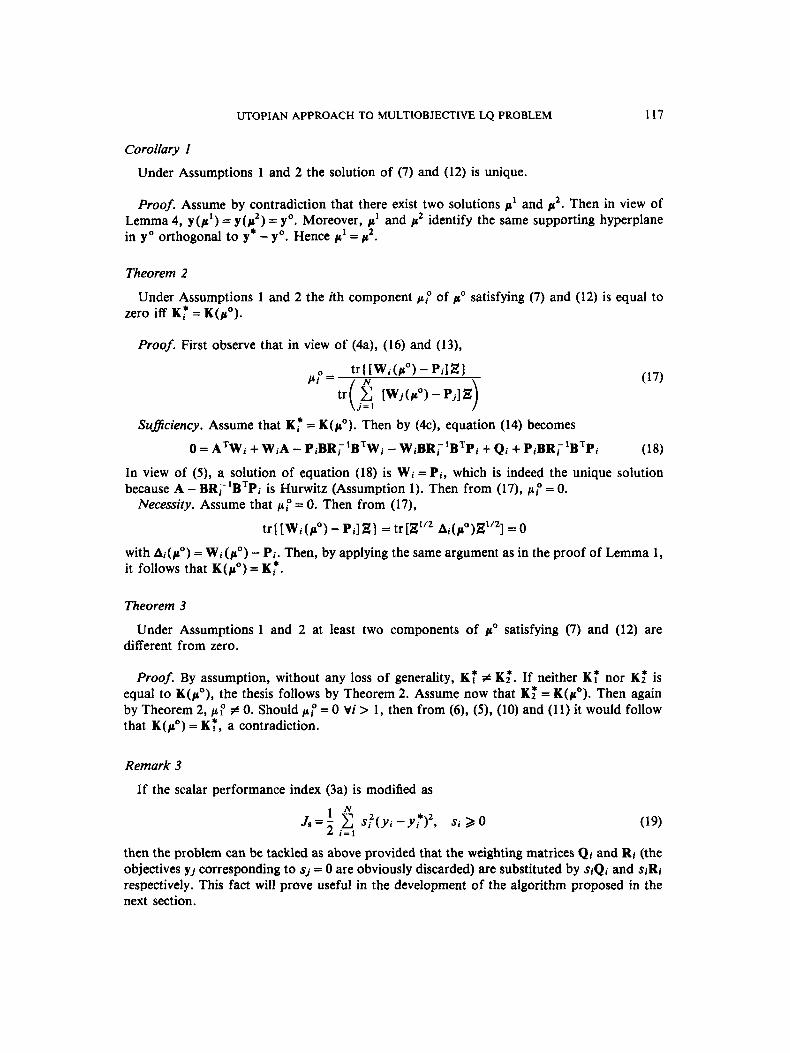
Coroiiary I
Under Assumptions 1 and 2 the solution of (7) and (12) is unique.
Proof. Assume by contradiction that there exist two solutions p1 and p2. Then in view of Lemma 4, y(p') = y(p2) = yo. Moreover, p1 and p2 identify the same supporting hyperplane in yo orthogonal to y* - yo. Hence p1 = p2.
Theorem 2
zero iff K f = K ( p o ) . Under Assumptions 1 and 2 the ith component pp of po satisfying (7) and (12) is equal to
Proof. First observe that in view of (4a), (16) and (13),
Suflciency. Assume that K f = K(po). Then by (4c), equation (14) becomes
0 = ATWi + WiA-PjBR;'B'Wj - WjBRF'BTPi + Qi + PjBRF'BTPi (1 8) In view of (9, a solution of equation (18) is Wi = Pi, which is indeed the unique solution because A - BRF'BTPj is Hurwitz (Assumption 1). Then from (17), pp = 0.
Necessity. Assume that pp = 0. Then from (17),
tr{ [Wi(po) - Pi] Z ) = tr [Z'/2 Ai(po)Z'/2] = 0
with Ai(po) = Wi(po) - Pi. Then, by applying the same argument as in the proof of Lemma 1, it follows that K(po) = K,*.
Theorem 3
different from zero. Under Assumptions 1 and 2 at least two components of po satisfying (7) and (12) are
Proof. By assumption, without any loss of generality, K: # K:. If neither K: nor K: is equal to K ( p o ) , the thesis follows by Theorem 2. Assume now that K: = K(po). Then again by Theorem 2, p P # 0. Should pp = 0 vi > 1, then from (6), (9, (10) and (1 1) it would follow that K(fio) = K:, a contradiction.
Remark 3
If the scalar performance index (3a) is modified as
then the problem can be tackled as above provided that the weighting matrices Qi and Ri (the objectives yj corresponding to sj = 0 are obviously discarded) are substituted by siQi and siRi respectively. This fact will prove useful in the development of the algorithm proposed in the next section.

118 G . DE NICOLAO AND A. LOCATELLI
4. COMPUTATIONAL ASPECTS
In this section we focus on the computation of the optimal solution of the multiobjective optimization problem stated in Section 2. For this purpose, some of the results of the previous section are suitably reviewed.
1. Under Assumptions 1 and 2 the solution (in the utopian sense) to the multiobjective optimization problem exists.
2. The Pareto optimal solutions are parameterized in terms of a vector p which satisfies (7) and the value of y which minimizes (3a) is achieved in correspondence with the unique po that solves equation (12).
3. The relative weight of objectives yi within the global performance index may be varied by suitably choosing the scalars Si in the cost function Js (equation (19)).
In view of these properties, we look for a solution to equation (12) by means of a Newton-' based method, taking into account the constraint (7). As is well known, the Newton method for the solution of a non-linear equation guarantees convergence provided that the initial guess is sufficiently close to the solution. A possible way to exploit such a property relies on the following 'small-step strategy'. Assume that the k-objective problem has been solved (Si = 1, i = 1, ..., k; si = 0, i = k + 1, ..., N , in equation (19)), leading to a vector p(k)o . Then consider the (k + 1)-objective problem in which the (k + 1)th objective is introduced with a sufficiently small weight E (si = 1, i = 1, ..., k; s k + l = E; si = 0, i = k + 2, ..., N , in equation (19)). The solution of this problem is associated with a vector pCk+l ) (e ) that tends to pCk)" for E + 0. In other words, the solution C ' ~ + ' ) ( E ) of equation (12) for the (k+ 1)-objective case (with s k + ] = E ) is close to the solution p(k )o of equation (12) for the k-objective case provided that E is sufficiently small. Therefore p(k )o is a good starting point for solving equation (12) in the (k+ 1)-objective case. By following the same rationale, one can give a sufficiently small increment E' to the weight associated with the (k + 1)th objective ( s k + l = E + E ' ) . Then c ( ~ + ' ) ( E ) is a good starting point for computing pCk+' ) (e + e'). The (k + 1)th objective is then fully incorporated by solving a sequence of (k + 1)-objective problems characterized by Si = 1, i = 1, ..., k, and si = 0, i = k + 2, ..., N, with sk+ progressively approaching unity.
The procedure outlined above can be fruitfully exploited in solving equation (12) for the N-objective case provided that the solution to equation (12) for the two-objective case is made available. As a matter of fact, such a solution can be efficiently computed through a bisection procedure. In fact, letting
1 fl(P1, ..., P N )
fN(PIs - * - P N )
f (p )= [ i ] = p - N [Y (c) - Y*l C [Ui(c)-Y?I
i = 1
it is easily seen that in the two-objective case ( N = 2) f~ (PI, p2) + f 2 ( p 1 , p2) = 0, while owing to (7), 11.2 = 1 - p l . Then the problem is reduced to finding the (unique, by Corollary 1) zero of fl(p1,1 - P I ) in the interval [0,1].
Concerning the order of introduction of the objectives, it does not seem possible to go beyond heuristically based criteria. A possible simple choice is to introduce the objectives according to the increasing magnitude of y(ei) - y*, where ei is the ith column of the N x N identity matrix. Notice that 1 ) y(ei) - y* 1 1 measures the 'loss of performance' (with respect to the utopian point) entailed by the adoption of the control law Ki* (optimal for the ith objective). Hence such ordering is expected to facilitate the 'small-step strategy' outlined above. This way of doing has proven to be effective in a number of examples. Concerning its

UTOPIAN APPROACH TO MULTIOBJECTIVE LQ PROBLEM 119
actual implementation, some minor variants may be required; they are not reported herein since they belong to the customary repertoire of numerical ingenuities.
According to the Newton method for solving f (p) = 0, the basic iteration is
For the problem at hand, the major computational task involved in performing an iteration consists of evaluating the gradient of y in correspondence with the current value of p. Recalling (13), this amounts to efficiently computing
a tr[Wj(C)Zl
taking into account equations (14), (8) and (9). By exploiting well-known results, l 2 one has
aclk
where (recall (8), (6) and (14))
A(p) and Lj(p) being the (unique) solutions of
[A+BK(p)]A+AIA+BK(p)IT+Z=O
[A + BK(k)] TLj + Lj [A + BK(p)] + Zj(p) = 0
with
Z j ( p ) = Zlj(p) + Zlj(p)' + ZU(P) + z 2 j ( ~ ) ~ Z l j ( t ) = - B R ( P ) - ' B ~ w ~ ( P ) A ( c ) ZZj(c0 = -BR(p)-'RjK(p)A(p)
Therefore, when considering k objectives, the computational effort involved at each iteration basically consists of solving
(i) the algebraic Riccati equation (9) (ii) k algebraic Lyapunov equations (14)
(iii) the algebraic Lyapunov equation (20) (iv) k algebraic Lyapunov equations (21) (v) the inversion of [ a f ( p ) / a ~ ] , , = ~ , ~ .
According to a very popular algorithm for solving Lyapunov equations, l 3 a significant amount of computation is devoted to the calculation of the Schur form of the coefficient matrix. Since the coefficient matrices of the Lyapunov equations involved in points (ii)-(iv) are always A + BK(p) or its transpose, the Schur form needs to be computed just once. l4 A further saving in computing the matrices Wi and Lj can be accomplished by exploiting the relations
N
i = l C p i W i = P
120 G . DE NICOLAO AND A. LOCATELLI
which was first derived by Li,’ and
whose correctness is straightforwardly verified. In conclusion, the proposed algorithm consists of the following steps.
1. Order the objectives. 2. Solve (by bisection) the two-objective problem and set k = 3. 3. Select a suitably small weight E for the kth objective and let sk = E.
4. Solve (by Newton) equation (12) for the k-objective problem with the current value of Sk.
5 . If Sk < 1, increment Sk and go to step 4; else, if k # N, go to step 3 with k = k + 1; else
Concerning the computational effort, observe that the solution of a Lyapunov l 3 or Riccati l4
equation requires O(n3) operations. Now, the algorithm is composed of two main parts. The first one solves a two-objective problem by a bisection procedure and its complexity is proportional to O(n3) times a term depending on the number of required iterations. The second part exhibits a three-level nested structure. The outer loop has to do with the number of objectives and is therefore iterated N - 2 times. The middle loop is the ‘small-step iteration’ that leads the weight sk from E to unity. The inner loop performs the basic iteration of the Newton algorithm. Such a basic iteration requires O(kn 3, operations. Therefore the complexity of the second part of the algorithm is at least O(N2n3).
stop.
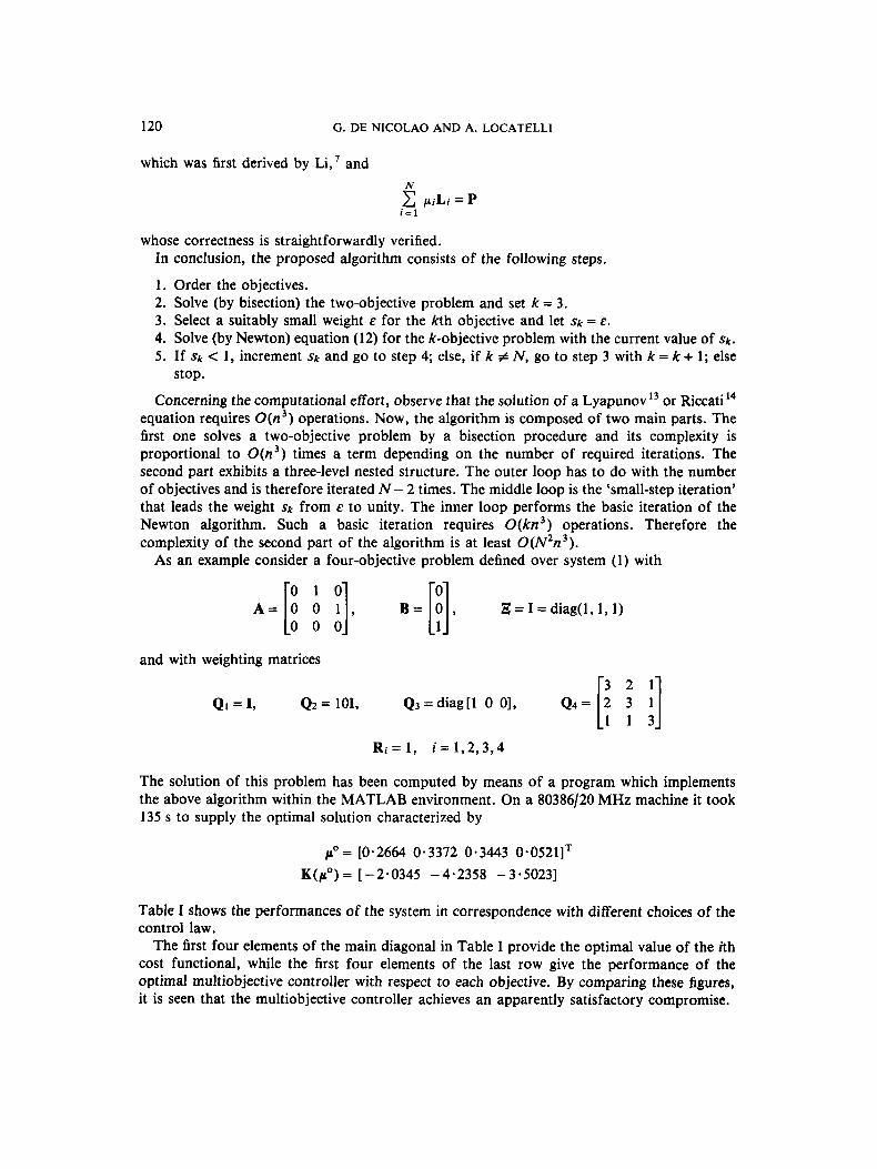
As an example consider a four-objective problem defined over system (1) with
A=[: 0 1 : i], .-[3 Z = I = diag(1, 1 , l ) 0
and with weighting matrices
3 2 1 QI = I, Q2 = 101, Q3 = diag[l 0 01, Q4= [: i]
R i = l , i=1,2,3,4
The solution of this problem has been computed by means of a program which implements the above algorithm within the MATLAB environment. On a 80386/20 MHz machine it took 135 s to supply the optimal solution characterized by
p’ = [0.2664 0.3312 0.3443 0-0521IT K(po)= [-2.0345 -4.2358 -3.50231
Table I shows the performances of the system in correspondence with different choices of the control law.
The first four elements of the main diagonal in Table I provide the optimal value of the ith cost functional, while the first four elements of the last row give the performance of the optimal multiobjective controller with respect to each objective. By comparing these figures, it is seen that the multiobjective controller achieves an apparently satisfactory compromise.

UTOPIAN APPROACH TO MULTIOBJECTIVE LQ PROBLEM 121
Table I. Performances corresponding to different control laws
Performance index Control law Y1 Y2 Y3 Y4 J
K: 4.8284 31.9883 3-6213 8.1569 37-4979 K: 6.7236 25.8895 5.6440 8.6480 9-2431 K: 5.ooOO 34.2500 3.5000 8.5000 70.7005 K: 5.1378 27.9458 3.9429 7.6210 4.5202 K ( P O ) 5.4932 26.7309 4.3591 7.7507 1.9049
5. CONCLUDING REMARKS
In this paper the infinite horizon, continuous time LQ multiobjective problem has been considered and its optimal solution in the utopian sense has been characterized. In particular, it has been shown that the optimal solution always exists and can be efficiently computed by means of the algorithm given in Section 4. The problem considered here can be stated in the finite horizon context as well. Necessary conditions for optimality can easily be obtained via the maximum principle; interestingly enough, they again require the solution of an equation which is nothing but equation (12) written in a finite horizon context. The utopian approach to LQ multiobjective problems has been considered previously in the discrete time, finite horizon case. *' Although the global performance index adopted by Koussoulas and Leondes" is the discrete time counterpart of (3), their discussion turns out to be correct with reference to a different performance, namely
N
i = l J = C (Ui-y: )
(In Reference 11 equation (12) is inconsistent with respect to equation (6).) This is not a minor difference, since this kind of global performance index allows one to skip
the entanglements arising from our equation (12). Indeed, the linearity of J with respect to yi allows one to supply an explicit expression for the optimal p.
A small yet meaningful variant of the problem discussed here consists of considering a constrained multiple-objective optimization problem in which an upper bound is set on one or more performance indices yj . In this way the deterioration of some assigned components of the vector y with respect to the utopian point y* will be kept below a given threshold.
Finally, it is worth mentioning that the dual of the multiobjective LQ control problem may be of some interest in designing Kalman filters when, in place of a unique uncertainty model (namely matrices Q and R characterizing process and output noise variance), a number of likely models (Qi, Ri) are available. This would help in the implementation of robust filters that behave satisfactorily with respect to a number of uncertainty models.
ACKNOWLEDGEMENTS
This paper has been supported by MURST Project 'Model Identification, Systems Control, Signal Processing' and Centro di Teoria dei Sistemi of the CNR, Milano, Italy.

122 G. DE NICOLAO AND A. LOCATELLI
APPENDIX
Proof of Lemma 1
assume by contradiction that for some p First observe that by optimality, Yi(p) -y* >, 0 for all p satisfying (7) and for all i. Now
N
This implies that for each i , vi(p) - y : = 0, i.e.
t r ( [ W i ( p ) - P i J Z ] = tr[Z''2 Ai(p)Z"*] = O (22)
with Ai(p) = Wi(p) -Pi. By optimality, Ai(p) >, 0, SO that equation (22) implies Ai(p) = 0, i.e.
Wi ( p ) = Pi (23) Now consider the matrix function
Z(K) = (A + BK)TPi + Pi(A + BK) + Qi + KTRiK
Letting K = K: + 6K and exploiting equations (4c) and (3, we have
Z(K) = GKTRi 6K
Hence Z(K) = 0 iff 6K = 0, i.e iff K = K:. From (14) and (23) it follows that Z(K(p)) = 0 and hence K f = K ( p ) Vi. In particular, this happens for the pair ( h , j ) which, according to Assumption 2, is such that Kh+ # Kf , a contradiction.
Proof of Lemma 3
In order to proceed, we need some definitions. Let
1 f ( p ) = p - N [Yb) - Y*l
C [ri(p)-Yi*l i = l
I k
~ k = ~ : ~ E I R ~ , v ~ > , o , I < ~ Q ~ , C q i = 1 , I Q ~ Q N I i = l
From now on, pk will denote a generic element of Mk. Moreover,
l Q k Q N - 1
a k + ' ( C k ) : h fk [o, 11, 1 Q k < N - 1 (24) p k + l , k ( p k ) = p k + l ( a k + ' ( p k ) , p k ) , 1 < k Q N - 1
pNs k ( p k ) = pN, N- 1 (pN- 1, N-2 ( . . . ( p k " * k ( p k ) ) ) ) , 1 Q k Q N- 1
Expression (24) introduces a set of functions a k ( - ) that will be suitably defined in the following.
The main idea behind the proof consists of progressively reducing the dimensionality through an iterative procedure which at each step increases by one the number of components
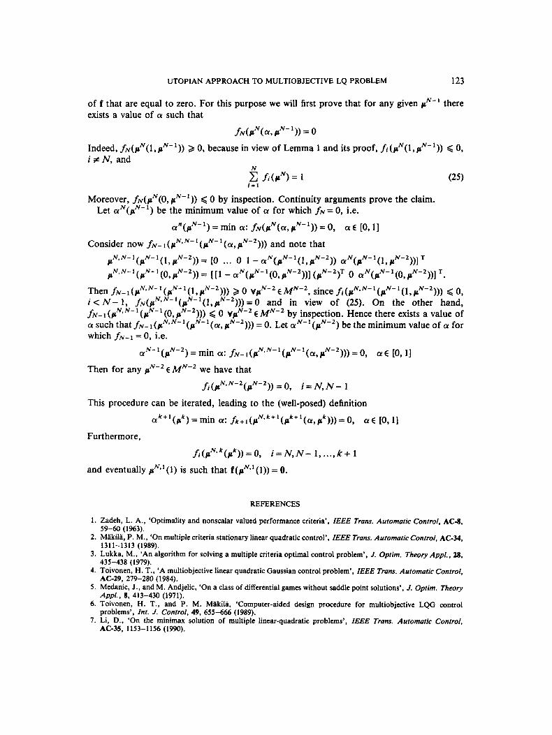
UTOPIAN APPROACH TO MULTIOBJECTIVE LQ PROBLEM 123
of f that are equal to zero. For this purpose we will first prove that for any given p N - l there exists a value of a such that
fN(rN(a. p N - 1) = 0
Indeed, fN(pN(l,pN-l)) 2 0, because in view of Lemma 1 and its proof, f i ( p N ( 1 , p N - ’ ) ) < 0, i # N, and
N
i = l C f i ( p N ) = 1 (25)
Moreover, fN(pN(O, p N - ’ ) ) < 0 by inspection. Continuity arguments prove the claim. Let a N ( p N - ’ ) be the minimum value of a for which fN = 0, i.e.
an (pN-1 ) = min a: fN(pN(a, p N - l ) ) = 0, a c [O, 1 1
Consider now fN-l(rCN’N-l(PN-’(CY, pN-2 ))) and note that p”N-l (pN-1(1,pN-2))= [0 ... 0 1 - a N ( p N - 1 ( l , p N - 2 ) ) a N ( p N-1 ( 1 , p N - 2 ) ) 1 T
c N.N-l(pN-l(O,pN-2)) = [ [ l - aN(pN- l (O ,pN-2) ) ] (pN-2)T 0 aN(pN-I (0, pN-2))1 T .
Then fN- 1 ( p N s N - ’ ( p N - ’ ( 1, p”-’))) 2 0 VpN-2 C MN-2 , since fi ( p N S N - ( p N - (1, pN-’)>) < 0, i < N - l , fN(P N’N-1(pN-1(l,pN-2)))=0 and in view of (25). On the other hand, fN- (pNsN-’ (pN-’ (0, pN-’)>) < 0 ~ p ~ - ~ € MN-’ by inspection. Hence there exists a value of
be the minimum value of a for which fN-l= 0, i.e.
such that fN- (pN-N-’(pN-l(a, pN-’))) = 0. Let
aN-’(pN-‘)=min a: fN-I(pN,N-1(pN-1(a,pN-2)))=~, a € [o, 1 1 Then for any pN-2 E MN-2 we have that
f i ( p N * N - 2 ( p N - 2 ) ) = 0, i = N, N - 1
This procedure can be iterated, leading to the (well-posed) definition
ak+l(pk)=min a: fk+ l (pN,k+ l (pk+ ’ (a ,pk ) ) )=O, [o, 1 1
Furthermore,
f i ( p N ” ( p k ) ) = O , i = N , N - 1 , . . . , i t + 1
and eventually p N * ’ ( l ) is such that f(pNP1(l)) = 0.
REFERENCES
1. Zadeh, L. A., ‘Optimality and nonscalar valued performance criteria’, IEEE Trans. Automatic Control, AC-8,
2. Makila, P. M., ‘On multiple criteria stationary linear quadratic control’, IEEE Trans. Automatic Control, AC-34, 59-60 (1963).
13 1 1- 13 13 (1989). 3. Lukka, M., ‘An algorithm for solving a multiple criteria optimal control problem’, J. Optim. Theory Appl., 28,
435-438 (1979). 4. Toivonen, H. T., ‘A multiobjective linear quadratic Gaussian control problem’, IEEE Trans. Automatic Control,
5 . Medanic, J., and M. Andjelic, ‘On a class of differential games without saddle point solutions’, J. Optim. Theory
6. Toivonen, H. T., and P. M. Makila, ‘Computer-aided design procedure for multiobjective LQG control
7. Li, D., ‘On the minimax solution of multiple linear-quadratic problems’, IEEE Trans. Automatic Control,
AC-29, 279-280 (1984).
Appl., 8, 413-430 (1971).
problems’, Znt. J. Control, 49, 655-666 (1989).
AC-35, 1153-1156 (1990).

124 G. DE NICOLAO AND A. LOCATELLI
8. Salukvadze, M. E., ‘Optimization of vector functionals. I. The programming of optimal trajectories’, Automatics
9. Salukvadze, M. E., ‘Optimization of vector functionals. 11. The analytic construction of optimal controls’,
10. Li, D., ‘A new solution approach to Salukvadze’s problem’, Proc. Am. Control Con$, San Diego, CA, 1990,
11. Koussoulas, N. T., and C. T. Leondes, ‘The multiple linear quadratic Gaussian problem’, Int. J. Control, 43,
12. Kwakernaak, H., and R. Sivan, Linear Optimal Control Systems, Wiley-Interscience, New York, 1972. 13. Bartels, R. H., and G. W. Stewart, ‘Solution of the matrix equation A X + XB = C, Commun. ACM, 15,
14. Kleinman, D. L., and P. Krishna Rao, ‘Extensions to the Bartels-Stewart algorithm for linear matrix equations’,
15. Laub, A. J., ‘A Schur method for solving algebraic Riccati equations’, IEEE Trans. Automatic Control, AC-24.
Telemech., 8. 5-15 (1971).
Automatics Telemech., 9, 5-15 (1971).
pp. 409-414.
337-349 (1986).
820-826 (1972).
IEEE Trans. Automatic Control, AC-23, 85-87 (1978).
913-921 (1979).