Journal of Forecasting, Vol. 12, 239-253 (1993)

On the Use of Dispersion Measures from NAPM Surveys in Business Cycle Forecasting

SUSMITA DASGUPTA and KAJAL LAHlRl State University of New York, Albany, NY, U.S.A.

ABSTRACT

Qualitative survey data on changes in production, inventory, new order, and employment collected every month by the National Association of Purchasing Managers are analysed over 1948-90. The Probability method we use generates time-series estimates of cross-section variabilities across firms. It is shown that these digusion measures have additional explanatory power in the prediction of business cycle turning points.

KEY WORDS Purchasing managers’ survey Qualitative response Sectoral variability Inventory dispersion Cyclical turning point

INTRODUCTION

In recent years several economists have found business surveys conducted by the National Association of Purchasing Managers (NAPM) to be useful in tracking short-run cyclical fluctuations. Torda (1985a, b) of the US Department of Commerce has combined five key NAPM indicators into a composite index. Klein and Moore (1991) also concluded that these data are useful in monitoring the ebb and flow of the business cycle. Niemira (1986) has used the buying price index as one of the components in the Paine-Webber composite inflation indicator. The movement of the NAPM index is reported regularly by the popular press in the USA and attracts considerable public attention every month.

The NAPM surveys, like many others around the world, are qualitative in the sense that each respondent is asked to answer whether the variable has gone ‘up’, ‘down’, or ‘stayed the same’ during the last month. Most studies, including those at the US Department of Commerce, use diffusion indexes of some form, such as the percentage of industries experiencing an ‘increase’ plus half the percentage saying ‘no change’. This diffusion index is actually a simple linear function of the so-called ‘balance’ statistic, due to Anderson (1952) and Theil (1952), which is obtained by subtracting the percentage saying ‘down’ from the percentage saying ‘up’. It can be shown that the balance statistic is a measure of rate of change in the underlying variable (see Pesaran, 1988). Oller (1990) has demonstrated that the ‘balance’-related statistics derived from qualitative surveys can track turns in economic variables much better than automated time-series models. 0277-6693 /93/030239- 1 5$12.50 Received September 1991 0 1993 by John Wiley & Sons, Ltd. Revised July 1992

240 Journal of Forecasting Vol. 12, Zss. Nos. 3 & 4

Carlson and Parkin (1975) have extended the probability approach of Anderson (1952) and Theil (1952) by reparameterizing the data in a more helpful form such that mean and variance of the underlying aggregate distribution can be calculated. On the assumption that individual responses represent independent drawings from this aggregate distribution, the variability can also provide us with a direct measure of dispersion of actual change in a variable across firms. There are some studies which have examined the role of inflation variability on real economic variables.’ However, very little empirical work has been devoted to study the effect of variability in real economic variables (e.g. employment, inventories, etc.) across firms on the propagation of business cycles, even though some authors like Lilien (1982), Loungani and Rogerson (1989), and others have argued that employment variability due to sectoral shifts have important macroeconomic implications.

The main purpose of the present paper is to analyse cross-sectional variabilities in production, inventories of purchased materials, new orders, and employment estimated from NAPM business survey data and to explore their potential for economic forecasting. We have found that these series have independent power to explain variations in such variables as industrial production, unemployment, and real GNP. In this paper we have paid special attention to the performance of inventory dispersion in predicting NBER business cycle turns.

The plan of the paper is as follows. The next section contains the statistical framework to estimate cross-sectional variability from the three-category qualitative survey data. The possible use of these dispersion series to forecast different macroeconomic variables is given in the third section. The fourth section examines the potential of NAPM variability /dispersion data for business cycle turning-point prediction. Conclusions are summarized in the final section.

THE STATISTICAL FRAMEWORK

Let us posit that the perceived rate of change in the key survey item for the ith respondent (market) at time t can be decomposed into two unobserved components:

gi*1= pt + t i t

where p t is the economy-wide average and t i r is the firm-specific disturbance term with E(tit) = 0 and E ( t f r ) = a?. Individual firms have problems decomposing g ; into economy-wide growth rate, p t , and firm-specific disturbance, t i t . As econometricians, however, we have visited M markets and are in a position to estimate p t and a:. It is assumed that respondents answer ‘up/same/down’ according as 6 i t < git , - 6 i g < gi*1 < 6 i t and g : < - 6 i t . Here Sir is the just-noticeable difference (j-n-d) in the rate of change of the key variable or the imperceptible threshold. Note that with lower values of at, an econometrician will be able to estimate pt more precisely (see Grossman, 1983).

If At, Bt, Ct, respectively, are the probabilities that the perceived rate of change was ‘up’, ‘same’, ‘down’, then

*

and

’See Lahiri er ul. (1988) and references therein.

S. Dasgupta and K . Lahiri NAPM Surveys in Business Cycle Forecasting 241

where F( . ) is the cumulative distribution of & i t . Given a distributional assumption for &it , these equations can be solved to obtain estimates of the parameters. However, the survey response proportions are not sufficient to identify all the parameters of interest. We can get estimates of pt and ut provided we have an estimate of just-noticeable-difference, 6ir. Carlson and Parkin (1975) assumed that the thresholds 6 i t are equal across respondents and constant over time, i.e. 6 i t = 6 for all i , t . They also made the assumption that &it is normally distributed.

Following them, if we make the assumption of normal distribution and define F(at) = 1 -At , F(ct) = Ct then it follows that af = (6 - pt)/ut and cf = (- 6 - pt) /ut . Solving these two equations we get:

at + ct p t = 6 - ct - at

and

- 2 ut=6---

ct - at

(4)

Once the distributional assumption is made, (at c t ) can be readily calculated from sample proportions (At Cr). An estimate of at will be denoted by st.

The problem of getting an estimate of 6 is tackled by Carlson and Parkin (1975) by the assumption of long-term unbiasedness so that

c gt E(at + ct) / (c t - at ) (6)

where gt is the observed, actual rate of change of the key variable at time t . Note that equation (6) does not yield unbiased estimates in the statistical sense, i.e. E ( p t ) # g t . Alternatively, 6 can be estimated by regressing gf through the origin on unscaled estimates, that is, by imposing the statistical unbiasedness condition (see Batchelor, 1982).

Many researchers have criticized the Carlson-Parkin (C-P) method primarily due to the scaling procedure (see Batchelor and Orr, 1988; Pesaran, 1988; Visco, 1985). However, in the present context the scaling technique as given in equation (6) or Batchelor (1982)’s statistical unbiasedness condition makes good sense. First, unlike expectational surveys, NAPM data are about perceived actual rate of change of a variable. Empirical evidence suggest that perceptions are, in general, unbiased (see Jonung and Laidler, 1988). Second, the NAPM question is regarding rate of change of a variable for the particular firm which employs the respondent. We can assume that each respondent knows what is happening to his or her own company, and reports accordingly. Third, the rate of change is over the immediate past month and not over a whole year. Thus, the response by each participant should be informationally less taxing.

The assumption of symmetric indifference interval can be easily relaxed. Following Seitz (1988), let us assume that respondents answer ‘up/same/down’ according as < g z , SL c g: < 6’ and g z < tiL, where 6’ and 6 L are, respectively, the upper and lower limits of imperceptibility. Using equations (2) and (3), at and ct can be rewritten as ar = (6‘ - pt) /ut and ct = (SL - pt)/ut, and hence

6 =

and

242 Journal of Forecasting Vol. 12, Zss. Nos. 3 & 4

By imposing statistical unbiasedness on equation (4a), 6" and hL can be estimated. Using equation (sa), ut can then be obtained.

Many researchers have found the normality assumption unrealistic. Carlson (1 977) and Lahiri and Teigland (1983) discovered that the scaled t-distribution is a good alternative. Following Praetz (1972) and Kawasaki et al. (1983), we can assume that g: has a scaled t-distribution, i.e.

t* = ( v / v - l)1/2(g: - pr)/ur

at = ( v / v - 1)'/2(6 - pr)/ut

Cf = ( v / v - 1 Y 2 ( - 6 - po/ut

(7) where 1 is the degrees of freedom parameter. Then it follows that

and

where at and ct are the t-values which cut off A, and Ct in the upper and lower tails, Then two equations can be solved for pt and sr as

pt = + cr)/(at - ct) (4b)

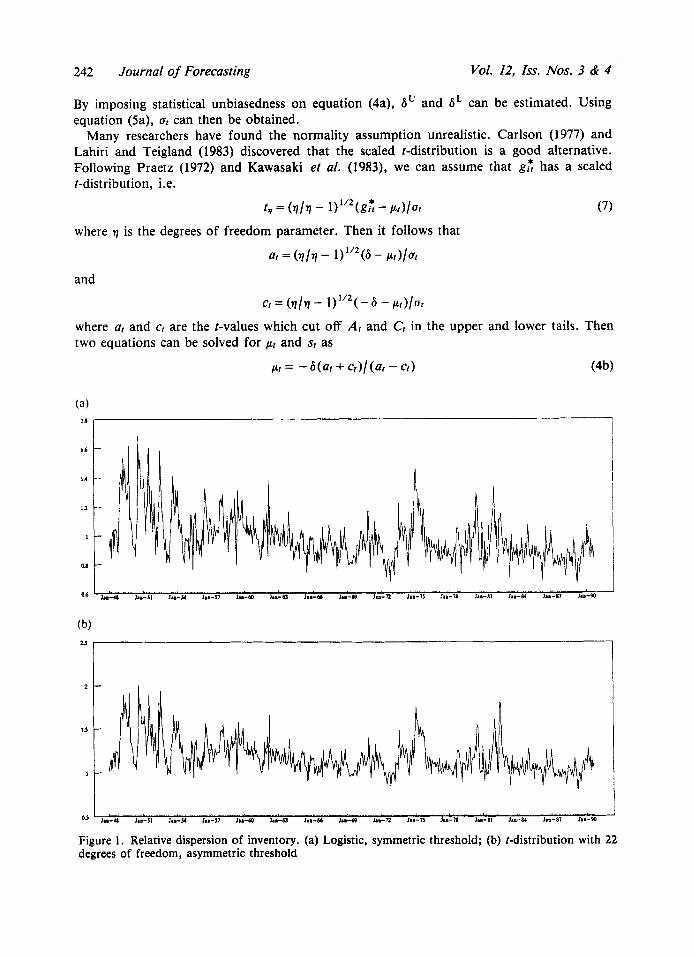
Figure 1 . Relative dispersion of inventory. (a) Logistic, symmetric threshold; (b) t-distribution with 22 degrees of freedom, asymmetric threshold

S. Dasgupta and K. Lahiri NAPM Surveys in Business Cycle Forecasting 243

and 6, = - 26(.rl/.rl - 1) '"/(ct - at) (5b)

The degrees of freedom parameter, 7, can be estimated by estimating the model over different values of 77 and choosing the value of 9 which yields minimum mean square errors. In our experiments, the optimal value of 7 was 22.

The estimates of relative dispersion of employment, production, new order, and inventory derived from NAPM data are estimates of inter-firm variability in the manufacturing sector. It should be recalled, however, that the respondents of the NAPM survey are scattered over separate markets, and, as a result, each respondent only observes and replies to the survey question in light of the conditions prevailing in his or her firm. Consequently, low relative dispersion estimates imply smaller inter-firm variation. Thus, these dispersion estimates are truly measures of 'diffusion' in the manufacturing sector along several dimensions.

Using alternative assumptions about distribution and the threshold parameter, we estimated at from NAPM business survey data for the manufacturing sector. Our implementation of the C-P procedure produced strikingly similar estimates of dispersion for normal and scaled t-distributions with different degrees of freedom. Estimates of symmetric and asymmetric j-n-d parameters were also remarkably alike (see Figure 1). Thus, in this paper we shall report estimates derived from normal distribution with symmetric j-n-d parameter.

PREDICTIVE POWER OF NAPM DISPERSION MEASURES

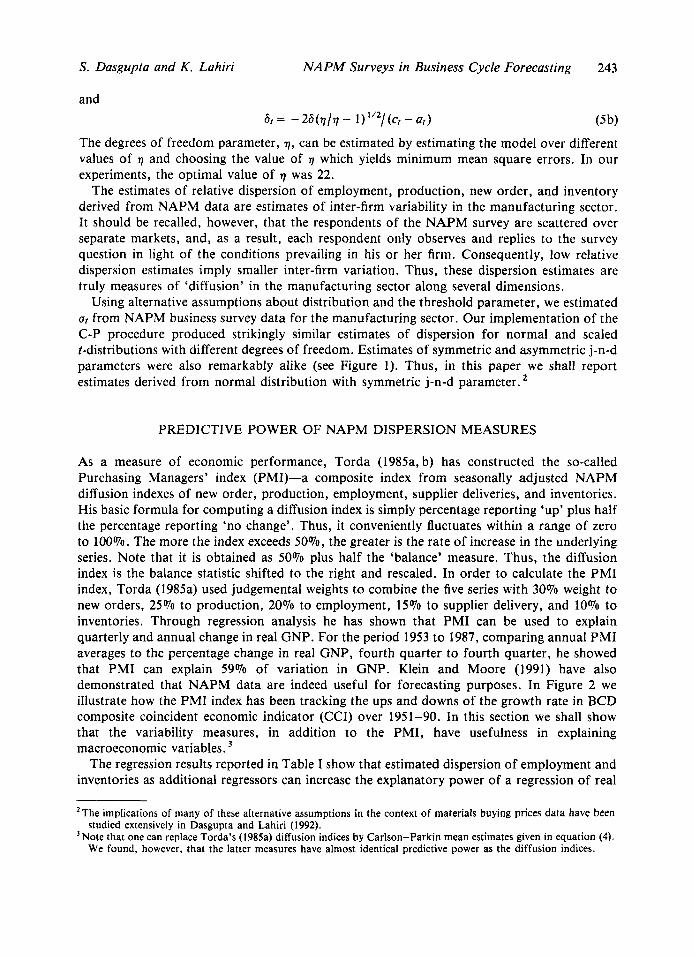
As a measure of economic performance, Torda (1985a, b) has constructed the so-called Purchasing Managers' index (PM1)-a composite index from seasonally adjusted NAPM diffusion indexes of new order, production, employment, supplier deliveries, and inventories. His basic formula for computing a diffusion index is simply percentage reporting 'up' plus half the percentage reporting 'no change'. Thus, it conveniently fluctuates within a range of zero to 100%. The more the index exceeds 50%, the greater is the rate of increase in the underlying series. Note that it is obtained as 50% plus half the 'balance' measure. Thus, the diffusion index is the balance statistic shifted to the right and rescaled. In order to calculate the PMI index, Torda (1985a) used judgemental weights to combine the five series with 30% weight to new orders, 25% to production, 20% to employment, 15% to supplier delivery, and 10% to inventories. Through regression analysis he has shown that PMI can be used to explain quarterly and annual change in real GNP. For the period 1953 to 1987, comparing annual PMI averages to the percentage change in real GNP, fourth quarter to fourth quarter, he showed that PMI can explain 59% of variation in GNP. Klein and Moore (1991) have also demonstrated that NAPM data are indeed useful for forecasting purposes. In Figure 2 we illustrate how the PMI index has been tracking the ups and downs of the growth rate in BCD composite coincident economic indicator (CCI) over 1951-90. In this section we shall show that the variability measures, in addition to the PMI, have usefulness in explaining macroeconomic variables.

The regression results reported in Table I show that estimated dispersion of employment and inventories as additional regressors can increase the explanatory power of a regression of real

'The implications of many of these alternative assumptions in the context of materials buying prices data have been studied extensively in Dasgupta and Lahiri (1992).

'Note that one can replace Torda's (1985a) diffusion indices by Carlson-Parkin mean estimates given in equation (4). We found, however, that the latter measures have almost identical predictive power as the diffusion indices.

244 Journal of Forecasting Vol. 12, Iss. Nos. 3 & 4

80 T----- 4

60

2

40

0

20 - 2

* C C I - PMI

Jan 151152153154155156157~58~59160(61162(63164~65~66~67~66~69~70~ 5 1 ~ 7 2 ~ 7 3 ~ 7 4 ~ 7 5 ~ 7 6 ~ 7 7 1 7 8 1 7 9 1 8 0 1 8 1 ~ 8 2 ~ 8 3 ~ 8 4 ~ 8 5 ~ 6 6 ~ 8 7 ~ s s l e s k d

Figure 2. Purchasing managers’ index versus coincident indicator

GNP growth on PMI very significantly. The increase in R2 is between 10% and 20%. We also explored the possibility of using NAPM variability data to track movement of widely used CCI and composite leading indicator (CLI). Examination of Table I1 reveals that PMI can explain 61% of the quarterly rate of change in BCD Composite Coincident Indicators. However, the Durbin-Watson statistic (1 3 0 ) shows that the residuals are serially correlated. The dispersion measures (of employment, new order, inventories, and production) together with PMI can raise this value to 68% with a significant improvement in serial correlation of residuals. Associated Durbin-Watson of 1.71 is very close to the critical lower bound value 1.72. Similar improvements are also noticeable for CLI.

The informational content of PMI and the proposed dispersion measures in predicting GNP and other economic indicators have also been rigorously tested using the so-called encompassing test, by regressing the variable to be forecasted on its alternative forecasts (see Fair and Shiller, 1989, 1990). As we see in Table 111 (rows 2-5), each dispersion measure, in addition to PMI, contains independent information in explaining real GNP growth. Also, both PMI and changes in CCI have independent information in explaining real GNP growth (row

Table I . Prediction of growth rate of real GNP (1953-86)a

Dependent variable Intercept PMI S L I P ST”” R2 D-W

Quarterly growth rate

Quarterly growth rate

Annual growth rate

Annual growth rate

- 3.887 (-8.313)

- 3.585 (- 3.269)

-13.091 (- 5.529)

-13.321 (-2.519)

0.086 (9.973)

0.42 1.88

0.083 10.177 -8.173 0.52 1.94 (9.001) (4.48) (-4.625)

0.299 (6.821)

0.58 1.99

0.306 32.214 -25.216 0.65 2.32 (6.714) (2.674) (- 2.384)

a t-statistics are in parentheses.

S. Dasgupta and K . Lahiri NAPM Surveys in Business Cycle Forecasting 245

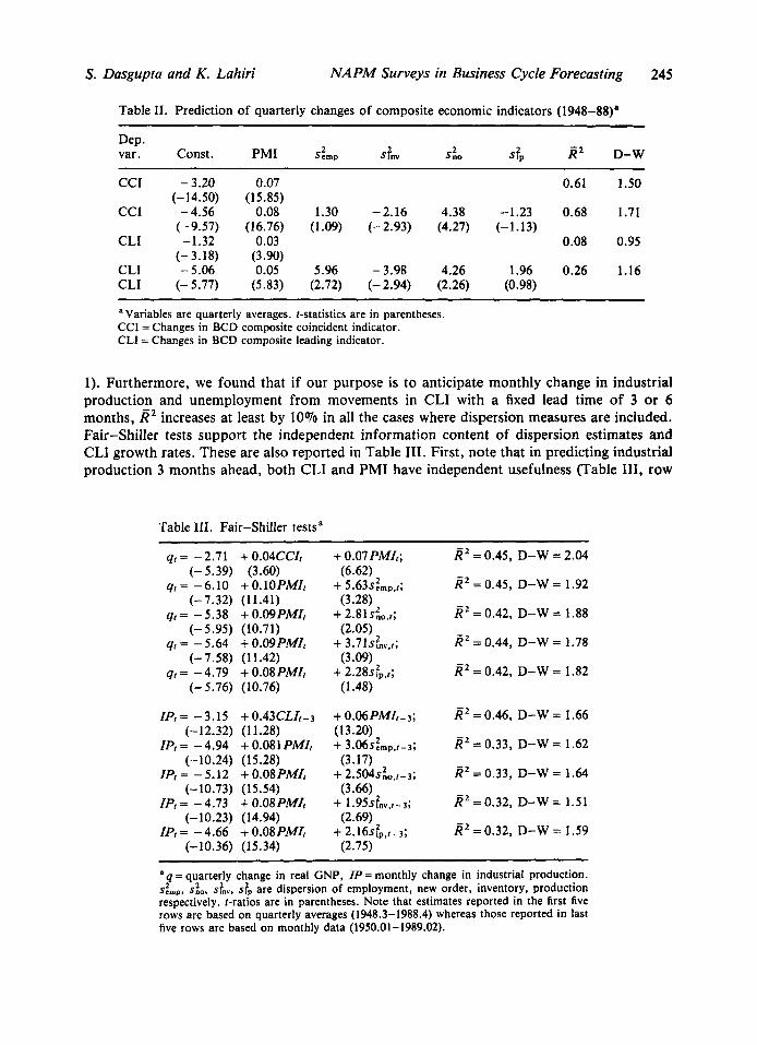
Table 11. Prediction of quarterly changes of composite economic indicators (1948-88)' ~ ~~~

Dep. s tp R 2 D-W 2 2 var . Const. PMI Semp s ?nv Sno

CCI - 3.20

CCI - 4.56 (- 9.57)

CLI -1.32 (- 3.18)

(-14.50)

CLI - 5.06 CLI (-5.77)

0.07 0.61 1.50 (1 5.85)

0.08 1.30 -2.16 4.38 -1.23 0.68 1.71 (16.76) (1.09) (-2.93) (4.27) (-1.13)

0.03 0.08 0.95 (3.90) 0.05 5.96 -3.98 4.26 1.96 0.26 1.16

(5.83) (2.72) (- 2.94) (2.26) (0.98)

a Variables are quarterly averages. &statistics are in parentheses. CCI = Changes in BCD composite coincident indicator. CLI = Changes in BCD composite leading indicator.

1). Furthermore, we found that if our purpose is to anticipate monthly change in industrial production and unemployment from movements in CLI with a fixed lead time of 3 or 6 months, i?' increases at least by 10% in all the cases where dispersion measures are included. Fair-Shiller tests support the independent information content of dispersion estimates and CLI growth rates. These are also reported in Table 111. First, note that in predicting industrial production 3 months ahead, both CLI and PMI have independent usefulness (Table 111, row

Table 111. Fair-Shiller testsa

qt= -2.71 +O.O4CCIt (-5.39) (3.60)

qt= -6.10 +O.lOPMI, (-7.32) (11.41)

(- 5.95) (10.71)

(-7.58) (11.42)

(-5.76) (10.76)

IPt= -3.15 +0.43CLIt-3

41 = - 5.38 + 0.09PMIt

qt = - 5.64 + 0 . 0 9 p ~ r ~

= -4.79 + 0.08PMIt

(-12.32) (11.28)

(-10.24) (15.28) IPt= -5.12 +O.O8PMIt

(-10.73) (15.54)

(-10.23) (14.94) IPt= -4.66 +O.OSPMZt

(-10.36) (15.34)

IPt= - 4.94 + 0.081 PMIt

IPt = - 4.73 + 0.08PMZt

+ 0.07 PMIt;

+ 5.63~:mp~; (6.62)

(3.28)

(2.05)

(3.09)

(1.48)

+ 2.81~:,,~;

+ 3.71~fnv~t;

+ 2.28s$,,;

+ 0.06PMIt-3; (13.20) + 3.06~&,,~,t-3;

(3.17) + 2.504sg0,t-3;

(3.66) + 1.95sfnV,t-3;

(2.69) + 2.16s:p,t-3;

(2.75)

R2 = 0.45, D-W = 2.04

R 2 = 0.45, D-W = 1.92

R2 = 0.42, D-W = 1.88

R2 = 0.44, D-W = 1.78

R 2 = 0.42, D-W = 1.82

R 2 = 0.46, D-W = 1.66

R2 = 0.33, D-W = 1.62

R 2 = 0.33, D-W = 1.64

X 2 =0.32, D-W = 1.51

R 2 = 0.32, D-W = 1.59

a q = quarterly change in real GNP, IP = monthly change in industrial production. S C ~ , , , ~ , do, &., s$, are dispersion of employment, new order, inventory, production respectively. 1-ratios are in parentheses. Note that estimates reported in the first five rows are based on quarterly averages (1948.3-1988.4) whereas those reported in last five rows are based on monthly data (1950.01-1989.02).

246 Journal of Forecasting Vol. 12, Iss. Nos. 3 & 4

6). However, each of the dispersion measures is highly significant after PMI is included in the regression. We obtained very similar results with unemployment rate and with six-month- ahead predictions. These results are not reported here, but can be obtained from the authors. This suggests that the usefulness of PMI and CLI can be significantly enhanced if we include dispersion measures as their components. This empirical finding is consistent with some of the recent developments in real business cycle theory where intersectoral reallocation rather than demand shocks are thought to be the main reason behind business cycles.

TURNING-POINT FORECASTS USING INVENTORY DISPERSION

The prediction of business cycle turning points is one of the most challenging aspects of forecasting in business and economics. Early detection or even timely recognition of turning points has always been a major concern of policy makers, businesses, and investors. Early recognition would allow the economic agents to redo their economic calculations for the forthcoming environment. For many years, system of leading and coincident economic indicators have been widely used in the USA to appraise the state of business cycles. The coincident indicators are comprehensive measures of a nation’s current economic performance, whereas the leading indicators have a ‘look-ahead’ quality.

Leading indicator approach is the typical way of monitoring and forecasting cyclical turning points. This method dates back to 1937 and uses the local maximum (minimum) or other characteristic of a leading index as a signal of an ensuing maximum/minimum in other series of interest. Rate of change of coincident indicator is then used to confirm the turn.4 On the whole, a general lack of success in predicting turning points has been documented by several prominent researchers. Sometimes they miss actual turns and sometimes predicted turns do not occur. To quote Moore (1983, p. 407): ‘The data as a whole suggest that forecasters have yet to establish their ability to detect turning points in aggregate economic activity well in advance of the event.’

We have found that estimates of cross-sectional variability in employment, new order, inventories, production, and supplier deliveries extracted from NAPM survey data can be used to forecast turning points of business cycle with varying degrees of success. In times of steady expansion (contraction) most of the firms will be reporting a rise (fall) in employment, new order, etc. and consequently low a: will be associated with either steady increase or decrease in economic activity. On the other hand, around turning points, markets are in flux. Many firms will experience increases in these key variables side by side with others who may experience decreases. Thus, high a: will prevail in the vicinity of turning points.

Our regression results strongly support this hypothesis. We have found a direct positive relationship between the absolute value of deviation of growth rate of a particular variable from its long-term growth path and cross-sectional variability. The long-term growth path was calculated by retrieving the fitted values from a regression of actual growth rate on a constant, time and time-square. The results are documented in Table IV, where we find that high values of dispersion in employment, inventory, new order, and production are strongly associated with high absolute values of the deviations. This is because we expect historically high s: around both peaks and troughs. Interestingly, this suggests that a string of positive first differences of the s: curves (i.e. a steady rise in the dispersion) following a steady fall and

4See Lahiri and Moore (1991, Chapter 1) for a comprehensive review.

S. Dasgupta and K . Lahiri NAPM Surveys in Business Cycle Forecasting 241

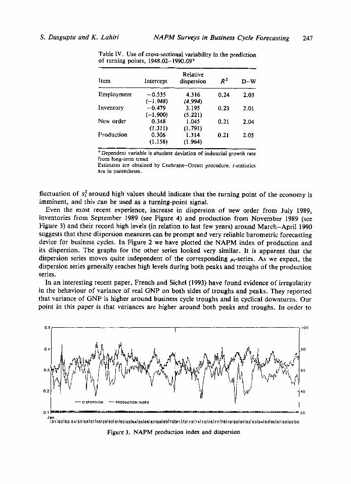
Table IV. Use of cross-sectional variability in the prediction of turning points, 1948.02-1990.09a

Relative Item Intercept dispersion R2 D-W

Employment - 0.535 (-1.948)

Inventory - 0.479 (-1.900)

New order 0.348 (1.311)

Production 0.306 (1.1 58)

4.316 0.24 2.03 (4.994) 3.195 0.23 2.01

1.045 0.21 2.04

1.314 0.21 2.05

(5.22 1)

(1.791)

(1.964)

a Dependent variable is absolute deviation of industrial growth rate from long-term trend Estimates are obtained by Cochrane-Orcutt procedure. t-statistics are in parentheses.

fluctuation of s: around high values should indicate that the turning point of the economy is imminent, and this can be used as a turning-point signal.

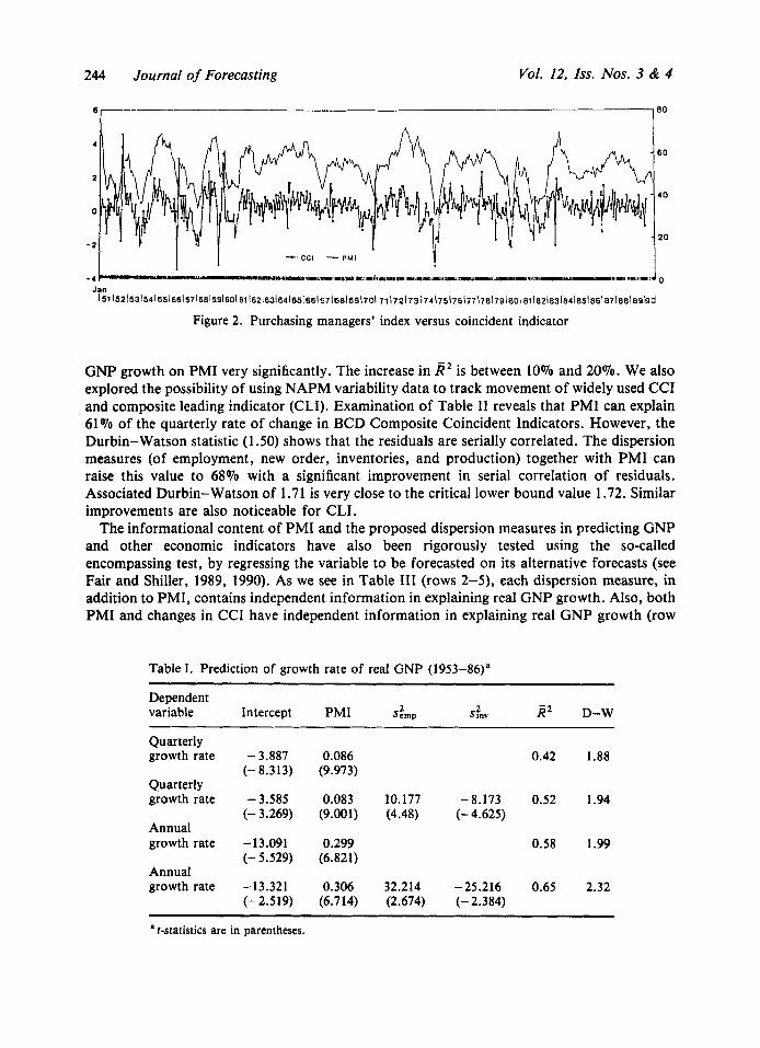
Even the most recent experience, increase in dispersion of new order from July 1989, inventories from September 1989 (see Figure 4) and production from November 1989 (see Figure 3) and their record high levels (in relation to last few years) around March-April 1990 suggests that these dispersion measures can be prompt and very reliable barometric forecasting device for business cycles. In Figure 2 we have plotted the NAPM index of production and its dispersion. The graphs for the other series looked very similar. It is apparent that the dispersion series moves quite independent of the corresponding pt-series. As we expect, the dispersion series generally reaches high levels during both peaks and troughs of the production series.

In an interesting recent paper, French and Sichel (1993) have found evidence of irregularity in the behaviour of variance of real GNP on both sides of troughs and peaks. They reported that variance of GNP is higher around business cycle troughs and in cyclical downturns. Our point in this paper is that variances are higher around both peaks and troughs. In order to

248 Journal of Forecasting Vol. 12, Iss. Nos. 3 & 4

0.6

0.55

0.5

0.45

0.4

0.35

Jan 154 1551 56 I 5 7 1581 59 160 I 61 162 163 164 165 166 167 168 I69 1701 71 1721731 74 1751761771781791801 81 I82183184 185186 187 1881 89190

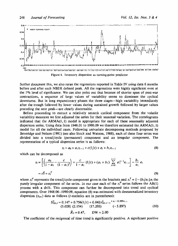
Figure 4. Inventory dispersion as turning-point predictor

further document this, we also reran the regressions reported in Table IV using data 6 months before and after each NBER defined peak. All the regressions were highly significant even at the 1 % level of significance. We can also point out that because of shorter span of post-war contractions, a sequence of large values of variability seems to dominate the cyclical downturns. But in long expansionary phases the three stages-high variability immediately after the trough followed by lower values during sustained growth followed by larger values preceding the next peak-are clearly discernable.

Before proceeding to extract a relatively smooth cyclical component from the volatile variability measures we first adjusted the series for their seasonal variation. The correlograms indicated that the ARMA(1,l) model is appropriate for each of these seasonally adjusted dispersion series. Using data from 1948.01 to 1990.09 we therefore estimated the ARMA( 1, 1) model for all the individual cases. Following univariate decomposing methods proposed by Beveridge and Nelson (1981) (see also Stock and Watson, 1988), each of these four series was divided into a trend/cycle (permanent) component and an irregular component. The representation of a typical dispersion series is as follows:

(8) sr = a0 + al Sr - 1 + c( 1 It) + er + bl er- 1

which can be decomposed as

(9)

where SP represents the trend/cycle component given in the brackets and s,' = [ - (bl/al] er the purely irregular component of the series. In our case each of the sP series follows the AR(1) process with a drift. This component can further be decomposed into trend and cyclical components. Over 1948:06- 1990:09, equation (8) was estimated with deseasonalized inventory dispersion (Sinv) data as follows (t-statistics are in parentheses):

P T = S r + S t

S f n v , f = 0.147 + 0.756(1/t) + (3.028) (2.154) (17.203) (- 5.897) (10)

3 2 = 0.47, DW = 2.00

The coefficient of the reciprocal of time trend is significantly positive. A significant positive

S. Dasgupta and K . Lahiri NAPM Surveys in Business Cycle Forecasting 249

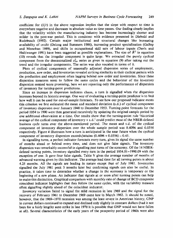
coefficient for (I/?) in the above regression implies that the slope with respect to time is everywhere negative and decreases in absolute value as time passes. Our finding clearly implies that the volatility within the manufacturing industry has become increasingly shorter and milder in the post-war period. This is consistent with evidence presented in Diebold and Rudebusch ( 1 992). Certain major institutional and structural changes like increasing availability of credit (Delong and Summers 1986), increasing product specialization (Gallop and Monohan 1989), and shifts in occupational skill mix of labour inputs (Davis and Haltiwanger 1991) have been suggested as possible explanations. The size of 2‘ in equation (10) reveals that the irregular component is quite large. We extracted the purely cyclical component from the deseasonalized sfnV series as given in equation (9) after taking out the trend and the irregular components. The series was also rescaled in terms of 6.

Plots of cyclical components of seasonally adjusted dispersion series of employment, production, new order, and inventories revealed striking similarity in their cyclical pattern with the production and employment often lagging behind new order and inventories. Since these dispersion measures seem to follow the same cycles and the behaviour of the inventory dispersion seemed more promising, here we are reporting only the performance of dispersion of inventory for turning-point predictions.

Since an increase in dispersion indicates chaos, a turn is signalled when the dispersion increases beyond its historic average. One way of evaluating a turning-point predictor is to find how well it can be used for out-of-sample forecasts. To see how our proposed indicator meets this criterion we first estimated the mean and standard deviation (s.d.) of cyclical component of inventory dispersion over January 1948 to December 1953. Turning-point forecasts for the period 1954 to 1990 were then generated recursively by updating the original sample period by one additional observation at a time. Our results show that the turning-point rule ‘historical average of the cyclical component of inventory + s.d.’ could predict most of the NBER-defined business cycle turns over the above-mentioned period. The mean and s.d. of the cyclical component of inventory dispersion over the whole sample period was 0.4096 and 0.0356 respectively. Figure 4 illustrates how a turn is anticipated in the near future when the cyclical component of inventory dispersion exceedslattains (0.4096 + 0.0356) = 0.45.

In signalling turns, a perfect indicator forecasts every turn, gives its signal the same number of months ahead or behind every time, and does not give false signals. The inventory dispersion was remarkably successful in signalling past turns of the economy. Of the 14 NBER- defined turning points, inventory signalled every turn in the period 1954.01-1990.09 with the exception of one. It gave four false signals. Table V gives the average number of months of advanced warning given by this indicator. The average lead time for all turning points is about 4.25 months. All the signals are leading in nature except that of July 1981. Inventories signalled the July 1981 peak 3 months later but confirming signals can also be useful. In practice, it takes time to determine whether a change in the economy is temporary or the beginning of a new phase. An indicator that signals at or soon after turning points can help to make this distinction. Graphical comparison with monthly rate of change of BCD composite coincident indicator highlights that they follow the same cycles, with the variability measure often signalling slightly ahead of the coincident indicator.

Inventory variation failed to signal the mild recession in late 1969 and the signal for the recovery of February 1961 to December 1969 came late in March 1962. It should be noted, however, that the 1969-1970 recession was among the least severe in American history; GNP in current dollars continued to expand and declined only slightly in constant dollars (had it not been for a fairly lengthy auto strike in late 1970 it is possible that GNP would not have fallen at all). Several characteristics of the early years of the prosperity period of 1960s were also

250 Journal of Forecasting Vol. 12, Zss. Nos. 3 & 4

Table V. Turning-point signals given by inventory dispersion ~~ ~~~ ~

No. of months indicator No. of months indicator NBER defined signals lead(-)/lag(+ ) NBER-defined signals lead(- )/lag(+) Troughs actual troughs Peaks actual peaks

May 1954 April 1958 February 1961 November 1970 March 1975 July 1980 November 1982

Troughs

No. of missed signals

- 8 August 1957 - 4 April 1960

+13 December 1969 0 November 1973

- 6 January 1980 - 3 July 1981 - 5 June 1990

Mean lead(-)/lag(+)

- 4.33 Peaks

1 No. of false signals

-12 - 6

- 4 - 2 + 3 - 4

-

-4.17

4

somewhat unusual. Wholesale prices and wage rate remained completely stable, money supply expanded only gradually, and unemployment did not fall below 5% until late 1964. Some slowing in economic activity occurred in late 1962, which was more pronounced in the industrial sector than the economy as a whole and was reflected in the preceding rise in inventory variability.

Dispersion of inventories gave four false signals, in particular, two false trough and two false peak signals. Of these four, the false trough call of March 1959 was associated with a noticeable expansion of the economy. The first half of 1959 was a period of strong economic recovery that appeared to be turning into a boom which suffered a severe setback when the longest steel strike began during the summer. Another false signal came in February 1974 during the economic turmoil following the oil price shock of 1973. On the other hand, each of the two premature false peak signals given in November 1978 and January 1985 were signals of the subsequent slowdowns of the economy. Call of November 1978 was associated with the stagnation of 1979, and the rise of dispersion of inventories in January 1985 predicted the transition from a phase of high growth rate (6.8% in 1984, a record since the Korean War) to a slow growth rate (3.4%) in 1985. Cross-sectional variability of inventory was exceptionally high for the period December 1981 to November 1982. Inspection reveals that this unusual upsurge coincided with the large inventory liquidation in the last quarter of 1981 and the first quarter of 1982, which contributed to a 5 % decline of GNP from July 1981 to March 1982; and by November 1982, 12 million persons were unemployed.

Overall, in the light of the findings of our empirical investigation it seems that the sharp rise in relative inventory dispersion might serve as a useful leading indicator of business cycle turns. We have analysed the inventory dispersion data carefully in this section. The same with respect to production, employment, new order, etc. can also be useful. The dispersion data, which are truly measures of diffusion, can be fed into the empirical frameworks of Neftci (1982), Hamilton (1989), and Stock and Watson (1991) to calculate probabilities of turning points. However, we are not suggesting that only the dispersion measures are to be used in these calculations; they should be employed in conjunction with other known leading indicator variables.

S. Dasgupta and K. Lahiri NAPM Surveys in Business Cycle Forecasting 251

CONCLUSION

Klein and Moore (1991), in their attempt to make the Commerce Department’s indicator system more representative of the present economy, have recommended including the NAPM inventory diffusion index in the BCD leading index. Currently, change in manufacturing and trade inventories (BCD series 36) is a component of the composite leading index. Due to a publication lag these data are not available when the leading index is compiled, and its inclusion a month later produces a substantial revision in the index. Since the NAPM survey of inventory change is available promptly and its record is similar to that of BCD series 36, Klein and Moore suggested substitution of the latter by the NAPM inventory diffusion index.

The results presented in this paper suggest that the usefulness of the composite leading and coincident indices can be further enhanced if we include a seasonally adjusted cross-sectional variability of inventory from the NAPM surveys as one of their components. The Fair-Shiller tests strongly suggested that the dispersion indices have significant independent explanatory power even when they are compared against the composite leading index, the coincident index and the PMI index. Qualitative surveys are known to be very flexible in predicting turning points well. We found that, even based on the ex-ante forecasting principle, inventory dispersion has been remarkably successful in signalling NBER-defined turning points over the last 40 years. Thus, the message in this paper is simple. Dispersion measures from qualitative surveys, which can easily be calculated by certain probability methods, have important potential for business cycle forecasting and for the calculation of turning-point probabilities.

ACKNOWLEDGEMENTS

This paper is based on material presented at the 1 lth International Symposium of Forecasting, New York, 9-1 1 June 1991. We are thankful to Philip Klein, Geoffrey Moore, Lars-Erik Oller, David Smyth, Herman Stekler, and an anonymous referee for many helpful comments. Responsibility for any errors is, of course, ours.

REFERENCES

Anderson, O., ‘The business test of the IFO-Institute for Economic Research, Munich, and its theoretical

Batchelor, R. A., ‘Expectations, output and inflation: the European experience’, European Economic

Batchelor, R. A. and Orr, A. B., ‘Inflation expectations revisited’, Economica 55 (1988), 317-31. Beveridge, S. and Nelson, C. R.. ‘A new approach to decomposition of economic time series into

permanent and transitory components with particular attention to measurement of “Business Cycle’”, Journal of Monetary Economics, 7 (1981), 151-74.

model’, Revue de L’Institut International de Statistique, 20 (1952), 1-17.

Review, 17 (1982), 1-25.

Carlson, J . A. and Parkin, M., ‘Inflation expectations’, Economica, 42 (1975), 123-38. Dasgupta, S. and Lahiri, K., ‘A comparative study of alternative methods of quantifying qualitative

survey responses using NAPM data’, Journal of Business and Economic Statistics, 10 (1992), 391-400. Davis, S. J. and Haltiwanger, J., ‘Wage dispersion between and within U.S. manufacturing plants,

1963-1986’, NBER Working Paper # 3722, May, 1991. Delong, J . B. and Summers, L. H., ‘The changing cyclical variability of economic activity in the United

States’, in R. J. Gordon (ed.), The American Business Cycles: Continuity and Change, Chicago, IL: University of Chicago Press, 1986.

Diebold, F. X. and Rudebusch, G. D., ‘Have postwar economic fluctuations been stabilized?’ American Economic Review, 82 (1992), 993-1005.

252 Journal of Forecasting Vol. 12, Iss. Nos. 3 & 4

Fair, R. C. and Shiller, R. J., ‘Comparing information in forecasts from econometric models’, American

Fair, R. C. and Shiller, R. J . , ‘The informational content of ex ante forecasts’, Review of Economics

French, M. W. and Sichel, D. E., ‘Cyclical patterns in the variance of economic activity’, Journal of

Fuller, W. A., Introduction to Statisical Time Series, New York: Wiley, 1976. Gallop, F. M. and Monohan, J. L., ‘From homogeneity to heterogeneity: an index of diversification’,

Technical paper No. 60, Bureau of Census, Washington, DC, 1989. Grossman, S. J., ‘Comments on “A time series analysis of popular expectations data”, by G . S.

Maddala, R. P. H. Fishe and K. Lahiri’, in A. Zellner (ed.), Time Series Analysis of Economic Data, Washington, DC: Bureau of Census, 1983.

Hamilton, J . D., ‘A new approach to the economic analysis of nonstationary time series and the business cycle’, Econometrica, 57 (1989), 357-82.

Jonung, L. and Laidler, D., ‘Are perceptions of inflation rational? Some evidence for Sweden’, American Economic Review, 78 (1988), 1080-87.

Kawasaki, S. , Gahlen, D. and Buck, A. J., ‘The variability of relative price expectations, the rate of inflation and the Phillips curve’, in K. H. Oppenlander and G. Posner (eds.), Leading Indicators and Business Cycle Surveys, Gower Publishers, Hampshire, U.K., pp. 49-55, 1983.

Klein, P. A. and Moore, G. H., ‘Purchasing management survey data: their value as leading indicators’, in K. Lahiri and G. H. Moore (eds), Leading Economic Indicators, New Approaches and Forecasting Records, Cambridge: Cambridge University Press, 1991.

Lahiri, K. and G. H. Moore (eds), Leading Economic Indicators: New Approaches and Forecasting Records, Cambridge: Cambridge University Press, 1991.

Lahiri, K. and Teigland, C., ‘On the normality of subjective probability distribution of forecasts’, International Journal of Forecasting, 3 (1983), 269-79.

Lahiri, K., Teigland, C. and Zaporowski, M., ‘Interest rates and the probability distribution of forecasts’, Journal of Money, Credit and Banking, 20 (1988), 233-48.

Economic Review, 80 (1990), 375-89.

and Statistics, 71 (1989), 325-31.

Business and Economic Statistics, 11 (1993), 113-1 19.

Lilien, D., ‘Sectoral shifts and cyclical unemployment’, Journal of Political Economy, 90, (1982), 777-94.

Loungani, P. and Rogerson, R., ‘Cyclical fluctuations and the sectoral reallocation of labor: evidence

Moore, G. H., Business Cycles, Inflation and Forecasting (NBER Studies in Business Cycles, No. 24),

Neftci, S. N., ‘Optimal prediction of cyclical downturns’, Journal of Economic Dynamics and Control,

Niemira, M. P., ‘Updated PW leading indicator of inflation’, Paine Webber, New York, 26 December

Oller, L. E., ‘Forecasting the business cycle using survey data’, International Journal of Forecasting, 6

Pesaran, M. H., The Limits To Rational Expectations, Basil Blackwell, Oxford, 1988. Praetz, P. D., ‘The distribution of share price changes’, The Journal of Business, 5 (1972), 49-55. Seitz, H., The estimation of inflation forecasts from business survey data’, Applied Economics, 20

Stock, J. H. and Watson, M. W., ‘Variable trends in economic time series’, Journal of Economic Perspectives, 2 (1988), 147-74.

Stock, J. H. and Watson, M. W., ‘A probability model of the coincident economic indicators’, in K. Lahiri and G . H. Moore (eds), Leading Economic Indicators: New Approaches and Forecasting Records, Cambridge: Cambridge University Press, 1991.

Theil, H., ‘On the time shape of economic microvariables and the Munich business test’, Revue de L ’Institut International de Statistique, Nos 2-3 (1952).

Torda, T., ‘A prophet for profit’, Purchasing Management, July 1985a, 20-27. Torda, T., ‘Purchasing management index provides early clue on turning points’, Business America, 8

Visco, I . , Price Expectations in Rising Inflation, Amsterdam: North-Holland, 1986.

from PSID’, Journal of Monetary Economics, 23 (1989), 259-73.

New York: Ballinger, 1982.

4 (1982), 225-41.

1986.

(1990), 453-61.

(1988), 427-38.

(1985b), 11-13.

S. Dasgupta and K . Lahiri NAPM Surveys in Business Cycle Forecasting 253

Authors’ biographies: Susmita Dasgupta is a graduating PhD student in Economics at the State University of New York, Albany. Her research interests include econometric forecasting and monetary economics.

Kajal Lahiri is Professor of Economics, Statistics and Health Policy Management, State University of New York at Albany, and holds a Doctorate in Economics from the University of Rochester. His research interests include econometrics and forecasting. He is an Associate Editor of Journal of Econometrics, and author of The Econometrics of Inflationary Expectations (North-Holland) and Leading Economic Indicators: New Approaches and Forecasting Records (with G . H. Moore; Cambridge University Press).

Authors’ address: Susmita Dasgupta and Kajal Lahiri, Department of Economics, State University of New York, Albany, NY 12222, USA.