On the use of Cobb-Douglas splines · FACULTYWORKINGPAPERS...
56
Transcript of On the use of Cobb-Douglas splines · FACULTYWORKINGPAPERS...


UNIVERSITY OFILLINOIS LIBRARY
AT URBANA-CHAMPAIGNBOOKSTACKS

Digitized by the Internet Archive
in 2011 with funding from
University of Illinois Urbana-Champaign
http://www.archive.org/details/onuseofcobbdougl223poir


Faculty Working Papers
ON THE USE OF COBB-DOUGLAS SPLINES
Dale J. Poirier
#223
College of Commerce and Business Administration
University of Illinois at Urbana-Champaign


FACULTY WORKING PAPERS
College of Commerce and Business Administration
University of Illinois at Urbana-Champaign
December 5, 1974
ON THE USE OF COBB-DOUGLAS SPLINES
Dale J. Poirier
0223


On the Use of Cobb-Douglas Splines
Dale J. Poirier
1. Introduction
Since the legendary work of Cobb and Douglas [1], Cobb-Douglas pro-
duction functions and (to a somewhat lesser degree) Cobb-Douglas utility
functions have been popular tools of economists. This popularity can be
attributed both to the simplicity and to the wide-applicability of these
functions. However, 'these functions are of course subject to rather severe
restrictions. For example, in the production function context returns to
scale are non-varying, hence, U-shaped average cost curves are ruled out.
Also, homotheticity and unitary elasticities of substitution are required.
This study develops the idea of continuous piecewise Cobb-Douglas
functions along the spline function lines discussed in Poirier [10] - [12 ] •
This development will permit U-shaped average cost curves and "piecewise-
homotheticity" at the expense of differentiability of the functions along
lines parallel to the input axes. However, the unitary elasticities of
substitution requirements will remain.
Implicit in this discussion is the belief expressed in Poirier [10 ]-
[12] that for a wide range of problems in economics, the added generality
of more complicated functional forms is often best achieved by using
continuous piecewise functions. Briefly, the rationale is two-fold. First,
The author is an Assistant Professor of Economics at the University
of Illinois at Urbana-Champaign. The contents of this study rely heavily on
Poirier [10, Chapter 4]. Thanks are due Joeteph Hotz, Steven Garber, WilliamGreene, and Diane Christenqen of the University of Wisconsin at Madison for
their data handling and programming assistance which contributed greatly to
section 5. Of course any errors are the sole responsibility of the author.


-2-
since within each "piece" such functions have simple and familiar forms,
the analysis proceeds quite straightforwardly. Indeed all economists are
familiar with C >bb-Douglas functions and their properties, and so this
previous kr. in be easily apolied in analyzing piecewise Cobb-Dougles
functions. Second, changes jn ^he behevic r of such functions as one passes
from one piece to another are often of primary concern In economic analysis
(e.g., the changes in expansion paths diecussed in Section j) . Indeed the
testability for the existence of such "structural changes" will be an im-
portant consideration throughout this discussion.
Organizationally, we will proceed as follows. Section 2 defines a
Cobb-Douglas spline. For the sake of simplicity, but not at the expense of
generality, a production function context with two inputs, labor and capital,
•ill be used. Section 3 discusses the properties of Cobb-Doublas spline pro-
duction functionr, lenvlng to section 4 a discussion of the properties of
Cobb-Douglas spline utility functions. Finally, section 5 contains an emr J"J
application of a CDS production fraction,
2. Definition of a Cobb-Douglas Spline
Let the --ts A^ - [L- < L, <...< L_ ,} and A_ - (*.< K*2
<...< *• j)
be meshes defining intervals in the labor (L) and capital (K) dimensions.
The elements in A and A. are crlled knots and they define a rectangular
grid in the positive quadrant that conflicts of IJ rectangles (see Figure 1).
A Cobb-Douglas spline (CDS) is a function Q(L,K) which can be defined as
(1) Q(L,K /- e^


K, -
Oc.oOK,-ih-
K
1
(i,J)'
• * •
i
(i fJ) • • r (I,J)
•
•
•
ti.j) • •
•
•
i
•
•
•
(••J)
i
• * • (I. J)
•
•
*
•
•>
•
•
•
(i,i) '<
. •
i
(i,l) ! . . •
1
(1,1)
Labor
Figure 1: obor- Capitol


where L and , positi-
.'0 con r
I ty
reqi at imp
(2) In 9(1+1)j
a In C ti"ai+i ) ln
^i 3 ,2 ,. . .,1-1
for all j, and
(3) ln61(J+1)
-li + (V6j+i>
ln*J
J" 1.2 ----'
for all i. In this context the output elasticities of labor (the a. 's) and
capital (the <5 s) are step functions over the meshes A and A^,, respective
Often it is more convenient to work with a CDS in its logarithmic
rm
(4) In Q - ln 6 . . + a, in L + 5 In Ri j
for L and K in rectangle In formulation (4) ln Q ia "he sum of lwo
linear splines (see Poirier [10, Chapter 2]) one in the In L dimension,
and one in the ln K dimension. erms of Poirier [12], (4) is also a
bilinear spline with no interaction era ^fines a
piecewise-planar or "roof-like*
tentative] uity condltl _) and (3) can be. ed
to representation (A) wing manner. Define ables
L±
- max [(:. , 0]
- max )] j -
Then for all L and
J-] ~ «
M + a]
]n '
$51 **i
+5
61K 1'
J-2
2milar comparisons in terms of grafted polynomials , see Fuller (
TOd Gallant and Fuller [J].


wh*
chati
Rep
are of part
In I ed in a production
theory context, it will be i CDS pr . m, and when it
is usee! in c utility theory context, it will be called a CDS utility
function .
CDS Production Functions
Of foremest importance * ussing the theoretical properties o
the CDS product! laoquants. For a fi.ced outi vel
the isoquait over rectangle (i,j) is
(6)%^L
9U J
l/6d
ughout the labor-capita: xsions the isoquants are continuous,
-ever, the;, have "< Long t ^st result f.)
from the continuif- he productio .ion, and the latter ifl ° result
f the nrodu' ithe grid
lines. The iso y convex iff
and
> a1+1
j+1 J
•ther word s are . ai
is a decreasing f its respect! -


(ci . +"
CO! nditii
and
+ 6> u + 6 m-t t i+l,. . . ,1; n- ,JI )
— m n
As shown in Figure 2, this
scale over ill rectangles beloi (i,j), and
smaller returns tn sc rectangles above and to the right of
rectangle Compai to rectangles nbove and c-
*angle . and beli e right ot rectangle (i,j) are inconclusive
It is well knovn that Cobb-Douglas isoquants give I • a strai,
line expansion path since the production function is homothetic. The
Cobb-Douglas ipline production function has straight line expansion path
pegments over individual rectangle, however, these paths exhibit uniqee
behavior along C
To see this suppose the convexity conditior no\d and consider the
slope of isoquant (6) l r ingle( ->t alon£ its border:
The margi lot well-
defined icts arc not well-r
there as a result of the ontlnuities in the output elasticities.


Inc usive
K
<«
K.-riI
Greater
Smaller
Inconclusive
Figure
Li-
te S orisons


I
isoq
dKrtL^
•
' L •* L " 6J
dKdL"
limitT~
Letting w denote the
for all price ratios w/r such t
,d r the price of capita]
(7)dK.v
dKdL~
the first order conditions for the firm's output maximization or cost
nation problem are not £ati6fi< ?., the marginal rate of tech..
substitution does not equal the price ratio. Hence, compensated price
nges within the boundt of (7) do not change the optimal input combi-
nation for producing a fixed level of output.
Fixing w/r and expanding output, Ln rectangle
|) approa f ne gri does no at a croical level K*
satisf
dL~_i
or solving f
K*6 L
'u »K*)
Since the outpu
tha> J )
,
el by in er the righr
equals ty of capil


drops, i.
solving f
K**I
r
then the I ion pat H.J) *oi i» K*
is a straight th a si \T)
of the expansion path In I). Tlv lllust
for the simp. I, i j • 1.
Hot if the grid line V is reach-. -t, then the
path for outputs Ql ,K ) continues along L - L±
(9)L - L
±+|dK . !i±l 21 .
limit
K *
dKdL
^.It
(10)5. < - <
Lt
Li
hold;.
.
the ab ted.


K
K
K
1 7La
(a)
K**
K*
/
Li
(b)
K-
K" -
'*».K—'Kx
K" -
)
Figure 3: Expansion P


'11-
>d in
Jgous to the
po • -a at
proceed along either
training p / not d by ( (10) is I
(ID w i+1
J+l K
slope C6xWi
If (11) holds, then the expansion pauh in rectangle (i,j
:aancipacing from (
function associated with a f>DS production function
continuous piec pieces
-ingle. tor
cost fu.

ano the <
,
uij
In
as Q » Q<
by dividing eacl I to (12) , the average c
functi ^irtg, con decreasing, depending on whether Q
produced j.n a rectangle with deer-- , constant, or increasing retu'
scale. Since the cost functioi inuous , so is the average c
function.
marginal cost function associated with (12) - tainec
.differentiating each e<ju. ^3pect At outp'>
an path marginal cost is e-
fined sine* the left and right erivat. b re not In gene.
Of course wi (12), the marginal cost sagme
CDS UtilJ :tions
ising: ty
the ;DS ut
on (
e.
L


utl
ure
c is in equi
to 40 hours
oposs he is
him $60 a wet
50 per cent Ing the guarantee as earned .is
plan has akevCn" at point B (greater t. treflpo'.
ied income of $120 ft; to the 1 point he receives
payr e neg<
onvent s (in
lay re
exa
a2
of Is.


TBO
LC
60 20ours of Work
40 60of Leisure
Figure 4: Rf


was s
. .e.
,
I .
l
a2/
hen proceeds along an expansion path wil pe (cu However, if
before the point F is r< he encounters his budget constraint ABG, I
must then stop at a point E on indifference curve I. which corresponds I
no change in income with the entire - of the negative income tax p2
manifest*- eased leisure (i.e., a -eduction in laf .).
Intuitively, the explanation is as f s. The redu. >£ the
effective wage as a result of the >s that the pric .u»-e hr
Ly speaking, dropped. Hence, he will consume more leisure,
eve , MRS - (- —) , f i .
(th
-


Follow
bee
utilii
• y wafi ippeareri to
.action of the level framework of a CDS p: ^on
fur. :r equal 1 oo would h chat tl
returns to scale were g fun< els o:
ght of re ,'orld developments and the "energy crisis/' t>
question of whether there g returns to scale
electricity takes on added imp. creasing
relevant ranges of output i lie utilities have important impj ns
in terms z subsidies and investment policies in such an industr.
^rder to investigate the returns to scale, Nerlove sugges
r'irms can be viewed as taking their output and i i3 as
exogeneous, and the c total cost
Cobb-Douglax pr e data use
was based on Nerlove [9 ) and
sour
Suppr.
pre jrm
(l- Q - e±
l°
Pa <:'s [ 9 , >] OWT. gS CO'
questic uction timet io,. .rothet
•wed m a an i


ency .
are the c<Unlike
I be at ' ec?ua
F , or 6 F . T i fuel knot, f1
- 4 (nri.lli<
3tu's), is admittedly somewhat arbitrary. Hopex in more elaborate
applications the choice of 7., or for that fact, labor and capital kr rill
reflect technological considerations of the production process. The chc
here is no more arbitra n the five, group breakdown used by Nerlove, ai
it corresponds to approximately the 33rd percentile of the firms' fuel input
level.
Following Nerlove [9, FP» 171-175] it can be showed that cost
minimization subject to (15) and exogenous output and input prices implies
the cost function
M 1!
^InQ+^Ur, lnPF) +
^(laPK -lr,P
F)
where w ost, PL
is Zhe
labor, P is the price of capital, P , is the price L, and
- In v . In 6.
Proceeding as i assumes ti
nplies
this I
be ways to hand . knots
Whi
at lea >ry be ap; more comp
6 ], a: for do


ible 1
Coe
Coefficient dare
a 33
5X
.5905** 40
S2
.5591** .1244
n.01574 .2394
1823. 34*
"*" denotes significance at the 57. level.
"**" denotes significance at the 1% level.

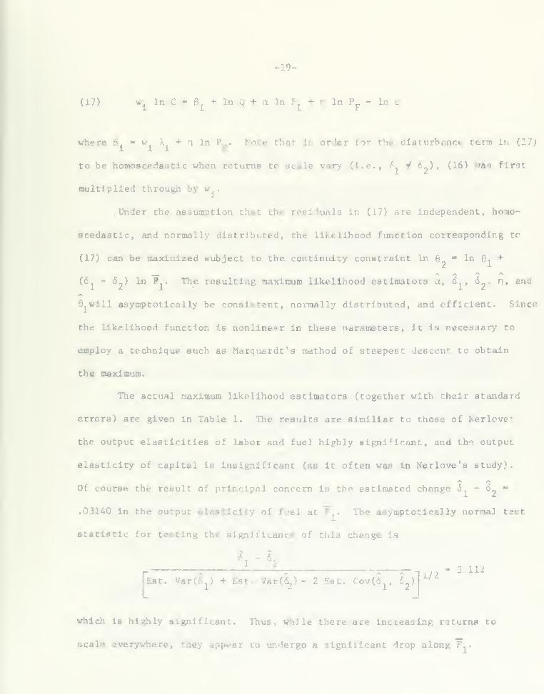
w. In. C - 6, + In a Pf+ n In Pr - In e
+ H In P^. Note that isturbancc term in
to be homoscedaatic when returns to scale vary (i.e., <*>.. i 6?), (16)
multiplied through by w .
ier the assumption that the residuals in (17) are independent, homo-
scedastic, and normally dit,r ed, the likelihood function corresponding
(17) can be maximized subject to the continuity constraint In 6- " In 0. +
(6. - 6„) In P . The resulting maximum likelihood estimators a, d. , 6?
, n» ana
.ill asymptotically be consistent, normally distributed, and efficient. Since
the likelihood function is nonlinear in these parameters, it is necessary to
employ a technique such as Marquardt's method of steepest descent to obtain
the maximum.
The actual maximum likelihood estimators (together with their standard
errors) are given in Table 1. The results are similiar to those of Nerlcve*
the output elasticities of labor and fuel highly significant, and the output
elasticity of capital is insignificant (as it often was in Nerlove's study).
Of course the result of principal concern is the estimated change 6. - 6~ m
.03140 in the on lastieity o! at F . The asymptotically normal testi.
statistic for testing the significance of this change is
112
(Est. Var ...-•.-
which is highly significant. Thu^ .e there are increasing raturns to
veryvhere, they appear to undergo a significant drop along F .


[I] Co! :ion, -i&
Supp.1. (1928), 139-165.
[2] Fu Jayne red Polynomials as Approximating Functions,"Australian Journal rlcultural Econon^ [ (June, 1969),35-46.
[3] Gallant, A. R. and Fuller, Wayne A., "Fitting Segmented PolynomialRegression Models Whose Join Points Have to be Estimate imalof the American Statistical Association , LXVIII (March, 1973), 144-147,
[4] Greene, William H. , "Factor Substitutions and Returns to Scale in
Electrical Supply," unpublished manuscript, 1974.
[5] Halpern, Elkan F. , "Bayesian Spline Regression when the Number of
Knots is Unknown," Journal of the Royal Statistical Society ,
(1973), 347-360.
[6] Hinkley, David V., "Inference in Two-Phase Regressirn," Journal ..;
the American Statistical Association , LXVI (December, 1971), 736-743.
[7] Horner, David, "The Impact of Negative Taxes on the Labor SupplyLow- Income Male Family Heads," in Final Report of the New JerseyGraduated Work Incentive Experiment (Madison: Institute forResearch on Poverty, University of Wisconsin, 1973), Chapter B-II
dson, Derek J., "Fitting Segmented Curves Wh 'n Points Haveto Be Estimated," Journal of the American Statistical Association ,
I (December, 1966), 1097-11.
[9] inMeasuremen t In St. (Stanford:Stanford Dnlvex 1963) ,
[10] Poirier, Dale J na in Economicsted dissertatio isconw 9
(II] , ewiee Regres sing Cubic SplinebJournal of the Amer^ atibtlcal Association , LXVIII (Septemb
1973), 5J
[12] , "On the Use of Bilinear Splinesming.


of Hu: