NASA/CR-97-206251

ICASE Report No. 97-64

th

,NNIVERSARY

On the Universality of the Kolmogorov Constantin Numerical Simulations of Turbulence

P. K. Yeung

Georgia Institute of Technology

Ye Zhou

ICASE and IBM

Institute for Computer Applications in Science and Engineering

NASA Langley Research Center

Hampton, VA

Operated by Universities Space Research Association

National Aeronautics and

Space Administration

Langley Research Center

Hampton, Virginia 23681-2199

Prepared for Langley Research Centerunder Contract NAS 1-19480

November 1997

https://ntrs.nasa.gov/search.jsp?R=19990004129 2018-07-11T02:03:55+00:00Z

Available from the following:

NASA Center for AeroSpace Information (CASI)800 Elkridge Landing Road

Linthicum Heights, MD 21090-2934

(301) 621-0390

National Technical Information Service (NTIS)

5285 Port Royal Road

Springfield, VA 22161-2171

(703) 487-4650

ON THE UNIVERSALITY OF THE KOLMOGOROV CONSTANT IN NUMERICAL

SIMULATIONS OF TURBULENCE*

P.K.YEUNG? AND YE ZHOU :_

Abstract. Motivated by a recent survey of experimental data [K.R. Sreenivasan, Phys. Fluids 7,

2778 (1995)], we examine data on the Kolmogorov spectrum constant in numerical simulations of isotropic

turbulence, using results both from previous studies and from new direct numerical simulations over a range

of Reynolds numbers (up to 240 on the Taylor scale) at grid resolutions up to 5123 . It is noted that

in addition to k -5/3 scaling, identification of a true inertial range requires spectral isotropy in the same

wavenumber range. We found that a plateau in the compensated three-dimensional energy spectrum at

k_? _ 0.1 - -0.2, commonly used to infer the Kolmogorov constant from the compensated three-dimensional

energy spectrum, actually does not represent proper inertial range behavior. Rather, a proper, if still

approximate, inertial range emerges at k_ ,_ 0.02 - 0.05 when R_ increases beyond 140. The new simulations

indicate proportionality constants C1 and C in the one- and three-dimensional energy spectra respectively

about 0.60 and 1.62. If the turbulence were perfectly isotropic then use of isotropy relations in wavenumber

space (C1 -- 18/55 C) would imply that C1 _ 0.53 for C -- 1.62, in excellent agreement with experiments.

However the one- and three-dimensional estimates are not fully consistcnt, because of departures (due to

numerical and statistical limitations) from isotropy of the computed spectra at low wavenumbers. The

inertial scaling of structure functions in physical space is briefly addressed. Since DNS is still restricted to

moderate Reynolds numbers, an accurate evaluation of the Kolmogorov constant is very difficult. We focus

on providing new insights on the interpretation of Kolmogorov 1941 similarity in the DNS literature and do

not consider issues pertaining to the refined similarity hypotheses of Kolmogorov (K62).

Key words. Kolmogorov constant, energy spectrum, numerical simulations

Subject classification. Fluid Mechanics

1. Introduction. Inertial-range behavior as postulated by Kolmogorov's (K41) similarity hypotheses

[1] is widely regarded as a fundamental characteristic of turbulence at high Reynolds number. In particular, in

the inertial range of intermediate scales the K41 result for the one-dimensional longitudinal energy spectrum

is given by

(1) Ell(k1) _- C1(e)2/3kl 5/3 ,

where kl is the longitudinal wavenumber, C1 is known as the Kolmogorov constant, and (e) is the mean

dissipation rate. Although K41 theory is subject to intermittency corrections associated with dissipation rate

fluctuations, such effects arc primarily manifested in higher-order statistics. Indeed, intermittency effects on

the second-order energy spectrum exponent are believed to be small and hardly measurable (Kolmogorov

[2], Frisch [3]), while at the same time may contribute to a persistence Reynolds number dependence for

higher-order structure functions (L'vov & Procaccia [4]).

*This research was supported in part by NSF Grant No. CTS-930 7973 to the first author, and by NASA under Contract

No. NAS1-19480 while the second author was in residence at ICASE.

tSchool of Aerospace Engineering, Georgia Institute of Technology, Atlanta, GA 30332.

Institute for Computer Applications in Science and Engineering, NASA Langley Research Center, Hampton, VA 23681

and IBM Research Division, T.J. Watson Research Center, P.O. Box, 218, Yorktown Heights, NY 10598.

The classical view of the "five-thirds" scaling law above, with substantial experimental support (e.g.,

Monin & Yaglom [5], Sec. 23.3), is that C1 has an universal value at asymptotically high Reynolds number.

Recently, however, there is renewed debate on the universality of C1, in part because of new measurements

at high Reynolds number (Praskovsky & Oncley [6]) and a subsequent new similarity theory (Barenblatt &

Goldenfeld [7]) that suggested a persistent Reynolds number dependence even at high Reynolds numbers.

On the other hand, the conclusion from a new and very extensive survey of experimental data by Sreeni-

vasan [8] is that, taken collectively, measurements do not support such a dependence for the Kolmogorov

constant. Sreenivasan found that the value of C1 averaged over the many different experiments cited is about

0.53 =i=0.055, although some corrections for the estimation of dissipation using local isotropy assumptions in

experiments may be warranted. It is still possible (Barenblatt & Goldenfeld [7], Sreenivasan [8]), though,

thatcontrolled experiments for a single geometry over a wide range of Reynolds numbers may reveal signifi-

cant trends otherwise masked by experimental scatter; new measurements of this nature (suggesting strong

Reynolds number dependence) have been reported by Mydiarski & Warhaft [9].

This paper is motivated by the survey of experimental data noted above, and will focus on similar

issues arising in numerical simulations of isotropic turbulence. We first review the basis for estimating the

Kolmogorov constant from previous studies, and then present new results from direct numerical simulations

(DNS) over a range of Reynolds numbers. Because of Reynolds number considerations, an accurate evaluation

of the Kolmogorov constant by DNS is admittedly very difficult. As such, we limit ourselves to the task of

providing new insights on the interpretation of K41 similarity in the DNS literature. For similar reasons,

we shall not consider the use of DNS to study issues pertaining to the refined similarity hypotheses of

Kolmogorov (K62) [2] (see, e.g., Chen et al. [10], Wang et al. [11] and others).

In numerical simulations, K41 similarity is frequently discussed in terms of the three-dimensional energy

spectrum function E(k) (where k is the wavenumber magnitude). If the turbulence at scale size 1/k is

isotropic then a kinematic constraint relating one- and three-dimensional spectra is

2 dk

Substitution of Eq. 1 into Eq. 2 implies that in the inertial range

(3) E(k) -- C<e>2/3k -5/3 ,

where C --- 55/18 C1. In principle, therefore, one may obtain either C or C1 (from three- and one-dimensional

spectra respectively) and infer the other using isotropy relations. Values of the Kolmogorov constant C

(estimated using either of these approaches) cited in a number of recent high resolution numerical studies

by other authors [11-21] are collected in Table I. Some relevant results from large-eddy simulations (LES)

are included also. (Note that we have quoted values of C from the highest-resolution data in each of these

references, since from the viewpoint of present paper we should not infer the Kolmogorov constant from

low-resolution simulations, especially in the older data.)

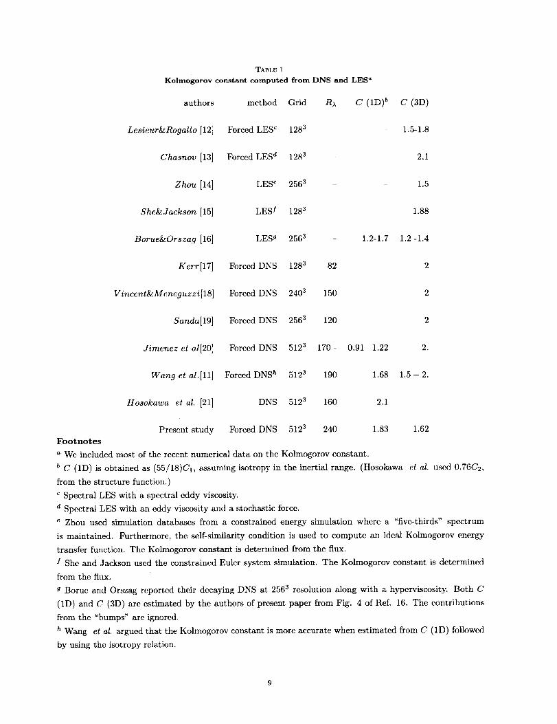
It may be noticed that most of the values displayed in Table I are higher than the value 1.619, which is

55/18 of the experimental average of 0.53 for C1. Note that, however, Zhou [14] found that the Kolmogorov

constant C = 1.5 from calculations of the spectra energy flux based on the self-similarity condition of the

triadic energy transfer hmction, in the form T(k, p, q) = a3T(ak, ap, aq) (where a is a scaling constant). A

commonly used procedure (e.g. Kerr [17], Jim_nez et al. [20]) for estimating the value of C is to plot the

"compensated" three-dimensional energy spectrum

(4) ¢(k) - E(k){e>-2/3k 5/3

asafunctionof wavenumbernormalizedbytheKolmogorovscale(r/),andto interpretC as the height of a

"plateau". However, it should be noted that whereas a flat region in the compensated spectrum implies k -5/3

behavior, the observation of a k -5/3 scaling range is not by itself a sufficient condition for an inertial range.

It is important that isotropy also be attained in the wavenumber range which displays k -5/3 behavior. (If

the isotropy requirement were relaxed then in principle one would have a different value of the "Kolmogorov

constant" in each direction, and the concept of universality would be lost.) Indeed, as will be seen in the

rest of this paper, our new results demonstrate that deviations from isotropy can contribute to values of C

that appear to be too high.

The major limitation in using DNS to examine inertial-range dynamics is, of course, the difficulty in

attaining high Reynolds numbers. However, recent advances in massively parallel computing have shown

significant promise. Our simulations were performed using a parallel implementation [22] of the well-known

Fourier pseudo-spectral algorithm of Rogallo [23] on the IBM SP at the Corncll Theory Center. The highest

grid resolution used is 5123, with a Taylor-scale Reynolds number (Rx) about 240 averaged over about

four eddy-turnover times. Whereas this Reynolds number is not high compared to some recent laboratory

experiments (Rx 473 in Mydlarski & Warhaft [9]), it is about the same as (or slightly higher than) the

highest values reported in the DNS literature (for example, Rx 218 in Cao et al. [24]). Numerical results

on spectra as well as structure functions (to which Kolmogorov [1] originally referred) are given in the next

section. In order to characterize issues of Reynolds number dependence and attempt to quantify a minimum

Reynolds number threshold above which inertial-range behavior could bc expected, we present data at five

different grid resolutions.

To maintain a stationary state so that results may be averaged over time at the highest Reynolds number

possible using a given number of grid points, it is usual to apply numerical forcing at the large scales. In the

literature this has been done in several different ways, such as adding a stochastic forcing term (Eswaran

& Pope [25]), holding the energy in the lowest-wavenumber shells fixed while allowing phase information

to evolve (Chen et al. [10], Sullivan et al. [26]), or by introducing a negative viscosity in these shells

(Jim6nez et al. [20]). Alternatively, LES [12-15], with and without forcing, as well as simulations with a

hyperviscosity [16] can also be used to achieve higher Reynolds numbers. However, it is generally believed

that (e.g., see Rcf. 20), the precise manner of forcing provided it is applied to the largest scales in the

flow-has no systematic effects on the inertial-range energy spectrum, nor on the statistical character of

the small scales. Whereas in this work we have used the scheme of Eswaran & Pope [25], we have checked

that similar calculations in which the energy in the first couple of wavenumber shells is fixed do not warrant

different conclusions.

2. Results. We present spectra and structure functions from simulations of forced stationary isotropic

turbulence averaged over relatively long time periods. Major simulation parameters are summarized in

Table II. For the less expensive 643 and 1283 runs the averaging time (T) shown is the aggregate of multiple

simulations of shorter duration. In all cases the small scales are considered to be well resolved, as measured

by kmax_ _ 1.5, where kma_ is the highest wavenumber represented by the grid points. The non-dimensional

quantity (e)L1/u '3 (where L1 is the longitudinal integral length scale derived from the longitudinal velocity

correlation, and u t is the r.m.s, velocity) in the last column of this table is of interest in the scaling of (e)

with ul3/L1 using energy cascade arguments; it appears to approach a constant at high Reynolds numbers.

This trend is similar to that found in the simulations of Jim6nez et al. [20], Wang et al. [11] and Cao et

al. [24], and to that in experiments (Sreenivasan [27], Fig. 1). The differences among different "asymptotic"

numerical values are due in part to differences in the definition of integral scales and in flow conditions in

experimentsandnumericalsimulations.

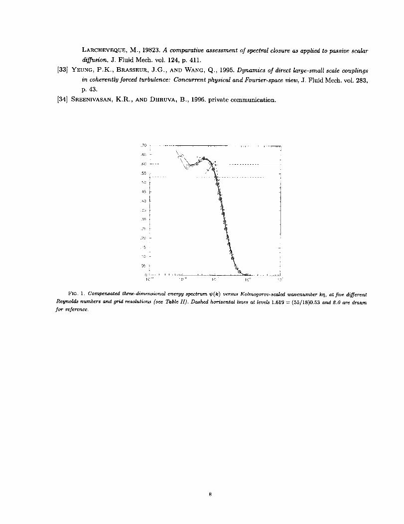
Figure1 showsthe three-dimensionalcompensatedspectrum_b(k)in Kolmogorovscaling.(Note:intheseandall otherfigureslinesA - E refer to data at five different grid resolutions from 643 to 5123

respectively, as listed in Table II.) Except for small spectral turn-ups at the high wavenumber end resulting

from residual aliasing errors, small-scale universality is unambiguously achieved, even at the lowest Reynolds

number (R_ 38 in 643 simulations). Two relatively flat (i.e. k -5/3) regimes of limited extent can be seen:

namely at k_? _-, 0.1 - 0.2 in the form of a bumpy "plateau" which is seen at all grid resolutions, and in the

low-wavenumber range k_ _ 0.02 - 0.05 which is captured only at higher (2563 and beyond) resolutions.

If the former were taken to represent the inertial range then one would obtain a Kolmogorov constant C

greater than 2.0, as reported by a number of other authors (see Table I). On the other hand, it is clear that

the level of ¢(k) in the range k_? _, 0.02 - 0.05 agrees well with experimental data, if one uses the isotropy

relation C -- 55/18 C1, which would imply C1 -- 18/55 C _ 0.53. It is our objective in the analyses below

to establish that this lower-wavenumber region, rather than the plateau, represents (the beginnings of) a

proper inertial range.

In order that inertial range dynamics can be independent of both the large-scale energetics and viscous

dissipation, a wide scale separation must exist between the peaks of the energy and dissipation spectra in

wavenumber space. The peak of E(k) occurs in the lowest two wavenumber shells (k_/_, 0.01 for the 5123

data), whereas from a plot of the dissipation spectrum we find that the peak of D(k) =_ 2vk2E(k) occurs

at k_/_ 0.17. This location of the dissipation spectral peak is virtually the same as found by Wang et

al. [11]. Since this almost coincides with the "plateau" in Fig. 1 it is clear that the plateau should not be

taken as an indication of inertial-range behavior. In fact, this plateau may be identified with the so-called

"bottleneck" phenomenon that has been discussed in experimental (Saddoughi & Veeravalli [28]), theoretical

(Falkovich [29]), and numerical (Borue & Orszag [30]) work. According to this theory, viscous effects on

spectral transfer causes an increase (relative to k -5/3 in the energy spectrum at intermediate wavenumbers.

Nonlocal interactions among Fourier modes well separated in scale (Brasseur & Wei [31]) are also believed

to play an important role (Herring et al. [32]). We also note that Brasseur & Wei argued that there should

be about a decade in scale separation between the wavenumber where the inertial range "ends" and the

dissipation peak, which is more than that (about 3 to 4) found in DNS (Wang et al. [11] and this paper).

A full understanding of this latter issue awaits future high-resolution simulations and experimental data.

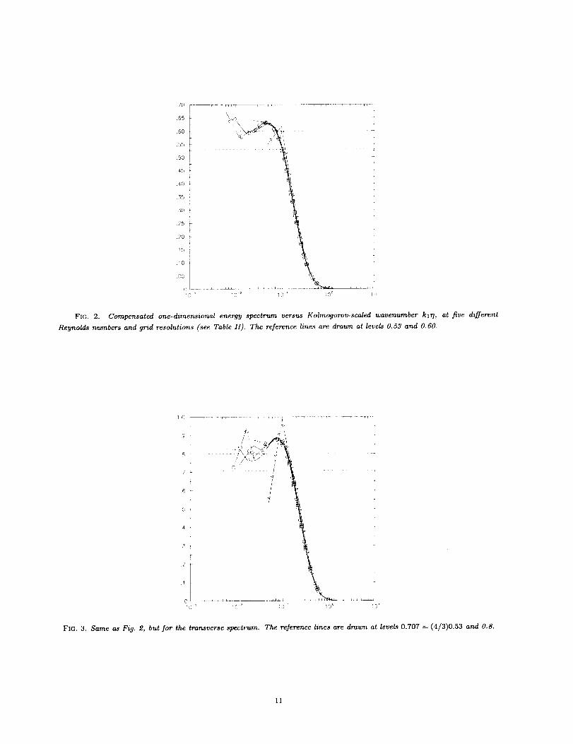
A more direct comparison with experiment may be made by considering the compensated longitudinal

energy spectrum, i.e. _)1 (kl) : Ell (kl)(e>-2/3k5/3, which is shown in Fig. 2. Because this spectrum drops

off very rapidly at high wavenumbers, we have used log-linear scales to highlight the function values at any

wavenumber ranges where ¢1 is approximately constant. Two such ranges can be seen, corresponding to

those for ¢ but in each case occurring at lower wavenumbers. The observation that the peak of ¢1(kl)

occurs at kl y ----0.05 is similar to high Reynolds number measurements in both boundary layers (Saddoughi

& Veeravalli [28]) and grid turbulence (Mydlarski & Warhaft [9]). It is also apparent that the value of

C1 inferred from this figure is about 0.60, which is somewhat higher than, but still relatively close to the

experimental average [5] of 0.53.

From Figs. 1 and 2 we may conclude that the best values obtained for C1 from the three- and one-

dimensional spectra are about 0.53 and 0.60 respectively. These values (especially the former) are closer to

experiment than those cited previously in the literature. Yet there is evidently some inconsistency between

these two estimates for C1. These differences are due to deviations from isotropy in wavenumber space, as

further studied below.

In additionto Ell(kl) we have also computed the transverse energy spectrum, for which the classical

inertial-range result is

(5)

where isotropy requires C_ = _C1.

E22 (kl) = C_ (_) 2/3 k15/3 ,

The compensated transverse spectrum (Fig. 3) exhibits a similar but

stronger bump at kl_/ _ 0.07. We also find that the ratio E22(k1)/E11(kl) is close to 4/3 in the range

kl_/_ 0.02 - 0.04, but increases steadily with wavenumber beyond this range.

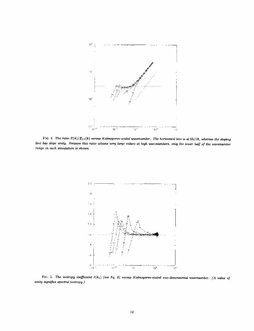
If a five-thirds scaling holds for both one- and three-dimensional spectra over the same wavenumber

range then the hmctions E(k) and Ell(k) should be proportional within this range. Figure 4 shows the

spectral ratio E(k)/En(k), compared with the classical inertial range value of 55/18. It may be seen that,

at the wavenumber range (k_? _ 0.1 - 0.2) corresponding to the plateau in Fig. 1, this ratio is considerably

higher than 55/18 and in fact increases roughly in proportion to k_/. This observation provides further

evidence that the plateau in ¢ does not represent an inertial range. The transition from behavior without

a level region to one at a value close to 55/18 (at Rx 240 at 5123 resolution) occurs between R_ 90 (on an

1283 grid) and R_ 140 (for 2563). The ratio C/C1 inferred in this manner is seen to be somewhat less than

55/lS.It should be noted that isotropy of the spectral tensor is a key requirement for the relation C = 55/18C1.

Although the simulations arc of (nominally) isotropic turbulence, departures of the computed spectra from

isotropy are, in fact, not totally unexpected. It is well-known that sampling hmitations arise in the lowest

few wavenumber shells because relatively few samples of the large scales are present in a solution domain

of finite size. _rthermore, since the solution domain in physical space is a cube (rather than a sphere),

the averaged statistics are at best invariant among the three Cartesian coordinate axes, but do not satisfy

the stricter requirement of no preferential orientation in three-dimensional space. As an example we may

note that whereas the periodicity length of the flow along the coordinate axes is equal to the length of each

side of the solution domain, it is longer if measured along directions inclined to the axes. This effect is felt

primarily in spatial correlations over large separations in space, which correspond to low wavenumbers in

Fourier space.

In Figs. 6 and 7 these structure functions are shown in Kolmogorov scaling in order to compare with

the theoretical proportionality constants C2 _ 4.02 C1 and -4/5. It is clear that the highest Reynolds

number data shown agree well with classical inertial range results. Numerical values of --DLLL(r)/<C)r at

intermediate resolutions also fit in well within the Reynolds number trend suggested by new measurements

in grid turbulence over a range of Reynolds numbers (Sreenivasan & Dhruva [35]).

It is perhaps worth noting that the highest-resolution (5123) simulation reported is at a higher Reynolds

number and are averaged over a greater number of large-eddy turnover times than several other studies

reporting 5123 results (e.g., Jim6nez et al. [20], Chen et al. [10], Wang et al. [11]) for stationary

isotropic turbulence. The spectra and structure functions obtained from these and the present simulations

demonstrate that, with the latest advances in massively parallel computing, issues concerning inertial-range

similarity in DNS can now be addressed in a more reliable manner than possible before.

3. Conclusions . We have presented new results on the Kolmogorov scaling of energy spectra and

structure hmctions in the inertial range, from direct numerical simulations of stationary isotropic turbulence

ranging from R_ 38 (on a 643 grid) to R_ 240 (on 5123). It is pointed out that a plateau in the compen-

sated three-dimensional energy spectrum at kT/_ 0.1-0.2 commonly used to infer the Kolmogorov constant

from the compensated three-dimensional energy spectrum in fact does not represent proper inertial range

behavior.Instead,a proper(if still approximate)inertialrangeemergesat k_ _ 0.02 - 0.05 when R_ in-

creases beyond 140. We find that the proportionality constants C and C1 in the three- and one-dimensional

compensated energy spectra are about 1.62 and 0.60 respectively. These values are closer to experimental

data than reported in most previous numerical simulations. In particular, if isotropy relations are used then

we may infer from the three-dimensional spectra that C1 = 18/55 C _ 0.53, in excellent agreement with

experimental data (Sreenivasan [8]). However, the ratio C/C1 in our results differs from the theoretical value

of 55/18, because of significant departures from isotropy in the computed spectra at the wavenumber range

where inertial-range behavior is otherwise reasonably well approximated. Results on second- and third-order

structure functions over a range of Reynolds numbers further suggest that the simulation database that we

have accumulated should be useful for investigating other aspects of similarity scaling and Reynolds number

dependence.

We emphasize that a k -5/3 scaling is in itself not a sufficient indicator of inertial-range behavior. To

achieve a strictly isotropic inertial range in direct numerical simulations requires that the inertial scales be

small compared to the size of the solution domain. Whereas it is difficult to meet this requirement well, it

seems clear that high-resolution simulations using the techniques of massively parallel computing are very

helpful.

Acknowledgments. We are grateful to Professor K.R. Sreenivasan for many stimulating discussions

and his constant encouragement, as well as comments on an early draft of this paper. In addition we thank

Professors Jim Brasseur, Zellman Warhaft, Drs. Shiyi Chen and Jack Herring for their valuable input.

Figures 6 and 7 evolved from joint work between the first author and Dr. Michael Borgas, within NSF Grant

INT-9526868. The computations were performed using the supercomputing resources of the Cornell Theory

Center, which receives major funding from NSF and New York State.

REFERENCES

[1] KOLMOGOROV, A.N., 1941. The local structure of turbulence in incompressible viscous fluids for very

large Reynolds numbers, Dokl. Akad. Nauk SSSR, vol 30, p. 301.

[2] KOLMOGOROV, A.N., 1962. 'A refinement of previous hypotheses concerning the local structure of tur-

bulence in a viscous incompressible fluid at high Reynolds number, J. Fluid Mech. vol. 13, p. 82.

[3] FRISCH, U., 1995. Turbulence: The Legacy of A.N. Kolmogorov, Cambridge University Press.

[4] L'VOV, V.S., AND PROCACCIA, I., 1995. Intermittency in hydrodynamic turbulence as intermediate

asymptotics to Kolmogorov scaling, Phys. Rev. Lett. vol. 74, p. 2690.

[5] MONIN, A.S, AND YAGLOM, A.M., 1975. Statistical Fluid Mechanics, Vol. II, MIT Press.

[6] PRASKOVSKY, A., AND ONCLEY, S., 1994. Measurements of the Kolmogorov constant and intermittency

exponent at very high Reynolds numbers, Phys. Fluids, vol. 6, 2886.

[7] BARENBLATT, G.I., AND GOLDENFELD, N., 1995. Does fully developed turbulence exist? Reynolds

number independence versus asymptotic covariance, Phys. Fluids, vol. 7, 3078. bitem

[8] SREENIVASAN, K.R., 1995. On the universality of the Kolmogorov constant, Phys. Fluids, p. 2778.

[9] MYDLARSKI, L., AND WARHAFT, Z., On the onset of high-Reynolds-number grid-generated wind tunnel

turbulence, J. Fluid Mech., vol. 320, 331.

[10] CHEN, S., DOOLEN, G.D., KRAICHNAN, R.H., AND SHE, Z.-S., 1993. On statistical correlations

between velocity increments and locally averaged dissipation in homogeneous turbulence, Phys. Fluids

A, vol. 5, 458.

[11] WANG, L.P., CHEN, S., BRASSEUR, J.G., AND WYNGAARD, J.C., 1996. Examination of hypotheses

in the Kolmogorov refined turbulence theory through high-resolution simulations: Part 1. Velocity

field, J. Fluid Mech., vol. 309, 113.

[12] LESIEUR, M. & ROGALLO, R.S., 1989. Large-eddy simulation of passive scalar diffusion in isotropic

turbulence, Phys. Fluids A, vol. 1, p.718.

[13] CHASNOV, J.R., 1991. Simulation of the Kolmogorov inertial range using an improved subgrid model,

Phys. Fluids A, vol. 1, p.945.

[14] ZHOU, Y., 1993. Interacting scales and energy transfer in isotropic turbulence, Phys. Fluids A, vol. 5,

p.2524.

[15] SHE, Z.-S., AND JACKSON, E., 1993. A constrained Euler system for Navier-Stokes turbulence, Phys.

Rev. Lett., vol. 70, 1255.

[16] BORUE, V., AND ORSZAG, S.A., 1995. Self-similar decay of three-dimensional homogeneous turbulence

with hyperviscosity, Phys. Rev. E, vol. 51, p. R856.

[17] KERR, R.M., 1990. Velocity, scalar, and transfer spectra in numerical turbulence J. Fluid Mech., vol.

211, p.309.

[18] VINCENT, A., AND MENEGUZZI, M., 1991. The spatial structure and statistical properties of homoge-

neous turbulence, J. Fluid Mech., vol. 225, p. 1.

[19] SANADA, T., 1992. Comment on the dissipation-range spectrum in turbulent flows, Phys. Fluids A, vol.

4, p. 1086.

[20] JIMI_NEZ, J., WRAY, A.A., SAFFMAN, P.G., AND ROGALLO, R.S., 1993. The structure of intense

vorticity in isotropic turbulence, J. Fluid Mech., vol. 255, 65.

[21] HOSOKAWA, I., OIDE, S., AND YAMAMOTO, K., 1996. Isotropic turbulence: important differences

between true dissipation rate and its one-dimensional surrogate, Phys. Rev. Lctt., vol. 77, 4548..

[22] YEUNG, P.K., AND MOSELEY, C., 1995. in Parallel Computational Fluid Dynamics: Implementations

and Results Using Parallel Computers., eds. A. Ecer, J. Pcriaux, N. Satofuka _ S. Taylor (Elsevier,

Amsterdam), 473.

[23] ROGALLO, R.S., 1981. Numerical experiments in homogeneous turbulence, NASA Tcch. Memo. 81315.

[24] CAO, N., CHEN, S., AND DOOLEN, G., 1996. Statistics and structure of pressure in isotropic turbu-

lence", Submitted to Phys. Fluids.

[25] ESWARAN, V., AND POPE, S.B., An examination of forcing in direct numerical simulations of turbu-

lence, Comput. & Fluids, vol. 16, p. 257.

[26] SULLIVAN, N.P., MAHALINGHAM, S., AND KERR, R.M., 1994. Deterministic forcing of homogeneous,

isotropic turbulence, Phys. Fluids vol. 6, 1612.

[27] SREENIVASAN, K.R., 1984. On the scaling of the turbulence energy dissipation rate, Phys. Fluids vol.

27, p.1048.

[28] SADDOUGHI, E.G., AND VEERAVALLI, S.V., 1994. Local isotropy in turbulent boundary layers at high

Reynolds number, J. Fluid Mech., vol. 268, p. 333.

[29] FALKOVICH, G., 1994. Bottleneck phenomenon in developed turbulence, Phys. Fluids vol. 6, p. 1411.

[30] BORUE, V., AND ORSZAG, S.A., 1996. Numerical study of three-dimensional Kolmogorov flow at high

Reynolds numbers, J. Fluid Mech. vol. 306, p. 293.

[31] BRASSEUR, J.G., AND WEI, C.H., 1994. Interscale dynamics and local isotropy in high Reynolds

number turbulence within triadic interactions, Phys. Fluids vol. 6, p. 842.

[32] HERRING, J.R., SCHERTZER, D., LESIEUR, M., NEWMAN, G.R., CHOLLET, J.P., AND

LARCHEVEQUE,M., 19823.A comparative assessment of spectral closure as applied to passive scalar

diffusion, J. Fluid Mech. vol. 124, p. 411.

[33] YEUNG, P.K., BRASSEUR, J.G., AND WANG, Q., 1995. Dynamics of direct large-smaU scale couplings

in coherently forced turbulence: Concurrent physical and Fourier-space view, J. Fluid Mech. vol. 283,

p. 43.

[34] SREENIVASAN, K.R., AND DHRUVA, B., 1996. private communication.

.60

.55

50

45

40

3b

50

25

.20

Ib

10

O5

00_; --_

FIG. 1. Compensated three-dimensional energy spectrum lp(k) versus Kolmogorov-scaled wavenumber ko, at five different

Reynolds numbers and grid resolutions (see Table 11}. Dashed horizontal lines at levels 1.619 = (55/18)0.53 and _.0 are drawn

for reference.

Footnotes

TABLE 1

Kolmogorov constant computed from DNS and LES a

authors

Lesieur&Rogallo [12]

Chasnov [13]

Zhou [14]

She&Jackson [15]

Borue&Orszag [16]

Kerr[17]

V incent_ M eneguz zi [18]

Sanda[19]

Jimenez et a/[20]

method Grid R_ C (1D) b

Forced LESc 1283

C (3D)

1.5-1.8

a We included most of the recent numerical data on the Kolmogorov constant.

Wang et a/.[11] Forced DNS h 5123 190 1.68 1.5- 2.

Hosokawa et al. [21] DNS 5123 160 2.1

Present study Forced DNS 5123 240 1.83 1.62

LES _ 2563 1.5

LES f 1283 1.88

LES 9 2563 1.2-1.7 1.2 -1.4

Forced DNS 1283 82 2

Forced DNS 2403 150 2

Forced DNS 2563 120 2

Forced DNS 5123 170 - 0.91 1.22 2.

b C (1D) is obtained as (55/18)C,, assuming isotropy in the inertial range. (Hosokawa et al. used 0.76C2,

from the structure function.)

Spectral LES with a spectral eddy viscosity.

d Spectral LES with an eddy viscosity and a stochastic force.

Zhou used simulation databases from a constrained energy simulation where a "five-thirds" spectrum

is maintained. _rthermore, the self-similarity condition is used to compute an ideal Kolmogorov energy

transfer function. The Kolmogorov constant is determined from the flux.

f She and Jackson used the constrained Euler system simulation. The Kolmogorov constant is determined

from the flux.

g Borue and Orszag reported their decaying DNS at 2563 resolution along with a hyperviscosity. Both C

(1D) and C (3D) are estimated by the authors of present paper from Fig. 4 of Ref. 16. The contributions

from the "bumps" are ignored.

h Wang et al. argued that the Kolmogorov constant is more accurate when estimated from C (1D) followed

by using the isotropy relation.

Forced LES d 1283 2.1

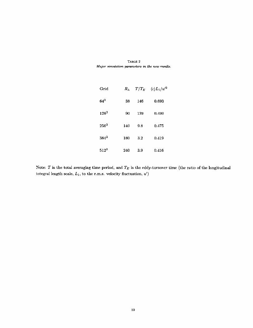
TABLE 2

Major simula$ion parameter8 in the new results.

Grid R_ T/TE (e)L_/u '3

643 38 146 0.693

1283 90 139 0.499

2563 140 9.8 0.475

3843 180 3.2 0.419

5123 240 3.9 0.416

Note: T is the total averaging time period, and TE is the eddy-turnover time (the ratio of the longitudinal

integral length scale, L1, to the r.m.s, velocity fluctuation, u _)

10

70

65

60

55

50

45

40

_5

_0

25

20

!5

"0

05

0

_r_ T r_

1,9 _ 1,3 '

L

i ©_ 10'

FIG. 2. Compensated one-dimensional eneryy spectrum versus Kolmogorov-scaled wavenumber k171, at five different

Reynolds numbers and grid resolutions (see Table II). The reference lines are drawn at levels 0.53 and 0.60.

FIG. 3. Same as Fig. 2, but for the transverse spectrum. The reference lines are drawn at levels 0.707 = (4/3)0.53 and 0.8.

11

10 2

10'

10 °

! j "! ' / ' ,/':f

10 I . ___ ____.1,1_ J , i ,,i,,i

10 -_ !0 -_ 10-' 10 _' 10'

FIG. 4. The ratio E(k)/Ell (k) versus Kolmogorov-scaled wavenumber. The horizontal line is at 55/18, whereas the sloping

line has slope unity. Because this ratio attains very large values at high wavenumbers, only the lower half of the wavenumber

range in each simulation is shown.

1E

16

1.4

12

10

6

4

10 _

,/ tO ' :

l 4_: i "r10 _ 10-' 10 ° 10'

Fro. 5. The isotropy coefficient l(kl) (see Eq. 6) versus Kolmogorov-sealed one-dimensional wavenumber. (A value of

unity signifies spectral isotropy.)

12

10 :'

+[, ;I

1C + !C,' 10; 1('_,_

FIG. 6. Kolmogorov scaling of the second-order longitudinal structure .function versus r/eta. The horizontal line is at

2.13 = (4.02)(0.53); the sloping dashed line indicates universal behavior of the small scales, as (1/15)(r/_l)a/3 .

10 c

10'

10 +

+,#" '\ + ,, +'+

] _ + I+;/ i

lC G 1O' 10 a 10 _

FIG. 7. Kolmogorov scaling of the third order longitudinal structure function versus r/eta. The horizontal line is at O.8.

13

REPORT DOCUMENTATION PAGE Fo_mApprovedOMB No. 0704-0188

Pubticreportingburdenfor this collectionof informationisestimatedto average1 hourperresponse,includingthe time Forreviewinginstructions,searchingexistingdatasources,pthering and maintainingthe data needed,andcompletingandreviewing the collectionof information Send commentsregardingthisburdenestimateor any otheraspectof thiscollectionOFinfocmation, includingsuKKestionsfor reducing thisburden,to WashingtonHeadquartersServices,Directoratefor InformationOperationsand Reports, 1215JefTersonDavisHighway,Suite 1204, Arlington,VA 22202-4302,and to the Officeof Managementand Budget,PaperworkReductionProject(0704-0188l, Washington,DC 20503.

1. AGENCY USE ONLY(Leave blank) 2. REPORT DATE 3. REPORT TYPE AND DATES COVERED

November 1997 Contractor Report

4. TITLE AND SUBTITLE 5, FUNDING NUMBERS

On the Universality of the Kolmogorov Constant in Numerical Sim-

ulations of Turbulence

6. AUTHOR(S)

P.K. Yeung

Ye Zhou

7. PERFORMING ORGANIZATION NAME(S) AND ADDRESS(ES)

Institute for Computer Applications in Science and Engineering

Mail Stop 403, NASA Langley Research Center

Hampton, VA 23681-0001

9. SPONSORING/MONITORING AGENCY NAME(S) AND ADDRESS(ES)

National Aeronautics and Space Administration

Langley Research Center

Hampton, VA 23681-2199

C NAS1-19480

WU 505-90-52-01

8. PERFORMING ORGANIZATIONREPORT NUMBER

ICASE Report No. 97-64

10. SPONSORING/MONITORINGAGENCY REPORT NUMBER

NASA CR-97-206251

ICASE Report No. 97-64

11. SUPPLEMENTARY NOTES

Langley Technical Monitor: Dennis M. Bushnell

Final Report

Submitted to Physical Review E

12a. DISTRIBUTION/AVAILABILITY STATEMENT 12b. DISTRIBUTION CODE

Unclassified-Unlimited

Subject Category 34

Distribution: Nonstandard

Availability: NASA-CASI (301)621-0390

13. ABSTRACT (Maximum 200 words)

Motivated by a recent survey of experimental data [K.R. Sreenivasan, Phys. Fluids 7, 2778 (1995)], we examine

data on the Kolmogorov spectrum constant in numerical simulations of isotropic turbulence, using results both from

previous studies and from new direct numerical simulations over a range of Reynolds numbers (up to 240 on the

Taylor scale) at grid resolutions up to 5123. It is noted that in addition to k -5/3 scaling, identification of a true

inertial range requires spectral isotropy in the same wavenumber range. We found that a plateau in the compensated

three-dimensional energy spectrum at kr/,_ 0.1 - -0.2, commonly used to infer the Kolmogorov constant from the

compensated three-dimensional energy spectrum, actually does not represent proper inertial range behavior. Rather,

a proper, if still approximate, inertial range emerges at kt/_ 0.02 - 0.05 when R_ increases beyond 140. The new

simulations indicate proportionality constants C1 and C in the one- and three-dimensional energy spectra respectively

about 0.60 and 1.62. If the turbulence were perfectly isotropic then use of isotropy relations in wavenumber space

(C1 = 18/55 C) would imply that C1 _ 0.53 for C = 1.62, in excellent agreement with experiments. However the

one- and three-dimensional estimates are not fully consistent, because of departures (due to numerical and statistical

limitations) from isotropy of the computed spectra at low wavenumbers. The inertial scaling of structure functions

in physical space is briefly addressed. Since DNS is still restricted to moderate Reynolds numbers, an accurate

evaluation of the Kolmogorov constant is very difficult. We focus on providing new insights on the interpretation

of Kolmogorov 1941 similarity in the DNS literature and do not consider issues pertaining to the refined similarity

hypotheses of Kolmogorov (K62).

14, SUBJECT TERMS

Kolmogorov constant, energy spectrum, numerical simulations

17. SECURITY CLASSIFICATIONOF REPORT

Unclassified

_SN 7540-01-280-5500

18. SECURITY CLASSIFICATION lg. SECURITY CLASSIFICATIOI_OF THIS PAGE OF ABSTRACT

Unclassified

15. NUMBER OF PAGES

18

16. PRICE CODE

A0320. LIMITATION

OF ABSTRACT

|

Standard Form 298(Rev. 2-89)Prescribed by ANSI Std. Z39-18

298-102