On The Transport Of Energy in Water Waves

Marshall P. Tulin

Professor Emeritus, UCSBmpt6@cox.net

Abstract

Theory is developed and utilized for the calculation of the separate transport of kinetic, gravitypotential, and surface tension energies within sinusoidal surface waves in water of arbitrary depth.

In Section 1 it is shown that each of these three types of energy constituting the wave travel atdifferent speeds, and that the group velocity, cg, is the energy weighted average of these speeds,depth and time averaged in the case of the kinetic energy. It is shown that the time averagedkinetic energy travels at every depth horizontally either with (deep water), or faster than the waveitself, and that the propagation of a sinusoidal wave is made possible by the vertical transport ofkinetic energy to the free surface, where it provides the oscillating balance in surface energy justnecessary to allow the propagation of the wave. The propagation speed along the surface of thegravity potential energy is null, while the surface tension energy travels forward along the wavesurface everywhere at twice the wave velocity, c.

The flux of kinetic energy when viewed traveling with a wave provides a pattern of steadyflux lines which originate and end on the free surface after making vertical excursions into thewave, even to the bottom, and these are calculated. The pictures produced in this way provideimmediate insight into the basic mechanisms of wave motion.

In Section 2 the modulated gravity wave is considered in deep water and the balance of termsinvolved in the propagation of the energy in the wave group is determined; it is shown again thatvertical transport of kinetic energy to the surface is fundamental in allowing the propagation ofthe modulation, and in determining the well known speed of the modulation envelope, cg.

Dedicated to Professor J.N. Newman in recollection of his many significant contributions to thetheory and computation of waves and floating bodies and to the founding of the IWWWFB.

Introduction

Energy transport in waves has in the past been almost inextricably interwoven with the conceptof wave ‘group velocity.’ The later arose from the very elemental observation of Scott Russell (1844),as quoted here in Lamb (1932, p.380): “It has often been noticed that when an isolated group ofwaves, of sensibly the same length, is advancing over relatively deep water, the velocity of the groupas a whole is less than that of the individual waves composing it. If attention be fixed on a particularwave, it is seen to advance through the group, gradually dying out as it approaches the front, whilstits former place in the group is occupied in succession by the waves which have come forward fromthe sea.”

The first explanation of the group phenomenon in terms of the dispersive character of waterwaves was kinematical in nature, Stokes (1876), soon generalized by Rayleigh (1877a; 1877b) to avariety of waves in fluids, as well as to flexural waves in beams. The kinematical result, derived fromsuperposition of two dispersive waves of infinitesimally differing wave length, is that the group velocityis precisely the derivative of the frequency, ω, with respect to wave number, k: cg = dω/dk.

The connection between the group velocity and energy flux was made by Osborne Reynolds (1877),who showed that the time averaged energy transported across any transverse plane in a train of deepwater linear waves is only half of the energy necessary to supply the waves which pass in the same

1

time, and this result was extended to water of arbitrary depth by Rayleigh (1877b, pg.479), who alsoin the same paper provided a derivation alternative to Reynold’s, and applicable to arbitrary waves.This derivation depended on the artifice of considering the wave number to have a small imaginarycomponent.

From this time (1877), and leaving aside questions which arise in the non-linear wave regime, thestate of affairs regarding energy transport in waves has remained essentially as left by Rayleigh; forevidence of this see the masterly pedagogical discussions in Sir James Lighthill’s (1978), “Theory ofWaves.”

The group velocity, subsequent to Rayleigh, made its appearance in the asymptotic analysis (sta-tionary phase) of water waves and its meaning and application were both extended to the treatmentof wave spectra, modulating waves, wave patterns (as the Kelvin ship wave), internal waves, andothers. In fact, its presence in wave theory is ubiquitous. There do remain questions however. Theunderlying connection between the separate kinematical and energy propagation origins of the groupvelocity remains obscure. Its meaning and definition in the non-linear regime of water waves offersdifficulties as well, see the discussion in Peregrine and Thomas (1979).

In the present paper we are concerned with more than the group velocity itself, particularly withsome very basic questions regarding the true nature of energy transport within the wave, and itsrelation to the mechanism of wave motion: (i) Do all components of the wave energy (kinetic, gravitypotential, and surface tension) travel at the group velocity, cg, uniform within the wave, and if not,how do they propagate? and (ii)What role do these transport speeds play in the mechanism of wavepropagation itself, both for the basic wave and for the modulation envelope?

The surprising answers to these questions, already indicated in the Abstract above, may be foundwithin the context of the linear sinusoidal wave, and its second order counterpart in the case ofmodulating waves. They allow us a more complete and satisfying physical understanding, in terms ofenergy transport, of the actual physical mechanism underlying the very existence of sinusoidal wavesand wave groups in general, including wave fronts.

It should be mentioned, for the sake of historical completeness, that the kinetic energy producedin the ideal fluid through the motion of a body was appreciated by 19th c. theorists as central in thetreatment of the body’s dynamics, and led to the concept of the added mass tensor for which formulaewere early produced, see Lamb (1932). Nevertheless, beyond the calculation of the total field kineticenergy, important fundamental questions remain to this day: How does the energy flow from themoving body, parts of which must be doing work on the fluid, and then penetrate into the fluid,permeating it and thus creating the flow field which connects through the fluid with the body? Then,in what way does the fluid return energy to the body in other parts, making possible the existence ofbody motion without resistance in a perfect fluid?

These questions, although beyond our present scope, can however be answered for planar bodiesusing certain fundamental relations introduced herein, as well as the device of energy flux lines.

1 General Theory

1.1 Flux in a continuous media

The temporal change of a scalar quantity lies in the balance between its generation and thegradients of its flux, and can therefore always be written:

∂e

∂t+ ∇ · ~Fe = Qe [1.1]

2

where ~Fe is the flux of e and Qe its “source,” each defined locally in space and time. When consideredwhile moving locally with the velocity ~vR,

de

dt=

∂e

∂t+ ~vR · ∇e = Qe −∇ · ~Fe + ~vR · ∇e

so that,de

dt+ ∇ · [~Fe − ~vRe] = Qe − e[∇ · ~vR] [1.2]

and the effective flux and source are thus seen to depend on observation.The flux defined through [1.1] and [1.2] quantifies the transport of the scalar and thereby defines

a transport velocity, ~ce,

~ce =~Fe

e− ~vR [1.3]

1.2 Kinetic energy flux in an ideal fluid

The transport of the kinetic energy density (ρq2/2 = ρ~u · ~u), within an irrotational (~u = ∇φ),incompressible (∇2φ = 0) flow is readily found. By definition,

KE =ρq2

2=

ρ

2∇ · (φ∇φ)

and taking into account incompressibility, a conservation law in the form of [1.1] results.

∂KE

∂t=

ρ

2∇ · {φt∇φ + φ∇φt}

=ρ

2{φt∇

2φ + φ∇2φt} + ρ{∇φt∇φ}

= ρ∇ · {φt∇φ}

or,∂KE

∂t−∇ · [ρφt~u] = 0 [1.4]

and therefore,~F (KE) = −ρφt~u; Q(KE) = 0 [1.5]

This, [1.5], is the Eulerian flux, which is seen to be in the direction of the particle velocity. Corre-spondingly, the Lagrangian flux is taken following a particle by setting ~vR = ~u in [1.2],

~F (KE; ~u) = −ρ~u

(φt +

q2

2

)[1.6]

1.3 KE Flux for a uniformly translating planar flow

When the flow field is translating with the uniform speed c in the x direction, so that,

φ = φ(x − ct; y) [1.7]

3

then,φt = −cφx [1.8]

and, the Eulerian flux is,~F (KE) = ρcφx~u [1.9]

When observed from the traveling flow field, so that the flow appears steady,

~F (KE; c) = ρ

(cφx~u − ~c

q2

2

)[1.10]

with components,

Fx(KE; c) = ρc

{u2 − v2

2

}[1.11]

Fy(KE; c) = ρc{uv} [1.12]

Since the flow is irrotational and incompressible, a complex potential Ψ(z), for the perturbationof the uniform flow c exists, everywhere a function of z = x+ iy; its derivative, ν(z) = Ψ′(z) = u− iv,is the complex velocity. It is easily seen that,

~F (KE; c) = Fx(KE; c) + iFy(KE; c) =cν2

2=

{(u2 − v2)

2− i

(uv

2

)}[1.13]

where the overbar indicates the complex conjugate.The flux of KE may be visualized along lines defined by the locii of the vector ~F (KE; c), and

given by YF (X), wheredYF

dX=

FY

FX

= −I(ν2)

R(ν2)[1.14]

where I and R refer to imaginary and real parts respectively.Note that the energy flux lines, defined by [1.14], are quite distinct from the streamlines, which

are given by replacing ν2 with ν in [1.14].

1.4 KE Flux in uniform water waves

Excluding terms of 0(ak)3, the complex perturbation velocity, ν(z), for a gravity wave of permanentform in deep water is, see page 417, Lamb (1932),

ν = (ak)e(−ikz) [1.15]

and the KE flux, [1.10], observed from coordinates moving with the wave is,

c

2ν2 =

c

2(ak)2e2ky(cos 2kx + i sin 2kx) [1.16]

The wave KE flux lines are, therefore, see [1.14], defined by,

dYF

dX= tan 2kx [1.17]

In Figure 1 the flux lines of the kinetic energy are shown. It appears that there is little netstreaming of kinetic energy, and that on average the kinetic energy would seem to be flowing with the

4

wave, and we shall subsequently show that this is the case in deep water. Note further the verticalflux of kinetic energy immediately at the wave surface, with peaks A corresponding to peaks in thetemporal growth of the wave potential energy, gη2/2, and B to peaks in its decline.

1.5 KE Flux in waves when a bottom is present

For waves propagating in water of finite depth, d, the complex velocity in the linear approximationis,

ν = ak cosh(ikz∗) [1.18]

where a is a real constant (not the wave amplitude), and z∗ = x + i(y + d).

ν2 =(ak)2

2

[e2ikz∗

+ e−2ikz∗

+ 2

2

][1.19]

R[ν2

]=

(ak)2

2[1 + cosh2k(y + d) · cos 2kx] [1.20]

I[ν2

]= −

(ak)2

2[sin h2k(y + d) · sin 2kx] [1.21]

and the flux lines, YF (X), are defined by:

dYF

dX=

sin h2k(y + d) · sin 2kx

[1 + cosh2k(y + d) · cos 2kx][1.22]

There is always a region in the wave, centered around kx = ±π2 , where the denominator in [1.22],

the horizontal flux, becomes negative, but outside of that region the horizontal flux is positive (i.e.,in the wave direction). The smaller kd, the more the latter dominates, so that in very shallow waterthe energy is almost everywhere moving forward relative to the wave, see Figure 1, bottom.

1.6 Time averaged flux in a uniform wave field

The time averaged flux (as observed at rest), F̂ , in a uniform wave field is, see [1.9]:

F̂y = ρcuv [1.23]

F̂x = ρcu2 = 2cK̂E((horizontal)) [1.24]

where the averages are taken at a fixed point in the wave field (x, y) and averaged over one waveperiod, T . The averaged vertical flux, [1.23], in a Stokes wave is zero because of the symmetry of thewave about both crest and trough.

The horizontal flux [1.24], is always positive beneath the wave, decreasing with depth, and theassociated transport speed is, see [1.3].

ce = c ·2K̂E(horizontal)

K̂E(horizontal) + K̂E(vertical)[1.25]

In the case of linear deep water waves, the horizontal and vertical kinetic energies are identical, andtherefore,

ce = c (deep water) [1.26]

5

uniform beneath the water surface. In the limit of very shallow water the vertical kinetic energybecomes asymptotically small, and

ce∼= 2c (very shallow water) [1.27]

In between, ce varies beneath the surface. Its average in depth is,

ce = c ·

{1 +

(kd)

cosh(kd) sin h(kd)

}[1.28]

These results are consistent with the flux line diagrams, Figure 1, and quantify the net drift of kineticenergy relative to the wave which is apparent in the diagrams, increasing with decrease in depth.

It is probably unnecessary to point out that these transport speeds do not correspond

to the group velocity. They are in fact exactly twice the so called group velocity in the

case of linear waves.

1.7 The Transport of Surface Energy

Both potential (V ) and surface tension (Σ) energies are defined completely by the shape of thefluid interface, So, and their sum comprise the surface energy, SE = V + Σ. The former, (V ), isa consequence of gravity acting at the density jump at an interface; the latter, (Σ), arises from anincrease in the surface area consequent to wrinkling of the flat interface due to wave propagationacross it. The orthogonal co-ordinates in the flat interface are x, z; da = dxdz is an element of areain the flat interface; ds is the element of area of the actual wrinkled surface whose projection on theflat interface is da; ~n is the outward normal to the element ds; ∇2 the gradient along the flat interfacein the direction of the wavenumber ~k; ~c is the phase velocity of the wave; η is the local elevation; σ isthe coefficient of surface tension.

The potential energy, V , associated with da is,

d(V ) = (∆ρ)gη2

2· da where (∆ρ) = ρ at a free surface [1.29]

The surface tension energy at the same point is,

d(Σ) = σ{√

1 + (ηx)2 + (ηz)2 − 1}· da ∼=

σ

2

[(ηx)2 + (ηz)

2]· da (linear) [1.30]

We shall subsequently show that the temporal change in surface energy in an elemental verticalsliver defined by da, is balanced by the local gradient of the flux along the surface of the surfacetension energy (Σ), and by a source of energy at the surface arising from the normal flux of kineticenergy, Fn(KE; So), into the free surface, So, of the sliver. That is:

∂(SE)

∂t+ ∇2 · ~F (Σ; So) = ~n · ~F (KE; So) ·

ds

da[1.31]

The flux of kinetic energy into the moving interface, ~n · ~F (KE; So) is, using [1.6]:

~n · ~F (KE; So) = −ρφn

(φt +

q

2

2)

on So [1.32]

The surface energy is given by the sum of [1.28] and [1.29]:

(SE) = (V + Σ) =1

2

[gη2 + σ

((ηx)2 + (ηz)

2)]

[1.33]

6

where we have used the first order approximation for Σ, and as we show below, the surface tensionenergy flux for waves of small steepness is, simply,

~F (Σ; So) = 2~c Σ [1.34]

First, we demonstrate [1.31] in the absence of surface tension by multiplying Bernoulli’s equationat the surface by ηt and using the kinematical identity:

ηt = φn

ds

da[1.35]

ηt(gη +q2

2+ φt) = gηηt + φn

ds

da

(φt +

q2

2

)= 0 [1.36]

which becomes,ρg

2(η2)t = −ρφn

(φt +

q2

2

)·ds

da[1.37]

which can be written,∂(V )

∂t= ~n · ~F (KE; So) ·

ds

da[1.38]

an exact result, corresponding to [1.31] in the absence of (Σ).The source of potential energy in the kinetic energy flux normal to the free surface, as shown in

[1.38], is of great physical significance for wave motion as we shall later see.Now we repeat the above derivation, but including in Bernoulli’s equation the effect of surface

tension; for simplicity in the surface tension terms we again assume waves of small steepness:

ηt

{gη −

σ

ρ(ηxx + ηzz) +

q2

2+ φt

}So = 0 [1.39]

which becomes,g

2

(η2

)t−

σ

ρηt(∇

2η) =

{ds

da· φn

(φt +

q2

2

)}

So

[1.40]

but,

ηt∇2η = [(ηxηt)x + (ηzηt)z − (ηxηxt + ηzηzt)]

=1

2

{(ηx)2 + (ηz)

2}

t− {(ηxηt)x + (ηzηt)z} [1.41]

where the last term on the RHS may be written, −∇2 · [ηiηt]. Substituting in [1.40] and rearrangingwe complete the demonstration of [1.31]:

1

2

{ρgη2 +

σ

ρ

[(ηx)2 + (ηz)

2]}

t

+ ∇2 · [−σηiηt] = −ds

daρφn

(φt +

q2

2

)[1.42]

so that the flux of surface tension energy, ~F (Σ), is.

~F (Σ) = Fi(Σ) = −σ(ηiηt) [1.43]

In the case of uniform waves, ηt = −~c · ∇2η and, using [1.30], ~F (Σ) = 2~c(Σ), see [1.34].

7

It is quite remarkable that this flux, ~F (Σ), applies at each point on the surface of the uniformwave at each instant, and that the transport velocity of (Σ) is everywhere simply 2~c.

In review, we have shown in the case of uniform waves and for waves of small steepness that thetransport speeds of the three energy components are:

ce(V ) = 0; ce(Σ) = 2c; ce(KE) = c ·2KE( horizontal)

KE( total )=

{c deep water2c shallow water

[1.44]

where the overbars refer to the depth average of the time averaged quantities.A composite speed, c̃e, defined as the transport speed of the sum of energies above, must be the

sum of the separate fluxes, in consequence of energy conservation, so that,

c̃e ·[KE + V̂ + Σ̂

]= KE · ce(KE) + V̂ · ce(V ) + Σ̂ · ce(Σ) [1.45]

or

c̃e = 2c

[KEH + (Σ̂)

Etot

][1.46]

This definition and result, [1.46], corresponds to the usual linear values given for the group speed,cg. For example,

c̃e/c = 2KEH/Etot for (Σ = 0); c̃e/c =3

2for (V = 0; kd = ∞) [1.47]

For uniform waves, the so-called group speed does not therefore correspond to the

actual speed of transport of any of the energy components, but to a weighted average of

these speeds.

It is noteworthy that dispersion does not seem to play a direct role in defining transport speeds intheir relation to the phase speed of the wave. Rather, these speeds are finally a consequence of thedistribution of energy within the wave structure, [1.45].

Some of these surprising results immediately give rise to questions concerning the transport ofenergy accompanying the modulation of wave trains, and we take up this subject next.

2 Modulated Waves. Long Groups.

2.1 Overview

As we shall show, just as the existence of the monochromatic propagating water wave dependsupon the exchange of surface and kinetic energies at every point of the free surface, [1.31], so doesthe existence of wave groups depend on the same exchange. It occurs, however, over the longer timescale, τ , appropriate to the period of the group. The order of the exchanges was (ak)2 in the case ofmonochromatic waves, but it becomes (ak)3 in the case of groups. For simplicity we deal here onlywith the case of deep water in the absence of surface tension.

We find that in the presence of modulation, a vertical mean flux of KE is brought into existencewhich just balances the temporal modulation in mean surface energy, ρgη2/2, and therefore allowsthe existence of weak modulations.

This vertical flux exists and may be calculated even for modulating linear waves (allowing theiramplitude to vary) but the correct sign and magnitude of the vertical flux depends upon the inclusion

8

of a second order correction to the potential found from perturbation theory, and which is proportionalto the fluctuation in wave amplitude, At. Then it can be shown that, to the lowest relevant order, thesurface exchange of energies leads to specification of the dispersion relation.

Beneath the wave surface, mean kinetic energy changes must also be in local balance in the presenceof modulations. The vertical mean KE flux is vital for that balance, and is found to depend only onthe temporal modulation, At. The horizontal flux, however, depends upon both the spatial, Ax, aswell as temporal, At, modulations. To the lowest relevant order it is found that a precise KE balanceis maintained throughout the flow provided that:

At/Ax = −c/2 [2.1]

which means that the modulation must be a wave of permanent form progressing at the speed, c/2,or,

A(x, t) = A(x −

c

2t)

[2.2]

So the group speed is c/2 at this order, and there are no restrictions on the form of the modulation.At each point in this modulating wave, we will show that the local gradient in horizontal flux

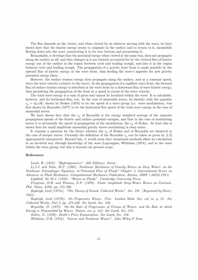
provides in equal parts the gradient in vertical flux and the temporal change in kinetic energy, asillustrated in Figure 2. The upwards vertical transport at the front of an advancing group providesfor increases in surface energy required there, and the reverse at the rear.

In the detailed analysis which follows, it is sufficient to know that for deep water gravity wavesin the absence of weak surface currents, to second order in wave steepness, see Li and Tulin (1996),equation 2.1.18.

η =

[1

2Aexpiβ +

i

2ω0Atexpiβ +

k0

4A2exp2iβ

]+ [CC] + 0(Ak)3 [2.3]

φ =

[−

icoA

2exp(k0y + iβ) + yAtexp(k0y + iβ)

]+ [CC] + 0(Ak)3 [2.4]

where A = aeiα(x,t); β = k0x−ω0t. The fluctuations of the slowly varying phase, α, is of higher orderthan that of the amplitude A.

2.2 Energy balance at the surface

At the surface, see [1.31], over the slow time, τ , appropriate to the modulation,

1

2

∂ρgη2

∂τ= Fn(K̂E; So) ·

ds

da[2.5]

where the overbar refers to averages over the fast time, t, characteristic of the waves themselves. Herewe consider only the consequences of [2.5] to the lowest relevant order, (Ako)

3. We have assumed that

τ

t= 0(Ak0)

−1 [2.6]

which is, indeed, characteristic of slow modulation arising from wave instability. To the lowest orderin the surface energy transfer, (Ako)

3, it is sufficient to represent η and φ by the underlined terms in[2.3] and [2.4].

To this lowest order,η = A cosφ [2.7]

9

~Fn(KE; So) ·ds

da= −ρφyφt/y=o [2.8]

and,φy = ekoyco [(Ako) sinβ + 2(Ako)ωoτ cosβ] [2.9]

φx = ekoyco [(Ak0) cos β] [2.10]

φt = ekoyc2o [(Ako)ωoτ sin β − (Ako) cosβ] [2.11]

Substituting [2.7] – [2.11] in [2.5], it is found that,

ρg

4(A2)τ = ρ

c3o

4(Ako)

2ωoτ [2.12]

which requires only that the linear dispersion relationship be satisfied:

ω20 = gk0 [2.13]

So the surface energy balance in itself, to order (Ak0)3, places no restrictions on the shape or speed

of a modulation, although it does require the linear dispersion relation [2.13], which is seen to providethe numerical balance in the energy exchange at the surface, [2.5].

2.3 Beneath the wave; the energy balance

The KE balance [1.4], which must apply at each point within the wave may be written

∂(ρq2/2)

∂τ+

∂(−ρφtφx)

∂χ+

∂(−ρφtφy)

∂y= 0 [2.14]

where χ is the “long” length scale, characteristic of the wave group length.Substituting from [2.9–2.11], we find for [2.14],

ρc2o

2

∂(Ako)2

∂τ+

ρc3o

2

∂(Ako)2

∂χ+

ρc2o

2

∂(Ako)2

∂τ= 0 [2.15]

This is seen to be satisfied for any modulation provided that,

∂

∂τ= −

co

2

∂

∂χ[2.16]

which is equivalent to [2.1] and [2.2], taking into account the substitution for slow variables. So, thekinetic energy balance is provided at every point beneath the wave for any modulation traveling athalf the phase speed. In this case it is easily seen that in the balance [2.14], the respective terms havethe relative magnitudes: −1; +2; −1. This confirms earlier claims illustrated in Figure 2.

Concluding Remarks

We have seen that the flux of wave kinetic energy is highly consequential for the physics of wavepropagation because of the interplay between the kinetic energy which occupies the body of the wave,and its potential energy, which resides in the surface both in its elevation (gravity) and in its surfacelength or area (surface tension).

10

The flux depends on the viewer, and when viewed by an observer moving with the wave, we haveshown here that the kinetic energy seems to originate in the surface and to return to it, meanwhileflowing down into the wave, penetrating it to its very bottom and permeating it.

Remarkably, it develops that the potential energy when viewed in the same way, does not propagatealong the surface at all, and that changes in it are entirely accounted for by the vertical flux of kineticenergy out of the surface in the region between crest and trailing trough, and into it in the regionbetween crest and leading trough. The propagation of a gravity wave front is made possible by theupward flux of kinetic energy at the wave front, thus feeding the wave’s appetite for new gravitypotential energy there.

However, the surface tension energy does propagate along the surface, and at a constant speed,twice the wave velocity (relative to the wave). In the propagation of a capillary wave front, the forwardflux of surface tension energy is absorbed at the wave front by a downward flux of wave kinetic energy,thus permitting the propagation of the front at a speed in excess of the wave velocity.

The total wave energy is a sum of parts and cannot be localized within the wave. It is calculable,however, and its horizontal flux, too. In the case of sinusoidal waves, its identity with the quantitycg = dω/dk, shown by Stokes (1876) to be the speed of a wave group (i.e. wave modulation), wasfirst shown by Reynolds (1877) to be the horizontal flux speed of the total wave energy in the case ofsinusoidal waves.

We have shown here that the cg of Reynolds is the energy weighted average of the separatepropagation speeds of the kinetic and surface potential energies, and that in the case of modulatingwaves it is necessarily the speed of propagation of the modulation, the cg of Stokes. At least this isshown here for small amplitude sinusoidal gravity waves modulating in deep water.

It remains a question for the future whether the cg of Stokes and of Reynolds are identical inthe case of steeper waves. Certainly the definition of the Reynolds cg can be taken as given by [1.3]appropriately interpreted. Beyond this, it would seem that variational methods allow its calculationin an involved way through knowledge of the wave Lagrangian, Whitham (1974), and in the wavewithin the wave group, but this is beyond our present scope.

References

Lamb, H. (1932). “Hydrodynamics”. (6th Edition). Dover.Li,J.J. and Tulin, M.P. (1995). Nonlinear Mechanics of Gravity Waves on Deep Water: on the

Nonlinear Schroedinger Equation, in“Potential Flow of Fluids” Chapter 3, International Series onAdvances in Fluid Mechanics, Computational Mechanics Publication, Boston, ISBN 1.56252.279.5.

Lighthill, Sir M.J. (1978). “Waves in Fluids”. Cambridge University Press.Peregrine, D.H. and Thomas, G.P. (1979). Finite Amplitude Deep-Water Waves on Currents.

Phil. Trans. A292, pp. 371-390.Rayleigh, Lord (1877a). “The Theory of Sound: Collected Works”. Sec. 191. (Reprinted by Dover,

1945).Rayleigh, Lord (1877b). On Progressive Waves. Proc. London Math. Soc. vol. ix, p. 21. See

Collected Works, Part I, pp. 475-480. See Lamb, Sec. 236.Reynolds, O. (1877). On the Rate of Progression of Groups of Waves, and the Rate at which

Energy is Transmitted by Waves. Nature, xvi, p. 343. See Lamb, Sec. 237.Stokes, G. (1876). Smith’s Prize Examination. See Lamb, Sec. 236.Whitham, G.B. (1974). “Linear and Nonlinear Waves”. John Wiley & Sons.

11

Figure 1: Kinetic Energy Flux under Monochromatic Waves.

12

Figure 2: Kinetic Energy Balance within a Wave Group, Schematic.

13