- : , . , , , , ,

ELSEVIER Journal of Statistical Planning and

Inference 52 (1996) 67-75

Jstat °umal°f istical planning

and inference

On the stability of biased estimates and the regularization method

Hu Yang Institute of Statistics and Mathematics, Chongqing Jiaotong University, Chongqing 630074, Peoples'

Republic of China

Received 20 February 1992; revised 25 February 1995

Abstract

The present paper purports to investigate the stability of the biased estimates based on the stable solutions in the corresponding equation, and mainly discusses the regularization method, the stable estimate and some related problems.

,4MS Subject Classification: 62H12, 62J05, 65K10

Key words: Quasi-regular solution; Stable estimate; Minimization problem

1. Introduction

Consider the multivariate linear model

y i j=Xi l f l l j+x i2 f l2 j+ . . .WXip f lp j+g i j , i = 1 , 2 ..... n j = l , 2 ..... m, (1.1)

where Yo and Xik (i = 1,2,...,n, j = 1,2 .... ,m, k = 1,2 ..... p) are, respectively, the observat ion values of the response and independent variables, flkj the parameters, and

eq the regression errors. Denot ing Y=(Yi~) . . . . X=(Xik),×p, fl=(flkj)p×m, e. = (e~) . . . . (1.1) can be briefly expressed as Y = Xfl + e; here X is called the design

matrix. We often suppose the row vectors of e uncorrelated with one another, and possess mean value zero and the same covariance matrix S. For the multivariate

linear model (1.1), there are many different methods used to estimate ft. For example, when 2" is positive-definite matrix and rank R ( X ) = p, the best linear unbiased estimate ( B L U E ) i s f l = ( X v X ) - I X T Y . Let vec/~=(/~IT,/~ 2r ..... /~mT)T [here

/~ _- (/~1,fi2 ..... /~m)l, then the mean squared error (MSE) i s

P

MSE(vec/~) = t r [Cov(vec/~)] = t r [ S ® ( x T x ) -1] = ( t rS) ~ ,~/- 1, (1.2) i = l

0378-3758/96/$15.00 © 1996--Elsevier Science B.V. All rights reserved SSD! 0 3 7 8 - 3 7 5 8 ( 9 4 ) 0 0 0 2 4 - 0

68 Hu Yang / Journal of Statistical Planning and Inference 52 (1996) 67-75

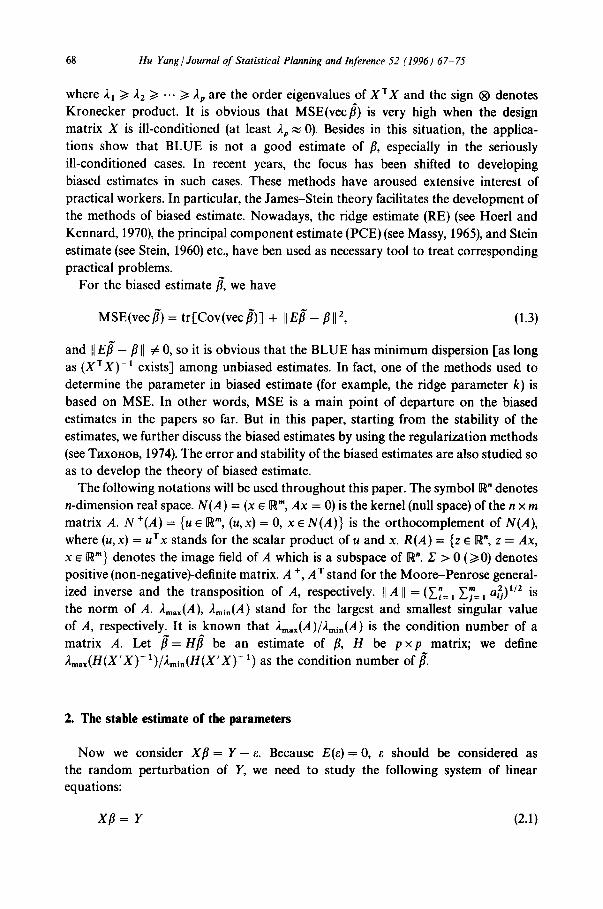
where 21/> 22/> .-. ~> 2p are the order eigenvalues of X r X and the sign ® denotes Kronecker product. It is obvious that MSE(vec/~) is very high when the design matrix X is ill-conditioned (at least 2p ~ 0). Besides in this situation, the applica- tions show that BLUE is not a good estimate of/~, especially in the seriously ill-conditioned cases. In recent years, the focus has been shifted to developing biased estimates in such cases. These methods have aroused extensive interest of practical workers. In particular, the James-Stein theory facilitates the development of the methods of biased estimate. Nowadays, the ridge estimate (RE) (see Hoerl and Kennard, 1970), the principal component estimate (PCE) (see Massy, 1965), and Stein estimate (see Stein, 1960) etc., have ben used as necessary tool to treat corresponding practical problems.

For the biased estimate/~, we have

MSE(vec/~) = tr[Cov(vec/~)] + II E/~ - fl II 2, (1.3)

and I[ E/~ - fl II ~ 0, so it is obvious that the BLUE has minimum dispersion [as long as (XrX) - 1 exists] among unbiased estimates. In fact, one of the methods used to determine the parameter in biased estimate (for example, the ridge parameter k) is based on MSE. In other words, MSE is a main point of departure on the biased estimates in the papers so far. But in this paper, starting from the stability of the estimates, we further discuss the biased estimates by using the regularization methods (see TnxonoB, 1974). The error and stability of the biased estimates are also studied so as to develop the theory of biased estimate.

The following notations will be used throughout this paper. The symbol R" denotes n-dimension real space. N ( A ) = (x ~ R" , A x = 0) is the kernel (null space) of the n x m matrix A. N +(A) = {u e R m, (u,x) = O, x ~ N(A)} is the orthocomplement of N (A) ,

where (u, x) = u r x stands for the scalar product of u and x. R ( A ) = {z ~ ~", z = Ax ,

x e R"} denotes the image field of A which is a subspace of R". ,~ > 0 (/>0) denotes positive (non-negative)-definite matrix. A +, A r stand for the Moore-Penrose general-

" " a2) 1/2 is ized inverse and the transposition of A, respectively. IIA [I = (Yi=l ~#=1 the norm of A. 2m~x(A), 2mln(A) stand for the largest and smallest singular value of A, respectively. It is known that 2m,x(A)/2mi,(A) is the condition number of a matrix A. Let /~= H/{ be an estimate of fl, H be p x p matrix; we define 2max(H(X'X)-l)/2min(H(X'X)-1) as the condition number of/L

2. The stable estimate of the parameters

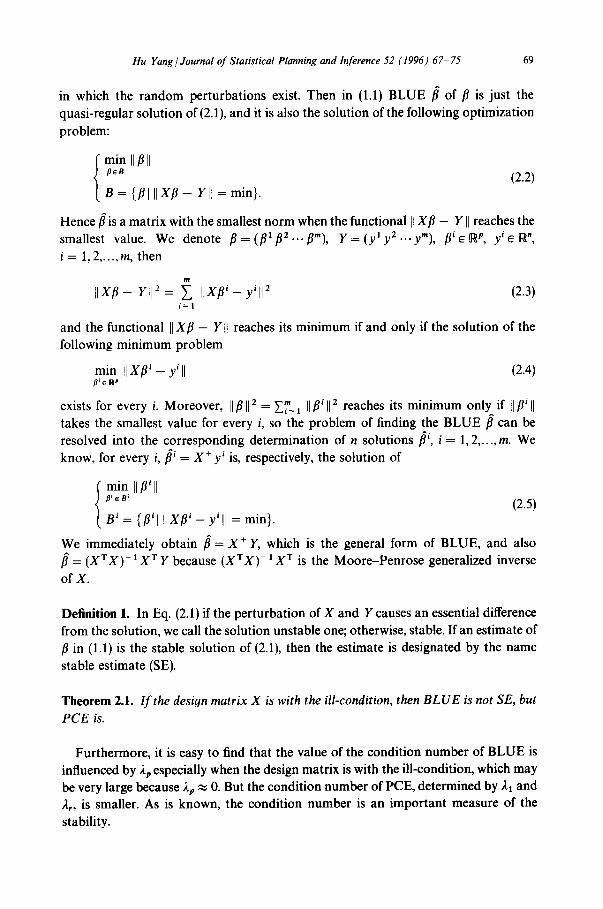
Now we consider X/~ = Y - ~ . Because E(e)= 0, e should be considered as the random perturbation of Y, we need to study the following system of linear equations:

Xf l = Y (2.1)

Hu Yang / Journal of Statistical Planning and Inference 52 (1996) 67- 75 69

in which the random perturbations exist. Then in (1.1) BLUE /~ of 8 is just the quasi-regular solution of (2.1), and it is also the solution of the following optimization problem:

m i n II 8 II p~a (2.2)

B = { t l IIX8 - YII = min}.

Hence/~ is a matrix with the smallest norm when the functional 11X8 - Y II reaches the smallest value. We denote 8 = (81 8 2 "'" tim), y = (yl),2 . . . y m ) , fli 6 ~p, yi ~ Rn,

i = 1, 2 ..... m, then

r n

[IX8 - El i 2 = ~, I I X 8 ' - y'll 2 (2 .3 ) i = 1

and the functional II X 8 - Y I[ reaches its minimum if and only if the solution of the

following minimum problem

min II X 8 i - yi II (2.4)

exists for every i. Moreover, II t II 2 __ ~i'-- 1 II t i II 2 reaches its minimum only if [I 8 i II takes the smallest value for every i, so the problem of finding the BLUE/~ can be resolved into the corresponding determination of n solutions if, i = 1, 2 ..... m. We know, for every i, f f = X + yi is, respectively, the solution of

m i n II t i II a'~B' (2.5) n i : {8'1 llXS'-- Y'II : min}.

We immediately obtain /~ = X + Y, which is the general form of BLUE, and also = ( X T X ) - 1 X T y because ( X r X ) - I X r is the Moore-Penrose generalized inverse

of X.

Definition 1. In Eq. (2.1) if the perturbation of X and Y causes an essential difference from the solution, we call the solution unstable one; otherwise, stable. If an estimate of fl in (1.1) is the stable solution of (2.1), then the estimate is designated by the name stable estimate (SE).

T h e o r e m 2 . 1 . I f the design mat r i x X is with the ill-condition, then B L U E is not SE, but

P C E is.

Furthermore, it is easy to find that the value of the condition number of BLUE is influenced by 2p especially when the design matrix is with the ill-condition, which may be very large because 2p ~ 0. But the condition number of PCE, determined by 21 and 2r, is smaller. As is known, the condition number is an important measure of the stability.

70 Hu Yang / Journal of Statistical Planning and Inference 52 (1996) 67- 75

With reference to (2.1), if there is a per turbat ion e for Y, the quasi-regular solution of fl will be a solution of the following optimization problem:

rain II/~ II a~B (2.6)

B = { ~ RPx R ' ] I t X n - YII ~ I1~11}.

In other words, we have to determine the minimum of the quadrat ic functional f(/~) = II/~ II 2 when II X/~ - Y I[ ~< I[ ~ It. Equivalently, we only need to determine the minimum of F(fl i) when IIX/~ ~ - Yi[I ~< I1~11 for every i, where e = (el,e 2 ..... era). In order to obtain the quasi-regular solution of (2.1) [it is obvious that. the solution is SE in (1.1)-I, we first establish a lemma which shows that the inequality sign of (2.6) may be replaced by the equality sign.

Lemma. I f IIX~ ~ - yi[I ~ II~ill, then the functional F(fl i) reaches its minimum at the

boundary IIX/3 ~ - Y~II = I1~11, i = 1,2 ..... m.

Proof. Let II 8 `0 II 2 : mina, , B, II ~i II 2 > 0, Bi = (fit ~ RPl II XB ~ - Y~ II ~ II ~i II) and = IIX/~ '°- yil[ <~ [1~'11, i= 1,2 ..... m, and denote

( , l ~ ' l , - 6 ) f f = m i n 1, IlXll l~r°ll ' i = 1,2 ..... m. (2.7)

If/~i = (1 - i f ) i f° , we can show that

I l X f f - f l l l ~< IIX#'°-y'll +/~llXII II/~'°11 ~< I1~'11, i = 1,2 ..... m (2.8)

and

Ilffll = ( 1 -~a)211/~'°112 < Ilffoll 2, i = 1,2 . . . . . m. (2.9)

Hence for the quadrat ic functional F in the set Bi, the vector flio is not the solution of the minimization problem, with flio satisfying the condit ion I[ X f f ° - Y~ II < II ~i II for every i. The Lemma is established. []

Theorem 2.2. Considering the model (1.1), there exists a constant c such that

fl~ = ( c X T X + I ) - l c X r Y

is the quasi-regular solution of(2.1), so it is SE of ft.

(2.1o)

Generally, we call/~c = ( c X T X + I ) - l cXT Y the general (narrow sense) SE of fl for arbi t rary constant c. It is obvious that SE ffc is RE when c > 0. So it shows that RE is the stable numerical solution of (2.1) and SE of fl in (1.1). Fur thermore , for a system of linear equations with the ill-condition, because the condit ion number z ( X r X + (1/c)I) ~< z (XXX) . RE is the solution obtained from the system of linear

Hu Yang / Journal of Statistical Planning and Inference 52 (1996) 67 75 71

equations [see (5.7) in Section 5 of this paper] which are not with the ill-condition (or only possess the slight ill-condition) by lowering the condition number. Certainly, it is more stable and less influenced by the random perturbation than BLUE.

3. SE approximation of B L U E

Now, we establish an estimate of the differences/~ - / ~ between the general SE and BLUE. Because

fl~ = ( c X T X + I ) - X c X T X f l , f i e N + ( X ) , (3.1)

let e~, e2 ..... epe N + ( X ) be the corresponding orthogonal eigenvectors of the eigen- values 2x, 22 ..... 2p, which make up a group of orthogonal basis of N + ( X ) and

X T X e i = 2iei, V i (3.2)

denoting/~ = 52~'= x otiei, in which ~i is a constant for every i. Then from (3.1), we have

~, c 2 i ~ tic = c21 + 1 el. (3.3)

i = 1

Because 11~l12=E,L~c22,21~,12(o~,+1)-2, it is obvious that l im¢o~ /~=

52~=~ ~,e, = / ~ and tl/~ll increasingly converge to [I/~11. While

P 0~ i

L - fl = -- E c2i +~--1 e,, (3.4) i = 1

SO

~=1 Oti X e i : - - ~ °~ix//~i X(f lc - fl) = --i= c21 +-----~ i=1 c2i + ~ e,, (3.5)

hence the functional

°t221 (3.6) • (c) = II x ( /~c - fi)II "2 = (c~., -t- 1) 2

i = 1

is monotone decreasing and

P

+(C)lc=O = Z ~ ~., = (xT xIL fi) = II X/~ll ~, (3.7) i = l

• (C) lc~ = 0.

Thus, the functional ~(c) is monotone decreasing in the interval [0, + oo) and its value is between 0 and II 1711- Further, we can obtain an upper bound of [[fl~ - fill.

Theorem 3.1. Le t to e N + ( X T) be a vector sat is fying x T co = -- fl, then

II/~c-/~11 ~< IIXTII I1~11 + II~,ll/,,/~. (3.8)

72 Hu Yang / Journal of Statistical Planning and Inference 52 (1996) 67- 75

4. Generalized SE and the approximation of PCE

Definition 2. Let C be a p x p matrix, then

if(C) = (CXTX + I)- ~ CX r Y ~ H(C)fl (4.1)

is called the generalized SE.

It is obvious that/~(C) is equal to/~c when C = cI (c is a constant). As a special case, we only consider that C and X r X can have simultaneous diagonlization, so that there is an orthogonal matrix Q such that QrCQ =diag(c l ,c2 ..... Cp), Qr XTXQ =

diag(21,22,..., 29). Then

H(C) = (CXTX + I)- 1CXTX

= Q(QrCQQTXTXQ + 1)-IQrCQQTXTXQQT

, . [ c121 c222 C,2p ) --Q°'ag~c,]-~l ~ - 1 ' C 2 2 2 + 1 . . . . . CpAp+l QT.

(4.2)

Because c~, i = 1,2 ..... p are the eigenvalues of C, if C > 0, denoting kl = ci-1, i = 1,2 ..... p, K ~ QTc-1Q = diag(kl,k2 ..... kp), then /~(C) = ( X r X + K ) - I X r Y , that is GRE [generalized ridge estimate, see Hoerl and Kennard (1970)]. But if 21 ~ 0, i = r + 1, r + 2,..., p [namely the design matrix of (1.1) is with the ill-condition], we select

b(1 - b)-12i -1, i = 1,2,...,r, (4.3) ci= O, i = r + l ,r + 2 ..... p,

then/~(C) is the Sclove shrunken estimate (see Sclove, 1968) for every definite constant b, and when b ~ 1, it increasingly approximates Massy PCE, which omits the back p - r principal components. It is obvious that the condition number of/~(C) keeps unchanged for the whole limit process, namely/if(C) will stably increase to its limit estimate PCE when b ~ 1. But GRE does not possess this property.We know that the condition number of GRE will tend to infinity when k ~ + ~ . In this case, the approximation of PCE is unstable.

Moreover, selecting special cl < 0 can bring down the condition number and make better BLUE. In fact, letting

c i = - ( 2 i - 2 / x - ~ ) -1, Vi, 0 < a < l , (4.4)

the velocity of change on H(C) is 2 a, and its condition number (212~ 1)a~ l(a ~ 0). But at 2 = 1, we can select a larger number to substitute, whose influence is very little upon the stability of the solution.

Hu Yang / Journal of Statistical Planning and Inference 52 (1996) 67- 75 73

5. Proofs of main theorems

Proof of Theorem 2.1. Because 21 >/22/> ..- >/2j, are the eigenvalues of x T x , there exists an orthogonal matrix P such that p T x T x p = diag(21,22 ..... 2p). Denoting ¢~ = pTXTy, = (~i, ~ .. . . . ¢~)T, the regular solution of (2.1)is/~' & ( /~ , /~ ..... /~)r for

^ every i, and we have fl~ = ~ 2 k 1 for every k, then

11/~'11 = , , P T f f I , = [ k__~l (~2k 1)2] 1/2. (5.1)

It is easy to find/~i is not a stabe solution of (2.1) because 2p ~ 0 at least when the design matrix is with the ill-condition. Obviously, BLUE is not SE. Also, if the (r + 1)th eigenvalue is the first one which is approximately equal to zero, i.e. 2,+ ~ ~ 0, then partitioning P: P = (P~ P2), where P1 is a p x r matrix, PCE of fli may be expressed as ffi = Pt P~ f f . While

pT(xTx)- 1 p = diag(2 ( 1, 22 x ..... 2~- 1 ),

we have

p I ( x T x ) - t P = °° ) 0...0

0...27 1 0...0

and

P r l ( X T X ) - t PC' = (2i- ~ ~ , 221 ~ ..... 27 ,~)T

II f f II ~ II P ~ f f 11 = II P ~ ( x T x ) - ' X T y ' II = II P~[(XTX) -1 PC' II

= ( ~ 2 k l ) 2 <~ I IpTxTy I I /A , = I IxTyI[ /2 , . k = l

[] It is obvious that PCE is SE. Theorem 2.1 is established.

(5.2)

(5.3)

Proof of Theorem 2.2. By the general regularization method [see TnxonoB, 1974), we can change (2.1) into the minimization problem (2.6), equivalently into the following minimization problem:

min f(fl i) p'EB, (5.4) ni = {fli e RPl [IXfl i - yill = Ilgll}.

for every i, where F(fl ~) = II//~ II 2. In order to determine their stable solution, using the Lagrange multiplier c, we substitute the above problem for the following minimiz- ation problem of the functional:

O(fl~,Yi, c , X ) = c ( l lX# ~ - yill - IIg[I) + F(/~), (5.5)

74 Hu Yang / Journal of Statistical Planning and Inference 52 (1996) 67-75

where c is a constant determined by the boundary condit ion IIX/~ i - YiH = II~ill. Minimizing the functional (5.5) is equivalent to solving the system of equations

( c X T X + l)fl i = cXTy i, i = 1,2 ..... m. (5.6)

In (5.6), when c is fixed, there is a stable numerical solution as follows:

i l l= ( c X T X + i ) - l c X T y i , i = 1,2 ..... m; (5.7)

corresponding/~c = (cX T X + I ) - 1 cX T y is SE of ft.

P roof of Theorem 3.1. Denoting /~c = Hc Y, and Jet Yo be a practical value of the response variable,/~o = H~ Yo; then

L - / ~ = ( L - ~o) + (~,.o - ~) = u c ( r - Vo) + (tL - t~). t5.8)

Since II/~cll 2 increasingly converges to II/~[I 2, it is easy to show IIHcll < I[X + II and

I I n ~ ( Y - Yo)ll ~< [IS+ll I1~11- (5.9)

Now, we estimate the second term of (5.8); from the proof of Theorem 2.2

/~-o = min 0(fl, Yo, c, X), (5.10)

so we have

c(X/~.o - Yo,Xu) + (/ff~o, u) = 0 (5.11)

for every u ~ R p. Let t =/~co - / ~ ; expression (5.11) is changed into

c(Xt, Xu) + (t + fl, u) = O, u ~ R p, (5.12)

here X/~= Yo. But /~eR(XT), So there exists a unique t o e N + ( X T) satisfying xT to = --]~, and we have

(cXt - c~, Xu) + (t, u) = O, u e R P. (5.13)

Hence, the functional O(fl, c-~o9, c, X ) reaches its minimum at t, namely

O(t,c lto, c,X)<~ O(s,c-l to, c ,X) , V s e R p. (5.14)

Especially, when s = 0,

H/~o-/~11 = Iltll ~< Iltold/x/~. (5.15)

Theorem 3.1 is established from (5.9) and (5.15). []

Hu Yang / Journal of Statistical Planning and Inference 52 (1996) 67-75 75

Acknowledgements

The author would like to acknowledge the referee for his careful reading of the manuscript and useful comments.

References

Hoerl, A.E., R.W. Kennard (1970). Ridge regression: biased estimation for non-orthgonal problem & ap- plication for non-orthogonal problems. Technometrics 12, 55-82.

Massy, W.F. (1965). Principal component regression in exploratory statistical research. JASA 60, 234 266. Sclove, S.L. (1968). Improved estimators for coefficients in linear regression. JASA 63, 597-606. Stein, C.M. (1960). Multiple regression. In: I. Olkin, Ed., Contributions to Probability and Statistics. Essays

in Honor of Harold Hotelling, Stanford University Press, Stanford. THXOHOB, A.H., B.$1. Ap6enxn. (1974). MeTo~r PeMeHH~I HeEoppeKrnrx 3a~Iau, HayKa, Moci<Ba.