On the solvability and the inviscid limit of Cauchy ...

On the solvability and the inviscid limit of

Cauchy problems for certain classes of the

non-linear Schrodinger equation

Doctoral Thesis

Nikolaos Gialelis

Department of Mathematics,National and Kapodistrian University of Athens,

Athens, Greece2019

This research is co-financed by Greece and the European Union (European Social Fund- ESF)through the Operational Programme “Human Resources Development, Education and LifelongLearning” in the context of the project “Strengthening Human Resources Research Potential viaDoctorate Research” (MIS-5000432), implemented by the State Scholarships Foundation (IKY).

Advisory committee

Dimitri J. Frantzeskakis - Department of Physics, National and Kapodistrian University of AthensNikolaos I. Karachalios - Department of Mathematics, University of the AegeanIoannis G. Stratis (supervisor) - Department of Mathematics, National and Kapodistrian Univer-sity of Athens

Dissertation Examining Committee

Nicholas D. Alikakos - Department of Mathematics, National and Kapodistrian University ofAthensGerassimos Barbatis - Department of Mathematics, National and Kapodistrian University ofAthensPanagiotis Gianniotis - Department of Mathematics, National and Kapodistrian University ofAthensPandelis Dodos - Department of Mathematics, National and Kapodistrian University of AthensDimitri J. Frantzeskakis - Department of Physics, National and Kapodistrian University of AthensNikolaos I. Karachalios - Department of Mathematics, University of the AegeanIoannis G. Stratis - Department of Mathematics, National and Kapodistrian University of Athens

Contents

Abstract vi

1 Preliminaries 11.1 Notation . . . . . . . . . . . . . . . . . . . . . . . . . . . . . . . . . . . . . . . . . . . . . 11.2 Definitions and basics . . . . . . . . . . . . . . . . . . . . . . . . . . . . . . . . . . . . . 1

1.2.1 Second-order, symmetric, uniformly elliptic operators . . . . . . . . . . . . . 21.2.2 Restriction and extension-by-zero operators . . . . . . . . . . . . . . . . . . . 41.2.3 Uniformly Lipschitz boundaries . . . . . . . . . . . . . . . . . . . . . . . . . . . 71.2.4 The continuous Sobolev embeddings . . . . . . . . . . . . . . . . . . . . . . . . 81.2.5 The compact Rellich-Kondrachov embeddings . . . . . . . . . . . . . . . . . . 91.2.6 Uniformly m-Lipschitz boundaries . . . . . . . . . . . . . . . . . . . . . . . . . 101.2.7 The Leibniz formula . . . . . . . . . . . . . . . . . . . . . . . . . . . . . . . . . 111.2.8 Change of variables . . . . . . . . . . . . . . . . . . . . . . . . . . . . . . . . . . 131.2.9 Difference quotients . . . . . . . . . . . . . . . . . . . . . . . . . . . . . . . . . . 171.2.10 Chain rule . . . . . . . . . . . . . . . . . . . . . . . . . . . . . . . . . . . . . . . 201.2.11 Cut-off functions . . . . . . . . . . . . . . . . . . . . . . . . . . . . . . . . . . . . 231.2.12 Elliptic regularity theory for m-Lipschitz boundaries . . . . . . . . . . . . . . 24

2 Non-vanishing solutions of the defocusing NLSE 382.1 Introduction . . . . . . . . . . . . . . . . . . . . . . . . . . . . . . . . . . . . . . . . . . . 382.2 Formulation of the problem . . . . . . . . . . . . . . . . . . . . . . . . . . . . . . . . . . 38

2.2.1 A general non-linear operator . . . . . . . . . . . . . . . . . . . . . . . . . . . . 392.2.2 A special case of the non-linear operator . . . . . . . . . . . . . . . . . . . . . 412.2.3 The non-linear operator on restrictions . . . . . . . . . . . . . . . . . . . . . . 45

2.3 Weak solutions . . . . . . . . . . . . . . . . . . . . . . . . . . . . . . . . . . . . . . . . . 462.3.1 Local existence results . . . . . . . . . . . . . . . . . . . . . . . . . . . . . . . . 462.3.2 Uniqueness and globality . . . . . . . . . . . . . . . . . . . . . . . . . . . . . . . 632.3.3 Conservation of energy and well posedness . . . . . . . . . . . . . . . . . . . . 65

2.4 Regularity of solutions . . . . . . . . . . . . . . . . . . . . . . . . . . . . . . . . . . . . . 67

3 The inviscid limit of the linearly damped and driven NLSE 773.1 Introduction . . . . . . . . . . . . . . . . . . . . . . . . . . . . . . . . . . . . . . . . . . . 773.2 Formulation of the problem . . . . . . . . . . . . . . . . . . . . . . . . . . . . . . . . . . 773.3 Weak existence results . . . . . . . . . . . . . . . . . . . . . . . . . . . . . . . . . . . . . 783.4 NLSE as limit case of linearly damped and driven NLSE . . . . . . . . . . . . . . . . 82

Bibliography 86

v

Abstract

The non-linear (in particular the semi-linear) Schrodinger equation, very often referred to by theacronym NLSE, is a universal model describing the evolution of complex field envelopes in non-linear dispersive media; it appears in a variety of physical contexts, ranging from optics to fluiddynamics and plasma physics, and it has attracted a huge interest from the rigorous mathematicalanalysis point of view, as well. The importance of the NLSE model is not restrained to the case ofconservative systems, but it is also associated to dissipative models. Many of the closely connectedto the NLSE pattern formation phenomena, emanate via the genesis of localized structures withfinite spatial support, or with sufficiently fast spatial decay, the so-called solitons. Among thevarious types of waves whose amplitude is modulated, there are two principal kinds of solitons,depending on the category of the non-linearity; in the case of an attractive (or focusing) medium,the non-linearity causes the formation of structures termed “bright solitons”, while in the case ofa repulsive (or defocusing) medium, the non-linearity generates “dark solitons” (i.e., non-linearsolitary waves having the form of localized dips in density, that decay off of a continuous-wavebackground; if the density of the dip tends to zero, the dark solitons are named “black”; otherwise“grey”).

Theoretical physical studies on dark solitons started in 1971, by the work of T. Tsuzuki [45] inthe context of Bose-Einstein condensates. Two years later, in [50], V. E. Zakharov and A. B. Shabatdemonstrated the complete integrability of the defocusing NLSE utilizing the Inverse ScatteringTransform (incidentally, the same authors had shown the integrability of the focusing NLSE in[49]). The progress in the theory after that was very rapid and immense. As for experimentalresults, the progress was equally impressive: after the “early age” experiments of the 1970s, the“new age”, that emerged in the middle of the first decade of the 21st century, is a period ofspectacular progress. These led to a vast amount of literature. A detailed presentation of thephysical studies (theoretical and experimental) and of the recent progress regarding the defocusingNLSE is contained in [33], that incorporates an extensive bibliography.

Regarding the rigorous mathematical analysis of the NLSE, the books [6], [10], [11], [42], [43]are classical by now. The more recent books [14], [17], [36], also contribute substantially to thefield. The reference lists in all these books are representative of the huge interest and amount ofresearch work on the NLSE.

In this doctoral thesis, we are interested in two problems involving the NLSE. The first one isthe quest for and the study of a special type of solutions of the defocusing NLSE which do notvanish at the spatial extremity. The second one is the study of the “inviscid limit” of the linearlydamped and driven NLSE. Below follows a brief presentation of both the questions that we raise,as well as the conclusions that we reach.

Non-vanishing solutions of the defocusing NLSE. For an interval J0 ⊆R with 0 ∈ J0 , anopen U ⊆Rn, a differentiable a= (aij)ni,j=1 ∶ U → Cn×n, as well as a twice-differentiable ζ ∶ U → Cwhich survives at the boundary or at infinity, we search for a twice-differentiable u ∶ J0×U → Cthat solves the n-dimensional initial/“boundary”-value problem for the NLSE with pure powernon-linearity

⎧⎪⎪⎪⎪⎪⎨⎪⎪⎪⎪⎪⎩

i∂u∂t− div(aT∇(u+ζ)) + λ (∣u+ζ ∣α+r) (u+ζ) = 0, in J∗0 ×U

u = u0, in t=0×Uu = 0, in J0×∂U, and u

∣x∣∞ÐÐÐ→ 0, in J0×U,(1)

for λ∈R∗, α∈(0,∞) and r∈R. The above problem arises from the search for solutions of the form

v(t, x)=e−iλrt (u(t, x)+ζ(x))

vi

CONTENTS vii

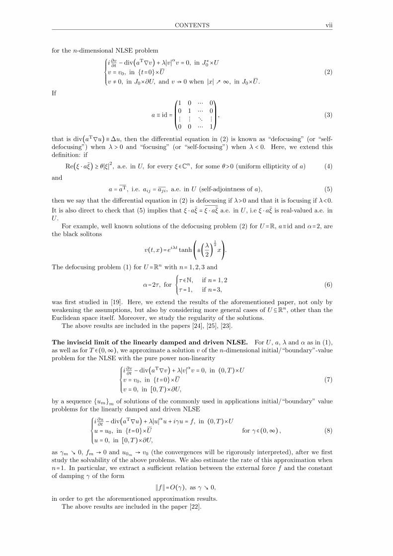
for the n-dimensional NLSE problem

⎧⎪⎪⎪⎪⎨⎪⎪⎪⎪⎩

i∂v∂t− div(aT∇v) + λ∣v∣αv = 0, in J∗0 ×U

v = v0, in t=0×Uv ≠ 0, in J0×∂U, and v ↛ 0 when ∣x∣∞, in J0×U.

(2)

If

a ≡ id =⎛⎜⎜⎜⎝

1 0 ⋯ 00 1 ⋯ 0⋮ ⋮ ⋱ ⋮0 0 ⋯ 1

⎞⎟⎟⎟⎠, (3)

that is div(aT∇u) ≡∆u, then the differential equation in (2) is known as “defocusing” (or “self-defocusing”) when λ > 0 and “focusing” (or “self-focusing”) when λ < 0. Here, we extend thisdefinition: if

Re(ξ ⋅ aξ) ≥ θ∣ξ∣2, a.e. in U, for every ξ ∈Cn, for some θ>0 (uniform ellipticity of a) (4)

and

a = aT, i.e. aij = aji, a.e. in U (self-adjointness of a), (5)

then we say that the differential equation in (2) is defocusing if λ>0 and that it is focusing if λ<0.

It is also direct to check that (5) implies that ξ ⋅ aξ = ξ ⋅ aξ a.e. in U , i.e ξ ⋅ aξ is real-valued a.e. inU .

For example, well known solutions of the defocusing problem (2) for U =R, a≡ id and α=2, arethe black solitons

v(t, x)=eiλt tanh⎛⎝±(λ

2)

12

x⎞⎠.

The defocusing problem (1) for U =Rn with n= 1,2,3 and

α=2τ, for

⎧⎪⎪⎨⎪⎪⎩

τ ∈N, if n= 1,2

τ =1, if n=3,(6)

was first studied in [19]. Here, we extend the results of the aforementioned paper, not only byweakening the assumptions, but also by considering more general cases of U ⊆Rn, other than theEuclidean space itself. Moreover, we study the regularity of the solutions.

The above results are included in the papers [24], [25], [23].

The inviscid limit of the linearly damped and driven NLSE. For U , a, λ and α as in (1),as well as for T ∈(0,∞), we approximate a solution v of the n-dimensional initial/“boundary”-valueproblem for the NLSE with the pure power non-linearity

⎧⎪⎪⎪⎪⎨⎪⎪⎪⎪⎩

i∂v∂t− div(aT∇v) + λ∣v∣αv = 0, in (0, T )×U

v = v0, in t=0×Uv = 0, in [0, T )×∂U,

(7)

by a sequence umm of solutions of the commonly used in applications initial/“boundary” valueproblems for the linearly damped and driven NLSE

⎧⎪⎪⎪⎪⎨⎪⎪⎪⎪⎩

i∂u∂t− div(aT∇u) + λ∣u∣αu + iγu = f, in (0, T )×U

u = u0, in t=0×Uu = 0, in [0, T )×∂U,

for γ ∈(0,∞) , (8)

as γm 0, fm → 0 and u0m → v0 (the convergences will be rigorously interpreted), after we firststudy the solvability of the above problems. We also estimate the rate of this approximation whenn=1. In particular, we extract a sufficient relation between the external force f and the constantof damping γ of the form

∥f∥=O(γ), as γ 0,

in order to get the aforementioned approximation results.The above results are included in the paper [22].

viii CONTENTS

Even though the techniques employed here can be used to deal with additional cases of non-linearities, such as the saturated one, we choose to present the results only for the case of purepower non-linearity. This is due to the fact that this kind of non-linearity is the commonest inapplications, and also acts as the model case for every other potential non-linearity.

We also emphasize that we present here an alternative technique for the existence results in theweak sense, in both bounded and unbounded sets, that differs from the classical one of “regularizednonlinearities” presented in [10] (see Theorem 3.3.5 therein). As we show here, this technique notonly allows us to rigorously derive an estimate for the energy of the solutions, but it also canbe applied to derive regularity results for the solutions. We note that the aforementioned energyestimate is formally obtained (this is what is done in a plethora of published papers), by takingthe scalar product with i∂u

∂t. However, for a weak solution, i.e. a solution with values in H1

0(U),∂u∂t

belongs merely to H−1(U), and thus this practice is not justified.As far as the regularity of the solutions is concerned, we highlight that the applicability of the

above technique passes through the exact determination of the dependence of the elliptic regularityestimates from the properties of an appropriate set in which the second-order elliptic problem isconsidered. That drives us to review the whole regularity theory for a special (yet quite large)class of appropriate sets, which we call sets with uniformly m-Lipschitz boundaries, for m∈N. Thisreview, along with a presentation of useful, already known and new results from the theory of theSobolev spaces, is included in the introductory first chapter of the present thesis.

Chapter 1

Preliminaries

1.1 Notation

We start with some notation used throughout the thesis:

1. We write C for any positive constant. Such a constant may be explicitly calculated in termsof known quantities and may change from line to line and also within a certain line in a givencomputation. We also employ the letter K for any increasing function K ∶ [0,∞]m → (0,∞],for some m∈N.

2. When an element appears as subscript in an other element, the first one denotes that thesecond one depends on it, while its absence designates either independence or “harmless”dependence. We also apply the classic method of writing an element as a function of anotherone, in order to denote an dependence. The presence of the subscript ⋅w to a differentialoperator for “space”-variables indicates that we consider the operator with the weak (i.e.distributional) sense, while the absence indicates differentiations of the ordinary sense.

3. We write U for any non-empty open ⊆Rn, as well as J for any non-empty open interval. If,in addition, 0∈J we write J0 for every such interval. We also define F(U) to be the spaceof functions with U for their domain.

4. If u∈F(U ;C) and also every derivative, in some sense S, of the kth order (k ∈N0), i.e. everyDαSu, with α ∈Nn0 and ∣α∣ = k, exists, then ∇kSu stands for the vector of components those

derivatives. Moreover, if u∈F(U ;Cm), for m∈N, and also every ∇Suj , for j= 1, . . . ,m, exists,we then write JSu for the Jacobian matrix, i.e.

JSu ∶= (∂iSuj)j=m,i=nj,i=1

∈ F(U ;Cm×n),

as well as det(JSu) for its determinant. The Jacobian matrix is essential for the change ofvariables formula (see, e.g., Theorem 9.52 in [35]), which plays essential role for us here.

5. For every m∈N, Xm(U) stands for the Zhidkov space over U , defined as the Banach space

Xm(U) ∶=u∈L∞(U) ∣∇kwu∈L2(U), for k= 1, . . . ,m ,equipped with its natural norm. A typical example is tanh ∈⋂∞m=1X

m(R). We note thatthe first version of such spaces over R is introduced in [51] and a generalization for higherdimensions (along with certain modifications) is done in [52], [18], [20] and [19]. Here, weconsider Xm over any U .

6. Following the notation of, e.g., [15] and [44], if u ∶ J ×U → C, with u(t, ⋅) ∈F(U) for eacht ∈ J , then we associate with u the mapping u ∶ J → F(U), defined by [u(t)](x) ∶= u(t, x),for every x∈U and t∈J . For the weak derivative (when it exists) of the “time”-variable of afunction-space-valued function u, we simply write u′.

1.2 Definitions and basics

Here, we critically review some useful, already known definitions and results, and we provide newones.

1

2 1.2. DEFINITIONS AND BASICS

1.2.1 Second-order, symmetric, uniformly elliptic operators

The characterization “uniformly” is used in [15]. Other adverbs also used in the bibliography are,e.g., “strictly” in [26] and “strongly” in [38].

Definition 1.2.1. For a=(aij)ni,j=1 ∈L∞(U) satisfying (4) and (5), we write

Lw =Lw(a, θ) ∶ u∈Lp(U) for some p∈[1,∞] ∣∇wu∈L2(U)→H−1(U)

for the linear and bounded operator

⟨Lwu, v⟩ ∶= ∫U∇wv ⋅ a∇wudx = ∫

U

n

∑i,j=1

aij (∂iwu) (∂jwv)dx,

for every u∈u∈Lp(U), for some p∈[1,∞] ∣∇wu∈L2(U), for every v ∈H10(U).

Moreover, we set

L ∶ u∈L1loc(U) ∣∇wu∈L2(U)2 → R

for the double-entry form

L[u, v] ∶= Re(∫U∇wv ⋅ a∇wudx) = Re

⎛⎝∫U

n

∑i,j=1

aij (∂iwu) (∂jwv)dx⎞⎠,

for every u, v ∈u∈L1loc(U) ∣∇wu∈L2(U).

Additionally, if a∈W 1,∞(U) we define

Lw =Lw(a, θ) ∶ u∈L1loc(U) ∣∇jwu∈L2(U), for j= 1,2→ L2(U)

for the linear operator

Lwu ∶= −divw(aT∇wu) =n

∑i,j=1

∂jw(aji (∂iwu)),

for every u∈u∈L1loc(U) ∣∇jwu∈L2(U), for j= 1,2.

Definition 1.2.2. For every m ∈ N0 and U , we consider that the space Hm(U) ≡Wm,2(U) isequipped with the inner product (∗,⋆)Hm(U) → C defined as

(u, v)Hm(U) ∶= ∑0≤∣α∣≤m

∫U(Dα

wu) (Dαwv)dx, ∀u, v ∈Hm(U).

When m=0, we simply write (∗,⋆) ∶=(∗,⋆)H0(U)≡(∗,⋆)L2(U).

Remark 1.2.1. As we will find out below (see, e.g., Lemma 2.3.1), it would be more practical todefine the inner product in Definition 1.2.2 as it is done in [38], i.e.

(u, v)Hm(U) ∶= ∑0≤∣α∣≤m

∫U(Dα

wu) (Dαwv)dx, ∀u, v ∈Hm(U),

in order to keep the notation between the real case and the the complex one consistent. However,we avoid doing so, because it is not the commonest practice.

Definition 1.2.3. We write

UP ∶= U satisfies the criterion for the validity of the Poincare inequality for H10(U).

We recall that the Poincare inequality for the space H10(U) for some U (see, e.g. Theorem 13.19

in [35], or Theorem, Paragraph 6.30 in [1]) implies that there exists C =CU such that

∥u∥H1(U) ≤ C∥∇wu∥L2(U), ∀u∈H10(U).

Evidently, C ≥ 1. For every UP, we write CUP≥ 1 for the “smallest” constant of the respective

inequality, that is

CUP∶= inf C ∣ ∥u∥H1(U) ≤ C∥∇wu∥L2(U), ∀u∈H

10(U)≥1.

CHAPTER 1. PRELIMINARIES 3

Proposition 1.2.1. Let UP be arbitrary. Then, every Lw(a, θ) induces an isomorphism fromH1

0(UP) onto H−1(UP).

Proof. Let Lw(a, θ) be arbitrary.

Step 1We write H1

0R(UP) for the restriction of the vector space H1

0(UP) (≡ H10(UP;C)) over the

field R. We claim that the form L[∗,⋆] restricted to H10(UP)

2induces a (real-valued) inner

product for H10R

(UP). Indeed:

1. L[u, v]=L[v, u], for every u, v ∈H10(UP): In view of (5), for every such u and v we have

L[u, v] = Re⎛⎝∫U

n

∑i,j=1

aij (∂iwu) (∂jwv)dx⎞⎠=

= Re⎛⎝∫U

n

∑i,j=1

aij (∂iwu) (∂jwv)dx⎞⎠= Re

⎛⎝∫U

n

∑i,j=1

aji (∂iwu) (∂jwv)dx⎞⎠=

= Re⎛⎝∫U

n

∑j,i=1

aji (∂jwv) (∂iwu)dx⎞⎠= L[v, u].

2. The map L[⋅, v] ∶ H10R

(UP) → R is linear, for every fixed v ∈ H10(UP): Let such an

arbitrary v be fixed. It directly follows that, for every u1, u2 ∈H10(UP) and every s ∈R

we have

L[u1 + su2, v] = L[u1, v] + sL[u2, v].

3. L[u,u]>0, for every u∈H10(UP)∖0: In virtue of (4) along with the Poincare inequality,

for every such u we have

L[u,u] ≥ θ∥∇wu∥2L2(UP) ≥ K(θ,

1

CUP

)∥u∥2H1(UP) > 0. (1.2.1)

We then write

(H10R

(UP), (L[⋅, ⋅])12 ) ,

for the respective normed (Banach) space.

Step 2We fix an arbitrary f ∈H−1(UP). Employing a known result concerning the bijective isomertybetween the complex dual and the real dual (see, e.g., Theorem 11.22 in [8]), we get that

Re(f)∈(H10R

(UP))∗

with ∥Re(f)∥(H10R

(UP))∗ = ∥f∥H−1(UP).

Appling the real version of Riesz-Frechet representation theorem (see, e.g., Proposition 5.5in [8]) to the linear and bounded functional Re(f) we get a unique u∈H1

0(UP), such that

Re(⟨f, v⟩) = L[u, v] = Re(⟨Lwu, v⟩), for every v ∈H10(UP) (in view of (5)) (1.2.2)

and also

(L[u,u])12 = ∥Re(f)∥(H1

0R(UP))

∗ = ∥f∥H−1(UP). (1.2.3)

Setting iv instead of v in (1.2.2), we get

Im(⟨f, v⟩) = Im(⟨Lwu, v⟩), for every v ∈H10(UP). (1.2.4)

Combining (1.2.2) and (1.2.4), we deduce that f ≡Lwu. Hence, from the arbitrariness of fand the uniqueness of u we deduce that Lw ∶H1

0(UP)→H−1(UP) is bijective. Moreover, from(1.2.3) along with (1.2.1), we have, for every (u, f) ∈H1

0(UP)×H−1(UP) such that Lwu= f ,that

∥f∥H−1(UP) ≤ K(∥a∥L∞(UP))∥u∥H10 (UP) and ∥u∥H1(UP) ≤ K(

1

θ,CUP

)∥f∥H−1(UP).

It follows that both linear operators, Lw ∶H10(UP)→H−1(UP) and its inverse, are continuous,

and the proof is complete.


1.2.2 Restriction and extension-by-zero operators

We begin with a definition.

Definition 1.2.4. For every U1⊆U2, we write

R(U2, U1) ∶ F(U2)→ F(U1)

for the (linear) restriction-to-U1 operator, i.e.

[(R(U2, U1))u] (x) ∶= u(x), ∀x∈U1, ∀u∈F(U2)

and also

E0(U1, U2) ∶ F(U1)→ F(U2)

for the (linear) extension-by-zero-to-U2 operator, i.e.

[(E0(U1, U2))u] (x) ∶=⎧⎪⎪⎨⎪⎪⎩

u(x), if x∈U1

0, if x∈U2∖U1,∀u∈F(U1).

We further define

(R(U2, U1)) (F(U2)) ∶= (R(U2, U1))u ∣u∈F(U2)

and

(E0(U1, U2)) (F(U1)) ∶= (E0(U1, U2))u ∣u∈F(U1).

For convenience, in this work we follow the common convention and we use the restrictionoperators without write them down, for the cases where this practice does not cause any confusion.The following result is basic.

Proposition 1.2.2. Let m∈N0, p∈ [1,∞] and U1 ⊆U2 be arbitrary. Then R(U2, U1) restricted toWm,p(U2) maps isometrically into (not onto) Wm,p(U1), with

(Dαw(R(U2, U1)))u = ((R(U2, U1))Dα

w)u, a.e. in U1,

for every α∈Nn0 with 0≤ ∣α∣≤m,(1.2.5)

for every u ∈Wm,p(U2). Hence, Wm,p(U2) (R(U2, U1)) (Wm,p(U2)), if we consider the right-hand space as a normed space equipped with its natural norm.

Proof. Let u∈Wm,p(U1) be arbitrary. Evidently,

(((R(U2, U1))Dαw)u)∈Lp(U1) with ∥((R(U2, U1))Dα

w)u∥Lp(U1)≤∥Dαwu∥Lp(U2),

for every α∈Nn0 with 0≤ ∣α∣≤m. It is only left for us to show (1.2.5) by the definition of the weakderivatives. For every ψ ∈C∞

c (U1) and every α as above, we have from

1. the fact that (Dα(E0(U1, U2)))ψ = ((E0(U1, U2))Dα)ψ everywhere (in U2), which is directconsequence of the point-wise definition of E0(U1, U2),

2. the definition of the weak derivatives,

that

∫U1

((R(U2, U1))u)Dαψdx = ∫U2

u (((E0(U1, U2))Dα)ψ)dx 1.=

1.= ∫U2

u ((Dα(E0(U1, U2)))ψ)dx 2.= (−1)∣α∣ ∫U2

(Dαwu) ((E0(U1, U2))ψ)dx =

= (−1)∣α∣ ∫U1

(((R(U2, U1))Dαw)u)ψdx,

which is the desired result.


Moreover, in the bibliography the operator E0 is typically considered for the case U2 ≡ Rn.Here, we generalize an already known result (see, e.g., Lemma, Paragraph 3.27 in [1]) concerningE0 restricted to Wm,p

0 -spaces, for every m∈N0 and every p∈[1,∞]. Apropos the Wm,p0 -spaces, we

first make a note about them, before we state and prove the aforementioned result.

Remark 1.2.2. We employ the definition

W 0,p0 (U) ∶=Lp(U)≡W 0,p(U), ∀p∈[1,∞] ,

which makes sense, since C∞c (U) is dense in Lp(U) with respect to the strong topology, for every

p ∈ [1,∞), as well as C∞c (U) is dense in Lp(U) with repsect to the weak∗ topology, for every

p ∈ (1,∞]. Of course, the analogous conclusions are true for the Wm,p0 -spaces (see also Remark

11.15 in [35]).

Lemma 1.2.1. Let U1 ⊂⊂U2. Then there exists an open and bounded U such that U1 ⊂⊂U ⊂⊂U2

with ∂U being Lipschitz continuous (see, e.g., Definition 9.57 in [35]).

Proof. If U2≠Rn, we set

δ ∶=dist(U1, ∂U2)

2>0,

or we fix an arbitrary δ > 0, otherwise. We consider the open cover

B(x, δ)x∈∂U1

of ∂U1. Since ∂U1 is compact there exists m∈N and xjmj=1⊂∂U1 such that

B(xj , δ)mj=1

is also an open cover of ∂U1. Setting

U ∶= U1∪m

⋃j=1

B(xj , δ),

it is direct to check that U has the desired properties.

Proposition 1.2.3. Let m∈N0, p∈[1,∞] and U1 ⊆U2 be arbitrary. Then E0(U1, U2) restricted toWm,p

0 (U1) maps isometrically into (not onto) Wm,p0 (U2), with

(Dαw(E0(U1, U2)))u = ((E0(U1, U2))Dα

w)u, a.e. in U2, for every α∈Nn0 with 0≤ ∣α∣≤m, (1.2.6)

for every u ∈Wm,p0 (U1). Hence, Wm,p

0 (U1) (E0(U1, U2)) (Wm,p0 (U1)), if we consider the right-

hand space as a normed space equipped with its natural norm.

Proof. Let u∈Wm,p0 (U1) be arbitrary and ukk ⊂C∞

c (U1) be such that

⎧⎪⎪⎨⎪⎪⎩

uk → u in Wm,p(U1), if p∈[1,∞)uk

∗Ð u in Wm,p(U1), if p=∞.

Evidently,

(((E0(U1, U2))Dαw)u)∈Lp(U2) with ∥((E0(U1, U2))Dα

w)u∥Lp(U2)=∥Dαwu∥Lp(U1), (1.2.7)

for every α∈Nn0 with 0≤ ∣α∣≤m. Moreover, for every α as before, we easily deduce that

∫U1

Dαuk vdx→ ∫U1

Dαwuvdx, ∀v ∈L

pp−1 (U1). (1.2.8)

Indeed, a direct a way to see this for the case p∈[1,∞) is by employing

1. the Holder inequality for p1=p and p2= pp−1

and

2. the convergence uk → u in Wm,p(U1),


in order to get

∫U1

(Dαuk−Dαwu) vdx

1.≤ ∥Dαuk−Dα

wu∥Lp(U1)∥v∥L pp−1 (U1)

=

= ∥uk−u∥Wm,p(U1)∥v∥L pp−1 (U1)

2.→ 0.

For the case p=∞, (1.2.8) follows directly from the definition of the weak∗ convergence. Now, letψ ∈C∞

c (U2) be arbitrary. For every k we fix an open and bounded set Vk =Vk(ψ,uk) such that1

(supp(ψ)∩supp(uk))=supp(ψ)∩supp(uk)⊂⊂Vk ⊂⊂U1∩U2=U1⊆U2,

with ∂Vk being Lipschitz continuous for every k, as Lemma 1.2.1 provides. Hence, from

1. (1.2.8) and

2. the common integration by parts formula (see, e.g., Corollary 9.66 in [35]), applied as manytimes as needed,

we get, for every α as above, that

∫U2

((E0(U1, U2))u) Dαψdx = ∫U1

uDαψdx1.= limk∞∫U1

ukDαψdx =

= limk∞∫Vk

ukDαψdx

2.= (−1)∣α∣ limk∞∫Vk

(Dαuk)ψdx = (−1)∣α∣ limk∞∫U1

(Dαuk)ψdx 1.=

1.= (−1)∣α∣ ∫U1

(Dαwu)ψdx = (−1)∣α∣ ∫

U2

(((E0(U1, U2))Dαw)u) ψdx,

thus, we derive the validity of (1.2.6) by the definition of the weak derivatives, since ψ is arbitrary. Therefore, from (1.2.7) we get that

(E0(U1, U2))u∈Wm,p(U2) with ∥(E0(U1, U2))u∥Wm,p(U2)=∥u∥Wm,p(U1).

It is only left to show that ((E0(U1, U2))u)∈Wm,p0 (U2). This follows directly from the evident fact

that

(E0(U1, U2))ukk ⊂C∞c (U2), and (E0(U1, U2))uk → (E0(U1, U2))u in Wm,p(U2).

along with the application of the definition of the Wm,p0 -spaces.

A direct consequence of Proposition 1.2.3 is the following extension of the definition of therestriction operators to the duals of Wm,p

0 -spaces.

Definition 1.2.5. For every m∈N0, p∈[1,∞] and U1⊆U2, we define

R(U2, U1) ∶W −m,p(U2)→W −m,p(U1)

by

⟨(R(U2, U1)) f, u⟩ ∶= ⟨f, (E0(U1, U2))u⟩ , ∀u∈H10(U2), ∀f ∈W −m,p(U2).

Evidently,

∥(R(U2, U1)) f∥W−m,p(U1)≤∥f∥W−m,p(U1), ∀f ∈W−m,p(U2),

hence, W −m,p(U2) (R(U2, U1)) (W −m,p(U2)), if we consider the right-hand space as a normedspace equipped with its natural norm.

Proposition 1.2.4. Let m∈N0, p∈[1,∞), U and f1, f2 ∈W −m,p(U). If

(R(U,V )) f1 ≡ (R(U,V )) f2, for every open V ⊂⊂U with ∂V being Lipschitz continuous,

then f1≡f2.

1 We recall that supp(u) ∶=x∈U ∣u(x)≠0 for every u∈F(U).


Proof. Let v ∈Wm,p0 (U) be arbitrary and fix a vkk ⊂ C∞

c (U) such that vk → v in Wm,p(U).Employing Lemma 1.2.1, for every k we consider open Vk ⊂⊂U such that supp(vk)⊂Vk and ∂Vk isLipschitz continuous. Evidently,

((R(U,Vk)) vk)∈C∞c (Vk) and also ((E0 (Vk, U))(R(U,Vk))) vk =vk, for every k.

Hence, for every k we have

⟨(R(U,Vk)) f1, (R(U,Vk)) vk⟩ = ⟨(R(U,Vk)) f2, (R(U,Vk)) vk⟩⇒⇒ ⟨f1, ((E0 (Vk, U))(R(U,Vk))) vk⟩ = ⟨f2, ((E0 (Vk, U))(R(U,Vk))) vk⟩⇒ ⟨f1, vk⟩ = ⟨f2, vk⟩

and the result follows by letting k ∞, since the convergence in the strong topology implies theconvergence in the weak topology, and by the arbitrariness of v.

1.2.3 Uniformly Lipschitz boundaries

Here, we distinguish certain subsets of the Euclidean space. For the next already known definition(see, e.g., Definition 13.11 in [35]), we recall that

1. y=Φ(x)∈Rn are local coordinates (in this case, x∈Rn are the background coordinates) whenΦ is a rigid motion, i.e. an affine transformation of the form Φ(x)=x0+ax, where x0 ∈Rn anda∈Rn×n being orthogonal,

2. f(⋃i∈I Ui)=⋃i∈I f(Ui), as well as f(⋂i∈I Ui)=⋂i∈I f(Ui) for every bijective f ,

3. R0 is the trivial vector space and its (single) element is the 0-dimensional vector.

4. every f ∶ R0 → R is considered as a real constant and

5. x′ stands for the (n−1)-dimensional vector, which, for n≥2, is obtained by removing the n-thcomponent of a given n-dimensional vector x, i.e. x=(x′, xn)∈Rn−1×R.

Definition 1.2.6. Let ε∈(0,∞], K ∈N, L∈[0,∞) and U . We say that ∂U is uniformly Lipschitzof constants ε, K, L and we write ∂U ∈Lip(ε,K,L) if there exists a locally finite countable opencover Ukk of ∂U , such that

1. if x∈∂U , then B(x, ε)⊆Uk for some k ∈N,

2. every collection of K+1 of Uk’s has empty intersection and

3. for every k there exist local coordinates yk =Φk(x) and a function γk ∶ Rn−1 → R, such that

i. γk is Lipschitz continuous with Lip(γk)≤L, uniformly for every k and

ii. Φk(Uk∩U) (=Φk(Uk)∩Φk(U))=Φk(Uk)∩yk ∈Rn ∣ ynk >γk(yk′).

Remark 1.2.3. We recall that, in view of the Rademacher theorem (see, e.g., Theorem 9.14 in[35]), the Lipschitz continuity of every γk in the above definition implies that ∇γk exists a.e. and,in particular, we can check that Lip(γk)≤L implies2

∥∇γk∥L∞(Rn−1)≤L.

Indeed, if y0 ∈Rn−1 is arbitrary, then

limh0

γk(y+hy0) − γk(y) − hy0 ⋅ ∇γ(y)h

= 0, for a.e. y ∈Rn−1,

thus

y0 ⋅ ∇γ(y) = limh0

γk(y+hy0) − γk(y)h

≤ L ∣y0∣ , for a.e. y ∈Rn−1

and so, for every y that the above bound holds, we choose y0=∇γk(y) to get the result.

2 By the completeness of the Lebesgue measure, we do not mind whether a function is defined in a null set ornot, that is why we are allowed to consider that ∇γk ∈L

∞(Rn−1).


Remark 1.2.4. For every U ⊆ Rn such that ∂U is bounded, we have the following equivalence:∂U ∈Lip(ε,K,L) if and only if ∂U is Lipschitz continuous (see, e.g., Exercise 13.13 in [35]). Wenote that we have already used the Lipschitz continuous boundaries in Subsection 1.2.2.

We note that the uniformly Lipschitz boundaries are also known as “boundaries of minimallysmooth domains” (see Section 3.3, Chapter VI in [41]) or “boundaries of domains that satisfy thestrong local Lipschitz condition” (see Paragraph 4.9 in [1]). In any case, for those boundaries wehave the following well known result (see, e.g., Theorem 13.17 in [35]), concerning the Stein totalextension operator (see Paragraph 5.17 in [1] for the definition of such an operator).

Theorem 1.2.1. Let U with ∂U ∈Lip(ε,K,L). Then there exists a linear extension operator

E(U,Rn) ∶Wm,p(U)→Wm,p(Rn), ∀m∈N0, ∀p∈[1,∞] ,

such that, for every m∈N0, every p∈[1,∞] and every u∈Wm,p(U), we have

∥(E(U,Rn))u∥Lp(Rn)≤K(K)∥u∥Lp(U) and

∥(∇kw(E(U,Rn)))u∥Lp(Rn)≤K(K,L)k

∑j=0

1

εk−j∥∇jwu∥Lp(U), for every k= 1, . . . ,m, if m≠0.

Hence, we can write that Wm,p(U) (E(U,Rn)) (Wm,p(U)), if we consider a notation similar toTheorem’s 1.2.4 and the right-hand space as a normed space equipped with its natural norm.

1.2.4 The continuous Sobolev embeddings

In this subsection, we review the classic Sobolev embeddings. The following result is well known(see, e.g., Corollary 9.13 in [8]).

Theorem 1.2.2. Let m∈N and p∈[1,∞). We have

Wm,p(Rn) Lq(Rn), for every q ∈[p, np

n −mp] , if n>mp,

Wm,p(Rn) Lq(Rn), for every q ∈[p,∞) , if n=mp,

Wm,p(Rn) L∞(Rn), if n<mp.

In particular, for the case n<mp we have (see, e.g., Paragraph 1.29 in [1] for the definition of theHolder spaces)

Wm,p(Rn) C⌊m−np ⌋,γ(Rn)∩C⌊m−np ⌋−1,1(Rn), for

⎧⎪⎪⎨⎪⎪⎩

γ=m− np−⌊m− n

p⌋, if (m− n

p)∉N

∀γ ∈(0,1) , if (m− np)∈N,

where the above embedding is to be understood modulo the choice of a smooth enough representative.

In view of Proposition 1.2.3, we get a direct consequence of Theorem 1.2.2.

Corollary 1.2.1. Let m∈N, p∈[1,∞) and U . We have for every open V ⊆U that (see Definition1.2.4)

Wm,p0 (U) (R(U,V )) (Lq(U)), for every q ∈[p, np

n −mp] , if n>mp,

Wm,p0 (U) (R(U,V )) (Lq(U)), for every q ∈[p,∞) , if n=mp,

Wm,p0 (U) (R(U,V )) (L∞(U)), if n<mp.


In particular, for the case n<mp we have (see, e.g., Paragraph 1.29 in [1] for the definition of theHolder spaces)

Wm,p0 (U) (R(U,V )) (C⌊m−np ⌋,γ(U))∩(R(U,V )) (C⌊m−np ⌋−1,1(U)),

for

⎧⎪⎪⎨⎪⎪⎩


p⌋, if (m− n

p)∉N

∀γ ∈(0,1) , if (m− np)∈N,

where the right-hand space is considered as a normed space equipped with its natural norm.All of the above embeddings are scaling invariant, that is the constants of the respective inequal-

ities are uniform, i.e. independent of U . The embeddings are also independent of the choice ofV .

Proof. In view of the the evident, scaling invariant embedding Lp(U) (R(U,V )) (Lp(U)) forevery V ⊆U (Proposition 1.2.2 provides us with a more general and less standard embedding), itsuffices to combine Proposition 1.2.3 for U1≡U and U2≡Rn with Theorem 1.2.2.

Moreover, in view of Theorem 1.2.1, another direct consequence of Theorem 1.2.2 follows.

Corollary 1.2.2. Let m ∈ N, p ∈ [1,∞) and U with ∂U ∈ Lip(ε,K,L). We have for every openV ⊆U that

Wm,p(U) (R(U,V )) (Lq(U)), for every q ∈[p, np

n −mp] , if n>mp,

Wm,p(U) (R(U,V )) (Lq(U)), for every q ∈[p,∞) , if n=mp,

Wm,p(U) (R(U,V )) (L∞(U)), if n<mp.

In particular, for the case n<mp we have

Wm,p(U) (R(U,V )) (C⌊m−np ⌋,γ(U))∩(R(U,V )) (C⌊m−np ⌋−1,1(U)),

for

⎧⎪⎪⎨⎪⎪⎩


p⌋, if (m− n

p)∉N

∀γ ∈(0,1) , if (m− np)∈N.

All of the above embeddings are scaling dependent, that is the constants of the respective in-equalities depend (increasingly) on 1

ε, K and L, yet they are independent of the choice of V .

1.2.5 The compact Rellich-Kondrachov embeddings

Here, we provide useful versions of the well known Rellich-Kondrachov compactness theorem. Forconvenience, we consider only the case m=1, since this is the one that we use here.

Proposition 1.2.5. Let m∈N, p∈[1,∞) and U . We have for every open V ⊆U that

W 1,p0 (U) (R(U,V )) (Lq(U)), for every q ∈[1, np

n − p) , if n>p and ∣V ∣<∞,

W 1,p0 (U) (R(U,V )) (Lq(U)), for every q ∈[1,∞) , if n=p and ∣V ∣<∞,

W 1,p0 (U) (R(U,V )) (C(U)), if n<p and V is bounded.

In any case, W 1,p0 (U) (R(U,V )) (Lp(U)) for every bounded V ⊆U .

All of the above embeddings are scaling invariant, that is the constants of the respective inequal-ities are uniform, i.e. independent of U . The embeddings are also independent of the choice ofV .


Proof. The case n>p follows directly from Corollary 1.2.1 along with the Ascoli-Arzela theorem.The case n=p reduces to the case n>p, since ∣V ∣<∞. As for the case n>p, we deal exactly as in the

proof of Theorem 12.18, minding to employ Proposition 1.2.3 for the extension to W 1, npn−p (Rn).

Employing Corollary 1.2.2 and Theorem 1.2.1 this time, instead of Corollary 1.2.1 and Propo-sition 1.2.3, respectively, we get the following result.

Proposition 1.2.6. Let p ∈ [1,∞) and U with ∂U ∈Lip(ε,K,L). We have for every open V ⊆Uthat

W 1,p(U) (R(U,V )) (Lq(U)), for every q ∈[1, np

n − p) , if n>p and ∣V ∣<∞,

W 1,p(U) (R(U,V )) (Lq(U)), for every q ∈[1,∞) , if n=p and ∣V ∣<∞,

W 1,p(U) (R(U,V )) (C(U)), if n<p and V is bounded.

In any case, W 1,p(U) (R(U,V )) (Lp(U)) for every bounded V ⊆U .All of the above embeddings are scaling dependent, that is the constants of the respective in-

equalities depend (increasingly) on 1ε, K and L, yet they are independent of the choice of V .

1.2.6 Uniformly m-Lipschitz boundaries

In Section 1.2.12, we need to impose a further assumption concerning the regularity of the uniformlyLipschitz boundaries, in order to get the regularity results of the solutions of the second-orderelliptic problems.

Definition 1.2.7. Let m ∈N, ε ∈ (0,∞], K ∈N, L ∈ [0,∞) and U . We say that ∂U is uniformlym-Lipschitz of constants ε, K, L and we write ∂U ∈ Lipm(ε,K,L) if there exists a locally finitecountable open cover Ukk of ∂U , such that

1. if x∈∂U , then B(x, ε)⊆Uk for some k ∈N,

2. every collection of K+1 of Uk’s has empty intersection and

3. for every k there exist local coordinates yk =Φk(x) and a function γk ∶ Rn−1 → R, such that

i. ∇j−1γk is (globally) Lipschitz continuous, for every j= 1, . . . ,m and every k, with

maxj=1,...,m

Lip(∇j−1γk)≤L, uniformly for every k,

and

ii. Φk(Uk∩U)=Φk(Uk)∩yk ∈Rn ∣ ynk >γk(yk′).

Remark 1.2.5. We do not assume in Definition 1.2.6 that γkk is a subset of C0,1(Rn−1), nor

in Definition 1.2.7 that γkk is a subset of Cm−1,1(Rn−1), m∈N. For example, it is obvious that

for the simplest (yet non trivial, i.e. n=1) case

n=2 ∶ U =epiS(γ), i.e. ∂U ∈Lip(∞,1,Lip(γ)) (evidently, Ukk =R2 and Φkk =id),

where

γ≡sin, or γ is any real and non trivial polynomial, etc.,

we have that γ ∉C0,1(R) since γ ∉C(R). One could say that we employ the spaces “C0,1(Rn−1)”

and “Cm−1,1(Rn−1)”, respectively, for the aforementioned definitions.

The following trivial result is in fact crucial for Section 2.4.

Proposition 1.2.7. If U is such that ∂U ∈Lipm(ε,K,L), as well as Φ is a transformation of theform Φ(x) ∶=x0+λx, where x0 ∈Rn and λ>1, then ∂(Φ(U))∈Lipm(λε,K,L) also.


Proof. We set z for the coordinates that the map Φ induces, i.e. z = Φ(x), for every x ∈Rn. Itis direct to check that Φ(Uk)k is a locally finite countable open cover of ∂(Φ(U)). In order toobtain the desired result, we argue as follows.

1. If z ∈∂(Φ(U)), then there exists x=Φ−1(z) ∈∂U , hence B(x, ε)⊆Uk for some k. Therefore,Φ(B(x, ε)) ⊆ Φ(Uk), or else B(z, λε) ⊆ Φ(Uk). Indeed, for every x1, z1 ∈Rn such that z1 =Φ(x1), we have

Φ(B(x1, ε)) = Φ(x∈Rn ∣ ∣x−x1∣<ε) = (Φ(x))∈Rn ∣ ∣x−x1∣<ε =

= z ∈Rn ∣ ∣Φ−1(z)−x1∣<ε = z ∈Rn ∣ ∣−x0

λ+ zλ−x1∣<ε = z ∈Rn ∣ ∣z−(x0+λx1)∣<λε =

= z ∈Rn ∣ ∣z−Φ(x1)∣<λε = z ∈Rn ∣ ∣z−z1∣<λε = B(z1, λε).

2. It is direct to check by contradiction that every collection of K+1 of Φ(Uk)’s has emptyintersection.

3. For every k we consider the local coordinates

k =Φk(z) ∶=(ΦΦkΦ−1) (z), ∀z ∈Rn

(it is straightforward to check that yk are indeed local coordinates), as well as γk ∶ Rn−1 → R,with

k(w) ∶=x0n+λγk(−x0

′

λ+ wλ), ∀w∈Rn−1.

Notice that yk ≡Φ(yk) for every k. Now, a direct validation of the definition shows that, forevery k, γk is Lipschitz continuous with Lip(γk) ≤Lip(γk) ≤L. Moreover, if m ≠ 1 we havethat

∇j−1γk(w) = 1

λj−2∇j−1γk(−

x0′

λ+ wλ), ∀w∈Rn, ∀j= 2, . . . ,m,

directly from the common Faa di Bruno formula, hence, again by the use of the definition wededuce easily that

maxj=2,...,m

∇j−1γk≤L, ∀k,

since λ>1. Finally,

Φk(Uk∩U) = Φk(Uk)∩ynk >γ(yk′)Φ⇒ (ΦΦk) (Uk∩U) = Φ(Φk(Uk)∩ynk >γ(yk′))⇒

⇒ Φ(Φ(Uk)∩Φ(U)) = Φ(Φ(Uk))∩ynk > γk(yk′).

Indeed,

Φ(yk ∈Rn ∣ ynk >γk(yk′)) = Φ(yk)∈Rn ∣x0n+λynk >x0n+λγk(yk′) =

= yk ∈Rn ∣ ynk >γk(−x0

′

λ+ yk

′

λ) = yk ∈Rn ∣ ynk > γk(yk′).

1.2.7 The Leibniz formula

Here, we slightly generalize a useful, already known result (see, e.g., Theorem 1, Section 5.2 in[15]), concerning the Leibniz rule for a smooth function and a function which belongs to a Sobolevspace. Before we state and prove it, we recall that, for every m ∈N0 and every U , CmB (U) standsfor the Banach space

CmB (U) ∶= u∈Cm(U) ∣Dαu is bounded everywhere in U, for every 0≤ ∣α∣≤m,

equipped with its natural norm (see, e.g., Paragraph 1.27 in [1]).


Proposition 1.2.8. Let m ∈N0, p ∈ [1,∞] and U . If φ ∈⋂∞m=0CmB (U) and u ∈Wm,p(U), then we

have that

1. (φu)∈Wm,p(U) also, with

∥φu∥Wm,p(U)≤K(∥φ∥CmB

(U))∥u∥Wm,p(U) (1.2.9)

and

2.

Dαw(φu)=∑

β≤α(αβ)(Dβφ) (Dα−β

w u) a.e. in U, for every α∈Nn0 with 0≤ ∣α∣≤m. (1.2.10)

Proof. Step 1We easily deduce from

RRRRRRRRRRR

N

∑j=1

zj

RRRRRRRRRRR

q

≤CN,q⎛⎝N

∑j=1

∣zj ∣q⎞⎠, ∀(zj)Nj=1⊂C

N , ∀N ∈N, ∀q ∈[0,∞) , (1.2.11)

that

⎛⎝∑β≤α

(αβ)(Dβφ) (Dα−β

w u)⎞⎠∈Lp(U), for every α∈Nn0 with 0≤ ∣α∣≤m,

with

XXXXXXXXXXX∑β≤α


w u)XXXXXXXXXXXLp(U)

≤ K(∥φ∥C∣α∣B

(U))∥u∥W ∣α∣,p(U),

∀α∈Nn0 , 0≤ ∣α∣≤m.(1.2.12)

We note that inequality (1.2.11) follows directly from applying N −1 times the elementaryinequality

∣z1+z2∣q ≤Cq (∣z1∣q+∣z2∣q) , ∀ z1, z2 ∈C, ∀q ∈[0,∞) . (1.2.13)

With the previous argument we are done with the case m=0. At the next step, we show theresult for m≠0 by induction on m, employing of course the estimate in (1.2.12). Before weproceed, we note that

(φψ)∈C∞c (U), ∀ψ ∈C∞

c (U).

Step 2αLet m = 1. From the estimates (1.2.12) for m = 1, it suffices to show (1.2.10) for m = 1. Forevery α∈Nn0 with ∣α∣=1 and every ψ ∈C∞

c (U), we get

∫UφuDαψdx = ∫

UuφDαψdx = ∫

Uu (Dα(φψ) − (Dαφ)ψ)dx =

= −∫U(φDα

wu + u (Dαφ))ψdx,

where we employ the definition of the weak derivatives at the last equation. Hence, againfrom the definition of the weak derivatives, we derive (1.2.10) for m=1.

Step 2βHere follows the induction hypothesis on an arbitrary m ∈ N∖1: If φ ∈ CmB (U) and u ∈Wm,p(U), for some m∈N0, p∈[1,∞] and U , then (φu)∈Wm,p(U) also, with

∥φu∥Wm,p(U)≤K(∥φ∥CmB

(U))∥u∥Wm,p(U)

and

Dαw(φu)= ∑

0≤β≤α(αβ)(Dβφ) (Dα−β

w u) a.e. in U, for every α∈Nn0 with 1≤ ∣α∣≤m.


Step 2γNow, let φ ∈ Cm+1

B (U) and u ∈Wm+1,p(U), for some m ∈ N0, p ∈ [1,∞] and U . From theestimates (1.2.12) for m+1 instead of m, it suffices to show (1.2.10) for m+1. For every α∈Nn0with α=β+γ (evidently ∣α∣= ∣β∣+∣γ∣) where ∣β∣=m and ∣γ∣=1, as well as every ψ ∈C∞

c (U), wehave from

1. the fact that (φu)∈Wm,p(U) along with the definition of the weak derivatives,

2. the induction hypothesis,

3. the result for m=1 and

4. the fact that operators of the form Dνw (for ν ∈Nn0 ) commute with each other, that is

Dν1w Dν2

w =Dν2w Dν1

w =Dν1+ν2w ,

that

∫UφuDαψdx = ∫

Uφu (Dβ+γψ)dx 1.= ∫

UDβw(φu) (Dγψ)dx 2.=

2.= (−1)∣β∣ ∫U∑

0≤σ≤β(βσ) (Dσφ) (Dβ−σ

w u) (Dγψ)dx 1.=

1.= (−1)∣β∣+∣γ∣ ∫UDγw

⎛⎝ ∑

0≤σ≤β(βσ) (Dσφ) (Dβ−σ

w u)⎞⎠ψdx

3.=

3.= (−1)∣α∣ ∫U

⎛⎝ ∑

0≤σ≤β(βσ)((Dσ+γφ) (Dβ−σ

w u) + (Dσφ) ((DγwDβ−σ

w )u))⎞⎠ψdx

4.=

4.= (−1)∣α∣ ∫U

⎛⎝ ∑

0≤σ≤β(βσ)((Dσ+γφ) (Dβ−σ

w u) + (Dσφ) (Dα−σw u))

⎞⎠ψdx =

= (−1)∣α∣ ∫U

⎛⎝ ∑γ≤σ≤α

( β

σ − γ) (Dσφ) (Dα−σw u) + ∑

0≤σ≤β(βσ) (Dσφ) (Dα−σ

w u)⎞⎠ψdx.

For the term inside the parenthesis we have

∑γ≤σ≤α

( β

σ − γ) (Dσφ) (Dα−σw u) + ∑

0≤σ≤β(βσ) (Dσφ) (Dα−σ

w u) =

= (Dαφ)u + φ (Dαwφ) + ∑

γ≤σ≤β(( β

σ − γ) + (βσ)) (Dσφ) (Dα−σ

w u) =

= (Dαφ)u + φ (Dαwφ) + ∑

γ≤σ≤β(ασ) (Dσφ) (Dα−σ

w u) = ∑0≤β≤α


w u).

Therefore, from the definition of the weak derivatives, we derive (1.2.10) for m+1.

1.2.8 Change of variables

In Section 1.2.12 we need the following result, concerning both the formula and the bounds of theSobolev norms under the change of variables. It slightly generalizes an already known one (see,e.g., Theorem 11.57 in [35]), since the new variables do not have to possess a unique, bounded,continuous extension to the closure of their open domain (see also Remark 1.2.5).

Theorem 1.2.3. Let m∈N0, p∈ [1,∞], U1, U2 and Ψ ∶ U2 → U1 be bijective, with Φ ∶=Ψ−1. If weassume that there exist L1, L2 ∈[0,∞), such that

i. Φ is Lipschitz continuous with Lip(Φ)≤L1 and

ii. if m ≠ 0, then ∇jΨi is Lipschitz continuous for every j = 0, . . . ,m−1 and every i = 1, . . . , n,with

maxj=0,...,m−1i=1,...,n

Lip(∇jΨi)≤L2,


then for every u∈Wm,p(U1) we have that

1. uΨ∈Wm,p(U2) also, with

∥uΨ∥Lp(U2)≤K(L1)∥u∥Lp(U1) and

∥∇lw(uΨ)∥Lp(U2)

≤K(L1, L2)l

∑i=1

∥∇iwu∥Lp(U1), for every l= 1, . . . ,m, if m≠0

(1.2.14)

and

2. if m≠0, then

Dαw(uΨ)= ∑

1≤∣β∣≤∣α∣Mα,β(Ψ) (Dβ

wu)Ψ, a.e. in U2, (1.2.15)

for every α∈Nn0 with 1≤ ∣α∣≤m, where

Mα,β(Ψ) ∶=α!∣α∣∑s=1

∑ps(α,β)

s

∏j=1

1

γj !(δj !)∣γj ∣(DδjΨ)γj ,

with 00 ∶=1, γj , δj ∈Nn0 ,

(DδjΨ)γj ∶=n

∏i=1

(DδjΨi)γji ,

ps(α,β) ∶=⎧⎪⎪⎨⎪⎪⎩(γ1, . . . , γs, δ1, . . . , δs) ∣ ∣γj ∣>0, 0≺δ1≺ . . .≺δs,

s

∑j=1

γj =β,s

∑j=1

∣γj ∣ δj =α⎫⎪⎪⎬⎪⎪⎭

and µ≺ν for µ, ν ∈Nn0 provided one of the following holds:

(a) ∣µ∣< ∣ν∣,(b) ∣µ∣= ∣ν∣ and µ1<ν1, or

(c) ∣µ∣= ∣ν∣, µ1=ν1, . . . , µk =νk and µk+1<νk+1 for some 1≤k<n.

Proof. In order to reduce the number of the sub-cases, we only show the results for the case m≠0,since the concept for the proof of the simpler case m=0 is exactly the same. The only difference isthat we use the density of C∞

c (U) into Lp(U), for p∈[1,∞), instead of the Meyers-Serrin theoremin Step 2. Now, the present proof has the following structure: In Step 2 we deal with the casep≠∞ and in Step 3 with p=∞.

Step 1The generalized multivariate Faa di Bruno formula (1.2.15) (with the weak derivatives beingreplaced with the ordinary ones) is already known for every smooth enough functions u andΨ, and for its proof we refer to [12] (see also [31] for a more compact approach).

Step 2αIf p∈[1,∞) and u∈Wm,p(U1), from the Meyers-Serrin theorem (see, e.g., Theorem, Paragraph3.17 in [1], or Theorem 11.24 in [35]) there exists ukk ⊂Cm(U1)∩Wm,p(U1), such that uk → uin Wm,p(U1). Therefore, in view of a well known result (see, e.g., Point (a) of Theorem 4.9.in [8]) along with the classic scheme “consider a subsequence of the subsequence”3, we deducethat there exists a subsequence ukll⊂ukk, such that

i. ukl → u a.e. in U1 and

ii. Dαukl →Dαwu a.e. in U1, for every α∈Nn0 with 1≤ ∣α∣≤m.

Since Φ is Lipschitz continuous, it has the Luzin (N) property (see, e.g., the Exercise 9.54 in[35]), thus

i. ukl Ψ→ uΨ a.e. in U2 and

3 Formally, this follows by induction on m, but the process is quite trivial and so we omit it.


ii. Mα,β(Ψ) (Dβukl)Ψ→Mα,β(Ψ) (Dβwu)Ψ a.e. in U2, for every α,β ∈Nn0 with 1≤ ∣α∣≤m

and 1≤ ∣β∣≤ ∣α∣.

Step 2βSince every ∇jΨi (j= 0, . . . ,m−1) is Lipschitz continuous, we have that uklΨ satisfies (1.2.15)a.e. in U2 if ∣α∣=m and everywhere in U2 otherwise. Moreover, we have that ukl Ψ and allits derivatives of order up to m−1 are absolutely continuous on all line segments of U2 thatare parallel to the coordinate axes, since the composition of Lipschitz continuous functionsis Lipschitz continuous and also the product of bounded and Lipschitz continuous functionsis Lipschitz continuous. Thus, it is only left to show that ukl Ψ and all its derivatives oforder up to m belong to Lp(U2), in order to show that uklΨ∈Wm,p(U2) (see, e.g., Theorem11.45 (along with Exercise 11.47) in [35], or Theorem 2, Section 1.1.3 in [37]). Indeed, wehave that

∣det (JΦ)∣≤K(L1), a.e. in U1. (1.2.16)

and also that, for every α,β ∈Nn0 with 1≤ ∣α∣≤m and 1≤ ∣β∣≤ ∣α∣,

∣Mα,β(Ψ)∣p≤K(L2), a.e. in U2, (1.2.17)

which follows from (1.2.11). Hence, we combine the formula (1.2.15), (1.2.16) and (1.2.17)with the change of variables formula (see, e.g., Theorem 9.52 along with Exercise 9.54 in[35]), to deduce the estimates

∥ukl Ψ∥Lp(U2)≤K(L1)∥ukl∥Lp(U1) and

∥Dα(ukl Ψ)∥Lp(U2)≤K(L1, L2)∣α∣∑i=1

∥∇iwukl∥Lp(U1), for every α∈Nn0 with 1≤ ∣α∣≤m,

hence uklΨ∈Wm,p(U2). Additionally, the above estimates also imply (simply by consideringthe differences in the formula) that

∥(ukl1 Ψ)−(ukl2 Ψ)∥Lp(U2)

≤K(L1)∥ukl1 −ukl2 ∥Lp(U1)and

∥Dα((ukl1 Ψ)−(ukl2 Ψ))∥Lp(U2)

≤K(L1, L2)∣α∣∑i=1

∥∇iw(ukl1 −ukl2 )∥Lp(U1),

for every l1 and l2. Since ukl →Wm,p(U1), it follows that ukl Φl is a Cauchy sequence inWm,p(U2). In virtue of the completeness of the Wm,p-spaces, we deal as in Step 2 to obtaina subsequence of ukll, which we still denote as such, and a function v ∈Wm,p(U2), suchthat

i. ukl Ψ→ v a.e. in U2 and

ii. Dα(ukl Ψ)→Dαwv a.e. in U2, for every α∈Nn0 with 1≤ ∣α∣≤m.

Hence, v =uΨ a.e. in U2, that is uΨ ∈Wm,p(U2). We can also let l ∞ in the formula(1.2.15) (for ukl instead of u) to get Point 2..

Step 2γAs for the estimates (1.2.14), we repeat the first argument of Step 2β to derive

∥uΨ∥Lp(U2)≤K(L1)∥u∥Lp(U1) and

∥Dαw(uΨ)∥Lp(U2)≤K(L1, L2)

∣α∣∑i=1

∥∇iwu∥Lp(U1), for every α∈Nn0 with 1≤ ∣α∣≤m,

thus the result follows.

Step 3αIf u ∈Wm,∞(U1), we consider an increasing sequence of bounded subsets U1j ⊂⊂U1j , such

that U1j U1. Since Φ is Lipschitz continuous map from U1 onto U2, then the metric space

(U2, ∣∗−⋆∣) preserves all the “metric” properties of (U1, ∣∗−⋆∣), hence every Φ(U1j) is open


and bounded, as well as Φ(U1j) U2. In view of the Step 2 along with the embedding

L∞(U1j) Lp(U1j) for every p ∈ [1,∞) and every j, we deduce that uΨ ∈Wm,p(Φ(U1j))with

∥uΨ∥Lp(Φ(U1j

))≤K(L1)∥u∥Lp(U1j) and

∥∇lw(uΨ)∥Lp(Φ(U1j

))≤K(L1, L2)l

∑i=1

∥∇iwu∥Lp(U1j), ∀l= 1, . . . ,m

as well as that the formula (1.2.15) holds for every Φ(U1j) instead of U2. In view of the latter

conclusion along with the fact that Φ(U1j) U1, it suffices to show only Point 1., since thenthe formula (1.2.15) makes sense and its virtue follows easily by contradiction.

Step 3βSetting4

uj ∶=((E0(Φ(U1j), U2))(R(U2,Φ(U1j))))uΨ, ∀j,

as well as

uαj ∶=((E0(Φ(U1j), U2))(R(U2,Φ(U1j))))Dαw(uΨ), ∀α∈Nn0 , 1≤ ∣α∣≤m, ∀j

and rewriting the above estimates, we have, for j and every p∈[1,∞), that

∥uj∥Lp(Φ(U1j))≤K(L1)∥u∥Lp(U1j

) and

∥uαj∥Lp(Φ(U1j))≤K(L1, L2)

l

∑i=1

∥∇iwu∥Lp(U1j), ∀α, 1≤ ∣α∣≤m.

Since the sets appeared in the norms are bounded, we pass to the limit p∞ to get

∥uj∥L∞(Φ(U1j))≤K(L1)∥u∥L∞(U1) and

∥uαj∥L∞(Φ(U1j))≤K(L1, L2)

l

∑i=1

∥∇iwu∥L∞(U1), ∀α, 1≤ ∣α∣≤m,

for every j, thus, from the definition of uj and each uαj we obtain

∥uj∥L∞(U2)≤K(L1)∥u∥L∞(U1) and

∥uαj∥L∞(U2)≤K(L1, L2)l

∑i=1

∥∇iwu∥L∞(U1), ∀α, 1≤ ∣α∣≤m,

for every j. In virtue of the well known corollary of the Banach-Alaoglu-Bourbaki theorem(see, e.g., Corollary 3.30 in [8]) along with the weak∗ lower semi-continuity of the L∞-norm(see, e.g., Point (iii) of Proposition 3.13 in [8]), we deduce that there exist a subsequence ofujj , which we still denote as such, and a function v ∈L∞(U2) such that

uj∗Ð v in L∞(U2) and ∥v∥L∞(U2)≤K(L1)∥u∥L∞(U1). (1.2.18)

Dealing again as before, we deduce that, for every α there exist a subsequence of uαjj ,which we still denote as such, and a function vα ∈L∞(U2) such that

uαj∗Ð vα in L∞(U2) and ∥vα∥L∞(U2)≤K(L1, L2)

l

∑i=1

∥∇iwu∥L∞(U1). (1.2.19)

Step 3γWe show that uΨ ∈L∞(U2). Indeed, it suffices to show that v =uΨ a.e. in U2. First, wenotice that uΨ∈L1

loc(U2), which follows from a direct application of the change of variablesformula and the fact that u ∈L1

loc(U1). Now, let ψ ∈C∞c (U2) be arbitrary and j0 = j0(ψ) be

big enough so that supp(ψ)⊂Φ(U1j) for every j≥j0. We then have from

4 We “cut” at ∂Φ(U1j ) and we extend by zero to whole U2.


1. (1.2.18) and

2. the definition of every uj along with the fact that supp(ψ)⊂Φ(U1j) for every j≥j0,

that

∫U2

v ψdx1.= limj∞∫U2

uj ψdx = limj∞∫supp(ψ)

uj ψdx =

= limj∞j≥j0

∫supp(ψ)

uj ψdx2.= limj∞j≥j0

∫supp(ψ)

(uΨ) ψdx = ∫U2

(uΨ) ψdx

and the result follows since ψ is arbitrary (see, e.g., Lemma, Paragraph 3.31 in [1], or Corollary4.24 in [8]).

Step 3δNow, we show that uΨ ∈Wm,∞(U2) and that the estimates in (1.2.14) hold. Indeed, itsuffices to show that uΨ is m times weakly differentiable in U2 with Dα

w(uΨ)=vα a.e., forevery α∈Nn0 with 1≤ ∣α∣≤m. Let α and ψ ∈C∞

c (U2) be arbitrary, as well as j0 =j0(ψ) be big

enough so that supp(ψ)⊂Φ(U1αj) for every j≥j0. We then have from

1. the fact that supp(ψ)⊂Φ(U1αj) for every j≥j0,


3. the definition of every uαj and

4. (1.2.19),

that

∫U2

(uΨ) Dαψdx = ∫supp(ψ)

(uΨ) Dαψdx1.= limj∞j≥j0

∫Φ(U1αj

)(uΨ) Dαψdx

2.=

2.= (−1)∣α∣ limj∞j≥j0

∫Φ(U1αj

)(Dα

w(uΨ)) ψdx 3.= (−1)∣α∣ limj∞j≥j0

∫Φ(U1αj

)uαj ψdx

3.=

3.= (−1)∣α∣ limj∞j≥j0

∫U2

uαj ψdx4.= (−1)∣α∣ ∫

U2

uα ψdx

and the result follows since ψ is arbitrary.

1.2.9 Difference quotients

For the regularity results of Section 1.2.12, we employ the classic Nirenberg approach of the dif-ference quotients.

Definition 1.2.8. Let U , i= 1, . . . , n and δ>0. We set U i,δ ⊋U for

U i,δ ∶= z ∈Rn ∣ z=x+hei, for x∈U and h∈(−δ, δ).

Additionally, we set U δ ⊃U for

Uδ ∶= z ∈Rn ∣ z=x+y, for x∈U and y ∈B(0, δ) = U∪ ⋃x∈∂U

B(x, δ) ⊋n

⋃i=1

U i,δ.

Remark 1.2.6. We recall that Uδ ∶=x∈U ∣dist(x, ∂U)>δ, for every δ>0. Evidently, (Uδ)δ ⊆U .

Definition 1.2.9. Let U , i= 1, . . . , n and δ > 0. For every Rn ⊇Ai ⊇U i,δ and every h ∈ (−δ, δ) wedenote ⋅i,h ∶ F(Ai)→ F(U) for

ui,h(x) ∶= u(x+hei), ∀x∈U, ∀u∈F(Ai),

as well as for every Rn ⊇Ai ⊇U i,δ and every h ∈ (−δ, δ)∗ we write ∂i,h ∶ F(Ai) → F(U) for the ithpartial difference h-quotient, i.e.

∂i,hu ∶= ui,h−uh

, ∀u∈F(Ai).


Remark 1.2.7. For U , i, δ, Ai as in Definition 1.2.9, we can easily derive the formula

∂i,h(uv) = ui,h∂i,hv + v∂i,hu, ∀u, v ∈F(Ai), h∈(−δ, δ)∗. (1.2.20)

Definition 1.2.10. Let U and δ > 0. For every Rn ⊇ A ⊇ U δ and every h ∈ (−δ, δ)∗ we define∇h ∶ F(A)→ F(U)n by

∇hu ∶= (∂i,hu)ni=1, ∀u∈F(A).

Remark 1.2.8. In view of Remark 1.2.6, we can consider (U,Uδ) instead of (A,U) in Definition1.2.10.

The following useful result, which generalizes the similar and already known ones (see, e.g.,Lemmata 7.23 and 7.24 in [26], or Theorem 3, Section 5.8 in [15], or Lemma 4.13 in [38], ormainly Theorem 11.75 in [35]), is about the properties of the partial difference quotients. Beforewe proceed, we need a trivial, yet crucial lemma.

Lemma 1.2.2. Let p∈[1,∞], U , i= 1, . . . , n and δ>0. If u∈Lp(U i,δ) and v ∈Lpp−1 (U i,δ) such that

supp(v)⊆U , then

∫Uu (∂i,hv)dx = −∫

U(∂i,−hu) vdx, ∀h∈(−δ, δ)∗. (1.2.21)

Proof. First of all, in virtue of the Holder inequality, (1.2.21) makes sense. Now, for every h ∈(−δ, δ)∗ we have

∫Uu (∂i,hv)dx = −∫

U

u(x)h

v(x)dx + ∫U

u(x)h

v(x+hei)dx.

Changing the coordinates x to x+hei, applying the change of variables formula and using the factthat supp(v)⊆U , we get

∫U

u(x)h

v(x+hei)dx = ∫U

u(x−hei)h

φ(x)dx

and the result follows.

Proposition 1.2.9. Let n∈N∖1 and a∈R, as well as U1⊊U2 and δ>0 be such that5

U1⊊n−1

⋃i=1

U i,δ1 ⊆U2.

1. If p∈[1,∞] and u∈u∈L1loc(U2) ∣∇wu∈Lp(U2), then ∂i,hu∈Lp(U1), for every i= 1, . . . , n−1

and h∈(−δ, δ)∗, with

∥∂i,hu∥Lp(U1)

≤∥∂iwu∥Lp(U2).

2. If p∈(1,∞], u∈L1loc(U2) and there exists δ′ ∈(0, δ] such that

∥∂i,hu∥Lp(U1)

≤C, for every h∈(−δ′, δ′)∗, for some i= 1, . . . , n−1,

then ∂iwu∈Lp(U1), with

∥∂iwu∥Lp(U1)≤C, for the same constant as above.

Proof. 1. Let p≠∞. For every x∈U2 and every i= 1, . . . , n, we define

ux,i ∶ t∈R ∣ (x1, . . . , xi−1, t, xi+1, . . . , xn)∈U2→ C

by

ux,i(t) ∶= u∗(x1, . . . , xi−1, t, xi+1, . . . , xn),5 Simple examples of such pairs are two concentric cylinders (=) and two concentric balls (⊂).


where u∗ stands for the representative of u that is absolutely continuous on (n−1)-a.e. parallelto a coordinate axis line segment of U2 and whose first-order partial derivatives (in theordinary sense) belong to Lp(U2) and agree a.e. with the weak partial derivatives of u (see,e.g., Theorem 11.45 along with Remark 11.46 in [35], or Theorem 1, Section 1.1.3 in [37]).Now, let i= 1, . . . , n−1 and h∈(−δ, δ)∗ be arbitrary. From the absolute continuity, we have

ux,i(xi+ h)−ux,i(xi)=∫xi+h

xiu′x,i(t)dt, for a.e. x∈U1,

or else

u∗(x+hei)−u∗(x)=∫xi+h

xi[∂iu] (x1, . . . , xi−1, t, xi+1, . . . , xn)dt, for a.e. x∈U1.

Changing the variable from t to xi+th we get

u∗(x+hei)−u∗(x)=h∫1

0[∂iu] (x+thei)dt, for a.e. x∈U1,

or else

[∂i,hu∗] (x)=∫1

0[∂iwu] (x+thei)dt, for a.e. x∈U1.

So, by the Holder inequality we deduce

∣[∂i,hu∗](x)∣p≤∫1

0∣[∂iwu] (x+thei)∣

pdt.

Hence by the Tonelli theorem,

∥∂i,hu∥Lp(U1)

≤∫U1∫

1

0∣[∂iwu] (x+thei)∣

pdtdx=∫

1

0∫U1

∣[∂iwu] (x+thei)∣pdxdt.

By changing the coordinates x to x+thei and applying the change of variables formula, weconclude to the desired result.

The case p=∞ follows from the result for p≠∞, in an analogous manner as in Step 3 of theproof of Theorem 1.2.3 (i.e. considering U1j ⊂⊂U1j with U1j U1, cutting at ∂U1j and

extending by zero to whole U1), and so we omit it.

2. Let p≠1. We consider a sequence hkk ⊂(−δ′, δ′)∗

with ∣hk ∣ 0. Since ∥∂i,hku∥Lp(U1)

≤C for

every k, we argue as in Step 3 of the proof of Theorem 1.2.3 in order to find a subsequencehkll⊆hkk and a function ui ∈Lp(U1), such that

∂i,hklu∗Ð ui in Lp(U1) and ∥ui∥Lp(U1)≤C. (1.2.22)

Let φ ∈C∞c (U1) be arbitrary and we consider a subsequence of hkll, which depends on φ

and we still denote as such, such that

∣hkl ∣<minδ′,dist(supp(φ), ∂U1), ∀l.

Employing

(a) the dominated convergence theorem,

(b) (1.2.21) and

(c) (1.2.22),

we deduce that

∫U1

u (∂iφ)dx = ∫supp(φ)

u (∂iφ)dx (a)= liml∞∫supp(φ)

u (∂i,−hklφ)dx (b)=

(b)= − liml∞∫supp(φ)

(∂i,hklu)φdx = − liml∞∫U1

(∂i,hklu)φdx (c)= −∫U1

ui φdx

and the weak i-partial differentiability follows by the definition, since φ is arbitrary.


Remark 1.2.9. For the case p ≠ 1,∞ of Point 2. of the above result, we can also employ thereflexivity of Lp-spaces, the well known corollary of the Banach-Alaoglu-Bourbaki theorem (see,e.g., Theorem 3.18 in [8]) and the (sequentially) weak lower semi-continuity of the norm (see, e.g.,Point (iii) of Proposition 3.5 in [8]).

Now, we can easily deduce the following result.

Corollary 1.2.3. Let U and δ>0.

1. If p∈[1,∞] and u∈u∈L1loc(U δ) ∣∇wu∈Lp(Uδ), then ∇hu∈Lp(U) for every h∈(−δ, δ)∗, with

∥∇hu∥Lp(U)≤C∥∇wu∥Lp(Uδ).

2. If p∈(1,∞], u∈Lp(Uδ) and there exists δ′ ∈(0, δ] such that

∥∇hu∥Lp(U)≤C, ∀h∈(−δ

′, δ′)∗,

then, ∇wu∈Lp(U), with

∥∇wu∥Lp(U)≤C, for the same constant as above.

Proof. We only show Point 1. since the other one can be dealt with the use of the same arguments.It also suffices to show the result for p≠∞. We apply Point 1. of Proposition 1.2.9 for U1=U×(0, r)and U2 =U δ×(0, r), for some r >0, as well as for the function v ∶ L1

loc(U2) with v(x,xn+1) ∶=u(x),for every (x,xn+1)∈U2. We note that

⎧⎪⎪⎨⎪⎪⎩

∂iwv=∂iwu, for i= 1, . . . , n

∂n+1w v=0,

hence v ∈W 1,p(U2), and so the aforementioned proposition is applicable. Therefore, we deducethat

∥∂i,hv∥Lp(U1)

≤∥∂iwv∥Lp(U2), ∀, i= 1, . . . , n, h∈(−δ, δ)∗,

thus, from the Tonelli theorem we get the desired result.

1.2.10 Chain rule

Next result is a slight generalization of a known result (see, e.g., Point (i) of Exercise 11.51 andExercise 11.52 in [35]). Before we proceed, we refer to Definition 3.70 in [35] for the definition ofa purely H1-unrectifiable set, where H1 stands for the 1-dimensional Hausdorff measure.

Proposition 1.2.10. Let m∈N, p∈[1,∞], U and u∈u∈L1loc(U ;Rm) ∣Jwu∈Lp(U). If f ∶ Rm → R

is Lipschitz continuous with the additional assumption that

the set x∈Rm ∣ f is not differentiable at x is purely H1-unrectifiable, when m≠1,

then f u∈u∈L1loc(U ;R) ∣∇wu∈Lp(U), with6

∇w(f u) = ((∇f)u)Jwu, a.e. in U.

Proof. First of all, f u∈L1loc(U ;R), since for every x, y ∈U we have

(f u) (x)≤Lip(f) ∣u(x)−u(y)∣+∣u(y)∣≤Lip(f) ∣u(x)∣+(Lip(f)+1) ∣u(y)∣ ,

from the triangle inequality, hence the result follows from the fact that u∈L1loc(U ;Rm). It suffices

then to show that (∂iw(f u))∈Lp(U) for every i= 1, . . . , n, with

∂iw(f u) =m

∑j=1

((∂jf)u) (∂iwuj), a.e. in U, for every i= 1, . . . , n. (1.2.23)

6 For every y ∈Rm and every a∈Rm×n, we write (ya)∈Rn for ya=aTy.


In view of the fact that ∇f is bounded, (1.2.11) and the fact that ∇wuj ∈ Lp(U) for every j =1, . . . ,m, we directly deduce that the right hand of the above formula belongs to Lp(U) also.Therefore, it is only left for us to show (1.2.23) by the definition of the weak derivatives. Indeed,let φ∈C∞

c (U) be arbitrary, and we set

δ = δφ ∶=dist(supp(φ), U)

2>0,

as well as7

v = vφ ∈u∈L1loc(supp(φ)δ;Rm) ∣Jwu∈Lp(supp(φ)δ)

to be

v = (vj)mj=1∶= ((R(U, supp(φ)δ))uj)

m

j=1= (R(U, supp(φ)δ))u.

For the case p=∞, we notice that, since ∣supp(φ)∣<∞, then L∞(supp(φ)δ) Lq(supp(φ)δ) for

every q ∈ [1,∞). Hence, employing the notation used for the proof of Proposition 1.2.9, we have,in view of Theorems 3.59 and 3.73 in [35], that

∂i(f v∗) =m

∑j=1

((∂jf)v∗) vjx,i ′,

a.e. in t∈R ∣ (x1, . . . , xi−1, t, xi+1, . . . , xn)∈supp(φ)δ, for every x∈supp(φ)δ,for every i= 1, . . . , n.

(1.2.24)

Now, if n≠1, for every x∈supp(φ) and every i= 1, . . . , n, we set x′i ∈Rn−1 for

x′i ∶= (x1, . . . , xi−1, xi+1, . . . , xn) .

Moreover, we consider a sequence hkk ⊂(−δ, δ)∗

such that ∣hk ∣ 0. From

1. the dominated convergence theorem,

2. Lemma 1.2.2,

3. v∗=v a.e. (in supp(φ)δ),

we have, for every i= 1, . . . , n, that

∫U(f u) (∂iφ)dx = ∫

supp(φ)(f u) (∂iφ)dx = ∫

supp(φ)(f v) (∂iφ)dx 1.=

1.= limk∞∫supp(φ)

(f v) (∂i,−hkφ)dx 2.= − limk∞∫supp(φ)

(∂i,hk(f v))φdx 3.=

3.= − limk∞∫supp(φ)

(∂i,hk(f v∗))φdx.

If n=1, from

1. the dominated convergence theorem

2. (1.2.24),

3. v∗=v a.e. (in supp(φ)δ) with

v∗j′=( d

dx)wvj , a.e., for every j= 1, . . . ,m,

and

4. (1.2.5),

7 That is supp(φ)δ = (int(supp(φ)))δ (see Definition 1.2.8).


we get

∫U(f u)φ′dx = − lim

k∞∫supp(φ)

f(v∗(x+hk))−f(v∗(x))hk

φ(x)dx 1.= −∫supp(φ)

(f v∗)′φdx 2.=

2.= −∫supp(φ)

⎛⎝m

∑j=1

((∂jf)v∗)v∗j′⎞⎠φdx

3.= −∫supp(φ)

⎛⎝m

∑j=1

((∂jf)v)( d

dx)wvj

⎞⎠φdx

4.=

4.= −∫supp(φ)

⎛⎝m

∑j=1

((∂jf)u)( d

dx)wuj

⎞⎠φdx = −∫

U

⎛⎝m

∑j=1

((∂jf)u)( d

dx)wuj

⎞⎠φdx

and the result follows from the arbitrariness of φ. If n≠1, we set

supp(φ)x,i ∶= t∈R ∣ (x1, . . . , xi−1, t, xi+1, . . . , xn)∈supp(φ), ∀x∈supp(φ), ∀i= 1, . . . , n

and from

1. the Fubini theorem,

2. the dominated convergence theorem,

3. (1.2.24) and

4. v∗=v a.e. (in supp(φ)δ) with

vjx,i′(t) = ( d

dt)wvj(x1, . . . , xi−1, t, xi+1, . . . , xn),

for a.e. t∈supp(φ)x,i, for every i= 1, . . . , n and every j= 1, . . . ,m, and

5. (1.2.5),


∫U(f u) (∂iφ)dx 1.=

1.= − limk∞∫Rn−1

(∫supp(φ)x,i

(∂i,hk(f v∗))φdt)dx′i2.×2=

2.×2= −∫Rn−1

(∫supp(φ)x,i

(∂i(f v∗))φdt)dx′i3.=

3.= −∫Rn−1

⎛⎝∫supp(φ)x,i

⎛⎝m

∑j=1

(∂jf v∗) vjx,i ′⎞⎠φdt

⎞⎠dx′i

4.=

4.= −∫Rn−1


⎛⎝m

∑j=1

(∂jf v)( ddt

)wvj(x1, . . . , xi−1, t, xi+1, . . . , xn)

⎞⎠φdt

⎞⎠dx′i

5.=

5.= −∫Rn−1


⎛⎝m

∑j=1

(∂jf u)( ddt

)wuj(x1, . . . , xi−1, t, xi+1, . . . , xn)

⎞⎠φdt

⎞⎠dx′i

1.=

1.= −∫supp(φ)

⎛⎝m

∑j=1

((∂jf)u) (∂iwuj)⎞⎠φdx = −∫

U

⎛⎝m

∑j=1

((∂jf)u) (∂iwuj)⎞⎠φdx.

The result then follows since φ is arbitrary.

Corollary 1.2.4. Let p∈[1,∞], U and u∈u∈L1loc(U ;C) ∣∇wu∈Lp(U). Then

∣u∣∈u∈L1loc(U ;R) ∣∇wu∈Lp(U), with ∣∇w ∣u∣∣≤ ∣∇wu∣ , a.e. in U. (1.2.25)

Proof. Identifying the metric space (C, ∣∗−⋆∣) with the metric space (R2, ∣∗−⋆∣), we may consider

∣⋅∣ as a Lipschitz continuous function from R2 to R. It is evident (see, e.g., Theorem 3.72 in [35])that the set

x∈R2 ∣ ∣⋅∣ is not differentiable at x = 0

is purely H1-unrectifiable. Hence, ∣u∣ ∈ u∈L1loc(U ;R) ∣∇wu∈Lp(U) directly from Proposition

1.2.10. As for the inequality in (1.2.25), directly from


1. (1.2.23) (for m=2),

2. the Cauchy-Schwarz inequality and

3. the fact that Lip(∣⋅∣)=1 along with Remark 1.2.3,

we get ∣∂iw ∣u∣∣≤ ∣∂iu∣. The desired inequality then follows trivially.

1.2.11 Cut-off functions

In what follows, we make systematic use of the result below, which concerns cut-off functions.

Proposition 1.2.11. Let U and δ>0. Then there exists φ∈C∞c (Rn; [0,1]) such that

1. supp(φ)⊆U δ,

2. φ≡1 in U and

3. ∥∇kφ∥L∞(Rn)≤

Ckδk

, for every k ∈N0 (C0=1).

Proof. We consider φ=ϕδ∗χU , i.e.

φ(x)=∫Rnϕδ(x−y)χU(y)dy=∫

B(x,δ)ϕδ(x−y)χU(y)dy, ∀x∈Rn,

where ϕδ stands for the standard mollifier with supp(ϕ)⊆B(0, δ) and also χU for the characteristicfunction of U . It is well known that φ∈C∞(Rn) with Dαφ=Dαϕδ∗χU , for every α∈Nn0 with ∣α∣≥1.If x∈U , then B(x, δ)⊂U , thus

φ(x)=∫B(x,δ)

ϕδ(x−y)dy=1, ∀x∈U.

Similarly we can get that φ(x) ∈ [0,1] for every x ∈Rn, since the same is true for χU . If x ∈Uδc,

then B(x, δ)∩U =∅, thus φ(x)= 0 for every such x and so supp(φ)⊆U δ. Lastly, from the Faa diBruno formula, we have

∣Dαφ(x)∣≤∫Rn

∣Dαϕδ(x−y)∣∣χU(y)∣dy≤∥∇∣α∣ϕδ∥L1(Rn)≤C∣α∣

δ∣α∣, ∀α∈Nn0 .

In view of Proposition 1.2.11, we get a generalization of a well known result that concernsfunctions of compact support (see, e.g., Lemma 9.5 in [8]), since we drop the assumption of itsboundedness. In fact this generalization is not unexpected, since it can shown that the space

u∈Wm,p(U) ∣ supp(u) is bounded

is dense in Wm,p(U), for every m ∈N and p ∈ [1,∞), by dealing in a similar manner as below, i.e.by considering a sequence of “expanding” cut-off functions.

Proposition 1.2.12. Let m ∈N, p ∈ [1,∞), U and u ∈Wm,p(U). If dist(supp(u), ∂U) > 0, thenu∈Wm,p

0 (U).

Proof. We define

δ ∶= dist(supp(u), ∂U)2

>0

and we fix a function φ∈C∞c (Rn; [0,1]), such that

1. supp(φ)⊆supp(u)δ,

2. φ≡1 in supp(u) and

3. ∑mj=1 ∥∇jφ∥L∞(Rn)≤C =Cδ.


Moreover, we fix x0 ∈ supp(u) (in fact, we can consider any x0 ∈Rn) and we consider a sequenceφkk ⊂C∞

c (Rn; [0,1]), such that

1. supp(φk)⊆B(x0, k+1),

2. φk ≡1 in B(x0, k) and

3. ∑mj=1 ∥∇jφk∥L∞(Rn)≤C, uniformly for every k.

Now, since p ≠∞, in virtue of the Meyers-Serrin theorem we consider ukk ⊂Cm(U)∩Wm,p(U)such that uk → u in Wm,p(U). We set

vkk ⊂Cmc (U), for vk ∶= ((R(Rn, U))φφk)uk for every k,

as well as

v ∶= ((R(Rn, U))φ)u ≡ u.

It then suffices to show that vk → v in Wm,p(U) (by the definition of Wm,p0 -spaces). We have that

vk − v = ((R(Rn, U))φφk) (uk − u) + ((R(Rn, U)) ((φk−1)φ))u.

In virtue of Proposition 1.2.8, both terms of the right side of the above equation belong toWm,p(U),hence

∥vk−v∥Wm,p(U)≤∥((R(Rn, U))φφk) (uk − u)∥Wm,p(U)+∥((R(Rn, U)) ((φk−1)φ))u∥Wm,p(U).

For the first term, we apply (1.2.9) to obtain

∥((R(Rn, U))φφk) (uk − u)∥Wm,p(U)≤C∥uk−u∥Wm,p(U) → 0.

As for the second term, we have from

1. (R(Rn,B(x0, k))) (φk−1) ≡ 0, for every k,

2. (1.2.9) and

3. p≠∞ (U may be an unbounded set),

that

∥((R(Rn, U)) ((φk−1)φ))u∥Wm,p(U)1.= ∥(R(Rn,B(x0, k)c ∩U)) (φu)∥

Wm,p(B(x0,k)c∩U)2.≤

2.≤ ∥(R(Rn,B(x0, k)c ∩U))u∥

Wm,p(B(x0,k)c∩U)3.→ 0.

1.2.12 Elliptic regularity theory for m-Lipschitz boundaries

Here, we make a thorough discussion on the elliptic regularity theory, in order to extract certainuseful results.

Interior regularity

The crux of this subsection is the application of Corollary 1.2.3 for p= 2,∞.

Theorem 1.2.4. Let U and (u, f) ∈H1(U)×H−1(U) be such that Lwu = f . If a ∈W 1,∞(U) andf ∈L2(U), then

1. u∈H2(Uδ) for every δ>0, with

∥∇2wu∥L2(Uδ)

≤K( 1

δ−δ′ ,1

θ, ∥a∥W 1,∞(U))(∥∇wu∥L2(U)+∥f∥L2(U)) , ∀0<δ′<δ.

2. Lwu=f a.e. in Uδ, for every δ>0.


Proof. Let 0<δ′<δ be small enough so that Uδ ≠∅, otherwise we have nothing to show.

Step 1In view of Proposition 1.2.11, we consider a cut-off function φ∈C∞

c (Rn; [0,1]) such that

1. supp(φ)⊆Uδ′ ,2. φ≡1 in Uδ and

3. ∥∇φ∥L∞(Rn)≤ Cδ−δ′ .

For every i= 1, . . . , n and h∈(− δ′4, δ

′4)∗, we consider the operators ∂i,h1 ∶ F(U)→ F(U δ′

4) and

∂i,h2 ∶ F(U δ′4)→ F(U δ′

2), as well as the operator Vi,h,φ ∶ F(U)→ F(U δ′

2) with

Vi,h,φv ∶= ∂i,−h2 (φ2 (∂i,h1 v)), ∀v ∈F(U).

In view of (1.2.20) we have

Vi,h,φv=−(φ2)i,−h ((∂i,−h2 ∂i,h1 ) v)−(∂i,h1 u) (∂i,h2 φ2) ,

hence, Vi,h,φ ∶H1(U)→H1(U δ′2) with

supp(Vi,h,φv) ⊆ U 3δ′4, ∀v ∈H1(U),

since supp(φ)⊆Uδ′ , thereby, from Proposition 1.2.12, we get that Vi,h,φ ∶H1(U)→H10(U δ′

2).

In addition, from Proposition 1.2.3, we conclude that

(E0(U δ′2, U))Vi,h,φ ∶H1(U)→ v ∈H1

0(U) ∣ supp(v)⊆U 3δ′4, ∀ i, h.

Step 2α

For every i we choose vi ∶=−((E0(U δ′2, U))Vi,h,φ)u in the variational equation Lwu=f , thus,

in virtue of Lemma 2.3.1, we obtain

−n

∑k,l=1

∫U 3δ′

4

akl (∂kwu)∂lw(∂i,−h(φ2∂i,hu))dx = ∫U 3δ′

4

fvidx,

and from the change of variables formula we deduce

−n

∑k,l=1

∫U 3δ′

4

akl (∂kwu)∂i,−h(∂lw(φ2∂i,hu))dx = ∫U 3δ′

4

fvidx.

From (1.2.21), we obtain

n

∑k,l=1

∫U 3δ′

4

∂i,h(akl (∂kwu)) (∂lw(φ2∂i,hu))dx = ∫U 3δ′

4

fvidx,

or elsen

∑k,l=1

∫Uδ′

∂i,h(akl (∂kwu)) (∂lw(φ2∂i,hu))dx = ∫U 3δ′

4

fvidx,

since supp(φ) ⊆Uδ′ . Considering the real parts in both sides, we get, in virtue of (1.2.20),that

Re(I1)=Re⎛⎝∫U 3δ′

4

fvidx⎞⎠=∶I2, (1.2.26)

where

I1 = I11 + I12 ∶=n

∑k,l=1

∫Uδ′

φ2ai,hkl ((∂i,h∂kw)u) ((∂i,h∂lw)u)dx+

+n

∑k,l=1

∫Uδ′

[2φ (∂lφ)ai,hkl ((∂i,h∂kw)u) (∂i,hu) + φ2 (∂i,hakl) (∂kwu) ((∂i,h∂lw)u)+

+2φ (∂lφ) (∂i,hakl) (∂kwu) (∂i,hu) ]dx.


Step 2βWe directly deduce that

Re(I11)≥θ∥φ ∣(∂i,h∇w)u∣ ∥2

L2(Uδ′). (1.2.27)

For the second term, we have, from Point 1. of Corollary 1.2.3, that

∣I12∣≤K(1

δ−δ′ , ∥a∥W 1,∞(U))×

×∫Uδ′

φ ∣(∂i,h∇w)u∣ ∣∂i,hu∣+φ ∣(∂i,h∇w)u∣ ∣∇wu+φ ∣∂i,hu∣ ∣∇wu∣∣dx

and from the Cauchy inequality with θ2, we obtain

∣I12∣≤θ

2∥φ ∣(∂i,h∇w)u∣ ∥

2

L2(Uδ′)+

+K( 1

δ−δ′ ,1

θ, ∥a∥W 1,∞(U))(∥∂i,hu∥2

L2(Uδ′)+∥∇wu∥2

L2(Uδ′)) .

Hence, from Point 1. of Corollary 1.2.3, we derive

∣I12∣≤θ

2∥φ ∣(∂i,h∇w)u∣ ∥

2

L2(Uδ′)+K( 1

δ−δ′ ,1

θ, ∥a∥W 1,∞(U))∥∇wu∥

2L2(U). (1.2.28)

Therefore, (1.2.27) and (1.2.28) imply

Re(I1)≥θ

2∥φ ∣(∂i,h∇w)u∣ ∥

2

L2(Uδ′)−K( 1

δ−δ′ ,1

θ, ∥a∥W 1,∞(U))∥∇wu∥

2L2(U). (1.2.29)

Step 2γFrom Point 1. of Corollary 1.2.3, we get

∥vi∥L2(U 3δ′

4)≤C∥∇w(φ2 (∂i,hu))∥

L2(U δ′2)=C∥∇w(φ2 (∂i,hu))∥

L2(Uδ′)≤

≤K( 1

δ−δ′ )(∥∂i,hu∥L2(Uδ′)

+∥φ ∣(∂i,h∇w)u∣ ∥L2(Uδ′))≤

≤K( 1

δ−δ′ )(∥∇wu∥L2(U)+∥φ ∣(∂i,h∇w)u∣ ∥L2(Uδ′)) .

Thus, from the Holder inequality along with the Cauchy inequality with θ4, we deduce

∣I2∣≤∥f∥L2(U 3δ′

4)∥vi∥

L2(U 3δ′4

)≤ θ

4∥φ ∣(∂i,h∇w)u∣ ∥

2

L2(Uδ′)+

+K( 1

δ−δ′ ,1

θ)(∥∇wu∥2

L2(U)+∥f∥2L2(U)) .

(1.2.30)

Step 2δCombing (1.2.26), (1.2.29) and (1.2.30) and the fact that φ≡1 in Uδ, we obtain

θ

4∥(∂i,h∇w)u∥

2

L2(Uδ)≤ θ

4∥φ ∣(∂i,h∇w)u∣ ∥

2

L2(Uδ′)≤

≤K( 1

δ−δ′ ,1

θ, ∥a∥W 1,∞(U))(∥∇wu∥2

L2(U)+∥f∥2L2(U)) ,

that is

∥(∂i,h∇w)u∥2

L2(Uδ)≤K( 1

δ−δ′ ,1

θ, ∥a∥W 1,∞(U))(∥∇wu∥2

L2(U)+∥f∥2L2(U)) .

From Point 2. of Corollary 1.2.3, we conclude to the desired result.

Step 3The quantity Lwu∈L2(Uδ) is now well defined8. From

8 We can not claim that Lwu∈L1loc(U), since the second weak derivatives of u do not exist (as functions) in U .


1. Lemma 2.3.1 and


we deduce, for every ψ ∈C∞c (Uδ), that

∫Uδf ψdx = ∫

Uf ((E0(Uδ, U))ψ)dx = (f, (E0(Uδ, U))ψ) 1.= ⟨f, (E0(Uδ, U))ψ⟩ =

= ∫U(∇w(E0(Uδ, U)))ψ ⋅ a∇wudx = ∫

Uδ∇wψ ⋅ a∇wudx 2.= −∫

Uδdiv(a∇u)ψdx

and thus we get −div(a∇u)=f a.e. in Uδ, or else Lwu=f a.e. in Uδ, by (5).

Remark 1.2.10. Since every bounded and Lipschitz continuous function on an arbitrary U alsobelongs to W 1,∞(U), the conclusions of Theorem 1.2.4 is also true for every aij being Lipschitzcontinuous instead. We will need this fact later on, so we prove it, along with a bound for theweak derivative: Let u ∈L∞(U) be Lipschitz with Lip(u) ≤L. It suffices to show that ∇wu =∇u,since then we have ∥∇wu∥L∞(U)=∥∇u∥L∞(U)≤L. We show the claim by the definition of the weak

derivatives. Let ψ ∈C∞c (U) be arbitrary, set δ = δψ ∶= dist(supp(ψ), ∂U) and consider a sequence

hkk ⊂(−δ, δ)∗

such that ∣hk ∣ 0. In view of

1. the dominated convergence theorem and

2. Lemma 1.2.2,


∫Uu (∂iψ)dx = ∫

supp(ψ)u (∂iψ)dx 1.= lim

k∞∫supp(ψ)u (∂i,−hkψ)dx 2.=

2.= − limk∞∫supp(ψ)

(∂i,hku)ψdx 1.= −∫supp(ψ)

(∂iu)ψdx = −∫U(∂iu)ψdx.

The converse is also true when U is an extension domain for W 1,∞(U), e.g. when ∂U ∈Lip(ε,K,L). Indeed, in this case it suffices to show the result for whole Rn only. Let x, y ∈Rnand set h=(h1, . . . , hn) ∶=x−y. Since u∈W 1,∞(Rn), then (R(Rn,B(x, ∣h∣))u)∈W 1,p(B(x, ∣h∣)) forevery p∈[1,∞]. Hence, we deal as in Proposition 1.2.9 to get

u∗(y+h1e1)−u∗(y)=h1 ∫1

0[∂1wu] (y+th1e1)dt,

⎧⎪⎪⎪⎪⎨⎪⎪⎪⎪⎩

u∗(y+h1e1+h2e2)−u∗(y+h1e1)=h2 ∫1

0 [∂2wu] (y+h1e1+th2e2)dt

⋮u∗(x)−u∗(y+∑n−1

i=1 hiei)=hn ∫1

0 [∂nwu] (y+∑n−1i=1 hiei+thnen)dt,

if n≠1.

Summing these equations and applying the Cauchy-Schwarz inequality, we directly deduce the esti-mate

∣u∗(x)−u∗(y)∣≤∥∇wu∥L∞(Rn) ∣x−y∣ ,

thus Lip(u∗)≤∥∇wu∥L∞(Rn), from the arbitrariness of x, y.

A direct consequence of the previous theorem follows.

Corollary 1.2.5. Let m ∈ N∖1, U and (u, f) ∈ H1(U)×H−1(U) be such that Lwu = f . Ifa∈Wm−1,∞(U) and f ∈Hm−2(U), then u∈Hm(Uδ) for every δ>0, with

m

∑j=2

∥∇jwu∥L2(Uδ)≤K( 1

δ−δ′ ,1

θ, ∥a∥Wm−1,∞(U))(∥∇wu∥L2(U)+∥f∥Hm−2(U)) , ∀0<δ′<δ.

Proof. We show it by induction on m.

Step 1The case m=2 is nothing but Theorem 1.2.4 itself.


Step 2Here follows the induction hypothesis on an arbitrary m ∈ N∖ 1,2: for every U , a ∈Wm−1,∞(U) and f ∈ Hm−2(U), we have that u ∈ Hm(Uδ) for every δ > 0, where u solvesLwu=f (in H−1(U)), with

m

∑j=2


δ−δ′ ,1

θ, ∥a∥Wm−1,∞(U))(∥∇wu∥L2(U)+∥f∥Hm−2(U)) , ∀0<δ′<δ.

Step 3Now, we assume that a ∈Wm,∞(U) and f ∈Hm−1(U) for some U and also that u ∈H1

0(U)solves Lwu=f . By the induction hypothesis u ∈Hm(Uδ) for every δ >0 with the above esti-mate. Let 0<δ′′<δ′<δ be arbitrary and sufficient small (otherwise we have nothing to show).

For every α∈Nn0 with ∣α∣=m−1 and every ψ ∈C∞c (Uδ′′), we set (−1)∣α∣ (E0(Uδ′′ , U)Dα)ψ in

the variational equation Lwu=f . In virtue of the fact that the differential operators of theform Dβ

w commute with each other along with the Leibniz rule, we deduce from the inductionhypothesis (i.e. u∈Hm(Uδ′′)) and the definition of the weak derivatives that

∫Uδ′′

∇ψ ⋅ a((∇wDαw)u)dx=∫

Uδ′′(Dα

wf+I)ψdx,

where

I =sum of terms C (Dα1w aij) (Dα2

w u) , for α1, α2 ∈Nn0 such that 1≤ ∣α1∣ , ∣α2∣ ≤m,

or else

(LwDαw)u =Dα

wf + I, in H−1(Uδ′′),

since ψ is arbitrary. From the case m=2, we derive that Dαu∈H2(Uδ) with

∥(∇2wDα

w)u∥L2(Uδ)≤K( 1

δ−δ′ ,1

θ, ∥a∥W 1,∞(Uδ′′))(∥∇wu∥L2(Uδ′′)+∥D

αwf+I∥L2(Uδ′′)

) ,

and from the induction hypothesis (i.e. u∈Hm(Uδ′′) along with the respective estimate) andthe evident fact that the norms in subsets are smaller, we get

∥(∇2wDα

w)u∥L2(Uδ)≤K( 1

δ−δ′ ,1

θ, ∥a∥Wm,∞(U))(∥∇wu∥L2(U)+∥f∥Hm−1(U)) ,

or else

∥∇m+1w u∥

L2(Uδ)≤K( 1

δ−δ′ ,1

θ, ∥a∥Wm,∞(U))(∥∇wu∥L2(U)+∥f∥Hm−1(U)) ,

since α is arbitrary. In virtue of the above estimate for arbitrary δ along with the estimateof the induction hypothesis, we obtain the desired result, that is u∈Hm+1(Uδ) for every δ>0with

m+1

∑j=2


δ−δ′ ,1

θ, ∥a∥Wm,∞(U))(∥∇wu∥L2(U)+∥f∥Hm−1(U)) , ∀0 <δ′<δ.

Boundary and up-to-boundary regularity

The following results concern the sets with boundaries as in Definition 1.2.7. The crux here is theapplication of Theorem 1.2.3 for p=2, along with Proposition 1.2.9 for p= 2,∞. Before we proceed,we need the following result.

Lemma 1.2.3. Let U1, U2 and Φ ∶ U1 → U2 be bijective and bi-Lipschitz transformation, withΨ ∶= Φ−1 and Lip(Ψ) ≤ L, for some L > 0. Then, for every second-order uniformly elliptic oper-ator Lw(a, θ) ∶ H1(U1) → H−1(U1) there exists a unique second-order uniformly elliptic operatorLw(a, θ) ∶H1(U2)→H−1(U2), with

kl= ∣det (JΨ)∣n

∑i,j=1

(aijΨ) (∂iΦkΨ) (∂jΦlΨ), a.e. in U2, for every k, l= 1, . . . , n


and

= θ∣det (JΨ)∣K(L) ,

such that

⟨Lwu, v⟩=⟨Lw(uΨ), vΨ⟩ , ∀u∈H1(U1) , v ∈H10(U1).

Proof. First of all, in view of Theorem 1.2.3, a ∈L∞(U2), thus the above statement makes sense.Now, in virtue of Theorem 1.2.3 for m=1 along with the change of variables formula, after sometrivial calculations we have

∫U1

∇wv ⋅ a∇wudx=∫U2

∇w(vΨ) ⋅ a∇w(uΨ)dz, ∀u∈H1(U1) , v ∈H10(U1).

It suffices to show that

Re(ξ ⋅ aξ)≥ θ∣ξ∣2, a.e. in U2, for every ξ ∈Cn.

Indeed, it is direct to check that

Re(ξ ⋅ aξ)= ∣det (JΨ)∣Re(η ⋅ (aΨ)η)≥θ∣det (JΨ)∣∣η∣2, for every ξ ∈Cn and η=ξJΦ.

Since ξ=ηJψ, then ∣ξ∣≤K(L2) ∣η∣, and so

Re(ξ ⋅ aξ)≥ θ∣ξ∣2, for every ξ ∈Cn.

Now we are ready to show the main result of this subsection, that is the missing part of Theorem1.2.4.

Theorem 1.2.5. Let U with ∂U ∈Lip2(ε,K,L) and (u, f)∈H10(U)×H−1(U) be such that Lwu=f .

If a∈W 1,∞(U) and f ∈L2(U), then

1. u∈H2(U∖Uδ) for every δ ∈(0, ε), with

∥∇2wu∥L2(U∖Uδ)

≤K( 1

δ′−δ ,K,L,1

θ, ∥a∥W 1,∞(U))(∥∇wu∥L2(U)+∥f∥L2(U)) ,

for every 0<δ<δ′<ε.

2. Lwu=f a.e. in U∖Uδ, for every δ ∈(0, ε).

Proof. Steps 1 and 2 are preparatory for Step 3.

Step 1αWe modify the open cover Ukk of ∂U in Definition 1.2.7. We set9

(∂U)k ∶=x∈∂U ∣B(x, ε)⊆Uk, and Uk ⊇Uδ,k ∶= ⋃x∈(∂U)k

B(x, δ), ∀δ ∈(0, ε] , ∀k.

In virtue of condition 1. in the aforementioned definition, ∂U =⋃k (∂U)k. Hence, for everyδ, the collection Uδ,kk is also an open cover of ∂U that inherits all of the properties of thedefinition which characterize the collection Ukk. Moreover, we can easily deduce that

U∖Uδ =U∩⋃k

Uδ,k =⋃k

(Uδ,k∩U), ∀δ ∈(0, ε] .

9 We naturally consider that ⋃x∈∅Bδ(x)=∅. However, we can exclude all the vacuous components of the opencover, so that we can assume (∂U)k ≠∅ for every k.


Step 1βWe write

x yk zk ,Φ1k

Ψ1k

Φ2k

Ψ2k

where x stands for the background coordinates, yk is as in Definition 1.2.7 and zk stands forthe coordinates that “straighten out the boundary”, i.e.

z′k = y′k and znk = ynk − γk(y′k) .

We notice that since every Φ1k and Ψ1k are rigid motions, then they are also isometries, aswell as ∣det (JΦ1k)∣= ∣det (JΨ1k)∣= 1, for every k. Moreover, det (JΦ2k)=det (JΨ2k)= 1 forevery k, and also, in virtue of condition 3. in the aforementioned definition, it is direct tocheck that every Φ2k and Ψ2k are Lipschitz continuous with Lip(Φ2k)≤K(L) and Lip(Ψ2k)≤K(L). Therefore, setting Φk ∶= Φ2k Φ1k and Ψk ∶= Ψ1k Ψ2k for every k, we deduce that∣det (JΦk)∣= ∣det (JΨk)∣=1 for every k (a direct application of the chain rule), as well as thatevery Φk is a bi-K(L)-Lipschitz transformation with Ψk =Φ−1

k , that is

∣x1−x2∣K(L) ≤ ∣Φk(x1)−Φk(x2)∣≤K(L) ∣x1−x2∣ , ∀x1, x2 ∈Rn, ∀k.

Step 2αLet 0<δ<δ′<ε and d ∶= ε−δ′

4. We consider the sets

Uδ,k ⊊ Uδ′,k ⊊ (Uδ′,k)d = (Uε,k)3d ⊊ (Uδ′,k)2d = (Uε,k)2d ⊊ (Uδ′,k)3d = (Uε,k)d ⊊ Uε,k, ∀k,

hence

Φk(Uδ,k) ⊊ Φk(Uδ′,k) ⊊ Φk((Uε,k)3d) ⊊ Φk((Uε,k)2d) ⊊ Φk((Uε,k)d) ⊊ Φk(Uε,k), ∀k.

In view of Step 1β, we deduce that

δ′−δK(L) =

dist(Uδ,k, ∂Uδ′,k)K(L) ≤dist(Φk(Uδ,k), ∂Φk(Uδ′,k)), uniformly for every k,

as well as

⎧⎪⎪⎪⎪⎪⎪⎪⎨⎪⎪⎪⎪⎪⎪⎪⎩

dist(Φk(Uδ′,k), ∂Φk((Uε,k)3d)) ≤ K(1+L)d =∶ d′

dist(Φk((Uε,k)3d, ∂Φk((Uε,k)2d))) ≤ d′

dist(Φk((Uε,k)2d, ∂Φk((Uε,k)d))) ≤ d′

dist(Φk((Uε,k)d, ∂Φk((Uε,k)))) ≤ d′,

uniformly for every k.

For every k we choose a cut-off function φk ∈C∞c (Rn; [0,1]) such that

1. supp(φk)⊆Φk(Uδ′,k),

2. φk ≡1 in Φk(Uδ,k) and

3. ∥∇φk∥L∞(Rn)≤K(L)δ′−δ , uniformly for every k.

Now, for every k we consider the sets

Φk(Uδ,k∩U) ⊊ Φk(Uδ′,k∩U) ⊊ Φk((Uε,k)3d∩U) ⊊⊊ Φk((Uε,k)2d∩U) ⊊ Φk((Uε,k)d∩U) ⊊ Φk(Uε,k∩U)

and for convenience we denote the above group of sets as

D1k ⊊D2k ⊊D3k ⊊D4k ⊊D5k ⊊D6k , ∀k.


Step 2βIf n≠1, for every i= 1, . . . , n−1 and h∈(−d′, d′)∗, we consider the operators

∂i,h1k∶ F(D6k)→ F(D5k) and ∂i,h2k

∶ F(D5k)→ F(D4k), for every k,

as well as the operators

Vi,h,φk ∶ F(D6k)→ F(D4k), ∀k.

with

Vi,h,φkv ∶= ∂i,−h2k

(φ2k (∂i,h1k

v)), ∀v ∈F(D6k), ∀k.

We can now deal as in Step 1 of the proof of Theorem 1.2.4, to show that

(E0(D4k ,D6k))Vi,h,φk ∶ v ∈H1(D6k) ∣ [Tv] (D6k∩zn=0)=0→

→ v ∈H10(D6k) ∣ supp(v)⊆D3k, ∀ i, h, k.

Step 2γSince Lwu=f , then ((R(U,Uε,k∩U))Lw)u=(R (U,Uε,k∩U)) f for every k also (see Defini-tion 1.2.5). Therefore, in virtue of Lemma 1.2.3, we deduce that

⟨Lkw(uΨk), v⟩=⟨f Ψk, v⟩ , ∀v ∈H10(D6k), ∀k,

where

krs =n

∑i,j=1

(aijΨk) (∂iΦkr Ψk) (∂jΦks Ψk), a.e. in D6k , for every r, s= 1, . . . , n

and

k =θ

K(L) ,

for every k. In view of Theorem 1.2.3, the second part of Remark 1.2.10 and Proposition1.2.8, we directly obtain that ak ∈W 1,∞(D6k) for every k, with

∥ak∥W 1,∞(D6k)≤K(L)∥a∥W 1,∞(Uε,k∩U)≤K(L)∥a∥W 1,∞(U), ∀k.

Additionally10, uΨk ∈H1(D5k) and fkΨ∈L2(D5k) for every k, with

∥∇w(uΨk)∥L2(D5k)≤K(L)∥∇wu∥L2((Uε,k)d∩U)

and

∥f Ψk∥L2(D5k)≤K(L)∥f∥L2((Uε,k)d∩U).

Step 3αIn n≠ 1, for every k and i= 1, . . . , n−1, we choose vi ∶=−((E0(D4k ,D6k))Vi,h,φk)u into the

variational equation Lkw(uΨ)=fΨ in H−1(D6k), and then we deal exactly as in the proofof Theorem 1.2.4, minding to apply Proposition 1.2.9 instead of Corollary 1.2.3, to get thatDαw(uΨk)∈L2(D1k) for every α∈Nn0 with ∣α∣=2 and α≠(0, . . . ,0,2), and every k, with

∥Dαw(uΨk)∥L2(D1k

)≤K( 1

δ′−δ ,1

θ, ∥ak∥W 1,∞(D6k

))×

× (∥∇w(uΨk)∥L2(D5k)+∥f Ψk∥L2(D5k

)) ,

or else


)≤K(1

δ′−δ ,L,1

θ, ∥a∥W 1,∞(U))×

× (∥∇wu∥L2((Uε,k)d∩U)+∥f∥L2((Uε,k)d∩U)) , ∀k.10 See Step 3δ below for the reason why we estimate these terms in D5k and not in whole D6k .


Step 3βFor α=(0, . . . ,0,2), we first notice that the uniform ellipticity condition implies that

∣ann∣≥Re(ann)≥ θ>0, a.e. in D6k ,

and so ann ≠ 0, a.e. in D6k . Moreover, since ∂U ∈Lip(ε,K,L), then αnn is (bounded and)Lipschitz continuous (from the second part of Remark 1.2.10). Thereby, we return to eachLkw(uΨk)=f Ψk, where we put

E0(D1k ,D6k)ψkann

, for arbitrary ψk ∈C∞c (D1k), for every k.

Therefore, by the definition of the weak derivatives, we have that

∫D1k

ann (∂nw(uΨk)) (∂n(ψ

ann))dz = ∫

D1k

⎛⎜⎜⎜⎝

n

∑i,j=1

(i,j)≠(n,n)

∂jw(aij (∂iw(uΨk))) + f⎞⎟⎟⎟⎠

ψ

anndz,

or else

∫D1k

(∂nw(uΨk)) (∂nψ)dz =

= ∫D1k

⎛⎜⎜⎜⎝

n

∑i,j=1

(i,j)≠(n,n)

∂jw(aij (∂iw(uΨk))) + f + (∂nann) (∂nw(uΨk))⎞⎟⎟⎟⎠

ψ

anndz,

for every ψk ∈ C∞c (D1k) and every k. Therefore, again from the definition of the weak

derivative, we deduce that ∂nw(uΨk) is weakly n-partially differentiable and Dαw(uΨk) ∈

L2(D1k) for every k, with


)≤K(1

δ′−δ ,L,1

θ, ∥a∥W 1,∞(U))×

× (∥∇wu∥L2((Uε,k)d∩U)+∥f∥L2((Uε,k)d∩U)) , ∀k.

We note that, in the particular case n=1, the above estimate has the form


)≤K(1

θ, ∥a∥W 1,∞(U))(∥∇wu∥L2((Uε,k)d∩U)+∥f∥L2((Uε,k)d∩U)) , ∀k,

but that does not make any difference for us.

Step 3γCombining the estimates of Step 3α and 3β, we obtain

∥∇2w(uΨk)∥L2(D1k

)≤K(1

δ′−δ ,L,1

θ, ∥a∥W 1,∞(U))×


We also add the missing terms to both sides of the above estimate and we multiply by K(L)to derive

K(L)2

∑j=1

∥∇jw(uΨk)∥L2(D1k)≤K(

1

δ′−δ ,L,1

θ, ∥a∥W 1,∞(U))×


Now, from the fact that every Φ1k is rigid motions, combined with condition 3. in Definition1.2.7 that implies ∇Φ2ki

is Lipschitz continuous with Lip(∇Φ2ki)≤K(L), for every i= 1, . . . , n

and k, we deduce easily by the chain rule that every ∇Φki is Lipschitz continuous withLip(∇Φki)≤K(L). Thus, in view of Theorem 1.2.3, we obtain

∥∇2wu∥L2(Uδ,k∩U)≤K(

1

δ−δ′ , L,1

θ, ∥a∥W 1,∞(U))×



Step 3δIt is only left to use the above bound to estimate ∥∇2

wu∥L2(U∖Uδ). Employing Proposition

1.2.11, for every k we consider a cut-off function φk ∈C∞c (Rn; [0,1]), such that

1. supp(φk)⊆Uε,k and

2. φk ≡1 in (Uε,k)d.

From condition 2. in Definition 1.2.7 (see also Step 1α), we have that every collection of K+1of supp(φk)∩U ’s has empty intersection, that is, for every x∈U∖Uε at most K of φk(x) arenon-zero. From

1. the fact the indefinite integral of a non-negative measurable function (with respect to ameasure) is a measure itself (which is a direct consequence of the Beppo Levi theorem),

2. the latter estimate,

3. the Beppo Levi theorem, or alternatively the Tonelli theorem for the counting measurein a subset of Z (where every k exists) and the Lebesgue measure in U∖Uε, and

4. the fact that ∑k φk ≤K in U∖Uε,

in this order, we then get

∫U∖Uδ

∣∇2wu∣

2dx = ∫

⋃k (Uδ,k∩U)∣∇2wu∣

2dx

1.≤∑

k∫Uδ,k∩U

∣∇2wu∣

2dx

2.≤

2.≤ K( 1

δ′−δ ,L,1

θ, ∥a∥W 1,∞(U))∑

k∫(Uε,k)d∩U

∣∇wu∣2+∣f ∣2dx ≤

≤ K( 1

δ′−δ ,L,1

θ, ∥a∥W 1,∞(U))∑

k∫U∖Uε

φk (∣∇wu∣2+∣f ∣2)dx 3.=

3.= K( 1

δ′−δ ,L,1

θ, ∥a∥W 1,∞(U))∫

U∖Uε(∣∇wu∣2+∣f ∣2)∑

k

φkdx4.≤

4.≤ K( 1

δ′−δ ,K,L,1

θ, ∥a∥W 1,∞(U))∫

U∖Uε∣∇wu∣2+∣f ∣2dx,

thereby the desired estimate follows. As far as point 2. is concerned, it follows exactly as inStep 3 of Theorem 1.2.4.

Remark 1.2.11. U being an extension set is essential for the proof of Theorem 1.2.5.

Now, we combine Theorem 1.2.4 and Theorem 1.2.5 for the regularity up to boundary.

Proposition 1.2.13. Let U with ∂U ∈ Lip2(ε,K,L) and (u, f) ∈ H10(U)×H−1(U) be such that

Lwu=f . If a∈W 1,∞(U) and f ∈L2(U), then

1. u∈H2(U)∩H10(U) with

∥∇2wu∥L2(U)≤K(

1

ε,K,L,

1

θ, ∥a∥W 1,∞(U))(∥∇wu∥L2(U)+∥f∥L2(U)) .

2. Lwu=f a.e. in U .

Proof. It suffices to notice that, by fixing 0<δ1<δ<δ2<ε we have δ−δ1=Cε and δ2−δ=Cε.

The higher regularity result then follows.

Corollary 1.2.6. Let m∈N∖1, U with ∂U ∈Lipm(ε,K,L) and (u, f)∈H10(U)×H−1(U) be such

that Lwu=f . If a∈Wm−1,∞(U) and f ∈Hm−2(U), then u∈Hm(U)∩H10(U), with

m

∑j=2

∥∇jwu∥L2(U)≤K(1

ε,K,L,

1

θ, ∥a∥Wm−1,∞(U))(∥∇wu∥L2(U)+∥f∥Hm−2(U)) .

Proof. We show it by induction on m.


Step 1The case m=2 is nothing but Proposition 1.2.13 itself.

Step 2Here follows the induction hypothesis on an arbitrary m ∈N∖1,2: for every U with ∂U ∈Lipm(ε,K,L), a ∈Wm−1,∞(U) and f ∈Hm−2(U), we have that u ∈Hm(U)∩H1

0(U), where usolves Lwu=f , with

m

∑j=2

∥∇jwu∥L2(U)≤K(1

ε,K,L,

1

θ, ∥a∥Wm−1,∞(U))(∥∇wu∥L2(U)+∥f∥Hm−2(U)) .

Step 3Now, we assume that a∈Wm,∞(U) and f ∈Hm−1(U) for some U with ∂U ∈Lipm+1(ε,K,L),and also that u ∈H1

0(U) solves Lwu = f . By the induction hypothesis u ∈Hm(U) with the

above estimate. For every α∈Nn0 with ∣α∣=m−1 and every ψ ∈C∞c (U), we set (−1)∣α∣Dαψ in

the variational equation Lwu=f . In virtue of the fact that the differential operators of theform Dβ

w commute with each other along with the Leibniz rule, we deduce from the inductionhypothesis (i.e. u∈Hm(U)) and the definition of the weak derivatives that

∫U∇ψ ⋅ a((∇wDα

w)u)dx=∫U(Dα

wf+I)ψdx,

where

I =sum of terms C (Dα1w aij) (Dα2

w u) , for α1, α2 ∈Nn0 such that 1≤ ∣α1∣ , ∣α2∣ ≤m,

or else

(LwDαw)u =Dα

wf + I, in H−1(U),

since ψ is arbitrary. From the case m=2, we derive that Dαu∈H2(U) with

∥(∇2wDα

w)u∥L2(U)≤K(1

ε,K,L,

1

θ, ∥a∥W 1,∞(U))(∥∇wu∥L2(U)+∥D

αwf+I∥L2(U)) ,

and from the induction hypothesis (i.e. u ∈Hm(U) along with the respective estimate), weget

∥(∇2wDα

w)u∥L2(U)≤K(1

ε,K,L,

1

θ, ∥a∥Wm,∞(U))(∥∇wu∥L2(U)+∥f∥Hm−1(U)) ,

or else

∥∇m+1w u∥

L2(U)≤K(1

ε,K,L,

1

θ, ∥a∥Wm,∞(U))(∥∇wu∥L2(U)+∥f∥Hm−1(U)) ,

since α is arbitrary. In virtue of the above estimate along with the estimate of the inductionhypothesis, we obtain the desired result, that is u∈Hm+1(U) with

m+1

∑j=2

∥∇jwu∥L2(Uδ)≤K(1

ε,K,L,

1

θ, ∥a∥Wm,∞(U))(∥∇wu∥L2(U)+∥f∥Hm−1(U)) .

Remark 1.2.12. The estimate in Corollary 1.2.6 can be generalized in order for us to considerfunctions with non-zero trace, i.e. Tu = g ≢ 0. Indeed, it suffices to generalize Theorem 3.37 in[38] for the extension-in-U operator ⋅ of the trace operator T , where ∂U ∈Lipm(ε,K,L), and thento set the difference u− T g into the estimate. In fact we can generalize the result for the spaceu∈L1

loc(U) ∣∇jwu∈L2(U), for j= 1, . . . ,m, and [Tu] (∂U)=g, e.g. for Xm0 (U), by defining the

trace operator only locally. However, such approaches exceed the scope of the present study.

Remark 1.2.13. In the classic reference books (see, e.g, [26], or [15], or [38]), the second-order uniformly elliptic operator in H1(U) has the general form Lg

w = Lw + b ⋅ ∇wu + cu, forb = (bi)ni=1 ∈L∞(U) and c ∈L∞(U), which in general does not induces a symmetric bilinear formnor an isomorphism from H1

0(UP) onto H−1(UP) (see Definition 1.2.3). However, we note thatthe elliptic regularity results of a solution u∈H1(U) of Lwu=f in H−1(U) appeared in Subsection1.2.12 and Subsection 1.2.12 are trivially true also for Lg

w, since all we have to do is to considerfg = f − b ⋅ ∇wu − cu instead of f in the variational equation.


A priori estimates

In this section, we are interested in the sets UP (see Definition 1.2.3) with ∂UP ∈Lipm(ε,K,L).

Theorem 1.2.6. Let m ∈ N, UP with ∂UP ∈ Lipm(ε,K,L) and Lw(a, θ) with a ∈Wm−1,∞(UP).Then,

1. Lw induces an isomorphism from Hm(UP)∩H10(UP) onto Hm−2(UP) and

2. for m≠1 and every u∈Hm(UP)∩H10(UP) we have

m

∑j=2

∥∇jwu∥L2(UP)≤K(1

ε,K,L,

1

θ, ∥a∥Wm−1,∞(UP))(∥∇wu∥L2(UP)+∥Lwu∥Hm−2(UP)) .

Proof. Point 1. follows easily from the combination of Proposition 1.2.1 with Corollary 1.2.6, andPoint 2. follows from Point 1. along with the estimate in Corollary 1.2.6.

Proposition 1.2.14. Let m∈N∖1, UP with ∂UP ∈Lipm(ε,K,L), Lw(a, θ) with a∈Wm−1,∞(UP)and u∈Hm(UP)∩H1

0(UP). If

(Ljwu)∈H10(UP), ∀j= 0, . . . , ⌊m

2⌋−1 (compatibility conditions),

then we have

m

∑j=2


ε,K,L,

1

θ, ∥a∥Wm−1,∞(UP))×

×⎛⎜⎜⎝∑j∈N0,

2j+1≤m

∥(∇wLjw)u∥L2(UP)+ ∑j∈N,

2j≤m

∥Ljwu∥L2(UP)

⎞⎟⎟⎠.

Proof. We show the desired estimate by induction on m, only for even m, i.e. m = 2k for somek ∈N, since the other case follows analogously. Therefore, we want to show that

2k

∑j=2


ε,K,L,

1

θ, ∥a∥Wm−1,∞(UP))

⎛⎝k−1

∑j=0

∥(∇wLjw)u∥L2(UP)+k

∑j=1

∥Ljwu∥L2(UP)⎞⎠.

Step 1The case k=1 follows directly from the estimate in Theorem 1.2.6.

Step 2Here follows the induction hypothesis on an arbitrary k ∈N∖1: for every UP with ∂UP ∈Lip2k(ε,K,L), every Lw(a, θ) with a∈W 2k−1,∞(UP) and every u∈H2k(U)∩H1

0(U), if

(Ljwu)∈H10(UP), ∀j= 0, . . . , k−1,

then we have

2k

∑j=2


ε,K,L,

1

θ, ∥a∥W 2k−1,∞(UP))×

×⎛⎝k−1

∑j=0

∥(∇wLjw)u∥L2(UP)+k

∑j=1


Step 3Now, let Lw(a, θ) with a ∈W 2k+1,∞(UP) and u ∈H2k+2(U)∩H1

0(U) be arbitrary, for somearbitrary UP with ∂UP ∈Lip2k+2(ε,K,L), as well as

(Ljwu)∈H10(UP), ∀j= 0, . . . , k.

Then (Lwu)∈H2k(UP)∩H10(UP) and

(Ljw(Lwu))∈H10(UP), ∀j= 0, . . . , k−1,


hence by the induction hypothesis, we obtain

2k

∑j=2

∥(∇jwLw)u∥L2(UP)≤K(1

ε,K,L,

1

θ, ∥a∥W 2k−1,∞(UP))×

×⎛⎝k−1

∑j=0

∥(∇wLj+1w )u∥

L2(UP)+k

∑j=1

∥Lj+1w u∥

L2(UP)⎞⎠,

or else

2k

∑j=2

∥(∇jwLw)u∥L2(UP)≤K(1

ε,K,L,

1

θ, ∥a∥W 2k+1,∞(UP))×

×⎛⎝k

∑j=1

∥(∇wLjw)u∥L2(UP)+k+1

∑j=2


We add the missing terms, i.e. ∥∇wu∥L2(UP)+∥Lwu∥L2(UP)+∥(∇wLw)u∥L2(UP), to both sides,to get

∥∇wu∥L2(UP)+∥Lwu∥H2k(UP)≤K(1

ε,K,L,

1

θ, ∥a∥W 2k+1,∞(UP))×

×⎛⎝k

∑j=1


∑j=2

∥Ljwu∥L2(UP)⎞⎠+∥∇wu∥L2(UP)+

+∥Lwu∥L2(UP)+∥(∇wLw)u∥L2(UP),

that is

∥∇wu∥L2(UP)+∥Lwu∥H2k(UP)≤K(1

ε,K,L,

1

θ, ∥a∥W 2k+1,∞(UP))×

×⎛⎝k

∑j=0


∑j=1


We then write

K(1

ε,K,L,

1

θ, ∥a∥W 2k+1,∞(UP))(∥∇wu∥L2(UP)+∥Lwu∥H2k(UP))≤

≤K(1

ε,K,L,

1

θ, ∥a∥W 2k+1,∞(UP))

⎛⎝k

∑j=0


∑j=1

∥Ljwu∥L2(UP)⎞⎠

and we employ the estimate in Theorem 1.2.6 for m=2k+2 to obtain the desired result, thatis

2k+2

∑j=2


ε,K,L,

1

θ, ∥a∥W 2k+1,∞(UP))×

×⎛⎝k

∑j=0


∑j=1


Remark 1.2.14. A plethora of sets U that appear in the applications do not belong in the classof the results of this subsection, that is

U ∉UP with ∂UP ∈Lipm(ε,K,L),

e.g.

1. certain unbounded sets such as exterior domains with uniformly regular boundaries, hypo/epi-graphs of “Cm,1(Rn−1)”-functions and the whole Euclidean space, belong to the class

U with ∂U ∈Lipm(ε,K,L)∖UP,


2. sets with corners that satisfy the criterion for the Poincare inequality, such as a boundedtriangle, belong to

UP∖U with ∂U ∈Lip2(ε,K,L),

3. any combination of the previous examples.

We can generalize the a priori estimates of the previous results for U as above (for the case ofU being as in the second example, the whole Theorem 1.2.6 can be generalized), by considering asequence

Ukk ⊂UP with ∂UP ∈Lipm(ε,K,L),

such that Uk U and

supk

max 1

εk,Kk, Lk<∞.

This approach, which is similar to already known ones concerning certain cases of sets (see, e.g.,Section 3 in [30] for the case where U is bounded and convex), lies beyond the scope of this work.

Chapter 2

Non-vanishing solutions of thedefocusing NLSE

2.1 Introduction

The problem (1) for U =Rn with n = 1,2,3 and α being as in (6), along with more general casesof non-linearity, has been studied in [19]. There, it is shown that if r = −ρτ with ρ > 0, as wellas ζ ∈ Ck+1

B (Rn), ∇wζ ∈ Hk+1(Rn), with k = 1 if n = 1 and k = 2 if n = 2,3, and additionally

(∣ζ ∣2−ρ)∈L2(Rn), then (1) is globally and uniquely solvable in H1(Rn).Here, we extend the results of the aforementioned paper, not only by weakening the assump-

tions, but also by considering more general cases of U ⊆Rn, other than the Euclidean space itself.Moreover, we study the regularity of the solutions.

This chapter is organized as follows: In Section 2.2, we rigorously formulate the problem andprovide properties of the operators and the quantities that appear. Local existence, uniqueness,globality and conservation of energy of the solutions is considered in Section 2.3. In particular, forthe case of bounded1 U , we first show (see Theorem 2.3.1) local existence for every

α∈⎧⎪⎪⎨⎪⎪⎩

(0,∞) , if n= 1,2

(0, 4n−2

) , otherwise,(2.1.1)

every r ∈ R and every U , if ζ ∈H1(U)∩Lα+2(U) (notice that H1(U)∩Lα+2(U) ≡H1(U) if ∂U ∈Lip(ε,K,L)). We also show (see Theorem 2.3.2) local existence for every α as in (6), every r=−ρ2τ

with ρ > 0 and every U , if ζ ∈ X1(U). Local existence in unbounded sets is studied next (seeTheorem 2.3.3). For this purpose, we employ a technique which is based on the extension-by-zeroof certain approximations of solutions, each one of which is considered in a bigger bounded openset than the domain of the previous one, in order to extend Theorem 2.3.2 for any unbounded U , ifζ ∈X1(U) and (∣ζ ∣−ρ)∈L2(U). Uniqueness and globality is also provided for certain cases of α andU (see Proposition 2.3.1), as well as the conservation of energy of the solutions (see Proposition2.3.2) and a consequence of this, concerning the well posedness of the problem (see Corollary 2.3.1).Moreover, the regularity of the solutions of Theorem 2.3.2 and Theorem 2.3.3 for the cases

⎧⎪⎪⎨⎪⎪⎩

τ ∈N, if n=1

τ =1, if n=2,(2.1.2)

is studied in Section 2.4, where the high-order regularity in bounded sets (see Corollary 2.4.4) andin whole Euclidean space (see Theorem 2.4.2) is shown. The crux for obtaining the latter result isthe application of the estimate in Proposition 1.2.14.

2.2 Formulation of the problem

In this section, we state the problem (1) rigorously.

1 We note that all of the results concerning the case of bounded U , can also be applied to H1per(Rn).

38

CHAPTER 2. NON-VANISHING SOLUTIONS OF THE DEFOCUSING NLSE 39

2.2.1 A general non-linear operator

We assume that α is as in (2.1.1), ζ ∈L2(U)∩Lα+2(U) for an arbitrary U and r ∈R. In virtue ofthe scaling invariant embedding H1

0(U) Lα+2(U) (see Corollary 1.2.1), it is direct to derive that

(∣u+ζ ∣α (u+ζ))∈Lα+2α+1 (U), ∀u∈H1

0(U).

Moreover, from

1. the Holder inequality for p1= α+2α+1

and p2=α+2 and also p1, p2 =2, as well as

2. the scaling invariant embedding H10(U) Lα+2(U),

we get, for every u, v ∈H10(U), that

∣∫U(∣u+ζ ∣α+r) (u+ζ) vdx∣≤K(∥u∥H1(U), ∥ζ∥Lα+2(U), ∥ζ∥L2(U))∥v∥H1(U). (2.2.1)

Hence, for every λ ∈R∗ we define gλ ∶ H10(U) → Yα(U) ∶= Lα+2

α+1 (U)+L2(U) H−1(U) to be thenon-linear and bounded (if we see it as an operator that maps to H−1(U)) operator such that

gλ(u;α, ζ, r) ∶= λ (∣u+ζ ∣α+r) (u+ζ) , ∀u∈H10(U),

or else

⟨gλ(u), v⟩ = λ∫U(∣u+ζ ∣α+r) (u+ζ) vdx, ∀u, v ∈H1

0(U).

For the above operator we have the following estimate, for the proof of which we need a lemma.

Lemma 2.2.1. If α∈[0,∞), then

∥∣u∣αu−∣v∣αv∥Lα+2α+1 (U)

≤C (∥u∥αLα+2(U)+∥v∥αLα+2(U)) ∥u−v∥Lα+2(U), ∀u, v ∈L

α+2(U). (2.2.2)

Proof. It is direct application of the elementary inequality

∣∣z1∣qz1−∣z2∣qz2∣≤Cq ∣z1−z2∣ (∣z1∣q+∣z2∣q) , ∀ z1, z2 ∈C, ∀q ∈[0,∞) , (2.2.3)

the Holder inequality for p1=α+1 and p2= α+1α

and (1.2.13).

We also need the following Gagliardo-Nirenberg interpolation inequality (see, e.g., Theorem 1.3.7in [10]): for α being as in (2.1.1) we have

∥u∥Lα+2(Rn)≤C∥∇wu∥nα

2(α+2)L2(Rn)∥u∥

1− nα2(α+2)

L2(Rn) , ∀u∈C∞c (Rn),

or else

∥u∥Lα+2(U)≤C∥∇wu∥nα

2(α+2)L2(U)∥u∥

1− nα2(α+2)

L2(U) , ∀u∈H10(U). (2.2.4)

Proposition 2.2.1. For every u, v ∈H10(U) we have

∥gλ(u)−gλ(v)∥Yα(U)≤K(∥u∥H1(U), ∥v∥H1(U), ∥ζ∥Lα+2(U))(∥u−v∥1− nα2(α+2)

L2(U) +∥u−v∥L2(U)) . (2.2.5)

Proof. From (2.2.2) and the scaling invariant embedding H10(U) Lα+2(U) we get

∥gλ(u)−gλ(v)∥Yα(U)≤C (∥u∥αH1(U)+∥v∥αH1(U)+∥ζ∥

αLα+2(U)) ∥u−v∥Lα+2(U)+∣r∣ ∥u−v∥L2(U),

or else

∥gλ(u)−gλ(v)∥Yα(U)≤K(∥u∥H1(U), ∥v∥H1(U), ∥ζ∥Lα+2(U)) (∥u−v∥Lα+2(U)+∥u−v∥L2(U)) ,

hence, employing (2.2.4) we get the desired estimate.

40 2.2. FORMULATION OF THE PROBLEM

Now, we further assume that ζ ∈H1(U) and we consider an arbitrary Lw(a, θ) as in Definition

1.2.1. We define Nλ[∗,⋆] ∶ H10(U)2 → C to be the form which is associated with the operator

Lw(⋅+ζ)+gλ, such that

Nλ[u, v] ∶= ⟨Lw(u+ζ), v⟩ + ⟨gλ(u) , v⟩ , ∀u, v ∈H10(U) .

We then restate the problem (1): for every u0 ∈H10(U), we seek a solution

u=uJ0 ∈L∞(J0;H10(U))∩W 1,∞(J0;H−1(U))

of

⎧⎪⎪⎨⎪⎪⎩

⟨iu′, v⟩ +Nλ[u, v] = 0, for every v ∈H10(U), a.e. in J0

u(0) = u0.(2.2.6)

We note that we obtain the following estimate for the form Nλ,

∣Nλ[u, v]∣≤K(∥a∥L∞(U), ∥u∥H1(U), ∥ζ∥H1(U), ∥ζ∥Lα+2(U))∥v∥H1(U), ∀u, v ∈H10(U), (2.2.7)

directly from the Holder inequality (p1=p2=2) and (2.2.1).We further define the energy functional Eλ ∶H1

0(U)→ [−∞,∞] by

Eλ(⋅;α, ζ, r) ∶=1

2L[⋅+ζ, ⋅+ζ] +Gλ(⋅;α, ζ, r),

where Gλ ∶H10(U)→ [−∞,∞], with

Gλ(⋅;α, ζ, r) ∶= λ∫UV (∣⋅+ζ ∣ ;α, r)dx,

where V ∶ [0,∞)→ [0,∞) is defined as

V (x;α, r) ∶= 1

α+2xα+2 + 1

2rx2 + α

2(α+2) ∣r∣α+2α . (2.2.8)

It is direct to check that for every Cα>α+2 we have

xα+2≤CαV (x), ∀x≥( Cα ∣r∣Cα−(α+2))

1α

> ∣r∣1α . (2.2.9)

For the functional Gλ we have the following estimates.


∣Gλ(u)−Gλ(v)∣≤K(∥u∥H1(U), ∥v∥H1(U), ∥ζ∥Lα+2(U), ∥ζ∥L2(U))×

×(∥u−v∥1− nα2(α+2)

L2(U) +∥u−v∥L2(U))(2.2.10)

and

G(u)≤K(∥u∥H1(U), ∥ζ∥Lα+2(U), ∥ζ∥L2(U), ∣U ∣). (2.2.11)

Proof. We notice that, for every fixed x∈U we have

V (∣u(x)+ζ(x)∣)−V (∣v(x)+ζ(x)∣)=∫1

0

d

dsV (∣su(x)+(1−s) v(x)+ζ(x)∣)ds=

=∫1

0∣su(x)+(1−s) v(x)+ζ(x)∣αRe[(su(x)+(1−s) v(x)+ζ(x)) (u(x)−v(x))]ds+

+∫1

0rRe[(su(x)+(1−s) v(x)+ζ(x)) (u(x)−v(x))]ds=

=Re(∫1

0(∣su(x)+(1−s) v(x)+ζ(x)∣α+r) (su(x)+(1−s) v(x)+ζ(x)) (u(x)−v(x))ds),


that is

V (∣u+ζ ∣)−V (∣v+ζ ∣)=Re(∫1

0(∣su+(1−s) v+ζ ∣α+r) (su+(1−s) v+ζ) (u−v)ds), in U. (2.2.12)

Hence

∣V (∣u+ζ ∣)−V (∣v+ζ ∣)∣≤∫1

0(∣su+(1−s) v+ζ ∣α+1+∣r∣ ∣su+(1−s) v+ζ ∣) ∣u−v∣ds≤

≤C ∫1

0(sα+1∣u∣α+1+(1−s)α+1∣v∣α+1+∣ζ ∣α+1+∣u∣+∣v∣+∣ζ ∣) ∣u−v∣ds≤

≤C (∣u∣α+1+∣v∣α+1+∣ζ ∣α+1+∣u∣+∣v∣+∣ζ ∣) ∣u−v∣ ,

and so

∣Gλ(u)−Gλ(v)∣≤ ∣λ∣∫U∣V (∣u+ζ ∣)−V (∣v+ζ ∣)∣dx≤

≤C ∫U(∣u∣α+1+∣v∣α+1+∣ζ ∣α+1+∣u∣+∣v∣+∣ζ ∣) ∣u−v∣dx,

From the Holder inequality for p1 = α+2α+1

and p2 =α+2 and also for p1, p2 =2, as well as the scalinginvariant embedding H1

0(U) Lα+2(U), we get

∣Gλ(u)−Gλ(v)∣≤K(∥u∥H1(U), ∥v∥H1(U), ∥ζ∥Lα+2(U), ∥ζ∥L2(U))×

× (∥u−v∥Lα+2(U)+∥u−v∥L2(U)) ,

thus (2.2.10) follows from (2.2.4).As for (2.2.11), we have that

∣Gλ(0)∣= ∣λ∣∫UV (∣ζ ∣)dx≤K(∥ζ∥Lα+2(U), ∥ζ∥L2(U), ∣U ∣).

Then the result follows from (2.2.10) and the triangle inequality.

Remark 2.2.1. A similar proof for Proposition 2.2.2 would be via the validation that gλ is theGateaux derivative of Gλ.

2.2.2 A special case of the non-linear operator

The operator gλ is not useful for the study of the problem in unbounded domains. Here we seehow we can overcome this drawback, by considering different assumptions.

First, we assume that ζ ∈L2(U)∩Lα+2(U)∩L∞(U) and we extract some properties concerningthe aforementioned operator.

Proposition 2.2.3. Let u, v ∈H10(U).

1. If n=1, then

∥gλ(u)−gλ(v)∥L2(U)≤K(∥u∥H1(U), ∥v∥H1(U), ∥ζ∥L∞(U))∥u−v∥L2(U). (2.2.13)

2. If n=2, then

∥gλ(u)−gλ(v)∥L2(U)≤K(∥u∥H1(U), ∥v∥H1(U), ∥ζ∥L∞(U))×

× (∥u−v∥L4(U)+∥u−v∥L2(U))(2.2.14)

and

∥gλ(u)−gλ(v)∥L2(U)≤K(∥u∥H1(U), ∥v∥H1(U), ∥ζ∥L∞(U))×

×(∥u−v∥12

L2(U)+∥u−v∥L2(U)) .(2.2.15)


3. If n=3 and α=2, then

∥gλ(u)−gλ(v)∥Y2(U)≤K(∥u∥H1(U), ∥v∥H1(U), ∥ζ∥L∞(U))×

× (∥u−v∥L4(U)+∥u−v∥L2(U))(2.2.16)

and

∥gλ(u)−gλ(v)∥Y2(U)≤K(∥u∥H1(U), ∥v∥H1(U), ∥ζ∥L∞(U))×

×(∥u−v∥14

L2(U)+∥u−v∥L2(U)) .(2.2.17)

Proof. Let n= 1,2. By simple application of (2.2.3), we get

∫U∣gλ(u)−gλ(v)∣2dx≤C ∫

U(∣u∣2α+∣v∣2α) ∣u−v∣2dx+C (∥ζ∥2α

L∞(U)+1) ∥u−v∥2L2(U).

For n=1, we employ the scaling invariant embedding H10(U) L∞(U) to derive (2.2.13). For n=2,

we get (2.2.14) from the Holder inequality (p1 =p2 =2) and the scaling invariant H10(U) Lϑ(U),

for ϑ∈[2,∞). (2.2.15) follows from (2.2.14) and (2.2.4). As for n=3 and α=2, we have

gλ(u)−gλ(v) ∶=λ (I1+I2) ,

where

I1= ∣u∣2u−∣v∣2v and I2=2ζ (∣u∣2−∣v∣2)+ζ (u2−v2)+(2∣ζ ∣2+r) (u−v)+ζ2 (u−v) .

Directly from (2.2.2) we get that I1 ∈Lα+2α+1 (U) with

∥I1∥Lα+2α+1 (U)

≤K(∥u∥H1(U), ∥v∥H1(U))∥u−v∥L4(U).

Additionally, from the Holder inequality (p1=p2=2) and the scaling invariant embedding H10(U)

Lϑ(U), for ϑ∈[2,6] we have

∫U∣I2∣2dx≤K(∥ζ∥L∞(U))∫

U∣u−v∣2 (∣u∣2+∣v∣2)+∣u−v∣2dx≤

≤K(∥u∥H1(U), ∥v∥H1(U), ∥ζ∥L∞(U)) (∥u−v∥2L4(U)+∥u−v∥

2L2(U)) ,

hence (2.2.16) follows. We obtain (2.2.17) from (2.2.16) along with (2.2.4).

We further notice that, by dealing as for (2.2.16), we also can have that

∥gλ(u)−gλ(v)∥Lp1(J;L

43 (U))+Lp2(J;L2(U))

≤K(∥u∥H1(U), ∥v∥H1(U), ∥ζ∥L∞(U))×

× (∥u−v∥Lp1(J;L4(U))+∥u−v∥Lp2(J;L2(U))) ,(2.2.18)

for every u, v ∈H10(U) and p1, p2 ∈[1,∞], if n=3 and α=2.

Proposition 2.2.4. Let u, v ∈H10(U),

α=2τ for

⎧⎪⎪⎨⎪⎪⎩

τ ∈N, if n= 1,2

τ =1, if n=3and r=−ρ2τ for ρ∈(0,∞) , (2.2.19)

as well as (∣ζ ∣−ρ)∈L2(U).

1. If n= 1,2, then

∥gλ(u)∥L2(U)≤K(∥u∥H1(U), ∥ζ∥L∞(U), ∥∣ζ ∣−ρ∥L2(U)). (2.2.20)

2. If n=3, then

∥gλ(u)∥Y2(U)≤K(∥u∥H1(U), ∥ζ∥L∞(U), ∥∣ζ ∣−ρ∥L2(U)). (2.2.21)


Proof. We notice that gλ(0)=λ(∣ζ ∣2τ −ρ2τ)ζ, which belongs to L2(U). Indeed, by expanding via

an−bn=(a−b)(an−1+an−2b+. . .+abn−2+bn−1), (2.2.22)

we get

∥gλ(0)∥L2(U)≤K(∥ζ∥L∞(U), ∥∣ζ ∣−ρ∥L2(U)).

The results then follow from Proposition 2.2.3 and the triangle inequality.

Let us now notice that ζ being in L2(U)∩Lα+2(U) plays no essential role at any of the aboveresults. Hence, for

α, r as in (2.2.19) and ζ ∈L∞(U) with (∣ζ ∣−ρ)∈L2(U),

and for every λ∈R∗, we define

λ ∶H10(U)→

⎧⎪⎪⎨⎪⎪⎩

L2(U), if n= 1,2

Y2(U), if n=3

by

λ(u; τ, ζ, ρ) ∶= λ (∣u+ζ ∣2τ −ρ2τ) (u+ζ) , ∀u∈H10(U),

or else

⟨gλ(u), v⟩ ∶= λ∫U(∣u+ζ ∣2τ −ρ2τ) (u+ζ) vdx, ∀u, v ∈H1

0(U),

which satisfies the estimates from (2.2.13) to (2.2.18), as well as (2.2.20) and (2.2.21).Now, we further assume that ζ ∈X1(U).

Remark 2.2.2. Since ζ ∈X1(U) and (∣ζ ∣−ρ)∈L2(U), then, in virtue of Corollary 1.2.4, we havethat (∣ζ ∣−ρ)∈H1(U).

Considering also an arbitrary Lw(a, θ) as in Definition 1.2.1, we define Nλ[∗,⋆] ∶H10(U)2 → C

to be the form which is associated with the operator Lw(⋅+ζ)+gλ, such that

λ[u, v] ∶= ⟨Lw(u+ζ), v⟩ + ⟨gλ(u), v⟩ , ∀u, v ∈H10(U).

Now, the problem (1) becomes: for every u0 ∈H10(U), we seek for a solution

u=uJ0 ∈L∞(J0;H10(U))∩W 1,∞(J0;H−1(U))

of

⎧⎪⎪⎨⎪⎪⎩

⟨iu′, v⟩ + Nλ[u, v] = 0, for every v ∈H10(U), a.e. in J0

u(0) = u0.(2.2.23)

Directly from (2.2.20) and (2.2.21) and the Holder inequality, we derive the following estimate

∣Nλ[u, v]∣≤K(∥a∥L∞(U), ∥u∥H1(U), ∥ζ∥X1(U), ∥∣ζ ∣−ρ∥L2(U))∥v∥H1(U), ∀u, v ∈H10(U). (2.2.24)

We also define the respective energy functional Eλ ∶H10(U)→ [−∞,∞] by

λ(⋅; τ, ζ, ρ) ∶=1

2L[⋅+ζ, ⋅+ζ] + Gλ(⋅; τ, ζ, ρ),

where Gλ ∶H10(U)→ [−∞,∞], with

λ(⋅; τ, ζ, ρ) ∶= λ∫UV (∣⋅+ζ ∣ ; τ, ρ)dx.



∣Gλ(u)−Gλ(v)∣≤K(∥u∥H1(U), ∥v∥H1(U), ∥ζ∥L∞(U), ∥∣ζ ∣−ρ∥L2(U))××∥u−v∥L2(U), if n= 1,2

(2.2.25)

and

∣Gλ(u)−Gλ(v)∣≤K(∥u∥H1(U), ∥v∥H1(U), ∥ζ∥L∞(U), ∥∣ζ ∣−ρ∥L2(U))×

× (∥u−v∥L4(U)+∥u−v∥L2(U)) , if n=3,(2.2.26)

or else

∣Gλ(u)−Gλ(v)∣≤K(∥u∥H1(U), ∥v∥H1(U), ∥ζ∥L∞(U), ∥∣ζ ∣−ρ∥L2(U))×

×(∥u−v∥14

L2(U)+∥u−v∥L2(U)) , if n=3,(2.2.27)

as well as

∣Gλ(u)∣≤K(∥u∥H1(U), ∥ζ∥L∞(U), ∥∣ζ ∣−ρ∥L2(U)). (2.2.28)

Proof. The equation (2.2.12) now becomes

V (∣u+ζ ∣)−V (∣v+ζ ∣)=Re(∫1

0(∣su+(1−s) v+ζ ∣2τ −ρ2τ) (su+(1−s) v+ζ) (u−v)ds), in U,

and expanding via (2.2.22) we deduce

V (∣u+ζ ∣) − V (∣v+ζ ∣) = Re(∫1

0(∣su + (1−s) v + ζ ∣2 − ρ2) (su + (1−s) v + ζ) (u−v)×

×(∣su + (1−s) v + ζ ∣2(τ−1) + ρ2∣su + (1−s) v + ζ ∣2(τ−2) + ⋅ ⋅ ⋅ +

+ρ2(τ−2)∣su + (1−s) v + ζ ∣2 + ρ2(τ−1))ds).

Setting w ∶=su+(1−s) v and further expanding the term ∣w+ζ ∣2, we easily derive that

∣(∣w+ζ ∣2−ρ2) (w+ζ)∣= ∣(∣w∣2+2Re(ζw)+∣ζ ∣2−ρ2) (w+ζ)∣≤

≤K(∥ζ∥L∞(U)) (∣w∣2+∣w∣+∣∣ζ ∣−ρ∣) (∣w∣+∣ζ ∣)≤

≤K(∥ζ∥L∞(U)) (∣w∣3+∣w∣2+∣w∣+∣∣ζ ∣−ρ∣)≤K(∥ζ∥L∞(U)) (∣w∣3+∣∣ζ ∣−ρ∣) ,

as well as

∣∣w + ζ ∣2(τ−1)+ρ2∣w + ζ ∣2(τ−2)+. . .+ρ2(τ−2)∣w + ζ ∣2+ρ2(τ−1)∣≤C ∣∣w + ζ ∣2(τ−1)+1∣≤

≤C ∣∣w∣2(τ−1)+∣ζ ∣2(τ−1)+1∣≤K(∥ζ∥L∞(U)) (∣w∣2(τ−1)+1) ,

hence

∣(∣w+ζ ∣2−ρ2) (w+ζ)∣ ∣∣w + ζ ∣2(τ−1)+ρ2∣w + ζ ∣2(τ−2)+. . .+ρ2(τ−2)∣w + ζ ∣2+ρ2(τ−1)∣≤

≤K(∥ζ∥L∞(U)) (∣w∣2τ+1+∣∣ζ ∣−ρ∣)≤

≤K(∥ζ∥L∞(U)) (s2τ+1∣u∣2τ+1+(1−s)2τ+1∣v∣2τ+1+∣∣ζ ∣−ρ∣) ,

and so

∣V (∣u+ζ ∣)−V (∣v+ζ ∣)∣≤K(∥ζ∥L∞(U)) (∣u∣2τ+1+∣v∣2τ+1+∣∣ζ ∣−ρ∣) ∣u−v∣ ,

or else

∣Gλ(u)−Gλ(v)∣≤K(∥ζ∥L∞(U))∫U(∣u∣2τ+1+∣v∣2τ+1+∣∣ζ ∣−ρ∣) ∣u−v∣dx.


For n = 1,2 we employ the Holder inequality for p1 = p2 = 2 and the scaling invariant embeddingH1

0(U) L4τ+2(U) to get (2.2.25), while, for n = 3 and τ = 1, we get (2.2.26) from the Holderinequality for p1 = 4

3and p2 = 4 and also for p1 = p2 = 2, as well as from the scaling invariant

embedding H10(U) L4(U). (2.2.27) follows from (2.2.26) along with (2.2.4).

As far as (2.2.28) is concerned, it suffices to show that

∣Gλ(0)∣≤K(∥ζ∥L∞(U), ∥∣ζ ∣−ρ∥L2(U)).

Indeed,

∣Gλ(0)∣≤ ∣λ∣∫UV (∣ζ ∣ ; τ, ρ)dx=C ∫

U

1

2 (τ+1) ∣ζ ∣2(τ+1)− 1

2ρ2τ ∣ζ ∣2+ τ

2 (τ+1)ρ2(τ+1)dx,

thus we employ the identity

an+1−a (n+1) bn+nbn+1=(a−b)2(an−1+2an−2b+. . .+(n−1)abn−2+nbn−1)

to obtain the desired estimate.

It then follows that Eλ, Gλ ∶H10(U)→ (−∞,∞).

2.2.3 The non-linear operator on restrictions

Here, we make a note concerning the ability to define the operators and the functionals of theprevious subsections on restrictions of functions.

The scaling invariant Sobolev embeddings are the crux for the definition of the operators gλand gλ, as well as the functionals Eλ, Gλ and Eλ, Gλ on H1

0(U), for every U . Hence, in virtue ofCorollary 1.2.1, by defining these operators and functionals for every u∈H1

0(U) for some arbitraryU , we can also consider them defined for every ((R(U,V ))u)∈H1(V ) for every open V ⊆U (notethat we have ((R(U,V ))u) ∈H1(V ) for every open V ⊆U from Proposition 1.2.2). This meansthat we do not need to impose any regularity on ∂V in order to consider the scaling dependentSobolev embeddings of Corollary 1.2.2. However, the above conclusion is evidently not true forthe bounds that are obtained with the use of (2.2.4), for which we need to employ the extensionoperators of Theorem 1.2.1.

For example, in order to get (2.2.1) for every u, v ∈H10(U) for arbitrary U , we use the scaling

invariant embedding H10(U) Lα+2(U). Let V ⊆ U be open. Instead of trying to apply an

embedding of the form H1(V ) Lα+2(V ) in order to get (2.2.1) for every ((R(U,V ))u)∈H1(V )and every v ∈H1

0(V ), we simply notice the trivial fact that

∥((R(U,V ))u)∥Lα+2(V )≤∥u∥Lα+2(U)≤C∥u∥H1(U), ∀V ⊆U, ∀u∈H10(U).

Thus, dealing exactly as above (and focusing only on the results of Subsection 2.2.2 which weuse later), we get, for every U and every u, v ∈H1

0(U), that

gλ(R(U,V )) ∶H10(U)→

⎧⎪⎪⎨⎪⎪⎩

L2(V ), if n= 1,2

Y2(V ), if n=3,for every open V ⊆U (2.2.29)

and

Eλ(R(U,V )) , Gλ(R(U,V )) ∶H10(U)→ (−∞,∞) , for every open V ⊆U (2.2.30)

are well defined, with

∥(gλ(R(U,V ))) (u)−(gλ(R(U,V ))) (u)(v)∥L2(V )≤

≤K(∥u∥H1(U), ∥v∥H1(U), ∥ζ∥L∞(U))××∥(R(U,V ))u−(R(U,V )) v∥L2(V ), if n=1,

(2.2.31)

∥(gλ(R(U,V ))) (u)−(gλ(R(U,V ))) (u)(v)∥L2(V )≤

≤K(∥u∥H1(U), ∥v∥H1(U), ∥ζ∥L∞(U))×

× (∥(R(U,V ))u−(R(U,V )) v∥L4(V )+∥(R(U,V ))u−(R(U,V )) v∥L2(V )) , if n=2,

(2.2.32)

46 2.3. WEAK SOLUTIONS

∥(gλ(R(U,V ))) (u)−(gλ(R(U,V ))) (u)(v)∥Y2(V )≤

≤K(∥u∥H1(U), ∥v∥H1(U), ∥ζ∥L∞(U))×

× (∥(R(U,V ))u−(R(U,V )) v∥L4(V )+∥(R(U,V ))u−(R(U,V )) v∥L2(V )) , if n=3,

(2.2.33)

as well as

∣(Gλ(R(U,V ))) (u)−(Gλ(R(U,V ))) (v)∣≤

≤K(∥u∥H1(U), ∥v∥H1(U), ∥ζ∥L∞(U), ∥∣ζ ∣−ρ∥L2(U))××∥(R(U,V ))u−(R(U,V )) v∥L2(V ), if n= 1,2

(2.2.34)

and

∣(Gλ(R(U,V ))) (u)−(Gλ(R(U,V ))) (v)∣≤

≤K(∥u∥H1(U), ∥v∥H1(U), ∥ζ∥L∞(U), ∥∣ζ ∣−ρ∥L2(U))×

× (∥(R(U,V ))u−(R(U,V )) v∥L4(U)+∥(R(U,V ))u−(R(U,V )) v∥L2(U)) , if n=3,

(2.2.35)

for every open V ⊆U .

2.3 Weak solutions

In this section we study the weak solvability of (2.2.6) and (2.2.23) and the properties of the weaksolutions, for the defocusing case λ>0. Note that we then have

Eλ,Gλ ∶H10(U)→ [0,∞] and Eλ, Gλ ∶H1

0(U)→ [0,∞) . (2.3.1)

2.3.1 Local existence results

The following local existence results are somewhat “strong” ones, in the sense that the intervalof existence of a solution does not depend on the initial datum. Before we proceed, we state andprove some preliminary lemmata.

Lemma 2.3.1. For every f ∈H−1(U) there exists fjnj=0⊂L2(U) such that

⟨f, v⟩ = ∫Uvf0 +

n

∑j=1

(∂jv) fjdx, ∀v ∈H10(U)

and, in particular, we have

(v, f) = ⟨f, v⟩ , ∀v ∈H10(U), ∀f ∈L2(U).

Proof. The first result follows from a direct application the complex version of Riesz-Frechet rep-resentation theorem (see, e.g., Proposition 11.27 in [8]). The second is a direct consequence of thefirst one.

Lemma 2.3.2. Let J be bounded, X1 be a Banach space and X2 be a Banach space with theRadon-Nikodym property with respect to the Lebesgue measure in (J,B(J)).

1. Let ukk ⊂ L∞(J ;X1) and u ∶ J → X1 with uk(t) u(t) in X1, for a.e. t ∈ J . If∥uk∥L∞(J;X1) ≤ C uniformly for every k, then u ∈ L∞(J ;X1) with ∥u∥L∞(J;X1) ≤ C, whereC is the same in both inequalities.

2. Let ukk∪u⊂L∞(J ;X ∗2 ) with uk

∗Ð u in L∞(J ;X ∗2 )2. If ∥uk∥L∞(J;X∗

2 )≤C uniformly for

every k, then ∥u∥L∞(J;X∗2 )≤C, where C is the same in both inequalities.

2 That is, uk∗Ð u in σ(L∞(J ;X ∗

2 ), L1(J ;X2)). Note that L∞(J ;X ∗2 ) ≅ (L1(J ;X2))

∗(see, e.g., Theorem 1,

Section 1, Chapter IV in [13]).


Proof. For Point 1., we derive that ∥u(t)∥X1≤C, for a.e. t∈J , from the (sequentially) weak lower

semi-continuity of the norm, hence the result follows. As for Point 2., let v ∈ X2 be such that∥v∥X2

≤1 and set v ∶ J → X2 the constant function with v(t) ∶=v, for all t∈J . We have

∫s+h

s⟨uk,v⟩dt≤Ch, for a.e. s∈J and every sufficiently small h>0

Considering the limit uk∗Ð u in L∞(J ;X ∗

2 ), dividing both parts by h and then letting h 0, weget, from the Lebesgue differentiation theorem, that ⟨u(s), v⟩≤C, for a.e. s∈J. Since v arbitrary,the proof is complete.

Lemma 2.3.3. Let z0 ∈Cn and z ∶ J0 → Cn be the unique, maximal solution of the initial-valueproblem

⎧⎪⎪⎨⎪⎪⎩

z′(t) = iF (z(t)), ∀t∈J∗0z(0) = z0,

for an appropriate function F (e.g. locally Lipschitz). If z0 ∈ Rn and F (z) = F (z), then J0 issymmetric around 0 and also z(t)=z(−t), for all t∈J0.

Proof. We define −J0 ∶= t∈R ∣ − t∈J0 and also y ∶ −J0 → Cn with y(t) ∶= z(−t), for all t ∈ −J0.

Since z0 ∈Rn and F (z)=F (z), we can easily see that y solves the above problem (in −J0). Hence−J0⊆J0, since z is the maximal solution. Therefore, J0 is symmetric around 0. We can now definethe function x ∶ J0 → Cn as x(t) ∶=z(−t), for all t∈J0 and we deduce that x also solves the problem(in J0). Hence, z(−t)=x(t)=z(t), for all t∈J0, since z is unique.

Lemma 2.3.4. Let m∈N, p∈[1,∞], U1, U2, φ∈C∞c (U1) and u∈Wm,p

0 (U2). If we set

ϕ ∶= (R(U1, U1∩U2))φ and v ∶= (R(U2, U1∩U2))u,

then

(ϕv)∈Wm,p0 (U1∩U2), with ∥ϕv∥Wm,p(U1∩U2)≤K(∥φ∥CmB (U1))∥u∥Wm,p(U2).

Proof. We assume that U1∩U2 ≠∅, otherwise we have nothing to show (see also Point 3. beforeDefinition 1.2.6). In view of Proposition 1.2.8, we derive that

(ϕv)∈Wm,p(U1∩U2), with ∥ϕv∥Wm,p(U1∩U2)≤K(∥ϕ∥CmB (U1∩U2))∥v∥Wm,p(U1∩U2),

hence

∥ϕv∥Wm,p(U1∩U2)≤K(∥φ∥CmB (U1))∥u∥Wm,p(U2).

Now, we consider ukk ⊂C∞c (U2), such that uk → u in Wm,p(U2) and in analogous manner we set

vk ∶= (R(U2, U1∩U2))uk, ∀k.

Evidently,

(ϕvk)∈Cm(U1∩U2).

In particular, we can deduce, by employing trivial arguments, that

(ϕvk)∈Cmc (U1∩U2).

Applying (1.2.9), we derive that

∥ϕvk−ϕv∥Wm,p(U1∩U2)=∥ϕ (vk−v)∥Wm,p(U1∩U2)≤C∥vk−v∥Wm,p(U1∩U2)≤≤C∥uk−u∥Wm,p(U2) → 0

and the desired result follows from the definition of Wm,p0 -spaces.


Lemma 2.3.5. Let U be arbitrary. For every a = (a)ni,j=1 ∈ L∞(U) satisfying (4) and (5), an

equivalent norm for the normed space (H1R(U), ∥⋅∥H1(U)) is

(∥⋅∥2L2(U) +L[⋅, ⋅])

12,

where H1R(U) is defined in an analogous manner as H1

0R(U) in the proof of Proposition 1.2.1.

Proof. We argue as in the proof of Proposition 1.2.1 to validate that

Re((∗,⋆)) +L[∗,⋆]

is indeed an inner product for H1R(U). Hence,

(∥⋅∥2L2(U) +L[⋅, ⋅])

12

is a norm for the aforementioned space. The equivalence follows from the fact that

θ∥∇wu∥2L2(U)≤L[u,u]≤∥a∥L∞(U)∥∇wu∥

2L2(U), ∀u∈H

1(U).

Theorem 2.3.1. If U is bounded and u0 ∈H10(U), then for every bounded J0 there exists a solution

of (2.2.6), such that

∥u∥L∞(J0;H1(U))+∥u′∥L∞(J0;H−1(U))≤K(∥u0∥H1(U), ∥ζ∥H1(U), ∥ζ∥Lα+2(U),

,1

θ, ∥a∥L∞(U), ∣U ∣ )

(2.3.2)

and also

Eλ(u)≤Eλ(u0) everywhere in J0. (2.3.3)

Moreover, if u0 and ζ are real-valued, then the above solution satisfies u(t)=u(−t), for everyt∈J0 with ∣t∣≤dist (0, ∂J0).

Proof. Here, we use the notation

∶=K(∥u0∥H1(U), ∥ζ∥H1(U), ∥ζ∥Lα+2(U),1

θ, ∥a∥L∞(U), ∣U ∣).

Now, based on

1. the fact that U ∈UP (see Definition 1.2.3) and also H10(U ;R) L2(U ;R) (see Proposition

1.2.6),

2. the Fredholm theory and

3. the fact that the field C can be regarded as a vector space over the field R,

we deduce that the complete set of eigenfunctions for the operator Lw restricted to H10(U ;R), is an

orthogonal basis of both H10(U ;C) and L2(U ;C). Let wk∞k=1 ⊂H1

0(U ;R) be the aforementionedbasis, appropriately normalized so that wk∞k=1 is an orthonormal basis of L2(U ;C). We thenemploy the standard Faedo-Galerkin method.

Step 1αFor every m ∈ N we define dm ∈ C∞(J0m ;Cm), with dm(t) ∶= (dkm(t))m

k=1, to be the unique

maximal solution of the initial-value problem

⎧⎪⎪⎨⎪⎪⎩

dm′(t) = Fm(dm(t)), ∀t∈J∗0m

dm(0) = ((wk, u0))mk=1 (=(⟨u0,wk⟩)mk=1, in view of Lemma 2.3.1),


where Fm ∈C∞(R2m;Cm) with

F km(z) ∶= iNλ[m

∑l=1

zlwl,wk], for every z ∶=(zl)ml=1 ∈Cm, for every k= 1, . . . ,m.

We note that the smoothness of Fm follows from directly applying (N times, for arbitraryN ∈N) the common Leibniz integral rule. Now, we define um ∈C∞(J0m ;H1

0(U ;C)), with

um(t) ∶=m

∑k=1

dkm(t)wk.

In view of Lemma 2.3.1, it is direct to verify that

⟨ium′,wk⟩ +Nλ[um,wk] = 0 everywhere in J0m , for every k= 1, . . . ,m. (2.3.4)

Step 1βBy its definition and the Bessel-Parseval identity, we have

um(0)→ u0 in L2(U) and ∥um(0)∥L2(U)≤∥u0∥L2(U). (2.3.5)

Furthermore, we can argue as in Step 3. of the proof of Theorem 2, Section 6.5 in [15] todeduce

um(0)→ u0 in (H10R

(U), (L[⋅, ⋅])12 ) and (L[um(0),um(0)])

12 ≤(L[u0, u0])

12 . (2.3.6)

For the definition of the normed space (H10R

(U), (L[⋅, ⋅])12 ) see the proof of Proposition 1.2.1.

Now, these facts has two immediate consequences: First, the bound in (2.3.6) implies

θ12 ∥∇w(um(0))∥L2(U)≤(L[um(0),um(0)])

12 ≤(L[u0, u0])

12 ≤∥a∥

12

L∞(U)∥∇wu0∥L2(U),

that is

∥∇w(um(0))∥L2(U)≤K(1

θ, ∥a∥L∞(U))∥∇wu0∥L2(U).

This bound and the respective one in (2.3.5) give us

∥um(0)∥H1(U)≤K(1

θ, ∥a∥L∞(U))∥u0∥H1(U),

hence, in view of (2.2.11), we derive

Eλ(um(0))≤K. (2.3.7)

Second, the convergence in (2.3.6) states that

L[um(0)−u0,um(0)−u0]→ 0,

hence, (4) implies that

∇w(um(0))→ ∇wu0 in L2(U), and so um(0)→ u0 in H10(U). (2.3.8)

We now expand

L[um(0)+ζ,um(0)+ζ]=L[um(0),um(0)]+2L[um(0), ζ]+L[ζ, ζ].

The first term converges to L[u0, u0] directly from the convergence in (2.3.6), while the secondterm goes to 2L[u0, ζ] from the Holder inequality (p1=p2=2) along with the convergence in(2.3.8). Hence

L[um(0)+ζ,um(0)+ζ]→ L[u0+ζ, u0+ζ].

Moreover, from (2.2.10) and the convergence in (2.3.5), we get

Gλ(um(0))→ Gλ(u0).

Combining the last two convergences, we conclude to

Eλ(um(0))→ Eλ(u0). (2.3.9)


Step 2αWe multiply the variational equation in (2.3.4) by dkm

′(t), sum for k= 1, . . . ,m, and considerthe real parts of both sides, to obtain

d

dtEλ(um)=0, that is Eλ(um)=Eλ(um(0)) everywhere in J0m , (2.3.10)

hence, from (2.3.7) we get

Eλ(um)≤K everywhere in J0m , uniformly for every m∈N,

and so, from (2.3.1) we deduce

L[um+ζ,um+ζ]≤K,

which implies

∥∇wum∥L2(U)≤K.

Thus J0m ≡R for every m, as well as

∥um∥H1(U)≤K everywhere in R, uniformly for every m∈N,

since for the Poincare constant CU we have CU =K(∣U ∣), therefore

∥um∥L∞(R;H1(U))≤K, ∀m∈N. (2.3.11)

Step 2βWe fix an arbitrary v ∈H1

0(U) with ∥v∥H1(U) ≤1 and write v =Pv ⊕ (I−P)v, where P is the

projection in spanwkmk=1. Since u′m ∈ spanwkmk=1 and Nλ[h, g] is linear for g, from thevariational equation in (2.3.4) we get that

⟨ium′, v⟩ = −Nλ[um,Pv].

Applying (2.2.7) and (2.3.11) we derive

∣⟨ium′, v⟩∣≤K,

hence

∥um′∥L∞(R;H−1(U))=∥iu′m∥L∞(R;H−1(U))≤K, ∀m∈N. (2.3.12)

Step 3αWe fix an arbitrary bounded J0. From (2.3.11), (2.3.12), Point i) of Theorem 1.3.14 in [10]3

and Point 1. of Lemma 2.3.2, there exist a subsequence uml∞l=1⊆um∞m=1 and a function

u=uJ0 ∈L∞(J0;H10(U))∩W 1,∞(J0;H−1(U)) ,

such that

uml u in H10(U) everywhere in J0 and also ∥u∥L∞(J0;H1(U))≤K. (2.3.13)

Step 3βH−1(U) is separable since H1

0(U) is separable, hence by the Dunford-Pettis theorem (see,

e.g., Theorem 1, Section 3, Chaprter III in [13]) we have L∞(J0;H−1(U))≅(L1(J0;H10(U)))∗

(see, e.g., Theorem 1, Section 1, Chapter IV in [13]). In virtue of the above, from (2.3.12),the Banach-Alaoglu-Bourbaki theorem (see, e.g., Theorem 3.16 in [8]) and Point 2. of Lemma2.3.2, there exist a subsequence of uml

∞l=1, which we still denote as such and a function

h∈L∞(J0;H−1(U)),

such that

uml′ ∗Ð h in L∞(J0;H−1(U)) and also ∥h∥L∞(J0;H−1(U))≤K. (2.3.14)

Let ψ ∈C∞c (J0) and v ∈H1

0(U) be arbitrary. From

3 We note that in [10], the normed space (H10R

(U), ∥⋅∥H1(U)) is considered instead of H10(U). However, it

becomes clear from its proof that the aforementioned result is also valid in our case.


1. the linearity of the functional,

2. the convergence in (2.3.14),

3. Lemma 1.1, Chapter III in [44],

4. the definition of the weak derivative,

5. Lemma 2.3.1,

6. the dominated convergence theorem and


we obtain

∫J0

⟨h, v⟩ψdt 1.= ∫J0

⟨h, ψv⟩dt 2.= liml∞∫J0

⟨uml ′, ψv⟩dt1.= liml∞∫J0

⟨uml ′, v⟩ψdt3.=

3.= liml∞∫J0

⟨uml , v⟩′ψdt

4.= − liml∞∫J0

⟨uml , v⟩ψ′dt5.= − lim

l∞∫J0(uml , v)ψ′dt

6.=

6.= −∫J0

liml∞

(uml , v)ψ′dt7.= −∫

J0(u, v)ψ′dt 5.= −∫

J0⟨u, v⟩ψ′dt 4.=

4.= ∫J0

⟨u, v⟩′ψdt 3.= ∫J0

⟨u′, v⟩ψdt,

hence h≡u′, since ψ and v are arbitrary.

Step 4Since H1

0(U) L2(U) H−1(U), from (2.3.11), (2.3.12) and the Aubin-Lions-Simonlemma (see, e.g., Theorem II.5.16 in [7], or else Theorem 8.62 along with Exercise 8.63 in[35]), there exist a subsequence of uml

∞l=1, which we still denote as such, and a function

y∈C(J0;L2(U)), such that

uml → y in C(J0;L2(U)). (2.3.15)

From the convergence in (2.3.13), we deduce that y≡u. This fact has two direct consequences:First, u satisfies the initial condition, i.e.

u(0) ≡ u0,

which follows from (2.3.15) for t = 0 combined with um(0) → u0 in L2(U) from Step 1β.Second, from (2.2.5) and (2.2.10), as well as (2.3.11), the bound in (2.3.13) and (2.3.15), weget

gλ(uml)→ gλ(u) in C(J0;Yα(U)). (2.3.16)

and also

Gλ(uml)→ Gλ(u) uniformly in J0. (2.3.17)

Step 5We now show that u satisfies the variational equation in (2.2.6). Let now ψ ∈C∞

c (J0) and

fix N ∈N. We choose ml such that N ≤ml and v ∈spanwkNk=1, hence, by the linearity of theinner product, we get from (2.3.4) that

∫J0

⟨iuml ′, ψv⟩+⟨Lw(uml+ζ), ψv⟩+⟨gλ(uml), ψv⟩dt=0.

From the convergence in (2.3.14) we get

∫J0

⟨iuml ′, ψv⟩dt→ ∫J0

⟨iu′, ψv⟩dt.

From the convergence in (2.3.13) we have

⟨Lwv,uml⟩→ ⟨Lwv,u⟩ , everywhere in J0,


since the functional ⟨Lwv, ⋅⟩ ∶H10(U)→ C is linear and bounded, or else

⟨Lwv,uml⟩→ ⟨Lwv,u⟩ everywhere in J0.

From (5) (we deal as in Point 1. of Step 1 of the proof of Proposition 1.2.1), we then obtain

⟨Lwuml , v⟩=⟨Lwv,uml⟩→ ⟨Lwv,u⟩=⟨Lwu, v⟩ everywhere in J0,

and so

⟨Lw(uml+ζ), ψv⟩→ ⟨Lw(u+ζ), ψv⟩ everywhere in J0.

Hence, from the dominated convergence theorem, we get

∫J0

⟨Lw(uml+ζ), ψv⟩dt→ ∫J0

⟨Lw(u+ζ), ψv⟩dt.

From the Holder inequality (p1=p2=2) and (2.3.16), we also deduce

∫J0

⟨gλ(uml), ψv⟩dt→ ∫J0

⟨gλ(u), ψv⟩dt.

Since ψ is arbitrary, u satisfies the variational equation for every v ∈ spanwkNk=1. We thenget the desired result from the density argument, since N is arbitrary.

Step 6As far as (2.3.3) is concerned, let ε>0 be arbitrary. From (2.3.9) and the equation in (2.3.10),we deduce that there exists m0=m0(ε), such that

Eλ(um) ≤ Eλ(u0) + ε everywhere in R, for every m≥m0. (2.3.18)

Now, it can be verified that the convergence in (2.3.13) implies that

uml u in H10R

(U) everywhere in J0.

Indeed, let f ∈(H10R

(U))∗ be arbitrary. In view of the bijective isometry between the complex

dual and the real dual (see also the proof of Proposition 1.2.1), there exists h∈H−1(U) suchthat f =Re(h). From (2.3.13) we deduce that

⟨h,uml⟩→ ⟨h,u⟩ everywhere in J0,

thus

Re(⟨h,uml⟩)→ Re(⟨h,u⟩) everywhere in J0,

that is

⟨f,uml⟩→ ⟨f,u⟩ everywhere in J0

and the desired result follows by the arbitrariness of f . This fact has two direct consequences:First, we get

L[uml , ζ]→ L[u, ζ] everywhere in J0, (2.3.19)

since L[⋅, ζ] ∈ (H10R

(U))∗. Second, by the (sequentially) weak lower semi-continuity of the

(L[⋅, ⋅])12 -norm, we obtain

(L[u,u])12 ≤ lim inf

l∞(L[uml ,uml])

12 everywhere in J0. (2.3.20)

Combining (2.3.17), (2.3.19) and (2.3.20) we deduce

Eλ(u) ≤ lim infl∞

Eλ(uml) everywhere in J0. (2.3.21)

From (2.3.21) and (2.3.18), we have

Eλ(u) ≤ Eλ(u0) + ε everywhere in J0

and we get the desired result from the arbitrariness of ε.


Step 7Finally,

1. if ζ is real-valued, then Fm(z)=Fm(z), for every z ∈Cm and

2. if u0 is real-valued, then dm(0)∈Rm.

Hence, under these two assumptions, we apply Lemma 2.3.3 to get that dm(t) = dm(−t)and so um(t) = um(−t), for every t ∈ R and every m ∈ N, which of course is equivalent toum(t)=um(−t), for every t∈R and every m∈N. Now, the (conjugate) symmetry u(t)=u(−t),for every t ∈ J0 with ∣t∣ ≤ dist (0, ∂J0), follows straight from the aforementioned symmetryalong with the convergence in (2.3.13) or (2.3.15).

Theorem 2.3.2. If U is bounded and u0 ∈H10(U), then for every bounded J0 there exists a solution

of (2.2.23), such that

∥u∥L∞(J0;H1(U))+∥u′∥L∞(J0;H−1(U))≤

≤K(∥u0∥H1(U), ∥ζ∥X1(U), ∥∣ζ ∣−ρ∥L2(U),1

θ, ∥a∥L∞(U), ∣J0∣)

(2.3.22)

and also

Eλ(u)≤Eλ(u0) everywhere in J0. (2.3.23)

Moreover, if u0 and ζ are real-valued, then the above solution satisfies u(t)=u(−t), for everyt∈J0 with ∣t∣≤dist (0, ∂J0).

Proof. Here, we use the notation

∶=K(∥u0∥H1(U), ∥ζ∥X1(U), ∥∣ζ ∣−ρ∥L2(U),1

θ, ∥a∥L∞(U))

and

J0 ∶=K(∥u0∥H1(U), ∥ζ∥X1(U), ∥∣ζ ∣−ρ∥L2(U),1

θ, ∥a∥L∞(U), ∣J0∣).

Based on the proof of Theorem 2.3.1, it is essential to modify only its Steps 1β and 2.

Modified Step 1βEmploying (2.2.28) instead of (2.2.11), (2.3.7) gets the form

Eλ(um(0))≤K, ∀m∈N. (2.3.24)

Modified Step 2αInstead of (2.3.7) we employ (2.3.24) to deduce

Eλ(um)≤K everywhere in J0m , for every m∈N (2.3.25)

and so, from (2.3.1) we deduce L[um+ζ,um+ζ]≤ K, which implies ∥∇wum∥L2(U) ≤ K. ThusJ0m ≡R for every m, as well as

∥∇wum∥L∞(R;L2(U))≤K, ∀m∈N. (2.3.26)

In order to derive a bound for the L2-norm which is independent of ∣U ∣, we have to find adifferent route instead of applying the Poincare inequality. We note that

Gλ(um)≤K, ∀m∈N, (2.3.27)

which follows from (2.3.25) along with the fact that L[um+ζ,um+ζ]≥0. Moreover, in viewof (2.2.9), we fix some C1>α+2 and we have that

x2(τ+1)≤C1V (x), for every x≥C2, for some C2>ρ12 . (2.3.28)


Setting

Ω(t) ∶= x∈U ∣ ∣um(t)+ζ ∣≥maxC2,1 ⊆ U, ∀t∈R,

we get, from (2.3.28) and (2.3.27) (and the fact that λ>0 of course), that

∫Ω(t)

∣um+ζ ∣sdx ≤ K, ∀m∈N, ∀s∈(−∞,2 (τ+1)] . (2.3.29)

Then, we multiply the variational equation (2.3.4) (for Nλ instead of Nλ) by dkm(t), sum fork = 1, . . . ,m and take imaginary parts of both sides, and thus, in view of Lemma 2.3.1, weobtain

1

2

d

dt∥um∥2

L2(U) − Im∫U∇wζ ⋅ a∇wumdx − λIm((∣um+ζ ∣2τ −ρ2τ) (um+ζ) ,um) = 0.

For the middle term we apply the Holder inequality (p1=p2=2) and use the bound (2.3.26),while for the third term we expand in view of (2.2.22), to deduce that

∥um∥2L2(U) ≤ K (∣t∣ + ∣∫

t

0(∫

U∣um∣2τ+1

dx)ds∣) , ∀t∈R, ∀m∈N. (2.3.30)

In order to estimate the spatial integral, we write

∫U∣um∣2τ+1

dx = ∫Ω(t)c∩U

∣um∣2∣um∣2τ−1dx + ∫

Ω(t)∣um∣2τ+1

dx ≤

≤ ∫x∈U ∣ ∣um∣≤maxC2,1+∥ζ∥L∞(U)∣um∣2∣um∣2τ−1

dx+

+C ∫Ω(t)

∣ζ ∣2τ+1+∣um+ζ ∣2τ+1dx

(2.3.29)≤

(2.3.29)≤ K(∥ζ∥L∞(U))∥um∥2

L2(U) + K ≤ K (1+∥um∥2L2(U)) .

(2.3.31)

Let J0 be arbitrary. From (2.3.30) and (2.3.31), we derive that

∥um∥2L2(U) ≤ KJ0 (1 + ∣∫

t

0∥um∥2

L2(U)ds∣) , ∀t∈J0, ∀m∈N

and so, by the Gronwall inequality,

∥um∥L∞(J0;L2(U)) ≤ KJ0 , for every m∈N. (2.3.32)

From (2.3.26) and (2.3.32) we conclude to

∥um∥L∞(J0;H1(U))≤KJ0 , ∀m∈N. (2.3.33)

Modified Step 2βWe make use of (2.2.24) and (2.3.33), instead of (2.2.7) and (2.3.11), respectively, to get that

∥u′m∥L∞(J0;H−1(U))≤KJ0 , ∀m∈N. (2.3.34)

Modified Step 3Instead of (2.3.11) and (2.3.12) we employ (2.3.33) and (2.3.34), respectively.

Modified Step 4Instead of (2.3.11) and (2.3.12) we employ (2.3.33) and (2.3.34), respectively. Moreover,instead of (2.2.5) and (2.2.10) we employ (2.2.13), (2.2.15), (2.2.17) and (2.2.25), (2.2.27),respectively.

Theorem 2.3.3. Theorem 2.3.2 is also valid for every unbounded U .


Proof. In Step 1 we construct an approximation sequence for the initial datum and in Step 2 weconsider an approximation sequence of problems as well as their solutions. These problems areconsidered in an expanding sequence of bounded sets that eventually cover the whole unboundedset. In Step 3 we take the limit of the aforementioned approximation sequence of solutions, andthe verification that this limit is indeed a solution of the variational equation takes places in Step4. The crux for the latter step is the application of Proposition 1.2.4. Lastly, in Step 5 we verifythe initial condition, the energy estimate and the symmetry of the solution. Now, as we do in theproof of Theorem 2.3.2, we write

J0 ∶=K(∥u0∥H1(U), ∥ζ∥X1(U), ∥∣ζ ∣−ρ∥L2(U),1

θ, ∥a∥L∞(U), ∣J0∣).

Step 1αWe fix an arbitrary x0 ∈U and we set4

Bk ∶= B(x0, k), ∀k ∈N.

In view of Proposition 1.2.11, we consider a sequence φkk ⊂C∞c (Rn; [0,1]), such that

1. supp(φk)⊆Bk+1, for every k,

2. φk ≡1 in Bk, for every k, and

3. ∥∇φk∥L∞(Rn)≤C, uniformly for every k.

We then set

ϕk ∶= (R(Rn,Bk+2))φk, ∀k.

Evidently, ϕk ∈C∞c (Bk+2; [0,1]) for every k, with

1. supp(ϕk)⊆Bk+1, for every k,

2. ϕk ≡1 in Bk, for every k, and

3. ∥∇ϕk∥L∞(Bk+2)≤C, uniformly for every k.

Moreover, we set

Uk ∶= Bk∩U, vk ∶= (R(Bk+2, Uk+2))ϕk, v0k ∶= (R(U,Uk+2))u0 and

u0k ∶= vkv0k , for every k.

In view of Lemma 2.3.4, we have that

u0k ∈H10(Uk+2), with ∥u0k∥H1(Uk+2)≤C∥u0∥H1(U), uniformly for every k. (2.3.35)

Step 1βWe set

u00k ∶= (E0(Uk+2, U))u0k , ∀k.

In virtue of Proposition 1.2.3 along with (2.3.35), we deduce that

u00k ∈H10(U), with ∥u00k∥H1(U)=∥u0k∥H1(Uk+2)≤C∥u0∥H1(U),

uniformly for every k.(2.3.36)

Now, we claim that

u00k → u0 in H1(U). (2.3.37)

Indeed, from

1. (R(U,Uk))u00k ≡ (R(U,Uk))u0, for every k,

4 For convenience, in this proof we abuse the notation Uδ for δ>0 (see Remark 1.2.6). When a natural numberappears as a subscript of a set, it indicates that this set is an element of a sequence.


2. (R(U,U ck∩Uk+1))u00k ≡ ((R(Bk+2, U

ck∩Uk+1))ϕk) ((R(U,U c

k∩Uk+1))u0), for every k,

3. (R(U,U ck+1∩U))u00k ≡ 0, for every k and

4. (1.2.9),

we have that

∥u00k−u0∥H1(U)1.= ∥(R(U,U c

k∩U)) (u00k−u0)∥H1(U ck∩U)

2.=3.

2.=3.

∥(((R(Bk+2, Uck∩Uk+1))ϕk) − 1) ((R(U,U c

k∩Uk+1))u0)∥H1(U ck∩Uk+1)+

+∥(R(U,U ck+1∩U))u0∥H1(U c

k+1∩U)4.≤

4.≤ C∥(R(U,U c

k∩Uk+1))u0∥H1(U ck∩Uk+1) + ∥(R(U,U c

k+1∩U))u0∥H1(U ck+1∩U) ≤

≤ C∥(R(U,U ck+1∩U))u0∥H1(U c

k+1∩U) → 0.

Step 1γWe show that

Eλ(u00k)→ Eλ(u0). (2.3.38)

Indeed, from (2.2.25) and (2.2.27), along with (2.3.37), we obtain

λ(u00k)→ Gλ(u0).

Additionally, we expand as

L[u00k+ζ, u00k+ζ]=L[u00k , u00k]+2L[u00k , ζ]+L[ζ, ζ].

The second term converges to 2L[u0, ζ], since

L[u00k , ζ]−L[u0, ζ]=L[u00k−u0, ζ]≤≤∥a∥L∞(U)∥∇w(u00k−u0)∥L2(U)∥∇wζ∥L2(U) → 0,

from the Holder inequality (p1 = p2 = 2) and (2.3.37). As for the first term, we have that itconverges to L[u0, u0], since

L[u00k , u00k]−L[u0, u0]=L[u00k−u0, u00k]+L[u0, u00k−u0]≤

≤K(∥a∥L∞(U), ∥u0∥H1(U))∥∇w(u00k−u0)∥L2(U) → 0,

by dealing as before and also employing the bound in (2.3.36). Hence

L[u00k+ζ, u00k+ζ]→ L[u0+ζ, u0+ζ]

and (2.3.38) follows.

Step 2αLet J0 be arbitrary and bounded. For every k, we consider (2.2.23) in Uk+2 instead of U ,where we take u0k as our initial datum instead of u0, and we set

uk ∈L∞(J0;H10(Uk+2))∩W 1,∞(J0;H−1(Uk+2))

to be a solution that Theorem 2.3.2 provides. For every uk we have that

∥uk∥L∞(J0;H1(Uk+2)) + ∥uk′∥L∞(J0;H−1(Uk+2)) ≤

≤ K(∥u0k∥H1(Uk+2), ∥ζk∥X1(Uk+2), ∥(∣ζ ∣−ρ)k∥L2(Uk+2),1

θ, ∥ak∥L∞(Uk+2), ∣J0∣),

(2.3.39)

where

ζk ∶= (R(U,Uk+2)) ζ, (∣ζ ∣−ρ)k ∶= (R(U,Uk+2)) (∣ζ ∣−ρ) and

ak ∶= (R(U,Uk+2))a, for every k


and

Eλ(uk)≤Eλ(u0k)≤Eλ(u00k) everywhere in J0, (2.3.40)

as well as uk(t) = uk(−t), for every t ∈ J0 with ∣t∣ ≤ dist (0, ∂J0), if u0 (hence if u0k) and ζ(hence ζk) are real-valued. From the bound in (2.3.35), along with the increasing propertyof K and the fact that the bound in (2.3.39) is independent of U , (2.3.39) gets the form

∥uk∥L∞(J0;H1(Uk+2))+∥uk′∥L∞(J0;H−1(Uk+2))≤KJ0 , uniformly for every k. (2.3.41)

Step 2βIn view of Lemma 2.3.4 and (2.3.41) we have that

(vkuk)∈H10(Uk+2), with ∥vkuk∥H1(Uk+2)≤C∥uk∥H1(Uk+2)≤KJ0 , uniformly for every k,

where vk is as in Step 1α. Hence, in view of Proposition 1.2.3, we define

vk ∈L∞(J0;H10(U)) as vk ∶= (E0(Uk+2, U)) (vkuk), for every k,

with ∥vk∥L∞(J0;H1(U))≤KJ0 , uniformly for every k.(2.3.42)

Moreover, in view of Lemma 2.3.4 we have that

(vk ((R(U,Uk+2)) v))∈H10(Uk+2), with

∥vk ((R(U,Uk+2)) v)∥H1(Uk+2)≤C∥v∥H1(U), for every v ∈H10(U),

uniformly for every k.

Hence, employing (2.3.41), for every k we define

fk ∈L∞(J0;H−1(U)) by ⟨fk, v⟩ ∶= ⟨uk′, vk ((R(U,Uk+2)) v)⟩ ,for every v ∈H1

0(U), for every k, with ∥fk∥L∞(H−1(U))≤KJ0 ,uniformly for every k.

(2.3.43)

We now claim that

vk ∈L∞(J0;H10(U))∩L∞(J0;H−1(U)), with vk

′ ≡ fk, for every k. (2.3.44)

Indeed, let v ∈H10(U) be arbitrary. Employing


2. Lemma 2.3.1 and

3. the fact that vk is real-valued for every k,

we derive

⟨fk, v⟩ = ⟨uk′, vk ((R(U,Uk+2)) v)⟩ 1.= ⟨uk, vk ((R(U,Uk+2)) v)⟩′ 2.=

2.= (uk, vk ((R(U,Uk+2)) v))′ 3.= (∫Uk+2

uk vk ((R(U,Uk+2)) v)dx)′=

= (∫U((E0(Uk+2, U)) (vkuk)) vdx)

′= ((E0(Uk+2, U)) (vkuk), v)′ 2.=

2.= ⟨(E0(Uk+2, U)) (vkuk), v⟩′.

Therefore, from the arbitrariness of v along with Lemma 1.1, Chapter III in [44], we get(2.3.44).

Step 2γFor every open and bounded V ⊂U , there exists kV ∈N, such that V ⊆Uk+2 for every k≥kV .Now, for every fixed such V , we define5

vV,k ∶= ((R(Uk+2, V ))uk)∈L∞(J0;H1(V )), for every k≥kV ,with ∥vV,k∥L∞(J0;H1(V ))≤KJ0 , uniformly for every such k.

(2.3.45)

5 We highlight that we do not claim that vV,k ∈L∞(J0;H1

0(V )) for every k≥kV .


where the bound above follows directly from the bound in (2.3.41). Moreover, in view ofDefinition 1.2.5 and the bound in (2.3.41), we claim that

vV,k ∈L∞(J0;H1(V ))∩L∞(J0;H−1(V )), with vV,k′ ≡ (R(Uk+2, V )) (uk′),

for every k≥kV , thus ∥vV,k′∥L∞(J0;H−1(V )), uniformly for every such k.(2.3.46)

Indeed, let v ∈H10(V ) be arbitrary. From

1. Definition 1.2.5,

2. Lemma 1.1, Chapter III in [44] and

3. Lemma 2.3.1,

we derive, for every k≥kV , that

⟨(R(Uk+2, V )) (uk′), v⟩ 1.= ⟨uk′, (E0(V,Uk+2)) v⟩ 2.= ⟨uk, (E0(V,Uk+2)) v⟩′ 3.=

3.= (uk, (E0(V,Uk+2)) v)′ = (∫Uk+2

uk ((E0(V,Uk+2)) v)dx)′=

= (∫V((R(Uk+2, V ))uk) vdx)

′= ((R(Uk+2, V ))uk, v)′ 3.= ⟨(R(Uk+2, V ))uk, v⟩′,

thus, (2.3.46) follows from the arbitrariness of v along with Lemma 1.1, Chapter III in [44].Additionally, we have

(Lw(aV , θ))vV,k ≡ ((R(Uk+2, V ))Lw(ak, θ))uk, ∀k≥kV , (2.3.47)

where

aV ∶= (R(U,V ))a.

Indeed, we consider an arbitrary v ∈H10(V ). From


2. (1.2.6),

3. (1.2.5) and

4. the definition in (2.3.45),

we get, for every k≥kV , that

⟨((R(Uk+2, V ))Lw(ak, θ))uk, v⟩ 1.= ⟨(Lw(ak, θ))uk, (E0(V,Uk+2)) v⟩ =

= ∫Uk+2

((∇w(E0(V,Uk+2))) v) ⋅ ak∇wukdx2.=

2.= ∫Uk+2

(((E0(V,Uk+2))∇w) v) ⋅ ak∇wukdx =

= ∫V∇wv ⋅ (R(Uk+2, V )) (ak∇wuk)dx =

= ∫V∇wv ⋅ aV (((R(Uk+2, V ))∇w)uk)dx 3.=

3.= ∫V∇wv ⋅ aV ((∇w(R(Uk+2, V )))uk)dx 4.= ∫

V∇wv ⋅ aV∇wvV,kdx =

= ⟨(Lw(aV , θ))vV,k, v⟩

and the desired result follows from the arbitrariness of v. Finally, in view of (2.2.29) and thedefinition in (2.3.45), gλ(vV,k) is well defined for every k≥kV , hence we directly get

gλ(vV,k) ≡ ((R(Uk+2, V ))(gλ))uk, ∀k≥kV . (2.3.48)

Step 3αIn virtue of the bounds in (2.3.42) and (2.3.43) (along with (2.3.44)), we argue exactly as in


Step 3 of the proof of Theorem 2.3.1 in order to derive that there exist ukl∞l=1 ⊂ uk∞k=1

and a function

u=uJ0 ∈L∞(J0;H10(U))∩W 1,∞(J0;H−1(U)) ,

such that

vkl = (E0(Ukl+2, U)) (vklukl) u in H10(U) everywhere in J0

and also ∥u∥L∞(J0;H1(U))≤KJ0 ,(2.3.49)

as well as

vkl′ ∗Ð u′ in L∞(J0;H−1(U)) and also ∥u′∥L∞(J0;H−1(U))≤KJ0 . (2.3.50)

Step 3βLet V ⊂U be a fixed, arbitrary, open and bounded set. In virtue of the bounds in (2.3.45)and (2.3.46), again we deal exactly as in Step 3 of the proof of Theorem 2.3.1, but with oneexception, that is we employ a slightly modified Point i) of Theorem 1.3.14 in [10] where weconsider H1(V ) instead of H1

0(V ). We note that it is direct to check the validity of thismodification just by a straightforward adaptation of the proof of the aforementioned result.Hence, we get a subsequence of ukl

∞l=1, which we still denote as such (we assume that

kl≥kV , for every l∈N, where kV is as in Step 2γ), and a function

uV =uV,J0 ∈L∞(J0;H1(V ))∩W 1,∞(J0;H−1(V )) ,such that

vV,kl = (R(Ukl+2, V ))ukl uV in H1(V ) everywhere in J0, (2.3.51)

as well as

vV,kl′ ∗Ð uV

′ in L∞(J0;H−1(V )). (2.3.52)

Step 3γWe claim that

(R(U,V ))u ≡ uV and (R(U,V ))u′ ≡ uV′,

for every open and bounded V ⊂U.(2.3.53)

Indeed, first of all, for every V as above there exists lV ∈N, such that V ⊆Ukl for every l≥ lV .Now, for the first equivalence we consider an arbitrary φ∈C∞

c (V ). We then use


2. V ⊆Ukl+2 for every l∈N by the definition of the sequence ukl∞l=1,

3. (R(Ukl+2, V )) vkl ≡1 for every l≥ lV , since (R(Ukl+2, Ukl)) vkl ≡1 by the definition of vklfor every l∈N, as well as V ⊆Ukl for every l≥ lV , and

4. (2.3.51),

to deduce that

∫V((R(U,V ))u) φdx = ∫

Uu ((E0(V,U))φ)dx 1.= lim

l∞∫U vkl ((E0(V,U))φ)dx =

= liml∞∫V ((R(U,V ))vkl) φdx =

= liml∞∫V (((R(U,V ))(E0(Ukl+2, U))) (vklukl)) φdx =

= liml∞l≥lV

∫V(((R(U,V ))(E0(Ukl+2, U))) (vklukl)) φdx

2.=

2.= liml∞l≥lV

∫V((R(Ukl+2, V )) (vklukl)) φdx

3.= liml∞l≥lV

∫V((R(Ukl+2, V ))ukl) φdx =

= liml∞l≥lV

∫V

vV,kl φdx4.= ∫

VuV φdx

everywhere in J0, and the result follows from the arbitrariness of φ. As for the secondequivalence, let ψ ∈C∞

c (J0) and v ∈H10(V ) be arbitrary. From



2. the linearity of the functional,




6. Lemma 2.3.1,

7. V ⊆Ukl+2 for every l∈N by the definition of the sequence ukl∞l=1,

8. (R(Ukl+2, V )) vkl ≡1 for every l≥ lV , and

9. (2.3.52),

we have

∫J0

⟨(R(U,V ))u′, v⟩ψdt 1.= ∫J0

⟨u′, (E0(V,U)) v⟩ψdt 2.=

2.= ∫J0

⟨u′, ψ ((E0(V,U)) v)⟩dt 3.= liml∞∫J0

⟨vkl ′, ψ ((E0(V,U)) v)⟩dt 2.=

2.= liml∞∫J0

⟨vkl ′, (E0(V,U)) v⟩ψdt =

= liml∞∫J0

⟨ukl ′, vkl ((R(U,Ukl+2))(E0(V,U))) v⟩ψdt 4.=

4.= liml∞∫J0

⟨ukl , vkl ((R(U,Ukl+2))(E0(V,U))) v⟩′ψdt 5.=

5.= − liml∞∫J0

⟨ukl , vkl ((R(U,Ukl+2))(E0(V,U))) v⟩ψ′dt 6.=

6.= − liml∞∫J0

(ukl , vkl ((R(U,Ukl+2))(E0(V,U))) v)ψ′dt =

= − liml∞∫J0

(∫Ukl+2

ukl vkl (((R(U,Ukl+2))(E0(V,U))) v)dx)ψ′dt 7.=

7.= − liml∞∫J0

(∫V((R(Ukl+2, V )) (vklukl)) vdx)ψ′dt =

− liml∞l≥lV

∫J0

(∫V((R(Ukl+2, V )) (vklukl)) vdx)ψ′dt

8.=

8.= − liml∞l≥lV

∫J0

(∫V((R(Ukl+2, V ))ukl) vdx)ψ′dt = − lim

l∞l≥lV

∫J0

(∫V

vV,kl vdx)ψ′dt =

= − liml∞l≥lV

∫J0

(vV,kl , v)ψ′dt6.= − lim

l∞l≥lV

∫J0

⟨vV,kl , v⟩ψ′dt5.= liml∞l≥lV

∫J0

⟨vV,kl , v⟩′ψdt

4.=

4.= liml∞l≥lV

∫J0

⟨vV,kl ′, v⟩ψdt2.= liml∞l≥lV

∫J0

⟨vV,kl ′, ψv⟩dt9.= ∫

J0⟨uV ′, ψv⟩dt 2.=

2.= ∫J0

⟨uV ′, v⟩ψdt,

thus, the desired result follows since ψ and v are arbitrary. We also claim that

((R(U,V ))Lw)u ≡ (Lw(aV , θ))uV , for every open and bounded V ⊂U. (2.3.54)

Indeed, let v ∈H10(V ) be arbitrary. From


2. (1.2.6),

3. (1.2.5) and

4. the first equivalence in (2.3.53),


we get

⟨((R(U,V ))Lw)u, v⟩ 1.= ⟨Lwu, (E0(V,U)) v⟩ =

= ∫U((∇w(E0(V,U))) v) ⋅ a∇wudx

2.=2.= ∫

U(((E0(V,U))∇w) v) ⋅ a∇wudx = ∫

V∇wv ⋅ (R(U,V )) (a∇wu)dx =

= ∫V∇wv ⋅ aV (((R(U,V ))∇w)u)dx 3.= ∫

V∇wv ⋅ aV ((∇w(R(U,V )))u)dx 4.=

4.= ∫V∇wv ⋅ aV∇wuV dx = ⟨(Lw(aV , θ))uV , v⟩

and the desired result follows from the arbitrariness of v. Finally, we have

((R(U,V ))gλ)u ≡ gλ(uV ), for every open and bounded V ⊂U. (2.3.55)

For the above equivalence, we only notice that, in view of the first equivalence in (2.3.53)along with (2.2.29), gλ(uV ) is well defined.

Step 4αSince every ukl satisfies the variational equation in Ukl+2, we have that

⟨iukl ′ + (Lw(ak, θ)) (ukl+ζkl) + gλ(ukl), vkl⟩ = 0, ∀vkl ∈H10(Ukl+2), ∀l∈N.

Hence, for every open and bounded V ⊂U we have

⟨(R(Ukl+2, V )) (iukl ′ + (Lw(ak, θ)) (ukl+ζkl) + gλ(ukl)), v⟩ = 0, ∀v ∈H10(V ), ∀l∈N.

In virtue of the equivalence in (2.3.46), as well as the equivalences (2.3.47) and (2.3.48) (alongwith the definition of the sequence ukl

∞l=1), the above equation becomes

⟨ivV,kl ′ + (Lw(aV , θ)) (vV,kl+ζV ) + gλ(vV,kl), v⟩ = 0, ∀v ∈H10(V ), ∀l∈N, (2.3.56)

where

ζV ∶= (R(U,V )) ζ.

Step 4βDirectly from (2.3.52) we have

∫J0

⟨ivV,kl ′, ψv⟩dt→ ∫J0

⟨iuV ′, ψv⟩dt, ∀ψ ∈C∞c (J0), ∀v ∈H1

0(V ). (2.3.57)

Moreover, in view of (2.3.51), we argue exactly as in Step 5 of the proof of Theorem 2.3.1 toobtain

∫J0

⟨(Lw(aV , θ)) (vV,kl+ζV ), ψv⟩dt→ ∫J0

⟨(Lw(aV , θ)) (uV +ζV ), ψv⟩dt, (2.3.58)

for every ψ and v as above. Additionally, in virtue of the bound (2.3.42) for kl instead of k,along with the scaling invariant compact embeddings (see Proposition 1.2.5)

H10(U) (R(U,V )) (L2(U)) and H1

0(U) (R(U,V )) (L4(U)) (n= 1,2,3),

we deduce that there exists a subsequence of vkl∞l=1, which we still denote as such, and a

function z∈F(J0;L4(V )), such that

(R(U,V )) (vkl(t))→ z(t) in L2(V ) and (R(U,V )) (vkl(t))→ z(t) in L4(V ), (2.3.59)

for every t∈J0. Since

vV,kl ≡ (R(U,V ))vkl , ∀l≥ lV , (2.3.60)

where lV is as in Step 3γ, we deduce, from (2.3.51), that

z ≡ uV . (2.3.61)


In virtue of (2.3.59), (2.3.60), (2.3.61), along with (2.2.31), (2.2.32) and (2.2.33), we derivethat

λ(vV,kl)→ gλ(uV ) in

⎧⎪⎪⎨⎪⎪⎩

L2(V ), if n= 1,2

Y2(V ), if n=3,everywhere in J0.

Hence, from the dominated convergence theorem we get

∫J0

⟨gλ(vV,kl), ψv⟩dt→ ∫J0

⟨gλ(uV ), ψv⟩dt, ∀ψ ∈C∞c (J0), ∀v ∈H1

0(V ). (2.3.62)

Gathering (2.3.57), (2.3.58) and (2.3.62), we get from (2.3.56) that

⟨iuV ′ + (Lw(aV , θ)) (uV +ζV ) + gλ(uV ), v⟩ = 0, ∀v ∈H10(V ). (2.3.63)

Step 4γIn virtue of the second equivalence in (2.3.53), as well as the equivalences (2.3.54) and (2.3.55),we get from (2.3.63) that

(R(U,V )) (iu′ +Lw(u+ζ) + gλ(u)) H−1(V )≡ 0.

Since V ⊂U is arbitrary open and bounded, we deduce from Proposition 1.2.4 that u satisfiesthe variational equation in U .

Step 5αAs far as the initial condition is concerned, we first note that

vk(0)→ u0 in H1(U). (2.3.64)

Indeed, we have

vk(0) = (E0(Uk+2, U)) (vku0k), ∀k,

thus, we get (2.3.64) by dealing exactly as in Step 1β. Hence, combining (2.3.64) with theconvergence in (2.3.49) for t=0, we obtain u(0)≡u0.

Step 5βWe show that

λ(u)≤Eλ(u0) everywhere in J0.

Indeed, we have from Theorem 2.3.2 that

λ(uk)≤Eλ(u0k) everywhere in J0,

hence, employing (2.3.40) and (2.3.1), we deduce

λ(vV,k)≤Eλ(u00k) everywhere in J0, for every open V ⊆Uk+2, for every k.

Let ε>0 be arbitrary. In virtue of (2.3.38), we have that there exists k0=k0(ε), such that

λ(vV,k)≤Eλ(u0)+ε everywhere in J0, for every open V ⊆Uk+2,

for every k≥k0.(2.3.65)

From (2.3.59), (2.3.60), (2.3.61), along with (2.2.34) and (2.2.35), we derive that

Gλ(vV,kl)→ Gλ(uV ), for every open and bounded V ⊂U. (2.3.66)

Moreover, dealing as in Step 6 of the proof of Theorem 2.3.1, we can verify that (2.3.51)implies

vV,kl uV in H1R(V ) everywhere in J0, for every open and bounded V ⊂U, (2.3.67)


from which we directly get that

L[vV,kl , ζ]→ L[uV , ζ] everywhere in J0, for every open and bounded V ⊂U. (2.3.68)

Additionally, considering H1R(V ) equipped with the norm introduced in Lemma 2.3.5, we

obtain from (2.3.67) along with the (sequentially) weak lower semi-continuity of the respectivenorm, that

(∥uV ∥2L2(V )+L[uV ,uV ])

12 ≤ lim inf

l∞(∥vV kl∥

2L2(V )+L[vV,kl ,vV,kl])

12,

everywhere in J0,

for every V as above. In virtue of the first convergence in (2.3.59) (along with (2.3.60) and(2.3.61)), the above inequality reads

L[uV ,uV ] ≤ lim infl∞

L[vV,kl ,vV,kl] everywhere in J0, for every V as above. (2.3.69)

We now consider kl for l ≤ lV instead of k in (2.3.65). From (2.3.66), (2.3.68) and (2.3.69),we get

λ(uV )≤Eλ(u0)+ε everywhere in J0, for every open and bounded V ⊂U,

or else

Eλ(uV )≤Eλ(u0) everywhere in J0, for every open and bounded V ⊂U, (2.3.70)

since ε is arbitrary. In virtue of the first equivalence in (2.3.53), it is only left for us toconsider in (2.3.70) an increasing sequence Vk ⊂Uk of open and bounded sets with Vk U ,e.g. Vk =Uk for every k, and to let k ∞, in order to obtain the desired result.

Step 5γThe (conjugate) symmetry around t=0 follows directly from the convergence in (2.3.49) alongwith the fact that every vkl satisfies the same symmetry.

Remark 2.3.1. Concerning the estimate

λ(u)≤Eλ(u0) everywhere in J0,

we notice that for its proof in Theorem 2.3.1 and Theorem 2.3.2 we do not use (2.3.1), while inTheorem 2.3.3 we do. Skipping the details, we note that for the classic case ζ, ρ ≡ 0, where the“charge”, i.e. ∥u∥L2(U), is conserved, there is no need for the use of (2.3.1), not even in Theorem2.3.3.

2.3.2 Uniqueness and globality

It is obvious that the uniqueness of the local solutions of Subsection 2.3.1 implies the “globality” ofthose solutions. Before we proceed, we note that an upper bound for the constant in the followingversion of the Gagliardo-Nirenberg interpolation inequality (2.2.4)

∥u∥L2τ (U)≤C∥∇wu∥1− 1

τ

L2(U)∥u∥1τ

L(U) , ∀u∈H10(U), ∀τ ∈[1,∞) , n=2, (2.3.71)

is

Cτ12 , (2.3.72)

for an elegant proof of which we refer to Lemma 2 in [40] and the references therein.

Proposition 2.3.1. Let u be as in Theorem 2.3.1 with ζ ∈L∞(U), as in Theorem 2.3.2, or as inTheorem 2.3.3. If

i. n=1,


ii. n=2 and α∈(0,2] (i.e. τ =1 for the case of the last two theorems), or

iii. U =Rn (n= 1,2,3) and a is as in (3),

then u is unique everywhere in J0.

Proof. Let u1, u2 be two solutions of the same problem, that the aforementioned theorems provide.Setting w ∶=u1−u2, we have

iw′ +Lww − (f(u1) − f(u2))H−1(U)= 0, a.e. in J0, (2.3.73)

where f stands for either gλ or gλ, depending on the problem which we consider. We apply thefunctional of (2.3.73) on w(t), for arbitrary t ∈ J0 and take the imaginary parts of both parts toget

∥w∥2L2(U)≤C∣∫

t

0∣⟨f(u1)−f(u2),w⟩∣ds∣,∀t∈J0. (2.3.74)

i. Since H10(U) L∞(U), from (2.2.13) (since ζ ∈L∞(U)) we deduce that

∥w∥2L2(U)≤C∣∫

t

0∥w∥2

L2(U)ds∣,

hence, from the Gronwall inequality, w≡0 everywhere in J0 and uniqueness follows.

ii. From (2.3.74) and the fact that ζ ∈L∞(U), we get

∥w∥2L2(U)≤C ∣∫

t

0∣⟨f(u1)−f(u2),w⟩∣ds∣≤

≤C ∣∫t

0(∥w∥2

L2(U)+∫U(∣u1∣2+∣u2∣2) ∣w∣2dx)ds∣ , ∀t∈J0.

In order to estimate the spatial integral, let τ >2. Then, by the use of the Holder inequalityfor p1= τ2 and p2= τ

τ−2, we get

∫U∣u1∣2∣w∣2dx=∫

U(∣u1∣τ ∣w∣2)

2τ ∣w∣

2(τ−2)τ dx≤

≤(∫U∣u1∣τ ∣w∣2dx)

2τ

∥w∥2(τ−2)τ

L2(U)≤(∫U∣u1∣2τdx)

1τ

∥w∥4τ

L4(U)∥w∥2(τ−2)τ

L2(U).

(2.3.75)

Since H10(U) L4(U), we apply (2.3.71) and (2.3.72) to get

∫U∣u1∣2∣w∣2dx≤Cτ∥w∥

2(τ−2)τ

L2(U).

By repeating the above argument for the second term inside the parenthesis, we deduce, for

τ sufficiently large such that ∥w∥2L2(U)≤τ∥w∥

2(τ−2)τ

L2(U), that

∥w∥2L2(U)≤Cτ ∣∫

t

0∥w∥

2(τ−2)τ

L2(U)ds∣ , ∀t∈J0.

Therefore,

∣∫t

0∥w∥

2(τ−2)τ

L2(U)ds∣≤(C ∣t∣)τ2 , ∀t∈J0.

Choosing t0 ∈J0 such that ∣t0∣ is sufficiently small so that C ∣t0∣<1, we have that

lim infτ∞

∣∫t0

0∥w∥

2(τ−2)τ

L2(U)ds∣≤0,

which, in view of the Fatou lemma, implies that w≡0 everywhere in [− ∣t0∣ , ∣t0∣]. By repeatingthe above argument as many times as needed in order to cover J0, we get the uniqueness.


iii. We first note that we already have a stronger result, i.e. not nessesarily a≡ id, for n=1 andfor a subcase of n=2. We then show the result only for n= 2,3. We recall that w takes theform (see, e.g., Proposition 3.1.3 in [10]),

w=i∫t

0T (t−s) (gλ(u1)−gλ(u2))ds, for a.e. t∈J0, (2.3.76)

where T (t) stands for the linear and bounded operator from Lpp−1 (Rn) to Lp(Rn), for every

p∈[2,∞] and every t≠0, with

T (t)u=( 1

4πit)n2

ei∣⋅∣24t ∗ u, ∀u∈L

pp−1 (Rn), ∀t≠0 and

∥T (t)∥L(L

pp−1 (Rn);Lp(Rn))

≤( 1

4π ∣t∣ )n( 1

2−1p )

.

We have that the pairs (∞,2) and

⎧⎪⎪⎨⎪⎪⎩

(4,4) , if n=2

( 83,4) , if n=3

are admissible6. From (2.3.76), (2.2.14), (2.2.18) for p1= 85

and p2=1, as well as the Strichartzestimate (see, e.g., Theorem 2.3.3 in [10], or Theorem 2.3 in [43]), we have

⎧⎪⎪⎪⎨⎪⎪⎪⎩

∥w∥L∞(J0;L2(U))+∥w∥L4(J0;L4(U))≤C (∥w∥L1(J0;L2(U))+∥w∥L1(J0;L2(U))) , if n=2

∥w∥L∞(J0;L2(U))+∥w∥L

83 (J0;L4(U))≤C (∥w∥L1(J0;L2(U))+∥w∥

L85 (J0;L2(U))) , if n=3,

hence, from Lemma 4.2.2 in [10], w≡0 everywhere in J0 and uniqueness follows.

2.3.3 Conservation of energy and well posedness

Here, we utilize the existence backwards in time as well as the uniqueness of a solution, in orderto complete the puzzle of the well posedness of the problem, for certain cases. First, we show thefollowing result, concerning the conservation of the energy of a solution.

Proposition 2.3.2. The energy of a unique solution u of Theorem 2.3.1, Theorem 2.3.2 or The-orem 2.3.3 is conserved, that is

F (u)=F (u0) everywhere in J0, (2.3.77)

where F stands for either Eλ or Eλ, depending on the problem which we consider.

Proof. Let t1, t2 ∈J0 with t1<t2 be arbitrary. We consider two solutions

w,z ∈L∞((t1−t2, t2−t1) ;H10(U))∩W 1,∞((t1−t2, t2−t1) ;H−1(U)),

of the respective problems

⎧⎪⎪⎨⎪⎪⎩

⟨iw′, v⟩+M[w, v]=0, for every v ∈H10(U), a.e. in (t1−t2, t2−t1)

w(0)=u(t1)(2.3.78)

and

⎧⎪⎪⎨⎪⎪⎩

⟨iz′, v⟩+M[z, v]=0, for every v ∈H10(U), a.e. in (t1−t2, t2−t1)

z(0)=u(t2)

6 A pair (p, q)∈[2,∞]2 is called admissible if 2

p+ nq= n

2and (p, q, n)≠(2,∞,2).


that the aforementioned theorems provide us, whereM stands for either Nλ or Nλ, depending onthe problem which we consider. We then have

F (w(t2−t1))≤F (u(t1)) and F (z(t1−t2))≤F (u(t2)). (2.3.79)

Moreover, we claim that

w(t−t1) = u(t) = z(t−t2), ∀t∈[t1, t2] . (2.3.80)

We show only the first equation and in analogous manner we derive the second one. From theuniqueness of the solution in the time-interval [t1, t2], it suffices to show that

w(⋅−t1)∈L∞((t1, t2) ;H10(U))∩W 1,∞((t1, t2) ;H−1(U))

with

⎧⎪⎪⎨⎪⎪⎩

⟨i(w(⋅−t1))′, v⟩+M[w(⋅−t1), v]=0, for every ∈H10(U), a.e. in (t1, t2)

w(0)=u(t1).

For the first result, we only note that (w(⋅−t1))′ ∈L∞((t1, t2) ;H−1(U)) and in particular

(w(t−t1))′ ≡ w′(t−t1), for a.e. t∈(t1, t2) ,

by the use of the common chain rule for the normed-space-valued functions (see, e.g., Theorem3.59 in [35]). As for the second result, in view of (2.3.78), it suffices to show only the variationalequation. Indeed, let ψ ∈C∞

c ((t1, t2)) be arbitrary. If we set φ(t) ∶=ψ(t+t1) for every t∈(0, t2−t1),then φ∈C∞

c ((0, t2−t1)). From



3. Lemma 2.3.1 and

4. the change of variables formula,

we have

0 = ∫t2−t1

0(⟨iw′, v⟩+M[w, v])φdt 1.= ∫

t2−t1

0(⟨iw, v⟩′+M[w, v])φdt 2.=

2.= ∫t2−t1

0− ⟨iw, v⟩φ′+M[w, v]φdt 3.= ∫

t2−t1

0−(iw, v)φ′+M[w, v]φdt 4.=

4.= ∫t2

t1−(iw(⋅−t1), v)ψ′+M[w(⋅−t1), v]ψdt 3.=

3.= ∫t2

t1− ⟨iw(⋅−t1), v⟩ψ′+M[w(⋅−t1), v]ψdt 2.=

2.= ∫t2

t1(⟨iw(⋅−t1), v⟩′+M[w(⋅−t1), v])ψdt 1.=

1.= ∫t2

t1(⟨iw′(⋅−t1), v⟩+M[w(⋅−t1), v])ψdt,

thereby follows the desired equality, since ψ is arbitrary. Now, (2.3.80) implies that

w(t2−t1)=u(t2) and z(t1−t2)=u(t1). (2.3.81)

Combining (2.3.79) and (2.3.81), we get

F (u(t1))=F (u(t2)),

thus, (2.3.77) follows from the arbitrariness of t1 and t2.

Corollary 2.3.1. If a is as in (3) and ζ ≡ const, then a unique solution u of Theorem 2.3.1,Theorem 2.3.2 or Theorem 2.3.3 is strong H1

0 -solution in J0, i.e.

u∈C(J0;H10(U))∩C1(J0;H−1(U)).

If, in addition, U is bounded, then u is also continuously dependent on the initial datum.


Proof. For the regularity, since u∈C(J0;L2(U)), we deduce that

∥u∥L2(U) ∈C(J0) (2.3.82)

by the triangle inequality, as well as that

P (u)∈C(J0) (2.3.83)

by (2.2.10), (2.2.25) and (2.2.27), where P stands for either Gλ or Gλ, depending on the theproblem which we consider. From (2.3.77), (2.3.83), as well as the facts that a≡ id and ζ ≡ const,we get that

∥u∥L2(U) ∈C(J0). (2.3.84)

Therefore, from (2.3.82) and (2.3.84), we derive

∥u∥H1(U) ∈C(J0),

which implies that u∈C(J0;H10(U)) and so, by the variational equation, we get u′ ∈C(J0;H−1(U)).

As far as the continuous dependence for bounded U is concerned, we fix an arbitrary u0 ∈H10(U).

Let u0,m⊂H10(U) be such that u0,m → u0 in H1(U), and so

∥u0,m∥H1(U)≤K(∥u0∥H1(U)).

We write as u and um, the unique corresponding solutions of the problem (2.2.6) or (2.2.23). Wededuce that u∪um ⊂ C(J0;H1

0(U)) from the previous regularity result. From (2.3.2) and(2.3.22), the above estimate, as well as the increasing property of K we have

∥um∥L∞(J;H1(U))+∥um′∥L∞(J;H−1(U))≤K,

where K is as in the proof of the corresponding theorems. Hence, by dealing as in the proof ofTheorem 2.3.1 from Step 3 to Step 5, there exist a subsequence uml ⊆ um and a functiony∈L∞(J0;H1

0(U))∩W 1,∞(J0;H−1(U)), such that y solves the problem (2.2.6) or (2.2.23) and also

uml → y in C(J0;L2(U)), as well as P (uml)→ P (y).

From the uniqueness we deduce that y ≡ u. Moreover, from the above convergences along with(2.3.77), we obtain that

∥uml∥H1(U) → ∥u∥H1(U), uniformly in J0.

Hence, from Point iii) of Proposition 3.1.14 in [10] we get that uml → u in C(J0;H10(U)). Since

u0,m is arbitrary we deduce that for every u0,m⊂H10(U) such that u0,m → u0 in H1(U), there

exists a subsequence u0,ml ⊂ u0,m such that uml → u in C(J0;H10(U)). Hence, um → u in

C(J0;H10(U)) also, and since u0,m and u0 are arbitrary we conclude that the map u0 ↦ u is

continuous.

2.4 Regularity of solutions

Here, we study the regularity of solutions of Section 2.3. In particular, we consider the problem(2.2.23) only for the cases where τ is as in (2.1.2). We recall that a solution of such a problempossesses certain fine properties, such as uniqueness, globality and conservation of energy. We seehere that it also can be infinitely regular, if the initial datum is regular enough.

Before we proceed to the statement and proof of the main results, we provide some preliminaryones. First, we derive an estimate with the use of the following Gagliardo-Nirenberg interpolationinequality

∥∇ju∥L

2mj (Rn)

≤C∥∇mu∥jm

L2(Rn)∥u∥1− j

m

L∞(Rn), ∀ j= 0,1, . . . ,m, ∀u∈C∞c (Rn), (2.4.1)

which allows us to handle certain non-linearities such as ours.

68 2.4. REGULARITY OF SOLUTIONS

Proposition 2.4.1. Let m∈N and f ∈Cm([0,∞) ;R). Then, for every u∈C∞c (Rn),

m

∑k=1

∥∇k(f(∣u∣2)u)∥L2(Rn)

≤C (m

∑k=1

∥∇ku∥L2(Rn))(

m

∑k=0

∥f (k)∥L∞((0,∥u∥2L∞(Rn)))

∥u∥2kL∞(Rn)) . (2.4.2)

Proof. Let u ∈C∞c (Rn) and α ∈Nn0 with 1 ≤ ∣α∣ ≤m be arbitrary. From the Leibniz rule and the

already known multivariate Faa di Bruno formula in Theorem 1.2.3, we have that7

Dα(f(∣u∣2)u)=f(∣u∣2)Dαu + ∑∣α1∣+∣α2∣=∣α∣,

∣α1∣≥1

Dα1(f(∣u∣2))Dα2u=

=f(∣u∣2)Dαu + ∑∣α1∣+∣α2∣=∣α∣,

∣α1∣≥1

∑1≤∣β∣≤∣α1∣

Mα1,∣β∣(∣u∣2)D∣β∣f(∣u∣2)Dα2u ∶= I1 + I2,

where

Mα1,∣β∣(∣u∣2) ∶=α1!

∣α1∣∑s=1

∑ps(α1,∣β∣)

s

∏j=1

1

γj !(δj !)∣γj ∣(Dδj ∣u∣2)

γj,

with γj ∈N, δj ∈Nn0 ,

ps(α1, ∣β∣) ∶=⎧⎪⎪⎨⎪⎪⎩(γ1, . . . , γs, δ1, . . . , δs) ∣0≺δ1≺ . . .≺δs,

s

∑j=1

γj = ∣β∣,s

∑j=1

γjδj =α1

⎫⎪⎪⎬⎪⎪⎭and µ≺ν for µ, ν ∈Nn0 as in the aforementioned theorem.

I1 is easily estimated. Indeed,

∥I1∥L2(Rn)≤∥Dαu∥L2(Rn)∥f∥L∞((0,∥u∥2L∞(Rn)))

.

As far as I2 is concerned, we have

∥I2∥L2(Rn)≤C ∑∣α1∣+∣α2∣=∣α∣,

∣a1∣≥1

∣α1∣∑l=1

∥f (l)∥L∞((0,∥u∥2L∞(Rn)))

∣α1∣∑s=1

∑ps(α1,l)

I ′2,

where

I ′2 ∶=XXXXXXXXXXX

s

∏j=1

(Dδj ∣u∣2)γjDα2u

XXXXXXXXXXXL2(Rn)=XXXXXXXXXXX

γ1

∏i1=1

(Dδ1 ∣u∣2) . . .γs

∏is=1

(Dδs ∣u∣2)Dα2uXXXXXXXXXXXL2(Rn)

.

From the Holder inequality for pj,ij =∣α∣∣δj ∣ , for ij =1, . . . , γj , j= 1, . . . , s and ps+1= ∣α∣

∣α2∣ , we get

I ′2≤γ1

∏i1=1

∥Dδ1 ∣u∣2∥L

2∣α∣∣δ1 ∣ (Rn)

. . .γs

∏is=1

∥Dδs ∣u∣2∥L

2∣α∣∣δs ∣ (Rn)

∥Dα2u∥L

2∣α∣∣α2 ∣ (Rn)

.

From the Leibniz rule we have

Dδj ∣u∣2= ∑∣δ1,j ∣+∣δ2,j ∣=∣δj ∣

Dδ1,juDδ2,ju,

thus, once again from the Holder inequality for p1= ∣δj ∣∣δ1,j ∣ and p2= ∣δj ∣

∣δ2,j ∣ , we get

∥Dδj ∣u∣2∥L

2∣α∣∣δj ∣ (Rn)

≤ ∑∣δ1,j ∣+∣δ2,j ∣=∣δj ∣

∥Dδ1,ju∥L

2∣α∣∣δ1,j ∣ (Rn)

∥Dδ2,ju∥L

2∣α∣∣δ2,j ∣ (Rn)

.

hence, applying (2.4.1), we deduce that

∥Dδj ∣u∣2∥L

2∣α∣∣δj ∣ (Rn)

≤C∥∇∣α∣u∥∣δj ∣∣α∣L2(Rn)∥u∥

2−∣δj ∣∣α∣

L∞(Rn).

7 If n=1, then Dβ =D∣β∣, for every multi-index β.


Again from (2.4.1), we get

∥Dα2u∥L

2∣α∣∣α2 ∣ (Rn)

≤C∥∇∣α∣u∥∣α2 ∣∣α∣L2(Rn)∥u∥

1− ∣α2 ∣∣α∣

L∞(Rn).

Therefore,

I ′2≤C∥∇∣α∣u∥L2(Rn)∥u∥

2lL∞(Rn)

and so

∥I2∥L2(Rn)≤C∥∇∣α∣u∥L2(Rn) ∑

1≤∣β∣≤∣α∣

∣β∣∑l=1

∥f (l)∥L∞((0,∥u∥2L∞(Rn)))

∥u∥2lL∞(Rn).

If we further assume that f ≠const and f(0)=0, then the above estimate becomes

m

∑k=1

∥∇kw(f(∣u∣2)u)∥

L2(U)≤C (

m

∑k=1

∥∇kwu∥L2(U))(m

∑k=1

∥f (k)∥L∞((0,∥u∥2L∞(Rn)))

∥u∥2kL∞(U)) ,

for every u ∈C∞c (U), along with the obvious generalization for f (k)(0) = 0, with k = 1, . . . ,m−1.

This fact, however, does not make any difference for us here. Moreover, if n < 2m, we directlydeduce that the above results holds for every u∈Hm

0 (U) and every arbitrary U , by employing theE0(U,Rn) operator and the scaling-invariant Sobolev embedding Hm

0 (U) L∞(U).Now, in virtue of Theorem 1.2.1, we extend Proposition 2.4.1 for functions in non-zero-trace

Sobolev spaces.

Corollary 2.4.1. Let U with ∂U ∈ Lip(ε,K,L), m ∈ N with n < 2m, f ∈ Cm([0,∞) ;R) and u ∈Hm(U). Then (f(∣u∣2)u)∈Hm(U) also, with

m

∑k=1

∥∇kw(f(∣u∣2)u)∥

L2(U)≤K(K,L)×

×(m

∑k=0

1

εm−k ∥∇kwu∥L2(U))(

m

∑k=0

∥f (k)∥L∞((0,K(K)∥u∥2L∞(U)))

∥u∥2kL∞(U)) .

(2.4.3)

Proof. Considering the extended function, (2.4.2) gets the form

m

∑k=1

∥∇k(f(∣u∣2)u)∥L2(U)

≤m

∑k=1

∥∇k(f(∣(E(U,Rn))u∣2) (E(U,Rn))u)∥L2(Rn)

≤

≤C (m

∑k=1

∥(∇k(E(U,Rn)))u∥L2(Rn))×

×(m

∑k=0

∥f (k)∥L∞((0,∥(E(U,Rn))u∥2L∞(Rn)))

∥(E(U,Rn))u∥2kL∞(Rn)) .

From the bounds in Theorem 1.2.1 we obtain

m

∑k=1

∥(∇k(E(U,Rn)))u∥L2(Rn)≤K(K,L)(

m

∑k=0

1

εm−k ∥∇ku∥

L2(U)) .

Moreover, in view of Corollary 1.2.2, we have that u∈L∞(U), therefore, again from the aforemen-tioned bounds we get

∥(E(U,Rn))u∥L∞(Rn)≤K(K)∥u∥L∞(U),

thereby follows the desired result.

For the next result we notice that if U ⊆R with ∂U ∈Lipm(ε,K,L) for some m∈N, then in fact∂U ∈Lip(ε,K,0), and vice versa.


Corollary 2.4.2. Let U ⊂R with ∣U ∣<∞ as well as ∂U ∈Lip(ε,K,0), m∈N∖1, f ∈Cm([0,∞) ;R),

u∈Hm(U) and ζ ∈Xm(U). Then (f(∣u+ζ ∣2) (u+ζ))∈Hm(U) also, with

m

∑k=1

∥∇kw(f(∣u+ζ ∣2) (u+ζ))∥

L2(U)≤K( 1

εmmax1, ∣U ∣

12 ,K, ∥u∥H1(U), ∥ζ∥Xm(U))×

×(1+m

∑k=2

∥∇kwu∥L2(U)) .(2.4.4)

If, in addition, Lw(a, θ) is such that a∈Wm−1,∞(U), u∈Hm(U)∩H10(U), as well as

(Ljwu)∈H10(U), ∀j= 0, . . . , ⌊m

2⌋−1,

then we havem

∑k=1

∥∇kw(f(∣u+ζ ∣2) (u+ζ))∥

L2(U)≤

≤K( 1

εmmax1, ∣U ∣

12 ,K, ∥u∥H1(U), ∥ζ∥Xm(U),

1

θ, ∥a∥Wm−1,∞(U))×

×⎛⎜⎜⎝

1+ ∑j∈N,

2j+1≤m

∥(∇wLjw)u∥L2(U)+ ∑j∈N,

2j≤m

∥Ljwu∥L2(U)

⎞⎟⎟⎠.

(2.4.5)

Proof. We have that ζ ∈Hm(U), since ∣U ∣<∞, hence (u+ζ)∈Hm(U). Employing (2.4.3), we get

m

∑k=1

∥∇kw(f(∣u+ζ ∣2) (u+ζ))∥

L2(U)≤K(K)×

×(m

∑k=0

1

εm−k ∥∇kw(u+ζ)∥L2(U))(

m

∑k=0

∥f (k)∥L∞((0,K(K)∥u+ζ∥2L∞(U)))

∥u+ζ∥2kL∞(U)) .

For the term inside the first parenthesis we have

m

∑k=0

1

εm−k ∥∇kw(u+ζ)∥L2(U)≤

m

∑k=0

1

εm−k ∥∇kwu∥L2(U)+

m

∑k=0

1

εm−k ∥∇kwζ∥L2(U)≤

≤max1,1

εmm

∑k=0

∥∇kwu∥L2(U)+1

εm∥ζ∥L2(U)+max1,

1

εmm

∑k=1

∥∇kwζ∥L2(U)≤

≤Cmax1,1

εm(

m

∑k=2

∥∇kwu∥L2(U)+∥u∥H1(U))+1

εm∣U ∣

12 ∥ζ∥Xm(U)+

+Cmax1,1

εm∥ζ∥Xm(U)≤Cmax1,

1

εm(

m

∑k=2

∥∇kwu∥L2(U)+∥u∥H1(U))+

+ 1

εmmax1, ∣U ∣

12 ∥ζ∥Xm(U)+Cmax1,

1

εm∥ζ∥Xm(U)≤

≤Cmax1,1

εmmax1, ∣U ∣

12 (

m

∑k=2

∥∇kwu∥L2(U)+∥u∥H1(U)+∥ζ∥Xm(U))≤

≤Cmax1,1

εmmax1, ∣U ∣

12 max1, ∥u∥H1(U)+∥ζ∥Xm(U)(

m

∑k=2

∥∇kwu∥L2(U)+1)=

=K( 1

εmmax1, ∣U ∣

12 , ∥u∥H1(U), ∥ζ∥Xm(U))(

m

∑k=2

∥∇kwu∥L2(U)+1) .

As for the term inside the second parenthesis, we have that

∥u∥L∞(U)≤K(1

ε,K)∥u∥H1(U),

from the scaling dependent embedding H1(U) L∞(U) (see Corollary 1.2.2), which implies

m

∑k=0

∥f (k)∥L∞((0,K(K)∥u+ζ∥2L∞(U)))

∥u+ζ∥2kL∞(U)≤K(

1

ε,K, ∥u∥H1(U), ∥ζ∥Xm(U)).

Directly from (2.4.4) and the bound in Proposition 1.2.14, we get (2.4.5).


Lastly, the following version of the Brezis-Gallouet-Wainger inequality

∥u∥L∞(R2)≤K(∥u∥H1(R2))(1+(ln (1+∥∇2u∥L2(R2)))

12 ) , ∀u∈C∞

c (R2), (2.4.6)

which is a straightforward adaptation of Lemma 2 in [9], is essential for the following useful result.In fact, we need a consequence of the above estimate.

Lemma 2.4.1. Let U ⊆R2 with ∂U ∈Lip(ε,K,L) and m∈N∖1. Then

∥u∥L∞(U)≤K(1

ε,K,L, ∥u∥H1(U))

⎛⎝

1+(ln(1+m

∑k=2

∥∇kwu∥L2(U)))12 ⎞⎠, ∀u∈Hm(U). (2.4.7)

Proof. Let u ∈ Hm(U) be arbitrary. Since m ≥ 2, then u ∈ L∞(U). Considering the extendedfunction, (2.4.6) gets the form

∥u∥L∞(U)≤K(1

ε,K,L, ∥u∥H1(U))(1+(ln (1+∥∇2

wu∥L2(U)))12 ) ,

thereby follows (2.4.7).

Corollary 2.4.3. Let U ⊂R2 with ∣U ∣<∞ as well as ∂U ∈Lip(ε,K,L), m∈N∖1, u∈Hm(U) and

ζ ∈Xm(U). Then (∣u+ζ ∣2 (u+ζ))∈Hm(U) also, with

m

∑k=1

∥∇kw(∣u+ζ ∣2 (u+ζ))∥

L2(U)≤K( 1

εmmax1, ∣U ∣

12 ,K,L, ∥u∥H1(U), ∥ζ∥Xm(U))×

×(1+m

∑k=2

∥∇kwu∥L2(U))⎛⎝

1+ln⎛⎝

1+(m

∑k=2

∥∇kwu∥L2(U))2⎞⎠⎞⎠.

(2.4.8)

If, in addition, ∂U ∈Lipm(ε,K,L), Lw(a, θ) is such that a ∈Wm−1,∞(U), u ∈Hm(U)∩H10(U),

as well as

(Ljwu)∈H10(U), ∀j= 0, . . . , ⌊m

2⌋−1,

then we have

m

∑k=1

∥∇kw(∣u+ζ ∣2 (u+ζ))∥

L2(U)≤

≤K( 1

εmmax1, ∣U ∣

12 ,K,L, ∥u∥H1(U), ∥ζ∥Xm(U),

1

θ, ∥a∥Wm−1,∞(U))×

×⎛⎜⎜⎝

1+ ∑j∈N,

2j+1≤m

∥(∇wLjw)u∥L2(U)+ ∑j∈N,

2j≤m

∥Ljwu∥L2(U)

⎞⎟⎟⎠×

×⎛⎜⎜⎝

1+ln

⎛⎜⎜⎝

1+ ∑j∈N,

2j+1≤m

∥(∇wLjw)u∥2

L2(U)+ ∑j∈N,

2j≤m

∥Ljwu∥2

L2(U)

⎞⎟⎟⎠

⎞⎟⎟⎠.

(2.4.9)

Proof. We have that ζ ∈Hm(U), since ∣U ∣<∞, hence (u+ζ)∈Hm(U). Employing (2.4.3), we get

m

∑k=1

∥∇kw(∣u+ζ ∣2 (u+ζ))∥

L2(U)≤K(K,L)(

m

∑k=0

1

εm−k ∥∇kw(u+ζ)∥L2(U))∥u+ζ∥2

L∞(U).

In order to estimate the term inside the parenthesis, we deal exactly as in Corollary 2.4.2 and wededuce that

m

∑k=1

∥∇kw(∣u+ζ ∣2 (u+ζ))∥

L2(U)≤K( 1

εmmax1, ∣U ∣

12 ,K,L, ∥u∥H1(U), ∥ζ∥Xm(U))×

×(1+m

∑k=2

∥∇kwu∥L2(U))∥u+ζ∥2L∞(U).


For the last term, we employ (2.4.7) to get

∥u+ζ∥2L∞(U)≤C (∥u∥2

L∞(U)+∥ζ∥2L∞(U))≤K(∥ζ∥Xm(U)) (1+∥u∥2

L∞(U))≤

≤K(1

ε,K,L, ∥u∥H1(U), ∥ζ∥Xm(U))(1+ln(1+

m

∑k=2

∥∇kwu∥L2(U)))≤

≤K(1

ε,K,L, ∥u∥H1(U), ∥ζ∥Xm(U))

⎛⎝

1+ln⎛⎝

1+(m

∑k=2

∥∇kwu∥L2(U))2⎞⎠⎞⎠.

Now, directly from (2.4.8) and the bound in Proposition 1.2.14, we get (2.4.9).

We are ready to proceed to the statement and the proof of the main results of this section.

Theorem 2.4.1. Let n= 1,2, U be bounded, τ be as in (2.1.2), u0 ∈H10(U) and u be the solution

of (2.2.23) that Theorem 2.3.2 provides. If

1. ∂U ∈⋂∞m=1 Lipm(ε,K,Lm),

2. a∈⋂∞m=1Wm−1,∞(U),

3. ζ ∈⋂∞m=1Xm(U) and

4. u0 ∈⋂∞m=2Hm(U)∩H1

0(U), with (Lju0)∈H10(U) for every j ∈N0,

then u∈L∞loc(R;⋂∞m=2Hm(U)∩H1

0(U))∩W 1,∞loc (R;⋂∞m=0H

m(U)), with

∥u∥L∞(J0;Hm(U))+∥u′∥L∞(J0;Hm−2(U))≤

≤K⎛⎝

1

εmmax1, ∣U ∣

12 ,K,Lm, ∥u0∥Hm(U), ∥ζ∥Xm+2(U), ∥∣ζ ∣−ρ∥L2(U),

,1

θ, ∥a∥Wm−1,∞(U), ∣J0∣

⎞⎠,

(2.4.10)

for every m∈N∖1 and every J0.

Proof. It suffices to show (2.4.10). Let m∈N∖1 and J0 be arbitrary and we set

∶= K⎛⎝

1

εmmax1, ∣U ∣

12 ,K,Lm, ∥u0∥Hm(U), ∥ζ∥Xm+2(U), ∥∣ζ ∣−ρ∥L2(U),

,1

θ, ∥a∥Wm−1,∞(U), ∣J0∣

⎞⎠.

Step 1Let uk∞k=1 be the Faedo-Galerkin approximations, as in the proof of Theorem 2.3.2. Werecall that for every wl there exists λl > 0, such that Lwwl = λlwl in H−1(U). In virtue ofProposition 1.2.13, Lwwl=λlwl everywhere in U (and not just almost everywhere). Therefore,

Ljwwl=λjlwl everywhere in U , for every j ∈N, that is Ljw(uk(0))∈spanwlkl=1, for every j ∈N0,and so

uk∞k=1⊂C∞(R,

∞⋂m=2

Hm(U)∩H10(U)),

as well as

(Lj(uk(0)),uk(0)) = (Lj(uk(0)), u0) , ∀j ∈N0. (2.4.11)

Moreover, we have

(Li(uk(0)), Lj(uk(0))) = (uk(0), Li+j(uk(0))) , ∀i, j ∈N0. (2.4.12)

Indeed, from


1. the common integration by parts formula and

2. (5),

we have, for every i∈N and every j ∈N0, that

∫ULi(uk(0))Lj(uk(0))dx = ∫

Udiv(aT (∇Li−1) (uk(0)))Lj(uk(0))dx 1.=

1.= −∫UaT (∇Li−1) (uk(0)) ⋅ (∇Lj) (uk(0))dx =

= −∫U(∇Li−1) (uk(0)) ⋅ a(∇Lj) (uk(0))dx 2.=

2.= −∫U(∇Li−1) (uk(0)) ⋅ aT (∇Lj) (uk(0))dx 1.=

1.= ∫ULi−1(uk(0))Lj+1(uk(0))dx

and thus, (2.4.12) follows easily by induction. Now, we claim that

∑j∈N,

2j+1≤m

∥(∇Lj) (uk(0))∥L2(U)+ ∑j∈N,

2j≤m

∥Lj(uk(0))∥L2(U)≤

≤K(1

ε,K,Lm,

1

θ, ∥a∥Wm−1,∞(U))∥u0∥Hm(U).

In view of Proposition 1.2.14, it suffices to show

∑j∈N,

2j+1≤m

∥(∇Lj) (uk(0))∥L2(U)+ ∑j∈N,

2j≤m

∥Lj(uk(0))∥L2(U)≤K(1

θ, ∥a∥L∞(U))×

×⎛⎜⎜⎝∑j∈N0,

2j+1≤m

∥(∇Lj)u0∥L2(U)+ ∑j∈N,

2j≤m

∥Lju0∥L2(U)

⎞⎟⎟⎠.

Indeed, from

1. (2.4.11),

2. (2.4.12),

3. (4) and

4. the common integration by parts formula along with (5),

we obtain, for every j ∈N, that

∥Lj(uk(0))∥2

L2(U) = (Lj(uk(0)), Lj(uk(0))) 1.= (uk(0), L2j(uk(0))) 2.=2.= (u0, L

2j(uk(0))) 1.= (Lju0, Lj(uk(0))) ≤

1

2∥Lj(uk(0))∥

2

L2(U)+1

2∥Lju0∥

2

L2(U),

as well as

∥(∇Lj) (uk(0))∥2

L2(U)3.≤ 1

θ2L[(∇Lj) (uk(0)), (∇Lj) (uk(0))] 4.=

4.= − 1

θ2(Lj(uk(0)), Lj+1(uk(0))) 1.= − 1

θ2(uk(0), L2j+1(uk(0))) 2.=

2.= − 1

θ2(u0, L

2j+1(uk(0))) 1.=4.

1

θ2L[(∇Lj)u0, (∇Lj) (uk(0))] ≤

≤ K(1

θ, ∥a∥L∞(U))(∣(∇Lj)u0∣ , ∣(∇Lj) (uk(0))∣) ≤

≤ 1

2∥(∇Lj) (uk(0))∥

2

L2(U) +K(1

θ, ∥a∥L∞(U))∥(∇L

j)u0∥2

L2(U).

Step 2We multiply the variational equation (2.3.4) (for Nλ instead of Nλ) by

⎧⎪⎪⎨⎪⎪⎩

dlk(t)λ2jl , for every j ∈N such that 2j≤m

−dlk(t)λ2j+1l , for every j ∈N such that 2j+1≤m,


sum for l= 1, . . . , k, integrate by parts and take imaginary parts of both sides to find

1

2

d

dt∥Ljuk∥

2

L2(U) − Im(Lj+1ζ,Ljuk) − Im(Lj((∣uk+ζ ∣2τ) (uk+ζ)), Ljuk) = 0,

for every j ∈N with 2j≤m, and

1

2

d

dtL[Ljuk, Ljuk] − Im∫

U(∇Lj+1) ζ ⋅ a(∇Lj)ukdx−

−Im∫U(∇Lj) ((∣uk+ζ ∣2τ) (uk+ζ)) ⋅ a(∇Lj)ukdx = 0,

for every j ∈N with 2j+1≤m. We sum the above equations for every j, integrate with respectto t, employ the Young and the Holder inequality, as well as (2.4.5) and (2.4.9) along withthe estimate for the H1-norm of each uk from the proof of Theorem 2.3.2, to obtain theestimates

A≤K (1+∣∫t

0Ads∣) , for every t∈J0, if n=1

and also

A≤K (1+∣∫t

0A (1+ln (1+A))ds∣) , for every t∈J0, if n=2,

where

A ∶= ∑j∈N,

2j+1≤m

∥(∇Lj)uk∥2

L2(U)+ ∑j∈N,

2j≤m

∥Ljuk∥2

L2(U).

Consequently, A≤ K everywhere in J0, which, combined with the estimate for the H1-normof each uk from the proof of Theorem 2.3.2, gives us

∥uk∥L∞(J0;Hm(U))≤K, ∀k ∈N,

since every uk satisfies the necessary compatibility conditions for the validity of Proposition1.2.14. Now, dealing in an analogous manner as in Step 3β of the proof of Theorem 2.3.1,we deduce that u∈L∞(J0;Hm(U)) with

∥u∥L∞(J0;Hm(U))≤K.

Moreover, directly from the differential equation, we deduce that u′ ∈L∞(J0;Hm−2(U)) with

∥u′∥L∞(J0;Hm−2(U))≤K.

Employing the same argument as in the proof of Theorem 2.4.1, after the differentiation of theapproximating equations with respect to the temporal variable8, we can show by induction thefollowing generalization of the aforementioned result, the proof of which is omitted.

Corollary 2.4.4. Let n= 1,2, U be bounded, τ be as in (2.1.2), u0 ∈H10(U) and u be the solution

of (2.2.23) that Theorem 2.3.2 provides. If

1. ∂U ∈⋂∞m=1 Lipm(ε,K,Lm),

2. a∈⋂∞m=1Wm−1,∞(U),

3. ζ ∈⋂∞m=1Xm(U) and

4. u0 ∈⋂∞m=2Hm(U)∩H1

0(U), with (Lju0)∈H10(U) for every j ∈N0,

8 As we have already notice in Step 1α of the proof of Theorem 2.3.1, the Faedo-Galerkin approximations areinfinitely smooth with respect to t.


then u∈⋂∞j=0Wj,∞loc (R;⋂∞m=2H

m(U)), with

∥u(j)∥L∞(J0;Hm(U))≤K

⎛⎝

1

εmmax1, ∣U ∣

12 ,K,Lm, ∥u0∥Hm(U), ∥ζ∥Xm+2(U),

, ∥∣ζ ∣−ρ∥L2(U),1

θ, ∥a∥Wm−1,∞(U), ∣J0∣

⎞⎠,

(2.4.13)

for every j ∈N0, every m∈N∖1 and every J0.

Now, we show the analogous regularity result for the case where U =Rn (n= 1,2 of course).

Theorem 2.4.2. Let n = 1,2, τ be as in (2.1.2), u0 ∈H1(Rn) and u be the solution of (2.2.23)that Theorem 2.3.3 provides. If

1. a∈⋂∞m=1Wm−1,∞(Rn),

2. ζ ∈⋂∞m=1Xm(Rn) and

3. u0 ∈⋂∞m=2Hm(Rn),

then u∈⋂∞j=0Wj,∞loc (R;⋂∞m=1H

m(Rn)), with

∥u(j)∥L∞(J0;Hm(Rn))≤K

⎛⎝∥u0∥Hm(Rn), ∥ζ∥Xm+2(Rn), ∥∣ζ ∣−ρ∥L2(Rn),

,1

θ, ∥a∥Wm−1,∞(Rn), ∣J0∣

⎞⎠,

(2.4.14)

for every j ∈N0, every m∈N∖1 and every J0.

Proof. We set

∶=K(∥u0∥Hm(Rn), ∥ζ∥Xm+2(Rn), ∥∣ζ ∣−ρ∥L2(Rn),1

θ, ∥a∥Wm−1,∞(Rn), ∣J0∣).

Let uk∞k=1 be the sequence of solutions, as in the proof of Theorem 2.3.3. Since

B1 ∈∞⋂m=1

Lipm(ε,K,Lm),

then, in view of Proposition 1.2.7, we deduce that

Uk ≡Bk ∈∞⋂m=1

Lipm(k ε,K,Lm), ∀k ∈N.

Hence, uk∞k=1⊂⋂∞k=0Wk,∞loc (R;⋂∞m=1H

m(Uk+2)∩H10(Uk+2)), with

∥u(j)k ∥

L∞(J0;Hm(Uk+2))≤K( 1

((k+2) ε)m max1, ∣Uk+2∣12 ,K,Lm, ∥u0∥Hm(Rn),

, ∥ζ∥Xm+2(Rn), ∥∣ζ ∣−ρ∥L2(Rn),1

θ, ∥a∥Wm−1,∞(Rn), ∣J0∣ ),

for every j ∈N0, every m∈N∖1 and every J0. Since

1

((k+2) ε)m max1, ∣Uk+2∣12 = ∣Uk+2∣

12

((k+2) ε)m ≤C(k+2)n2 −m≤C uniformly for every k ∈N,

therefore

∥u(j)k ∥

L∞(J0;Hm(Uk+2))≤K,

for every j, m and J0 as above, and the same is true for the respective norms of v(j)k . Now, dealing

as in Step 3β of the proof of Theorem 2.3.1, we deduce that u(j) ∈L∞(J0;Hm(Rn)) with

∥u(j)∥L∞(J0;Hm(Rn))≤K.


Remark 2.4.1. The usual regularity results for unbounded sets appeared in the bibliography (see,e.g., Chapter 10 in [8]) also concern sets with bounded boundaries, such as exterior domains, andnot only the whole Euclidean space. Such results can be obtained for the classic version of ourproblem, i.e. for ζ, ρ ≡0, by the use of the technique we present here. However, it is not possibleto consider εk =kε∞ in Theorem 2.4.2 for the case of bounded (and non-empty) boundary.

Remark 2.4.2. We can also deal with the regular problem in the semi-line, simply by consideringthe odd or the even extension of both u0 and ζ, depending on the behaviour of these functions atthe boundary.

Chapter 3

The inviscid limit of the linearlydamped and driven NLSE

3.1 Introduction

The goal in this chapter is to show, under certain conditions, that the linearly damped and drivenNLSE can be considered as a perturbation of the respective NLSE.

NLSE models with gain and loss effects have found applications to many physical fields such asnon-linear optics and fluid mechanics (see [3] and the references therein). The use of damping andforcing effects for the NLSE is not a novelty for physicists (see, e.g., [5] and [39]). On the otherhand, some cases of the linearly damped and driven NLSE have already been studied, concerningthe solvability and the long time behavior of solutions and their attractors of Cauchy problems(see, e.g., [21], [46], [34], [27], [2], [32], [28] and [29]). Comparisons between the two equationshave also been made (see, e.g., [16] about some blow-up issues). Even though these two equationsseem quite similar, they exhibit important differences. In particular, many of the symmetries ofthe NLSE do not hold for the respective linearly damped and driven equation, such as the knownscaling symmetry, the Galilean invariance and the time reversal symmetry (see, e.g., [43]). To theauthor’s best knowledge, some questions of “inviscid limit” type for these equations still remainunasked. In [4], the respective linearly damped and driven NLSE arises from a perturbation studyof the sine-Gordon equation and in [48] it is shown that the NLSE is the inviscid limit of complexGinzburg-Landau equation. However, it is natural for us to expect that the linearly damped anddriven NLSE could be a perturbation of the NLSE and this viewpoint is the scope here.

In particular, we extract a sufficient relation between f and γ of the form ∥f∥=O(γ), as γ 0(see (3.4.1)), in order to get two approximation results in Section 3.4. First (see Proposition3.4.1 and Corollary 3.4.1), we approximate a solution (or the solution in case of uniqueness) v ofthe problem (7) by a sequence umm of solutions of the problems (8), as γm 0, fm → 0 andu0m → v0. Second (see Proposition 3.4.2), we estimate the rate of this approximation for n=1.

In proving the above results, we first show, in Section 3.3, the existence of a bounded solution of(8), which satisfies a certain estimate (see Theorem 3.3.1 and Theorem 3.3.2). The aforementionedsufficient condition ∥f∥=O(γ), as γ 0, comes naturally from that estimate.

We note that, since our main interest lies in inviscid limit results, we deal with the defocusingand the subcritical focusing case, as well as the critical focusing case with sufficiently small initialdatum (see (3.3.4)), where the analysis for the extraction of energy estimates is not that extendedin comparison with the supercritical focusing case for sufficiently small initial datum. Hence, weexclude this case, not because of inefficiency of our approach, but in order to keep the work ascompact as possible and stay focused on our main result.

3.2 Formulation of the problem

We deal exactly as in the previous chapter in order to define, for every λ ∈R∗ and every α as in(2.1.1), the operator gλ ∶H1

0(U)→ Lα+2α+1 (U)H−1(U) to be the non-linear and bounded operator

such that

gλ(u;α) ∶= λ∣u∣αu, ∀u∈H10(U),

77

78 3.3. WEAK EXISTENCE RESULTS

or else

⟨gλ(u), v⟩ ∶= λ∫U∣u∣αuvdx, ∀u, v ∈H1

0(U),

with

∥gλ(u)−gλ(v)∥Lα+2α+1 (U)

≤K(∥u∥H1(U), ∥v∥H1(U))∥u−v∥Lα+2(U), ∀u, v ∈H10(U) (3.2.1)

and

∥gλ(u)−gλ(v)∥Lα+2α+1 (U)

≤K(∥u∥H1(U), ∥v∥H1(U))∥u−v∥1− nα

2(α+2)L2(U) , ∀u, v ∈H1

0(U). (3.2.2)

Moreover, for every γ ∈ [0,∞), we define Nλ,γ[∗,⋆] ∶ H10(U)2 → C to be the form which is

associated with the operator Lw(a, θ)+gλ+iγid, such that Nλ,γ[u, v] ∶=⟨Lwu, v⟩+⟨g(u), v⟩+iγ ⟨u, v⟩,for every u, v ∈H1

0(U), satisfying the estimate

∣Nλ,γ[u, v]∣≤K(∥u∥H1(U), ∥v∥H1(U)), ∀u, v ∈H10(U). (3.2.3)

We then restate the problems (7) and (8): for every v0, u0 ∈H10(U), we seek solutions

v,u ∈L∞(J0;H10(U))∩W 1,∞(J0;H−1(U))

of

⎧⎪⎪⎨⎪⎪⎩

⟨iv′,w⟩ +Nλ,0[v,w] = 0, ∀w∈H10(U), a.e. in (0, T )

v(0) = v0,(3.2.4)

and of

⎧⎪⎪⎨⎪⎪⎩

⟨iu′,w⟩ +Nλ,γ[u,w] = ⟨f ,w⟩ , ∀w∈H10(U), a.e. in (0, T )

u(0) = u0,(3.2.5)

respectively.

3.3 Weak existence results

Before we proceed with the main results of this section, we need some preliminary lemmata.

Lemma 3.3.1. Let α∈(0, 4n), ε>0 and u∈H1

0(U). Then

∥u∥α+2Lα+2(U)≤ε∥∇wu∥

2L2(U)+C∥u∥2− 4α

4−nαL2(U) . (3.3.1)

Proof. Direct application of the Young inequality with constant ε>0 for p= 4nα

and q = 44−nα into

(2.2.4).

Below follows a straightforward adaptation of a well-known result from [47] (see also Definition8.1.13, as well as Theorems 8.1.4, 8.1.5 and 8.1.6 in [10], and Chapter B, Appendix in [43]).

Lemma 3.3.2. Let α = 4n

and R ∈H1(Rn) be the spherically symmetric, positive ground state ofthe elliptic equation −∆R+R= ∣R∣αR, in H−1(Rn). Then, the best constant C in

∥u∥α+2Lα+2(U)≤C∥∇wu∥2

L2(U)∥u∥αL2(U), for every u∈H1

0(U), for any open U ⊆Rn (3.3.2)

is

C = Ccr ∶=α+2

2∥R∥αL2(Rn). (3.3.3)

CHAPTER 3. THE INVISCID LIMIT OF THE LINEARLY DAMPED AND DRIVEN NLSE 79

Theorem 3.3.1. If U is bounded, T, θ ∈(0,∞), f ∈W 1,∞((0, T ) ;L2(U)), u0 ∈H10(U) and also

i. λ>0, or

ii. λ<0 and α∈(0,4

n) , or

iii. λ<0, α= 4

nand max∥u0∥L2(U),C<(− θ

λ)

1α

∥R∥L2(Rn),

where C =⎧⎪⎪⎨⎪⎪⎩

0, if we consider the problem (3.2.4)1γ∥f∥L∞((0,T );L2(U)), if we consider the problem (3.2.5),

(3.3.4)

where R is as in Theorem 3.3.2, then there exist solutions of (3.2.4) and (3.2.5), such that

∥v∥L∞((0,T );H1(U))+∥v′∥L∞((0,T );H−1(U))≤K(∥u0∥H1(U),

1

θ, ∥a∥L∞(U)) (3.3.5)

and

∥u∥L∞((0,T );H1(U))+∥u′∥L∞((0,T );H−1(U))≤

≤K(∥u0∥H1(U),max1,1

γ∥f∥W 1,∞((0,T );L2(U)),

1

θ, ∥a∥L∞(U)),

(3.3.6)

respectively.

Proof. We only show the result for the problem (3.2.5), since the respective result for the simplerproblem (3.2.4) follows analogously. We set

∶=K(∥u0∥H1(U),max1,1

γ∥f∥W 1,∞((0,T );L2(U)),

1

θ, ∥a∥L∞(U)).

As in Theorem 2.3.1, we make use of the standard Faedo-Galerkin method, by considering thecomplete set of eigenfunctions for the operator Lw restricted to H1

0(U ;R), which we denote aswk∞k=1. This set is an orthogonal basis of both H1

0(U ;C) and L2(U ;C). We also assume thatwk∞k=1 is appropriately normalized so that it is an orthonormal basis of L2(U ;C).

Step 1For every m ∈N we define dm ∈C1((0, T0) ;Cm), with T0 ≤T and dm(t) ∶= (dkm(t))m

k=1, to be

the unique maximal solution of the initial-value problem

⎧⎪⎪⎨⎪⎪⎩

dm′(t) = Fm(t, dm(t)), ∀t∈(0, T0)

dm(0) = ((wk, u0))mk=1 (=(⟨u0,wk⟩)mk=1, in view of Lemma 2.3.1),

where Fm ∈C([0, T ]2m+1;Cm) (we note that W 1,∞((0, T ) ;L2(U)) C([0, T ] ;L2(U))) with

F km(t, dm(t)) ∶= iNλ,γ[m

∑l=1

dlm(t)wl,wk] − i (wk, f(t)) , ∀k= 1, . . . ,m.

Now, we define um ∈C1((0, T0) ;H10(U ;C)), with

um(t) ∶=m

∑k=1

dkm(t)wk.

In view of Lemma 2.3.1, it is direct to verify that

⟨ium′,wk⟩ +Nλ,γ[um,wk] = ⟨f ,wk⟩ everywhere in (0, T0) , for every k= 1, . . . ,m. (3.3.7)

We can also deal as in Step 1β of the proof of Theorem 2.3.1 to deduce that

∥um(0)∥L2(U)≤∥u0∥L2(U) and ∥∇wum(0)∥L2(U)≤K(1

θ, ∥a∥L∞(U))∥∇wu0∥L2(U).

as well as

um(0)→ u0 in L2(U).

80 3.3. WEAK EXISTENCE RESULTS

Step 2We multiply the variational equation (3.3.7) by dkm(t), sum for k= 1, . . . ,m and take imagi-nary parts of both sides to find

d

dt∥um∥2

L2(U) + 2γ∥um∥2L2(U) ≤ 2 ∣(f ,um)∣ ,

hence, from the Young inequality for ε= γ2

(p=q=2), we obtain

d

dt∥um∥2

L2(U) + γ∥um∥2L2(U) ≤

1

γ∥f∥2

W 1,∞((0,T );L2(U)),

which implies that T0=T for every m∈N, as well as the estimate

∥um∥L∞((0,T ),L2(U))≤max∥u0∥L2(U),1

γ∥f∥W 1,∞((0,T );L2(U)), ∀m∈N. (3.3.8)

Step 3We multiply the variational equation (3.3.7) by dkm

′(t) + γdkm(t), sum for k = 1, . . . ,m andtake real parts of both sides to find

d

dtJ [um, f] + γJ [um, f] +

γ

2L[um,um] + γλ (α+1)

α+2∥um∥α+2

Lα+2(U) = − (f ′,um) , (3.3.9)

where

J [v, g] ∶= 1

2L[um,um] + λ

α+2∥v∥α+2

Lα+2(U) −Re (g, v) , ∀v ∈H10(U), ∀g ∈L2(U).

In view of the estimate in Step 1, along with the scaling invariant embedding H10(U)

Lα+2(U), we have that

J [um(0), f(0)]≤K(∥u0∥H1(U), ∥f∥L∞((0,T );L2(U)),1

θ, ∥a∥L∞(U)).

In order to show

∥∇wum∥L2(U)≤K, uniformly for every m∈N, (3.3.10)

we consider the three cases of (3.3.4).

i. Since

γ

2L[um,um]+ γλ (α+1)

α+2∥um∥α+2

Lα+2(U)≥0,

from the Holder inequality (p=q=2) and (3.3.8) we get

d

dtJ [um, f]+γJ [um, f]≤∥um∥L2(U)∥f

′∥L2(U)≤K∥f′∥L∞((0,T );L2(U)),

which implies

J [um, f]≤maxJ [um(0), f(0)], K 1

γ∥f ′∥L∞((0,T );L2(U)).

Hence

1

2L[um,um]≤

≤K∥f∥L∞((0,T );L2(U))+maxJ [um(0), f(0)], K 1

γ∥f ′∥L∞((0,T );L2(U)),

thereby we get (3.3.10).


ii. Employing (3.3.1) for

ε=− α+2

2λ (α+1)

to estimate the last term on the left-hand side of (3.3.9), we have

d

dtJ [um, f]+γJ [um, f]≤K (γ+∥f ′∥L∞((0,T );L2(U))) ,

which implies

J [um, f]≤maxJ [um(0), f], K (1+ 1

γ∥f ′∥L∞((0,T );L2(U))).

Therefore, applying again (3.3.1) for

ε= δ (α+2)λ

, for some δ ∈(0,1

2) ,

we get

1

2L[um,um] ≤ K (1 + ∥f∥L∞((0,T );L2(U)))+

+maxJ [um(0), f], K (1 + 1

γK∥f ′∥L∞((0,T );L2(U))),

hence (3.3.10) follows.

iii. Employing (3.3.2) for C =Ccr as in (3.3.3) to estimate the last term on the left-handside of (3.3.9), as well as (3.3.8), we obtain

d

dtJ [um, f]+γJ [um, f]≤K (γ+∥f ′∥L∞((0,T );L2(U))) ,

since

1

2+ λCcrθ (α+2)(max∣u0∣0,2,U ,

1

γ∥f∥L∞((0,T );L2(U)))

α

>0.

(3.3.10) then follows.

From (3.3.8) and (3.3.10) we conclude that

∥um∥L∞((0,T );H1(U))≤K, uniformly for every m∈N. (3.3.11)

Step 4We can deal as in Step 2β of the proof of Theorem 2.3.1, minding to employ (3.2.3) instead,we derive that

∥um′∥L∞((0,T );H−1(U))≤K, uniformly for every m∈N. (3.3.12)

The rest of the proof follows from (3.3.11) and (3.3.12), in analogous manner as in theaforementioned proof.

Since the estimates (3.3.5) and (3.3.6) are independent of U , we can deal as in the proof ofTheorem 2.3.3 to show the following result, the proof of which is omitted.

Theorem 3.3.2. Theorem 3.3.1 is also valid for every unbounded U .

82 3.4. NLSE AS LIMIT CASE OF LINEARLY DAMPED AND DRIVEN NLSE

3.4 NLSE as limit case of linearly damped and driven NLSE

Here, we consider u0mm∪v0⊂H10(U), fmm⊂W 1,∞((0, T ) ;L2(U)) and γmm⊂(0,∞), such

that

γm 0,

fm → 0 in W 1,∞((0, T ) ;L2(U)), with ∥fm∥W 1,∞((0,T );L2(U))=O(γm) and

u0m → v0 in H10(U),

(3.4.1)

as m∞.

Proposition 3.4.1. For every v0 and (u0m , fm, γm)m as in (3.4.1), as well as every correspond-ing sequence umm of solutions of (3.2.5), which Theorem 3.3.1 or 3.3.2 provides, there exist asubsequence umll⊆umm and a solution v of (3.2.4), such that

uml v in H10(U), everywhere in [0, T ] ,

uml′ ∗Ð v′ in L∞((0, T ) ;H−1(U)).

Proof. In view of the former proofs, it is sufficient to show that

∥um∥L∞((0,T );H1(U))+∥um′∥L∞((0,T );H−1(U))m

is uniformly bounded. Indeed, it is direct from the combination of (3.3.6) with (3.4.1), that

∥um∥L∞((0,T );H1(U))+∥um′∥L∞((0,T );H−1(U))≤K(∥v0∥H1(U),

1

θ, ∥a∥L∞(U)),

uniformly for every m.

Before we proceed to the next result, we note that it is easy to check that Proposition 2.3.1also holds for the solutions of (3.2.4) and (3.2.5).

Corollary 3.4.1. If the solutions of (3.2.4) and (3.2.5) are unique, then, for every v0 and(u0m , fm, γm)m as in (3.4.1), the corresponding sequence umm of solutions of (3.2.5) con-verges to the corresponding solution v of (3.2.4), in the sense that

um v in H10(U), everywhere in [0, T ] ,

um′ ∗Ð v′ in L∞((0, T ) ;H−1(U)).

Proof. From Proposition 3.4.1 and uniqueness, we have, for every such v0 and (u0m , fm, γm)m,that there exists a subsequence umll⊆umm such that

uml v in H10(U), everywhere in [0, T ] ,

uml′ ∗Ð v′ in L∞((0, T ) ;H−1(U)).

(3.4.2)

Now, seeking a contradiction, we assume that a sequence umm does not converge to v in theabove first sense, i.e. there exists t0 ∈[0, T ] such that

um(t0)@ v(t0) in H10(U).

Then there exist ε>0, w ∈H10(U) and a subsequence of umm, which we still denote as such, for

which we have

∣(um(t0),w)H1(U)−(v(t0),w)H1(U)∣≥ε, ∀m,

which is a contradiction to the first convergence of (3.4.2). The proof of the second convergence issimilar.

In fact, if n=1, then um → v in C([0, T ] ;L2(U)) also, as we show below.


Proposition 3.4.2. If n=1, then for every convergent sequence umm of solutions of (3.2.5) toa solution v of (3.2.4), as in Proposition 3.4.1 or Corollary 3.4.1, there exist

C1=C1(∥v0∥H1(U)) and C2=C2(∥v0∥H1(U), ∥fm∥W 1,∞((0,T );L2(U)), γm) with

C2=O(γ2m) as m∞,

such that

∥um−v∥2L2(U)≤∥u0m−v0∥2

L2(U)eC1t+C2 (eC1t−1) , ∀t∈[0, T ] , ∀m. (3.4.3)

In particular, if

∥u0m−v0∥L2(U)=O(γm) as m∞,

then

∥um−v∥L∞((0,T );L2(U))=O(γm) as m∞.

Proof. Let m be arbitrary and set wm ∶=um−v. Then

iwm′ +Lwwm + gλ(um) − gλ(v) + iγmum

H−1(U)= fm, a.e. in (0, T ) .

Applying (2.2.3) and dealing as usual we get

d

dt∥wm∥2

L2(U) ≤ C ∫U∣wm∣2 (∣um∣α+∣v∣α)dx +C∥wm∥2

L2(U) +Cγ2m∥um∥2

L2(U)+

+C∥fm∥2W 1,∞((0,T );L2(U)),

(3.4.4)

a.e. in (0, T ). From (3.4.4) and the embedding H10(U) L∞(U) we obtain (3.4.3) with

C1=K(∥v0∥H1(U)) and C2=1

C1(K(∥v0∥H1(U))γ

2m+∥fm∥2

W 1,∞((0,T );L2(U))) .

Bibliography

[1] Robert A. Adams and John J. F. Fournier. Sobolev Spaces, 2nd edition, volume 140 of Pureand Applied Mathematics. Academic Press, Oxford, UK, 2003.

[2] Naıma Akroune. Regularity of the attractor for a weakly damped nonlinear Schrodingerequation on R. Applied Mathematics Letters, 12(3):45–48, 1999.

[3] Zacharias A. Anastassi, Georgios Fotopoulos, Dimitri J. Frantzeskakis, Theodoros P. Horikis,Nikolaos I. Karachalios, Panayotis G. Kevrekidis, Ioannis G. Stratis, and Konstantinos Vetas.Spatiotemporal algebraically localized waveforms for a nonlinear Schrodinger model with gainand loss. Physica D: Nonlinear Phenomena, 355:24–33, 2017.

[4] Alan R. Bishop, Randy Flesch, Gregory M. Forest, David W. McLaughlin, and Edward AOverman II. Correlations between chaos in a perturbed sine-Gordon equation and a truncatedmodel system. SIAM Journal on Mathematical Analysis, 21(6):1511–1536, 1990.

[5] Keith J. Blow and Nick J. Doran. Global and local chaos in the pumped nonlinear Schrodingerequation. Physical Review Letters, 52(7):526–529, 1984.

[6] Jean Bourgain. Global Solutions of Nonlinear Schrodinger Equations, volume 46 of ColloquiumPublications. American Mathematical Society, Providence, Rhode Island, USA, 1999.

[7] Franck Boyer and Pierre Fabrie. Mathematical Tools for the Study of the IncompressibleNavier-Stokes Equations and Related Models, volume 183 of Applied Mathematical Sciences.Springer, New York, New York, USA, 2013.

[8] Haim Brezis. Functional Analysis, Sobolev Spaces and Partial Differential Equations. Springer,New York, New York, USA, 2011.

[9] Haim Brezis and Thierry Gallouet. Nonlinear Schrodinger evolution equations. NonlinearAnalysis: Theory, Methods & Applications, 4(4):677–681, 1980.

[10] Thierry Cazenave. Semilinear Schrodinger Equations, volume 10 of Lecture Notes. AmericanMathematical Society, Providence, Rhode Island, USA, 2003.

[11] Thierry Cazenave and Alain Haraux. An Introduction to Semilinear Evolution Equations,revised edition, volume 13 of Oxford Lectrure Series in Mathematics and its Applications.Clarendon Press, Oxford, UK, 1998.

[12] Gregory M. Constantine and Thomas H. Savits. A multivariate Faa di Bruno formula withapplications. Transactions of the American Mathematical Society, 348(2):503–520, 1996.

[13] Joseph Diestel and Jerry J. Uhl jr. Vector Measures, volume 15 of Mathematical Surveys andMonographs. American Mathematical Society, Providence, Rhode Island, USA, 1977.

[14] Burak M. Erdogan and Nikolaos Tzirakis. Dispersive Partial Differential Equations, volume 86of London Mathematical Society Student Texts. Cambridge University Press, Cambridge, UK,2016.

[15] Lawrence C. Evans. Partial Differential Equations, 2nd edition, volume 19 of Graduate Studiesin Mathematics. American Mathematical Society, Providence, Rhode Island, USA, 2010.

[16] Gadi Fibich. Self-focusing in the damped nonlinear Schrodinger equation. SIAM Journal onApplied Mathematics, 61(5):1680–1705, 2001.

84

BIBLIOGRAPHY 85

[17] Gadi Fibich. The Nonlinear Schrodinger Equation: Singular Solutions and Optical Collapse,volume 192 of Applied Mathematical Sciences. Springer, Cham, Switzerland, 2015.

[18] Clement Gallo. Schrodinger group on Zhidkov spaces. Advances in Differential Equations,9(5-6):509–538, 2004.

[19] Clement Gallo. The Cauchy problem for defocusing nonlinear Schrodinger equations with non-vanishing initial data at infinity. Communications in Partial Differential Equations, 33(5):729–771, 2008.

[20] Patrick Gerard. The Cauchy problem for the Gross-Pitaevskii equation. Annales de l’InstitutHenri Poincare C, Analyse Non Lineaire, 23(5):765–779, 2006.

[21] Jean-Michel Ghidaglia. Finite dimensional behavior for weakly damped driven Schrodingerequations. Annales de l’IHP Analyse Non Lineaire, 5(4):365–405, 1988.

[22] Nikolaos Gialelis. The inviscid limit of the linearly damped and driven nonlinear Schrodingerequation. Submitted.

[23] Nikolaos Gialelis, Nikolaos I. Karachalios, and Ioannis G. Stratis. Regularity of non-vanishing-at-infinity solutions of the defocusing NLS. In preparation.

[24] Nikolaos Gialelis and Ioannis G. Stratis. Nonvanishing at spatial extremity solutions of thedefocusing nonlinear Schrodinger equation. Mathematical Methods in the Applied Sciences,2018, In press.

[25] Nikolaos Gialelis and Ioannis G. Stratis. On the 1-dim defocusing NLS equation with non-vanishing initial data at infinity. Modern Methods, Problems and Applications of OperatorTheory and Harmonic Analysis, Alexey Karapetyants, Vladislav Kravchenko and Elijah Lifly-and (eds), Springer Proceedings in Mathematics & Statistics, 2019, In press.

[26] David Gilbarg and Neil S. Trudinger. Elliptic Partial Differential Equations of Second Order.Classics in Mathematics. Springer-Verlag Berlin Heidelberg, Germany, 2001.

[27] Olivier Goubet. Regularity of the attractor for a weakly damped nonlinear Schrodinger equa-tion. Applicable Analysis, 60(1-2):99–119, 1996.

[28] Olivier Goubet and Luc Molinet. Global attractor for weakly damped nonlinear Schrodingerequations in L2 (R). Nonlinear Analysis: Theory, Methods & Applications, 71(1-2):317–320,2009.

[29] Olivier Goubet and Ezzeddine Zahrouni. Finite dimensional global attractor for a fractionalnonlinear Schrodinger equation. NoDEA: Nonlinear Differential Equations and Applications,24(5):59, 2017.

[30] Pierre Grisvard. Elliptic Problems in Nonsmooth Domains, volume 69 of Classics in AppliedMathematics. SIAM, Philadelphia, USA, 2011.

[31] Luis Hernandez Encinas and Jaime Munoz Masque. A short proof of the generalized Faa diBruno’s formula. Applied Mathematics Letters, 16(6):975–979, 2003.

[32] Nikolaos I. Karachalios and Nikolaos M. Stavrakakis. Global attractor for the weakly dampeddriven Schrodinger equation in H2 (R). NoDEA: Nonlinear Differential Equations and Appli-cations, 9(3):347–360, 2002.

[33] Panayotis G. Kevrekidis, Dimitri J. Frantzeskakis, and Ricardo Carretero Gonzalez. TheDefocusing Nonlinear Schrodinger Equation. SIAM, Philadelphia, Pennsylvania, USA, 2015.

[34] Philippe Laurencot. Long-time behaviour for weakly damped driven nonlinear Schrodingerequations in RN , N ≤ 3. NoDEA: Nonlinear Differential Equations and Applications, 2(3):357–369, 1995.

[35] Giovanni Leoni. A First Course in Sobolev Spaces, 2nd edition, volume 181 of GraduateStudies in Mathematics. American Mathematical Society, Providence, Rhode Island, USA,2017.

86 BIBLIOGRAPHY

[36] Felipe Linares and Gustavo Ponce. Introduction to Nonlinear Dispersive Equations, 2nd edi-tion. Springer, New York, New York, USA, 2015.

[37] Vladimir Maz’ya. Sobolev Spaces with Applications to Elliptic Partial Differential Equations,2nd revised & augmented edition, volume 342 of Die Grundlehren der Mathematischen Wis-senschaften. Springer-Verlag Berlin Heidelberg, Germany, 2011.

[38] William McLean. Strongly Elliptic Systems and Boundary Integral Equations. CambridgeUniversity Press, New York, New York, USA, 2000.

[39] Kazuhiro Nozaki and Naoaki Bekki. Low-dimensional chaos in a driven damped nonlinearSchrodinger equation. Physica D: Nonlinear Phenomena, 21(2):381–393, 1986.

[40] Takayoshi Ogawa. A proof of Trudinger’s inequality and its application to nonlinearSchrodinger equations. Nonlinear Analysis: Theory, Methods & Applications, 14(9):765–769,1990.

[41] Elias M. Stein. Singular Integrals and Differentiability Properties of Functions, volume 30of Princeton Mathematical Series. Princeton University Press, Princeton, New Jersey, USA,1970.

[42] Catherine Sulem and Pierre-Louis Sulem. The Nonlinear Schrodinger Equation: Self-Focusingand Wave Collapse, volume 139 of Applied Mathematical Sciences. Springer, New York, NewYork, USA, 1999.

[43] Terence Tao. Nonlinear Dispersive Equations: Local and Global Analysis, volume 106 ofRegional Conference Series in Mathematics. American Mathematical Society, Providence,Rhode Island, USA, 2006.

[44] Roger Temam. Navier-Stokes Equations, revised edition, volume 2 of Studies in Mathematicsand its Applications. North-Holland, New York, New York, USA, 1979.

[45] Toshio Tsuzuki. Nonlinear waves in the Pitaevskii-Gross equation. Journal of Low Tempera-ture Physics, 4(4):441–457, 1971.

[46] Xiaoming Wang. An energy equation for the weakly damped driven nonlinear Schrodingerequations and its application to their attractors. Physica D: Nonlinear Phenomena, 88(3):167–175, 1995.

[47] Michael I. Weinstein. Nonlinear Schrodinger equations and sharp interpolation estimates.Communications in Mathematical Physics, 87(4):567–576, 1983.

[48] Jiahong Wu. The inviscid limit of the complex Ginzburg-Landau equation. Journal of Dif-ferential Equations, 142(2):413–433, 1998.

[49] Vladimir E. Zakharov and Aleksei B. Shabat. Exact theory of two-dimensional self-focusingand one-dimensional self-modulation of waves in nonlinear media. Soviet Physics JETP,34(1):62–69, 1972.

[50] Vladimir E. Zakharov and Aleksei B. Shabat. Interaction between solitons in a stable medium.Soviet Physics JETP, 37(5):823–828, 1973.

[51] Peter E. Zhidkov. The Cauchy problem for a nonlinear Schrodinger equation (in Russian).JINR Communications, Dubna, R5-87-373, 1987.

[52] Peter E. Zhidkov. Korteweg-de Vries and Nonlinear Schrodinger Equations: Qualitative The-ory, volume 1756 of Lecture Notes in Mathematics. Springer-Verlag, Berlin, Heidelberg, Ger-many, 2001.

On the solvability and the inviscid limit of Cauchy ...

Documents

Transcript of On the solvability and the inviscid limit of Cauchy ...