i

On the response of tidal rivers to deepening and narrowing Risks for a regime shift towards hyper-turbid conditions. J.C. Winterwerp March 2013

ii

DISCLAIMER: This is the report as it was delivered in January 2013 to the clients. After discussions on all the results of the research program 'LTV Safety and Accessibility' with various stakeholders in the Flemish-Dutch Scheldt Committee a final version of the report is made

iii

Table of contents

1. Introduction

2.

2.1

2.2

Tidal evolution in a converging estuary with intertidal area

Derivation of the relevant equations

The response of an estuary to deepening and narrowing

3.

3.1

3.2

3,3

3,4

Fine sediment transport in narrow estuaries

Transport components

Reduction in effective hydraulic drag

Hyper-concentrated conditions

A qualitative description of the regime shift in the Ems estuary

4.

4.1

4.2

4.3

4,4

4.5

Comparison of various estuaries

The Ems River

The Loire River

The Elbe River

The Weser Estuary

The Upper Sea Scheldt

5. Summary and conclusions

6. Recommendations

Acknowledgments

References

Notation

1

1. Introduction

Fig. 1.1 depicts the evolution of the tidal range over roughly the last century in five European

ports, which are all situated more than 50 km from the mouth of fairly small and narrow estuaries.

It is generally accepted that this large tidal amplification is caused by the ongoing deepening and

canalization of these rivers, accommodating ever-larger ships; though the precise mechanisms

behind are not yet understood. Of course, the increases in high water levels, and decreases in low

water levels form serious problems by themselves, e.g. enhanced flood levels, salinity intrusion,

and lowering of ground water table. However, it becomes more and more evident that such

deepening and narrowing induce large environmental problems as well. Infamous are the Ems

(Germany) and Loire (France) Rivers. Today, both rivers can be characterized as hyper-turbid,

with suspended sediment (SPM) concentrations of several 10 g/l, and large-scale occurrences of

fluid mud. Strong vertical stratification causes serious water quality problems, and in the Loire

the enhanced salinity intrusion yields problems with fresh water intake for industry and

agriculture. The causes of the evolution of Loire and Ems to these hyper-turbid states are not yet

fully understood (Talke et al, 2008 & 2009; Chernetsky, 2010; Winterwerp, 2011), though there

is consensus that the large amplification of the tidal range must have played an important role.

summary tidal evolution

0

2

4

6

1875 1900 1925 1950 1975 2000 2025

year

tid

al

ran

ge [

m]

Antwerp

Bremen

Hamburg

Nantes

Papenburg

Fig. 1.1: Tidal evolution in five European ports (Antwerp along Scheldt, Belgium; Bremen along Weser, Germany; Hamburg along Elbe, Germany; Nantes along Loire, France; and Papenburg along

Ems, Germany).

Also the Scheldt-estuary is renown for its long lasting human interventions, such as deepening,

narrowing by embankments (land reclamations, and loss of intertidal area), sand mining and

large-scale sediment displacements by dredging and dumping. As authorities fear an evolution

such as in the Ems and Loire Rivers, the Flemish Department of Maritime Access initiated the

current study, which is carried out in the framework of a larger research program on the Scheldt

estuary.

This study is based on a comparison of the analysis of historical tidal data of four rivers, e.g.

Elbe, Ems, Loire and Scheldt. This analysis is carried out with a simple analytical model, which

describes the solution of the linearized shallow water movement equations. The derivation of this

model is presented in Chapter 2, together with a conceptual analysis of the response of a tidal

river to deepening and narrowing (loss of intertidal area). Chapter 3 describes the interaction of

fine suspended sediment with the turbulent water movement, which may result in a considerable

reduction in effective hydraulic drag. Also we introduce the conditions which may lead to a

secondary turbidity maximum, and arguments that hyper-turbid conditions are favorable from an

2

energetic point of view. The actual analysis of the historical tidal data is carried out in Chapter 4,

where we establish the evolution of the tidal damping in the rivers as a function of changes in the

river’s geometry and bathymetry, discussing the role of tidal reflection and reductions in effective

hydraulic drag. The results of the individual rivers are compared in Chapter 5, presenting a

conceptual diagram on the evolution of a tidal river towards hyper-turbid conditions in response

to human interventions.

3

2. Tidal evolution in a converging estuary with intertidal area

2.1 Derivation of the relevant equations

the equations

In this section, we derive the dispersion equation for tidal propagation in a converging estuary

with a compound cross section, e.g. Fig. 2.1.

Fig. 2.1: Compound channel and definitions.

We follow Friedrichs (2010) and Dronkers (2005), but make no a priori assumptions on the

contribution of the various terms in the equations, except for a linearization of the friction term,

and we neglect the advection term in the momentum equation:

0

0

cc

A ub b

t x

u rug

t x h

(1)

We refer to Dronkers (1964) for a complete analysis of these equations in a straight channel. Here

we focus on a converging estuary, as almost all natural, alluvial estuaries are characterized by a

so-called trumpet shaped plan form (e.g. Prandle, 2004). If we assume c cA hb , equ. (1) can be

re-written as:

1 10

0

c c c

c c c

A b Au hu

t b b x b x h x b b

u rug

t x h

(2a)

(2b)

where = instantaneous water level, u = cross-sectionally averaged flow velocity, h = tidal-mean

water depth, bc = width flow-carrying cross section, b = width intertidal area (over which the

flow velocity is zero), Ac = surface area flow-carrying cross section c cA hb , assuming <<

h, r = linear friction term 8 3Dr c U [m/s], cD = drag coefficient, U = characteristic

(maximal) velocity, and x and t are longitudinal co-ordinate and time (x = 0 at the estuaries

mouth, and x > 0 up-estuary). We focus on exponentially converging estuaries, e.g.

0 expc bb b x L , where b0 = width flow-carrying cross section in the mouth of the estuary

4

and Lb = convergence length (typical values between ~20 and ~40 km). The drag coefficient cD

attains values of 0.001 to 0.003 m/s (corresponding Chézy values of 100 – 60 m1/2

/s, as 2r gU C ), hence r also varies from around 0.001 to 0.003. In the following, we assume that

the river flow is so small that its effects can be neglected. Finally, further to our linear approach,

we also assume that parameters may vary along the estuary, such as the tidal amplitude, but that

these variations are relatively small, and that the tidal amplitude is small compared to the water

depth.

If we neglect longitudinal gradients in tidal-mean water depth h x , the continuity and mass

balance equation read1)

:

0

0

c c

c c b

A Au u

t b b x b b L

u rug

t x h

(3a)

(3b)

the dispersion relation and wave numbers

We assume that the solution to (3) follows a harmonic function:

0 0 and , exp , expx t h a i t kx u x t U i t kx (4a)

where a0 = tidal amplitude at x = 0, U0 = amplitude flow velocity at x = 0, = tidal frequency;

= 2T ; T = tidal period, k = complex wave number; k = kr + iki, kr = real wave number (kr =

2/), = tidal wave length, ki = imaginary wave number, and = phase angle between tide and

velocity. Note that the three unknowns a0, U0 and are real. Next, we substitute (4a) into (3a)

and (3b):

0 0

0 0

1exp 0

exp 0

c c

c c b

A Ai a ik U i

b b b b L

rigka i U i

h

(5a)

(5b)

From equ. (5b) we can derive the velocity amplitude U0 as a function of a0:

2 2

0 00 2

* *

modexp 1

r iigka ga k kU

i r i r

(5c)

1)

Note that a more general derivation is obtained by assuming an exponentially converging cross section;

however, it is difficult to account for spatially varying water depth. To account for longitudinal variations

in water depth as good as possible, the rivers are sub-divided into sub-sections with constant depth in our

analyses below (see f.i. Jay, 1991).

5

equ’s (5a) and (5b) can be written in matrix form:

0

0

1exp

0

exp

c c

c c b

A Ai ik i

ab b b b L

Urigk i i

h

(6)

Requiring the existence of non-trivial solutions yields a dispersion equation implicit in the wave

number k:

2 2

10

1 0

c c

c c b

cb b

c

A Ari i igk ik

h b b b b L

b b rL k ik L i

ghb h

or 2

*2 1 0ei ir

(7)

in which the following dimensionless parameters have been defined:

*

* 2

*

2 2 2 22

* *

, where

2 2

2 2

4 4

r i r i b b

b bg

g

c

c

c b be

c c tot

i k ik L kL

ghL LL L

Lgh

r gUr

h hC

b bb

b

b b L Lb L

b gh gA b

(8)

Here we introduce the estuarine convergence number e, through which all geometrical and

bathymetrical features of the rivers are accounted for. Note that e decreases with increasing

water depth, increasing convergence of the river’s plan form, and decreasing intertidal area. Next,

from (7) k is resolved:

2 2 2

*

1,2

1 1 4 41 1

2 2

c cb b

c c e e

b b

b b b b rL L i

gA gA h i rk i i

L L

(9)

Using MAPLE, the real and imaginary part of (9) are determined:

6

2 2 22 2 2 2

1 22 2

2 2 22 2 2 2

12 4 1 1 4 1

4

2 4 1 1

1 12 4 1 1 4 1

2 4

b br c c

b

bc

b bi c c

b b

L L rk b b b b

L gh gh h

Lb b

gh

L L rk b b b b

L L gh gh h

1 22 2

2 4 1 1bc

Lb b

gh

(10a)

(10b)

The positive and negative real wave numbers represent the up-estuary propagating tidal wave,

and its reflection, if any. We note that the imaginary wave number for the up-estuary propagating

wave differs from its reflection, which is to be attributed to the funnel shape of the estuary. This

explains why i

is always positive, i.e. the reflected tidal wave is always damped. Indeed, when

Lb = , as in the case of a straight, prismatic channel, all wave numbers become symmetric again.

For a non-converging (Lb = ), frictionless channel (r = 0), equ. (10) converges to the well-

known relations r c ck b b b gh and ki = 0. For a non-converging channel with friction,

we obtain:

2 21 2 1 22 2* *

* * and 1 1 1 12 2

r i

b bk r k r

gh gh

(10c)

In dimensionless form, the wave numbers (10) for the up-estuary propagating wave, and its

reflection, represented by the superscripts ▪+ and ▪-, respectively, read:

1 22 2

*

1 22 2

*

1 22 2

*

1 22 2

*

and

and

12 1 2 1

2

12 1 2 1

2

11 2 1 2 1

2

11 2 1 2 1

2

r e e e

r e e e

i e e e

i e e e

r

r

r

r

(11a)

(11b)

In the remainder, we will work with both the dimensionless and non-dimensionless equations.

However, we will use the dimensionless parameters of equ. (8) comparing the various estuaries in

Section 4 of this report.

7

limiting values of the wave numbers

Let us analyze these solutions for a converging estuary with a rough, frictionally-dominated bed

(r = ) and for an estuary with a very smooth bed, formed by fluid mud (r ≈ 0). In the first case

the friction term dominates the expression below the square root-sign, in the second case, friction

can be neglected. The real and imaginary wave number for a frictionless system read (assuming

shallow water, i.e. h not too large)

0 0 and 1 1r e ir r

(12a)

Equ. (12) shows that for a smooth bed, the tidal wave is amplified with the convergence length

Lb; this is therefore the maximum amplification of the tide according to linear theory. In case of a

rough bed (r = ), the real and imaginary wave number become:

* *

* *

or

or

12 2

4

12 2

4

r e r er rb

i e i er rb

k r rL

k r rL

(12b)

The phase angle between tidal elevation and velocity follows from substitution of (4a) into (3a),

elaborating the real part only:

0 0 0

1exp exp 0

1 2tan

c c

c c b

b i i

b r r

A Ai a i kU i U i

b b b b L

L k

L k

(5a)

(13a)

Substituting from (12) yields the phase angle for a smooth and friction dominated system:

*

0*

and 81

tan tan 11

e

r ree

r

r

(13b)

The celerity c of the tidal wave into the estuary is given by:

2 b

r r

Lc

k

(14a)

Substituting from (12) yields the celerity for a smooth and friction dominated system:

8

0

*

and 2 8

1

b b

r r

ee

L Lc c

r

(14b)

the general solution

Next, we study the propagation and amplification/damping of the tide in an infinitely long estuary

and/or an estuary of finite length ℓ (for instance by a weir at x = ℓ). In dimensionless form, the

length of the estuary then measures r = ℓ/2Lb. At the mouth of the estuary we prescribe a simple

cosine tide:

00, cost h a t (15)

in which a0 = amplitude of the tide. Next, we introduce its complex equivalent ,x t and

require that 0Re 0,t a . The harmonic solution to equ. (3) then reads:

0 0

0 0

and

, exp exp

, exp exp

x t h a i t k x a i t k x

u x t U i t k x U i t k x

(16a)

in which a and a

are the amplitudes of the incoming and reflecting tidal wave. In case of an

infinitely long river, equ. (16a) reduces to:

0

0

and

, exp

, exp

x t h a i t kx

u x t U i t kx

(16b)

as in equ. (4a). The boundary conditions to the solution of equ.’s (3) and (16a) are given by:

x = 0: 0 0 0a a a ,

x = ℓ: 0U , hence U U .

Further to equ. (3b), the latter implies that

x = ℓ: a x a x , so that 0 0exp exp 0a k ik a k ik .

Hence, we find for the two amplitudes 0a and 0a

from the modulus of a0:

0 0 0

0 0 0

exp exp exp;

exp exp exp exp

exp exp exp;

exp exp exp exp

k ik k ik ik xa a a a

k ik k ik k ik k ik

k ik k ik ik xa a a a

k ik k ik k ik k ik

(17a)

(17b)

9

resonance of the tidal wave

As r i rk k ik k i p q and r i rk k ik k i p q , where p and q are

dummy variables, we can re-write (17) as:

0 0

0 0

exp

exp exp exp 2

exp exp 2

exp exp 2 exp

r

r r

r

r r

k ika a

k ik k ik q

k ik qa a

k ik q k ik

(18a)

(18b)

Hence, 0 0lim a a

and 0lim 0a

, retrieving the simple propagating wave in an infinitely

long converging estuary. Furthermore, equ. (17) shows that resonance can occur when:

, i.e

or

Re exp exp 0

exp exptan

2 exp exp

exp exptan

2 exp exp

r i r i

r

i i i i

r i r r i r

r r

i i r i i r

k ik k ik

k k k kk n

k k k k

n

(19a)

As equ. (19) is implicit in , we cannot determine the conditions for resonance analytically.

However, for a straight channel, i ik k (e.g. equ. (11b), tan rk , which is the case if

4 , where = wave length in a straight frictionless channel, e.g. Dronkers (1964). For a

very strong converging channel, e.g. 0 0 0

lim lim lim 1b b b

r i iL L L

k k k

, tan 1rk , and 8 .

Of course, the wave length in a straight and very converging channel are very much different (in

fact if Lb = 0, = 0).

The solution to equ. (19) is depicted graphically in Fig. 2.2. Note that typical values for e

range from 1 to 2 (e.g. Chapter 4).

10

resonance in converging estuaries

0

1

2

3

4

5

6

0 2 4 6 8 10

estuarine convergence number e [-]

krℓ

[-]

r* = 1 (muddy bed)

r* = 3

r* = 6 (sandy bed)

Fig. 2.2: Conditions for resonance (solution of equ. 19) for a converging estuary as a function of

the estuarine convergence number.

Note that it is not really possible to re-write equ. (16a), in conjunction with equ. (17) in the form

of a single, up-estuary progressing wave with real and imaginary wave numbers kr and ki:

0, exp r ix t h a i t k ik x (16c)

However, it is possible to determine the damping/amplification of the tide through an equivalent

imaginary wave number from the ratio of the tidal amplitudes at two locations, using the

definition 2 1 exp ia a k x , where ik is the equivalent imaginary wave number – where

relevant however, we have omitted the superscript. We will use this approach in Chapter 4 to

establish the effect of reflections in the various estuaries.

tidal asymmetry

Next, we study the dependency of tidal asymmetry on the estuaries’ bathymetry. Though we

prescribe harmonic solutions (equ.’s (4) and (16) with one frequency only), we can derive a proxy

for the internally generated tidal asymmetry by analyzing the celerity of the tidal wave. Further to

Friedrichs (2010) and Dronkers (2005) we define an asymmetry parameter = cHW/cLW, where

cHW and cLW are the celerity at high water (i.e. h = h0 + a) and low water (i.e. h = h0 – a),

respectively:

11

1 22

2 2

,

2,

2 2

22 2 *

22 2 * *

with

1 11

1 11

4

1 1

1 4

1 1

LW LW LW

r LWHW

LW r HW

HW HW HW

LW b

cHW b

r

h a hkc

c kr

h a h

LL

gh a h a h

b b b LL

gh a h a h

(20a)

This proxi is relevant for progressive waves, and looses its meaning in case of a fully standing

wave. Equ. (20a) can be written in dimensionless form:

1 22

22

2 2* ** *

1 2

,

22,

22 2* * *

* * * *

1 11

1

1

1 11

r LW

r HW

L rL a h L a h

a hk a h

k a hb L r

b L a h b L a ha h

(20b)

Further, for a friction-dominated system we find:

1 2

2

,

, * *

1 1

1 1 11 1

1 1 1

11

r LW

rcr HW r

k a h a h a ha h

b bk a h b b

a ha h

(21a)

Note that this solution can be derived directly from the general formulation of wave celerity in a

straight prismatic compound channel, e.g. c tc gA b . For a frictionless system we find:

1 21 2 2

, *

0, 0

1 11

1 1

r LW eLW

rr HW HW er

k a h b a h

k a h

(21b)

In the next section, we study the behavior of these solutions graphically, analyzing the response

of an estuary to deepening and narrowing (loosing intertidal area).

The -proxi for tidal asymmetry has been defined for a single up-estuary propagating wave. As

long as the effects of reflection are not too large, this proxi is still useful. However, in the

asymptotic case of a truly standing wave, the tide is entirely symmetrical, though would always

be larger than unity.

12

2.2 The response of an estuary to deepening and narrowing

In this section, we study the behavior of the tidal evolution in a converging estuary graphically. In

particular, we analyze the response of the tide to deepening and narrowing of the estuary, where

the latter implies reduction/loss of intertidal area. Moreover, we elaborate on the effect of bed

friction as one implication of a regime shift towards hyper-concentrated conditions is a dramatic

decrease in effective hydraulic drag in the estuary. In the Fig.’s 2.3 and 2.4, we assume a

convergence length of Lb = 25 km.

First, we evaluate the behavior of the combined solution of equ. (17, e.g. incoming and reflecting

wave), as that solution is not easy to interpret owing to its complex character. Fig. 2.3 indeed

shows resonant behavior in a straight channel when a weir is placed at a quarter wave length

when friction is small. If friction is large enough, damping is predicted. This behavior was

presented earlier by e.g. Dronkers (1964) and our results match his results.

tidal amplification in straight river with weir at /4

0

5

10

15

20

0 10 20 30 40 50

distance from mouth [km]

rela

tiv

e a

mp

litu

de

r = 0.00001 m/s

r = 0.0001 m/s

r = 0.003 m/s

Fig. 2.3: Evolution of tidal wave in 5 m deep, straight estuary ( = 315 km) and weir at 79 km; r

= 0.000001 m/s yields C ≈ 1000 m1/2

/s; r = 0.0001 m/s yields C ≈ 300 m1/2

/s and r = 0.003 yields

C ≈ 60 m1/2

/s (Lb = ).

tidal amplification without weir and with weir at 53 km

0

0.5

1

1.5

2

0 10 20 30 40 50

distance from mouth [km]

rela

tiv

e a

mp

litu

de

r = 0.001 m/s, no weir

r = 0.001 m/s; infinite river

r = 0.001 m/s, weir

r = 0.003 m/s, no weir

r = 0.003 m/s; infinite river

r = 0.003 m/s, weir

Fig. 2.4: Evolution of tidal wave in short converging estuary (ℓ = 53 km, Lb = 33 km); r = 0.00001

m/s yields C ≈ 300 m1/2

/s; r = 0.001 m/s yields C ≈ 100 m1/2

/s; r = 0.003 yields C ≈ 60 m1/2

/s.

13

Fig. 2.4 presents computed tidal amplitudes in a 5 m deep converging river (Lb = 33 km, e.g.

Ems-conditions) with and without a weir for two values of the friction coefficient, the smaller

representative for high-concentration conditions and the larger for a sandy bed. We have also

plotted the tidal amplitude computed with ik for an infinitely long estuary, using the definition

0 exp ia x a k x - these results overlap the solution based on equ. (17) exactly. Fig. 2.4

suggests that the impact of reflections on the tidal amplitude increases with decreasing effective

hydraulic drag.

Next, we focus on infinitely long estuaries (ℓ = ), and we study the tidal propagation into the

estuary. Fig. 2.5 presents the phase difference between the flow velocity and tidal elevation

(e.g. equ. 13a) as a function of depth, width of intertidal area, and bed friction.

phase angle [deg]

-90

-75

-60

-45

-30

-15

0

0 5 10 15 20 25

water depth h [m]

ph

i [d

eg

]

no intertidal area; r = 0.003

no intertidal area; r = 0.001

no intertidal area; r = 0.0001

intertidal area 0.5bc; r = 0.003

intertidal area 0.5 bc; r = 0.001

intertidal area 0.5 bc; r = 0.0001

Fig.2.5: Phase angle between flow velocity and tidal elevation (ℓ = , Lb = 33 km).

Fig. 2.6 presents the celerity c of the tidal wave into the estuary, using equ. (14a). Because of the

rapid increase in c with depth h and inverse friction 1/r, we have used a logarithmic axis.

For = –90o (e.g. Fig. 2.5), high water slack (HWS) occurs at high water (HW), as for standing

waves. This condition is met at large water depths, but also at moderate water depths when the

hydraulic drag becomes small – the tidal amplification is governed by convergence mainly. The

latter is the case for instance in the presence of pronounced layers of fluid mud, as in the Ems and

Loire Rivers. However, than the friction length increases, and the effects of reflections become

more important. Fig. 2.6 shows that then c increases rapidly, and can become so large that high

waters along the estuary occur almost simultaneously. For instance, for h = 7 m, and r = 0.001,

we find c = 100 m/s (e.g. Fig. 2.6), and high water at 60 km from the river mouth would occur

only 10 minutes after high water at that mouth. Note that a progressive wave approach

c gh would yield a travel time of almost 2 hours.

From equ.’s (3a) and (4a) we observe that = –90o occurs when 0u x (see also Dronkers,

2005 and Friedrichs, 2010), and from equ. (13a), we conclude that = –90o implies kr = . This

explains the rapid increase in c. This also implies large flow velocities over the major part of the

estuary. Then, owing to the harmonic solution prescribed (equ. 4a), also the tidal amplitude is

14

more or less constant over a large part of the estuary. An estuary with such conditions is called

synchronous (e.g. Dronkers, 2005). Examples are the current conditions in the Ems and Loire

River (e.g. Chapter 4).

Note that the evolution towards a synchronous estuary is delayed in case of (some) intertidal

area, e.g. Fig. 2.5. However, the celerity is not too sensitive to the intertidal area, though

decreases with b/bc (results not shown).

celerity - no intertidal area b = 0

1

10

100

1000

0 5 10 15 20 25

water depth h [m]

cele

rity

c [m

/s]

r = 0.003

r = 0.001

r = 0.0001

Fig. 2.6: Celerity of tidal wave (ℓ = , Lb = 33 km) with frictionless straight-channel value

c gh for reference.

At these resonant conditions for low hydraulic drag, amplification of the tide is governed solely

by the convergence of the river’s plan form (e.g. equ. 11b). This implies a local equilibrium

between water movement and bathymetry. At such conditions, we may expect low sensitivity of

the water movement to interventions in the river, in particular of interventions up-estuary. This

has great implications for mitigating measures in estuaries at resonant conditions.

no intertidal area b = 0

-0.1

-0.05

0

0.05

0 5 10 15 20 25

water depth h [m]

ima

gin

ary

wa

ve

nu

mb

er

k i [

km

-1]

r = 0.001

r = 0.002

r = 0.003

Fig. 2.7: Damping of tidal wave in converging estuary without intertidal area.

15

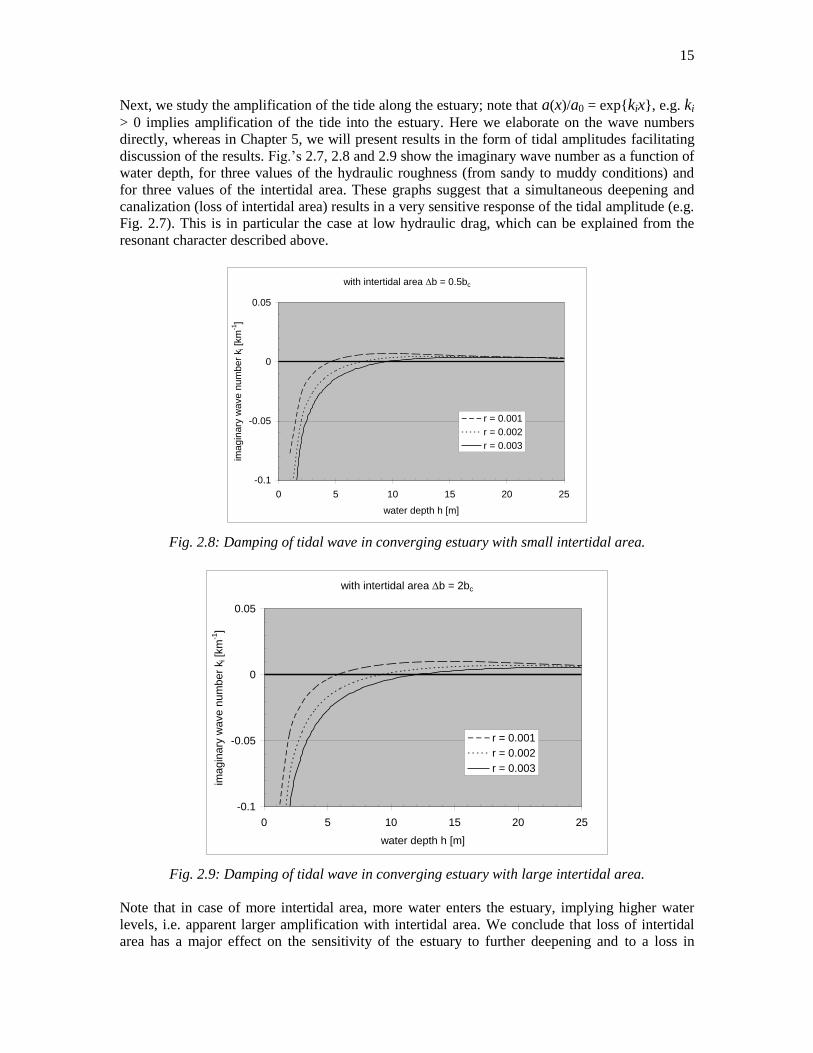
Next, we study the amplification of the tide along the estuary; note that a(x)/a0 = exp{kix}, e.g. ki

> 0 implies amplification of the tide into the estuary. Here we elaborate on the wave numbers

directly, whereas in Chapter 5, we will present results in the form of tidal amplitudes facilitating

discussion of the results. Fig.’s 2.7, 2.8 and 2.9 show the imaginary wave number as a function of

water depth, for three values of the hydraulic roughness (from sandy to muddy conditions) and

for three values of the intertidal area. These graphs suggest that a simultaneous deepening and

canalization (loss of intertidal area) results in a very sensitive response of the tidal amplitude (e.g.

Fig. 2.7). This is in particular the case at low hydraulic drag, which can be explained from the

resonant character described above.

with intertidal area b = 0.5bc

-0.1

-0.05

0

0.05

0 5 10 15 20 25

water depth h [m]

ima

gin

ary

wa

ve

nu

mb

er

k i [

km

-1]

r = 0.001

r = 0.002

r = 0.003

Fig. 2.8: Damping of tidal wave in converging estuary with small intertidal area.

with intertidal area b = 2bc

-0.1

-0.05

0

0.05

0 5 10 15 20 25

water depth h [m]

imagin

ary

wave n

um

ber

k i [

km

-1]

r = 0.001

r = 0.002

r = 0.003

Fig. 2.9: Damping of tidal wave in converging estuary with large intertidal area.

Note that in case of more intertidal area, more water enters the estuary, implying higher water

levels, i.e. apparent larger amplification with intertidal area. We conclude that loss of intertidal

area has a major effect on the sensitivity of the estuary to further deepening and to a loss in

16

overall hydraulic drag. One may conclude that the resilience of the estuary to human interferences

reduces rapidly with the loss of intertidal area.

no intertidal area b = 0, a = 0.5 m

1

1.2

1.4

1.6

1.8

2

0 5 10 15 20 25

water depth h [m]

tid

al a

sym

me

try

r = 0.001

r = 0.002

r = 0.003

flood dominant

no intertidal area b = 0, a = 1.0 m

1

1.2

1.4

1.6

1.8

2

0 5 10 15 20 25

water depth h [m]

tid

al a

sym

me

try

r = 0.001

r = 0.002

r = 0.003

flood dominant

Fig. 2.10: Tidal asymmetry HW LWc c without intertidal area.

with intertidal area b = 0.5bc, a = 0.5 m

0.5

0.75

1

1.25

1.5

1.75

2

0 5 10 15 20 25

water depth h [m]

tid

al a

sym

me

try

r = 0.001

r = 0.002

r = 0.003

flood dominant

ebb dominant

with intertidal area b = 0.5bc, a = 1.0 m

0.5

0.75

1

1.25

1.5

1.75

2

0 5 10 15 20 25

water depth h [m]

tid

al a

sym

me

try

r = 0.001

r = 0.002

r = 0.003

flood dominant

ebb dominant

Fig. 2.11: Tidal asymmetry HW LWc c with some intertidal area.

with intertidal area b = 2bc, a = 0.5 m

0

0.5

1

1.5

2

0 5 10 15 20 25

water depth h [m]

tid

al a

sym

me

try

r = 0.001

r = 0.002

r = 0.003

flood dominant

ebb dominant

with intertidal area b = 2bc, a = 1.0 m

0

0.5

1

1.5

2

0 5 10 15 20 25

water depth h [m]

tid

al a

sym

me

try

r = 0.001

r = 0.002

r = 0.003

flood dominant

ebb dominant

Fig. 2.12: Tidal asymmetry HW LWc c with large intertidal area.

Our linear analysis also allows for an assessment of tidal asymmetry, analyzing the celerity at

high and low water, e.g. equ. (20). This analysis requires information on the tidal amplitude, and

we present results for a = 0.5 m and a = 1 m (kept constant along the river), bearing in mind that

17

the amplitude should be small compared to water depth in our linear approach. The tidal

asymmetry parameter is presented in the Fig.’s 2.10, 2.11 and 2.12 as a function of water depth

for three values of hydraulic drag and three values of intertidal area. Remember that > 1 implies

flood dominant conditions.

These graphs suggest a large sensitivity of the tidal asymmetry as a function of the size of the

intertidal area. Without intertidal area, the estuary is always flood dominant. This dominance

decreases with increasing depth and roughness, but is shown to increase rapidly with tidal

amplitude. Small areas of intertidal area (represented by b = 0.5bc) already have a major effect

on the tidal asymmetry. However, Fig. 2.11 suggests that with increasing amplitude such

transition can be obtained at larger depths only. Or, in other words, after deepening, restoration of

the intertidal only is likely not sufficient to restore the original situation.

These results further suggest that in very shallow estuaries, with depths of a few meters only,

flood dominant conditions will always prevail, even for very large intertidal areas.

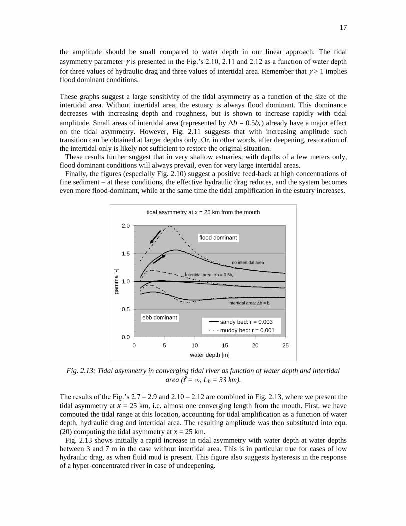
Finally, the figures (especially Fig. 2.10) suggest a positive feed-back at high concentrations of

fine sediment – at these conditions, the effective hydraulic drag reduces, and the system becomes

even more flood-dominant, while at the same time the tidal amplification in the estuary increases.

tidal asymmetry at x = 25 km from the mouth

0.0

0.5

1.0

1.5

2.0

0 5 10 15 20 25

water depth [m]

ga

mm

a [-]

sandy bed: r = 0.003

muddy bed: r = 0.001

no intertidal area

intertidal area: b = 0.5bc

flood dominant

ebb dominant

intertidal area: b = bc

Fig. 2.13: Tidal asymmetry in converging tidal river as function of water depth and intertidal

area (ℓ = , Lb = 33 km).

The results of the Fig.’s 2.7 – 2.9 and 2.10 – 2.12 are combined in Fig. 2.13, where we present the

tidal asymmetry at x = 25 km, i.e. almost one converging length from the mouth. First, we have

computed the tidal range at this location, accounting for tidal amplification as a function of water

depth, hydraulic drag and intertidal area. The resulting amplitude was then substituted into equ.

(20) computing the tidal asymmetry at x = 25 km.

Fig. 2.13 shows initially a rapid increase in tidal asymmetry with water depth at water depths

between 3 and 7 m in the case without intertidal area. This is in particular true for cases of low

hydraulic drag, as when fluid mud is present. This figure also suggests hysteresis in the response

of a hyper-concentrated river in case of undeepening.

18

For the case with some intertidal area (b = 0.5bc) the tide is more or less symmetrical, except

at low hydraulic drag. When the intertidal area is sufficiently large, ebb-dominant conditions

always prevail, and the river is fairly resilient to deepening, as no feed-back occurs.

Fig. 2.13 suggests that in case of no or little intertidal area, deepening leads to progressive flood-

dominant conditions, pumping mud into the estuary (or arresting river-borne sediments), as a

result of which the hydraulic drag decreases and asymmetry increases further. This would yield a

hysteresis in the response of the river to deepening – re-establishing the initial depth will not

automatically lead to the pre-deepening conditions of the river.

19

3. Fine sediment transport in narrow estuaries

3.1 Transport components

In the previous section, we have discussed the development of the tide in a converging estuary.

However, an assessment of the tidal evolution of the dynamics of fine sediment transport requires

more information. In this section we derive the components for the transport of fine sediment in

narrow estuaries, i.e. lateral gradients are small, an discuss components are affected by the tidal

dynamics discussed in Chapter 2. We follow Uncles (1985), Fischer et al. (1979) and many others

in the decomposition of fine sediments in narrow estuaries. The cross section of the estuary is

schematized as before through the compound channel in Fig. 2.1, and we neglect all lateral

variations in the flow-carrying cross section. Moreover, again we assume that the flow-carrying

cross section Ac may be modeled as c cA hb . The longitudinal transport of fine sediment is

described with the advection-diffusion equation, in which the effects of exchange of fine

sediment between main channel and intertidal area, and over the cross-section of the estuary are

accounted for by a dispersion term Dx:

, ,

c cc x c

b b hc b huc chb D P x t S x t b b

t x x x

(22a)

in which huc is the fine sediment flux f(x,t) per unit width through the flow-carrying cross

section, and P and S are production (f.i. from erosion) and sink terms (in particular sedimentation

on intertidal areas) per unit width. In the case of a dynamic equilibrium, we may cancel erosion

and deposition in the channel itself, and only the sink term in (22a) is maintained. If we further

neglect longitudinal turbulent diffusion, we can simplify equ. (22a) into

1

,c c

c c b c

b bhc huc bhuc S x t

t b b x b b L b b

or

(22b)

,c

c b c

bhc f f bS x t

t b b x L b b

(22c)

Further to its effects on the tidal movement in a converging estuary, the loss of intertidal area will

reduce accommodation for deposition of fine sediment (S 0), and the mass of sediment in the

estuary per unit width hc increases.

Next, we elaborate on the flux f addressing the various contributions by estuarine circulation,

tidal asymmetry, etc. Therefore, water depth h, flow velocity u and suspended sediment

concentration c are decomposed in depth-mean values, their variation over depth, tide-mean

values, and variation over time2)

:

2)

Note that in our schematization bc and b are not a function of time, though at low water, btot = bc.

20

with

,

,

1 1d 0, d 0

T h

h h h t

u u u t u z u z t

c c c t c z c z t

x x t x zT h

x

(23)

in which and represent variation over time and depth, respectively, and triangular brackets

and overbar averaging over the tidal period T and water depth h, respectively. Note that all

parameters in equ. (23) are still a function of x. Substituting equ. (23) into the advection term of

equ. (22a), yields for the longitudinal sediment flux per unit width F [kg/m], integrated over the

depth first and next over the tidal period:

d d

T h

r S p a g

F uc z t T f T huc

T h u c h u c h u c h u c

h u c u c u c u c u c u c u c

T u h c h u c h u c

h u c h u c h u c h u c F F F F F

v lF F

(24)

Here we have defined the following six contributions to the longitudinal transport of fine

sediment, ignoring the possible longitudinal transport by dispersion (Dx; even though this

transport can be large):

Fr Residual fine sediment transport as a result of net river flow and a net transport rectifying

for Stokes drift, in which u = residual flow velocity (river flow and rectifying Stokes

drift). If the Stokes drift is zero, as for low-friction synchronous converging (short)

estuaries, then r rivF Tq h c h , where qriv = specific river discharge, i.e. per unit

width.

FS This term is known as the Stokes drift. For a low-friction synchronous(short) estuary with

exponentially converging river plan form. For fine sediments, which are reasonably well

mixed over the water column, the Stokes drift Fs and its rectification are more or less

equal, and we do not further discuss these terms.

Fp This term is generally known as tidal pumping. Note that this term represents the

important asymmetries in peak velocity and in slack water velocity (scour and settling

lag), and is responsible for the net transport of (fine) sediment by tidal asymmetry. We

21

will therefore refer to this term as Fa, highlighting the tidal asymmetry contributions. The

tidal analysis discussed in Chapter 2 focuses on this term.

Fg This term is generally referred to as the estuarine circulation, or gravitational circulation,

induced by longitudinal salinity gradients – sometimes longitudinal gradients in

temperature and/or suspended sediment may play a role as well, but these are not

elaborated in this report.

Fv This term represents asymmetries in vertical mixing, sometimes referred to as internal

tidal asymmetry (Jay and Musiak, 1996). Note that these asymmetries can be induced by

vertical salinity gradients, and/or by vertical gradients in suspended sediment.

Fl The last two terms are triple correlations, and represent lag effects, such as around slack

water, and settling and scour lag (e.g. Dronkers, 1986; Postma, 1961; and Van Straaten &

Kuenen, 1957 & 1958). Note that these triple products are often ignored in literature on

the decomposition of transport fluxes, though they can be very important, in particular for

starved-bed conditions.

The decomposition of transport terms was first developed to study the salinity distribution in

estuaries (e.g. Dyer, 1997 and Fischer et al., 1979). Later, for instance Uncles (1985) and others

applied this technique analyzing sediment fluxes in estuaries. Note that different authors use

various definitions for the transport components in equ. (24) – the various terms therefore may

not always directly be compared with literature values.

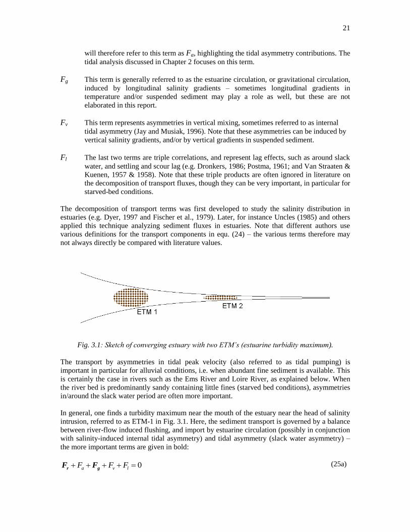
Fig. 3.1: Sketch of converging estuary with two ETM’s (estuarine turbidity maximum).

The transport by asymmetries in tidal peak velocity (also referred to as tidal pumping) is

important in particular for alluvial conditions, i.e. when abundant fine sediment is available. This

is certainly the case in rivers such as the Ems River and Loire River, as explained below. When

the river bed is predominantly sandy containing little fines (starved bed conditions), asymmetries

in/around the slack water period are often more important.

In general, one finds a turbidity maximum near the mouth of the estuary near the head of salinity

intrusion, referred to as ETM-1 in Fig. 3.1. Here, the sediment transport is governed by a balance

between river-flow induced flushing, and import by estuarine circulation (possibly in conjunction

with salinity-induced internal tidal asymmetry) and tidal asymmetry (slack water asymmetry) –

the more important terms are given in bold:

0a v lF F F r gF F (25a)

22

It may be argued that as long as the river flow is large enough to flush the turbidity maximum out

of the river at times (once a year?), no fine sediments can accumulate in the river forming hyper-

concentrated conditions. Our linear model is unsuitable to analyze such conditions in more detail,

though a qualitative description is given in Section 3.2.

When suspended sediment concentrations within the river, and/or when sediment loads from the

river are large, a second turbidity maximum may be formed (ETM2 in Fig. 3.1) through a balance

by river-induced flushing and tidal asymmetry (peak velocities and internal asymmetry):

0v lF F r aF F (25b)

Again, the most important processes are given in bold. Such a second ETM is found for instance

in the Ems River (Fig. 3.2) where high suspended sediment concentrations are found in the fresh

water region, well beyond the head of salinity intrusion. However, Fig. 3.2 suggests that within

the Ems no localized ETM is found, but a large patch of highly turbid water that moves to and

from with the tidal excursion. We anticipate that this is due to the slow remobilization of

sediment from the bed, inducing a longitudinal dispersion of the sediment over the tidal

excursion.

Fig. 3.2: Measured (August 2, 2006) salinity and SPM distributions in the Ems River during flood

and ebb (after Talke et al., 2009) – note that the suspended sediment dynamics have become

independent of the salinity dynamics.

In Section 3.4 we describe qualitatively the evolution from a “normal” estuary to a hyper-

concentrated system, with the Ems River as an example. We argue that it is the change in

dominant processes, e.g. from the balance of equ. (25a) to (25b) which characterizes this regime

shift, and which is responsible for the persistence of this new regime with its second turbidity

maximum (ETM 2).

23

3.2 Reduction in effective hydraulic drag

In Chapter 2 we have shown that the response of the tide in a converging estuary is sensitive to

the effective hydraulic drag. In this section we present a simple formula to assess reductions in

hydraulic drag as a function of suspended sediment concentration. Note that these formulae do

not apply for very high concentrations, when fluid mud is formed (occasionally).

Winterwerp et al. (2009) derived a simple formula to quantify the reduction in hydraulic drag as a

function of enhanced levels of suspended sediment concentration and longitudinal salinity

gradients:

0 0*

*

4eff SPM

ref

C C C Cu h

u hg g g g Ri

(26a)

or in terms of excess Chézy coefficient:

*4effC

hg

Ri

(26b)

in which the Rouse number and bulk Richardson number *Ri are defined as:

* 2 2

* **

and b w T s

b w

cghgh W

u uc u

Ri

(27)

0

10

20

30

40

50

0 0.1 0.2 0.3 0.4

Ri*

C/g

0.5

h = 1 m

h = 5 m

h = 10 m

h = 20 m

Fig. 3.3: Effective hydraulic drag (Chézy coefficient) as function of the bulk Richardson and

Rouse number.

From the implicit equ. (27) we can draw the following conclusions on the effective Chézy

number:

1. The effective Chézy coefficient increases, hence the hydraulic drag decreases with

increasing water depth.

24

2. The effective Chézy coefficient increases with suspended sediment concentration c.

3. The effective Chézy coefficient increases with settling velocity, hence with flocculation.

Note that the reduction in effective hydraulic drag is essentially induced by vertical stratification,

induced by vertical gradients in the suspended sediment (SPM) concentration. Because of

hindered settling effects, the same vertical gradient in SPM concentration can exist at relatively

low and relatively high concentrations. Or in other words, low- and high-concentrated mixtures

can be kept in suspension with the same kinetic energy (e.g. Section 3.3).

Hence, the effective Chézy coefficient scales with the following dimensionless parameters:

*,effC

g Ri

(28)

The relation between the effective Chézy coefficient and suspended sediment concentrations (e.g.

equ. (26)) is shown in Fig. 3.3. Note that the rivers discussed in this report have water depth of

typically 5 – 10 m, hence we expect an increase in the effective Chézy coefficient by 15 – 30

m1/2/s. Only the Elbe is considerably deeper, and the excess Chézy value is therefore expected to

be larger as well.

3.3 Hyper-concentrated conditions

The literature contains a variety of definitions on hyper-concentrated conditions. In this section,

we present a definition which is relevant for the present study. Winterwerp (2011) argues that the

Ems and Loire River are currently in these hyper-concentrated conditions.

In our definition, hyper-concentrated conditions are related to the concept of saturation (e.g.

Winterwerp, 2001). Let us assume a straight, prismatic channel with a uniform flow at flow

velocity U1. First, we analyze the transport of sand in suspension. From all classical literature,

and data on sand transport, we know that an equilibrium sand transport is established, with an

equilibrium vertical profile in suspended sand concentration, which can be described with a

classical Rouse profile. This profile describes a balance between vertical turbulent mixing and

settling of the grains by gravity. If the flow velocity U1 is reduced to U2, then a new equilibrium

is established immediately, at smaller suspended sand concentrations though. A new equilibrium

between vertical turbulent mixing and settling is established, the suspended sand concentration

being smaller because turbulent mixing is smaller owing to the decrease in flow velocity. Note

that upon deposition from state 1, sand grains form a rigid bed immediately, allowing full

turbulent production, at state 2 conditions, though.

In the case of fine suspended sediment, a different picture emerges, owing to the fact that fine

sediment consists of flocs with high water content (up to 95%). When the flow velocity decreases

from U1 to U2, the fine sediment flocs settle as well, owing to the decrease in turbulent mixing in

response to the lower flow velocity. However, these flocs do not form a rigid bed immediately,

but a layer of soft fluffy sediment. As a result, turbulence production decrease beyond the value

expected at state 2 conditions over a rigid bottom, and more flocs settle, as turbulent mixing drops

further. This snowball effect continues till virtually all flocs have settled on the bed: a layer of

fluid mud has been formed. These conditions are referred to as saturation, and have been

elaborated in detail in Winterwerp (2001).

25

A similar condition emerges when the flow velocity is kept constant, but the suspended fine

sediment concentration slowly increases. At a certain level, referred to as the saturation

concentration, vertical turbulent mixing is too small to keep the flocs in suspension, and a fluid

mud layer is formed by the snowball effect described above. This is depicted in Fig. 3.4 (e.g.

Winterwerp, 2011, 2006). The horizontal axis depicts the volumetric concentration of the

suspended sediment, in case of fine sediment, the volume concentration of the flocs; the vertical

axis depicts the flux Richardson number Rif, a parameter describing that part of the kinetic

energy of the flow available for mixing.

0

0 0.2 0.4 0.6 0.8 1

volumetric concentration f

flu

x R

ich

ard

so

n n

um

be

r R

i f

super-saturated conditions

low/high-conc. sub-sat. suspension

hyper-conc. sub-sat. suspension

Ricr

U1

U2; U2 < U1

low-conc. susp.

high-conc.

susp.

Ems & Loire conditions

Fig. 3.4: Stability diagram showing saturation and super-saturated conditions (dotted line). At

smaller concentrations rivers are in the left branch of the diagram, at higher concentrations,

right-branch conditions prevail – these are referred to as hyper-concentrated conditions. The flux

Richardson number Rif yields a proxi for the (kinetic) energy required for vertical mixing, and

this diagram shows that each value of Rif (at sub-critical conditions) can be obtained with two

different volumetric concentrations.

From the above, and from Fig. 3.4 we can conclude that at low suspended sediment

concentrations (left branch of Fig. 3.4), an increase in suspended sediment concentration, for

instance through erosion of the bed, will ultimately lead to a collapse of the concentration profile,

the formation of fluid mud, hence super-saturated conditions. In terms of Fig. 3.4, we follow the

stability curve to the right, and up to larger Rif values until a critical value is surpassed. In

Section 3.2 we have shown that prior to these conditions, already a profound decrease in effective

hydraulic drag may occur.

In the right-hand branch of the stability diagram, we refer to hyper-concentrated conditions. The

suspended sediment concentration is so high, that the sediment’s settling velocity decreases

significantly (up to two orders of magnitude), so that very little turbulent energy/mixing is

required to keep the sediment in suspension. Furthermore, we note that if the flow would erode

sediment from the bed, we would follow the stability curve to the right, but now to lower Rif values, contrary to the low-concentrated conditions above. This implies that the suspension

becomes more stable: “it likes” to erode the bed, reducing the energy to keep the sediment in

suspension. This is one reason that hyper-concentrated conditions are so persistent, and that

rivers, such as the Ems and the Loire, brought into these hyper-concentrated conditions, are

26

difficult to train back into conditions more favorable from an environmental point of view. The

reader is referred to Bruens et al. (2012) for a full analysis on the stability of these hyper-

concentrated conditions, and why they do not consolidate, but remain fluid over such long periods

of time.

3.4 A qualitative description of the regime shift in the Ems estuary

Winterwerp (2010) analyzed how the Ems River responded to ongoing deepening. We have no

data on the transition of the Ems River from a “normal” turbid river into its current, hyper-

concentrated state over time (Fig. 3.2). Therefore, we have developed a conceptual picture for the

transition of the river as a result of deepening from its former equilibrium, using our observations

described on the previous pages. This picture is summarized in Table 3.1. We start a long time

ago from a long-term equilibrium, referred to as phase 0 in Table 3.1, at which up-river directed

fine sediment transport induced by gravitational circulation and the various effects of tidal

asymmetry balance the down-river transport induced by the river flow. The fine sediments in the

Ems River are mainly marine-born, though some sediment may be delivered by the river. Over

shorter time periods, accumulation or flushing may occur, as a result of e.g. varying river flows.

Under these conditions, the formation of an estuarine turbidity maximum (ETM) is expected near

the head of the saline intrusion. Over longer time scales, land formation initiated on vegetated

mudflats, may reduce the river’s tidal volume, affecting the long-term morphodynamic

equilibrium.

As a response to deepening, net accumulation is expected, restoring equilibrium, Phase 1, Table

3.1. The underlying processes are a decrease in river-induced flushing, as river flow velocities

decrease in proportion to the river’s cross section, in conjunction with an augmented net transport

by gravitational circulation, as water depth increase (scales with h2). Deepening would also

increase tidal asymmetry in case of reduced intertidal areas (e.g. Chapter 2). Possibly, reduced

vertical mixing already starts to play a role, enhancing the trapping efficiency of the river (see

below). As the accumulating fine sediments do not form a rigid bed immediately, also turbidity

levels increase, as more sediments are available for remobilization, and suspended sediment

concentrations in the ETM increase.

A further increase of the river’s depth would increase the amount of remobilizable sediments

further, accompanied by a further increase in suspended sediment concentrations. When the

riverbed becomes predominantly muddy, profound feed-backs between the various processes are

expected through which the river evolves into its present hyper-concentrated state. In this regime,

gravitational circulation still plays a role, but its effect is small compared to the dominant

contributions of internal tidal asymmetry, with profound differences in vertical mixing during ebb

and flood: during ebb, the river is highly stratified by sediment-induced buoyancy destruction.

Winterwerp (2010) suggests that this regime shift may be initiated in the Ems River at depth-

averaged concentrations typically of the order of a few 100 mg/l. Then, the trapping efficiency of

the river increases rapidly as a result of vertical stratification during ebb, and asymmetry in floc

size. The rate at which the river really accumulates fine sediments is determined merely by the

supply of these sediments from the Wadden Sea – Dollard estuary, than by internal hydro-

sedimentological processes.

We anticipate a second regime shift in the estuary, Phase 3, Table 3.1, when the river starts to

develop pronounced occurrences of fluid mud, as observed presently by Schrottke (2008). In that

case, fine sediment transport rates are expected to be dominated by the tidal asymmetry of the

27

peak currents themselves. Now re-entrainment of the fluid mud layers, which scales with U3 as

well, becomes a dominant mechanism (Bruens et al., 2012). Sediment is transported up-river

towards the river’s head at Herbrum by the large tidal asymmetry, and the entire river becomes

highly turbid. As the consolidation rate of fluid mud layers scales with their thickness squared,

we expect that the properties of the fluid mud layer are fully determined by the velocities during

flood conditions. Note that not much consolidation of the thick fluid mud layers during ebb is

expected.

Table 3.1: Summary of Ems River response to its deepening – see text for further explanation;

river depth in Phases 2 and 3 are not necessarily larger than in Phase 1. Phase 0 refers to

“undisturbed” state of the river.

phase dominant transport processes comments

flood-directed transport ebb directed transport

0 “normal” estuary with ETM; equilibrium†)

long-term

balance between

ebb and flood

transport

(slack water) tidal asymmetry; river-induced flushing

gravitational circulation)

1 small disturbance; transient state net import;

(slack water) tidal asymmetry ? reduced river-induced flushing weak feed back

enhanced gravitational circ.

2 large disturbance; transient state large net import;

internal tidal asymmetry: mixing & floc size; strong feed-back;

limited sediment load & determined by ebb conditions; large trapping

fairly well-mixed flood; stratified ebb;

relative unimportant grav. circ.;

sediment-induced grav. circ. ?

fluid mud;

small ebb transport

3 hyper-concentrated estuary; new equilibrium‡)

large net import;

asymmetry in tidal velocity; strong feed-back;

internal tidal asymmetry; large trapping

pronounced fluid mud formation;

capacity conditions; transport formula applicable

) Including possible effects of internal asymmetry, in particular when the salinity field is stratified,

†) Long-term equilibrium may be disturbed by land formation, reducing estuary’s tidal volume,

‡) Without maintenance, estuary may return towards its original state if a rigid bed can be formed.

In summary, we infer that in response to deepening of the Ems River, the sediment load in the

river first increases through an increase in the up-river transport by gravitational circulation and a

decrease in river-induced flushing. Then, in the second phase of the river’s transition towards its

hyper-concentrated state, when the concentration in the river attains values of a few 100 mg/l,

internal tidal asymmetry becomes dominant because of pronounced interactions between the

sediment load, and the turbulent water movement and vertical mixing. We believe that the 1990-

survey conditions (e.g. Van Leussen, 1994) fall within this second phase of development. Finally,

the load of fine sediment becomes so large that in the final phase of the river’s evolution, thick

fluid mud layers are formed, and the up-river fine sediment transport is dominated by tidal

28

asymmetry of the current velocity. The second phase in transition is probably not stable: trapping

is so large that a further development towards the final phase may be inevitable; the time scale of

this intermediate phase depends mainly on the sediment supply, and may amount to a decade or

so, as in the Ems River.

Finally, tidal reflections from the weir at Herbrum are expected to augment the tidal range by a

few dm (e.g. Fig. 2.4), further increasing the tidal pumping of mud into the river.

29

4. Comparison of various estuaries

In this section, we compare properties and evolution of a number of estuaries and tidal rivers:

Ems – Germany & The Netherlands

Loire – France

Elbe – Germany

Weser – Germany

Upper Sea Scheldt – Belgium

We have some data available for the Humber (Ouse) and Tamar, both in the UK, the Garonne and

Vilaine, both in France, and the Passaic River in the USA. Note that Kuijper presented similar

analyses for the Western Scheldt estuary.

In the following, the data of the various rivers are analyzed – a synthesis of this analysis is given

in Chapter 5. In this phase of the study we ignore the effects of reflection by a weir, as this is not

easily to be accounted for in an analytical approach. Based on the graphs of Fig. 2.4, it is

anticipated that the tidal amplitude is under-estimated with the single-wave analytical model by a

few decimeter. This implies that a lower friction coefficient (larger Chézy value) is required in

calibrating the model to reproduce observed tidal elevations. However, we expect that the relative

effect of deepening and fine sediments are still reasonably well predicted.

In a next phase of the study we will account for the effects of reflections on barriers/weirs in the

river, but the in current study we discuss the effects of reflections only qualitatively.

The procedure of our data analysis is as follows:

1. We determine the convergence length Lb of the estuary, and its possible variations over

time, by plotting the width of the river against its longitudinal co-ordinate.

2. We establish historical variations in (mean) water depth and intertidal area, and compute

(variations) in the estuarine convergence number e.

3. We compute the imaginary wave number ki between subsequent tidal stations from its

definition 2 1 2 1exp ia a x x k , where a2 = tidal amplitude at x = x2 (etc.), and

make ki dimensionless with Lb.

4. We plot the resulting values of i against e, yielding one data point for each river stretch

in a certain time period.

5. We then fit the analytical model (equ.’s (11)) through the data by tuning the roughness

parameter r*. Note that we assume an infinite long river, but sub-divide the river in sub-

sections with more or less constant water depth.

6. We determine the effective Chézy coefficient C from the fitted *r -values. For this we use

the solution for u from the analytical model (e.g. equ. (41) and (5c)).

7. We plot the variation of C with time identifying possible changes in effective hydraulic

drag over time.

Hence, the linear model discussed in Chapter 2 is merely used as a tool to analyze the historical

data from the various rivers. By making tidal amplification/damping and river

geometry/bathymetry dimensionless, we can compare the various rivers mutually (e.g. Chapter

5).

30

4.1 The Ems River

The Ems River is about 53 km long from the weir at Herbrum to Emden, flowing through

Germany into the Ems-Dollard estuary (Fig. 4.1). This river is renowned for its large suspended

sediment concentrations, with values up to 30 – 40 g/l over most of the upper part of the river

(e.g. Talke et al., 2009). These high concentrations are found well beyond the region of salinity

intrusion, and move to and fro with the tide. Also profound layers of fluid mud are found, in

particular around slack water and neap tide (e.g. Schrottke, 2008). Currently, the total mass of

suspended solids amounts to about 1 Mton, while yearly about 1.5 Mton of solids is removed

from the Ems River by dredging. For further details on the river, the reader is referred to Krebs

and Weilbeer (2005).

The Ems River is characterized by a profound tapering, as shown in Fig. 4.2. The overall

convergence length of the river amounts to about 19 km, whereas for the stretches between

Emden – Leeroort Lb ≈ 32 km, Leeroort – Papenburg Lb ≈ 27 km, and Papenburg – Herbrum Lb ≈

33 km. In the following, we refer to these three sections as E-L, L-P and P-H. The apparent

discrepancy of the overall convergence length and those of three smaller stretches of the river is

attributed to some jig-saw patterns in the b-x curve (e.g. Fig. 4.2). In our analysis, we used the

larger values.

Fig. 4.1: Lay-out of Ems-Dollart estuary and Ems River.

An overview of the various interventions in the river was summarized in Vroom et al. (2012),

based on information from Rijkswaterstaat and the Bundesanstalt fur Wasserbau. The evolution

in depths of the river for the three stretches E-L, L-P and P-H is presented in Fig. 4.3, where the

depths have been averaged to obtain mean values for these stretches. Note that after 1940 no

reclamation of intertidal area took place, though we anticipate that a large part of the remaining

31

intertidal areas has been lost in due time owing to sedimentation on these areas (see discussion

below). Around 1961, in the upper part of the river (P-H), groins have been constructed,

narrowing the river locally.

convergence length Ems RIver

y = 931.74e-5E-05x

10

100

1000

0 10000 20000 30000 40000 50000 60000

length w.r.t. Emden [m]

wid

th b

c [

m]

Le

ero

ort

Pa

pe

nb

urg

He

rbru

m

Lb = 19 km

Fig. 4.2: Convergence length of Ems River.

The response of the tidal range to these interventions is presented in Fig. 4.4, in conjunction with

an overview of the human interventions (Herrling, 2007). Fig. 4.4 suggests that the response of

the tidal range to the various interventions is not instantaneous, but takes considerable time to

attain equilibrium – Fig. 4.4 suggests a time scale of at least 20 years. We will address this further

below. Finally, it is noted that the tidal range at Herbrum becomes highly irregular as a result of

variations in the yearly river flow – this will be elaborated in another study.

evolution of water depths Ems River

2

4

6

8

10

1940 1960 1980 2000 2020

year

de

pth

w.r

.t.

MS

L [

m]

Emden - Leeroort

Leeroort - Papenburg

Papenburg - Herbrum

Fig. 4.3: Evolution of mean water depths in Ems River for three trajectories (water depth with

respect to mean sea level at Emden).

32

We note that more regular data are to be expected from harmonic analyses, including the effects

of the 18.6 year cycle (see also Chapter 4.5 on the Scheldt data). However, the original data are

not in our possession.

tidal evolution Ems River

0

1

2

3

4

1920 1940 1960 1980 2000 2020

year

tid

al ra

ng

e [

m]

km 0: Emden

km 25: Leeroort

km 40: Papenburg

km 53: Herbrum

4.5-4/4-4.5 m 5.5/4.1 m 5.5/5 m 5.7 m

narrowing

7.3 m

6.8 m

6.5 m

Fig. 4.4: Evolution of measured mean tidal range in Ems River and summary of interventions –

5.5/4.1 m indicates a design depth of 5.5. m over the Emden-Leeroort reach, and 4.5 m over the

Leeroort-Papenburg reach; Design depth Papenburg-Herbum reach was 3 m till 1980, and then

3.5 m (data from BAW, and prior to 1950 by Herrling, 2007).

evolution amplification Ems River

-0.04

-0.03

-0.02

-0.01

0

0.01

1940 1960 1980 2000 2020

year

ki [k

m-1

]

Emden - Leeroort

Leeroort - Papenburg

Papenburg - Herbrum

Fig. 4.5: Evolution of imaginary wave number in Ems River; note that in the remainder the data

for the trajectory Papenburg – Herbrum have been ignored because of their irregularity.

33

evolution dimensionless damping

-1.5

-1.0

-0.5

0.0

0.5

0.0 0.5 1.0 1.5 2.0

convergence parameter e [-]

im.

wa

ve

nu

mb

er

[-]

Emden - Leeroort

Leeroort - Papenburg

Fig. 4.6: Evolution of dimensionless imaginary wave number i with variations in estuarine

convergence number e.

From Fig. 4.4, the imaginary wave number ki (amplification factor) was determined. For this

purpose, mean values over a period of five subsequent years were determined from the Fig. 4.4-

data, and then ki was determined by dividing the tidal range at Leeroort by that at Emden, etc.

The results are presented in Fig. 4.5, showing a regular increase in ki for the trajectories E-L and

L-P. However, for the trajectory P-H, a highly irregular behavior is found. The pattern of this

behavior can be entirely changed by using another averaging procedure for the data of Fig. 4.4, or

using the tops or troughs of the curve. At present, we are not sure which behavior is

representative, and we therefore ignore the behavior of the tide along the trajectory Papenburg –

Herbrum. We believe that only a detailed harmonic analysis of the tidal measurements (M2

component) can shed light on the irregular behavior of the Herbrum tidal curve.

Finally it is noted that for both trajectories E-L and L-P the data show that amplification of the

tide is observed from 1995 on – before the tidal wave was still damped, though little only.

Next, the imaginary wave number is made dimensionless by the convergence length Lb (e.g. i ,

equ. 8 & 11) and plotted against the estuarine convergence number e in Fig. 4.6. Then the linear

solution (equ. 13b) is fitted to the data by tuning the roughness parameter *r , appreciating that the

assumptions to attain this linear solution are grossly violated (in particular the tidal range is not

small compared to the water depth, and the water depth itself is not constant along the two

trajectories under analyses. Yet, the linear solution should allow us to analyze the trends in the

data observed in the Ems River.

The results of the calibration are shown in Fig. 4.7, in which the data, presented before in Fig. 4.6

have now been colored to mark the various intervention periods in the river. The 1960 data and

earlier for L-P can be fitted with *r = 7, whereas the 1980 data require *r = 4. Note that

interventions were carried out in 1960 and 1983 – the response to the 1960 intervention was

apparently not yet at equilibrium in 1980.

34

evolution dimensionless damping

-1.5

-1.0

-0.5

0.0

0.5

0.0 0.5 1.0 1.5 2.0

convergence parameter e [-]

im.

wa

ve

nu

mb

er

[-]

Emden - Leeroort

Leeroort - Papenburg

< 1960

1960 - 1980

1985 - 1995

> 1995 r* = 7

r* =4r* =3.3

r* = 2.5

r* = 1.7

Fig. 4.7: Fits of linear solution to observed data through tuning of roughness parameter in i –

e diagram.

For a more physical interpretation, the roughness parameter *r has to be converted; arbitrarily we

choose to convert to the Chézy coefficient C. In this conversion we use the observed water depth

for the various years, and use the imaginary wave number ki to determine the flow velocity along

the river, assuming that in the 1960s, the peak velocity at Emden was 1 m/s (e.g. equ. 4a). To

obtain the variation of C with time, we have fitted the linear solution (as in Fig. 4.7) through all

data points by tuning *r , the results of which are presented in Fig. 4.8.

evolution of effective hydraulic drag Ems River

0

20

40

60

80

100

1940 1960 1980 2000 2020

year

Ch

ezy

[m

1/2

/s]

Emden - Leeroort

Leeroort - Papenburg

Fig. 4.8: Evolution of effective hydraulic drag (Chézy coefficient) with time.

Fig. 4.8 suggests that up to the 1960s the Ems River was quite rough, with Chézy values in the E-

L reach of about 60 m1/2

/s, which is typical for a sandy river bed. Further upstream, in the L-P

reach, Chézy values as low as 40 m1/2

/s are found. We are not certain that these are correct, but if

so, they may be indicative for profound steep bed forms (dunes), such as observed for instance in

the Elbe and Weser Rivers (e.g. Van Rijn, 1993). The gradual increase in Chézy coefficient

between the 1960s and 1980s may then be attributed to a gradual decrease in dune heights and

steepness owing to ongoing dredging. However, from the 1990’s onward, the Ems River became

35

more and more infamous for its very high suspended sediment concentrations with hyper-

concentrated values after 2000. Today, suspended sediment concentrations measure several 10

g/l, e.g. Talke et al. (2009). The very large values of C = 80 – 90 m1/2

/s can be explained by the

profound buoyancy-induced damping by the large suspended sediment concentrations. Note that

Fig. 4.8 suggests an increase in Chézy values of 15 – 25 m1/2

/s for the conditions prevailing in the

Ems River with water depths between 5 and 10 m.

As we have ignored the effects of tidal reflections against the weir at Herbrum we expect that the

Chézy values, in particular for the trajectory Leeroort-Papenburg (e.g. Fig. 2.4) are a bit over-

estimated, and should be lower by a value of 5 – 10 m1/2

/s.

Fig. 4.9: Measured travel time tidal wave along Ems River (Herrling, 2007).

travel time tidal wave

0

0.5

1

1.5

0 0.5 1 1.5

measured [hrs]

linear

model [h

rs]

Leeroort - Papenburg1937/1940

2005

Fig. 4.10: Measured and computed travel time tidal wave along Ems River in 1940 and 2005.

Next the evolution in celerity along the Ems River is elaborated. We start from the data in Fig.

4.9, showing a significant decrease since 1937 in the travel time of the tide upstream of Leeroort.

36

Using the estuarine convergence number e, and the roughness parameter *r obtained from

calibration of the linear model against the observed evolution in tidal range, the celerity computed

with the linear model (equ. 17) can be compared to the data. Fig. 4.10 shows that the linear model

predicts the evolution in travel time very well, though only two points in time are available, of

course. Fig. 4.9 suggests that this part of the river comes close to synchronous conditions.

Finally, the asymmetry parameter (e.g. equ. 18) is determined, using the measured values for

water depth and tidal amplitude. The results are presented in Fig. 4.11, showing that over the

entire data range, > 1, i.e. flood dominant conditions prevail, as anticipated in Section 2.1 for

rivers with little or no intertidal area. The tidal asymmetry remains almost constant for the E-L

trajectory of the river, but for the L-P trajectory grows continuously after the deepening of the

1960s, exceeding the asymmetry in the E-L range beyond the 1980s. Of course, the tidal

asymmetry should be related to (changes) in river flow to get a complete picture of the sediment

dynamics in the estuary.

tidal asymmetry Ems River

1.0

1.5

2.0

2.5

1940 1960 1980 2000 2020

year

as

ym

me

try

[

-] Emden - Leeroort

Leeroort - Papenburg

Fig. 4.11: Evolution of tidal asymmetry parameter with time.

37

4.2 The Loire River

The Loire estuary from St Nazaire to Nantes measures about 53 km. In this report we study the

development of the tide in the Loire river from Paimboeuf (at km 14), which is located at the

transition between the inner and outer estuary, where the estuary converges strongly, e.g. Fig.

4.12. Hence, we study a stretch of about 40 km. Mean fresh water flow rates range from 400 –

700 m3/s, with maxima up to 5000 m

3/s.

Fig. 4.12: Current plan view of the Loire River; St Nazaire at km 0, Paimboeuf at km 14,

Cordemais at km 27, La Martiniere at km 37 and Nantes at km 53.

Fig. 4.13: Canalization of the Loire River in 1903 – 1910.

The data discussed below have been collected in a study by Deltares commissioned by GIP

(Briere et al., 2012), summarizing reports by Sogreah (2006),in particular Sogreah’s report on the

historical development of the Loire River.

In the early decades of the 20th century, the Loire River was heavily modified. Fig. 4.13 shows

the canalization of a major part of the river, realized in the first decade. Though Fig. 4.13

suggests that modifications were limited to the reaches down-estuary of La Martinière (km 37),

canalization and embankments took place up to Nantes. A decade later, e.g. 1910 – 1920 the so-

called Bassin Marée has been created by large-scale withdrawal of sand from the river. We were

not able to find data on these withdrawals, but Fig. 4.14 suggests that the river bed was affected

and lowered well beyond Nantes.

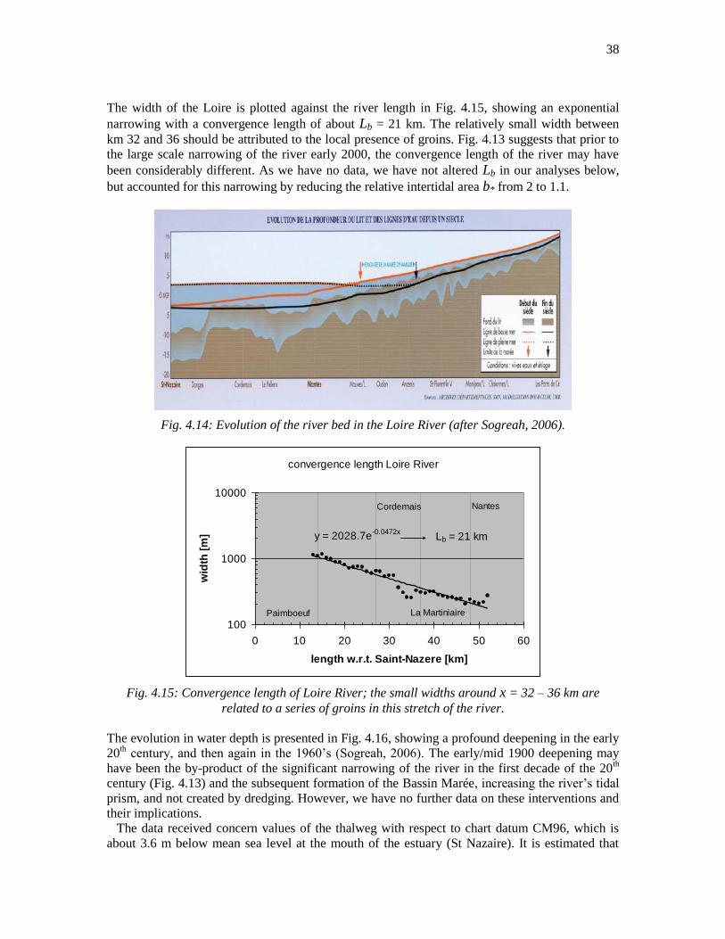
38

The width of the Loire is plotted against the river length in Fig. 4.15, showing an exponential

narrowing with a convergence length of about Lb = 21 km. The relatively small width between

km 32 and 36 should be attributed to the local presence of groins. Fig. 4.13 suggests that prior to

the large scale narrowing of the river early 2000, the convergence length of the river may have

been considerably different. As we have no data, we have not altered Lb in our analyses below,

but accounted for this narrowing by reducing the relative intertidal area b* from 2 to 1.1.

Fig. 4.14: Evolution of the river bed in the Loire River (after Sogreah, 2006).

convergence length Loire River

y = 2028.7e-0.0472x

100

1000

10000

0 10 20 30 40 50 60

length w.r.t. Saint-Nazere [km]

wid

th [

m] Lb = 21 km

Paimboeuf La Martiniaire

Cordemais Nantes

Fig. 4.15: Convergence length of Loire River; the small widths around x = 32 – 36 km are

related to a series of groins in this stretch of the river.

The evolution in water depth is presented in Fig. 4.16, showing a profound deepening in the early

20th century, and then again in the 1960’s (Sogreah, 2006). The early/mid 1900 deepening may

have been the by-product of the significant narrowing of the river in the first decade of the 20th

century (Fig. 4.13) and the subsequent formation of the Bassin Marée, increasing the river’s tidal

prism, and not created by dredging. However, we have no further data on these interventions and

their implications.

The data received concern values of the thalweg with respect to chart datum CM96, which is

about 3.6 m below mean sea level at the mouth of the estuary (St Nazaire). It is estimated that

39

MSL is about 0.3 m higher at Nantes, and the subsequent slope in MSL along the river has been

accounted for in Fig. 4.16. From an analysis of the data of the present bathymetry, it is estimated

that the thalweg lies about 1 – 2 m below the mean water depth (cross section divided by river

width), e.g. Deltares (2011). In the following we assume that the depth of Fig. 4.16 should be

raised by 1 m for the years 1900 – 1947, and with 2 m for the years thereafter – this has been

accounted for in the analyses below.

evolution water depths Loire River (thalweg)

2

4

6

8

10

1900 1920 1940 1960 1980 2000 2020

year

de

pth

w.r

.t. M

SL

[m

]

Paimboeuf - Cordemais

Cordemais - La Martiniere

La Martiniere - Nantes

Fig. 4.16: Evolution of water depth (thalweg) with respect to local mean water level (data

convergence: chart datum CM96 is 3.6 m below MSL at St Nazaire)..

evolution tidal amplitude Loire River

0

0.5

1

1.5

2

2.5

3

1900 1920 1940 1960 1980 2000 2020

year

am

pli

tud

e [

m]

km 0: St Nazeire

km 14: Paimboeuf

km 27: Cordemais

km 37: La Martiniere

km 48: Nantes

Fig. 4.17: Evolution of the tidal amplitude along the Loire River; the black box represents the

period of river narrowing (e.g. Fig. 4.13).

Note that the data of Fig. 4.17 are not very accurate, nor complete, so the analysis in this section

is not so accurate, in particular the developments later in the 20th century – more detailed data

have been requested.

The measured evolution in tidal amplitude is presented in Fig. 4.17, showing huge amplifications

of the tide in the first half of the 20th century. Though at a smaller rate, the tidal amplitude

continues to increase after the 1950s; at Nantes for instance by 0.7 m. In the following we focus

40

on the inner river (e.g. up-estuary of Paimboeuf) and subdivide the river further to the four tidal

stations along the river (Paimboeuf – Cordemais; Cordemais – La Martiniere; La Martiniere –

Nantes, e.g. stretches of 13, 10 and 11 km respectively).

From the data of Fig. 4.17 the evolution of the imaginary wave number can be established, the

results of which are shown in Fig. 4.18. Huge changes occurred in the early 20th century, no doubt

because of the canalization of the river in that period. From 1940 onwards, ki ≈ 0, i.e. the tide is

no longer damped in the Loire river. Note that signal is very strong and therefore consistent in the

early 20th century, but thereafter becomes a bit erratic. We believe that this is due to inaccuracies

of the data in general, and to ignoring the effects of the 18.6 year cycle (e.g. section 4.5).

evolution tidal amplification Loire River

-0.07

-0.05

-0.03

-0.01

0.01

1900 1920 1940 1960 1980 2000 2020

year

ki [

km

-1]

Paimboeuf - Cordemais

Cordemais - Martiniere

Martiniere - Nantes

Fig. 4.18: Evolution of the imaginary wave number, based on the tidal data of Fig. 4.17.

tidal evolution Loire

-3

-2

-1

0

1

0 1 2 3 4 5

estuarine convergence number e

rela

tiv

e d

am

pin

g

i

Paimboeuf - Cordemais

Cordemais - Martinaire

Martinaire - Nantesr* = 7.5

r* = 2.1

r* = 2.3

r* = 2.7r* = 3.2

r* = 3.8

Fig. 4.19a: Tidal amplification as function of convergence number

41

Next, the imaginary wave numbers of Fig. 4.18 have been made dimensionless with the

convergence length and plotted against the estuary convergence number e (equ. 8), the results of

which are shown in Fig. 4.19a. Time evolution is diagonally from the left lower corner to the

right upper corner of the figure. If we focus on the data beyond 1940 (omitting the three data

points with e > 2), we obtain Fig. 4.19b.

tidal evolution Loire

-0.5

-0.4

-0.3

-0.2

-0.1

0

0.1

0.2

0 0.2 0.4 0.6 0.8 1 1.2

estuarine convergence number e

rela

tive d

am

pin

g

i

Paimboeuf - Cordemais

Cordemais - Martinaire

Martinaire - Nantes

r* = 7.5

r* = 2.1

r* = 2.3

r* = 2.7

r* = 3.2

r* = 3.8

Fig. 4.19b: Tidal amplification as function of convergence number

evolution effective hydraulic drag Loire River

0

20

40

60

80

1900 1920 1940 1960 1980 2000 2020

year

Ch

ezy

[m

1/2

/s]

Paimboeuf - Cordemais

Cordemais - La Martiniere

La Martiniere - Nantes

Fig. 4.20: Evolution of effective hydraulic drag Loire estuary – note that because of low accuracy

of the tidal data, the error in this graph is relatively large.

42

Then, the linear model for an infinitely long tidal river (equ. 11) is fitted to the measured tidal

damping by tuning the effective dimensionless roughness coefficient r* to the data, e.g. Fig. 4.19a

and 4.19b.

From the fitted r*-values the effective Chézy coefficient can be obtained (equ. 8), using the

observed (corrected) water depths and estimated flow velocities – for the latter, we assume that U

= 1 m/s at the mouth of the river, and changes along the river in line with the imaginary wave

number).

Fig. 4.20 shows the variation in Chézy coefficient throughout the 20th century for the three river

stretches in the Loire. The Chézy coefficient in the first part of the estuary (Paimboeuf –

Cordemais) has basically remained constant over time at a value between 60 and 70 m1/2

/s.

However, in the upper two sections, the Chézy coefficient has increased from around 30 – 40

m1/2

/s till 60 – 70 m1/2

/s. The major changes took place in the period before 1940, when the

estuary was considerably narrowed. Note that the higher values are not very high, in particular

not for a very muddy system as the Loire – fluid mud is general observed between Cordemais and

Nantes (Sogreah, 2007). However, the historic data are too inaccurate to provide a better analysis

of the historic development of the Loire River.

Fig. 4.21: Computed (Sogreah, 2006) tidal amplitude(vertical axis) at Donges (upper panel, km

11) and Chantenay (lower panel, km 51) showing development of steepening of the rising tide.

Because of inaccuracies in the available tidal data it is not possible to obtain proper trends in the

-parameter with the analytical model. However, all information reveals that the tide in the Loire

43

has become highly asymmetrical. Whereas the tide in the mouth of the Loire River (observations

at Donge, e.g. Sogreah, 2006) is almost symmetrical, near Nantes rising tide takes place in about

4 hours, and falling tide is about 50% longer. These observations are corroborated by numerical

simulations by Sogreah (2006), results of which are presented in Fig. 4.21.

Note that the asymmetry in flow velocity is largely affected by the fresh water river flow, which

may be large. Hence, the effects of tidal asymmetry (both in peak velocity and internal mixing,

e.g. section 3.1) may be overruled by the effects of the river flow, inducing ebb dominance,

flushing mud from the system.

Sogreah, 2006) reports full flushing of the fluid mud from the river at prolonged (>12 days)

high river flows, e.g. around 2000 m3/s, conditions which may not occur each year.

44

4.3 The Elbe River

The Elbe River originates in the Karkonosze mountains of the Czech Republic and flows through

Germany over 630 km passing the city of Hamburg (largest German seaport) at about 110 km

from the mouth at Cuxhaven (North Sea). The mean annual fresh water discharge is about 700

m3/s with a variation range of 200 to 3600 m

3/s. The mouth of the estuary is characterized by a

narrow deep channel and a very wide tidal flood plain up to 2 m above LAT (Hakensand, Medem

sand, Norder Grunde), see also Admiralty Chart No. 3261. The total width of the mouth is about

15 km. The width of the deep channel is in the range of 1500 to 3000 m. The area below LAT of

the deep channel at the mouth is in the range of about 20000 to 40000 m2. Fig. 4.22 shows a plan

view of the river.

Fig. 4.23 presents the evolution of the tidal range along the Elbe River, as presented by Weilbeer

and Klöpper (2011), showing a considerable amplification of the tide upstream of kmr ~670/680

after the 1970’s. Initially, i.e. in the beginning of the century, the tide was damped over the entire

estuary.

Fig. 4.22: Plan view of lower Elbe river from Hamburg (kmr ~620) to Cuxhafen (kmr 724) and

kmr – co-ordinates along the river.

Fig. 4.23 suggests a discontinuity in tidal response around kmr 680. This is further substantiated

by the longitudinal variation in flow carrying cross section, presented in Fig. 4.24, showing a

substantial kink in this variation. In fact, the cross section in the outer part of the estuary is almost

constant, whereas the inner part follows a more exponential distribution. It is postulated that this

fairly uncommon distribution is the result of human interventions, in particular with respect to

embanking and reclamation.

45

tidal evolution Elbe River

100

200

300

400

580620660700740

kmr

tid

al ra

ng

e [

m]2001-2005

1991-1995

1981-1985

1971-1975

1961-1965

1951-1955

1911-1915

Fig. 4.23: Tidal amplification as function along Elbe River (after Weilbeer and Klöpper, 2011)

convergene of Elbe River

y = 0.005e0.0189x

100

1000

10000

600 625 650 675 700 725

distance [km]

wid

th [

m]

Lb = 53 km

Fig. 4.24: Longitudinal variation of flow-carrying cross section with discontinuity at kmr 670

(after Portal Tideelbe, 1999). The overall convergence length measures 53 km.

In the following, we distinguish between the inner and outer estuary, with their transition around

kmr 680. Because of a lack of sufficiently detailed data, we treat the outer and inner estuary as

two different, but homogeneous parts of the river. Then, based on the data of Fig. 4.23, the

variation in the imaginary wave number ki can be assessed for the two river parts, as shown in

Fig. 4.25. Fig. 4.25 also contains information on the design depth of the fairway in the Elbe

River, and the years in which the deepenings were realized. Note that we do not have data before

1940, though the Portal Tideelbe (chapter 3.3 Veränderungen am Flusz) states that in 1859 the

fairway was deepened to -5.9 m, whereas form 1910 a depth of 8 – 10 m have been maintained.

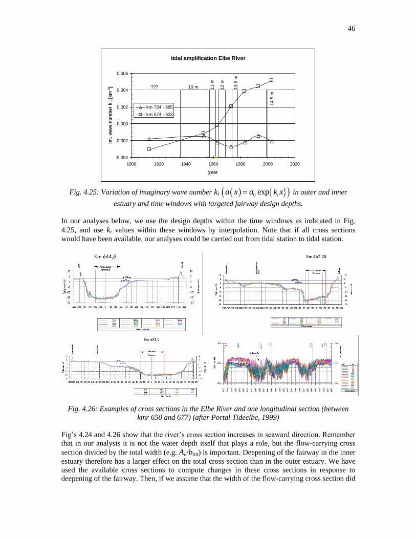
46

tidal amplification Elbe RIver

-0.004

-0.002

0.000

0.002

0.004

0.006

1900 1920 1940 1960 1980 2000 2020

year

im.

wave n

um

ber

ki [k

m-1

]km 724 - 685

km 674 - 623

10 m??? 11 m

14.5

m

13.5

m

12 m

Fig. 4.25: Variation of imaginary wave number ki 0 exp ia x a k x in outer and inner

estuary and time windows with targeted fairway design depths.

In our analyses below, we use the design depths within the time windows as indicated in Fig.

4.25, and use ki values within these windows by interpolation. Note that if all cross sections

would have been available, our analyses could be carried out from tidal station to tidal station.

Fig. 4.26: Examples of cross sections in the Elbe River and one longitudinal section (between

kmr 650 and 677) (after Portal Tideelbe, 1999)

Fig’s 4.24 and 4.26 show that the river’s cross section increases in seaward direction. Remember

that in our analysis it is not the water depth itself that plays a role, but the flow-carrying cross

section divided by the total width (e.g. Ac/btot) is important. Deepening of the fairway in the inner

estuary therefore has a larger effect on the total cross section than in the outer estuary. We have

used the available cross sections to compute changes in these cross sections in response to

deepening of the fairway. Then, if we assume that the width of the flow-carrying cross section did

47

not change over time, we can construct the evolution in mean depth for the outer and inner

estuary, e.g. Fig. 4.27.

Fig. 4.27 also depicts the development of the depth of the fairway showing a profound step in

depth near around Hamburg, in particular in later years (e.g. Kappenberg and Fanger, 2007).

evolution mean water depth Elbe River

10

11

12

13

1920 1940 1960 1980 2000 2020

kmr

me

an

de

pth

[m

] entire river

inner estuary

outer estuary

Fig. 4.27: Evolution of mean water depth along Elbe River. Fairway (upper panel) and mean

depth in outer and inner estuary.

Fig. 4.28 shows the longitudinal variation in width of the flow-carrying cross section along the

Elbe River, based on data provided by BAW (2012). The mean convergence length amounts to

about 53 km (Fig. 4.24), though the data show large scatter. However, as suggested by Fig. 4.24,

and the data of Fig. 4.28, the convergence length in the outer estuary is much larger than in the

inner estuary – in the following we will use two different lengths, i.e. 93 and 30 km in the outer

and inner estuary, respectively. In the inner estuary, the intertidal area seems to amount to about

20% and in the outer estuary about 60% of the width of the flow-carrying cross section (e.g. b* =

1.2 and 1.6, respectively). Note that from an inspection of Google Earth images, these numbers

are likely to be on the high side. A detailed analysis of the river’s hypsometry is required to

obtain more accurate data. Moreover, we have no information on how the intertidal area changed

over time.

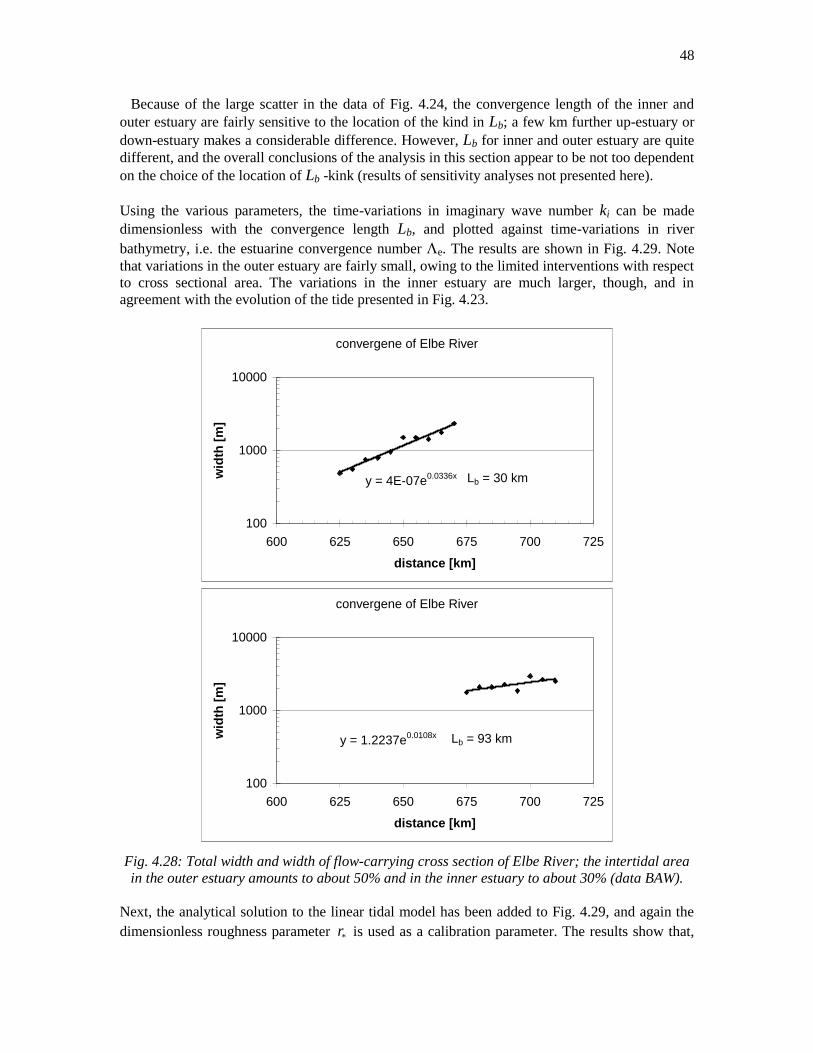
48

Because of the large scatter in the data of Fig. 4.24, the convergence length of the inner and

outer estuary are fairly sensitive to the location of the kind in Lb; a few km further up-estuary or

down-estuary makes a considerable difference. However, Lb for inner and outer estuary are quite

different, and the overall conclusions of the analysis in this section appear to be not too dependent

on the choice of the location of Lb -kink (results of sensitivity analyses not presented here).

Using the various parameters, the time-variations in imaginary wave number ki can be made

dimensionless with the convergence length Lb, and plotted against time-variations in river

bathymetry, i.e. the estuarine convergence number e. The results are shown in Fig. 4.29. Note

that variations in the outer estuary are fairly small, owing to the limited interventions with respect

to cross sectional area. The variations in the inner estuary are much larger, though, and in

agreement with the evolution of the tide presented in Fig. 4.23.

convergene of Elbe River

y = 4E-07e0.0336x

100

1000

10000

600 625 650 675 700 725

distance [km]

wid

th [

m]

Lb = 30 km

convergene of Elbe River

y = 1.2237e0.0108x

100

1000

10000

600 625 650 675 700 725

distance [km]

wid

th [

m]

Lb = 93 km

Fig. 4.28: Total width and width of flow-carrying cross section of Elbe River; the intertidal area

in the outer estuary amounts to about 50% and in the inner estuary to about 30% (data BAW).

Next, the analytical solution to the linear tidal model has been added to Fig. 4.29, and again the

dimensionless roughness parameter *r is used as a calibration parameter. The results show that,

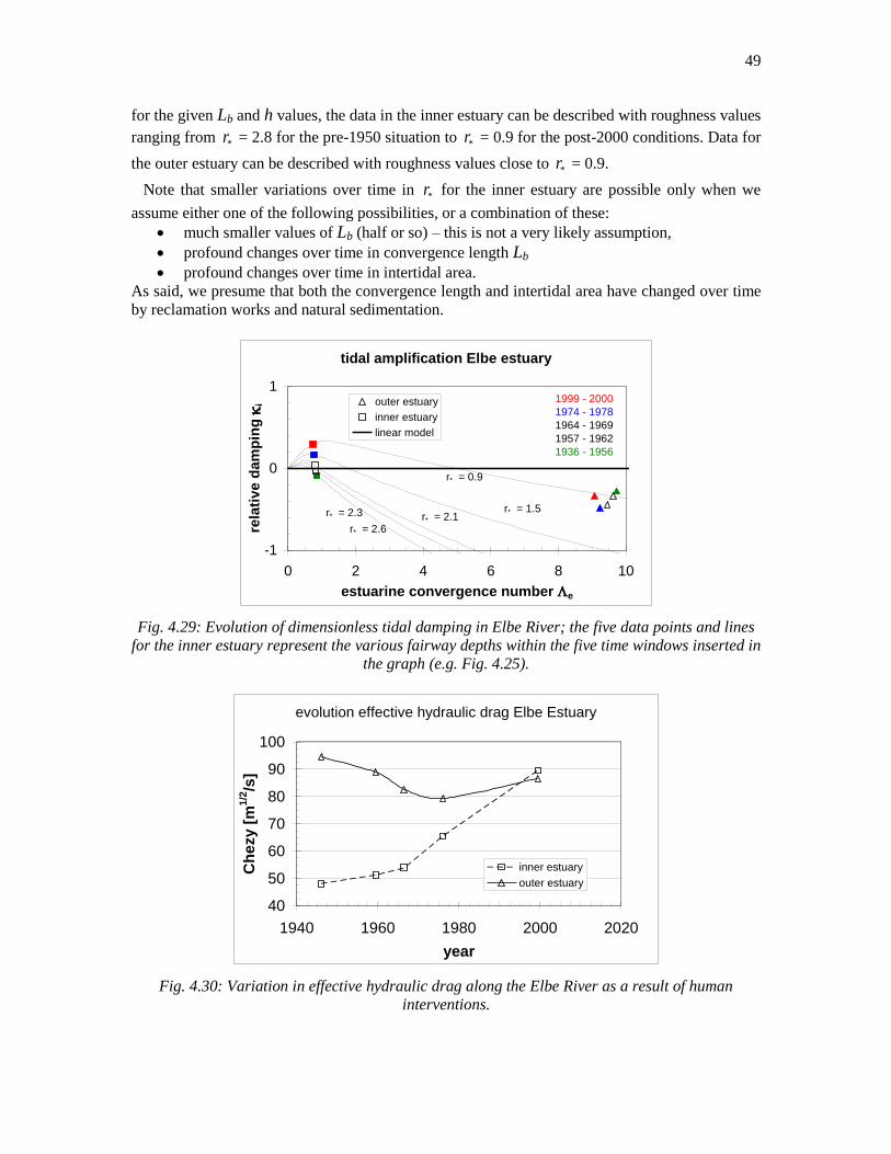
49

for the given Lb and h values, the data in the inner estuary can be described with roughness values

ranging from *r = 2.8 for the pre-1950 situation to *r = 0.9 for the post-2000 conditions. Data for

the outer estuary can be described with roughness values close to *r = 0.9.

Note that smaller variations over time in *r for the inner estuary are possible only when we

assume either one of the following possibilities, or a combination of these:

much smaller values of Lb (half or so) – this is not a very likely assumption,

profound changes over time in convergence length Lb

profound changes over time in intertidal area.

As said, we presume that both the convergence length and intertidal area have changed over time

by reclamation works and natural sedimentation.

tidal amplification Elbe estuary

-1

0

1

0 2 4 6 8 10

estuarine convergence number e

rela

tive d

am

pin

g

i outer estuary

inner estuary

linear model

1999 - 2000

1974 - 1978

1964 - 1969

1957 - 1962

1936 - 1956

r* = 2.6

r* = 2.3 r* = 2.1r* = 1.5

r* = 0.9

Fig. 4.29: Evolution of dimensionless tidal damping in Elbe River; the five data points and lines

for the inner estuary represent the various fairway depths within the five time windows inserted in

the graph (e.g. Fig. 4.25).

evolution effective hydraulic drag Elbe Estuary

40

50

60

70

80

90

100

1940 1960 1980 2000 2020

year

Ch

ezy

[m

1/2

/s]

inner estuary

outer estuary

Fig. 4.30: Variation in effective hydraulic drag along the Elbe River as a result of human

interventions.

50

From the dimensionless roughness parameter *r , a Chézy coefficient C can be established,

assuming that the damping in flow velocity is identical to the damping in tidal amplitude (as is

assumed in our linear model). Fig. 4.30 shows that in the outer estuary C remains around 80

m1/2

/s over time. However, in the inner estuary the results suggest that over time, the river

becomes very smooth, up to C ≈ 90 m1/2

/s in the 2000s.

The high Chézy-values in the outer estuary are in agreement with the high SPM-values in this

part of the river, and the very muddy intertidal areas (e.g. Fig. 4.31).

Another effect which may have reduced the effective hydraulic drag is the continuous off-

topping of the bed forms in the Elbe River by maintenance dredging. The longitudinal profile of

the river in the lower right panel of Fig. 4.26 reveals considerable bed forms of a few meter

height. Such bed forms were already described by Nasner (1974), reporting dune heights of 1 – 3

m, at lengths of 50 – 100 m, hence fairly steep. Such steep bed forms induce large effective

hydraulic drag (e.g. Van Rijn, 1990). These bed forms have decreased by about 1 dm or so, and

the reduction in effective hydraulic drag should therefore have been fairly limited.

Fig. 4.31: Variation in SPM-concentrations and salinity intrusion as a function of river flow

(after Kappenberg and Fanger, 2007). Down-estuary of kmr 670/680, SPM values are high, in

agreement with high Chézy-values; up-estuary, SPM-values are low.

51

Finally, it has to be noted that in our analytical, linear model, the effect of reflections of the tidal

wave have not been included. End of the 1950’s, the Geesthacht weir was erected, hence arresting

the tidal limit at about kmr 585. Furthermore, a distinct step in bed level around the port of

Hamburg developed over time, as hardly any deepening took place up-estuary of Hamburg

(Boelich and Strotmann, 2008). This is depicted in Fig. 4.27. A zero-order assessment of this step

in bed level was made by assuming full reflection at kmr 619 (Hamburg). Furthermore, the

analysis of the data suggest that in the course of the 1970s, the convergence of the inner estuary

has been decreased by river works. Therefore, we present results for Lb = 30 km and 40 km, e.g.

Fig. 4.32. All simulations have been carried out with r = 0.003 m/s (sandy riverbed).

tidal amplification with and without reflection at Hamburg

0.5

1.0

1.5

2.0

0 10 20 30 40 50

distance from kmr 670 [km]

tid

al a

mp

litu

de

[m

]

no relfection, h = 10 m, Lb = 30 km

no reflection, h = 10 m, Lb = 40 km

no reflection, h = 12 m, Lb = 30 km

with reflection, h = 10 m, Lb = 40 km

with reflection, h = 12 m, Lb = 30 km

Fig. 4.32: Computation of tidal amplitude for pre-1970 conditions (Lb = 40 km, broken line) and

post-1970 conditions (Lb = 30 km, full line).

From Fig. 4.32, the following conclusions can be drawn:

The amplification in the upper Elbe estuary is very sensitive to the convergence length Lb

– for Lb = 30 km, the linear model (only incoming wave) predicts amplification, whereas

for Lb = 40 km, damping is predicted.

For full reflection at kmr 619, the tide always amplifies – increasing the convergence

length does not have too much influence (results not shown). Only a large increase in

roughness (the r-parameter) reduces the amplification considerably.

The effect of amplification increases by a few dm’s upon deepening of the Elbe.

From these observations we may conclude that the increase in effective bed roughness in the

upper estuary (Fig. 4.30) is probably overestimated, as part of the amplification should be

attributed to reflections. However, it is not likely that full reflection takes place at Hamburg.

Moreover, these results suggest that the amplification of the tide in the (upper-)Elbe is quite

sensitive to the bathymetry and geometry of the river.

Next, the travel time of high water between Cuxhafen and Hetlingen (kmr 647, e.g. Fig. 4.33

upper panel) is computed using equ. (17). Computed and measured travel time are compared in

Fig. 4.33, showing that the linear model underpredicts the observed travel time by about 10%.

Analysis of the sensitivity of the travel time to model parameters showed that the travel time is

sensitive in particular to the convergence length, more than to the effective roughness. Hence, this

is another indication that the geometrical features of the Elbe are not known sufficiently well.

52

travel time Cuxhafen - Hetlingen (77 km)

0

1

2

3

0 1 2 3

measured [hrs]

co

mp

ute

d [

hrs

]

travel time

Fig. 4.33: Travel time high water in Elbe River; upper panel: observations in 1988; lower panel:

prediction by linear model

evolution tidal asymmetry

0.8

1

1.2

1.4

1940 1950 1960 1970 1980 1990 2000 2010

year

ga

mm

a

inner estuary

outer estuary

Fig. 4.34: Temporal variations in tidal asymmetry parameter in inner and outer estuary.

Finally, variations in tidal asymmetry have been assessed from variations in the -parameter, i.e.

the ratio of the wave celerity at high and at low water, in which the actually measured variations

53

in tidal amplitude have been used, in conjunction with the values for river depth h, convergence

length Lb, roughness r* and intertidal area b*, established and used above. Fig. 4.34 suggests that

the outer estuary remained ebb-dominant over time, whereas the inner estuary remained flood

dominant over time. These conclusions are more or less sustained with measurements of the

current velocity in Fig. 4.35, showing that in the outer estuary, the flow is slightly flood

dominant, but in the inner estuary flood-dominance is more pronounced. Note that the

underestimation of flood dominance (in the outer estuary) is likely the result of erroneous values

(too large) for the intertidal area b* - see also Boelich and Strotmann (2008).

Fig. 4.35: Measured tidal asymmetry along Elbe River; upper panel: near Brunsbuttel; lower

panel: near Schulau (after BAW, 2011)

It is to be noted that the flood dominance in the inner estuary follows a subtle interplay from a

decrease in by increased river depths, and an increase by tidal amplification. This would imply

that if the river were sub-divided into more sub-sections, we would expect a larger increase in

flood-dominance further upstream, near the port of Hamburg. As the riverine turbidity maximum

(RTM) is governed by tidal asymmetry and river-induced flushing, this would imply that:

the ETM moves upstream with decreasing river flow – indeed it has been observed that

dredging needs in the Port of Hamburg increase in years with low river flows (Haar,

1994).

over time, the ETM would have moved in upstream direction – unfortunately, we have no

information to confirm.

Our analysis of the data on the Elbe River suggest that:

1. The tide in the lower estuary (kmr 720 – 670) is largely influenced by a large intertidal

area, large convergence length and small effective hydraulic drag. Tidal amplification

over time remained relatively small.

2. The analysis with the linear model (infinitely long river) suggests a sharp increase in

Chézy coefficient in the inner estuary after 1970, suggesting a sharp increase in SPM in

54

the river. This is, however, not in agreement with the SPM data, which show relatively

low SPM-concentrations in this part of the river.

3. The Elbe river depicts a large step in water depth around Hamburg, which becomes more

pronounced over time (with deepening of the river). This step should induce reflections

of the tidal wave. Our model simulations, however, suggest that this can be only a partial

reflection.

4. We have no data on the convergence of the river prior to 1970. However, the analysis

with the linear model suggests that the river’s convergence has increased (Lb decreased).

5. The analyses indicate that the tidal propagation in the upper estuary is very sensitive to

the geometry and bathymetry of the river. This was confirmed by Weilbeer (2013). This

sensitivity itself suggest an important effect of reflections of the tidal wave, either at the

step in bed level around Hamburg, or otherwise.

However, these conclusions are based on a limited series of data, and further substantiation is

possible only upon further analysis. We recommend the following:

Make harmonic analyses of the historical tidal data at the various tidal stations along the

river (analysis should be done on M2 and M4 tidal component).

Make a proper analysis of the historic development of the river’s cross sections,

preferably in the form of hypsometric curves.

Make a detailed analysis of the development of convergence length and intertidal areas.

Analyze changes in bed forms, in particular variations in the steepness of dunes.

Analyze the changes in tidal amplitude in relation to geometrical changes along the river,

focusing on all sub-sections defined by the existing tidal stations.

Apply a (one-dimensional) numerical model to study the response of deepening,

reclamations, the step in bed level, Geesthacht weir and reduction in effective hydraulic

drag in a non-linear model, including possible reflections of the tidal wave.

55

4.4 The Weser estuary

Fig. 4.36: Overview of Weser estuary

We are in the process of acquiring data for the Weser River for an analysis similar to elsewhere in

this report. Hence, no results yet, though the enormous deepening of the river in the 20th century

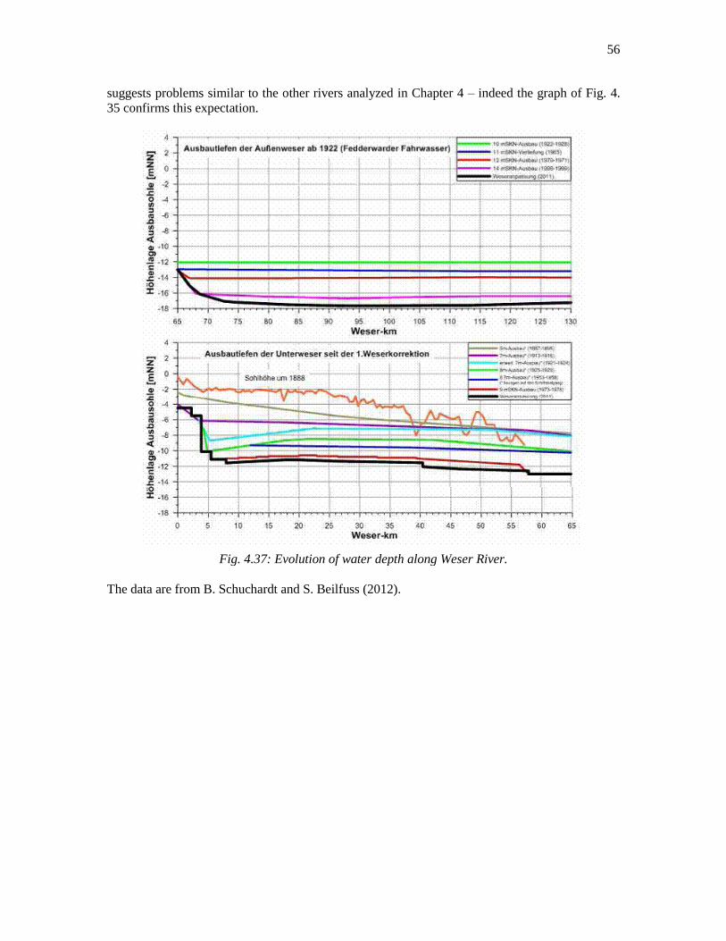
56

suggests problems similar to the other rivers analyzed in Chapter 4 – indeed the graph of Fig. 4.

35 confirms this expectation.

Fig. 4.37: Evolution of water depth along Weser River.

The data are from B. Schuchardt and S. Beilfuss (2012).

57

Fig. 4.38: Example of tidal amplification in Bremen over time

Currently, we have no further data available, and we cannot analyze the developments in the

Weser River. Yet, the amplifications are so large that we decided to include the results in this

report.

58

4.5 The Upper Sea Scheldt River (Boven Zeeschelde)

Fig. 4.39 shows an overview of the Scheldt estuary from its mouth near Flushing (Vlissingen) to

Ghent with indication of the various tidal stations treated in this report (see also Table 4.1, e.g.

IMDC, 2012). Further details, including the km-indications are given in Fig. 4.40.

Fig. 4.39: The Scheldt estuary from Flushing to Ghent with the various tidal stations.

Table 4.1: Summary of tidal stations along Sea Scheldt

Name km from Schelle km from Vlissingen

Schelle 0 91.2

Temse 7.5 98.7

Tielrode 11.9 103.1

Sint Amands 17.8 108.8

Dendermonde 30.6 121.8

Schoonaarde 41.7 132.6

Uitbergen 47.0 138.2

Wetteren 53.8 145.6

Melle 60.0 150.8

59

Fig. 4.40: Overview of Upper Sea Scheldt (Boven Zeeschelde) from Schelle (upper right corner)

to Melle (lower left corner).

Tidal data for the entire Scheldt estuary are available from before 1900. Kuijper (2012) corrected

these data for the 18.6 year cycle, the results of which are shown in Fig. 4.41a. In the following,

we focus on the Upper Sea Scheldt, i.e. up-estuary from Schelle. For an analysis of the time

evolution of the entire estuary, the reader is referred to Kuijper (2012, Western Scheldt) and

Plancke (2012, for Sea Scheldt). To allow further analysis, missing data points have been filled in

by interpolation from the available time and spatial series, e.g. Fig. 4.41b.3)

evolution tidal range along Scheldt estuary

Mell

e

Uit

berg

en

Sch

oo

naard

e

Den

derm

on

de

St

Am

an

ds

Tie

lro

de

Sch

ell

e

An

twerp

en

Lie

fken

sh

oek

Bath

Han

sw

eert

Tern

eu

zen

Vli

ssin

gen

Westk

ap

ell

e

1.50

2.00

2.50

3.00

3.50

4.00

4.50

5.00

5.50

-20 0 20 40 60 80 100 120 140 160

X [km]

tid

al

ran

ge [

m]

1901-1910

1911-1920

1921-1930

1931-1940

1941-1950

1951-1960

1961-1970

1971-1980

1981-1990

1991-2000

2001-2010

Fig. 4.41a: Evolution of tidal range along Scheldt estuary corrected for 18.6 year cycle.

3)

Note that no consistent analyses could be made using the original data, obtained by averaging and

grouping over decades – clear trends in tidal amplification and reflection could not be obtained.

60

evolution tidal range along Scheldt estuary

Mell

e

Uit

berg

en

Sch

oo

naard

e

Den

derm

on

de

St

Am

an

ds

Tie

lro

de

Sch

ell

e

An

twerp

en

Lie

fken

sh

oek

Bath

Han

sw

eert

Tern

eu

zen

Vli

ssin

gen

Westk

ap

ell

e

1.50

2.00

2.50

3.00

3.50

4.00

4.50

5.00

5.50

-20 0 20 40 60 80 100 120 140 160

X [km]

tid

al

ran

ge [

m]

1901-1910

1911-1920

1921-1930

1931-1940

1941-1950

1951-1960

1961-1970

1971-1980

1981-1990

1991-2000

2001-2010

Fig. 4.41b: Same as Fig. 4.41a, but missing data added by interpolation..

evolution of water depth Lower Sea Scheldt

-10.00

-8.00

-6.00

-4.00

-2.00

0.00

2.00

0 10000 20000 30000 40000 50000 60000

distance from Melle [m]

de

pth

[m

-TA

W]

y1930

y1960

y2001

y2009

100 per. Mov. Avg. (y1930)

100 per. Mov. Avg. (y1960)

100 per. Mov. Avg. (y2001)

100 per. Mov. Avg. (y2009)

Fig. 4.42: Evolution of water depth Upper Sea Scheldt w.r.t. TAW chart datum .

Van Braeckel et al. (2006) summarize modifications in the Scheldt estuary. The majority of the

engineering works in the Upper Sea Scheldt took place before 1900, e.g. rectifications of the river

and embanking intertidal areas. In the early 1900s (1900 – 1930) parts of the river were

normalized, and later rectifications took place in the Durme. In the 1970s, the river deepened by

1.5 – 2 m, e.g. Fig. 4.42, though no engineering works are reported. Possibly, this deepening was

the morphodynamic response to engineering works further down-estuary, such as sand-mining

and deepening and widening of Western-Scheldt and/or Lower Sea Scheldt. Also deepening and

61

widening of the Scheldt estuary down-estuary of Antwerp in the second half of the 20th century,

and early 21th century had an effect on the tidal evolution, as discussed below (see also Kuijper,

2012).

The evolution of the water depth in the Upper Sea Scheldt is further elaborated in Fig. 4.43

showing the water depth with respect to local mean water level, based on data from IMDC

(2012). The water depth in Fig. 4.43 is obtained from dividing the flow-carrying cross section by

the width of the river, and then averaging over the river sections in between the tidal stations.

evolution of mean water depth Upper Sea Scheldt

0

2

4

6

8

10

1920 1940 1960 1980 2000 2020 2040 2060 2080

year

de

pth

wrt

lo

ca

l M

SL

[m

] Schelle - Temse

Temse - St-Amands

St-Amands - Denderm.

Denderm - Schoonaarde

Schoonaarde - Wetteren

Wetteren - Melle

evolution of water depth Upper Sea Scheldt

0

2

4

6

8

10

80 100 120 140 160

distance from Flushing [km]

de

pth

wrt

lo

ca

l M

SL

[m

]

1930

1960

2001

2009

Fig. 4.43: Evolution of mean water depth between the various tidal stations along the Upper Sea

Scheldt.

At the head of the estuary, around Ghent, a number of engineering works were carried out

between 1950 and 1970. These works consisted of the creation of a new channel of about 4 km

length with a shipping lock for access to Ghent. Between around 1960 – 1970 the Upper Sea

Scheldt became deeper, and the old northern arm of the Upper Sea Scheldt has silted up largely.

The old Scheldt branch measured about 8.4 km from Melle tidal station to the weir in Ghent,

whereas the new branch measures about 7.2 km.

Fig. 4.44: Overview engineering works at head of Upper Sea Scheldt (Meersschaut, pers. com).

62

The convergence length of the Upper Sea Scheldt is plotted in Fig. 4.45, showing an exponential

behavior with a mean value of about 31 km, and little variation since 1930. Note that the river

rectifications in the late 19th century must have reduced this convergence length by about 5 km.

Fig. 4.45 suggests a kink in the river’s convergence between Dendermonde and Schoonaarde,

and the data have therefore been replotted in Fig. 4.46 showing a significant discontinuity in Lb.

However, no clear time signal can be identified.

convergence Upper Sea Scheldt

10

100

1000

0 10 20 30 40 50 60 70

distance from Schelle (= km 2) [km]

flo

w c

arr

yin

g w

idth

[m

] 1930

1960

2001

2009

Lb = 30 - 32 km

Fig. 4.45: Convergence length of Upper Sea Scheldt shows little variation since 1930.

convergence length Upper Sea Scheldt

10

100

1000

0 10 20 30 40 50 60 70

distance from Schelle [km]

flo

w c

arr

yin

g w

idth

[m

] 1930

1960

2001

2009

Lb = 22 - 26 km

convergence length Upper Sea Scheldt

10

100

1000

0 10 20 30 40 50 60 70

distance from Schelle [km]

flo

w c

arr

yin

g w

idth

[m

] 1930

1960

2001

2009

Lb = 32 - 40 km

Fig. 4.46: Convergence length of Upper Sea Scheldt for lower part (up to km 34) and upper part

(from km 34); km 34 is halfway Dendermonde and Schoonaarde.

Fig. 4.47 presents the total width of the Sea Scheldt River and its flow carrying width, again for

the lower and upper reaches. The total width is defined as the width of the river at the edges of its

salt marshes. Hence, this total width is expected to be a bit too large, as in our tidal analysis, the

mean high water level is relevant (see comment below). From a linear fit, we define a mean value

for b* for the upper and lower reaches.

Fig. 4.47 shows a continuous decrease in b* since 1850, in particular between 1850 and 1930 in

the upper reaches of the river. Note also that in the lower reaches, b* increases in upstream

direction, whereas in the upper reaches b* decreases in upstream direction (apart from the 1850-

data). This difference in trend may have a similar cause as discontinuity in convergence length,

discussed above.

63

It should be noted that, because of its definition with respect to the edges of the salt marshes, the

values in b* in Fig. 4.47 are likely to be an over-estimation of the actual values, which should be

related to the river’s width at mean high water. Moreover, it is likely that this over-estimation is

larger in recent years, because of siltation on intertidal mud flats and subsequent development of

vegetation owing to the high suspended sediment concentrations in the river. Visual inspection by

the author of this report suggests that in 2012 a large part of intertidal area has been lost in favor

of salt marshes.

convergence Sea Scheldt River;

Schelle - Dendermonde

10

100

1000

80 90 100 110 120 130 140

distance from mouth [km]

flo

w-c

arr

yin

g w

idth

[m

]

1850; Lb = 20 km

1930; Lb = 22 km

1960; Lb = 23 km

2001; Lb = 23 km

Dendermonde Schoonaarde

convergence Sea Scheldt River;

Dendermonde - Melle

10

100

1000

80 100 120 140 160

distance from mouth [km]flow

-carr

yin

g w

idth

[m

]

1850; Lb = 38 km

1930; Lb = 38 km

1960; Lb = 38 km

2001; Lb = 38 km

DendermondeSchoonaarde

0

2

4

6

8

10

80 90 100 110 120 130 140

tota

l w

idth

/ flo

w w

idth

distance from mouth [km]

convergence Sea Scheldt River; Schelle - Dendermonde

1850; mean b* = 2.3

1930; mean b* = 2.3

1960; mean b* = 2.1

2001; mean b* = 1.8

0

2

4

6

8

10

80 100 120 140 160

tota

l w

idth

/ f

low

wid

th

distance from mouth [km]

convergence Sea Scheldt River; Dendermonde - Melle

1850; mean b* = 4.6

1930; mean b* = 1.7

1960; mean b* = 1.6

2001; mean b* = 1.4

Fig. 4.47: Convergence length of flow carrying width (upper panel) and ratio total width over

flow-carrying width (lower panel) of lower reach of Sea Scheldt (Schelle – Dendermonde) and

upper reach (Dendermonde – Melle) since 1850.

Fig. 4.48 presents the imaginary wave number as derived from the measured tidal data of Fig.

4.41b, in which missing data points in the original data (e.g. Fig. 4.41a) have been added upon

interpolation. Fig. 4.48 shows a number of important trends:

From Schelle to halfway Dendermonde-Schoonaarde, the damping of the tidal wave

increases (ki more negative), and beyond ~km 125, the damping decreases again.

In general, the damping along most part of the river has decreased over time.

Close to Schelle, the tidal wave is no longer damped in the early 21th century.

64

evolution tidal damping Upper Sea Scheldt

-0.03

-0.02

-0.01

0

0.01

50 75 100 125 150

distance from Flushing km]

im. w

av

e n

um

be

r k

i [l

m-1

] 1901-1910

1911-1920

1921-1930

1931-1940

1941-1950

1951-1960

1961-1970

1971-1980

1981-1990

1991-2000

2001-2010

Dendermonde

Schoonaarde

Fig. 4.48: Evolution of imaginary wave number along Upper Sea Scheldt, based on the data of

Fig. 4.41b.

evolution tidal damping Upper Sea Scheldt

-0.03

-0.02

-0.01

0

0.01

50 75 100 125 150

distance from Flushing km]

im. w

av

e n

um

be

r k

i [l

m-1

]

1901-1910

1911-1920

1921-1930

1931-1940

1941-1950

1951-1960

1961-1970

1971-1980

1981-1990

1991-2000

2001-2010

Dendermonde

Schoonaarde

Fig. 4.49: Evolution of the imaginary wave number with time, and grouped for data from before

1960, after 2000, and in between. Time-mean values of data <1960 (black lines) yield ki,old.

Fig. 4.43 shows a profound deepening of the Upper Sea Scheldt between 1960 and 2001 (other

information suggests that this happened between 1960 and 1970). Therefore, the evolution of the

imaginary wave number ki has been replotted in Fig. 4.49, where the data have been grouped in

series before 1960 (black lines), after 2000 (red lines, and in between. Up to

65

Dendermonde/Schoonaarde, ki has increased with ~0.005 km-1

, further up-estuary, the trends are

less obvious.

Next, the imaginary wave number before 1960 has been averaged over time, yielding a time-

mean variation of ki with distance, referred to as ki,old. Let us next assume that the increase in

tidal amplitude at Antwerp is due only to deepening/widening of the Western Scheldt and the Sea

Scheldt in the vicinity of Antwerp, i.e. all river stretches down-estuary of Schelle. Then we can

“predict” the tidal evolution up-estuary of Antwerp, using the measured evolution of the tidal

range at Antwerp, and using ki,old. This prognostic tidal evolution is presented in Fig. 4.50, in

conjunction with the actual measured evolution, suggesting that the measured amplification from

Schelle till Dendermonde/Schoonaarde should be ascribed for about 30% to down-estuary

modifications of the Scheldt estuary, and for about 70% to changes in local bathymetry as

discussed in Fig 4.43. The anomalous behavior up-estuary of Dendermonde/Schoonaarde is

discussed below.

The change in longitudinal trend of the imaginary wave number beyond

Dendermonde/Schoonaarde in Fig. 4.49 is remarkable. To explain this trend, we have computed

the tidal amplitude over the river beyond Sint Amands without a weir and with a weir 8 km up-

estuary of Melle. We have assumed a constant convergence length and a mean depth of 4.5 m.

The results are presented in Fig. 4.51 in the form of the difference in imaginary wave number ki

between the configuration with and without weir, reproducing the reverse in trend of Fig. 4.49,

and an increase by about 0.005 km-1

, which is about a factor two too small. Note that these results

are not sensitive to the convergence length Lb, but highly sensitive to the water depth – the latter

varies considerably over the last part of the river, whereas no information is available on the

sections up-estuary of Melle. The results of Fig. 4.51 are therefore only indicative of effect of

tidal reflections on the tidal evolution,

computed evolution of tidal range, asuming no deepening Sea Scheldt

Mell

e

Uit

berg

en

Sch

oo

naard

e

Den

derm

on

de

St

Am

an

ds

Tie

lro

de

Sch

ell

e

An

twerp

en

Lie

fken

sh

oek

Bath

Han

sw

eert

Tern

eu

zen

Vli

ssin

gen

Westk

ap

ell

e

1.50

2.00

2.50

3.00

3.50

4.00

4.50

5.00

5.50

-20 0 20 40 60 80 100 120 140 160

X [km]

Tid

al

ran

ge [

m]

1951-1960

1961-1970

1971-1980

1981-1990

1991-2000

2001-2010

pred 61-70

pred 71-80

pred 81-90

pred 91-00

pred 01-10

Fig. 4.50: Prognostic tidal evolution along the Upper Sea Scheldt, based on the lower values of

the imaginary wave number of Fig. 4.49 (e.g. ki,old).

66

effect weir on damping in Upper Sea Scheldt

-0.005

0

0.005

0.01

0 50 100 150

distance from Flushing [km]

diffe

ren

ce

im

. w

ave

nu

mb

er

k

i [km

-1]

Dendermonde

Schoonaarde

Fig. 4.51: Estimate of effect of weir on tidal damping in upper reaches of Upper Sea Scheldt.

Next, the imaginary wave numbers of Fig. 4.49 are made dimensionless with the convergence

length of the Upper Sea Scheldt (e.g. equ. 8), where data up-estuary of Schoonaarde are omitted,

as these are affected too much by tidal reflection. The dimensionless damping is plotted against

the estuarine convergence number e in Fig. 4.52, showing a not too systematic trend with time.

Data from before the large deepening in the Upper Sea Scheldt (<1960), data beyond 1990 and

data in between have been marked with different colors. In particular, the data for the trajectory

Dendermonde – Schoonaarde are a bit erratic (results not shown), most likely because of the

effects of tidal reflection, and therefore not further included in our analysis.

evolution dimensionless damping Upper Sea Scheldt

-1.75

-1.25

-0.75

-0.25

0.25

0.5 0.7 0.9

estuarine convergence number e [-]

da

mp

ing

i [

-]

Schelle - Temse

Temse - St Amands

St Amands - Dendermonde

> 1991

1961 - 1990

< 1960

Fig. 4.52: Evolution of dimensionless imaginary wave number i with variations in estuarine

convergence number e.

Next, the linear model for an infinitely long tidal river (equ. 11) is fitted through the data by

tuning the roughness parameter r*, the results of which are presented in Fig. 4.53, showing

variations in r* from 9 to about 3.

To compute the effective hydraulic drag from the fitted r*-values, we need to make an

assumption on the flow velocity in the Upper Sea Scheldt. For this, we have used computational

67

results from the Delft3D model of the Western Scheldt, which show that the velocity amplitudes

at Antwerp are about 10% larger than at Flushing, for the current bathymetry. We assume that the

tidal velocities at Flushing have not changed much throughout the 20th century, and we assume

further that the evolution of the tidal velocities along the Scheldt estuary over time follow the

measured variations in tidal range, i.e. can be assessed from the imaginary wave number of Fig.

4.49. Then, by tuning r* fitting equ. (11) through the dimensionless data, and using the estimated

flow velocity and measured water depth, the effective Chézy coefficient can be established. The

variation of C with time along the lower part of the Upper Sea Scheldt is presented in Fig. 4.54.

All Chézy values are a bit low, which may be attributed to the fact that in the linear model many

physical features in the river (bends, bed forms, bank irregularities, local variations in river

topography and bathymetry, etc.) are missing. Also, estimates of the flow velocity are rather

crude, though errors in this estimate occur only under the root of the solution to C (equ. 8).

evolution dimensionless damping Upper Sea Scheldt

-1.75

-1.25

-0.75

-0.25

0.25

0.5 0.6 0.7 0.8 0.9 1

estuarine convergence number e [-]

dam

pin

g

i [-]

Schelle - Temse

Temse - St Amands

St Amands - Dendermonde

r* = 9

r* = 2.9

r* = 3.8r* = 4.5

r* = 6r* = 8

> 1991

1961 - 1990

< 1960

Fig. 4.53: Fits of linear solution trough observations tuning the roughness parameter r* in the i

– e diagram.

evolution hydraulic drag Upper Sea Scheldt

0

20

40

60

80

1900 1920 1940 1960 1980 2000 2020

year

Ch

ezy

[m

1/2

/s]

Schelle - Temse

Temse - St Amands

St Amands - Dendermonde

Fig. 4.54: Evolution of effective hydraulic drag (Chézy coefficient) with time,

68

Yet Fig. 4.54 suggests that the Chézy coefficient, hence effective hydraulic drag, did not change

for the river stretch St Amands – Dendermonde, but increased considerably, in particular over the

first part Schelle – Temse. If this reduction in drag would have been caused by high suspended

sediment concentrations, this analysis suggests that values in SPM have been large for many

decades, which, in conjunction with further deepening (e.g. Fig. 3.3) may explain the increase in

C. The anomalous behavior between 1970 – 1990 is not understood, but may be misleading, as

topographic/bathymetric data over that period is missing, and had to be manufactured by

interpolation from other decades (see also bed level data of Fig. 4.43).

Fig. 4.55 presents measured data on tidal asymmetry, in the form of the ratio of the period of

rising tide and falling tide, showing flood dominance over the entire river, Plancke et al. (2012). It

is observed that flood dominance increases in upstream direction, as expected, as water depth

decreases in upstream direction. We note that the river fresh water flow is relatively small, hence

does only slightly affect the duration of flood and ebb period.

Ratio duration rising tide and falling tide - tidal asymmetry

0.0

0.2

0.4

0.6

0.8

1.0

1.2

1900 1920 1940 1960 1980 2000 2020

year

Ra

tio

Tri

sin

g/T

fall

ing [

-]

Bath

Liefkenshoek

Antwerpen

Schelle

Tielrode

St Amands

Dendermonde

Schoonaarde

Uitbergen

Melle

Fig. 4.55: Observed tidal asymmetry in Sea Scheldt.

However, it is remarkable that the asymmetry changes little over time, except may be for Schelle,

given the large increase in tidal amplitude. This discrepancy can be explained from two

developments:

1. In particular in the upper reaches, the water depth has increased largely in a relative

sense. Larger water depth would decrease tidal asymmetry, counteracting the effects of a

larger tidal range.

2. Probably more important is the development of tidal asymmetry in the Western Scheldt,

e.g. Fig. 4.55, which serves as “boundary conditions” for the Upper Sea Scheldt. Hence,

further to local generation of overtides in the Upper Sea Scheldt, tidal asymmetry is

“imported” from the down-estuary reaches of the estuary, i.e. the Western Scheldt.

It is beyond the present study to evaluate the evolution of tidal asymmetry in the Western Scheldt,

but the behavior of the asymmetry at Hansweert is remarkable, suggesting that its asymmetry

tends to re-establish the conditions at the beginning of the 20th century.

69

5. Summary and conclusions

This report describes an analysis of the historical development of the tide in a number of

European estuaries in relation to the human interventions (deepening, narrowing, rectifications,

….) carried out during the last century. The rationale behind this study is a fear that the Upper

Sea Scheldt (Belgium, river stretch between Schelle and Ghent) may develop into a hyper-turbid

system, such as the Ems and Loire rivers. This study is set up as follows:

1. Data of various tidal rivers have been collected. This was not always successful, and at

the moment this report was written, more or less reliable/accurate data are available from

the Ems, Elbe, Loire and Upper Sea Scheldt.

2. An analytical model has been derived, computing tidal propagation in estuaries.

3. This analytical model was then used to assess in a conceptual way the response of tidal

rivers to human interventions.

4. Finally, that model has been used to analyze the measured historical development of the

tide in the four rivers mentioned under 1.

This section summarizes the generic findings of this study, comparing the behavior of the various

rivers; the conclusions with special focus on the Upper Sea Scheldt (Boven Zeeschelde) are given

in the Dutch Samenvatting above.

In our analysis, two physical mechanisms are implicitly accounted for:

I. The effective hydraulic drag in a (tidal) river decreases and the friction length

increases when the water column becomes stratified. Such stratification occurs at

depth-averaged concentrations of fine suspended sediment of a few 100 mg/l.

Winterwerp et al. (2009) quantified this effect in a semi-analytical way. This work

suggests that the increase in Chézy coefficient, for the rivers treated in this report,

would amount to 15 – 30 m1/2

/s – this increase is linearly proportional with the

absolute water depth.

II. In an estuary, two turbidity maxima (ETM, estuarine turbidity maximum) may occur.

The first maximum, ETM1, the classic one referred to in all text books on estuaries,

is the result of a balance between river-induced flushing and up-estuary transport of

fine sediment by estuarine circulation (induced by the longitudinal salinity gradients),

and possibly some tidal asymmetry. This ETM1 is found in all “normal” estuaries

near the estuary’s mouth at the head of the salinity intrusion.

However, a second may be formed further up-estuary, which is governed by a

balance between river-induced flushing and up-estuary transport by tidal asymmetry

(both peak velocities and vertical mixing, i.e. internal asymmetry).

As a result of large changes in the river (deepening, human interventions), such a

second ETM2 can develop in a river previously characterized by an ETM1. Because

ETM1 and ETM2 are driven by different physical processes, and because both

ETM’s are fairly stable, we can refer to a regime shift when such a second ETM2

develops. These two regimes are sketched in Fig. 5.1.

The analytical model consists of the analytical solution of the one-dimensional shallow water

equations, i.e. continuity and momentum equations, describing the water movement in tidal

rivers. Note that the effects of river flow cannot be taken into account. These equations have been

linearized by omitting within the momentum equation the advection term, and by making the

friction term linear in the velocity. The solution to this set of equations is given in the form of a

wave number as a function of the estuarine convergence number, introduced in this report, and

the effective hydraulic drag. The wave number consists of a real part, reflecting the tidal wave

length, and an imaginary part, reflecting the damping or amplification of the tide in the estuary.

The plan form shape of the estuary (e.g. width, intertidal area), and its depth are given by the

70

estuarine convergence number. We assume that the width of the estuary converges in an

exponential way, an assumption almost always met in alluvial estuaries. The solution of the

analytical model is given in dimensionless numbers allowing mutual comparison of rivers of

rather different size. The analytical solution describes the behavior of an incoming tidal wave,

and its reflection, if relevant. In this study, the reflected wave is ignored in most cases, as the

underlying equations cannot be solved anymore analytically in case of non-constant depths along

the river. Note that an analytical solution is not possible either, when the water depth varies

arbitrarily along the river.

We also determined the celerity of the tidal wave through the estuary, and the phase difference

between water level and flow velocity, as well as a proxi for the tidal asymmetry from the

analytical model. In the major part of the work we assume an infinitely long river, unless stated

otherwise.

Fig. 5.1: Sketch of Estuarine Turbidity Maximum (ETM); ETM is characterized by a balance

between river-induced flushing and estuarine circulation (and some tidal asymmetry), and ETM2

by a balance between the effects of river-induced flushing and tidal asymmetry.

The analytical model is used in two ways:

I. Changes in tidal range (amplitude) and tidal asymmetry are computed as a function

of hypothetical changes in the surface of intertidal area, the convergence length of the

estuary, its depth, and the effective hydraulic drag. This provides a conceptual picture

on the river’s response to deepening and narrowing.

II. The measured historical evolution in tidal range is evaluated and linked to the

historical changes in the shape and bathymetry of the estuary:

For all time periods available, the damping/amplification of the tide along a

stretch of the river, bordered by two neighboring tidal stations, is computed in the

form of the (dimensionless) imaginary wave number.

The data on historical interventions in the rivers (deepening, narrowing, etc.) are

summarized in the estuarine convergence number – this number increases with

increasing water depth, increasing convergence of the river’s plan form and

decreasing intertidal area.

The historical development of the imaginary wave number is plotted against the

evolution of the estuarine convergence number. Each data point in that diagram

is obtained from actual observations, and represents one river stretch over a

specific period of time.

The analytical model is fitted through these data points by tuning the roughness

parameter of the model. Hence, the historical evolution in effective hydraulic

roughness is established.

Finally, the historical changes in tidal asymmetry are assessed on the basis of

actual observations or with the analytical model.

71

The response of a tidal river to deepening and narrowing, as computed with the analytical model,

is presented in Fig. 5.2 and 5.10. It is assumed that the estuary is infinitely long, than the initial

suspended sediment concentrations are low, and that the riverbed is sandy. Furthermore, it is

assumed that intertidal areas are present along the entire length of the river – the width of the

intertidal area equals the width of the flow-carrying section. The relative tidal amplitude at 60 km

from the mouth increases monotonously with depth, as shown by the black line in Fig. 5.2.

Without intertidal area, for instance upon embanking or reclamation, the increase in tidal

amplitude is somewhat larger, e.g. the blue line in Fig. 5.2.

tidal amplitude at 60 km relative to tidal amplitude at river mouth (= 1 m)

0.0

0.5

1.0

1.5

0 5 10 15 20

water depth [m]

tid

al a

mp

litu

de

at

60

km

[m

]

sand bed, with intertidal area

muddy bed, without intertidal area

sand bed, without intertidal area

Fig. 5.2: Response of tidal amplitude as function of the presence of an intertidal area and mud in

the water column, or on the River bed.

tidal asymmetry at x = 25 km from the mouth

0.0

0.5

1.0

1.5

2.0

0 5 10 15 20

water depth [m]

muddy bed, without intertidal area

sand bed, with intertidal area

sand bed, without intertidal area flo

od

do

min

an

teb

b d

om

inan

t

Fig. 5.3: Response of tidal asymmetry (-parameter) as function of the presence of an intertidal

area and mud in the water column, or on the River bed.

A more important response of the river, however, is presented in Fig. 5.3. With intertidal area, the

tide is always ebb-dominant, i.e. time-averaged transports of fine sediment are directed down-

estuary (black line Fig. 5.3). Note that we do not address the role of a possibly externally

generated tidal asymmetry. After loss of the intertidal area, the system becomes flood-dominant.

This implies that mud is pumped into the estuary and/or that riverine mud accumulates within the

estuary. Upon deepening, also the flushing capacity of the river decreases. The conditions for an

72

ETM2 (Fig. 5.1) are being created. With increasing suspended sediment concentration the

effective hydraulic drag decreases (Chézy coefficient increases), in response of which the tide is

further amplified (red line in Fig. 5.2). This then results in an increase in flood-dominance of the

system (red line Fig. 5.3), enhancing suspended sediment concentrations and decreasing the

effective hydraulic drag further. This positive feed-back loop induces a snowball effect.

This snowball effect is sketched in Fig. 5.4. One could argue that the loss of intertidal area has

reduced the resilience of the river – with intertidal area, the tide will be amplified upon deepening

of the river, but the system remains ebb-dominant, and the dangerous decrease in hydraulic drag

is not initiated, and ETM2 conditions are not generated.

Fig. 5.4: The feed-back loop (snowball effect) for deepening of low-resilient estuaries.

summary tidal evolution

0

2

4

6

1875 1900 1925 1950 1975 2000 2025

year

tid

al ra

ng

e [

m]

Antwerp

Bremen

Hamburg

Nantes

Papenburg

Fig. 5.5: Summary of tidal amplification in the 19th century in a number of European ports.

Whether ETM2 conditions actually will occur, and the time span over which this would happen,

is dependent on the amount of fine sediment (mud) available. The time between the creation of

“favorable” conditions and the actual occurrence of an ETM2 (hyper-turbid conditions) can be

long, up to decades. The loss in intertidal area (loss of resilience) took place mainly in the late

19th and early 20

th century throughout Europe, whereas profound deepenings took place in the

second half of the 20th century. The loss of intertidal area affects the resilience of the river in two

ways:

1. Loss of intertidal area increases the tidal amplitude upon deepening and induces flood-

dominant conditions (the latter effect is the more important),

73

2. Loss of intertidal area causes a loss of accommodation space for the sedimentation of fine

sediment – fine sediments brought into the system owing to the river’s flood-dominance

can only remain within the water column, as a result of which the effective hydraulic

roughness decreases, and the snowball effect of Fig. 5.4 can be initiated.

In this report the tidal evolution of four rivers has been analyzed, as these are the rivers from

which sufficient (historic) data were available. This evolution can be summarized with the

evolution of the tidal range at the major ports within these rivers – the accessibility of these ports

has been the driving force behind the deepening. The results are presented in Fig. 5.5, showing

increases in tidal range varying from 1 to 4 m. Note that all rivers have evolved to tidal conditions

known as macro-tidal.

evolution tidal amplification with time

-3.0

-2.5

-2.0

-1.5

-1.0

-0.5

0.0

0.5

0.1 1 10

estuarine convergence number e [-]

rela

tiv

e d

am

pin

g

i [-

]

Ems outer estaury

Ems inner estuary

Elbe outer estuary

Elbe inner estuary

Loire C-P (outer)

Loire M-C (middle)

Loire N-M (upper)

Scheldt Schel-Tem

Scheldt Tem-StAm

Scheldt StAm-Dend

r* = 0.8

r* = 1.1

r* = 1.5

r* = 1.8

r* = 3.5

r* = 7

C = 40 - 90 m1/2

/stime

Fig. 5.6: Comparison of historic evolution of dimensionless damping coefficient and estuarine

convergence number for four European rivers. Both time and Chézy coefficient follow a diagonal

from the lower right to the upper left; i > 0 implies amplification of the tide.

Fig. 5.6 summarizes the calibration of the analytical model by fitting the roughness parameter r*

through the various data points, presented in the dimensionless forms of the relative damping i

and the estuarine convergence number e. All rivers show an increase in r* with time, i.e. when

the rivers are more and more deepened.

This decrease in effective hydraulic drag is further illustrated with the evolution of the computed

Chézy coefficient for the four rivers and the various reaches of the river which could be

identified. This evolution is presented in Fig. 5.7, showing that the majority of the river reaches

have experienced a considerable increase in Chézy coefficient, by about 15 – 30 m1/2

/s – it is

anticipated that the majority of this increase is due to increased levels of suspended sediment

concentration. The larger increase has been established for the upper part of the Elbe River. This

can be explained by the larger depth of that river, as predicted by the semi-analytical relation on

74

the dependency of the effective hydraulic drag on suspended fine sediment concentrations. The

large Chézy-values found for the inner Elbe estuary are not related to high SPM-concentrations –

these have not been measured in this part of the river. However, our analysis suggests that the

inner Elbe is close to resonance conditions, hence very sensitive to small changes in bathymetry.

This resonance cannot be accounted for by the analytical model. Hence the tidal amplification

induced by resonance is captured by a very low friction coefficient, which therefore is likely to be

erroneous.

It is noted that all rivers show profound flood-dominant conditions – this follows from both the

analytical model, as from observations on flow velocities and/or the duration of rising vs falling

tide.

The computed increase in Chézy coefficient has been summarized in Fig. 5.15, together with

some data made available by prof. Townend (Thames, Mersey and Severn) and data from the

Gironde (Villaret et al., 2011) and the Western Scheldt ((Kuijper and Lescinski, 2012). From the

red data points we know that the river experiences serious problems with high concentrations of

fine sediment, whereas no excess Chézy values have been established for the green points – here

the river still behaves “normal”. Fig. 5.15 suggests that a diagonal line can be drawn in that graph

representing the tipping point/zone for the establishment of hyper-turbid conditions. However,

unless this shift in behavior is further supported by additional data and/or research, the reddish

line in Fig. 5.15 remains fairly speculative. Prandle (2003) found a similar decrease in friction

factor for muddy systems, but he related the friction coefficient f to the mud content of the bed;

data in his paper are incomplete to add to the current analysis.

evolution effective hydraulic drag Elbe Estuary

40

50

60

70

80

90

100

1940 1960 1980 2000 2020

year

Ch

ezy

[m

1/2

/s]

inner estuary

outer estuary

evolution of effective hydraulic drag Ems River

0

20

40

60

80

100

1940 1960 1980 2000 2020

year

Ch

ezy [

m1

/2/s

]

Emden - Leeroort

Leeroort - Papenburg

evolution effective hydraulic drag Loire River

0

20

40

60

80

1900 1920 1940 1960 1980 2000 2020

year

Ch

ezy [

m1/2

/s]

Paimboeuf - Cordemais

Cordemais - La Martiniere

La Martiniere - Nantes

evolution hydraulic drag Upper Sea Scheldt

0

20

40

60

80

1900 1920 1940 1960 1980 2000 2020

year

Ch

ezy

[m

1/2

/s]

Schelle - Temse

Temse - St Amands

St Amands - Dendermonde

Fig. 5.7: Summary of evolution of computed Chézy coefficient with time for four European rivers.

We have not yet been able to quantify the tipping point for the response of the estuaries to human

interventions, e.g. narrowing and deepening. However, a change in effective hydraulic drag may

be a useful indicator. This drag can be obtained from an analysis of tidal data, as in this report, or

75

from the use of numerical hydraulic models, in which the (effective) roughness coefficient is

tuned in the calibration of the model.

Fig. 5.8 suggests that this is indeed a versatile way forward, but currently we have four data

point only, if we assume that the Ems, Loire and Elbe river have passed the tipping point, and the

Upper Sea Scheldt not.

effecitve hydraulic drag of various rivers

25

50

75

100

125

0 5 10 15 20

characteristic water depth [m]

Ch

ezy c

oeff

icie

nt

[m1

/2/s

]

C = 18log(12h/ks)

hyper-turbid

"normal"

1

2

14

10

9

8 65

137

124

3

1811

16

17

15

Fig. 5.8: Comparison of effective hydraulic drag in some rivers as a function of water depth. The C-h

relation is based on ks = 2 and 5 cm, arbitrary values. Red symbols depict hyper-turbid conditions, green

symbols “normal conditions, and blue symbols possibly transitional systems; open symbols reflect

historical data. 1: Elbe-outer; 2: Elbe-inner; 3: Ems/E-L; 4: Ems/L-P; 5: Loire/P-C; 6: Loire/C-laM;

7: Loire/LaM-N; 8: Scheldt/S-T;9: Scheldt/T-StA; 10: Scheldt/StA-D; 11: Thames; 12: Severn-inner;

13: Severn-outer; 14: Western Scheldt; 15: Gironde-outer; 16: Gironde-inner (Villaret et al., 2011);

17: Yangtze estuary; 18: Vilaine (Vested et al., 2013). Note that data on Elbe-inner may be spurious

because of tidal reflections, as discussed in Section 2. Furthermore it is presumed that the turbidity

maximum in the Loire River used to be located in the outer Loire (pt 5).

This argument is further sustained by Table 5.1 in which a series of natural macro-tidal estuaries

and heavily engineered systems are given. This table suggests that macro-tidal conditions and

abundant availability of fine sediments are necessary conditions for initiation of the regime shifts

described above. It seems therefore useful to gather data on the (effective) hydraulic drag of the

rivers in Table 5.1, and add these to Fig. 5.8.

A final observation relates to the effects of climate change. With increasing sea level, water

depths increase, which induce similar effects as a deepening of the river. However, the major

impact is most likely a further squeezing of the river, reducing intertidal areas further, thereby

reducing the resilience of the system.

76

Table 5.1: Comparison of natural, macro-tidal rivers with (very) high suspended sediment

concentrations and heavily engineered estuaries. This table suggests that by engineering

estuaries too much, their regime is shifted from the left column to the right column.

deepened and narrowed natural macro-tidal rivers

Ems (Germany) +++ Amazon mouth (Brazil) +++

Elbe (Germany) ++ Alligator River (Australia) ++

Garonne (France) ++ Bay of Fundy (Canada) +++

Loire (France) +++ Bay Saint Malo (France) +++

Ouse (UK) ++ Jiaojiang River (China) ++

Seine (France) +/++ Mersey (UK) +++

Trent (UK) ++ Severn River (UK) +++

Vileine (France) ++

Weser (Germany) +/++

Western Schelde +

Upper Sea Scheldt ++

+++ hyper-turbid conditions

+ “normal” estuarine conditions

77

6. Recommendations

The analysis of historical data of four rivers with a linear, analytical model has revealed a

profound positive feed-back between the tidal properties and suspended fine sediment. This

analysis also suggest the existence of a tipping point, beyond which a tidal river evolves more or

less autonomously to a hyper-turbid state – such a tipping point could be passed upon extensive

engineering works (deepening, narrowing, …) in a tidal river. However, this tipping point could

not be quantified, nor was it possible to define indicators identifying the passage of a tipping

point. Possibly this tipping point can be identified from a thorough stability analysis of the

governing equations. This, however, requires a major study, and for the time being we propose to

try and quantify the tipping point in a more empirical way. For that, the following activities are

required:

1. Collect historical tidal data from more rivers, preferably in a variety of states, i.e. from

hyper-turbid to “normal”. These data should be analyzed in a way similar to the method

followed in the current report. Moreover, the analysis of the Loire can be improved if

more accurate data become available.

2. The analysis in the current report should be confronted with (historical) data on

suspended sediment concentration and/or maintenance dredging volumes to substantiate

the conclusions on mud-induced decreases in effective hydraulic drag.

3. Collect data/numbers from numerical models calibrated to simulate the tidal propagation

in large tidal rivers properly. Unexpectedly low values for the effective hydraulic drag

may indicate large suspended sediment concentrations. The calibrated values of the

roughness values can be added to our diagram on excess Chézy values to substantiate that

diagram further.

4. The amplification in some of the rivers in general, and within the upper part of the Elbe

river (up to Hamburg) seem to be affected considerably by wave reflections and/or

resonance. Because of the large effect of tidal amplification on tidal asymmetry, hence on

the fine sediment dynamics, it is recommended to study the reflections of tidal waves in

these estuaries further.

5. Set up numerical hydrodynamic models of the various rivers – it is anticipated that one-

dimensional models (SOBEK) are sufficient for the analyses required:

The effects of longitudinal variations in bathymetry (depth, intertidal area) can be

studied in a more realistic way.

The effect of the construction of weirs cannot be studied properly with the analytical

model, but is easily addressed with a numerical model.

The effects of river flow cannot be studied with the analytical model, but is easily

addressed with a numerical model.

A numerical model will also provide more sound information on the tidal asymmetry,

whereas with the analytical model, only a proxi can be established.

The computational results from the one-dimensional model can be analyzed in the same

way as in the current report, tuning the effective roughness coefficient to calibrate the

model.

6. Both the analytical and numerical model can be used, assessing the efficiency of

mitigating measures, such as those suggested for the Scheldt River.

7. It is recommended to study the causes of the deepening of the Upper Sea Scheldt in the

1970’s – this should be done with a morphodynamic model, including Lower Sea

Scheldt, and possibly (part of ) the Western Scheldt.

78

Acknowledgements

This work was carried within the framework of the LTV-project, which is the acronym for Long-

Term Vision of Scheldt estuary with respect to Safety, Accessibility and Nature, in which the

following sub-projects are integrated: Maintaining fairways Scheldt estuary, Permits for disposal

of dredged sediments and the so-called KPP (knowledge of primary processes) program of

Rijkswaterstaat. The study was financed by the Flemish “Afdeling Maritieme Toegang” and the

Dutch Ministry of Infrastructure and Environment, Rijkswaterstaat, Waterdienst and Directorate

Zeeland.

The results in this report are based on a large number of data from a variety of sources. Some data

sets were available at Deltares in reports, or in digital form from studies carried out earlier. Other

data have been prepared and made available especially for this project. I would like to thank the

following people for their support and supply of data: Dr. Alexander van Braeckel (INBO,

Brussels), ir. Gijsbert van Holland (IMDC) and Frederik Roose (Flemish Government) for

Scheldt data, Dr Frank Kösters (BAW Hamburg) for data on the Ems, Elbe and Weser rivers, dr.

Luc Hamm (Sogreah) for data on the Loire, and dr. Harro Heijer, Dr. Frank Koesters and dr. Jens

Jürgens (BAW) for data on the Ems, Weser and Elbe river; and Prof. Ian Townend for data on the

Thames and Severn estuaries.

I would like to thank the reviewers dr. Henk Schuttelaars (Delft University of Technology) and

prof. dr. Tom de Mulder (University of Ghent, Belgium).

79

References

BAW, 2012. Data received from Dr. Frank Koesters and dr. Jens Jürgens on Ems and Elbe.

Boelich M.J. and T. Strotmann, 2008. The Elbe estuary. Source unknown.

Briere, C., J. Crebas, A. Becker and J.C. Winterwerp, 2012. Analyse de la morphologie du chenal

de Nantes et étude de sa restauration - Phase 3 : Etude de l'impact d'une intervention à

l'amont de Nantes sur les caractéristiques de la marée. Deltares report 1201695 (in French).

Bruens, A.W., J.C. Winterwerp, C. Kranenburg, 2012. “Physical and numerical modeling of the

entrainment by a high-concentrated mud suspension”, ASCE, Journal of Hydraulic

Engineering, in press, doi:10.1061/(ASCE)HY.1943-7900.0000545.

Chandramohan, P.V., 1989. Density currents and siltation – with particular reference to Cochin.

IHE, Master Thesis, Delft, The Netherlands.

Deltares, 2011. Analyse de la morphologie du chenal de Nantes et étude de sa restauration - Phase

1 : Evolutions passées et fonctionnement actuel. Report 1201695-001.

Dankers, P.J.T., J.C. Winterwerp, 2007.“Hindered settling of mud flocs: Theory and validation.

Continental Shelf Research, 27, 1893-1907.

Dronkers, J. (1986). Tide-induced residual transport of fine sediments. In Van de Kreeke, J.:

Physics of Shallow Estuaries and Bays, 228-244, Springer, Berlin.

Dronkers, J., 2005. Dynamics of coastal systems. Advanced Series on Ocean Engineering – Vol

25. World Scientific.

Dyer, K. R. 1997, Estuaries: a physical introduction. Chichester, England. John Wiley and Sons.

Friedrichs, C., 2010. Barotropic tides in channelized estuaries. in A. Valle Levinson,

Contemporary Issues in Estuarine Physics. Cambridge University Press, 27 – 61.

Haar, T., 1994. Wirkung der Stromungsumlenkwand amd Kohlfleet. Strom- und Hafenbau,

Hamburg, Gewasserkundlich Studie Nr. 13.

Jay, D.A. and Musiak, J.D., 1996. Internal tide asymmetry in channels: origins and consequences.

In: Pattiaratchi C (ed) Mixing processes in estuaries and coastal seas. American and

Geophysical Union Coastal and Estuarine Sciences Monograph, 219-258.

Herrling, G., 2007. Changes of the Hydrodynamic Regime due to Historical Pressures on

Estuarine Geomorphology; the Example of the Ems-Dollard Estuary. Research project:

INTERREG IIIB North Sea project HARBASINS; Work package 4: „Hydro-morphological

impacts and pressures“ Lower Saxony Water Management, Coastal Defense and Nature

Conservation Agency, Coastal Research station.

IMDC, 2012. Analyse bodemgegevens Boven Zeeschelde. Note I/NO/11387/12.226/VBA.

Kappenberg, J. and H.-U. Fanger, 2007. Sedimenttransportgeschehen in der tidebeeinflussten

Elbe, der Deutschen Bucht und in der Nordsee. GKSS-Forschungszentrum Geesthacht

GmbH – Geesthacht, Report 2007/20.

Krebs M. and H. Weilbeer, 2005. Ems-Dollart Estuary. Die Küste 74, 252-262.

Kuijper, K. and J. Lescinski, 2012. LTV O&M thema veiligheid (theme safety) – sub project 1:

data analyses and hypotheses Western Scheldt. Deltares report 1204405.

Nasner, H., 1974. Uber das Verhalten von Transportkorpern im Tidegebiet. Mitteilungen Franzius

Institut, Heft 40. Hannover, Germany.

Kuijper, Kees, Jamie Lescinski, 2012, LTV Veiligheid en Toegankelijkheid. Sub project B: Data

analysis Western Scheldt. Report 1204405. Deltares.

Plancke, Y., T. Maximova, S. Ides, P. Peeters, E. Taverniers, F. Mostaert, 2012, Werkgroep

O&M - Projectgroep Veiligheid. Sub project 1: Data analysis and hypothesis - Upper Sea

Scheldt. Report WL2012R756_05_rev4_0. Flanders Hydraulics Research.

Prandle, D., 2003.` Relationships between Tidal Dynamics and Bathymetry in Strongly

Convergent Estuaries. Journal fo Physical Oceanography, 33, pp 2738-2750.

Prandle, D., 2004. How tides and river flows determine estuarine bathymetries. Progress in

Oceanography, 61, 1–26.

80

Postma, H., 1961. Transport and accumulation of suspended matter in the Dutch Wadden Sea.

Netherlands Journal of Sea Research 1, 148-190.

Schijf, J.B. and J.C. Schönfeld, 1953. Theoretical considerations on the motion of salt and fresh

water. Proceddings Minnesota International Hydraulics Convention. Minnesota.

Schrottke, K. and Bartholomä, A., 2008. Detaillierte Einblicke in die ästuarine

Schwebstoffdynamik mittels hochauflösender Hydroakustik. Tagungsband zum Seminar

Ultraschall in der Hydrometrie: neue Technik; neuer Nutzen; FgHW / DWA, Koblenz, June

2008, 75-82.

Schuchardt, B. and S. Beilfuss, 2012. Sediment management strategies in the Weser estuary. Bio

Consult, report 08.10.2012, prepared for NLWKN Oldenburg.

Sogreah, 2006. Expertise et connaisssance du systeme estuarien de Loire – Tome 1: Analyse

historique, Report 1711457R2 (in French).

Talke, S.A., De Swart, H.E. and De Jonge, V.N., 2009. An idealized model and systematic

process study on oxygen depletion in highly turbid estuaries. Estuaries and coasts, 32 (4),

602-620.

Van Braeckel, A., Piesschaert, F. en van den Bergh, E., 2006. Historische analyse van de

Zeeschelde en haar getijgebonden zijrivieren. 19e eeuw tot heden. INBO report

INBO.R.2006.29

Van Rijn, L.C., 1990. Principles of sediment transport in Rivers, Estuaries and Coastal Seas.

Aqua Publications.

Van Rijn, L.C., 2011. Comparison hydrodynamics and salinity of tide estuaries; Elbe, Humber,

Schelde and Weser. Deltares Report 1203583-000.

Van Straaten, L.M.J.U. and Ph. H. Kuenen, 1958. Tidal action as a cause of clay accumulation.

Journal of Sedimentary Petrology, 28 (4) 406-413.

Van Straaten, L.M.J.U. and Ph. H. Kuenen, 1957. Accumulation of fine grained sediments in the

Dutch Wadden Sea. Geologie en mijnbouw 19, 329-354.

Villaret, C.,N. Huybrechts, A.G. Davies and O.Way, 2011. Effect of bed roughness prediction on

morphodynamic modelling: Application to the Dee estuary (UK) and to the Gironde

estuary (France). 34th IAHR World Congress, Brisbane, Australia, pp 1149-1156, ISBN

978-0-85825-868-6,

Vroom, J., H. van den Boogaard and B. van Maren, 2012. Mud dynamics in the Eems-Dollard,

research phase 2 – Analysis of existing data. Deltares, report 1205711-001.

Weilbeer H. and M. Klöpper, Bundesanstalt für Wasserbau, 2011. Model Validation and System

Studies for Hydrodynamics, Salt and Sediment Transport in the Elbe Estuary - Basic

Information for the River Engineering and Sediment Management. Draft Report

A39550310069.

Weilbeer, H., 2013. Personal communication.

Winterwerp, J.C., 2001. Stratification effects by cohesive and non-cohesive sediment. Journal of

Geophysical Research, 106 (C10) 22559-22574.

Winterwerp, J.C. ,2002. Scaling parameters for high-concentrated mud suspensions. in: Elsevier,

Proceedings in Marine Science, No 5; Proceedings of the 6th International Conference on

Nearshore and Estuarine Cohesive Sediment Transport, INTERCOH-2000, ed. J.C.

Winterwerp & C. Kranenburg, 171-186.

Winterwerp, J.C., Z.B. Wang, T. van der Kaaij, K. Verelst, A.C. Bijsma, Y. Meersschaut, M. Sas,

2006. Secondary currents by weak salinity gradients in estuaries. Ocean Dynamics, 56,

284-294.

Winterwerp, J.C. , 2006. Stratification effects by fine suspended sediment at low, medium and very

high concentrations. Geophysical Research, 111 (C05012) 1-11.

Winterwerp, J.C., M. Lely and Qing He, 2009. Sediment-induced buoyancy destruction and drag

reduction in estuaries. Ocean Dynamics, 59 (5) 781-791.

81

Winterwerp, J.C., 2011. Fine sediment transport by tidal asymmetry in the high-concentrated Ems

River. Ocean Dynamics, 61 (2-3) 203-216, DOI:10.1007/s10236-010-0332-0.

De eventuele referentie naar het data-analyserapport voor de Beneden-Zeeschelde is:

Wasser- und Schiffahrtverwaltung des Bundes. Zentrales Datenmanagement der WSD Nord -

Portal Tideelbe, 1999; see also http://www.portaltideelbe.de/Projekte/FRA1999/-

Beweissicherung/Ergebnispraesentation/profile_elbe/index.html.

82

Nomenclature

symbol unit description

Ac m2 flow-carrying cross section

a m tidal amplitude

a0 m tidal amplitude in river mouth

a+ m tidal amplitude of incoming wave

a- m tidal amplitude of reflecting wave

b m river width

bc m width flow-carrying cross section

bt m total width

b* m dimensionless width (equ. 8)

b m width intertidal area

C m1/2

/s (effective) Chézy coefficient

C0 m1/2

/s Chézy coefficient for neutral conditions

CSPM m1/2

/s Chézy coefficient induced by suspended fine sediment

c m/s wave celerity

c kg/m3 mass concentrations suspended sediment

cD - drag coefficient

F kg/m total fine sediment transport rate per unit width, integrated over tidal period

Fa kg/m F by tidal asymmetry

Fg kg/m F by estuarine (gravitational) circulation

Fl kg/m F by lag effects (scour lag and settling lag)

Fp kg/m F by tidal pumping – in this report referred to as Fa

Fr kg/m F by residual flow (river flow and Stokes’ rectification)

Fs kg/m F by Stokes’ drift

Fv kg/m F by asymmetry in vertical mixing (internal asymmetry

g m/s2 gravitational acceleration

h m water depth (mean water level – bed level)

k m-1

wave number: k = kr + i kl

kr m-1

real wave number: kr = 2/

ki m-1

imaginary wave number

Lb m estuarine convergence length

L* m non-dimensional estuarine convergence length (equ. 8)

P kg/ms production/erosion of fine sediment per unit width

Rif - flux Richardson number

Ri* - bulk Richardson number

r m/s linear friction coefficient

r* - non-dimensional linear friction coefficient (equ. 8)

S kg/ms sedimentation of fine sediment per unit width

t time

T tidal period

U m/s amplitude flow velocity

U0 m/s amplitude flow velocity in river mouth

83

U+ m/s amplitude flow velocity of incoming wave

U- m/s amplitude flow velocity of reflecting wave

u m/s flow velocity

u* m/s shear velocity

x m longitudinal coordinate (positive up-estuary)

- Rouse number

- dimensionless parameter in tidal asymmetry proxi (equ. 20a)

- proxi for tidal asymmetry

m instantaneous water level

- dimensionless complex wave number: = r + il (equ. 8)

r - dimensionless real wave number

i - dimensionless imaginary wave number

+ - dimensionless complex wave number incoming wave

- - dimensionless complex wave number reflecting wave

e - (dimensionless) estuarine convergence number (equ. 8)

ℓ m length of estuary in case of weir

m length tidal wave

s-1

tidal frequency: = 2/T

rad phase angle between tidal water level and flow velocity