On the Refinement of Liveness Properties of Distributed Systems1

Paul Attie

Department of Computer ScienceAmerican University of Beirut

paul.attie@aub.edu.lb

August 7, 2006

Abstract

We present a new approach for reasoning about liveness properties of distributed systems,represented as automata. Our approach is based on simulation relations, and requires reasoningonly over finite execution fragments. Current simulation-relation based methods for reasoningabout liveness properties of automata require reasoning over entire executions, since they in-volve a proof obligation of the form: if a concrete and abstract execution “correspond” via thesimulation, and the concrete execution is live, then so is the abstract execution.

Our contribution consists of (1) a formalism for defining liveness properties, (2) a proofmethod for liveness properties based on that formalism, and (3) two expressive completenessresults: firstly, our formalism can express any liveness property which satisfies a natural “robust-ness” condition, and secondly, our formalism can express any liveness property at all, providedthat history variables can be used.

To define liveness, we generalize the notion of a complemented-pairs (Streett) automatonto an infinite state-space, and an infinite number of complemented-pairs. Our proof methodprovides two main techniques: one for refining liveness properties across levels of abstraction,and the other for refining liveness properties within a level of abstraction. The first is basedon extending simulation relations so that they relate the liveness properties of an abstract (i.e.,higher level) automaton to those of a concrete (i.e., lower level) automaton. The second is basedon a deductive method for inferring new liveness properties of an automaton from already estab-lished liveness properties of the same automaton. This deductive method is diagrammatic, andis based on constructing “lattices” of liveness properties. Thus, it supports proof decompositionand separation of concerns.

1 Introduction and Overview

One of the major approaches to the construction of correct distributed systems is the use of anoperational specification, e.g., an automaton or a labeled transition system, which is successivelyrefined, via several intermediate levels of abstraction, into an implementation. The implementationis considered correct if and only if each of its externally visible behaviors, i.e., traces, is also a traceof the specification. This “trace inclusion” of the implementation in the specification is usuallyestablished transitively by means of establishing the trace inclusion of the system description ateach level of abstraction in the system description at the next higher level. When reasoning at anyparticular level, we call the lower level the concrete level, and the higher level the abstract level.

The correctness properties of a distributed system are classified into safety and liveness [27]:safety properties state that “nothing bad happens,” for example, that a database system neverproduces incorrect responses to queries, while liveness properties state that “progress occurs in thesystem,” for example, every query sent to a database system is eventually responded to. Safety

1Some of the results in this paper appeared in the eighteenth ACM Symposium on Principles of DistributedComputing, (PODC’99), under the title “Liveness-preserving Simulation Relations”.

1

properties are characterized by the fact that they are violated in finite time: e.g., once a databasehas returned an incorrect response to an external user, there is no way to recover to where thesafety property is satisfied. Liveness properties, on the other hand, are characterized by the factthat there is always the possibility of satisfying them: the database always has the opportunityof responding to pending queries. Thus, an operational specification defines the required safetyproperties by means of an automaton, or labeled transition system. The reachable states andtransitions of the automaton are the “good” states/transitions, whose occurrence does not violatesafety. Any unreachable states, if present, are “bad,” i.e., they represent a violation of the safetyproperties, e.g., due to a fault. The occurrence of such a “bad” state is something that happensin finite time, and so constitutes the violation of a safety property. The liveness properties arespecified by designating a subset of the executions of the automaton as being the “live” executions,leading to the notion of live execution property. These are the executions along which eventually,all the necessary actions are executed, e.g., the actions that respond to pending queries. To expressthe idea that there is always the possibility of satisfying a liveness property, this subset of theexecutions must have the property that any finite execution can be extended to an execution inthe subset [1].

Distributed systems consist of many sequential processes which execute concurrently. To reasoneffectively about such large systems, researchers have proposed the use of compositional reasoning :global properties of the entire system are inferred by first deducing local properties of the con-stituent processes or subsystems, and then combining these local properties to establish the globalproperties. In particular, we desire that refinement is compositional: when a particular process Pi

is refined to a new process P ′i , we wish to reason only about whether P ′i is a correct refinement ofPi, without having to engage in global reasoning involving all of the other processes in the system.The need for compositional reasoning, as well as notions such as behavioral subtyping [30] andinformation hiding, motivated the development of the notion of externally visible behavior, e.g.,the set of traces of an automaton, where a trace is a sequence of “external” actions, visible at theinterface, which the automaton can engage in. Typically, a trace is obtained by taking an executionand removing all the internal information, i.e., the states and the internal actions.

The notion of externally visible behavior then leads naturally to notions of external safetyand liveness properties, which are specified over the traces of an automaton, rather than over the(internal) states and executions. The external safety property is the set of all traces, since this isthe external “projection” of all the executions, which define the reachable states and transitions,which in turn give us the safety properties, as discussed above. The external liveness property isobtained by taking the traces of all the live executions. These are called the live traces, and the setof all live traces is a live trace property.

Trace inclusion usually means that every trace of the concrete automaton is a trace of theabstract automaton. Thus, trace inclusion deals with safety properties: every safety property ofthe set of traces of the concrete automaton is also a safety property of the set of traces of the abstractautomaton. Thus, external safety properties are preserved by the refinement from the abstract tothe concrete. Trace inclusion does not address liveness properties, however. The appropriate notionof inclusion for external liveness properties is live trace inclusion [17, 18]: every live trace of theconcrete automaton is a live trace of the abstract automaton.

Consider again the database example, with the external liveness property that every querysubmitted is eventually processed. Let B be a high-level specification of such a system. By usingstate variables that record requests and responses, this property can be easily stated in terms of theexecutions of B, which results in a live execution property. The set of traces of the live executions

2

then gives the corresponding live trace property. Provided that the state variables which recordrequests and responses are updated correctly, the live trace property will only contain traces inwhich every input of a query to the database (e.g., from an external “user”) is eventually followedby an output of a response from the database (to the user).

Let A be an implementation of B. The live executions of A are defined by the liveness proper-ties that typically can be guaranteed by reasonable implementations, e.g., “fair scheduling” [15]—every continuously enabled action (or process) is eventually executed, and fair polling of messagechannels—every message sent is eventually received2. The set of traces of the live executions thengives the live trace property corresponding to this action/process fairness and reliable message de-livery in the underlying execution behavior. However, the live trace property that we wish to verifyfor A is not this property per se, but the same live trace property which B has, namely that everyinput of a query to the database is eventually followed by an appropriate output from the database.This paper addresses the problem of verifying such liveness properties for an implementation A.

It is clear that verifying that the live traces of A are contained in the live traces of B immediatelyyields the desired conclusion, namely that A has the desired live trace property. Thus, live traceinclusion applied to the above example implies that every trace of an execution of A in whichall messages sent are eventually received, and all continuously enabled actions (processes) areeventually executed, i.e., a live trace of A, is also a live trace of B, i.e., a trace in which allqueries receive a response. This is exactly what is required, since the liveness properties of A alongexecutions where, for example, messages sent are not received, are not of interest. Conversely, alive execution of A, in which all messages sent are received, and scheduling is fair, should producean external behavior which has the desired liveness properties: every query receives a response.More generally, live trace inclusion implies that external liveness properties are preserved by therefinement from the specification B to the implementation A.

One of the main proof techniques for establishing trace inclusion is that of establishing a simu-lation [34] or bisimulation [43] between the concrete and the abstract automata. A simulation (orbisimulation) establishes a certain correspondence (depending on the precise type of simulation)between the states/transitions of the concrete automaton and the states/transitions of the abstractautomaton, which then implies trace inclusion. An important advantage of the simulation-basedapproach is that it only requires reasoning about individual states and finite execution fragments,rather than reasoning about entire (infinite) executions. Unfortunately, the end-result, namely theestablishment of trace inclusion, does not, as we establish in the sequel, imply live trace inclusion,since the set of live traces is, in general, a proper subset of the set of traces.

Our contributions. In this paper, we show how to use simulation relations to reason aboutliveness. Our approach uses a state-based technique to specify live execution properties: a livenesscondition is given as a (possibly infinite) set of ordered pairs 〈〈〈Redi,Greeni〉〉〉, where Redi, Greeni

are sets of states. An execution is considered to satisfy a single pair 〈〈〈Red,Green〉〉〉 iff wheneverit contains infinitely many states in Red, then it also contains infinitely many states in Green.An execution is live iff it satisfies all the pairs in the liveness condition. A trace is live iff itis the trace of some live execution. Our notion of liveness condition is akin to the acceptancecondition of a complemented-pairs (or Streett) automaton [4, 13, 20], except that we allow aninfinite number of pairs, and also our automata can have an infinite number of states and transitions.We then present the notion of liveness-preserving simulation relation, which appropriately relates

2We do not address fault-tolerance for the time being, thus messages are always received along a live execution.See Section 7.2 for a discussion of how the techniques presented in this paper can be applied to fault-tolerance.

3

the states mentioned in the concrete automaton’s liveness condition to those mentioned in theabstract automaton’s liveness condition. This is done in two stages. The first stage refines theliveness condition of the abstract automaton into a “derived” liveness condition of the concreteautomaton. This derived condition may contain complemented-pairs that are not directly specifiedin the liveness condition of the concrete automaton. The second stage then proves that the derivedcondition is implied by the directly specified liveness condition of the concrete automaton (using a“lattice” construction). The use of such a derived liveness condition allows us to break down therefinement problem at each level into two simpler subproblems, since the derived liveness conditionof the concrete automaton can usually be formulated to better match with the liveness conditionof the abstract automaton. Establishing a liveness-preserving simulation relation then allows usto conclude that every live trace of the concrete automaton is also a live trace of the abstractautomaton. As discussed above, our method can be applied to multiple levels of abstraction,where the specification is successively refined in stages, producing several intermediate descriptionsof the specified system, until a description that is directly implementable on the desired targetarchitecture and has adequate performance and fault-tolerance properties is derived. Thus, weaddress the problem of preserving liveness properties in the successive refinement of a specificationinto an implementation, which contributes to making the method scalable, as our extended examplein Section 6 shows.

We establish two expressive completeness results for complemented-pairs liveness conditions.The first shows that any live execution property which satisfies a natural “robustness” condition canbe specified by a complemented-pairs liveness condition. The second shows that any live executionproperty whatsoever can be specified by a complemented-pairs liveness condition, provided thathistory variables can be used.

The paper is organized as follows. Section 2 provides technical background on automata andsimulation relations from [17] and [34]. Section 3 gives our key technical notion of a live automaton,i.e., an automaton equipped with a liveness condition, and also defines live executions, live traces,and derived liveness properties. Section 4 presents our definitions for liveness-preserving simulationrelations, and shows that liveness-preserving simulation relations imply live trace inclusion. Sec-tion 5 shows how a derived liveness condition can be deduced from the directly specified condition.Together, these two sections give our method for refining liveness properties. Section 6 applies ourresults to the eventually-serializable data service of [14, 26]. Section 7 examines some alternativechoices for expressing liveness, shows that our method can also be applied to fault-tolerance proper-ties, and briefly discusses the mechanization of our method. Section 8 discusses the expressivenessof complemented-pairs for liveness properties, and presents two relative completeness results. Sec-tion 9 discusses related work. Finally, Section 10 presents our conclusions and discusses avenuesfor further research. Appendix A gives some background on simulation relations, Appendix B givessome background on temporal logic, and Appendix C presents I/O automaton pseudocode for theeventually-serializable data service of [14, 26].

2 Technical Background

The definitions and theorems in this section are taken from [17] and [34], to which the reader isreferred for details and proofs.

4

2.1 Automata

Definition 1 (Automaton) An automaton A consists of four components:

1. a set states(A) of states,

2. a nonempty set start(A) ⊆ states(A) of start states,

3. an action signature sig(A) = (ext(A), int(A)) where ext(A) and int(A) are disjoint sets ofexternal and internal actions, respectively (let acts(A) denote the set ext(A) ∪ int(A)), and

4. a transition relation steps(A) ⊆ states(A) × acts(A) × states(A).

Let s, s′, u, u′, . . . range over states and a, b, . . . range over actions. Write sa

−→A s′ iff (s, a, s′) ∈

steps(A). We say that a is enabled in s. An execution fragment α of automaton A is an alternatingsequence of states and actions s0a1s1a2s2 . . . such that (si, ai+1, si+1) ∈ steps(A) for all i ≥ 0, i.e.,α conforms to the transition relation of A. Furthermore, if α is finite then it ends in a state. If αis an execution fragment, then fstate(α) is the first state along α, and if α is finite, then lstate(α)is the last state along α. If α1 is a finite execution fragment, α2 is an execution fragment, andlstate(α1) = fstate(α2), then α1

⌢α2 is the concatenation of α1 and α2 (with lstate(α1) repeatedonly once). Let α = s0a1s1a2s2 . . . be an execution fragment. Then the length of α, denoted |α|, isthe number of actions in α. |α| is infinite if α is infinite, and |α| = 0 if α consists of a single state.

Also, α|idf== s0a1s1 . . . aisi. If α is a prefix of α′, we write α ≤ α′. We also write α < α′ for α ≤ α′

and α 6= α′.

An execution of A is an execution fragment that begins with a state in start(A). The set ofall executions of A is denoted by execs(A), and the set of all infinite executions of A is denotedby execsω(A). A state of A is reachable iff it occurs in some execution of A. The trace trace(α)of execution fragment α is obtained by removing all the states and internal actions from α. Theset of traces of an automaton A is defined as the set of traces β such that β is the trace of someexecution of A. It is denoted by traces(A). If ϕ is a set of executions, then traces(ϕ) is the setof traces β such that β is the trace of some execution in ϕ. If a is an action, then we definetrace(a) = a if a is external, and trace(a) = λ (the empty sequence) if a is internal. If a1a2 · · · an isa sequence of actions, then trace(a1 · · · an) = trace(a1)trace(a2) · · · trace(an), where juxtapositiondenotes concatenation.

If R is a relation over S1 × S2 (i.e., R ⊆ S1 × S2) and s1 ∈ S1, then we define R[s1] ={s2 | (s1, s2) ∈ R}. We use ↾ to denote the restriction of a mapping to a subset of its domain.

2.2 Simulation Relations

We shall study five different simulation relations: forward simulation, refinement mapping, back-ward simulation, history relation, and prophecy relation. These relations all preserve safety prop-erties. In Section 4, we extend these simulation relations so that they preserve liveness as wellas safety. A forward simulation requires that (1) each execution of an external action a of A ismatched by a finite execution fragment of B containing a, and all of whose other actions are internalto B, and (2) each execution of an internal action of A is matched by a finite (possibly empty)execution fragment of B all of whose actions are internal to B (if the fragment is empty, then wehave u ∈ f [s′], i.e., u and s′ must be related by the simulation). It follows that forward simulation

5

implies trace inclusion (also referred to as the safe preorder below), i.e., if there is a forward simu-lation from A to B, then traces(A) ⊆ traces(B). Likewise, the other simulation relations all implytrace inclusion (the backward simulation and prophecy relation must be image-finite) for similarreasons. See Lemma 6.16 in [17] for a formal proof of this result.

We use F,R, iB,H, iP to denote forward simulation, refinement mapping, image-finite backwardsimulation, history relation, image-finite prophecy relation, respectively. Thus, when we writeX ∈ {F,R, iB,H, iP}, we mean that X is one of these relations. We write A ≤F B if there exists aforward simulation fromA toB w.r.t. some invariants, andA ≤F B via f if f is a forward simulationfrom A to B w.r.t. some invariants. Similarly for the other simulation relations. Appendix A givesformal definitions for all of these simulation relations.

2.3 Execution Correspondence

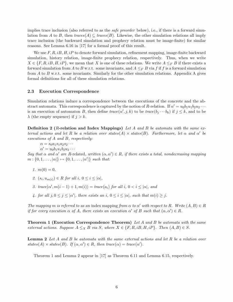
Simulation relations induce a correspondence between the executions of the concrete and the ab-stract automata. This correspondence is captured by the notion of R-relation. If α′ = u0b1u1b2u2 · · ·is an execution of automaton B, then define trace(α′, j, k) to be trace(bj · · · bk) if j ≤ k, and to beλ (the empty sequence) if j > k.

Definition 2 (R-relation and Index Mappings) Let A and B be automata with the same ex-ternal actions and let R be a relation over states(A) × states(B). Furthermore, let α and α′ beexecutions of A and B, respectively:

α = s0a1s1a2s2 · · ·α′ = u0b1u1b2u2 · · ·

Say that α and α′ are R-related, written (α,α′) ∈ R, if there exists a total, nondecreasing mappingm : {0, 1, . . . , |α|} 7→ {0, 1, . . . , |α′|} such that:

1. m(0) = 0,

2. (si, um(i)) ∈ R for all i, 0 ≤ i ≤ |α|,

3. trace(α′,m(i− 1) + 1,m(i)) = trace(ai) for all i, 0 < i ≤ |α|, and

4. for all j, 0 ≤ j ≤ |α′|, there exists an i, 0 ≤ i ≤ |α|, such that m(i) ≥ j.

The mapping m is referred to as an index mapping from α to α′ with respect to R. Write (A,B) ∈ Rif for every execution α of A, there exists an execution α′ of B such that (α,α′) ∈ R.

Theorem 1 (Execution Correspondence Theorem) Let A and B be automata with the sameexternal actions. Suppose A ≤X B via S, where X ∈ {F,R, iB,H, iP}. Then (A,B) ∈ S.

Lemma 2 Let A and B be automata with the same external actions and let R be a relation overstates(A) × states(B). If (α,α′) ∈ R, then trace(α) = trace(α′).

Theorem 1 and Lemma 2 appear in [17] as Theorem 6.11 and Lemma 6.15, respectively.

6

2.4 Linear-time Temporal Logic

We use the fragment of linear-time temporal logic consisting of the 2 (always) and 3 (eventually)operators over state assertions [47, 39]. In particular, we use the “infinitary” operators 23 (in-finitely often) and 32 (eventually always). We specify state assertions as a set of states, the statein question satisfying the assertion iff it belongs to the set.

For example, if U is a set of states, then α |= 23U means “α contains infinitely many states fromU ,” and α |= 32U means “all but a finite number of states of α are from U .” These operators canbe combined with propositional connectives (¬,∧,∨,⇒) so that, for example, α |= 23U ′ ⇒ 23U ′′

means “if α contains infinitely many states from U ′, then it also contains infinitely many statesfrom U ′′, and α |= 32¬U means “all but a finite number of states of α are not from U .”

Appendix B provides a formal definition of the syntax and semantics of the temporal logic thatwe use.

3 Live Automata

We first formalize the notions of live execution property and live trace property, that discussed inthe introduction.

Definition 3 (Live Execution Property) Let A be an automaton, and ϕ ⊆ execsω(A). Then,ϕ is a live execution property for A if and only if for every finite execution α of A, there exists aninfinite execution α′ of A such that α < α′ and α′ ∈ ϕ.

In other words, a live execution property is a set of infinite executions of A such that every finiteexecution of A can be extended to an infinite execution in the set. This requirement was proposedin [1], where it is called machine closure.

Note that we do not consider interaction with an environment in this paper. THis is why weuse automata rather than I/O automata, i.e., we have external actions without an input/outputdistinction. This issue is treated in detail in [18], where a liveness property is defined as a set ofexecutions (finite or infinite) such that any finite execution can be extended to an execution in theset. Thus, an extension may be finite, unlike our approach. This is because requiring extensionto an infinite execution may constrain the environment: an execution ending in a state with noenabled internal or output action will then require the environment to execute an action that is anoutput of the environment and an input of the automaton, so that the execution can be extendedto an infinite one. We defer treating this issue to another occasion.

Definition 4 (Live Trace Property) Let A be an automaton, and ψ ⊆ traces(A). Then, ψ isa live trace property for A if and only if there exists a live execution property ϕ for A such thatψ = traces(ϕ).

In [17, 18], the notion of live execution property was the basic liveness notion, and a liveautomaton was defined to be an automaton A together with a live execution property. This use ofan arbitrary set of executions as a liveness property, subject only to the machine closure constraintresulted in a proof method in [17] which requires reasoning over entire executions. Since we wishto avoid this, we take as our basic liveness notion the complemented-pairs condition of Streett

7

automata, with the proviso that we extend it to an infinite state-space and an infinite number ofcomplemented-pairs. In the next section, we show that this approach to specifying liveness entailsno loss of expressiveness, provided that we can use history variables.

Let A be an automaton. We say that p is a complemented-pair3 over A iff p is an orderedpair 〈〈〈Red,Green〉〉〉 where Red ⊆ states(A), Green ⊆ states(A). Given p = 〈〈〈Red,Green〉〉〉, we definethe selectors p.R = Red and p.G = Green. Let α be an infinite execution of A. Then, we writeα |= 〈〈〈Red,Green〉〉〉 iff α |= 23Red ⇒ 23Green, i.e., if α contains infinitely many states in Red, thenit also contains infinitely many states in Green. We also write α |= p in this case. Our goal is amethod for refining liveness properties using reasoning over states and finite execution fragmentsonly, in particular, avoiding reasoning over entire (infinite) executions. We therefore formulate aliveness condition based on states rather than executions.

Definition 5 (Live Automaton with Complemented-pairs Liveness Condition) A live au-tomaton is a pair (A,L) where:

1. A is an automaton, and

2. L is a set of pairs {〈〈〈RediA,Greeni

A〉〉〉 | i ∈ η} where RediA ⊆ states(A) and Greeni

A ⊆ states(A)for all i ∈ η, and η is some cardinal, which serves as an index set,

and A, L satisfy the following constraint:

• for every finite execution α of A, there exists an infinite execution α′ of A such that

α < α′ and (∀p ∈ L : α′ |= p).

(A,L) inherits all of the attributes of A, namely the states, start states, action signature, and tran-sition relation of A. The executions (execution fragments) of (A,L) are the executions (executionfragments) of A, respectively. We say that L is a complemented-pairs liveness condition over A.Often we use just “liveness condition” instead of “complemented-pairs liveness condition.”

The constraint in Definition 5 is the machine closure requirement, that every finite executioncan be extended to a live execution.

Definition 6 (Live Execution) Let (A,L) be a live automaton. An execution α of (A,L) is alive execution iff α is infinite and ∀p ∈ L : α |= p.We define lexecs(A,L) = {α | α ∈ execsω(A) and (∀p ∈ L : α |= p)}.

Our notion of liveness condition is essentially the acceptance condition for finite-state complemented-pairs automata on infinite strings [13], with the important difference that we generalize it to anarbitrary (possibly infinite) state space, and allow a possibly infinite set of pairs. Despite the pos-sibility that Redi

A and GreeniA are infinite sets of states, it is nevertheless very convenient to have

an infinite number of complemented-pairs. Using the database example of the introduction, we canexpress the liveness property “every query submitted is eventually processed” as the infinite setof pairs {〈〈〈x ∈ wait , x 6∈ wait〉〉〉 | x is a query}, and where wait is the set of all queries that havebeen submitted but not yet processed (x is removed from wait when it is processed). Being able

3When it is clear from context, we just say “pair”.

8

to allocate one pair for each query facilitates the very straightforward expression of this livenessproperty. Our extended example in Section 6 also uses an infinite number of pairs in this manner.

The above discussion applies to any system in which there are an infinite number of distinguishedoperations, e.g., each operation has a unique identifier, as opposed to, for example mutual exclusionfor a fixed finite number of processes,, where there are an infinite number of entries into the criticalsection by some process Pi, but these need not be “distinguished,” since the single liveness property2(request(Pi) =⇒ 3critical(Pi)) is sufficient to account for all of these. The key point is thatonly a bounded number of outstanding requests must be dealt with (≤ the number of processes) ,whereas in a system in which there are an infinite number of distinguished operations, an unboundednumber of outstanding requests must be dealt with. We conjecture that the liveness property “everyrequest is eventually satisfied” cannot even be stated using a finite number of complemented pairs.

The safe preorder, live preorder [17] embody our notions of correct implementation with respectto safety, liveness, respectively.

Definition 7 (Safe preorder, Live preorder) Let (A,L), (B,M) be live automata with thesame external actions (ext(A) = ext(B)). We define:

Safe preorder: (A,L) ⊑s (B,M) iff traces(A) ⊆ traces(B)

Live preorder: (A,L) ⊑ℓ (B,M) iff traces(lexecs(A,L)) ⊆ traces(lexecs(B,M))

From [34, 17], we have that simulation relations imply the safe preorder, i.e., if A ≤X B whereX ∈ {F,R, iB,H, iP}, then (A,L) ⊑s (B,M).

Returning to the database example of the introduction, if α is some live execution of theimplementation A, then, along α, every continuously enabled action is eventually executed (actionfairness) and every message sent is eventually received (message fairness). The trace β of α is thenan externally visible live behavior of A: β ∈ traces(lexecs(A,L)). If A is a correct implementation,then we expect that the enforcement of action fairness and message fairness in A then guaranteesthe required liveness properties of the specification, namely that every query is eventually processed.Thus, the externally visible live behavior β of A must satisfy the required liveness properties of thespecification, i.e., β ∈ traces(lexecs(B,M)). This is exactly what the live preorder requires.

Definition 8 (Semantic Closure of a Liveness Condition) Let (A,L) be a live automaton.The semantic closure L̂ of L in A is given by L̂ = {〈〈〈R,G〉〉〉 | ∀α ∈ lexecs(A,L) : α |= 〈〈〈R,G〉〉〉}.

L̂ is the set of complemented-pairs over A which are “semantically entailed” by the complemented-pairs in L, with respect to the executions of A. In general, L̂−L is nonempty. Every pair in L̂−Lrepresents a “derived” liveness property, since it is not directly specified by L, but nevertheless canbe deduced from the pairs in L, when considering only the executions of A.

Definition 9 (Derived Pair) Let (A,L) be a live automaton, and let p ∈ L̂ − L. Then p is aderived pair of (A,L).

Proposition 3 L ⊆ L̂.

Proof. Let p be any complemented-pair in L. Hence, by definition of lexecs(A,L), we have ∀α ∈lexecs(A,L) : α |= p. Hence p ∈ L̂. 2

9

Proposition 4 lexecs(A, L̂) = lexecs(A,L).

Proof. lexecs(A, L̂) ⊆ lexecs(A,L) follows immediately from Proposition 3 and the relevant defini-tions. Suppose α ∈ lexecs(A,L). By Definition 8, ∀p ∈ L̂ : α |= p. Hence, α ∈ lexecs(A, L̂). Hencelexecs(A,L) ⊆ lexecs(A, L̂). 2

From Proposition 4, it follows that (A, L̂) is a live automaton.

4 Refining Liveness Properties Across Levels of Abstraction: Liveness-

preserving Simulation Relations

The simulation relations given in Section 2.2 induce a relationship between the concrete automatonA and abstract automaton B whereby for every execution α of A there exists a corresponding,in the sense of Definition 2, execution α′ of B. This correspondence between executions does nothowever take liveness into account. So, if we were dealing with live automata (A,L) and (B,M) in-stead of automata A and B, then it would be possible to have α ∈ lexecs(A,L), α′ 6∈ lexecs(B,M),and (α,α′) ∈ S where S is a simulation relation from A to B. So, β ∈ traces(lexecs(A,L)) andβ /∈ traces(lexecs(B,M)), where β = trace(α), is possible. Hence establishing A ≤X B via S, whereX ∈ {F,R, iB,H, iP} does not allow one to conclude traces(lexecs(A,L)) ⊆ traces(lexecs(B,M)),as desired, whereas it does allow one to conclude traces(A) ⊆ traces(B), [17, Lemma 6.16]. Forexample, consider Figures 1 and 2 which respectively give a specification and a “first level” refine-ment of the specification, for a toy database system. The database takes input requests of the formrequest(x), where x is a query, computes a response for x using a function val (which presumablyalso refers to the underlying database state, we do not model this to keep the example simple),and outputs a response (x, v) where v = val(x). This behavior is dictated by the specificationin Figure 1, where received queries are placed in the set requested , and queries responded to areplaced in the set responded (this prevents multiple responses to the same query). The first-levelrefinement of the specification (Figure 2) is identical to the specification except that it can “lose”pending requests: the request(x) nondeterministically chooses between adding x to requested , ordoing nothing, as represented by []skip in Figure 2. Despite this fault, it is possible to establish aforward simulation F from DB-Imp to DB-Spec, as follows. A state s of DB-Imp and a state u ofDB-Spec are related by F if and only if s.requested ⊆ u.requested and s.responded = u.responded(where s.var denotes the value of variable var in state s). Now suppose we add the following live-ness condition to both DB-Imp and of DB-Spec: {〈〈〈x ∈ requested , x ∈ responded 〉〉〉 | x is a query}.Thus, an operation x that has been requested must eventually be responded to, since x ∈ requestedis stable; once true, it is always true, and therefore it is true infinitely often. Now let α, α′ beexecutions of DB-Imp, DB-Spec, respectively, which are related by F in the sense of Definition 2.Suppose some query x0 is lost along α, and no other query is lost. Let α be live, i.e., if a query isplaced into requested , and is not lost, then it will eventually be responded to. We now see that α′

cannot be live, since x0 ∈ requested holds along an infinite suffix of α′, but x0 ∈ responded neverholds along α′. Hence, establishing a forward simulation from DB-Imp to DB-Spec is not sufficientto establish live trace inclusion from DB-Imp to DB-Spec.

This example demonstrates that the simulation relations of Section 2.2 do not imply live traceinclusion. The problem is that these simulation relations do not reference the liveness conditionsof the concrete and abstract automata. To remedy this, we augment the simulation relations sothat every pair q in the abstract liveness condition M is related to a pair p in the concrete livenesscondition L. The idea is that the simulation relation relates occurrences of states in q.R, q.G in

10

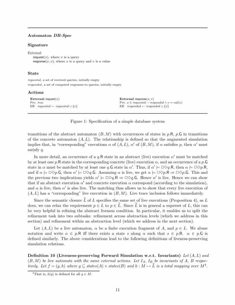
Automaton DB-Spec

Signature

External:request(x), where x is a queryresponse(x, v), where x is a query and v is a value

State

requested , a set of received queries, initially empty

responded , a set of computed responses to queries, initially empty

Actions

External request(x)Pre: true

Eff: requested ← requested ∪ {x}

External response(x, v)Pre: x ∈ requested − responded ∧ v = val(x)Eff: responded ← responded ∪ {x}

Figure 1: Specification of a simple database system

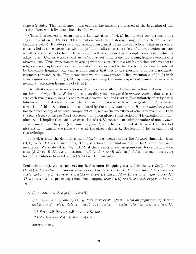
transitions of the abstract automaton (B,M) with occurrences of states in p.R, p.G in transitionsof the concrete automaton (A,L). The relationship is defined so that the augmented simulationimplies that, in “corresponding” executions α of (A,L), α′ of (B,M), if α satisfies p, then α′ mustsatisfy q.

In more detail, an occurrence of a q.R state in an abstract (live) execution α′ must be matchedby at least one p.R state in the corresponding concrete (live) execution α, and an occurrence of a p.Gstate in α must be matched by at least one q.G state in α′. Thus, if α′ |= 23q.R, then α |= 23p.R,and if α |= 23p.G, then α′ |= 23q.G. Assuming α is live, we get α |= 23p.R ⇒ 23p.G. This andthe previous two implications yields α′ |= 23q.R ⇒ 23q.G. Hence α′ is live. Hence we can showthat if an abstract execution α′ and concrete execution α correspond (according to the simulation),and α is live, then α′ is also live. The matching thus allows us to show that every live execution of(A,L) has a “corresponding” live execution in (B,M). Live trace inclusion follows immediately.

Since the semantic closure L̂ of L specifies the same set of live executions (Proposition 4), as Ldoes, we can relax the requirement p ∈ L to p ∈ L̂. Since L̂ is in general a superset of L, this canbe very helpful in refining the abstract liveness condition. In particular, it enables us to split therefinement task into two subtasks: refinement across abstraction levels (which we address in thissection) and refinement within an abstraction level (which we address in the next section).

Let (A,L) be a live automaton, α be a finite execution fragment of A, and p ∈ L. We abusenotation and write α ∈ p.R iff there exists a state s along α such that s ∈ p.R. α ∈ p.G isdefined similarly. The above considerations lead to the following definitions of liveness-preservingsimulation relations.

Definition 10 (Liveness-preserving Forward Simulation w.r.t. Invariants) Let (A,L) and(B,M) be live automata with the same external actions. Let IA, IB be invariants of A, B respec-tively. Let f = (g, h) where g ⊆ states(A)× states(B) and h : M 7→ L̂ is a total mapping over M4.

4That is, h(q) is defined for all q ∈ M .

11

Automaton DB-Imp

Signature

External:request(x), where x is a queryresponse(x, v), where x is a query and v is a value

State

requested , a set of received queries, initially empty

responded , a set of computed responses to queries, initially empty

Actions

External request(x)Pre: true

Eff: (requested ← requested ∪ {x}) [] skip

External response(x, v)Pre: x ∈ requested − responded ∧ v = val(x)Eff: responded ← responded ∪ {x}

Figure 2: First level refinement of the specification of a simple database system

Then f is a liveness-preserving forward simulation from (A,L) to (B,M) with respect to IA andIB iff:

1. If s ∈ start(A), then g[s] ∩ start(B) 6= ∅.

2. If sa

−→A s′, s ∈ IA, and u ∈ g[s] ∩ IB, then there exists a finite execution fragment α of

B such that fstate(α) = u, lstate(α) ∈ g[s′], and trace(α) = trace(a). Furthermore, for allq ∈M ,

(a) if α ∈ q.R then s ∈ p.R or s′ ∈ p.R, and

(b) if s ∈ p.G or s′ ∈ p.G then α ∈ q.G,

where p = h(q).

3. Call a transition sa

−→A s′ always-silent iff s ∈ IA and for every finite execution fragment α of

B such that fstate(α) ∈ g[s] ∩ IB, lstate(α) ∈ g[s′], and trace(α) = trace(a), we have |α| = 0,i.e., α consists of a single state. In other words, the transition s

a−→A s

′ is matched only bythe empty transition in B. Then, g is such that every live execution of (A,L) contains aninfinite number of transitions that are not always-silent.

Clause 1 is the usual condition of a forward simulation requiring that every start state of (A,L)be related to at least one start state of (B,M).

Clause 2 is the condition of a forward simulation which requires that every transition sa

−→A s′

of (A,L) be “simulated” by an execution fragment α of (B,M) which has the same trace. We alsorequire that every complemented-pair q ∈ M is matched to a complemented-pair p ∈ L̂ by themapping h and that such corresponding pairs impose a constraint on the transition s

a−→A s

′ of(A,L) and the simulating execution fragment α of (B,M), as follows. If α contains some q.R state,then at least one of s, s′ is a p.R state, and if at least one of s, s′ is a p.G state, then α contains

12

some q.G state. This requirement thus enforces the matching discussed at the beginning of thissection, from which live trace inclusion follows.

Clause 3 is needed to ensure that a live execution of (A,L) has at least one correspondinginfinite execution in (B,M). This execution can then be shown, using clause 2, to be live (seeLemma 8 below). If s

a−→A s

′ is always-silent, then a must be an internal action. Thus, in practice,clause 3 holds, since executions with an (infinite) suffix consisting solely of internal actions are notusually considered to be live. Clause 3 can itself be expressed as a complemented-pair (which isadded to L). Call an action a of A non-always-silent iff no transition arising from its execution isalways-silent. Thus, every transition arising from the execution of a can be matched with respect tog by some nonempty execution fragment of B. It is also possible that the transition can be matchedby the empty fragment, but what is important is that it is always possible to choose a nonemptyfragment to match with. This means that we can always match a live execution α of (A,L) withsome infinite execution of (B,M), by always matching the non-always-silent transitions in α withnonempty execution fragments of (B,M).

By definition, any external action of A is non-always-silent. An internal action of A may or maynot be non-always-silent. We introduce an auxiliary boolean variable nonalwayssilent that is set totrue each time a non-always-silent action of A is executed, and is set to false infinitely often by a newinternal action of A whose precondition is true and whose effect is nonalwayssilent := false (everyexecution of this new action can be simulated by the empty transition in B, since nonalwayssilenthas no effect on any other state component of A, nor on the execution of other actions in A). Thenthe pair 〈〈〈true ,nonalwayssilent 〉〉〉 expresses that a non-always-silent action of A is executed infinitelyoften, which implies that each live execution of (A,L) contains an infinite number of non-always-silent transitions. The pair 〈〈〈true ,nonalwayssilent 〉〉〉 can then be refined at the next lower level ofabstraction in exactly the same way as all the other pairs in L. See Section 6 for an example ofthis technique.

It is clear from the definitions that if (g, h) is a liveness-preserving forward simulation from(A,L) to (B,M) w.r.t. invariants, then g is a forward simulation from A to B w.r.t. the sameinvariants. We write (A,L) ≤ℓF (B,M) if there exists a liveness-preserving forward simulationfrom (A,L) to (B,M) w.r.t. invariants, and (A,L) ≤ℓF (B,M) via f if f is a liveness-preservingforward simulation from (A,L) to (B,M) w.r.t. invariants.

Definition 11 (Liveness-preserving Refinement Mapping w.r.t. Invariants) Let (A,L) and(B,M) be live automata with the same external actions. Let IA, IB be invariants of A, B, respec-tively. Let r = (g, h) where g : states(A) 7→ states(B) and h : M 7→ L̂ is a total mapping over M .Then r is a liveness-preserving refinement mapping from (A,L) to (B,M) with respect to IA andIB iff:

1. If s ∈ start(A), then g(s) ∈ start(B).

2. If sa

−→A s′, s ∈ IA, and g(s) ∈ IB, then there exists a finite execution fragment α of B such

that fstate(α) = g(s), lstate(α) = g(s′), and trace(α) = trace(a). Furthermore, for all q ∈M ,

(a) if α ∈ q.R then s ∈ p.R or s′ ∈ p.R, and

(b) if s ∈ p.G or s′ ∈ p.G then α ∈ q.G,

where p = h(q).

13

3. Call a transition sa

−→A s′ always-silent iff s ∈ IA and for every finite execution fragment α

of B such that fstate(α) = g(s), lstate(α) = g(s′), and trace(α) = trace(a), we have |α| = 0,i.e., α consists of a single state. In other words, the transition s

a−→A s

′ is matched only bythe empty transition in B. Then, g is such that every live execution of (A,L) contains aninfinite number of transitions that are not always-silent.

We write A ≤ℓR B if there exists a liveness-preserving refinement mapping from A to B w.r.t.invariants, and A ≤ℓR B via r if r is a liveness-preserving refinement mapping from A to B w.r.t.invariants. It is clear from the definitions that a liveness-preserving refinement mapping is a specialcase of a liveness-preserving forward simulation. Furthermore, if (g, h) is a liveness-preservingrefinement mapping from (A,L) to (B,M) w.r.t. some invariants, then g is a refinement mappingfrom A to B w.r.t. the same invariants.

Definition 12 (Liveness-preserving Backward Simulation w.r.t. Invariants) Let (A,L) and(B,M) be live automata with the same external actions. Let IA, IB be invariants of A, B respec-tively. Let b = (g, h) where g ⊆ states(A) × states(B) and h : M 7→ L̂ is a total mapping over M .Then b is a liveness-preserving backward simulation from (A,L) to (B,M) with respect to IA andIB iff:

1. If s ∈ IA, then g[s] ∩ IB 6= ∅.

2. If s ∈ start(A), then g[s] ∩ IB ⊆ start(B).

3. If sa

−→A s′, s ∈ IA, and u′ ∈ g[s′] ∩ IB, then there exists a finite execution fragment α of B

such that fstate(α) ∈ g[s] ∩ IB, lstate(α) = u′, and trace(α) = trace(a). Furthermore, for allq ∈M ,

(a) if α ∈ q.R then s ∈ p.R or s′ ∈ p.R, and

(b) if s ∈ p.G or s′ ∈ p.G then α ∈ q.G,

where p = h(q).

4. Call a transition sa

−→A s′ sometimes-silent iff s ∈ IA and for some finite execution fragment

α of B such that fstate(α) ∈ g[s] ∩ IB, lstate(α) ∈ g[s′], and trace(α) = trace(a), we have|α| = 0, i.e., α consists of a single state. In other words, the transition s

a−→A s

′ can bematched by the empty transition in B. Then, g is such that every live execution of (A,L)contains an infinite number of transitions that are not sometimes-silent.

Clauses 1 and 2 are the usual conditions of a backward simulation requiring that a state in theinvariant IA of (A,L) is related to at least one state in the invariant IB of (B,M), and that everystart state of (A,L) is related only to start states of (B,M), ignoring states not in the invariant IB .These clauses are needed due to the “backwards” nature of the bisimulation, since, from a stateu′ in the invariant IB it is possible, when “going backwards” along a transition to reach a state unot in the invariant, i.e., u

a−→B u

′, u /∈ IB , and u′ ∈ IB is possible. Also, a start state in (A,L)must always be matched by a start state in (B,M), since the matching state in (B,M) cannot bechosen initially: it is constrained by the succeeding transitions, i.e., it is “chosen” last of all, andso the result must be an initial state of B regardless of the choice.

Clause 3 is the condition of a backward simulation which requires that every transition sa

−→A s′

of (A,L) be “simulated” by an execution fragment α of (B,M), except that we also require that

14

every complemented-pair q ∈ M is matched to a complemented-pair p ∈ L̂ by the mapping h andthat such corresponding pairs impose a constraint on the transition s

a−→A s

′ of (A,L) and thesimulating execution fragment α of (B,M), as follows. If α contains some q.R state, then at leastone of s, s′ is a p.R state, and if at least one of s, s′ is a p.G state, then α contains some q.G state.This requirement thus enforces the matching discussed at the beginning of this section, from whichlive trace inclusion follows.

Clause 4 is needed to ensure that a live execution of (A,L) has at least one corresponding infiniteexecution in (B,M). This execution can then be shown, using clause 3, to be live (see Lemma 8below). If s

a−→A s

′ is sometimes-silent, then a must be an internal action. Thus, in practice,clause 4 holds, since executions with an (infinite) suffix consisting solely of internal actions are notusually considered to be live. Clause 4 can itself be expressed as a complemented-pair (which isadded to L), which can then be refined at the next lower level of abstraction. Call an action aof A non-sometimes-silent iff no transition arising from its execution is sometimes-silent. Thus,every transition arising from the execution of a must always be matched with respect to g by somenonempty execution fragment of B.

We can now express the requirement that a non-sometimes-silent action of A is executed in-finitely often, as a complemented-pair, and refine this pair at the next lower level of abstraction.The details are similar to those discussed above for Clause 3 of Definition 10, and are omitted.Note the difference with forward simulation; there, we only had to ensure that it was infinitely of-ten possible to choose a nonempty execution fragment to match with. With backward simulations,we have to show that infinitely often, all the matching execution fragments are nonempty.

It is clear from the definitions that if (g, h) is a liveness-preserving backward simulation from(A,L) to (B,M) w.r.t. some invariants, then g is a backward simulation from A to B w.r.t. thesame invariants. We write A ≤ℓB B if there exists a liveness-preserving backward simulation fromA to B w.r.t. some invariants, and A ≤ℓB B via b if b is a liveness-preserving backward simulationfrom A to B w.r.t. some invariants. If the backward simulation g is image-finite, then we writeA ≤iℓB B, A ≤iℓB B via b, respectively.

Definition 13 (Liveness-preserving History Relation w.r.t. Invariants) Let (A,L) and(B,M) be live automata with the same external actions. Let IA, IB be invariants of A, B,respectively. A history relation from A to B with respect to IA and IB is a relation hs overstates(A) × states(B) that satisfies:

1. hs is a liveness-preserving forward simulation from A to B w.r.t. IA and IB, and

2. hs−1 is a refinement from B to A w.r.t. IB and IA.

We write A ≤ℓH B if there exists a liveness-preserving history relation from A to B w.r.t. someinvariants, and A ≤ℓH B via h if h is a liveness-preserving history relation from A to B w.r.t. someinvariants.

Definition 14 (Liveness-preserving Prophecy Relation w.r.t. Invariants) Let (A,L) and(B,M) be live automata with the same external actions. Let IA, IB be invariants of A, B, re-spectively. A prophecy relation from A to B with respect to IA and IB is a relation p overstates(A) × states(B) that satisfies:

1. p is a liveness-preserving backward simulation from A to B w.r.t. IA and IB, and

15

2. p−1 is a refinement from B to A w.r.t. IB and IA.

We write A ≤ℓP B if there exists a liveness-preserving prophecy relation from A to B w.r.t. someinvariants, and A ≤ℓP B via p if p is a liveness-preserving prophecy relation from A to B w.r.t. someinvariants. If the liveness-preserving prophecy relation is image-finite, then we write A ≤iℓP B,A ≤iℓP B via p, respectively.

We use ℓF, ℓR, iℓB, ℓH, iℓP to denote liveness-preserving forward simulation, liveness-preservingrefinement mapping, image-finite liveness-preserving backward simulation, liveness-preserving his-tory relation, image-finite liveness-preserving prophecy relation, respectively. Thus, when we writeX ∈ {ℓF, ℓR, iℓB, ℓH, iℓP}, we mean that X is one of these relations.

Liveness-preserving simulation relations induce a correspondence between the live executionsof the concrete and the abstract automata. This correspondence is captured by the notion of Rℓ-relation. We remind the reader of the definition trace(α′, j, k) = trace(bj · · · bk) if j ≤ k, and = λ(the empty sequence) if j > k.

Definition 15 (Rℓ-relation and Live Index Mappings) Let (A,L) and (B,M) be live automatawith the same external actions. Let Rℓ = (R,H) where R is a relation over states(A) × states(B)and H : M 7→ L̂ is a total mapping over M . Furthermore, let α and α′ be executions of (A,L) and(B,M), respectively:

α = s0a1s1a2s2 · · ·α′ = u0b1u1b2u2 · · ·

Say that α and α′ are Rℓ-related, written (α,α′) ∈ Rℓ, if there exists a total, nondecreasing mappingm : {0, 1, . . . , |α|} 7→ {0, 1, . . . , |α′|} such that:

1. m(0) = 0,

2. (si, um(i)) ∈ R for all i, 0 ≤ i ≤ |α|,

3. trace(α′,m(i− 1) + 1,m(i)) = trace(ai) for all i, 0 < i ≤ |α|,

4. for all j, 0 ≤ j ≤ |α′|, there exists an i, 0 ≤ i ≤ |α|, such that m(i) ≥ j, and

5. for all complemented-pairs q ∈M and all i, 0 < i ≤ |α| :

(a) if (∃j ∈ m(i− 1) . . . m(i) : uj ∈ q.R) then si−1 ∈ p.R or si ∈ p.R, and

(b) if si−1 ∈ p.G or si ∈ p.G then (∃j ∈ m(i− 1) . . . m(i) : uj ∈ q.G),

where p = H(q).

The mapping m is referred to as a live index mapping from α to α′ with respect to Rℓ. Write((A,L), (B,M)) ∈ Rℓ if for every live execution α of (A,L), there exists a live execution α′ of(B,M) such that (α,α′) ∈ Rℓ.

Note that (α,α′) ∈ Rℓ does not require α,α′ to be live executions. By Definitions 2 and 15, it isclear that, if Rℓ = (R,H), then (α,α′) ∈ Rℓ implies (α,α′) ∈ R. The following lemma establishes acorrespondence between the prefixes of a live execution of the concrete automaton and an infinitefamily of finite executions of the abstract automaton.

16

Lemma 5 Let (A,L) and (B,M) be live automata with the same external actions, and such that(A,L) ≤ℓF (B,M) via f for some f = (g, h). Let α be an arbitrary live execution of (A,L). Thenthere exists a collection (α′i,mi)0≤i of finite executions of (B,M) and mappings such that:

1. mi is a live index mapping from α|i to α′i with respect to f , for all i ≥ 0, and

2. α′i−1 ≤ α′i and mi−1 = mi↾{0, . . . , i− 1} for all i > 0, and

3. α′i−1 < α′i for infinitely many i > 0.

Proof. Let α = s0a1s1a2s2 . . . and let IA, IB be invariants of A, B, respectively, such that f isa liveness-preserving forward simulation from (A,L) to (B,M) with respect to IA and IB . Weconstruct α′i and mi by induction on i.

Since s0 ∈ start(A), we have (s0, v0) ∈ g and v0 ∈ start(B) for some state v0, by Definition 10,clause 1. Let α′0 = v0 and let m0 be the mapping that maps 0 to 0. Then, m0 is a live indexmapping from α|0 to α′0 with respect to f (in particular, clause 5 of Definition 15 holds vacuously,since |α|0| = 0).

Now inductively assume that mi−1 (for i > 0) is a live index mapping from α|i−1 to α′i−1 withrespect to f . Let u0 = lstate(α′i−1). Then, by clause 4 of Definition 15 and the fact that mi−1

is nondecreasing, we have mi−1(i − 1) = |α′i−1| and (si−1, u0) ∈ g. Since si−1, si, and u0 arereachable, by definition, they satisfy their respective invariants. Hence, by Definition 10, clause 2,

there exists a finite execution fragment u0b1−→B u1

b2−→B · · ·bn−→B un of B such that un ∈ g[si],

trace(b1 · · · bn) = trace(ai), and for all complemented-pairs q ∈M :

1. if (∃j ∈ 1 . . . n : uj ∈ q.R) then si−1 ∈ p.R or si ∈ p.R, and

2. if si−1 ∈ p.G or si ∈ p.G then (∃j ∈ 1 . . . n : uj ∈ q.G),

where p = h(q). Now define α′i = α′i−1⌢(u0

b1−→B u1b2−→B · · ·

bn−→B un), and define mi to be themapping such that mi(j) = mi−1(j) for all j, 0 ≤ j ≤ i− 1, and mi(i) = |α′i|. We argue that mi isa live index mapping from α|i to α′i with respect to f , i.e., that all clauses of Definition 15 hold.Clause 1 holds since mi(0) = mi−1(0) by definition, and mi−1(0) = 0 by the inductive hypothesis.Clause 2 holds by the inductive hypothesis and un ∈ g[si]. Clause 3 holds by the inductive hypoth-esis and trace(b1 · · · bn) = trace(ai). Clause 4 holds since mi(|α|i |) = mi(i) = |α′i|, by definition.Finally, clause 5 holds by the inductive hypothesis and the conditions for all complemented-pairs

q ∈ M just established above w.r.t. si−1ai−→A si and u0

b1−→B u1b2−→B · · ·

bn−→B un. Having estab-lished that mi is a live index mapping from α|i to α′i with respect to f , we conclude that clause 1of the lemma holds.

Clause 2 of the lemma holds by construction of α′i and mi, since α′i and mi are obtained byextending α′i−1 and mi−1, respectively.

By Definition 10, clause 3, for infinitely many i > 0, we can select the execution fragment

u0b1−→B u1

b2−→B · · ·bn−→B un that matches si−1

ai−→A si so that n > 0. Hence, for infinitely manyi > 0, we have α′i−1 < α′i. Thus, clause 3 of the lemma holds. 2

Definition 16 (Induced Digraph) Let (A,L) and (B,M) be live automata with the same ex-ternal actions and assume A ≤iℓB B via b = (g, h) with respect to invariants IA and IB. For anyexecution α = s0a1s1a2s2 . . . of A, let the digraph induced by α, b, IB, L, and M be the directedgraph G given as follows:

17

1. The nodes of G are the ordered pairs (u, i) such that 0 ≤ i ≤ |α|, and u ∈ g[si] ∩ IB, and

2. there is an edge from (u, i) to (u′, i′) iff i′ = i + 1 and there exists a finite execution frag-ment α′ of B such that fstate(α′) = u, lstate(α′) = u′, trace(α′) = trace(ai+1), and for allcomplemented-pairs q ∈M :

(a) if α′ ∈ q.R then si ∈ p.R or si+1 ∈ p.R, and

(b) if si ∈ p.G or si+1 ∈ p.G then α′ ∈ q.G,

where p = h(q).

Lemma 6 Let (A,L) and (B,M) be live automata with the same external actions and assumeA ≤iℓB B via b with respect to invariants IA and IB. Let α be any execution of A. Then thedigraph G induced by α, b, IB, L, and M satisfies:

1. For each i, 0 ≤ i ≤ |α|, there is at least one node in G of the form (u, i).

2. The roots of G are exactly the nodes of the form (u, 0).

3. G has a finite number of roots.

4. Each node in G has finite outdegree.

5. Each node of G is reachable from some root of G.

Proof. Let b = (g, h). Then g is an image-finite backward simulation from A to B. We deal witheach clause in turn.

1. Each state si of α is reachable, and so belongs to IA. Hence g[si] ∩ IB 6= ∅ by Clause 1 ofDefinition 12. Hence by Definition 16, clause 1, there exist nodes of G of the form (u, i).

2. Every node (u, 0) is a root of G (i.e., it has no incoming edges). We now show that anynode (u, i) with i > 0 cannot be a root. Now u ∈ g[si] ∩ IB by Definition 16, clause 1.

Also, si−1 ∈ IA and si−1ai−→A si by assumption, hence by Definition 12, clause 3, there

exists a finite execution fragment α′ of B such that fstate(α′) ∈ g[si−1] ∩ IB, lstate(α′) = u,trace(α′) = trace(ai), and, for all q ∈M ,

(a) if α′ ∈ q.R then si−1 ∈ p.R or si ∈ p.R, and

(b) if si−1 ∈ p.G or si ∈ p.G then α′ ∈ q.G,

where p = h(q). Hence, by Definition 16, clause 2, there exists an edge inG from (fstate(α′), i−1) to (u, i).

3. Since g is image-finite, the set g[s0] ∩ IB is finite. By Definition 16, clause 1, all nodes of Gof the form (u, 0) must satisfy u ∈ g[s0]∩ IB. Hence, there are a finite number of such nodes.By clause 2 of the lemma (which has already been established), these nodes are exactly theroots of G. Hence, the number of roots is finite.

4. Let (u, i) be an arbitrary node of G. By Definition 16, clause 2, from any node of the form(u, i), all outgoing edges are to nodes of the form (u′, i + 1). Since g is image-finite, the setg[si+1] ∩ IB is finite. By Definition 16, clause 1, all nodes of G of the form (u, i + 1) mustsatisfy u ∈ g[si+1]∩ IB. Hence, there are a finite number of such nodes. Hence, the outdegreeof any node of G of the form (u, i) is finite. Since (u, i) was chosen arbitrarily, the resultfollows.

18

5. We establish this by induction on the second component i of the nodes (u, i) of G. For thebase case, i = 0 and nodes (u, 0) are reachable by definition since they are roots. Assume theinduction hypothesis that all nodes of the form (u, i) are reachable from some root of G, andconsider an arbitrary node of the form (u, i+ 1).

Now u ∈ g[si+1]∩IB by Definition 16, clause 1. Also, si ∈ IA and siai+1

−→A si+1 by assumption,hence by Definition 12, clause 3, there exists a finite execution fragment α′ of B such thatfstate(α′) ∈ g[si] ∩ IB , lstate(α′) = u, trace(α′) = trace(ai+1), and, for all q ∈M ,

(a) if α′ ∈ q.R then si ∈ p.R or si+1 ∈ p.R, and

(b) if si ∈ p.G or si+1 ∈ p.G then α′ ∈ q.G,

where p = h(q). Hence, by Definition 16, clause 2, there exists an edge in G from (fstate(α′), i)to (u, i + 1). By the induction hypothesis, (fstate(α′), i) is reachable. Hence, so is (u, i + 1).

Since all the clauses are established, Lemma 6 holds. 2

Lemma 7 Let (A,L) and (B,M) be live automata with the same external actions, and such that(A,L) ≤iℓB (B,M) via b for some b = (g, h). Let α be an arbitrary live execution of (A,L). Thenthere exists a collection (α′i,mi)0≤i of finite executions of (B,M) and mappings such that:

1. mi is a live index mapping from α|i to α′i with respect to b, for all i ≥ 0, and

2. α′i−1 ≤ α′i and mi−1 = mi↾{0, . . . , i− 1} for all i > 0, and

3. α′i−1 < α′i for infinitely many i > 0.

Proof. Let α = s0a1s1a2s2 . . . and let IA, IB be invariants of A, B, respectively, such that b is aimage-finite liveness-preserving backward simulation from (A,L) to (B,M) with respect to IA andIB . Let G be the digraph induced by α, b, IB , L and M . Since α is infinite (all live executions areinfinite, by Definition 5), G is infinite. Hence, by clauses 3 and 4 of Lemma 6, and Konig’s lemma,G contains an infinite path. Fix p = (u0, 0)(u1, 1), . . . to be any such path. By Definition 16,clause 1, ui ∈ g[si] ∩ IB for all i ≥ 0. We now construct α′i and mi by induction on i, with α′i suchthat lstate(α′i) = ui.

Now s0 ∈ start(A) since α is an execution of A. Also, by Definition 16, u0 ∈ g[s0] ∩ IB. Hence,by clause 2 of Definition 12, u0 ∈ start(B). Let α′0 = u0 and let m0 be the mapping that maps 0to 0. Then, m0 is a live index mapping from α|0 to α′0 with respect to b (in particular, clause 5 ofDefinition 15 holds vacuously, since |α|0| = 0), and lstate(α′0) = u0.

Now inductively assume that mi−1 (for i > 0) is a live index mapping from α|i−1 to α′i−1 withrespect to b, and that lstate(α′i−1) = ui−1. By construction of path p, there is an edge in G from(ui−1, i−1) to (ui, i). Hence, by Definition 16, there exists a finite execution fragment α′′ such thatfstate(α′′) = ui−1, lstate(α′′) = ui, trace(α′′) = trace(ai), and, for all complemented-pairs q ∈M :

1. if α′′ ∈ q.R then si−1 ∈ p.R or si ∈ p.R, and

2. if si−1 ∈ p.G or si ∈ p.G then α′′ ∈ q.G,

where p = h(q). Now define α′i = α′i−1⌢α′′, and define mi to be the mapping such that mi(j) =

mi−1(j) for all j, 0 ≤ j ≤ i− 1, and mi(i) = |α′i|. We argue that mi is a live index mapping from

19

α|i to α′i with respect to b, i.e., that all clauses of Definition 15 hold, and that lstate(α′i) = ui.Clause 1 holds since mi(0) = mi−1(0) by definition, and mi−1(0) = 0 by the inductive hypothesis.Clause 2 holds by the inductive hypothesis, lstate(α′′) = ui, and ui ∈ g[si] (which we establishedabove). Clause 3 holds by the inductive hypothesis and trace(α′′) = trace(ai). Clause 4 holds sincemi(|α|i |) = mi(i) = |α′i|, by definition. Finally, clause 5 holds by the inductive hypothesis and the

conditions for all complemented-pairs q ∈M established above w.r.t. si−1ai−→A si and α′′. Having

established that mi is a live index mapping from α|i to α′i with respect to f , we conclude thatclause 1 of the lemma holds. Also, lstate(α′i) = lstate(α′′) = ui, as required for the induction stepto be valid.

Clause 2 of the lemma holds by construction of α′i and mi, since α′i and mi are obtained byextending α′i−1 and mi−1, respectively.

By Definition 12, clause 4, for infinitely many i > 0, the execution fragment α′′ which matchessi−1

ai−→A si must have length |α′′| ≥ 1. Hence, for infinitely many i > 0, we have α′i−1 < α′i. Thus,clause 3 of the lemma holds. 2

Our next lemma shows that, if infinite concrete and abstract executions correspond in the senseof (α,α′) ∈ Rℓ, and the concrete execution is live, then so is the abstract execution.

Lemma 8 Let (A,L) and (B,M) be live automata with the same external actions. Let Rℓ =(R,H) where R is a relation over states(A) × states(B) and H : M 7→ L̂ is a total mapping overM . Let α,α′ be arbitrary infinite executions of (A,L), (B,M) respectively. If (α,α′) ∈ Rℓ, thenα ∈ lexecs(A,L) implies α′ ∈ lexecs(B,M).

Proof. We assume the antecedents of the lemma and establish α′ 6∈ lexecs(B,M) implies α 6∈lexecs(A,L). Let:

α = s0a1s1a2s2 · · ·α′ = u0b1u1b2u2 · · ·

Since (α,α′) ∈ Rℓ, there exists a live index mapping m : {0, 1, . . . , |α|} 7→ {0, 1, . . . , |α′|} satisfyingthe conditions in Definition 15. Suppose α′ 6∈ lexecs(B,M). Then, by Definition 6, there exists acomplemented-pair q ∈M such that α′ |= 23q.R ∧ 32¬q.G. Let p = H(q). We prove:

α |= 23p.R ∧ 32¬p.G. (*)Since α′ |= 23q.R, there exist an infinite number of pairs of states (um(i−1), um(i)) along α′ thatcontain a q.R-state between them (inclusive, i.e., the q.R-state could be um(i−1) or um(i)). Byclauses 2 and 3 of Definition 15, for each such pair there corresponds a pair of states (si−1, si) alongα such that (si−1, um(i−1)) ∈ R and (si, um(i)) ∈ R. Also, by clause 5a of Definition 15, si−1 ∈ p.Ror si ∈ p.R. Since this holds for an infinite number of values of the index i, we conclude

α |= 23p.R. (a)Since α′ |= 32¬q.G, there exists a state ug along α′ such that ∀ℓ ≥ g : uℓ 6∈ q.G. Now assumethat α |= 23p.G. Since m is nondecreasing and cofinal in {0, 1, . . . , |α′|} (clause 4, Definition 15),there exists an si−1 along α such that si−1 ∈ p.G and m(i − 1) ≥ g. By clauses 2 and 3 ofDefinition 15, (si−1, um(i−1)) ∈ R and (si, um(i)) ∈ R. Also, by clause 5b of Definition 15, at least oneof um(i−1), um(i−1)+1, . . . , um(i) is a q.G state. Since m(i− 1) ≥ g, this contradicts ∀ℓ ≥ g : uℓ 6∈ q.Gabove. Hence the assumption α |= 23p.G must be false, and so:

α |= 32¬p.G. (b)From (a) and (b), we conclude (*). From (*), we have α 6|= p. Now p ∈ L̂, since H : M 7→ L̂.Hence, α 6∈ lexecs(A, L̂) by Definition 6. Hence, by Proposition 4, α 6∈ lexecs(A,L). 2

We can now establish a correspondence theorem for live executions. Our theorem states that, if

20

a liveness-preserving simulation relation Sℓ is established from a concrete automaton to an abstractautomaton, then for every live execution α of the concrete automaton, there exists a corresponding(in the sense of (α,α′) ∈ Sℓ) live execution α′ of the abstract automaton. Our proof uses Lemmas 5and 7 to establish the existence of an infinite family of finite executions corresponding to prefixesof α. We then construct α′ from this infinite family using the “diagonalization” technique of [17].Finally, we invoke Lemma 8 to show that α′ is live, given that α is live.

Theorem 9 (Live Execution Correspondence Theorem) Let (A,L) and (B,M) be live au-tomata with the same external actions. Suppose (A,L) ≤X (B,M) via Sℓ, where X ∈ {ℓF, ℓR, iℓB,ℓH, iℓP}. Then ((A,L), (B,M)) ∈ Sℓ.

Proof. We proceed by cases on X.

Case 1: X = ℓF . So Sℓ is a liveness-preserving forward simulation f = (g, h), and (A,L) ≤ℓF

(B,M) via f . Let α = s0a1s1a2s2 . . . be an arbitrary live execution of (A,L), and let (α′i,mi)0≤i

be a collection of finite executions of (B,M) and mappings as given by Lemma 5. By definitionof ((A,L), (B,M)) ∈ f , we must show that there exists a live execution α′ of (B,M) such that(α,α′) ∈ f .

By Definition 6, α is infinite. Let m be the unique mapping over the natural numbers definedby m(i) = mi(i), for all i ≥ 0. Let α′ be the limit of α′i under the prefix ordering, that is, α′ is theunique execution of (B,M) defined by α′|m(i) = α′i for all i ≥ 0, with the restriction that for anyindex j of α′, there exists an i such that α′|j ≤ α′i. By Lemma 5, clause 3, α′ is infinite.

We now show that m is a live index mapping from α to α′ with respect to f . The proof that m isnondecreasing and total and satisfies clauses 1–4 of Definition 15 proceeds in exactly the same waythat the proof of the corresponding assertions does in the proof of the Execution CorrespondenceTheorem in [17]. We repeat the details for sake of completeness.

Suppose m is not nondecreasing. Then there exists an i such that m(i) < m(i − 1). However,m(i) = mi(i) and m(i − 1) = mi−1(i − 1) = mi(i − 1), so this contradicts the fact that mi is anindex mapping and is therefore nondecreasing. Likewise, we can see that the range of m is within{0, . . . , |α′|}.

Clause 1 of Definition 15 holds since m0 is an index mapping and therefore satisfies m0(0) = 0.Hence m(0) = m0(0) = 0. Assume clauses 2 or 3 do not hold. Then, there must exist an i forwhich one of the clauses is invalidated. However, this contradicts the fact that, for all i, mi is anindex mapping from α|i to α′i with respect to f . Now assume that clause 4 does not hold. Hence,there is an index j in α′ such that m(i) < j for all i. By definition of α′, there exists an i such thatα′|j ≤ α′i. Thus |α′i| ≥ j. Now Lemma 5 gives us mi(i) = |α′i|. Hence m(i) ≥ j, since m(i) = mi(i).This contradicts m(i) < j.

Now assume that m violates clause 5 of Definition 15. Then, there exists a pair q ∈ M and ani > 0 for which clause 5 is invalidated. However, this contradicts the fact that, for all i > 0, mi

is a live index mapping from α|i to α′i with respect to f (Lemma 5, clause 1). Hence m satisfiesclause 5 of Definition 15. Since m satisfies all clauses of Definition 15, m is a live index mappingfrom α to α′ with respect to f , and so (α,α′) ∈ f . Since α ∈ lexecs(A,L), (α,α′) ∈ f , and α,α′

are both infinite, we can apply Lemma 8 to conclude α′ ∈ lexecs(B,M), i.e., α′ is a live executionof (B,M), which establishes the theorem in this case.

Case 2: X = ℓR. So Sℓ is a liveness-preserving refinement mapping r = (g, h) and (A,L) ≤ℓR

(B,M) via r. Since a liveness-preserving refinement mapping is a liveness-preserving forward

21

simulation, the result follows from Case 1.

Case 3: X = iℓB. So Sℓ is an image-finite liveness-preserving backward simulation b = (g, h),and (A,L) ≤iℓB (B,M) via b. The argument is identical to that of Case 1, except that we invokeLemma 7 instead of Lemma 5.

Case 4: X = ℓH. So Sℓ is a liveness-preserving history relation hs and (A,L) ≤ℓH (B,M) viahs. From Definition 13, hs is a liveness-preserving forward simulation from A to B. Hence, theargument of Case 1 applies.

Case 5: X = iℓP . So Sℓ is an image-finite liveness-preserving prophecy relation p = (g, h), and(A,L) ≤iℓP (B,M) via p. From Definition 14, p is an image-finite liveness-preserving backwardsimulation from A to B. Hence, the argument of Case 3 applies.

Since all cases of X have been dealt with, the theorem is established. 2

We now establish our main result: liveness-preserving simulation relations imply the live pre-order.

Theorem 10 (Liveness) Let (A,L) and (B,M) be live automata with the same external actions.Suppose (A,L) ≤X (B,M), where X ∈ {ℓF, ℓR, iℓB, ℓH, iℓP}. Then (A,L) ⊑ℓ (B,M).

Proof. From (A,L) ≤X (B,M), we have (A,L) ≤X (B,M) via Sℓ for some Sℓ = (g, h). Weestablish traces(lexecs(A,L)) ⊆ traces(lexecs(B,M)), which, by Definition 7, proves the theorem.Let β be an arbitrary trace in traces(lexecs(A,L)). By definition, β = trace(α) for some liveexecution α ∈ lexecs(A,L). By the Live Execution Correspondence Theorem (9), there exists alive execution α′ ∈ lexecs(B,M) such that (α,α′) ∈ Sℓ. Since (α,α′) ∈ Sℓ, we have (α,α′) ∈ gby Definitions 2 and 15. Hence, by Lemma 2, trace(α) = trace(α′). Hence β = trace(α′), and soβ ∈ traces(lexecs(B,M)), since α′ ∈ lexecs(B,M). Since β was chosen arbitrarily, we concludetraces(lexecs(A,L)) ⊆ traces(lexecs(B,M)), as desired. 2

5 Refining Liveness Properties Within the Same Level of Abstrac-

tion

The previous section showed how to refine an abstract liveness condition M to a concrete livenesscondition L: every pair q ∈ M is mapped into some pair p in the semantic closure L̂ of L, andthen a liveness-preserving simulation relation that relates the R and G sets of p, q appropriately isdevised. We assume that the liveness properties L, M are directly specified, and so the pairs in Mand in L are easy to identify.5 However, pairs in L̂ − L are not directly specified, but only givenimplicitly by A, L, and Definition 8. Thus, the question arises, given a pair q ∈M that is mappedto some pair p, how do we establish p ∈ L̂? We do so as follows.

Given such a pair p, we refine it into a finite “lattice” of pairs that are already known to bein L̂. Let P be a finite subset of L̂, and let ≺ be an irreflexive partial order over P 6. If r ∈ P ,

define succ(r) = {w ∈ P | r ≺ w ∧ ∀w′ : r � w′ ≺ w ⇒ r = w′}, where r � wdf== r ≺ w or

r = w. Thus, succ(r) is the set of all “immediate successors” of r in (P,≺). We now impose two

5For example, if we were attempting to mechanize our method, we would assume that M , L are recursive sets.6Following convention, we shall refer to this ordered set simply as P when no confusion arises.

22

technical conditions on P : (1) for every pair r, the G set of r must be a subset of the union ofthe R sets of all the immediate successors of r, i.e., r.G ⊆

⋃w∈succ(r) w.R, and (2) P has a single

≺-minimum element bottom(P ), and a single ≺-maximum element top(P ), and bottom(P ).R = p.Rand top(P ).G = p.G.

Now let α be an arbitrary live execution of (A,L). Then, α |= 23r.R ⇒ 23r.G and α |=23w.R ⇒ 23w.G, for all w ∈ succ(r). Since succ(r) is finite and r.G ⊆

⋃w∈succ(r) w.R, it follows

that, if r.G holds infinitely often in α, then w.R holds infinitely often in α, for some w ∈ succ(r).Hence, by “chaining” the above implications, we get α |= 23r.R ⇒ 23

⋃w∈succ(r) w.G. Thus,

〈〈〈r.R,⋃

w∈succ(r) w.G〉〉〉 ∈ L̂ by Definition 8. Thus, the ≺ ordering provides a way of relatingthe complemented-pairs of P so that the complemented-pairs property (infinitely often R im-plies infinitely often G) can be generalized to encompass a pair and its immediate successorpairs. By starting with the ≺-minimum pair bottom(P ), and applying the above argument induc-tively (using ≺ as the underlying ordering), we can establish the complemented-pairs property for〈〈〈bottom(P ).R, top(P ).G〉〉〉, i.e., α |= 23bottom(P ).R ⇒ 23top(P ).G, and so 〈〈〈bottom (P ).R, top(P ).G〉〉〉 ∈L̂. Since we require bottom(P ).R = p.R and top(P ).G = p.G, we obtain the desired result that p ∈ L̂.

Definition 17 (Complemented-pairs Lattice) Let (A,L) be a live automaton. Then (P,≺) isa complemented-pairs lattice over L̂ iff 7

1. P is a finite subset of L̂,

2. ≺ is an irreflexive partial order over P ,

3. P contains an element top(P ) which satisfies ∀r ∈ P : r � top(P ), and an element bottom(P )which satisfies ∀r ∈ P : bottom(P ) � r, and

4. ∀r ∈ P − {top(P )} : r.G ⊆⋃

w∈succ(r) w.R.

The elements top(P ) and bottom(P ) are necessarily unique, since ≺ is a partial order. Let lattices(L̂)denote the set of all complemented-pairs lattices over L̂.

Lemma 11 Let (A,L) be a live automaton, (P,≺) ∈ lattices(L̂), ⊥ = bottom(P ), and ⊤ = top(P ).Then 〈〈〈⊥.R,⊤.G〉〉〉 ∈ L̂.

Proof. Let α be an arbitrary live execution of (A,L). We show α |= 23⊥.R ⇒ 23⊤.G. ByDefinition 8, this establishes the lemma.

We assume α |= 23⊥.R and establish α |= 23⊤.G. First, we establish:

If r ∈ P , r 6= ⊤, and α |= 23r.R, then α |= 23w.R for some w ∈ succ(r). (*)Proof of (*): Assume the antecedent of (*). Since α is live and r ∈ L̂, we have α |= 23r.R ⇒23r.G by Definition 8. Hence α |= 23r.G. By Definition 17, r.G ⊆

⋃w∈succ(r) w.R. Hence

α |= 23⋃

w∈succ(r) w.R. Since P is finite, succ(r) is finite. It follows that α |= 23w.R for somew ∈ succ(r). (End of proof of (*).)

We now construct a sequence r1, r2, . . . , ri, . . . of pairs in P such that ∀i ≥ 1 : α |= 23ri.R. Welet r1 = ⊥, noting that α |= 23⊥.R by assumption. We derive ri+1 by applying (*) to ri. It follows

7Note that we use the term “lattice” in an informal sense, since our complemented-pairs lattices do not satisfythe mathematical definition of a lattice.

23

by induction on the length of the derived sequence that α |= 23ri+1.R (r1 = ⊥ supplies the basecase). Now suppose ⊤ is not in r1, r2, . . . Then (*) can be applied indefinitely. Since ri+1 ∈ succ(ri),it follows that rj ≺ ri+1 for all j ∈ 1..i. Hence rj 6= ri+1 for all j ∈ 1..i. Thus r1, r2, . . . is an infinitesequence of pairwise different complemented-pairs in P . But this is impossible, since P is finite.Hence the assumption that ⊤ is not in r1, r2, . . . is false. It follows that r1, r2, . . . is a finite sequenceof pairwise different complemented-pairs, with ⊤ as its last member. Hence α |= 23⊤.R. Since αis live and ⊤ ∈ L̂, α |= 23⊤.R ⇒ 23⊤.G. Hence α |= 23⊤.G, as desired. 2

We remark that when constructing a lattice to refine a complemented-pair, we can use require-ment 4 of Definition 17 (r.G ⊆

⋃w∈succ(r) w.R) as a constraint that suggests how to order the

complemented-pairs of the lattice. Also, while Lemma 11 presents one method of establishing themembership of complemented-pairs in L̂, our overall methodology is not restricted to this particularmethod. Any appropriate deductive technique that suffices can be used, for example that of [40],which is based on linear temporal logic. This provides a way of using deductive methods gener-ally, and those based on temporal logic in particular, within a framework which accommodates therefinement of liveness properties across multiple levels of abstraction.

6 Example—The Eventually Serializable Data Service

The eventually-serializable data service (ESDS) of [14, 26] is a replicated, distributed data servicethat trades off immediate consistency for improved efficiency. A shared data object is replicated,and the response to an operation at a particular replica may be out of date, i.e., not reflecting theeffects of other operations that have not yet been received by that replica. Thus, operations maybe reordered after the response is issued. Replicas communicate amongst each other the operationsthey receive, so that eventually every operation “stabilizes,” i.e., its ordering is fixed with respectto all other operations. Clients may require an operation to be strict, i.e., stable at the time ofresponse, and so it cannot be reordered after the response is issued. Clients may also specify, inan operation x, a set x.prev of other operations that should precede x (client-specified constraints,CSC ). We let O be the (countable) set of all operations on the data object, and V be the set ofall possible results of operations in O. R is the set of all replicas, and client(x) is the client issuingoperation x. We use x, y to index over operations, c to index over clients, and r, r′, i to index overreplicas. Each operation x has a unique identifier x.id . I is the set of identifiers of operations inO.

In Appendix C, we give the I/O automata code (in “precondition-effect” style) from [14]. I/Oautomata [33] add an input/output distinction to the external actions, i.e, all external actionsof an automaton are either input actions (which must furthermore be enabled in all states), oroutput actions. This is needed to define a parallel composition operator ‖ with good composi-tional properties. Figure 7 gives the environment of the ESDS system: a set of users, or clients,which output requests request(x) to perform operations x, and input responses response(x, v) tothe requests, with returned value v. Figure 8 presents the specification ESDS-I . As a high-levelspecification, ESDS-I is a single automaton, and therefore it does not address issues of concurrencyand distribution. The only concern is to specify the set of correct traces, which are by definitionthe traces of ESDS-I . ESDS-I inputs requests request(x), and outputs responses response(x, v) tothe requests, with returned value v. Once request(x) has been received, it is “entered” into thecurrent partial order po, via internal action enter(x,new-po), which updates the value of po to thatgiven by new-po. This new value must include all operations in x.prev , and all operations thathave stabilized, as preceding x. Note that span(R) = {x | xRy ∨ yRx}, where R is a binary rela-

24

tion. At any time, it is permissible to impose new ordering constraints, which is done by internalaction add constraints(new-po). The stabilize(x) internal action checks that x is totally orderedwith respect to all other operations (∀y ∈ ops , y �po x ∨ x �po y), and that all operations thatprecede x have already stabilized (ops |≺pox ⊆ stabilized). In this case, x itself can be stabilized.The calculate(x, v) internal action computes a return value v for the operation x. If x is strict, thencalculate(x, v) checks (in its precondition) that x has stabilized. The valset(x, ops ,≺po) functionreturns the set of all values for x which are consistent with the set ops of all operations that havebeen entered, and the partial order ≺po defined by po. The actual value returned is then chosennondeterministically from this set.

As an intermediate step, we refine ESDS-I to a second level specification ESDS-II . This refine-ment consists only of changing some of the transitions. The state space and the signature remainthe same. Figure 9 presents these changes, as changes to the “precondition-effect” definitions ofsome of the actions in the action list. The main difference with ESDS-I is that the precondition tostabilize an operation x is relaxed: now, all operations that precede x are not required to be stablethemselves, but are only required to be totally ordered with respect to all other entered operations(≺po totally orders ops |≺pox). This intermediate version ESDS-II is useful, as it is easier to con-struct a simulation from the implementation to ESDS-II , and another simulation from ESDS-IIto ESDS-I , than it is to construct a simulation from the implementation directly to ESDS-I .

The implementation consists of front-ends, replicas, and channels. Each client c has a front-endFrontend (c), see Figure 10, which inputs requests request(x), and relays them onto one or moreof the replicas Replica(r), via output action sendcr(〈“request”, x〉). Frontend (c) receives responsesfrom the replicas via input action receiverc(〈“response”, x, v〉), and relays the response onto theclient via output action response(x, v). While the frontend can receive several replies for x fromvarious replicas, it only relays one of these onto the client. A replica r (Figure 11) receives requeststo perform operation x via input action receivecr(〈“request”, x〉). It queues received operations intoa set pendingr of pending operations. A pending operation x can be “performed” by the internalaction do itr(x, l) if all operations in x.prev have been performed. In this case, x is assigned a “la-bel” l larger than the labels of all operations known to be done at replica r. This label determinesthe values that can be returned for x, using the valset function. Once x has been processed bydo itr(x, l), a value v for x can be returned by the output action sendrc(〈“response”, x, v〉). v is non-deterministically chosen from among the set returned by valset(x, doner[r],≺lcr

), which computesall values for x that are consistent with the set doner[r] of operations done at replica r, and thepartial order ≺lcr

on operations that is determined by the labels assigned to each operation. In ad-dition, replicas “gossip” amongst each other, by means of the actions sendrr′(〈“gossip”, R,D,L, S〉)and receiver′r(〈“gossip”, R,D,L, S〉). The purpose of gossiping is to bring each other up to dateon the operations that they have executed. All communication between the front-ends and thereplicas is by means of reliable asynchronous channels. Figure 12 shows a channel from process ito process j with messages drawn from some set M.

We will use ESDS-Alg to refer to the parallel composition of all replicas, front-ends, andchannels, with all send and receive actions hidden8. Since the users must be taken into account,the first-level specification, second-level specification, and implementation are the I/O automataESDS-I ‖Users , ESDS-II ‖Users , and ESDS-Alg ‖Users , respectively. We refer the reader to [14]for a complete description of the ESDS system.

8I/O automata composed in parallel synchronize on actions with the same name, and otherwise execute indepen-dently. An action is hidden by removing it from the set of output actions and adding it to the set of internal actions.We refer the reader to [14, section 3] for formal definitions of parallel composition and hiding.

25

G is a relation between states in ESDS-II ‖Users and ESDS-I ‖Users , such that (s, u) ∈ G if andonly if s ∈ states(ESDS-II ‖Users), u ∈ states(ESDS-I ‖Users), and:

• u.wait = s.wait

• u.rept = s.rept

• u.ops = s.ops

• u.po = s.po

• u.stabilized ⊇ s.stabilized

Figure 3: Forward Simulation from ESDS-II ‖Users to ESDS-I ‖Users

The liveness condition used in (the conference version of) [14] is that every request shouldeventually receive a response, and every operation should stabilize. We express this as the followingcomplemented-pairs liveness condition M-I for the specification ESDS-I ‖Users :9

• {〈〈〈x ∈ wait , x 6∈ wait〉〉〉 | x ∈ O}, i.e., every request eventually receives a response.

• {〈〈〈x ∈ wait , x ∈ stabilized〉〉〉 | x ∈ O}, i.e., every operation eventually stabilizes.

Because the number of submitted operations x in general grows without bound with time, a count-ably infinite number of pairs is needed to express this liveness condition in the natural mannerillustrated above. Note that we use predicates to denote sets of states.

6.1 Refinement from ESDS-I ‖Users to ESDS-II ‖Users

The top-level specification ESDS-I ‖Users and second-level specification ESDS-II ‖Users have thesame state-space, they only differ in some actions, as shown in Figure 9. Hence, we let the livenesscondition M-II of ESDS-II ‖Users consist of the same complemented-pairs as those in M-I , andwe map each pair of M-I into the same pair of M-II .

In [14], it is shown that the relation G given in Figure 3 is a forward simulation relationfrom ESDS-II ‖ Users to ESDS-I ‖ Users. We show that G is also a liveness-preserving forwardsimulation. For the pair 〈〈〈x ∈ wait , x 6∈ wait〉〉〉 it is clear that G satisfies clause 2 of Definition 10,since G only relates states that agree on the value of wait . For the pair 〈〈〈x ∈ wait , x ∈ stabilized〉〉〉, wesee from Figure 3 that if s ∈ states(ESDS-II ‖Users) and u ∈ states(ESDS-I ‖Users) are related byG, and s satisfies x ∈ stabilized , then u also satisfies x ∈ stabilized , since s.stabilized ⊆ u.stabilized .Since s and u agree on the value of wait , we conclude that G satisfies clause 2 of Definition 10, forthis pair too.

By inspection, we verify that, in every live execution of ESDS-II , there is an infinite numberof executions of non-stabilize actions. Now according to the definition of G in Figure 3, everyaction in ESDS-II is simulated by the same action in ESDS-I , except for the stabilize action; asingle stabilize(x) action in ESDS-II can be simulated by a possibly empty sequence of stabilize

9Throughout this section, our notation is consistent with [14].

26

actions in ESDS-I . Hence, any transition generated by executing any action other than stabilize isnot always-silent, by clause 3 of Definition 10. Since every live execution of ESDS-II contains aninfinite number of these transitions, clause 3 of Definition 10 is satisfied.

Since each pair of M-I is mapped into a pair of M-II itself, rather than the semantic closureM̂-II of M-II , we are done (i.e., there is no need to construct complemented-pairs lattices for thesepairs).

Since Definition 10 is now satisfied, we have established (ESDS-II ‖Users ,M-II ) ≤ℓF (ESDS-I ‖Users ,M-I ). Hence, applying Theorem 10, we conclude (ESDS-II ‖ Users ,M-II ) ⊑ℓ (ESDS-I ‖Users ,M-I ).

6.2 Refinement from ESDS-II ‖Users to ESDS-Alg ‖Users

Let L be the liveness condition of ESDS-Alg ‖Users . Since ESDS-Alg ‖Users is an implementation,we take L to be the following: every action that is continuously enabled from some point onwardsis eventually executed (fair scheduling), and every message that is sent is eventually received (fairpolling of channels). These are reasonable liveness properties to expect of an implementation.

We map the pair 〈〈〈x ∈ wait , x 6∈ wait〉〉〉 of M-II into the pair 〈〈〈x ∈ waitc, x 6∈ waitc〉〉〉, wherec = client(x) is the client that requests operation x. We map the pair 〈〈〈x ∈ wait , x ∈ stabilized〉〉〉 ofM-II into the pair 〈〈〈x ∈ wait c, x ∈

⋂i stable i[i]〉〉〉.

The proof obligations are then to exhibit a liveness-preserving forward simulation for this choiceof pair-mapping, and to show that the pairs 〈〈〈x ∈ waitc, x 6∈ wait c〉〉〉 and 〈〈〈x ∈ wait c, x ∈

⋂i stable i[i]〉〉〉

are members of L̂, since they are not members of L.

6.2.1 Establishing a Liveness-preserving Forward Simulation

In [14], it is shown that the relation F given in Figure 4 is a forward simulation relation fromESDS-Alg ‖Users to ESDS-II ‖Users . We establish that F is also a liveness-preserving forwardsimulation. We first

By Definition 23, F already satisfies clause 1 of Definition 10. We argue that F also satisfiesclauses 2 and 3. Let SpReq = 〈〈〈x ∈ wait , x 6∈ wait〉〉〉, ImpReq = 〈〈〈x ∈ waitc, x 6∈ waitc〉〉〉, SpStab =〈〈〈x ∈ wait , x ∈ stabilized〉〉〉, ImpStab = 〈〈〈x ∈ wait c, x ∈

⋂i stablei[i]〉〉〉. Let B = ESDS-II ‖ Users ,

and A = ESDS-Alg ‖Users. Let s, u range over the states of ESDS-Alg ‖Users, ESDS-II ‖Usersrespectively. We use the notation s.v to denote the value of state variable v in state s, and likewisefor u.v.

Establishing clause 2 of Definition 10 for the pairs SpReq = 〈〈〈x ∈ wait , x 6∈ wait〉〉〉 ∈ M-I andImpReq = 〈〈〈x ∈ waitc, x 6∈ waitc〉〉〉. F relates states s and u only if u.wait =

⋃c s.waitc. Hence

x ∈ u.wait iff x ∈ s.waitc, where c = client(x). Thus u is a SpReq .R state iff s is a ImpReq .R state,and u is a SpReq .G state iff s is a ImpReq .G state.

Let sa

−→A s′ and consider all possibilities for a. If a is one of send (along any channel),

receive (from any channel), or do itr (for any replica r), then a does not change wait c (for anyclient c), and the actions of ESDS-II ‖ Users that simulate a do not change wait . Hence if

u0b1−→B u1

b2−→B u2b3−→B · · ·

bn−→B un is the simulating execution fragment of ESDS-II ‖Users , cor-responding to s

a−→A s

′ for the aforementioned cases of a, then we immediately conclude that (1) all

27

F is a relation between states in ESDS-Alg ‖ Users and ESDS-II ‖ Users , i.e., F ⊆states(ESDS-Alg ‖Users) × states(ESDS-II ‖Users), such that (s, u) ∈ F if and only if:

• u.requested = s.requested

• u.responded = s.responded

• u.wait =⋃

c s.waitc

• u.rept =⋃

c s.rept c ∪ s.potential rept c

• u.ops = s.ops =⋃

r s.doner[r]

• u.po ⊆ s.po

• u.stabilized =⋂

r s.stabler[r]

where s.potential rept c = {(x, v) | 〈“response”, x, v〉 ∈⋃

r s.channel rc ∧ s.waitc} is the set of re-sponses en route to Frontend(c), and u.po is the partial order induced by the various operationconstraints in the implementation. See [14] for details.

Figure 4: Forward simulation from ESDS-Alg ‖Users to ESDS-II ‖Users

ui, i ∈ 0 . . . n have the same value of wait , and (2) s and s′ have the same value of⋃

c waitc. Togetherwith u0.wait =

⋃c s.waitc, this allows us to conclude (∃i ∈ 0 . . . n : ui ∈ SpReq .R) iff s ∈ ImpReq .R

or s′ ∈ ImpReq .R, and s ∈ ImpReq .G or s′ ∈ ImpReq .G iff (∃i ∈ 0 . . . n : ui ∈ SpReq .G). Thusclause 2 of Definition 10 is satisfied in this case.

If a is request(x), this is simulated by the same action in ESDS-II ‖Users . request(x) adds x towait c in ESDS-Alg ‖Users , and adds x to wait in ESDS-II ‖Users . Hence, using similar reasoningas above, we easily verify that clause 2 of Definition 10 is satisfied in this case. The argument fora = response(x, v) is similar. This concludes our argument that clause 2 of Definition 10 holds forthe pairs SpReq and ImpReq .

Establishing clause 2 of Definition 10 for the pairs SpStab = 〈〈〈x ∈ wait , x ∈ stabilized〉〉〉 ∈M-I and ImpStab = 〈〈〈x ∈ wait c, x ∈

⋂i stablei[i]〉〉〉. F relates states s and u only if u.wait =⋃

c s.waitc and u.stabilized =⋂

i s.stablei[i] (definition of F in [14], and Figure 4). Hence x ∈ u.waitiff x ∈ s.waitc, where c = client(x), and x ∈ u.stabilized iff x ∈

⋂i s.stablei[i]. Thus u ∈ SpStab.R

iff s ∈ ImpStab .R, and u ∈ SpStab.G iff s ∈ ImpStab .G.

Let sa

−→A s′ and let u0

b1−→B u1b2−→B u2

b3−→B · · ·bn−→B un be the execution fragment of ESDS-II ‖

Users that simulates sa

−→A s′. Given the previous remarks, we conclude immediately that clause 2

of Definition 10 is satisfied when u1, . . . , un−1 are not present, i.e., the simulating fragment consistsof either a single state or a single transition.

The only case where u0b1−→B u1

b2−→B u2b3−→B · · ·

bn−→B un consists of more than one transition iswhen a = receiverr′(m) . In this case, the actions b1, . . . , bn are add constraints(s′.po), stabilize(x1), . . . ,stabilize(xk), where {x1, . . . , xk} =

⋂i s′.stable i[i] (see [14], Section 8). Now

⋂i s.stable i[i] ⊆⋂

i s′.stable i[i] by inspection of the receiverr′(m) action in Figure 11. Also, u0.stabilized =

⋂i s.stablei[i],

and un.stabilized =⋂

i s′.stable i[i] = {x1, . . . , xk}, by definition of F and x1, . . . , xk.

28

Now receiverr′(m) does not affect waitc, and add constraints(s′.po), stabilize(x1), . . . , stabilize(xk)do not affect wait . Hence, (∃i ∈ 0 . . . n : ui ∈ SpStab.R) iff s ∈ ImpStab.R or s′ ∈ ImpStab.R. Also,suppose s ∈ ImpStab.G or s′ ∈ ImpStab.G, i.e., x ∈

⋂i s.stablei[i] or x ∈

⋂i s′.stable i[i]. Hence

x ∈⋂

i s′.stable i[i] since

⋂i s.stablei[i] ⊆

⋂i s′.stable i[i]. Since un.stabilized =

⋂i s′.stable i[i], we

have x ∈ un.stabilized . Hence un ∈ SpStab.G. Hence (∃i ∈ 0 . . . n : ui ∈ SpStab.G).

We have thus established clause 2 of Definition 10 for the pairs SpStab and ImpStab.

Establishing clause 3 of Definition 10. From Figure 11, it is clear that the action sendrr′(m)(for some m) is continuously enabled, and hence executed infinitely often in any live execution ofESDS-Alg ‖Users . Hence, the action receiverr′(m) is also executed infinitely often. Now, accordingto the definition of F (see [14], Section 8), receiverr′(m) is simulated by the sequence of actionsadd constraints(s′.po), stabilize(x1), . . ., stabilize(xk), where {x1, . . . , xk} =

⋂i s′.stablei[i], and s′ is

the state of ESDS-Alg ‖ Users resulting from the execution of receiverr′(m). Thus, receiverr′(m)is always matched by at least one action, namely add constraints(s′.po). Hence, any transitiongenerated by executing receiverr′(m) is not always-silent, by clause 3 of Definition 10. Since everylive execution of ESDS-Alg ‖ Users contains an infinite number of these transitions, clause 3 ofDefinition 10 is satisfied.

6.2.2 Establishing Membership in L̂

Establishing 〈〈〈x ∈ wait c, x 6∈ wait c〉〉〉 ∈ L̂. We use a complemented-pairs lattice over L̂, togetherwith Lemma 11, to establish 〈〈〈x ∈ wait c, x 6∈ waitc〉〉〉 ∈ L̂. Recall that L is the complemented-pairs liveness condition for the implementation ESDS-Alg ‖ Users . At the implementation level,the natural liveness hypothesis is that each continuously enabled action is eventually executed, andeach message in transit eventually arrives. We use this hypothesis to justify the pairs in L (which arealso in L̂, by definition). Figure 5 shows the complemented-pairs lattice that we use. c = client(x)is the client that invoked operation x. We display the portion of the lattice corresponding to a

single replica r. The... indicate where isomorphic copies corresponding to the other replicas occur

(the number of replicas is finite). Let L consist of all the pairs in Figure 5. It is straightforward toverify that Figure 5 satisfies all the conditions of Definition 17. We justify the complemented-pairsin Figure 5 as follows:

1. 〈〈〈x ∈ waitc,∃r :< “request”, x >∈ channel cr〉〉〉.sendcr is continuously enabled and eventually happens, for at least one replica r.

2. 〈〈〈< “request”, x >∈ channel cr, x ∈ pendingr ∩ rcvdr〉〉〉.Liveness of channel cr, and the definition of action receivecr in Figure 11.

3. 〈〈〈x ∈ pendingr ∩ rcvdr, x ∈ pendingr ∩ doner[r]〉〉〉.If x.prev ⊆ doner[r] holds continuously, then either do itr is continuously enabled and even-tually happens (making x ∈ doner[r] true), or do itr is disabled because x ∈ doner[r] becomestrue due to a gossip message. Establishing x.prev ⊆ doner[r] essentially requires a “sublat-tice” for each x′ ∈ x.prev . This sublattice is a “chain” consisting of three pairs, with theordering (a) ≺ (b) ≺ (c):

(a) 〈〈〈x ∈ pendingr ∩rcvdr, x′ ∈ pendingr′ ∩rcvdr′〉〉〉 is the bottom element. It is justified since

each client includes in x.prev only operations that have already been requested. Thus

29

.

.

.

.

.

.

.

.

.

.

.

.

〈〈〈x ∈ pendingr∩ rcvdr, x ∈ pending

r∩ doner[r]〉〉〉

〈〈〈< “response”, x, v >∈ channelrc, (x, v) ∈ reptc〉〉〉

〈〈〈x ∈ pendingr∩ doner[r] ∧ x.strict ,

< “response”, x, v >∈ channelrc

〉〉〉

〈〈〈x ∈ pendingr∩ doner[r] ∧ ¬x.strict ,

〉〉〉< “response”, x, v >∈ channelrc

〈〈〈< “request”, x >∈ channelcr, x ∈ pendingr∩ rcvdr〉〉〉

〈〈〈x ∈ wait c, ∃r :< “request”, x >∈ channelcr〉〉〉

〈〈〈(x, v) ∈ reptc, x 6∈ waitc〉〉〉

Figure 5: Complemented-pairs lattice that establishes 〈〈〈x ∈ wait c, x 6∈ waitc〉〉〉 ∈ L̂ (c = client(x)).

x′ ∈ x.prev is eventually received by some replica r′, at which point x′ ∈ pendingr′∩rcvd r′

holds.

(b) 〈〈〈x′ ∈ pendingr′ ∩ rcvdr′ , x′ ∈ pendingr′ ∩ doner′ [r

′]〉〉〉 is the middle element. It is justified“inductively,” i.e., it can be expanded into a sublattice in exactly the same way as〈〈〈x ∈ pendingr ∩ rcvdr, x ∈ pendingr ∩ doner[r]〉〉〉. This “nested” expansion is guaranteedto terminate however, since x.prev is finite, for all x.

(c) 〈〈〈x′ ∈ doner′ [r′], x′ ∈ doner[r]〉〉〉 is the top element. It is justified since r′ eventually sends

a gossip message to r.

By applying Lemma 11 to this sublattice, we conclude 〈〈〈x ∈ pendingr∩rcvdr, x′ ∈ doner[r]〉〉〉 ∈

L̂. Now doner[r] increases monotonically, x′ ∈ doner[r] is stable—once true, it remains true.Hence, from the aforementioned pair for each x′ ∈ x.prev , we conclude that x.prev ⊆ doner[r]eventually holds, and remains true subsequently, as required.

Note that the condition l > labelr(y.id) does not need to be verified as eventually holding,since it merely expresses a constraint on the value of the “action parameter” l, i.e., theonly instances of do itr(x, l) which are enabled are those having values of l that satisfy l >labelr(y.id). That is, l is properly regarded as part of the “name” of the action do itr(x, l).

4. 〈〈〈x ∈ pendingr ∩ doner[r] ∧ x.strict , < “response”, x, v >∈ channel rc〉〉〉.This is justified by the following sublattice, where the ordering relation is (a) ≺ (b) ≺ (c) ≺

30

(d) ≺ (e). x ∈ pendingr, x.strict , are implicit conjuncts of all the predicates in the sublattice,except the Green predicate of pair (e), and are omitted for clarity.

(a) 〈〈〈x ∈ ∩doner[r], x ∈ ∩r′doner′ [r′]〉〉〉. Justified since r sends gossip messages to every other

replica r′.

(b) 〈〈〈x ∈ ∩r′doner′ [r′], x ∈ stabler[r]〉〉〉. Justified since each r′ sends gossip messages to r.

(c) 〈〈〈x ∈ stabler[r], x ∈ ∩r′stabler′ [r′]〉〉〉. Justified since r sends gossip messages to every other

replica r′.

(d) 〈〈〈x ∈ ∩r′stabler′ [r′], x ∈ ∩r′stabler[r

′]〉〉〉. Justified since each r′ sends gossip messages tor.

(e) 〈〈〈x ∈ ∩r′stabler[r′], < “response”, x, v >∈ channel rc〉〉〉. Justified since x ∈ pendingr,

x ∈ doner[r], and x ∈ ∩r′stabler[r′] all hold continuously, since doner[r] and stabler[r

′]grow monotonically. Hence sendrc(< “response”, x, v >) is continuously enabled, and sois eventually executed.

5. 〈〈〈x ∈ pendingr ∩ doner[r] ∧ ¬x.strict , < “response”, x, v >∈ channel rc〉〉〉.sendrc(< “response”, x, v >) is continuously enabled and eventually happens.

6. 〈〈〈< “response”, x, v >∈ channel rc, (x, v) ∈ rept c〉〉〉.Liveness of channel rc, and the definition of action receiverc in Figure 10.

7. 〈〈〈(x, v) ∈ rept c, x 6∈ wait c〉〉〉.response(x, v) is continuously enabled and eventually happens.

Establishing 〈〈〈x ∈ wait c, x ∈⋂

i stable i[i]〉〉〉 ∈ L̂. We use the complemented-pairs lattice over L̂given in Figure 6 together with Lemma 11. The bottom three complemented-pairs in Figure 6 alsooccur in Figure 5, and have therefore already been justified. We justify the remaining pairs asfollows.

1. 〈〈〈x ∈ doner[r], x ∈⋂

i done i[i]〉〉〉. Justified since r sends gossip messages to every other replica.

2. 〈〈〈x ∈⋂

i done i[i], x ∈ stabler[r]〉〉〉. Justified since each i sends gossip messages to r.

3. 〈〈〈x ∈ stabler[r], x ∈⋂

i stablei[i]〉〉〉. Justified since r sends gossip messages to every otherreplica.

Since Definition 10 is now satisfied, we have established (ESDS-Alg ‖Users , L) ≤ℓF (ESDS-II ‖Users ,M-II ). Hence, applying Theorem 10, we conclude (ESDS-Alg ‖ Users , L) ⊑ℓ (ESDS-II ‖Users ,M-II ). Together with (ESDS-II ‖Users ,M-II ) ⊑ℓ (ESDS-I ‖Users ,M-I ) established above,we have (ESDS-Alg ‖Users , L) ⊑ℓ (ESDS-I ‖Users ,M-I ), as desired.

We have illustrated three levels of abstraction, and two liveness-preserving forward simulations,between the top and middle, and middle and bottom levels. It is straightforward to continue thisprocess. For example, an actual implementation would not simply route a request to any replica, butwould select the replica according to certain criteria, for example load balancing/performance [44],or distance from the client [48]. Thus, the front-ends and replicas would be refined to incorporate aload-balancing/anycast/replica (or mirror) location “service” which, given a request from a clientc, assigns some replica r to service that request. We then map the complemented-pair 〈〈〈x ∈wait c,∃r :< “request”, x >∈ channel cr〉〉〉 into a pair at the next lower level which expresses the

31

.

.

.

.

.

.

.

.

.

.

.

.

〈〈〈x ∈ pendingr∩ rcvdr, x ∈ pending

r∩ doner[r]〉〉〉

〈〈〈< “request”, x >∈ channel cr, x ∈ pendingr∩ rcvdr〉〉〉

〈〈〈x ∈ wait c, ∃r :< “request”, x >∈ channelcr〉〉〉

〈〈〈x ∈ doner[r], x ∈⋂

idonei[i]〉〉〉

〈〈〈x ∈ stabler[r], x ∈⋂

istablei[i]〉〉〉

〈〈〈x ∈⋂

idonei[i], x ∈ stabler[r]〉〉〉

Figure 6: Complemented-pairs lattice that establishes 〈〈〈x ∈ waitc, x ∈⋂

i stable i[i]〉〉〉 ∈ L̂ (c =client(x)).

liveness of the service: the service eventually assigns some replica r to every request x. This paircould then be justified by constructing a lattice whose elements are the specified or derived livenessproperties of the service.

7 Discussion

7.1 Alternative Choices for Specifying Liveness Properties

We have used the complemented-pairs acceptance condition to specify liveness properties. Thereare other acceptance conditions for finite automata over infinite strings that we could have chosen:Buchi, generalized-Buchi, Rabin, and Muller. We briefly discuss each in turn.

A Buchi condition is a single set Green of states, and the computation must contain an infinitenumber of states from Green. This can be expressed as a single complemented pair 〈〈〈true ,Green〉〉〉,and so is subsumed by complemented-pairs. A generalized-Buchi condition is a set {Greeni | i ∈ η}of sets of states, and for each Greeni, the computation should contain an infinite number of statesfrom Greeni. This can be expressed as the set of complemented-pairs {〈〈〈true ,Greeni〉〉〉 | i ∈ η} andso is also subsumed by complemented-pairs.

The Rabin condition is a set {〈〈〈true ,Greeni〉〉〉 | i ∈ η} of pairs, however the acceptance condition

32

is different. A computation α is accepted iff for some pair 〈〈〈Redi,Greeni〉〉〉, α does not contain aninfinite number of states in Redi, and α does contain an infinite number of states in Greeni. Thiscondition is a “disjunctive” one, it constrains a computation only with respect to any one of thepairs, not all of them at once. Since, in writing specifications, conjunction is far more useful thandisjunction, i.e., we typically list some properties all of which must be satisfied, we feel that thiscondition would not be useful in practice.

The Muller condition is a set {Greeni | i ∈ η} of sets of states, and, the set of states that occurinfinitely often along the computation should be exactly one of the Greeni. This condition is notvery suitable for an infinite-state model, since it is possible (and indeed, often the case) that aninfinite computation does not contain any particular state that recurs infinitely often, since themodel usually contains unbounded data, such as integers, reals, sequences, or sets. Thus, the setof states each of which occurs infinitely often along the computation, is usually empty.

Finally, we consider the “temporal leads-to” property. Roughly, p leads-to q means that, when-ever p holds, then q subsequently holds. In our framework, leads-to properties can be expressedand verified by using history variables. Let flagp be a boolean history variable that is initiallyfalse, is set whenever p ∧ ¬q holds, and reset whenever q holds. Then, the complemented-pair〈〈〈flagp, q〉〉〉 expresses “p leads-to q.” Since flagp is not used to affect control flow, it does not need tobe “implemented.” Thus, the issue of atomically detecting the values of p and q at run time andupdating flagp, does not arise.

7.2 Application to Fault-tolerance

Our method can be applied to the verification of fault tolerance properties. We consider situationsin which the occurrence of a fault can cause the system to enter a “bad” state, i.e., one thatis unreachable under normal execution [5]. Let good denote the set of states that are reachableunder normal system execution from a start state, and let fault denote the set of states that resultimmediately after a fault occurs, i.e., the post-states of faults (the faults can occur in any state,good or bad). If follows that, under normal execution (no faults) only good states are reachablefrom good states.

We are interested in “nonmasking” fault-tolerance properties of the type: once faults stopoccurring, the system will eventually recover to a good state (and therefore remain forever afterin good states, since only good states are reachable from good states in the absence of faults).Expressed in temporal logic, this is (32¬fault =⇒ 23good). This is logically equivalent to23(fault ∨ good). We can express this as the complemented pair 〈〈〈true , fault ∨ good〉〉〉.

Hence, the liveness condition 〈〈〈true , fault∨good〉〉〉 defines the set of “live” executions to be either(1) those along which an infinite number of faults occur (in which case we have no obligation torecover to a good state) or (2) those along which an infinite number of good states occur. In thelatter case, we may also assume that faults stop occuring, since the negation of this is covered bycase (1). Since only good states are reachable from good states, it follows that there is some suffixconsisting entirely of good states, and so the system has recovered.

Thus, “live” executions are those in which the system exhibits the desired fault-tolerance prop-erty. The trace of such an execution is then an “external fault-tolerant behavior.”

We can now refine such nonmasking fault-tolerance properties, i.e., to establish that the exter-nal fault-tolerant behaviors of an implementation are included in those of the specification. Ourframework thus can take the place of theories that are specialized to dealing with nonmasking

33

fault-tolerance, e.g., [12], which we have shown is just a particular kind of liveness property.

7.3 Mechanization Of Our Method

Our method imposes the following proof obligations:

1. Devise an appropriate liveness-preserving simulation and check that it satsifies all of theconditions of its definition (one of Definitions 10–14).

2. For each derived pair, devise a complemented-pairs lattice and check that it satisfies theconditions of Definition 17.

These conditions can be formalized in a first-order assertion language with interpreted symbols.We refer the reader to [16, 19] for details. The conditions can be verified using theorem proverssuch as PVS [46]. For lack of space, we omit an extended discussion of these issues, which canbe found, for example, in [19]. That paper presents normed simulations, where the existence of afinite execution fragment at the abstract level that matches a concrete transition is replaced by theexistence of either a single matching transition, or an internal transition that decreases a suppliednorm (a function over a well-founded domain). It should be possible to extend the ideas in thispaper to normed simulations. For example, if the concrete transition contains a Red state, thenwe require that, by the time that either the matching abstract transition has been generated, orthe norm function has decreased to minimum, that a corresponding Red state has appeared at theabstract level. We leave the details to another occasion.

8 Expressive Completeness of Complemented-pairs Liveness Con-

ditions

We now investigate the expressiveness of complemented-pairs: what are the live execution propertieswhich can be expressed by complemented-pairs conditions? First, we make this notion precise.

Definition 18 Let A be an automaton and let ϕ be a live execution property for A. Then we saythat a liveness condition L expresses ϕ if and only if (A,L) is a live automaton and lexecs(A,L) = ϕ.

The use of (complemented-pairs) liveness conditions to specify liveness means that the livenessof an execution depends only on the set of states which occur in that execution, and not on theirordering. This is necessary, to satisfy the machine closure condition, since ordering is a safetyproperty: once an ordering is violated along a finite execution, no extension can then satisfy theordering.

In Section 8.1, we show that, under some assumptions that are natural for infinite-state sys-tems, that the generalized Buchi condition is expressively complete, i.e., they can express any liveexecution property. Since complemented pairs subsumes generalized Buchi, the result then carriesover to our framework.

In Section 8.2, we show that complemented pairs are expressively complete if history variablescan be used.

34

8.1 Relative Expressive Completeness of Complemented-pairs Liveness Condi-tions

In infinite-state systems, it is often the case that the occurrence of “significant” events is perma-nently recorded by changes to the state. For instance, in the eventually-serializable data serviceof Section 6, the execution of every operation on the data results in a permanent record of thatoperation’s unique identifier. Any database system which maintains logs is also an example of this.So is a real-time system in which clocks maintain the time, if we consider the passage of time to be asignificant event. This large class of systems justifies the assumption that a particular state cannotrepeat infinitely often along a live execution, since we expect that significant events (e.g., operationexecution, transaction commit, time passage) occur infinitely often along a live execution. Thus,we assume the following condition in this section:

Assumption 1 (No infinite repetition) Let (A,L) be a live automaton, and α = s0a1s1 . . . bea live execution of (A,L). Then, there is no state s such that s = si for an infinite number ofvalues for the index i. That is, no state occurs infinitely often along α.

Since a generalized-Buchi condition depends only on the set of states which occur in thatexecution, we take it as reasonable that if one execution contains “more” states than another, andthe latter execution is live, then the former execution should also be live. In this section, we restrictattention to liveness properties which satisfy this condition, which we call robust properties. Ournotion of one execution containing “more” states than another is captured by a relation � betweenexecutions.

Definition 19 (�) Let α = s0a1s1 . . . and γ be infinite executions of automaton A. Then γ � αiff there exists a suffix γ′ = u0b1u1 . . . of γ and a mapping m : {0, 1, . . .} 7→ {0, 1, . . .} such that

1. ∀i ≥ 0 : sm(i) = ui, and

2. ∀i ≥ 0 : m−1(i) is a finite set.

Thus, γ � α iff γ has some suffix γ′ which can be put into a correspondence with α as follows.If a state s occurs some finite (> 0) number of times in γ′, then state s also occurs some finitenumber of times in α. If s occurs infinitely often in γ′, then s also occurs infinitely often in α.Note that Assumption 1 does not rule this out, since it applies only to live executions. � is clearlyreflexive and transitive, and so is a preorder. We formalize the condition discussed above as theclass of robust live execution properties.

Definition 20 (Robust Live Execution Property) Let ϕ be a live execution property for au-tomaton A. Then, ϕ is robust for A if and only if:

for all γ, α ∈ execsω(A), if γ � α and γ ∈ ϕ then α ∈ ϕ.

Our robustness condition corresponds more closely to using a generalized-Buchi acceptance con-dition than a complemented-pairs acceptance condition (see Section 7.1 above). Since complemented-pairs subsume generalized-Buchi, this is still within our framework, and also allows for a simplertechnical development. The definition of live trace properties corresponding to robust live executionproperties is straightforward.

35

Definition 21 (Robust Live Trace Property) Let A be an automaton, and ψ ⊆ traces(A).Then, ψ is a robust live trace property for A if and only if there exists a robust live executionproperty ϕ for A such that ψ = traces(ϕ).

We now show that an execution in ϕ can be distinguished from an execution outside ϕ by meansof a simple Buchi acceptance condition. For an execution α, define states(α) = {s | s occurs along α}.

Proposition 12 Let A be an automaton, and let ϕ be an arbitrary robust live execution propertyfor A. Let γ, α ∈ execsω(A) be such that γ ∈ ϕ and α 6∈ ϕ. Then there exists a set Gα,γ ⊆ states(A)such that γ |= 23Gα,γ and α |= 2¬Gα,γ.

Proof. Since γ is an infinite execution, we have by Assumption 1 that states(γ) is an infinite set.Now suppose that states(γ)−states(α) is a finite set. Then, by Assumption 1, there exists a suffix γ′

of γ which contains no state in states(γ)−states(α). Hence states(γ′) ⊆ states(α). By Assumption 1each state along γ′ repeats only a finite number of times. Hence we have γ′ � α by Definition 19.Hence γ � α, again by Definition 19. Thus by Definition 20, α ∈ ϕ, contrary to assumption. Weconclude that states(γ) − states(α) is an infinite set. Thus γ |= 23(states(γ) − states(α)). Also,α |= 2¬(states(γ) − states(α)), by definition. So, letting Gα,γ = states(γ) − states(α) establishesthe proposition. 2

We next show that an execution outside ϕ can be distinguished from every execution inside ϕby means of a simple Buchi acceptance condition.

Proposition 13 Let A be an automaton, and let ϕ be an arbitrary robust live execution propertyfor A. Let α ∈ execsω(A) be such that α 6∈ ϕ. Then there exists a set Gα ⊆ states(A) such thatα |= 2¬Gα and ∀γ ∈ ϕ : γ |= 23Gα.

Proof. Let γ be an arbitrary execution in ϕ, and let Gα,γ be the set given by Proposition 12 for α,γ. Then γ |= 23Gα,γ and α |= 2¬Gα,γ . Let Gα =

⋃γ∈ϕ Gα,γ. Then, ∀γ ∈ ϕ : γ |= 23Gα, since

Gα,γ ⊆ Gα. Also, α |= 2¬Gα since α |= 2¬Gα,γ for every Gα,γ, γ ∈ ϕ. 2

We now present the relative completeness result: every execution outside ϕ can be distinguishedfrom every execution inside ϕ by means of a generalized-Buchi acceptance condition.

Theorem 14 (Relative Expressive Completeness of Generalized-Buchi) Let A be an au-tomaton, and let ϕ be an arbitrary robust live execution property for A. Then there exists ageneralized-Buchi condition L = {Gi | i ∈ η} over A such that ϕ = {γ | ∀i ∈ η : γ |= 23Gi}.

Proof. If ϕ = execsω(A) then letting L = {true} establishes the theorem. Hence we assume thatϕ is a proper subset of execsω(A) for the rest of the proof. Let α be an arbitrary execution inexecsω(A)− ϕ, and let Gα be as given in Proposition 13 for α. Let L = {Gα | α ∈ execsω(A) − ϕ}.Define lexecs(A,L) = {γ | ∀α ∈ execsω(A) − ϕ : γ |= 23Gα}. We show that ϕ = lexecs(A,L). Theproof is by double-containment.

lexecs(A,L) ⊆ ϕ: Choose arbitrarily α 6∈ ϕ. So α ∈ execsω(A) − ϕ. Hence α |= 2¬Gα byProposition 13, and so α 6|= 23Gα. Thus α 6∈ lexecs(A,L) by definition of lexecs(A,L). Taking thecontrapositive yields α ∈ lexecs(A,L) implies α ∈ ϕ, i.e., lexecs(A,L) ⊆ ϕ.

ϕ ⊆ lexecs(A,L): Choose arbitrarily γ ∈ ϕ and α ∈ execsω(A) − ϕ. Hence γ |= 23Gα byProposition 13. Hence ∀α ∈ execsω(A) − ϕ : γ |= 23Gα. Hence γ ∈ lexecs(A,L) by definition oflexecs(A,L). Thus ϕ ⊆ lexecs(A,L). 2

36

Corollary 15 (Relative Expressive Completeness of Complemented-pairs) Let A be anautomaton, and let ψ be an arbitrary robust live trace property for A. Then there exists a complemented-pairs liveness condition L over A such that traces(lexecs(A,L)) = ψ.

Proof. Let ψ be an arbitrary robust live trace property for A. By Definition 21, there exists arobust live execution property ϕ for A such that ψ = traces(ϕ). By Theorem 14, there exists ageneralized-Buchi condition {Gi | i ∈ η} over A such that ϕ = {γ | ∀i ∈ η : γ |= 23Gi}. LetL = {〈〈〈true ,Gi〉〉〉 | i ∈ η}. Then lexecs(A,L) = ϕ. Hence there exists a complemented-pairs livenesscondition L over A such that traces(lexecs(A,L)) = ψ. 2

8.2 Expressive Completeness of Complemented-pairs for Liveness Properties ofForest Automata

An automaton A is a forest automaton iff for each reachable state s of A, there is exactly one(finite) execution of A with last state s. Thus, if α,α′ are arbitrary different infinite executions ofA, then they have only a finite number of states in common. Any automaton can be turned into aforest automaton by adding a history variable which records the execution up to the current state.While this is obviously impractical for a real implementation, such a variable is only needed formodeling and analysis purposes; it does not have to be implemented since it does not affect theactual execution of the automaton.10

Let α be an arbitrary infinite execution of A. Define pair (α) = 〈〈〈states(α), ∅〉〉〉.

Proposition 16 Let A be a forest automaton. Then ∀α,α′ ∈ execsω(A) : α′ 6= α iff α′ |= pair (α).

Proof. Let α,α′ be arbitrary elements of execsω(A). If α′ 6= α, then α′ |= 32¬states(α), since α,α′

have only a finite number of states in common. Hence α′ 6|= 23states(α), and so α′ |= pair (α). Ifα′ = α, then α′ |= 23states(α), and so α′ 6|= pair (α). 2

We show that, if ϕ is a live execution property for automaton A, then there exists a livenesscondition which expresses ϕ, i.e. such that an execution satisfies every complemented-pair in thecondition iff it is a member of ϕ.

Theorem 17 (Expressive Completeness of Complemented-pairs for Forest Automata)Let A be a forest automaton, and let ϕ be an arbitrary live execution property for A. Then thereexists a complemented-pairs liveness condition L over A such that lexecs(A,L) = ϕ.

Proof. If ϕ = execsω(A) then letting L = {〈〈〈true , true〉〉〉} establishes the theorem. Hence weassume that ϕ is a proper subset of execsω(A) for the rest of the proof. Let L = {pair (α) | α ∈execsω(A) − ϕ}. We show that lexecs(A,L) = ϕ. The proof is by double-containment.

lexecs(A,L) ⊆ ϕ: Choose arbitrarily α′ ∈ lexecs(A,L) and α ∈ execsω(A)−ϕ. Now lexecs(A,L) ⊆execsω(A) by definition, and so α′ ∈ execsω(A). From the definition of L, we have α′ |= pair (α).Hence, by Proposition 16, α 6= α′. Since α was chosen arbitrarily from execsω(A)−ϕ, we concludeα′ 6∈ execsω(A) − ϕ. Hence α′ ∈ ϕ, since α′ ∈ execsω(A).

ϕ ⊆ lexecs(A,L): Choose arbitrarily α′ ∈ ϕ and α ∈ execsω(A) − ϕ. Hence α 6= α′. Hence, byProposition 16, α′ |= pair (α). Since α was chosen arbitrarily from execsω(A) − ϕ, we conclude,from the definition of L, that α′ ∈ lexecs(A,L). 2

10The terms “ghost variable” and “auxiliary variable” have been used in the literature for this notion.

37

Corollary 18 (Expressive Completeness of Complemented-pairs for Forest Automata)Let A be a forest automaton, and let ψ be an arbitrary live trace property for A. Then there existsa complemented-pairs liveness condition L over A such that traces(lexecs(A,L)) = ψ.

Proof. Let ψ be an arbitrary live trace property for A. By Definition 4, there exists a live executionproperty ϕ for A such that ψ = traces(ϕ). By Theorem 17, there exists a liveness condition Lover A such that lexecs(A,L) = ϕ. Hence there exists a liveness condition L over A such thattraces(lexecs(A,L)) = ψ. 2

9 Related Work

The use of an infinite number of complemented pairs was proposed by Vardi [53], which definesa recursive Streett automaton to be one whose transition relation is recursive, and whose com-plemented pairs are defined by recursive sets. Recursive Buchi automata are defined similarly.Recursive Wolper automata are those with a recursive transition relation and no acceptance con-ditions. Every infinite run of the Wolper automaton is accepting. The paper shows that RecursiveWolper, Buchi, and Street automata all accept the same set of languages, namely Σ1

1. In ourapproach, we make no restrictions on the set of complemented pairs. For example, we allow un-countable sets of pairs, which could be useful for specifications over uncountable domains, e.g., thereals.

The safety-liveness classification was first proposed in [27]. Formal characterizations of safetyand liveness, variously based on Buchi automata, temporal logic, or the Borel hierarchy, weregiven in [2, 37, 50]. Many researchers have proposed deductive systems for proving properties ofinfinite-state reactive and distributed systems, including liveness properties, e.g., [3, 28, 29, 38].Some of the methods proposed to date incorporate diagrammatic techniques, similar in spirit toour complemented-pairs lattices. In particular, Owicki and Lamport [45] propose proof lattices,and Manna and Pnueli [36, 40] propose proof diagrams, both for establishing liveness properties ofconcurrent programs. In [41], Manna and Pnueli propose three different kinds of verification dia-grams, two for safety properties, and one for liveness properties of the form 2(U =⇒ 3V ), whereU, V are state-assertions, that is, temporal leads-to properties. Nodes in this diagram are labeledwith state-assertions, and directed edges between nodes represent program transitions. Some ofthese edges correspond to “helpful” transitions, which are guaranteed to occur (using fairness) ifexecution enters their source node, and whose occurrence makes progress towards making V true.Browne et. al. [8] and Manna et. al. [35] present generalized verification diagrams, which can beused to establish arbitrary temporal properties of programs, including liveness properties. Theseare a particular kind of ω-automaton (“formula automata”). These methods relate a program,expressed in an operational notation, to a property expressed in temporal logic, i.e., they relatetwo artifacts expressed in very different notations. Thus, they cannot be used to refine livenessproperties in a multi-stage stepwise refinement method that, starting with a high-level specification,expressed in a particular (operational) notation, constructs a sequence of artifacts, all expressedin the same notation, and each a refinement of the previous one, and ending with the detailedimplementation.

Our complemented-pairs lattices relate a liveness property of an automaton, to a liveness prop-erty of a lower level automaton, i.e., the relationship is between two artifacts expressed in the samenotation. This forms the basis for a multi-stage proof technique that refines high-level livenessproperties down to the liveness properties of an implementation in several manageable steps (our

38

use of “sublattices” in Section 6 is an example of this). Furthermore, each indivudual refinementstep is itself decomposed into the tasks involved in constructing lattices and discharging the associ-ated “verification conditions.” We feel that this ability to decompose a liveness proof into multiplestages directly attacks the scalability problem, and is one of our main contributions. UNITY [9]provides a framework in which a subclass of general liveness properties, namely “leads-to” can beverified and refined. The approach is proof theoretic, and also relies on fairness. We showed inSection 7.1 above how to deal with leads-to properties in our framework. All of the aforementionedmethods operate only at the level of executions, and do not provide a notion of external behavior,such as a set of traces.

Gawlick et. al. [17, 18] presents a proof method for liveness properties. In that paper, a livenessproperty of an automaton A is modeled as a subset L of the executions of A.11 However, the methodpresented there imposes a proof obligation concerning the liveness of individual executions, withoutproviding any rule or method for discharging this obligation. Specifically, in addition to establishinga simulation, we have to show that if an execution α of the implementation A corresponds to anexecution α′ of the specification B, and α is live (i.e., α is a member of the liveness property),then α′ is also live12. Merely establishing a simulation between A and B is insufficient to showthis, since the simulation relation makes no reference to the liveness conditions of A and B. Themain concern in [17] is the interaction between liveness properties and parallel composition; anotion of “environment-freedom” is introduced which enables the use of compositional verificationfor liveness. The published version [18] omits the proof method.

Likewise, Jensen [23] presents simulation relations for proving liveness properties, and alsorequires that an “inclusion” condition be verified. A difference is that the live executions are exactlythe fair executions, and so the inclusion property becomes: if an execution α of the implementationA corresponds to an execution α′ of the specification B, and α is fair, then α′ is also fair (Theorems2.9 and 2.10 in [23]).

Sogaard-Andersen, Lynch, and Lampson [51] presents a similar method, with the main differencebeing that the liveness property is given by a linear temporal logic formula. Now, the proofobligation is that if an execution α of the implementation A corresponds to an execution α′ of thespecification B, and α satisfies the liveness formula for A, then α′ satisfies the liveness formula forB.

Henzinger et. al. [21] presents various extensions of simulation that take fairness into account.Fairness is expressed using either Buchi or Streett (i.e., complemented-pairs) acceptance conditions.However, the fair simulation notions are defined using a game-theoretic semantics, and require apriori that fair executions of the concrete automaton have matching fair executions in the abstractautomaton. There is no method of matching the Red and Green states in the concrete and ab-stract automata to assure fair trace containment. Also, the setting is finite state, and the paperconcentrates on algorithms for checking fair simulation.

Alur and Henzinger [4] proposes the use of complemented-pairs acceptance conditions to defineliveness properties. However it restricts the conditions to contain only a finite number of pairs.As our example in Section 6 shows, it is very convenient to be able to specify an infinite numberof pairs—in this case, we were able to use two pairs for each operation x submitted to the dataservice, one pair to check for response, and the other to check for stabilization. It would bequite difficult to specify the liveness properties of the data service using only a finite number ofpairs. If however, the system being considered is finite-state, then we remark that much of the

11L must satisfy the machine closure constraint of Definition 5.12See [17], page 89.

39

work on temporal logic model checking seems applicable. For example, the algorithm of Emersonand Lei [13] for model checking under fairness assumptions can handle the complemented-pairsacceptance condition. While [4] gives rules for compositional and modular reasoning, it does notprovide a method for refining liveness properties. As stated above, we believe this is a crucial aspectof a successful methodology for dealing with liveness. It should be clear that Figure 5 provides a verysuccinct presentation for the refinement of the liveness property expressed by 〈〈〈x ∈ wait , x 6∈ wait〉〉〉,namely that every request eventually receives a response.

Our work is in the linear-time setting, where the external behavior is a set of traces. In thebranching-time setting, the external behavior can be given as a “trace-tree” [21], i.e., a tree whosebranches are traces. Our liveness-preserving simulation relations should imply an appropriatecontainment notion between “live-trace-trees,” i.e., a tree whose branches are live traces. Howeverwe point out technical differences between our setting and [4, 21]: we abstract away states andinternal actions to obtain traces, whereas in [4, 21] an execution is a sequence of states (actions arenot named), and a trace is obtained by applying an “observation function” to each state along theexecution.

Kesten, Pnueli, and Vardi [24, 25] present a method of finitary abstraction: construct a finite-state abstraction (“abstract system”) of an infinite-state “concrete” system, and model check thisabstraction for the required properties. The method deals with properties expressed in full lineartime temporal logic, (and so handles both safety and liveness), and is complete, i.e., a suitable finitestate abstraction can always be constructed. The semantics of the concrete system is given by a FairDiscrete System (FDS), which consists of (1) a finite set of typed system variables, containing thedata and control state (the concrete variables), (2) a predicate giving the set of initial states, (3) apredicate giving the transition relation, (4) a justice condition; a finite set of predicates {J1, ..., Jk},where each Ji must hold infinitely often along a computation, and (5) a compassion condition,a finite set of pairs of predicates {< p1, q1 >, ...., < pn, qn >}; along a computation, if pi holdsinfinitely often, then qi must hold infinitely often. The justice and compassion conditions ensurethat the concrete system satisfies liveness properties by restricting attention to “fair” computations.For a given concrete system, a finite-state abstract system is specified syntactically, by giving aset of abstract variables (with finite domains), and for each abstract variable, giving its valueas an expression over the concrete variables. This implicitly defines a mapping from concrete toabstract states, and gives rise to two abstraction operators on concrete predicates: (1) a universal(contracting) abstraction, that holds in an abstract state iff the concrete predicate holds in allcorresponding concrete states, and (2) an existential (expanding) abstraction, that holds in anabstract state iff the concrete predicate holds in some corresponding concrete state. The (concrete)temporal properties to be verified are abstracted by distributing these operators through temporalmodalities (nexttime, until) and disjunction. Distribution through negation converts a universalabstraction into an existential one, and vice-versa. The abstract system is obtained by applyingexistential abstraction to the initial state predicate and each justice predicate. The transitionrelation is abstracted by “lifting” it to the abstract level using the definitions of the abstractvariables in terms of the concrete variables. The compassion pairs < pi, qi > are abstracted byapplying universal abstraction to pi and existential abstraction to qi. A main result is that if theabstracted system satisfies the abstracted property, then the concrete system satisfies the concreteproperty. Another main result is that the method is complete: if the concrete system satsifies theproperty, then there exists a corresponding finite state abstract system and abstracted propertysuch that the abstract system satsifies the abstract property. To obtain completeness, the concretesystem must be “augmented” by composing it (synchronously) with a “ranking monitor,” whichtracks the difference in successive values of a variant function (“progress measure” in the paper)

40

that decreases with progress towards satisfying the liveness property, and is defined over a well-founded domain. The reason for incompleteness of the unaugmented method is liveness properties.A major difference with our approach is that the number of complemented pairs is finite, whereaswe allow an infinite set. Furthermore, the abstract system in our approach is not necessarily finitestate. Verification in our approach is by manually devising a liveness-preserving simulation relation,and the needed complemented pairs lattices, and then checking the conditions in the correspondingdefinitions, possibly with mechanization via theorem proving (see Section 7.3). Verification in[24, 25] is by manually devising the finitary abstraction mapping and the ranking monitors, andthen model-checking the resulting abstracted system against the abstracted property. There is nomethod for deriving a liveness property at one level from other liveness properties at the same level,like our complemented-pairs lattices provide.

In [52], a method of abstraction based on Galois theory is presented. This is based on extensionsof the framework of abstract interpretation [10] to temporal properties. Again, there are twoabstraction notions: under-approximation and over-approximation. In [11], the interaction betweenabstraction and model checking under fairness is discussed. It is pointed out that abstraction reallyrequires three-valued logic, since, e.g., a proposition that is true in one concrete state and false inanother has “unknown” value in an abstract state that represents both concrete states. To handlefairness properly, two abstractions of the transition relation are introduced, called the free andconstrained transition relations.

10 Conclusions and Further Work

We have presented five liveness-preserving simulation relations that allow us to refine the livenessproperties of infinite-state distributed systems. Our method for refining liveness requires reasoningonly over individual states and finite execution fragments, rather than reasoning over entire exe-cutions. We believe that the use of simulation-based refinement together with complemented-pairslattices for expressing and combining liveness properties provides a powerful and general frame-work for refining liveness properties. In particular, our approach facilitates the decomposition ofthe refinement task at each level into simpler subtasks: devise the liveness-preserving simulationrelation, and devise the complemented-pairs lattices. Since the lattices are a kind of diagram, theyalso facilitate the decomposition of proofs and the separation of concerns, which contributes toscalability of the method.

The general approach and techniques used in this paper do not depend intimately on the par-ticular automaton model that we used. Thus, for example, our approach can be applied to labeledtransition systems, which are used to define operational semantics for process algebras such asAlgebra of Communicating Processes [7], Communicating Sequential Processes [22], Calculus ofCommunicating Systems [42], and the π-calculus [43]. Our approach can also be extended in astraightforward way to formalisms with unlabeled actions, such as (finite or infinite) Kripke struc-tures, since the fact that actions are named is not used in any essential way, it just contributes tothe “matching” condition in simulation relations, and to the definition of external behavior (trace).

We showed that the Streett acceptance condition (generalized to arbitrary cardinality) is ex-pressive enough to define any liveness property, provided that it satisfies a notion of robustness, orprovided that history variables can be used.

Simulation relations as a proof method for refinement have been widely studied. One majorimpediment to their widespread adoption in practice is the absence of efficient methodologies for

41

establishing simulation relations. Doing so usually requires long proofs, with many invariants, etc.Some of the ideas in this paper may be applicable to decomposing and simplifying the task ofestablishing simulation relations in the first place. For example, it may be possible to apply ourapproach to refining the invariants that are used in such proofs. Another potential applicationis to models of computation for dynamic [6], real-time [31], hybrid [32], and probabilistic [49]systems. For example, a real-time analogue of a complemented-pair condition would be: if a Red

state occurs, then a Green state must occur within t time units. A complemented-pairs lattice thatrefines a complemented-pair would then have to satisfy, in addition to the current requirementsof Definition 17, a condition for the time bounds: every path from the bottom element to thetop element should have a “total” time bound matching the pair being refined. In [6], we presentan automata-theoretic model for dynamic computation, in which individual processes (automata)that constitute a system can be created and destroyed, and can dynamically change their actionsignature. Since the techniques of this paper assume only a generic automaton structure, they areapplicable to the model of [6]. Combining these two pieces of work will result in a comprehensivemethod for verifying the liveness properties of dynamic systems.

42

References

[1] M. Abadi and L. Lamport. The existence of refinement mappings. Theoretical ComputerScience, 82(2):253–284, May 1991.

[2] B. Alpern and F. Schneider. Recognizing safety and liveness. Distributed Computing., 2(3):117–126, 1987.

[3] B. Alpern and F. Schneider. Verifying temporal properties without temporal logic. ACMTrans. Program. Lang. Syst., 11(1):147–167, Jan. 1989.

[4] R. Alur and T. A. Henzinger. Local liveness for compositional modeling of fair reactive sys-tems. In P. Wolper, editor, CAV 95: Computer-aided Verification, Lecture Notes in ComputerScience 939, pages 166–179. Springer-Verlag, 1995.

[5] A. Arora, P. C. Attie, and E. A. Emerson. Synthesis of fault-tolerant concurrent programs.In 7th Annual ACM Symposium on the Principles of Distributed Computing, pages 173 – 182,June 1998.

[6] P. C. Attie and N.A. Lynch. Dynamic input/output automata: a formal model for dynamicsystems (extended abstract). In CONCUR’01: 12th International Conference on ConcurrencyTheory, LNCS. Springer-Verlag, Aug. 2001.

[7] J.C.M. Baeten and W.P. Weijland. Process algebra. Cambridge Tracts in Theoretical ComputerScience. Cambridge University Press, 1990.

[8] A. Browne, Z. Manna, and H. Sipma. Generalized temporal verification diagrams. In 15thConference on the Foundations of Software Technology and Theoretical Computer Science,volume 1026, pages 484–498. Springer-Verlag LNCS, Dec. 1995.

[9] K. M. Chandy and J. Misra. Parallel Program Design. Addison-Wesley, Reading, Mass., 1988.

[10] P. Cousot and R. Cousot. Abstract interpretation: A unified lattice model for static analysis ofprograms by construction or approximation of fixpoints. In Proceedings 4’th Annual Symposiumon Principles of Programming Languages. ACM Press, 1977.

[11] D. Dams, R. Gerth, and O. Grumberg. Fair model checking of abstractions. In Proceedings ofthe Workshop on Verification and Computational Logic (VCL’2000), University of Southamp-ton, July 2000. Springer-Verlag.

[12] M. Demirbas and A. Arora. Convergence refinement. In International conference on distributedcomputing systems, Vienna,Austria, July 2002.

[13] E. A. Emerson and C. Lei. Modalities for model checking: Branching time logic strikes back. In12’th Ann. ACM Symp. on Principles of Programming Languages, pages 84–96, New Orleans,Louisiana, Jan. 1985. ACM Press.

[14] A. Fekete, D. Gupta, V. Luchango, N. Lynch, and A. Shvartsman. Eventually-serializabledata services. Theoretical Computer Science, 220:113–156, 1999. Conference version appearsin ACM Symposium on Principles of Distributed Computing, 1996.

[15] N. Francez. Fairness. Springer-Verlag, New York, 1986.

43

[16] S. J. Garland and N. A. Lynch. Using I/O automata for developing distributed systems. InGary T. Leavens and Murali Sitaraman, editors, Foundations of Component-Based Systems,pages 285–312. Cambridge University Press, 2000.

[17] R. Gawlick, R. Segala, J.F. Sogaard-Andersen, and N.A. Lynch. Liveness in timed and untimedsystems. Technical Report MIT/LCS/TR-587, MIT Laboratory for Computer Science, Boston,Mass., Nov. 1993.

[18] R. Gawlick, R. Segala, J.F. Sogaard-Andersen, and N.A. Lynch. Liveness in timed and untimedsystems. Information and Computation, 141(2):119–171, Mar. 1998.

[19] D. Griffioen and F. Vaandrager. A theory of normed simulations. ACM Transactions onComputational Logic, 5(4):577–610, 2004.

[20] O. Grumberg and D.E. Long. Model checking and modular verification. ACM Trans. Program.Lang. Syst., 16(3):843–871, May 1994.

[21] T.A. Henzinger, O. Kupferman, and S.K. Rajamani. Fair simulation. In A. mazurkiewiczand J. Wonkowski, editors, CONCUR’97: Eighth International Conference on ConcurrencyTheory, Lecture Notes in Computer Science 939, pages 273–287, Warsaw, Poland, July 1997.Springer-Verlag.

[22] C.A.R. Hoare. Communicating Sequential Processes. Prentice Hall International Series inComputer Science, 1985.

[23] H.E. Jensen. Abstraction-based Verification of Distributed Systems. PhD thesis, Institute forComputer Science, Aalborg University, June 1999.

[24] Y. Kesten and A. Pnueli. Verification by augmented finitary abstraction. Information andComputation, 163(1):203–243, 2000.

[25] Y. Kesten, A. Pnueli, and M. Y. Vardi. Verification by augmented abstraction: The automata-theoretic view. Journal of Computer and System Sciences, 62(4):668–690, 2001.

[26] R. Ladin, B. Liskov, L. Shrira, and S. Ghemawat. Providing high availability using lazyreplication. ACM Transactions on Computer Systems, 10(4):360–391, Nov. 1992.

[27] L. Lamport. Proving the correctness of multiprocess programs. IEEE Transactions on SoftwareEngineering, SE-3(2):125–143, Mar. 1977.

[28] L. Lamport. The temporal logic of actions. ACM Trans. Program. Lang. Syst., 16(3):872–923,May 1994.

[29] L Lamport. Specifying Systems: The TLA+ Language and Tools for Hardware and SoftwareEngineers. Addison-Wesley, Boston, Mass., 2002.

[30] B.H. Liskov and J.M. Wing. A behavioral notion of subtyping. ACM Trans. Program. Lang.Syst., 16(6):1811 – 1841, Nov. 1994.

[31] N.A. Lynch, R. Segala, F.Vaandrager, and D.K. Kaynar. Timed I/O automata. In preparation,2003.

44

[32] N.A. Lynch, R. Segala, and F. Vaandraager. Hybrid I/O automata. Technical Report MIT-LCS-TR-827d, MIT Laboratory for Computer Science, Cambridge, MA 02139, Jan. 2003. Toappear in Information and Computation.

[33] N.A. Lynch and M.R. Tuttle. An introduction to input/output automata. Technical Re-port CWI-Quarterly, 2(3):219–246, Centrum voor Wiskunde en Informatica, Amsterdam, TheNetherlands, Sept. 1989.

[34] N.A. Lynch and F.W. Vaandrager. Forward and backward simulations — part I: Untimedsystems. Information and Computation, 121(2):214–233, sep 1995.

[35] Z. Manna, A. Browne, H. Sipma, and T. Uribe. Visual abstraction for temporal verification.In AMAST’98, volume 1548, pages 28–41. Springer-Verlag LNCS, 1998.

[36] Z. Manna and A. Pnueli. How to cook a temporal proof system for your pet language. InACM Principles of Programming Languages, Austin, Texas, Jan. 1983.

[37] Z. Manna and A. Pnueli. A hierarchy of temporal properties. In 9’th podc, pages 377–408,Quebec, Canada, Aug. 1990.

[38] Z. Manna and A. Pnueli. Completing the temporal picture. Theoretical Computer ScienceJournal, 83(1):97–130, 1991.

[39] Z. Manna and A. Pnueli. The Temporal Logic of Reactive and Concurrent Systems. Springer-Verlag, 1992.

[40] Z. Manna and A. Pnueli. A temporal proof methodology for reactive systems. In ProgramDesign Calculi, volume 118 of NATO ASI Series, Series F: Computer and System Sciences,pages 287–323. Springer-Verlag, 1993.

[41] Z. Manna and A. Pnueli. Temporal verification diagrams. In International Symposium onTheoretical Aspects of Computer Software, Lecture Notes in Computer Science 789, pages726–765. Springer-Verlag, 1994.

[42] R. Milner. Communication and Concurrency. Prentice-Hall, Hemel Hempstead, U.K., 1989.

[43] R. Milner. Communicating and mobile systems: the π-calculus. Addison-Wesley, Reading,Mass., 1999.

[44] A. Myers, P. Dinda, and H. Zhang. Performance characteristics of mirror servers on theinternet. In IEEE INFOCOM, 1999.

[45] S. Owicki and L. Lamport. Proving liveness properties of concurrent programs. ACM Trans.Program. Lang. Syst., 4(3):455–495, July 1982.

[46] S. Owre, N. Shankar, and J. Rushby. Pvs: A prototype verification system. In ProceedingsCADE 11, Saratoga Springs, NY, jun 1992.

[47] A. Pnueli. The temporal logic of programs. In IEEE Symposium on Foundations of ComputerScience, pages 46–57. IEEE Press, 1977.

[48] K. Pruhs and B. Kalyanasundaram. The online transportation problem. The SIAM Journalon Discrete Mathematics, 13(3):370–383, 2000.

45

[49] R. Segala. A compositional trace-based semantics for probabilistic automata. In Insup Lee andScott A. Smolka, editors, CONCUR’95: Concurrency Theory (6th International Conference),volume 962 of LNCS, pages 234–248. Springer-Verlag, 1995.

[50] P. Sistla. Safety, liveness and fairness in temporal logic. Formal Aspects in Computing, 6:495–511, 1994.

[51] J.F. Sogaard-Andersen, N.A. Lynch, and B.W. Lampson. Correctness of comunication pro-tocols: a case study. Technical Report MIT/LCS/TR-589, MIT Laboratory for ComputerScience, Boston, Mass., Nov. 1993.

[52] T. E. Uribe. Abstraction-based Deductive-Algorithmic Verification of Reactive Systems. PhDthesis, Computer Science Department, Stanford University, Dec. 1998. Technical ReportSTAN-CS-TR-99-1618.

[53] M. Y. Vardi. Verification of concurrent programs — the automata theoretic framework. Annalsof pure applied logic, 51:79–98, 1991.

46

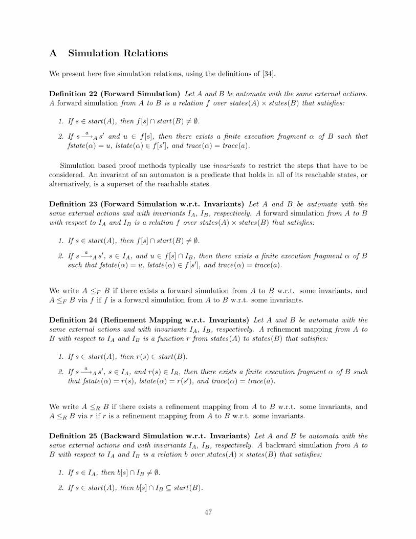
A Simulation Relations

We present here five simulation relations, using the definitions of [34].

Definition 22 (Forward Simulation) Let A and B be automata with the same external actions.A forward simulation from A to B is a relation f over states(A) × states(B) that satisfies:

1. If s ∈ start(A), then f [s] ∩ start(B) 6= ∅.

2. If sa

−→A s′ and u ∈ f [s], then there exists a finite execution fragment α of B such that

fstate(α) = u, lstate(α) ∈ f [s′], and trace(α) = trace(a).

Simulation based proof methods typically use invariants to restrict the steps that have to beconsidered. An invariant of an automaton is a predicate that holds in all of its reachable states, oralternatively, is a superset of the reachable states.

Definition 23 (Forward Simulation w.r.t. Invariants) Let A and B be automata with thesame external actions and with invariants IA, IB, respectively. A forward simulation from A to Bwith respect to IA and IB is a relation f over states(A) × states(B) that satisfies:

1. If s ∈ start(A), then f [s] ∩ start(B) 6= ∅.

2. If sa

−→A s′, s ∈ IA, and u ∈ f [s] ∩ IB, then there exists a finite execution fragment α of B

such that fstate(α) = u, lstate(α) ∈ f [s′], and trace(α) = trace(a).

We write A ≤F B if there exists a forward simulation from A to B w.r.t. some invariants, andA ≤F B via f if f is a forward simulation from A to B w.r.t. some invariants.

Definition 24 (Refinement Mapping w.r.t. Invariants) Let A and B be automata with thesame external actions and with invariants IA, IB, respectively. A refinement mapping from A toB with respect to IA and IB is a function r from states(A) to states(B) that satisfies:

1. If s ∈ start(A), then r(s) ∈ start(B).

2. If sa

−→A s′, s ∈ IA, and r(s) ∈ IB, then there exists a finite execution fragment α of B such

that fstate(α) = r(s), lstate(α) = r(s′), and trace(α) = trace(a).

We write A ≤R B if there exists a refinement mapping from A to B w.r.t. some invariants, andA ≤R B via r if r is a refinement mapping from A to B w.r.t. some invariants.

Definition 25 (Backward Simulation w.r.t. Invariants) Let A and B be automata with thesame external actions and with invariants IA, IB, respectively. A backward simulation from A toB with respect to IA and IB is a relation b over states(A) × states(B) that satisfies:

1. If s ∈ IA, then b[s] ∩ IB 6= ∅.

2. If s ∈ start(A), then b[s] ∩ IB ⊆ start(B).

47

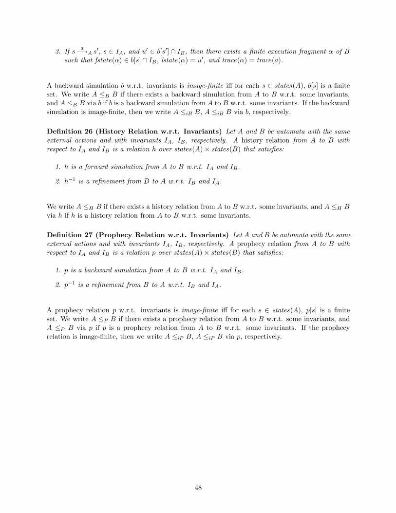
3. If sa

−→A s′, s ∈ IA, and u′ ∈ b[s′] ∩ IB, then there exists a finite execution fragment α of B

such that fstate(α) ∈ b[s] ∩ IB, lstate(α) = u′, and trace(α) = trace(a).

A backward simulation b w.r.t. invariants is image-finite iff for each s ∈ states(A), b[s] is a finiteset. We write A ≤B B if there exists a backward simulation from A to B w.r.t. some invariants,and A ≤B B via b if b is a backward simulation from A to B w.r.t. some invariants. If the backwardsimulation is image-finite, then we write A ≤iB B, A ≤iB B via b, respectively.

Definition 26 (History Relation w.r.t. Invariants) Let A and B be automata with the sameexternal actions and with invariants IA, IB, respectively. A history relation from A to B withrespect to IA and IB is a relation h over states(A) × states(B) that satisfies:

1. h is a forward simulation from A to B w.r.t. IA and IB.

2. h−1 is a refinement from B to A w.r.t. IB and IA.

We write A ≤H B if there exists a history relation from A to B w.r.t. some invariants, and A ≤H Bvia h if h is a history relation from A to B w.r.t. some invariants.

Definition 27 (Prophecy Relation w.r.t. Invariants) Let A and B be automata with the sameexternal actions and with invariants IA, IB, respectively. A prophecy relation from A to B withrespect to IA and IB is a relation p over states(A) × states(B) that satisfies:

1. p is a backward simulation from A to B w.r.t. IA and IB.

2. p−1 is a refinement from B to A w.r.t. IB and IA.

A prophecy relation p w.r.t. invariants is image-finite iff for each s ∈ states(A), p[s] is a finiteset. We write A ≤P B if there exists a prophecy relation from A to B w.r.t. some invariants, andA ≤P B via p if p is a prophecy relation from A to B w.r.t. some invariants. If the prophecyrelation is image-finite, then we write A ≤iP B, A ≤iP B via p, respectively.

48

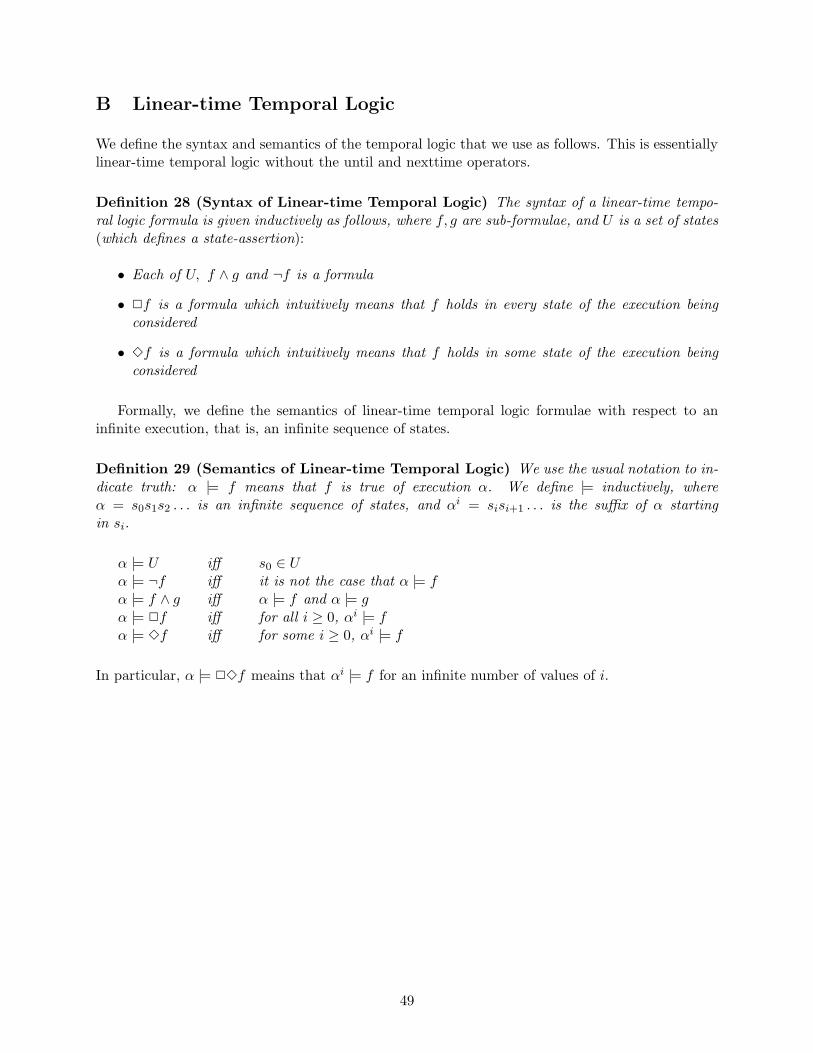
B Linear-time Temporal Logic

We define the syntax and semantics of the temporal logic that we use as follows. This is essentiallylinear-time temporal logic without the until and nexttime operators.

Definition 28 (Syntax of Linear-time Temporal Logic) The syntax of a linear-time tempo-ral logic formula is given inductively as follows, where f, g are sub-formulae, and U is a set of states(which defines a state-assertion):

• Each of U, f ∧ g and ¬f is a formula

• 2f is a formula which intuitively means that f holds in every state of the execution beingconsidered

• 3f is a formula which intuitively means that f holds in some state of the execution beingconsidered

Formally, we define the semantics of linear-time temporal logic formulae with respect to aninfinite execution, that is, an infinite sequence of states.

Definition 29 (Semantics of Linear-time Temporal Logic) We use the usual notation to in-dicate truth: α |= f means that f is true of execution α. We define |= inductively, whereα = s0s1s2 . . . is an infinite sequence of states, and αi = sisi+1 . . . is the suffix of α startingin si.

α |= U iff s0 ∈ Uα |= ¬f iff it is not the case that α |= fα |= f ∧ g iff α |= f and α |= gα |= 2f iff for all i ≥ 0, αi |= fα |= 3f iff for some i ≥ 0, αi |= f

In particular, α |= 23f meains that αi |= f for an infinite number of values of i.

49

C I/O Automaton Code for the ESDS Example, from [14]

I/O Automaton Users

Signature

Input:response(x, v), where x ∈ O and v ∈ V

Output:request(x), where x ∈ O

State

requested , a subset of O, initially empty

Actions

Output request(x)Pre: x.id /∈ requested .id

x.prev ⊆ requested .idEff: requested ← requested ∪ {x}

Input response(x, v)Eff: None

Figure 7: The Users Automaton

50

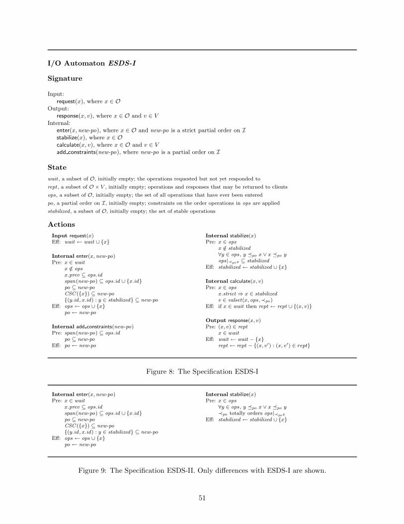
I/O Automaton ESDS-I

Signature

Input:request(x), where x ∈ O

Output:response(x, v), where x ∈ O and v ∈ V

Internal:enter(x,new-po), where x ∈ O and new-po is a strict partial order on I

stabilize(x), where x ∈ O

calculate(x, v), where x ∈ O and v ∈ V

add constraints(new-po), where new-po is a partial order on I

State

wait , a subset of O, initially empty; the operations requested but not yet responded to

rept , a subset of O × V , initially empty; operations and responses that may be returned to clients

ops, a subset of O, initially empty; the set of all operations that have ever been entered

po, a partial order on I, initially empty; constraints on the order operations in ops are applied

stabilized , a subset of O, initially empty; the set of stable operations

Actions

Input request(x)Eff: wait ← wait ∪ {x}

Internal enter(x, new-po)Pre: x ∈ wait

x /∈ ops

x.prev ⊆ ops.idspan(new-po) ⊆ ops.id ∪ {x.id}po ⊆ new-po

CSC ({x}) ⊆ new-po

{(y.id , x.id) : y ∈ stabilized} ⊆ new-po

Eff: ops ← ops ∪ {x}po ← new-po

Internal add constraints(new-po)Pre: span(new-po) ⊆ ops.id

po ⊆ new-po

Eff: po ← new-po

Internal stabilize(x)Pre: x ∈ ops

x /∈ stabilized

∀y ∈ ops , y �po x ∨ x �po yops|≺pox ⊆ stabilized

Eff: stabilized ← stabilized ∪ {x}

Internal calculate(x, v)Pre: x ∈ ops

x.strict ⇒ x ∈ stabilized

v ∈ valset(x, ops ,≺po)Eff: if x ∈ wait then rept ← rept ∪ {(x, v)}

Output response(x, v)Pre: (x, v) ∈ rept

x ∈ waitEff: wait ← wait − {x}

rept ← rept − {(x, v′) : (x, v′) ∈ rept}

Figure 8: The Specification ESDS-I

Internal enter(x, new-po)Pre: x ∈ wait

x.prev ⊆ ops.idspan(new-po) ⊆ ops.id ∪ {x.id}po ⊆ new-po

CSC ({x}) ⊆ new-po

{(y.id , x.id) : y ∈ stabilized} ⊆ new-po

Eff: ops ← ops ∪ {x}po ← new-po

Internal stabilize(x)Pre: x ∈ ops

∀y ∈ ops , y �po x ∨ x �po y≺po totally orders ops|≺pox

Eff: stabilized ← stabilized ∪ {x}

Figure 9: The Specification ESDS-II. Only differences with ESDS-I are shown.

51

I/O Automaton Frontend (c)

Signature

Input:request(x), where x ∈ O and c = client(x)receiverc(m), where r is a replica and m ∈ Mresp

Output:response(x, v), where x ∈ O, c = client(x), and v ∈ V

sendcr(m), where r is a replica and m ∈ Mreq

State

waitc, a subset of O, initially empty

reptc, a subset of O × V , initially empty

Actions

Input request(x)Eff: waitc ← waitc ∪ {x}

Output sendcr(〈“request”, x〉)Pre: x ∈ waitc

Eff: None

Input receiverc(〈“response”, x, v〉)Eff: if x ∈ waitc then reptc ← reptc ∪ {(x, v)}

Output response(x, v)Pre: (x, v) ∈ reptc

x ∈ waitc

Eff: waitc ← waitc − {x}reptc ← reptc − {(x, v′) : (x, v′) ∈ reptc}

Figure 10: The Automaton for the front end of client c

52

I/O Automaton Replica(r)

Signature

Input:receivecr(m), where c is a client and m ∈ Mreq

receiver′r(m), where r′ 6= r is a replica and m ∈ Mgossip

Output:sendrc(m), where c is a client and m ∈ Mresp

sendrr′(m), where r′ 6= r is a replica and m ∈ Mgossip

Internal:do itr(x, l), where x ∈ O and l ∈ Lr

State

pendingr, a subset of O, initially empty; the messages that require a response

rcvdr , a subset of O, initially empty; the operations that have been received

doner[i] for each replica i, a subset of O, initially empty; the operations r knows are done at i

stabler [i] for each replica i, a subset of O, initially empty; the operations r knows are stable at i

labelr : I → L ∪ {∞}, initially all ∞; the minimum label r has seen for id ∈ I

Derived variable: lcr = {(id , id ′) : labelr(id) < labelr(id ′)}, a strict partial order on I; the local constraints at r

Actions

Input receivecr(〈“request”, x〉)Eff: pendingr ← pendingr ∪ {x}

rcvdr ← rcvdr ∪ {x}

Internal do itr(x, l)Pre: x ∈ rcvdr − doner[r]

x.prev ⊆ doner[r].idl > labelr(y.id) for all y ∈ doner [r]

Eff: doner[r]← doner [r] ∪ {x}labelr(x.id)← l

Output sendrc(〈“response”, x, v〉)Pre: x ∈ pendingr ∩ doner [r]

x.strict ⇒ x ∈T

i stabler[i]v ∈ valset(x, doner[r],≺lcr

)c = client(x)

Eff: pendingr ← pendingr − {x}

Output sendrr′(〈“gossip”, R, D, L, S〉)Pre: R = rcvdr ; D = doner[r];

L = labelr ; S = stabler[r]

Input receiver′r(〈“gossip”, R, D, L, S〉)Eff: rcvdr ← rcvdr ∪ R

doner [r′]← doner [r′] ∪D ∪ Sdoner [r]← doner[r] ∪D ∪ Sdoner [i]← doner[i] ∪ S for all i 6= r, r′

labelr ← min(labelr, L)stabler[r′]← stabler[r′] ∪ Sstabler[r]← stabler [r] ∪ S ∪ (

T

i doner [i])

Figure 11: Automaton for replica r

53

I/O Automaton Channel (i, j,M)

Signature

Input:sendij(m), where m ∈ M

Output:receiveij(m), where m ∈ M

State

channel ij , a multiset of messages, (taken fromM), initially empty

Actions

Input sendij(m)Eff: channel ij ← channel ij ∪ {m}

Output receiveij(m)Pre: m ∈ channel ijEff: channel ij ← channel ij − {m}

Figure 12: The Channel Automaton

54