ON THE RELATION OF INTERACTION SEMANTICS TO … · · 2014-12-16Ludwig-Maximilians-Universit at...
41
Logical Methods in Computer Science Vol. 10(4:10)2014, pp. 1–41 www.lmcs-online.org Submitted Dec. 30, 2013 Published Dec. 16, 2014 ON THE RELATION OF INTERACTION SEMANTICS TO CONTINUATIONS AND DEFUNCTIONALIZATION ULRICH SCH ¨ OPP Ludwig-Maximilians-Universit¨ at M¨ unchen, Germany e-mail address : Ulrich.Schoepp@ifi.lmu.de Abstract. In game semantics and related approaches to programming language semantics, programs are modelled by interaction dialogues. Such models have recently been used in the design of new compilation methods, e.g. for hardware synthesis or for programming with sublinear space. This paper relates such semantically motivated non-standard compilation methods to more standard techniques in the compilation of functional programming languages, namely continuation passing and defunctionalization. We first show for the linear λ-calculus that interpretation in a model of computation by interaction can be described as a call-by-name CPS-translation followed by a defunctionalization procedure that takes into account control-flow information. We then establish a relation between these two compilation methods for the simply-typed λ-calculus and end by considering recursion. 1. Introduction A successful approach in the semantics of programming languages is to model programs using interaction dialogues. It is fundamental to Game Semantics [23, 2], the Geometry of Interaction [17] and related lines of research. The idea goes back to the study of dialogical models of constructive logic [27], which explain the meaning of a logical sentence by how one can attack and defend it in a debate [6]. A proof of a sentence is a strategy for defending it against any possible attack. In programming language semantics, types take the place of sentences and attacks can be seen as requests for information. The meaning of a program is a strategy that explains how to answer any possible request. Programs are interpreted compositionally, so that the answer to a request depends only on how the parts of the programs answer to suitable requests. Computation is thus modelled as an interaction dialogue. While interaction dialogues are typically considered as abstract mathematical objects, it has also been argued that they are useful for implementing actual computation. To compute the result of a program it is enough to have an implementation of the strategy that interprets it, i.e. a implementation that takes requests as input and that computes the strategies’ answer as output. The compositional definition of the interactive interpretation guides the 2012 ACM CCS: [Theory of computation]: Semantics and reasoning—Program semantics. Key words and phrases: CPS-translation, Defunctionalization, Int-construction, Game Semantics, Geome- try of Interaction. LOGICAL METHODS IN COMPUTER SCIENCE DOI:10.2168/LMCS-10(4:10)2014 c U. Schöpp CC Creative Commons
Transcript of ON THE RELATION OF INTERACTION SEMANTICS TO … · · 2014-12-16Ludwig-Maximilians-Universit at...
Logical Methods in Computer ScienceVol. 10(4:10)2014, pp. 1–41www.lmcs-online.org
Submitted Dec. 30, 2013Published Dec. 16, 2014
ON THE RELATION OF INTERACTION SEMANTICS TO
CONTINUATIONS AND DEFUNCTIONALIZATION
ULRICH SCHOPP
Ludwig-Maximilians-Universitat Munchen, Germanye-mail address: [email protected]
Abstract. In game semantics and related approaches to programming language semantics,programs are modelled by interaction dialogues. Such models have recently been used in thedesign of new compilation methods, e.g. for hardware synthesis or for programming withsublinear space. This paper relates such semantically motivated non-standard compilationmethods to more standard techniques in the compilation of functional programminglanguages, namely continuation passing and defunctionalization. We first show for thelinear λ-calculus that interpretation in a model of computation by interaction can bedescribed as a call-by-name CPS-translation followed by a defunctionalization procedurethat takes into account control-flow information. We then establish a relation betweenthese two compilation methods for the simply-typed λ-calculus and end by consideringrecursion.
1. Introduction
A successful approach in the semantics of programming languages is to model programsusing interaction dialogues. It is fundamental to Game Semantics [23, 2], the Geometry ofInteraction [17] and related lines of research. The idea goes back to the study of dialogicalmodels of constructive logic [27], which explain the meaning of a logical sentence by how onecan attack and defend it in a debate [6]. A proof of a sentence is a strategy for defending itagainst any possible attack. In programming language semantics, types take the place ofsentences and attacks can be seen as requests for information. The meaning of a programis a strategy that explains how to answer any possible request. Programs are interpretedcompositionally, so that the answer to a request depends only on how the parts of theprograms answer to suitable requests. Computation is thus modelled as an interactiondialogue.
While interaction dialogues are typically considered as abstract mathematical objects, ithas also been argued that they are useful for implementing actual computation. To computethe result of a program it is enough to have an implementation of the strategy that interpretsit, i.e. a implementation that takes requests as input and that computes the strategies’answer as output. The compositional definition of the interactive interpretation guides the
2012 ACM CCS: [Theory of computation]: Semantics and reasoning—Program semantics.Key words and phrases: CPS-translation, Defunctionalization, Int-construction, Game Semantics, Geome-
try of Interaction.
LOGICAL METHODSl IN COMPUTER SCIENCE DOI:10.2168/LMCS-10(4:10)2014c© U. SchöppCC© Creative Commons

2 U. SCHOPP
construction of such an implementation. For example, one may implement the strategyfor each program part by a separate module. The compositional translation of programsexplain how to assemble such modules to obtain the implementation of a whole program.The modules interact with each other by a suitable form of message passing and implementthe computation by playing out actual interaction dialogues. Implementations of this kindhave been proposed for example in [12, 13, 8].
One main motivation for studying the implementation of interaction models is to guidethe design of compilation methods for programming languages. Interaction models aretypically quite concrete and suitable for implementation in simple low-level languages, but,at the same time, they have rich structure and provide accurate models for sophisticatedprogramming languages, see e.g. [2, 23, 32].
The approach of using interactive semantics as an implementation technique for program-ming languages has been proposed in a variety of contexts. Mackie [28] uses ideas from theGeometry of Interaction for the implementation of functional languages. In later work it wasnoticed that such ideas are useful especially for the implementation of functional languageswith strong resource constraints. Ghica et al. have developed methods for hardware synthesisbased on Game Semantics [14, 16]. A related semantic approach has been used to designa functional programming language for sublinear space computation [8]. Other work hasbeen motivated by the idea that strategies are implemented by communicating modules.This has inspired work on fully abstract translations from PCF to the π-calculus, suchas [22, 5]. It has also been used to apply ideas from Game Semantics and the Geometry ofInteraction for distributed computing [12]. In another direction, the Geometry of Interactionis being used as a basis for structuring quantum computation [20, 42]. This list of examplesis certainly not exhaustive; it illustrates the wide range of applications of the implementationof interactive dialogues.
The aim of this paper is to relate compilation methods based on interaction semanticsto standard techniques in the efficient compilation of functional programming languages. Ithas been observed before, for example by Mellies [29] and Levy [26], that interaction modelsare related to continuation passing, an important standard technique in the compilationof functional programming languages [3]. In this paper we make a further connection todefunctionalization [36].
We consider the compilation of higher-order languages, such as PCF. A compiler wouldtransform such a language to machine code by way of a number of intermediate languages.Typically, the higher-order source code would first be translated to first-order intermediatecode, from which the machine code is then generated. This paper is concerned with the firststep, the translation from higher-order to first-order code. We show that the composition oftwo well-known transformations, namely CPS-translation [35] and defunctionalization [36],is closely related to an interpretation of the source language in a model that implementsinteraction dialogues.
The interactive model we study in this paper is an instance of the Int construction [25].This model is very basic and captures only what is needed for its intended application asan implementation technique. We believe that it is a good choice, as the Int constructionhas been identified as the core of a number of interactive semantics, so that our resultsapply to a number of interactive models. Indeed, in [1] it was shown that the (particle style)Geometry of Interaction can be seen as an instance of the Int construction with furtherstructure. Abramsky-Jagadeesan-Malacaria (AJM) games [2] are also closely related to theInt construction. AJM games refine the Int construction by removing unwanted interaction

INTERACTION SEMANTICS, CONTINUATIONS AND DEFUNCTIONALIZATION 3
dialogues and by integrating a quotient to capture a good notion of program equality, seethe construction in [2]. If one is interested only in implementing strategies, then one mayrestrict ones attention to the core given only by the Int construction.
In order to define an interpretation of a higher-order source language in an interactivemodel given by the Int construction, we build on work reported in [8]. As the resultinginterpretation implements call-by-name, we relate it to a call-by-name CPS-translation – avariant of the one by Hofmann and Streicher [21].
Let us outline concretely how CPS-translation, defunctionalization and the interpretationin an interactive model are related by looking at the very simple example of a function thatincrements a natural number: λx:N. 1 + x. We next outline how this function is translatedby the two approaches and how the results compare.
1.1. CPS-Translation and Defunctionalization. A compiler for PCF might first trans-form λx:N. 1 + x into continuation passing style, perhaps apply some optimisations, and thenuse defunctionalization to obtain a first-order intermediate program, ready for compilationto machine language.
Hofmann and Streicher’s call-by-name CPS-translation [21] translates the source termλx:N. 1 + x to λ〈x, k〉. (λk.k 1) (λu. x (λn. k (u+n))) : ¬(¬¬N׬N), where we write ¬A forA→ ⊥. This term defines a function, which takes as argument a pair 〈x, k〉 of a continuationk : ¬N that accepts the result and a variable x : ¬¬N that supplies the function argument.To obtain the actual function argument, one applies x to a continuation (here λn. k (u+ n))to ask for the actual argument to be thrown into the supplied continuation.
Defunctionalization [36] translates this higher-order term into a first-order program.The basic idea is to give each function a name and to pass around not the function itself,but only its name and the values of its free variables. To this end, each λ-abstraction isnamed with a unique label: λl1〈x, k〉. (λl2k.k 1) (λl3u. x (λl4n. k (u+ n))). The whole termdefines the function named with label l1. It can be represented simply by the label l1. Thefunction with label l3 has free variables x and k and is represented by the label togetherwith the values of x and k, which we write as l3(x, k).
Each application s t is replaced by a procedure call apply(s, t), as s is now only the nameof a function and not a function itself. The procedure apply is defined by case distinction onthe function name and behaves like the body of the respective λ-abstraction in the originalterm. In the example, we have the following definition of apply:
apply(f, a) = case f of l1 ⇒ let 〈x, k〉 = a in apply(l2, l3(x, k))
| l2 ⇒ apply(a, 1)
| l3(x, k)⇒ apply(x, l4(k, a))
| l4(k, u)⇒ apply(k, u+ a)
This definition should be understood as the recursive definition of a function apply with twoarguments. The definition is untyped, as in Reynold’s original definition of defunctionaliza-tion [36].
To understand concretely how this definition represents the original term, it is perhapsuseful to see what happens when a concrete argument and a continuation are supplied:(λl1〈x, k〉. (λl2k.k 1) (λl3u. x (λl4n. k (u+n)))) 〈λl5k. k 42, λl6n. print int(n)〉. The definition

4 U. SCHOPP
of apply then has two cases for l5 and l6 in addition to the cases above:
apply(l, a) = case l of . . .
| l5 ⇒ apply(a, 42)
| l6 ⇒ print int(n)
The fully applied term defunctionalizes to apply(l1, 〈l5, l6〉). Executing it results in 43 beingprinted. When we evaluate apply(l1, 〈l5, l6〉), the first case in the definition of apply appliesand results in the call apply(l2, l3(l5, l6)). For this call, the second case applies, so thatthe call apply(l3(l5, l6), 1) is made. The computation continues in this way with calls toapply(l5, l4(l6, 1)), apply(l4(l6, 1), 42), apply(l6, 43), and finally print int(43).
This outlines a naive defunctionalization method for translating a higher-order languageinto a first-order language with (tail) recursion. This method can be improved in variousways. The above apply-function performs a case distinction on the function name each timeit is invoked. However, in the example it is possible to determine the label in the firstargument of each appearance of apply statically, so that the case distinction is not necessary.Instead, we may define one function applyl for each label l and replace apply(l(x), a) byapplyl(x, a). The label l thus does not need to be passed as an argument anymore. Adefunctionalization procedure that takes into account control flow information in this waywas introduced by Banerjee et al. [4]. If we apply it to this example and moreover simplifythe result by removing unneeded function arguments, then we get four mutually recursivefunctions:
applyl1() = applyl2() applyl2() = applyl3(1)
applyl3(u) = applyl5(u) applyl4(u, n) = applyl6(u+ n)(1.1)
The term itself simplifies to applyl1(). The interface where these equations interact withthe environment consists of the labels l1 (the entry label), l6 (the return label), l5 (theentry label for argument function x) and l4 (the return label for the argument function x).Applying the term to concrete arguments as above amounts to extending the environmentwith the following equations:
applyl5(u) = applyl4(u, 42) applyl6(n) = print int(n)
The point of this paper is that the program (1.1) is just what we get from interpretingthe source term in a model of computation by interaction.
1.2. Interpretation in an Interactive Computation Model. In computation by in-teraction the general idea is to study models of computation that interpret programs byinteraction dialogues and to consider actual implementations of such dialogue interaction.For example, a function of type N→ N may be implemented in interactive style by a programthat, for a suitable type S, takes as input a value of type unit + (S × nat) and gives asoutput a value of type nat + (S × unit). The input inl(〈〉) to this program is interpreted asa request for the return value of the function. An output of the form inl(n) means that n isthe requested value. If the output is of the form inr(s, 〈〉), however, then this means thatthe program would like to know the argument of the function. It also requests that thevalue s be returned along with the answer. Programs here do not have state and have nopersistent memory to store any data until a request is answered. The program can howeverencode any data that it needs later in the value s and ask for this value to be returnedunchanged with the answer to its request. For the outside, the value s is opaque. We do not

INTERACTION SEMANTICS, CONTINUATIONS AND DEFUNCTIONALIZATION 5
know anything about what is encoded in the value s, only that we have to give it back withthe answer to the request. To answer the program’s request, we pass a value of the forminr(s,m), where m is our answer.
The particular function λx:N. 1 + x is implemented by the program specified in thefollowing diagram, where S is nat. This diagram is to be understood so that one may pass amessage along any of its input wires. The message must be a value of the type labelling thewire. When a message arrives at an input of box, the box will react by sending a messageon one of its outputs. Thus, at any time there is one message in the network. Computationends when a message is passed along an output wire.
l3
add
one
nat
nat nat× unitnat× nat unit
unit l1l4
l2
l6l5
In this diagram, add has three input ports of type unit, nat × nat and nat respectivelyfrom top to bottom. It may output a message on one of its three output ports, which havetype nat, nat× unit and unit from top to bottom. Its behaviour is given as follows: if itreceives message 〈〉 on the topmost input port (a request for the sum), then it outputs 〈〉 onthe bottom output port (a request to provide the first summand); if it receives n on thebottom input port (the first summand), then it outputs 〈n, 〈〉〉 on the middle output port(a request to provide the second summand and to hold on to the first summand until therequest is answered); and if it receives 〈n,m〉 on the middle input port (both summands), itoutputs n+m on the topmost output port. The box labelled one maps the request 〈〉 tothe number 1.
This interactive implementation of λx:N. 1 + x may be described as the interpretation ofthe term in a semantic model Int(T) built by applying the general categorical Int constructionto a category T that is constructed from the target language, see Section 6.
Compare the above interaction diagram to the definitions in (1.1) obtained by defunc-tionalization. The labels l1, l4 and l3 there correspond to the three input ports of theadd-box (from top to bottom), l2 is the input of box one, and l5 and l6 are the destinationlabels of the two outgoing wires. One may consider the apply-definitions in (1.1) a particularimplementation of the diagram, where a call to applyl(m) means that message m is sent topoint l in the diagram. A naive implementation would introduce a label for the end of eacharrow in the diagram and implement the message passing accordingly.
1.3. Overview. The subject of this paper is the relation of the two translations that wehave just outlined. The paper studies the following situation of two translations from asource language that is a variant of PCF into a simple first-order target language with tailrecursion.
source
target
Int interpretation CPS-translation;defunctionalization

6 U. SCHOPP
After giving definitions of the source and target language in the following two sections,we find it useful to present and analyse the above situation step by step. We define the twotranslations and study their relationship for a number of fragments of the source languageof increasing strength.
core ⊆ lin ⊆ stl ⊆ source
In Section 6 we start by studying the translation for the source fragment core. Thisfragment contains just a bare minimum of linear λ-abstraction and application. It isnevertheless instructive to consider this fragment as a setting in which to develop theinfrastructure for the translation of higher-order functions.
In Section 7 we consider the fragment lin, which extends core with a base type ofnatural numbers. Rather than studying the above situation directly with lin in place ofsource, we argue that it is useful to take a detour over a calculus linexp, which is a versionof lin with additional type annotations. These type annotations are useful for understandingthe Int-interpretation.
In Section 8 we then add contraction and come to the simply typed fragment stl of thesource language. We first continue to use additional type annotations and extend linexp tostlexp. We then come back to the unannotated source fragment stl by showing how stlcan be translated into stlexp (Prop. 8.7).
In Section 9 we finally then extend the translation to the full source language by addingrecursion.
2. Target Language
Programs in the target language consist of mutually tail-recursive definitions of first-orderfunctions, such as the apply-equations above. One should think of the target language asa simple variant of SSA-form compiler intermediate languages, e.g. [7], in which functiondefinitions are often presented as labelled blocks that end with a jump to a label.
The target language does not model function calls or a calling convention; it modelsonly what one would use for the compilation of a single unit. Certain function labels aredesignated as entry or exit points. In the following example target program the labels constand pow are intended as entry points.
const(x) = const ret(23)
pow(〈x, y〉) = pow loop(〈x, y〉)pow loop(〈x, y〉) = case iszero(x) of inl(z)⇒ pow ret(y)
; inr(z)⇒ pow loop(〈x− 1, y ∗ y〉)The function labels const ret and pow ret are exit points that are assumed to be definedexternally and that are used to return the results of computations.
A target program will be a set of equations together with lists of entry and exit labelsthat specify the interface of the program. Target programs are defined in detail in the restof this section. Upon first reading, the reader may wish to skim this section only.
Target programs are typed. The set of target types is defined by the grammar below.Recursive types will be needed at the end of Section 8 only. Target expressions are standard

INTERACTION SEMANTICS, CONTINUATIONS AND DEFUNCTIONALIZATION 7
terms for these types, see e.g. [34]:
Types: A,B ::= α∣∣ unit
∣∣ nat∣∣ A×B ∣∣ A+B
∣∣ µα.AExpressions: e, e1, e2 ::= x
∣∣ 〈〉 ∣∣ n ∣∣ e1 + e2∣∣ iszero(e)∣∣ 〈e1, e2〉 ∣∣ let 〈x, y〉 = e1 in e2∣∣ inl(e)
∣∣ inr(e)∣∣ case e of inl(x)⇒ e1; inr(y)⇒ e2∣∣ foldA(e)
∣∣ unfoldA(e)
In the syntax, α ranges over type variables, x over expression variables, and n over naturalnumbers as constants. We identify terms up to renaming of bound variables. The termlet 〈x, y〉 = e1 in e2 binds the variables x and y in e2 and case e of inl(x)⇒ e1; inr(y)⇒ e2binds variable x in e1 and variable y in e2. The term iszero(e) is intended to have typeunit + unit, with inl(〈〉) representing true.
We remark that the type nat is used solely to encode values of the source type of naturalnumbers N. For applications to compilation, one may be interested in restricting the naturalnumbers to, say, 64-bit integers. Such a restriction can be made without affecting the resultsin this paper.
Target expressions are typed with a standard type system, see Figure 1. A judgementΓ ` e : A therein expresses that e has type A in context Γ, where Γ is a finite mapping fromvariables to target types.
For convenience, we allow ourselves ML-like data type notation for working with recursivetypes. For example, for a type of lists we may write
β list = datatype nil of unit | cons of β × (β list)
instead of µα. unit + β × α, as cons(x, l) is more readable than foldµα. unit+β×α(inr(〈x, l〉)).For the operational semantics of target expressions we define a standard call-by-value
small-step reduction relation. We use the concepts of target values and evaluation contexts:
Values: v, w ::= 〈〉∣∣ n ∣∣ 〈v, w〉 ∣∣ inl(v)
∣∣ inr(v)∣∣ foldA(v)
Evaluation Contexts: C ::= []∣∣ C + e
∣∣ v + C∣∣ iszero(C)∣∣ 〈C, e〉 ∣∣ 〈v, C〉 ∣∣ let 〈x, y〉 = C in e∣∣ inl(C)
∣∣ inr(C)∣∣ case C of inl(x)⇒ e1; inr(y)⇒ e2
The small-step reduction relation is then defined to be the smallest relation −→ satisfyingthe following clauses:
n1 + n2 −→ n3 if n3 is the sum of n1 and n2
iszero(0) −→ inl(〈〉)iszero(n) −→ inr(〈〉) if n is non-zero
let 〈x, y〉 = 〈v1, v2〉 in e −→ e[v1/x, v2/y]
case inl(v) of inl(x)⇒ e1; inr(y)⇒ e2 −→ e1[v/x]
case inr(v) of inl(x)⇒ e1; inr(y)⇒ e2 −→ e2[v/x]
unfold(fold(v)) −→ v
C[e1] −→ C[e2] if e1 −→ e2
Proposition 2.1. For each ` e : A there exists a unique value v satisfying e −→∗ v.
8 U. SCHOPP
x : A in ΓΓ ` x : A Γ ` 〈〉 : unit
Γ ` n : natΓ ` e1 : nat Γ ` e2 : nat
Γ ` e1 + e2 : natΓ ` e : nat
Γ ` iszero(e) : unit + unit
Γ ` e1 : A Γ ` e2 : B
Γ ` 〈e1, e2〉 : A×BΓ ` e1 : A×B Γ, x : A, y : B ` e2 : C
Γ ` let 〈x, y〉 = e1 in e2 : C
Γ ` e : AΓ ` inl(e) : A+B
Γ ` e : BΓ ` inr(e) : A+B
Γ ` e : A+B Γ, x : A ` e1 : C Γ, y : B ` e2 : C
Γ ` case e of inl(x)⇒ e1; inr(y)⇒ e2 : C
Γ ` e : A[µα.A/α]
Γ ` foldµα.A(e) : µα.A
Γ ` e : µα.A
Γ ` unfoldµα.A(e) : A[µα.A/α]
Figure 1: Typing of Target Expressions
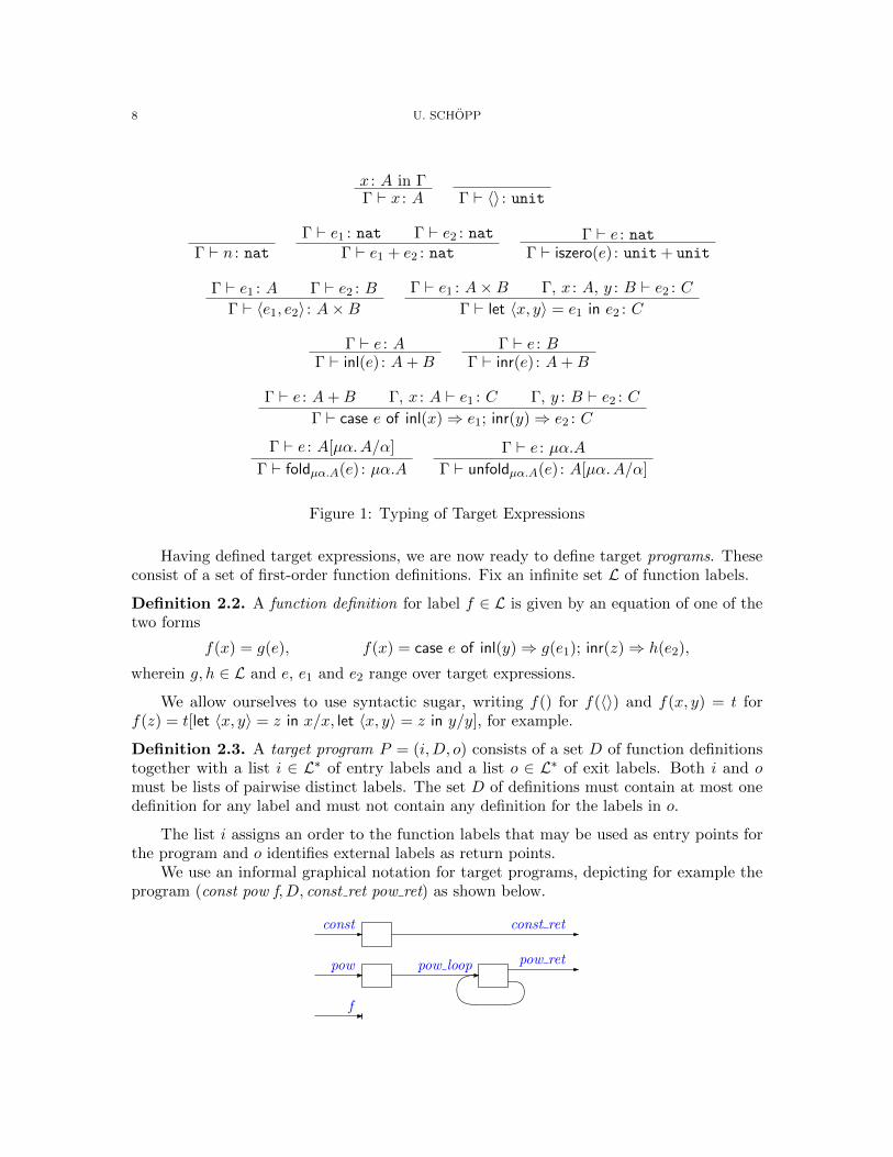
Having defined target expressions, we are now ready to define target programs. Theseconsist of a set of first-order function definitions. Fix an infinite set L of function labels.
Definition 2.2. A function definition for label f ∈ L is given by an equation of one of thetwo forms
f(x) = g(e), f(x) = case e of inl(y)⇒ g(e1); inr(z)⇒ h(e2),
wherein g, h ∈ L and e, e1 and e2 range over target expressions.
We allow ourselves to use syntactic sugar, writing f() for f(〈〉) and f(x, y) = t forf(z) = t[let 〈x, y〉 = z in x/x, let 〈x, y〉 = z in y/y], for example.
Definition 2.3. A target program P = (i,D, o) consists of a set D of function definitionstogether with a list i ∈ L∗ of entry labels and a list o ∈ L∗ of exit labels. Both i and omust be lists of pairwise distinct labels. The set D of definitions must contain at most onedefinition for any label and must not contain any definition for the labels in o.
The list i assigns an order to the function labels that may be used as entry points forthe program and o identifies external labels as return points.
We use an informal graphical notation for target programs, depicting for example theprogram (const pow f, D, const ret pow ret) as shown below.
const
pow pow loop
const ret
pow ret
f
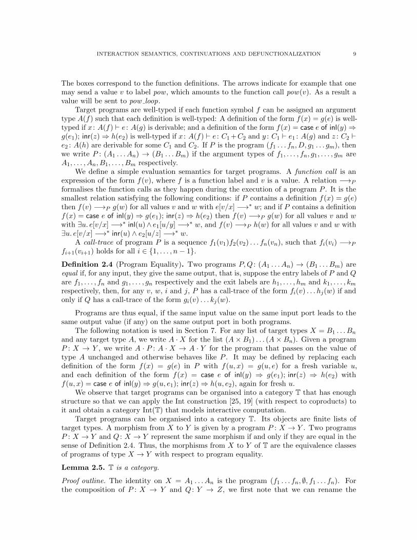
INTERACTION SEMANTICS, CONTINUATIONS AND DEFUNCTIONALIZATION 9
The boxes correspond to the function definitions. The arrows indicate for example that onemay send a value v to label pow , which amounts to the function call pow(v). As a result avalue will be sent to pow loop.
Target programs are well-typed if each function symbol f can be assigned an argumenttype A(f) such that each definition is well-typed: A definition of the form f(x) = g(e) is well-typed if x : A(f) ` e : A(g) is derivable; and a definition of the form f(x) = case e of inl(y)⇒g(e1); inr(z)⇒ h(e2) is well-typed if x : A(f) ` e : C1 +C2 and y : C1 ` e1 : A(g) and z : C2 `e2 : A(h) are derivable for some C1 and C2. If P is the program (f1 . . . fn, D, g1 . . . gm), thenwe write P : (A1 . . . An) → (B1 . . . Bm) if the argument types of f1, . . . , fn, g1, . . . , gm areA1, . . . , An, B1, . . . , Bm respectively.
We define a simple evaluation semantics for target programs. A function call is anexpression of the form f(v), where f is a function label and v is a value. A relation −→P
formalises the function calls as they happen during the execution of a program P . It is thesmallest relation satisfying the following conditions: if P contains a definition f(x) = g(e)then f(v) −→P g(w) for all values v and w with e[v/x] −→∗ w; and if P contains a definitionf(x) = case e of inl(y)⇒ g(e1); inr(z)⇒ h(e2) then f(v) −→P g(w) for all values v and wwith ∃u. e[v/x] −→∗ inl(u)∧ e1[u/y] −→∗ w, and f(v) −→P h(w) for all values v and w with∃u. e[v/x] −→∗ inr(u) ∧ e2[u/z] −→∗ w.
A call-trace of program P is a sequence f1(v1)f2(v2) . . . fn(vn), such that fi(vi) −→P
fi+1(vi+1) holds for all i ∈ {1, . . . , n− 1}.Definition 2.4 (Program Equality). Two programs P,Q : (A1 . . . An) → (B1 . . . Bm) areequal if, for any input, they give the same output, that is, suppose the entry labels of P and Qare f1, . . . , fn and g1, . . . , gn respectively and the exit labels are h1, . . . , hm and k1, . . . , kmrespectively, then, for any v, w, i and j, P has a call-trace of the form fi(v) . . . hj(w) if andonly if Q has a call-trace of the form gi(v) . . . kj(w).
Programs are thus equal, if the same input value on the same input port leads to thesame output value (if any) on the same output port in both programs.
The following notation is used in Section 7. For any list of target types X = B1 . . . Bnand any target type A, we write A ·X for the list (A×B1) . . . (A×Bn). Given a programP : X → Y , we write A · P : A · X → A · Y for the program that passes on the value oftype A unchanged and otherwise behaves like P . It may be defined by replacing eachdefinition of the form f(x) = g(e) in P with f(u, x) = g(u, e) for a fresh variable u,and each definition of the form f(x) = case e of inl(y) ⇒ g(e1); inr(z) ⇒ h(e2) withf(u, x) = case e of inl(y)⇒ g(u, e1); inr(z)⇒ h(u, e2), again for fresh u.
We observe that target programs can be organised into a category T that has enoughstructure so that we can apply the Int construction [25, 19] (with respect to coproducts) toit and obtain a category Int(T) that models interactive computation.
Target programs can be organised into a category T. Its objects are finite lists oftarget types. A morphism from X to Y is given by a program P : X → Y . Two programsP : X → Y and Q : X → Y represent the same morphism if and only if they are equal in thesense of Definition 2.4. Thus, the morphisms from X to Y of T are the equivalence classesof programs of type X → Y with respect to program equality.
Lemma 2.5. T is a category.
Proof outline. The identity on X = A1 . . . An is the program (f1 . . . fn, ∅, f1 . . . fn). Forthe composition of P : X → Y and Q : Y → Z, we first note that we can rename the

10 U. SCHOPP
labels P and Q such that we have P = (i,DP ,m) and Q = (m,DQ, o). The compositionQ ◦ P : X → Z is then given simply by the program (i,DP ∪DQ, o).
Lemma 2.6. The category T has finite coproducts, such that the initial object 0 is givenby the empty list and the object X + Y is given by the concatenation of the lists X and Y .Moreover, T has a uniform trace [19] with respect to these coproducts.
Proof outline. A simple proof can be given by observing that there is a faithful embeddingfrom T to the category of sets and partial functions. The equations that are required toshow then follow from the fact that the category of sets and partial functions has the desiredstructure.
While we would like to emphasise the mathematical structure of target programs givenby the Int construction, in the rest of the paper we shall spell it out concretely rather thanreferring to categorical notions in order to make the paper easier to read.
3. Source Language
Our source language is a variant of PCF, a simply-typed λ-calculus with a basic type N ofnatural numbers and associated constants, as well as a fixed-point combinator for recursion.The intended evaluation strategy is call-by-name.
The source language has the following types and terms.
Types: X,Y ::= 1∣∣ X → Y
∣∣ NTerms: s, t ::= ∗
∣∣ λx:X. t∣∣ s t ∣∣ n ∣∣ s+ t
∣∣ if0 s then t1 else t2∣∣ fixX
We write ¬X as an abbreviation for the type X → ⊥. Again, we identify terms up torenaming of bound variables.
The typing judgement has the form Γ ` t : X, where Γ is a finite list of variabledeclarations x1 : X1, . . . , xn : Xn. We formulate the typing rules so that it is easy to considerfragments of the source language of varying expressiveness. The core rules are those of alinear λ-calculus and are given in Figure 2. The rules for natural numbers appear in Figure 3.We allow an addition operation s+ t instead of the standard successor operation succ(s), asthis gives a simple example to explain the issues with the compilation of multinary operation.Rules for contraction and for the fixed point combinator are given in Figures 4 and 5.
4. CPS-Translation
We use a variant of Hofmann and Streicher’s call-by-name CPS-translation [21], whichtranslates the source language extended with the following rules for product types as well asa type ⊥ without any rules.
Γ ` s : X ∆ ` t : Y×iΓ, ∆ ` 〈s, t〉 : X × Y
Γ ` s : X × Y ∆, x : X, y : Y ` t : Z×eΓ, ∆ ` let 〈x, y〉 = s in t : Z
For each source type X, the type X of its continuations is defined by:
1 = ¬1 N = ¬N X → Y = ¬X × YA continuation for type X → Y is thus a pair of a continuation of type Y , using which theresult can be returned, and a function ¬X to access the argument. A function can request

INTERACTION SEMANTICS, CONTINUATIONS AND DEFUNCTIONALIZATION 11
axx : X ` x : X
1i ` ∗ : 1
Γ ` t : YweakΓ, x : X ` t : Y
Γ, y : Y, x : X, ∆ ` t : Zexch
Γ, x : X, y : Y, ∆ ` t : Z
Γ, x : X ` t : Y→iΓ ` λx:X. t : X → Y
Γ ` s : X → Y ∆ ` t : X→eΓ, ∆ ` s t : Y
Figure 2: Source Language (core) – Linear Core
num ` n : NΓ ` s : N ∆ ` t : Nadd
Γ, ∆ ` s+ t : NΓ ` s : N ∆1 ` t1 : N ∆2 ` t2 : N
ifΓ, ∆1, ∆2 ` if0 s then t1 else t2 : N
Figure 3: Source Language (lin) – Natural Numbers
Γ, y : X, z : X ` t : Ycontr
Γ, x : X ` t[x/y, x/z] : Y
Figure 4: Source Language (stl) – Contraction
fix ` fixX : (X → X)→ X
Figure 5: Source Language – Recursion
its argument by applying this function to a continuation of type X. The argument will thenbe provided to this continuation.
For computation in continuation passing style, we often use the type ¬X, which wedenote by X.
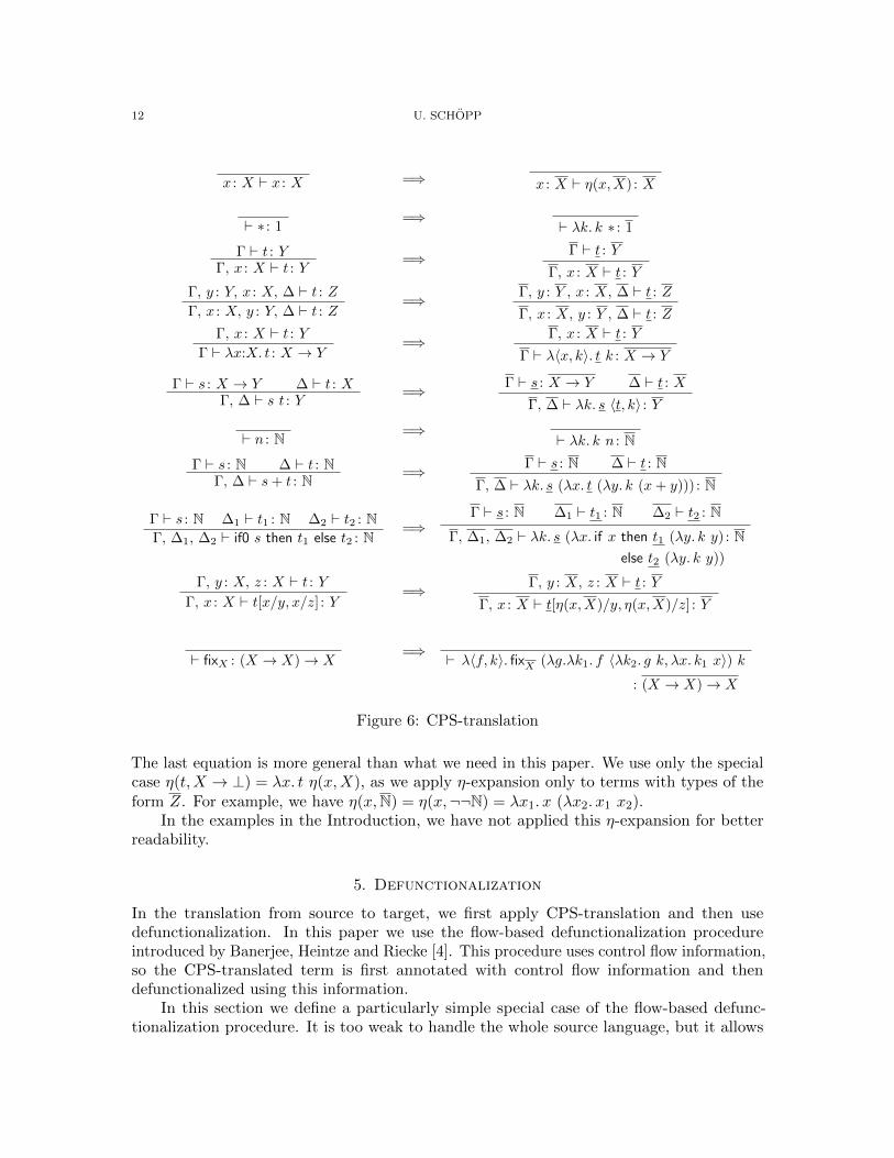
The CPS-translation translates the source language into itself, translating any typingderivation of x1 : X1, . . . , xn : Xn ` t : Y into a derivation of x1 : X1, . . . , xn : Xn ` t : Y . Itis defined by induction on the given typing derivation. Figure 6 shows how each typing ruleon the left is translated to a derived rule on the right.
This CPS-translation differs from the standard call-by-name CPS-translation of [21] inthe use of η-expansion in the rules for variables and contraction. These expansions will allowus to use compositional reasoning in Sections 6-8. The term η(t,X) is defined by inductionon the type X:
η(t,X) = t if X is a base type (1, N or ⊥)
η(t,X × Y ) = let 〈x, y〉 = t in 〈η(x,X), η(y, Y )〉η(t,X → Y ) = λx. η(t η(x,X), Y ) where x is fresh.
12 U. SCHOPP
x : X ` x : X =⇒ x : X ` η(x,X) : X
` ∗ : 1=⇒ ` λk. k ∗ : 1
Γ ` t : YΓ, x : X ` t : Y =⇒ Γ ` t : Y
Γ, x : X ` t : YΓ, y : Y, x : X, ∆ ` t : ZΓ, x : X, y : Y, ∆ ` t : Z =⇒ Γ, y : Y , x : X, ∆ ` t : Z
Γ, x : X, y : Y , ∆ ` t : ZΓ, x : X ` t : Y
Γ ` λx:X. t : X → Y=⇒ Γ, x : X ` t : Y
Γ ` λ〈x, k〉. t k : X → Y
Γ ` s : X → Y ∆ ` t : XΓ, ∆ ` s t : Y =⇒ Γ ` s : X → Y ∆ ` t : X
Γ, ∆ ` λk. s 〈t, k〉 : Y
` n : N =⇒ ` λk. k n : NΓ ` s : N ∆ ` t : N
Γ, ∆ ` s+ t : N =⇒ Γ ` s : N ∆ ` t : NΓ, ∆ ` λk. s (λx. t (λy. k (x+ y))) : N
Γ ` s : N ∆1 ` t1 : N ∆2 ` t2 : NΓ, ∆1, ∆2 ` if0 s then t1 else t2 : N
=⇒Γ ` s : N ∆1 ` t1 : N ∆2 ` t2 : N
Γ, ∆1, ∆2 ` λk. s (λx. if x then t1 (λy. k y) : Nelse t2 (λy. k y))
Γ, y : X, z : X ` t : YΓ, x : X ` t[x/y, x/z] : Y =⇒ Γ, y : X, z : X ` t : Y
Γ, x : X ` t[η(x,X)/y, η(x,X)/z] : Y
` fixX : (X → X)→ X=⇒ ` λ〈f, k〉. fixX (λg.λk1. f 〈λk2. g k, λx. k1 x〉) k
: (X → X)→ X
Figure 6: CPS-translation
The last equation is more general than what we need in this paper. We use only the specialcase η(t,X → ⊥) = λx. t η(x,X), as we apply η-expansion only to terms with types of theform Z. For example, we have η(x,N) = η(x,¬¬N) = λx1. x (λx2. x1 x2).
In the examples in the Introduction, we have not applied this η-expansion for betterreadability.
5. Defunctionalization
In the translation from source to target, we first apply CPS-translation and then usedefunctionalization. In this paper we use the flow-based defunctionalization procedureintroduced by Banerjee, Heintze and Riecke [4]. This procedure uses control flow information,so the CPS-translated term is first annotated with control flow information and thendefunctionalized using this information.
In this section we define a particularly simple special case of the flow-based defunc-tionalization procedure. It is too weak to handle the whole source language, but it allows

INTERACTION SEMANTICS, CONTINUATIONS AND DEFUNCTIONALIZATION 13
for a simple explanation of the relation to the Int construction. We will extend the de-functionalization procedure in Section 8 to cover the CPS-translation of the whole sourcelanguage.
Control flow information is added to the terms in the form of labelling annotations. Inthe simple variant of the defunctionalization procedure that we describe here, each functionabstraction and application is annotated with a single label from L. Thus, the terms λx:X. tand s t are replaced by λlx:X. t and s@l t respectively, where l ranges over L. The function
type X → Y is replaced by Xl−→ Y , again for any l ∈ L. We write ¬lX for X
l−→ ⊥.We require that each abstraction be uniquely identified by its label, that is, we allow
only terms in which no two abstractions have the same label. In the application s@l t thelabel l expresses that the function s applied here is defined by an abstraction with label l.The typing rules for abstraction and application are modified as follows to enforce thatterms are annotated with correct control flow information.
Γ, x : X ` t : YΓ ` λlx:X. t : X
l−→ Y
Γ ` s : Xl−→ Y ∆ ` t : X
Γ, ∆ ` s@l t : Y
Allowing function types and applications to be annotated with a single label onlyis a real restriction. For example, it is not possible to label and type terms such asλx. 〈x (λy. 0), x (λz. 1)〉. The two abstractions λy. 0 and λz. 1 would each have to be givena unique label, say l1 and l2 respectively. But then in the two uses of the variables x, its
types would have to be Xl1−→ Y and X
l2−→ Y respectively. With the above rules, this isnot possible, as l1 and l2 are different labels. In general, one needs to allow types such as
X{l1,l2}−−−−→ Y with more than a single label for more than one possible definition site, as in
e.g. [4]. We come back to this in Section 8, but up until then the variant with a single labelsuffices and simplifies the exposition.
In the rest of this section we explain how terms of the labelled source language (withproduct types) can be defunctionalized into programs in the target language. We defer thequestion of how to annotate the terms obtained by CPS-translation with labels to latersections (Lemmas 6.2 and 8.3).
The defunctionalization of a term t in the labelled source language consists of a target ex-pression t∗, which denotes the defunctionalized term itself, and a set of target equations D(t),which contains the apply-definitions for defunctionalized function application.
x∗ = x
n∗ = n
(if0 s then t else u)∗ = case iszero(s∗) of inl( )⇒ t∗; inr( )⇒ u∗
〈s, t〉∗ = 〈s∗, t∗〉(let 〈x, y〉 = t in s)∗ = let 〈x, y〉 = t∗ in s∗
(s@l t)∗ = applyl(s
∗, t∗)
(λlx:A. t)∗ = 〈x1, . . . , xn〉 where FV(λx:A. t) = {x1, . . . , xn}

14 U. SCHOPP
In the last case for abstraction we assume some fixed global ordering on all variables, sothat the order of the tuple is well-defined.
D(x) = ∅D(n) = ∅
D(if0 s then t else u) = D(s) ∪D(t) ∪D(u)
D(〈s, t〉) = D(s) ∪D(u)
D(let 〈x, y〉 = t in s) = D(t) ∪D(s)
D(s@l t) = D(s) ∪D(t)
D(λlx:A. t) = D(t) ∪ {applyl(〈x1, . . . , xn〉, x) = t∗}In general, the set D(t) need not consist of function definitions in the strict sense ofDefinition 2.2; it may contain nested case distinctions, for example. This technical issuecould easily be solved in general at the expense of making the technical development a littlemore complicated. However, we shall use defunctionalization only for terms t for which D(t)does in fact only consist of function definitions, so we stick with the above simple definitions.
Note that for closed terms of function type the target expression t∗ is just 〈〉. Since allclosed terms t obtained by CPS-translation are of function type, we therefore consider thedefinition set D(t) as the main result of defunctionalization.
Example 5.1. With label annotations the example from the Introduction becomes the termt given by
λl1z. let 〈x, k〉 = z in (λl2k′. k′@l3 1) @l2 (λl3u. x@l5 (λl4n. k@l6 (u+ n))).
Its type is ¬l1(¬l5¬l4N× ¬l6N). The set D(t) consists of the definitions
applyl1(〈〉, 〈x, k〉) = applyl2(〈〉, 〈x, k〉), applyl2(〈〉, k′) = applyl3(k′, 1),
applyl3(〈x, k〉, u) = applyl5(x, 〈k, u〉), applyl4(〈k, u〉, n) = applyl6(k, u+ n).
Compared to the definitions given in (1.1) in the Introduction, it appears that more data isbeing passed around in these apply-equations. However, consider once again the applicationof t to the concrete arguments from the Introduction. Then one gets the additional equations
applyl5(〈〉, k) = applyl4(k, 42), applyl6(〈〉, n) = print int(n),
and the fully applied term defunctionalizes to applyl1(〈〉, 〈〈〉, 〈〉〉). Thus, all the variables inthe apply-equations only ever store the value 〈〉 or tuples thereof, and these arguments mayjust as well be omitted.
An important point to note is that the defunctionalization procedure yields a set ofdefinition equations, but that it does not specify an interface of entry and exit labels. Whenone applies defunctionalization to a whole closed source programs of ground type, as is usuallydone in compilation, choosing an interface is not important. One would typically just choosea single entry label main and a single exit label exit. If one is interested in compositionality,however, then open terms and terms of higher types must be also considered. Then oneneeds to fix an interface that explains how the free variables are accessed and how highertypes are to be used. In the above example term t, a suitable choice of entry and exit labelswould be l1l4 and l5l4 respectively. We shall explain how to define an interface from theimage of the CPS-translation in the next section.

INTERACTION SEMANTICS, CONTINUATIONS AND DEFUNCTIONALIZATION 15
Of course, the defunctionalization procedure described above is quite simple. In actualapplications one would certainly want to apply optimisations, not least to remove unnecessaryfunction arguments. An example of such an optimisation is lightweight defunctionalization ofBanerjee et al. [4]. We shall argue that the Int construction captures one such optimisationof the defunctionalization procedure.
6. The Core Linear Fragment
To explain the basic idea of how CPS-translation and defunctionalization relate to a modelof interactive computation (namely Int(T)), we first consider the simplest non-trivial case.We consider the core fragment of the source language, whose syntax is
Types: X,Y ::= 1∣∣ X → Y
Terms: s, t ::= ∗∣∣ λx:X. t
∣∣ s tand whose rules are just those of Figure 2. We call this source fragment core.
6.1. Interactive Interpretation. First we describe directly the interpretation of thisfragment of core in Int(T). A type X is interpreted by an interface (X−, X+), whichconsists of two finite lists X− and X+ of target types. Closed terms of type X will beinterpreted as programs of type P : X− → X+. The interfaces are defined by induction onthe type:
1− = unit (X → Y )− = Y −X+
1+ = unit (X → Y )+ = Y +X−
Here, X−Y − denotes the concatenation of the lists X− and Y − (and likewise for the othercases).
For a context Γ = x1 : X1, . . . , xn : Xn, we write Γ− and Γ+ for the concatenationsX−n . . . X
−1 and X+
n . . . X+1 .
The interpretation of core is defined by induction on typing derivations. A typingderivation of Γ ` t : X is interpreted by a morphism
JΓ ` t : XK : X−Γ+ → X+Γ−
in T (which amounts to a morphism from (Γ−,Γ+) to (X−, X+) in the category Int(T)).This interpretation is given in Figure 7. The boxes in this figure represent the inductiveinterpretation of the direct sub-derivations of the individual rules.
It is a slight abuse of notation to write JΓ ` t : XK, even though the interpretation isdefined not just from the sequent, but from its derivation. We believe that it is possibleto justify this notation by proving that any two derivations of the same sequent the sameinterpretation, but in this paper we concentrate on the relation of the interpretation toCPS-translation and defunctionalization and always work with derivations.

16 U. SCHOPP
ax
Y − Y +
X+
Γ+X−
Γ−
→i
JtKY − Y +
∆+
Γ+
X+
Γ−
→e
JsK ∆−JtK
weak
1i
exchY − Y +
X+
Γ+X−
Γ−JtK
Y − Y +
∆+
Y +∆−
Y −JtKX+
Γ+X−
Γ−1− 1+
X− X+
X+ X−
Figure 7: Int-interpretation of core
6.2. CPS-translation and Defunctionalization. The aim is now to demonstrate thatthis interpretation in Int(T) is closely related to CPS-translation followed by defunctional-ization.
To apply flow-based defunctionalization, we must find suitable labellings of terms andtypes. We introduce special notation for labellings of types of the form X.
Definition 6.1. For any type X and any x−, x+ ∈ L∗ with length(x−) = length(X−)and length(x+) = length(X+), we define a type X[x−, x+] in the labelled variant of coreinductively as follows:
(1) Define 1[q, a] to be ¬q¬a1.
(2) If X[x−, x+] is defined and Y [y−, y+] is defined and of the form ¬qY ′, then define
X → Y [y−x+, y+x−] to be ¬q(X[x−, x+]× Y ′).For example, 1→ 1[qa′, aq′] denotes ¬q(¬q′¬a′1× ¬a1).
Although X[x−, x+] is defined to be abbreviation for a labelled type, one may alter-natively think of it as the type X together with a labelling of the ports of the interface(X−, X+).
Readers familiar with game semantics may also want to compare the syntax trees ofthe types X[x−, x+] with game semantic arenas. The syntax tree induces a natural partial
ordering on the labels appearing in it: l1 < l2 if there is a path from a node labelledl1−→ to
one labelledl2−→ in the syntax tree. The Hasse diagrams of this ordering may be defined
inductively as follows:
q
a
1[q, a]: X → Y [y−x+, y+x−]:
X[x−, x+]
Y [y−, y+]
q
q′
a′a
Example: 1 → 1[qa′, q′a]
These diagrams correspond to the game semantic arenas for the corresponding types [23].More information about the relation of game arenas and continuations can be found particu-larly in work of Levy [26] and Mellies [29].

INTERACTION SEMANTICS, CONTINUATIONS AND DEFUNCTIONALIZATION 17
If Γ is x1 : X1, . . . , xn : Xn, then we write short Γ[x−n . . . x−1 , x
+n . . . x
+1 ] for the context
x1 : X1[x−1 , x
+1 ], . . . , xn : Xn[x−n , x
+n ]. We say that a sequent Γ[γ−, γ+] ` t : X[x−, x+] is
well-labelled if the labels in γ−, γ+, x−, x+ are pairwise distinct.
Lemma 6.2. If Γ ` t : X is derivable in core, then the derivation of Γ ` t : X obtained byCPS-translation can be annotated with labels such that it derives the well-labelled sequentΓ[γ−, γ+] ` t : X[x−, x+] for some γ−, γ+, x−, x+ ∈ L∗.
The proof is a straightforward induction on derivations. We note that the η-expansionin the CPS-translation of variables is essential for this lemma to be true. For example, withthe η-expansion a well-labelled x : 1[q, a] ` x : 1[q′, a′] is derivable; without it this would onlybe possible if q = q′ and a = a′. That η-expansions of variables can be labelled as neededfollows from the more general property established in the proof of Lemma 8.2 below. Thedefunctionalization of x consists of definitions of applyq′ and applya, which just forward theirarguments to applyq and applya′ respectively. We believe that it is simpler to consider thecase with these indirections first and study their removal (which is non-compositional, dueto renaming) in a possible second step.
We now define a function CpsDefun that combines CPS-translation and defunctional-ization. Given any core-derivation of a judgement Γ ` t : X, let Γ[γ−, γ+] ` t : X[x−, x+]be the judgement from the above lemma for a suitable choice of labels. The functionCpsDefun maps the source derivation of Γ ` t : X to the target program (x−γ+, D(t), x+γ−),where D(t) is the set of equations obtained by the defunctionalization of t. It is not hard tosee that the set D(t) is indeed a target program whose definition does not depend on thechoice of labels.
We define a single function CpsDefun rather than a composition of two general functionsCps and Defun, as in general there is no canonical choice of entry and exit labels fordefunctionalization. Thus, the composition Defun ◦ Cps would only return a set of equationsand not yet a target program. With a combined function, it suffices to choose entry andexit labels for terms that are in the image of the CPS-translation.
Define a further function Erase on target programs that erases all function arguments.
Erase(i, E, o) := (i, {f() = g() | f(x) = g(e) ∈ E}, o)In fact, Erase also removes all equations defined by case distinction, but these do not appearin D(t) for this source language.
The composition Erase ◦ CpsDefun of these two functions takes (a typing derivation of)a source program, applies the CPS-translation, defunctionalizes and then ‘optimises’ theresult by erasing all function arguments. The resulting program is in fact correct and it iswhat one obtains using the interpretation in Int(T):
Proposition 6.3. Suppose Γ ` t : X is derivable in core. Then the target programErase(CpsDefun(Γ ` t : X)) has type X−Γ+ → X+Γ− and defines the same morphism in Tas the Int-interpretation of Γ ` t : X.
Since morphisms of type X−Γ+ → X+Γ− in T are defined to be equivalence classes ofprograms up to program equality (Definition 2.4), the Int-interpretation JΓ ` t : XK is anequivalence class of programs. The assertion of the proposition is therefore that the programErase(CpsDefun(Γ ` t : X)) is an element of the equivalence class JΓ ` t : XK.

18 U. SCHOPP
Proof. The proof goes by induction on the derivation of Γ ` t : X. We continue by casedistinction on the last rule in the derivation and show just the representative cases forvariables and functions.
• Case ax.
x : X ` x : X
In this case Erase(CpsDefun(Γ, x : X ` x : X)) has the form (x−1 x+2 , D, x
+1 x−2 ) for
D = {applyx−1 (i)() = applyx−2 (i)(), applyx+2 (i)() = applyx+1 (i)() | i = 1, . . . , n},where we denote by w(i) the i-th element in the sequence w and where n is the com-mon length of x−1 , x+1 , x−2 and x+2 . This is clearly in the equivalence class of the Int-interpretation.• Case →i.
...Γ, x : X ` t : Y
Γ ` λx:X. t : X → YA CPS-translation of the derivation must have the following form in which Y [y−, y+] =¬qtY ′ and y− = qtz for qt ∈ L and z ∈ L∗.
...
Γ[γ−, γ+], x : X[x−, x+] ` t : Y [y−, y+] k : Y ′ ` k : Y ′
Γ[γ−, γ+], x : X[x−, x+], k : Y ′ ` t@qt k : ⊥Γ[γ−, γ+] ` λq〈x, k〉. t@qt k : X → Y [qzx+, y+x−]
By induction hypothesis, we know that the program (y−x+γ+,Erase(D(t)), y+x−γ−) is inthe equivalence class of programs obtained by Int-interpretation of the given derivation ofΓ, x : X ` t : Y .
We have to show that (qzx+γ+,Erase(D(λq〈x, k〉. t@qt k)), y+x−γ−) is in the equiva-lence class of programs obtained by Int-interpretation of Γ ` λx:X. t : X → Y . But wehave
Erase(D(λq〈x, k〉. t@qt k)) = {applyq() = applyqt()} ∪ Erase(D(t))
by definition. The definition of the Int-interpretation is such that the required assertionthus clearly holds.• Case →e.
...Γ ` s : X → Y
...∆ ` t : X
Γ,∆ ` s t : YA CPS-translation of this derivation has the form
...
Γ[γ−, γ+] ` s : X → Y [y−x+, y+x−]
...
∆[δ−, δ+] ` t : X[x−, x+] k : Y ′ ` k : Y ′
∆[δ−, δ+], k : Y ′ ` 〈t, k〉 : X[x−, x+]× Y ′Γ[γ−, γ+], ∆[δ−, δ+], k : Y ′ ` s@qs 〈t, k〉 : ⊥
Γ[γ−, γ+], ∆[δ−, δ+] ` λqk. s@qs 〈t, k〉 : Y [qz, y+]

INTERACTION SEMANTICS, CONTINUATIONS AND DEFUNCTIONALIZATION 19
where y− = qsz and Y [qz, y+] = Y ′ and qs ∈ L.Applying the induction hypothesis to the left and right sub-derivations of the given
derivation shows that (y−x+γ+,Erase(D(s)), y+x−γ−) implements the Int-interpretationof Γ ` s : X → Y and (x−δ+,Erase(D(t)), x+δ−) implements the Int-interpretation of∆ ` t : X.
The program obtained by CPS-translation and defunctionalization is
(qzδ+γ+, {applyq() = applyqs()} ∪D(s) ∪D(t), y+δ−γ−).
By definition, Erase(D(λqk. s@qs 〈t, k〉)) has the form {applyq() = applyqs()}∪Erase(D(s))∪Erase(D(t)). This corresponds to the Int-interpretation of the sequent Γ,∆ ` s t : Y .
While only for the very small source fragment core, we have now seen how one can associateinterfaces with higher-order types and show that the Int-interpretation implements theseinterfaces in the same way as CPS-translation and defunctionalization. In Lemma 6.2 wehave seen how η-expansion helps with compositional reasoning.
7. Base Types
We now work towards extending the result to a more expressive source language, startingwith a fragment that extends core with non-trivial base types. Define lin to be the sourcefragment with the syntax shown below and the typing rules from Figures 2 and 3.
Types: X,Y ::= 1∣∣ X → Y
∣∣ NTerms: s, t ::= ∗
∣∣ λx:X. t∣∣ s t ∣∣ n ∣∣ s+ t
∣∣ if0 s then t1 else t2
That is, we add the type of natural numbers N with constant numbers, addition and casedistinction, but still consider only a linear source language.
The example in the Introduction shows that for lin it is not possible to remove allarguments from the apply-functions, as we have done for core. At least certain naturalnumbers must be passed as arguments.
7.1. Interactive Interpretation. Let us first consider the interpretation of lin in Int(T).To this end we extend the definition of the interface (X−, X+) as follows:
1− = unit N− = unit (X → Y )− = Y −X+
1+ = unit N+ = nat (X → Y )+ = Y +X−
The single value of type N− encodes the request to compute a particular number. The valuesof type N+ are the possible answers.
It is not completely straightforward to extend the Int-interpretation described in theprevious section. Consider for example the case of an addition s + t of two closed terms` s : N and ` t : N. Suppose we already have programs (qs, Ds, as) and (qt, Dt, at) for s and t.It is not possible to construct a program for s+ t from these programs without modifying atleast one of them. The problem is that after evaluating the first summand, we have no wayof storing the result while we invoke the second program to compute the second summand. Anatural way of constructing a program for s+ t would be to take the program (q,D, a) withequations applyq() = applyqs(), applyas(x) = applyqt(x, 〈〉), applyat(x, y) = applya(x + y),the equations from Ds, and the equations from nat ·Dt (recall the notation nat · − fromSection 2). Here we use nat · Dt instead of Dt in order to keep the value x of the first

20 U. SCHOPP
summand available until the second summand is computed, so that we can compute thesum.
One solution to this issue was proposed by Dal Lago and the author in the form ofIntML [8]. We consider here a simple special case of this system. The basic idea is toannotate the domain of each function type X → Y with a subexponential A, which is atarget type, so that function types have the form A ·X → Y .
We define linexp, a variant of lin with subexponential annotations. It has the sameterms as lin, but the grammar of types is modified as follows.
X,Y ::= 1∣∣ A ·X → Y
∣∣ NIn this grammar, A ranges over target types.
The subexponential annotations may be explained such that a term s of type A ·X → Yis a function that uses its argument within an environment that contains an additional valueof type A. The function s may be applied to any argument t of type X. In the interactiveinterpretation, the application s t is such that whenever s sends a query to t, it needs topreserve a value of type A. It does so by sending the value along with the query, expectingit to be returned unmodified along with a reply. For example, addition naturally gets thetype unit · N→ nat · N→ N, as it needs to remember the already queried value of the firstargument (having type nat) when it queries the second argument.
It is interesting to note that Appel and Shao [39, §3.2] use a similar approach ofpreserving values by passing them as arguments for the optimisation of programs in CPSstyle.
Conceptually, subexponentials may be understood as a generalisation of the exponentialsof Linear Logic. The special case ω · X → Y , where the subexponential is the typeω = µα. unit + α of unbounded natural numbers, may be understood as !X → Y . Thisview corresponds to the construction of the exponential !X in Game Semantics [2] or inGeometry of Interaction situations [1]. We make the generalisation to subexponentialsbecause it allows us to make only the assumptions that are really needed, e.g. with respectto assuming recursive types in the target language. It also allows us to avoid unnecessaryencoding operations. In the above outline of the translation of s+ t, we could have usedω ·Dt instead of nat ·Dt, but then in the definition of applyas we would need to encode x oftype nat into a value of type ω and in the definition of applyat we would need to decodeagain.
The typing rules of linexp are annotated version of the rules of lin, formulated tokeep track of subexponential annotations. In linexp contexts are finite lists of variabledeclarations of the form x : A ·X. The typing rules with subexponential annotations are areshown in Figure 8. In these rules, we write A · Γ for the context obtained by replacing eachdeclaration x : B ·X with x : (A×B) ·X.
With subexponential annotations, it is straightforward to define the Int-interpretation.Extend the definition of (−)− and (−)+ to linexp by
(A ·X → Y )− = Y −(A×X+) Γ− = An ×X−n . . . A1 ×X−1(A ·X → Y )+ = Y +(A×X−) Γ+ = An ×X+
n . . . A1 ×X+1 ,
where Γ is x1 : A1 ·X1, . . . , xn : An ·Xn.The interpretation of the rules is shown graphically in Figure 9. The interpretation
of rule ax remains essentially the same, but now uses the isomorphism unit × A ' Ato treat the subexponential. The cases for →i and →e must also be modified to take

INTERACTION SEMANTICS, CONTINUATIONS AND DEFUNCTIONALIZATION 21
axx : unit ·X ` x : X
num ` n : N
Γ ` t : YweakΓ, x : A ·X ` t : Y
Γ, y : B · Y, x : A ·X, ∆ ` t : Zexch
Γ, x : A ·X, y : B · Y, ∆ ` t : ZΓ, x : A ·X ` t : Y→i
Γ ` λx : X. t : A ·X → YΓ ` s : A ·X → Y ∆ ` t : X→e
Γ, A ·∆ ` s t : Y
Γ ` s : N ∆ ` t : NaddΓ, nat ·∆ ` s+ t : N
Γ ` s : N ∆1 ` t1 : N ∆2 ` t2 : Nif
Γ, ∆1, ∆2 ` if0 s then t1 else t2 : N
Figure 8: linexp – lin with subexponential annotations
X− X+
unit×X+ unit×X−
ax
Y − Y +
A×X+
Γ+
A×X−
Γ−
→i
JtK Y −
Z+
(A ·∆)+
Γ+
A×X+
Γ−
→e
JsK
∆−
JtK
X− X+
∆+ ∆−
×isY − Y +
Γ+ Γ−t
×e
ts
Z−
∆+
Γ+
A
Γ−(A ·∆)−Y +
add
N+= N+ × N−
N+N−JsK 0?
N+
N+
N+
if
N+N−JsK '
N+N−JtK
N+ × N++
N−
N−
qs asq1
q2
a1
a2
aidN− q
idq qs as qt at a
num
nq a
Jt2K
Jt1K
N− N+
N− N+
N+ × unit
Figure 9: Int-interpretation of linexp
subexponentials into account. In the case for →e the box labelled with A represents theprogram obtained by applying the operation A · (−) to the content of the box. In this casewe moreover make the isomorphisms (A ·∆)+ ' A ·∆+ and (A ·∆)− ' A ·∆− implicit. Inthe cases for add and if we omit the contexts Γ, ∆, ∆1 and ∆2 for better readability. Theyare handled as in the case for →e. We omit the rules for pairs, which are also modifiedlike the ones for functions [8]. In the case for if, we write “0?” for the program given byapplyas(x) = case iszero(x) of inl(y)⇒ applyq1(y); inr(z)⇒ applyq2(z). A concrete definitionof the Int-interpretation in terms of target equations can also be found in the proof ofProposition 7.2 below.

22 U. SCHOPP
7.2. CPS-translation and Defunctionalization. Let us now outline how this interpre-tation using the Int-construction relates to the translation given by CPS-translation anddefunctionalization, wherein the subexponential annotations are ignored.
A constant number n has the CPS-translation λqk. k@a n : N[q, a], where N[q, a] =¬q¬aN. This defunctionalizes to applyq(〈〉, k) = applya(k, n). The Int-interpretation yieldsthe definition applyq() = applya(n), which differs only in that arguments have been removed.
For addition s+ t a CPS-translation is λqk. s@qs (λasx. t@qt (λaty. k@a (x+ y))). De-functionalization leads to the following set of equations. For the sake of illustration weassume that s and t are closed.
D(s) ∪D(t) ∪ { applyq(〈〉, k) = applyqs(s∗, 〈k〉),
applyas(〈k〉, x) = applyqt(t∗, 〈k, x〉),
applyat(〈k, x〉, y) = applya(k, x+ y)}.The program obtained in this way has the same shape as the program obtained by Int-interpretation. The program in Figure 9 is annotated with labels to show the correspondenceto the equations. The programs are not exactly equal. For example, applyq takes a pair asan argument, while the program obtained by Int-interpretation expects a single value oftype N−. We study the relation of the two programs in the rest of this section.
In a similar manner, the term if0 s then t1 else t2 is CPS-translated to the labelledterm λqk. s@qs (λasx. if0 x then t1 @q1 (λa1y. k@a y) else t2 @q2 (λa2y. k@a y)). Defunction-alization gives us the equations
D(s) ∪D(t1) ∪D(t2) ∪ { applyq(〈〉, k) = applyqs(s∗, 〈k〉),
applyas(〈k〉, x) = case ifzero(x) of inl( )⇒ applyq1(t1∗, 〈k〉)
; inr( )⇒ applyq2(t2∗, 〈k〉)
applya1(〈k〉, y) = applya(k, y),
applya2(〈k〉, y) = applya(k, y)},and it can be observed that they correspond to the Int-interpretation given in Figure 9.
The observation that the programs obtained by Int-interpretation and CPS-translationfollowed by defunctionalization have the same shape can be made precise as follows.
Definition 7.1. We say that two target programs have the same skeleton whenever theyhave the same interface and the following holds: if one of the programs contains thedefinition f(x) = g(e), then the other contains f(x) = g(e′) for some e′; and if one of theprograms contains f(x) = case e of inl(x)⇒ g(e1); inr(y)⇒ h(e2), then the other containsf(x) = case e′ of inl(x)⇒ g(e′1); inr(y)⇒ h(e′2) for some e′, e′1 and e′2.
We note that for linexp Lemma 6.2 continues to hold and that CpsDefun can be definedexactly as for core above.
Proposition 7.2. For any derivation of Γ ` t : X in linexp there exists a program Int(Γ `t : X) that is a representative of the Int-interpretation JΓ ` t : XK (which is a morphismin T and as such an equivalence class of programs up to program equality) and that has thesame skeleton as CpsDefun(Γ ` t : X).
Proof. Recall that CpsDefun first translates the derivation of Γ ` t : X to a labelled derivationof the CPS-translated term Γ[γ−, γ+] ` t : X[x−, x+], which is then mapped to the program(x−γ+, D(t), x+γ−).

INTERACTION SEMANTICS, CONTINUATIONS AND DEFUNCTIONALIZATION 23
Here we show how to translate the derivation of Γ[γ−, γ+] ` t : X[x−, x+] to a setof equations I(t), such that the assertion of the proposition is satisfied when we chooseInt(Γ ` t : X) := (x−γ+, I(t), x+γ−). The definition of I(t) is given by induction on theoriginal derivation by the following clauses:
• Rule ax.
x : unit ·X[q1 . . . qn, a1 . . . an] ` η(x,X) : X[q′1 . . . q′n, a′1 . . . a
′n]
We define I(x) := {applyq′i(x) = applyqi(〈〉, x) | i = 1, . . . , n}∪{applyai(〈〉, x) = applya′i(x) |i = 1, . . . , n}• Rule num.
` n : N[q, a]
Define I(n) := {applyq() = applya(n)}.• Rule →i.
Γ, x : A ·X[x−, x+] ` t : Y [qtz, y+]
Γ ` λx. t : (A ·X → Y )[qzx−, y+x+]
Define I(λx. t) := I(t) ∪ {applyq() = applyqt()}.• Rule →e.
Γ ` s : (A ·X → Y )[qszx+, y+x−] ∆[δ−, δ+] ` t : X[x−, x+]
Γ, A ·∆ ` s t : Y [qz, y+]
In the Int-interpretation we must account for the isomorphisms (A ·∆)− ' A · ∆−and (A · ∆)+ ' A · ∆+. The set of equations A · I(t) gives rise to a program of type(A · X−)(A · ∆+) → (A · X+)(A · ∆−). It is easy to define from it a program of type(A · X−)(A · ∆)+ → (A · X+)(A · ∆)−: Each definition applyq(u, x) = e for q ∈ δ− is
replaced by applyq(〈u, v〉, y) = e[〈v, y〉/x]; and each call applya(u, x) for a ∈ δ+ is replacedby applya(〈u, fst(x)〉, snd(x)), where fst and snd are the evident projections. Write I(A · t)for the program obtained in this way.
With this notation, we can conclude this case by defining
I(s t) := I(s) ∪ I(A · t) ∪ {applyq() = applyqs()}.• Rule add.
Γ ` s : N[qs, as] ∆ ` t : N[qt, at]
Γ, nat ·∆ ` s+ t : N[q, a]
We use the notation I(nat · t), which is as in the case for →e above, and define:
I(s+ t) := I(s) ∪ I(nat · t) ∪ { applyq() = applyqs(),
applyas(x) = applyqt(x, 〈〉),applyat(x, y) = applya(x+ y)}
• Rule if.
Γ ` s : N[qs, as] ∆1 ` t1 : N[q1, a1] ∆2 ` t2 : N[q2, a2]
Γ, ∆1, ∆2 ` if0 s then t1 else t2 : N[q, a]

24 U. SCHOPP
Let I(if0 s then t1 else t2) be
Is ∪ It1 ∪ It2 ∪ { applyq() = applyqs(),
applyas(x) = case iszero(x) of inl(y)⇒ applyq1(y)
; inr(z)⇒ applyq2(z),
applya1(x) = applya(x),
applya2(x) = applya(x)}.The proposition establishes a simple connection between the general shape of the programs.
Let us now compare the values that are being passed around during program execution.Consider closed terms of type N. It follows by soundness of each of the two translationsthat the program obtained by defunctionalization and that for the Int-interpretation willreturn the same number as their end result. If we consider the programs with the sameskeleton constructed above, then we can say more, however. We can show that during thecomputation the two programs jump to the same labels in the same order. The argumentvalues of these jumps are not exactly the same, however. One may consider the valuesappearing in the program obtained by Int-interpretation as simplifications of the valuesappearing at the same time in the traces of the program obtained by defunctionalization.The following example illustrates the correspondence informally.
Example 7.3. Consider the source term ((λx. 1 + x) 42) of type N. The result of CPS-translation and labelling is the term
λl0k. t@l1 〈λl5k′′. k′′@l4 42, k〉 : ¬l0¬l6N ,
where t is spelled out in Example 5.1. Defunctionalization gives us the following definitions.
applyl0(〈〉, k) = applyl1(〈〉, 〈〈〉, k〉), applyl1(〈〉, 〈x, k〉) = applyl2(〈〉, 〈x, k〉),applyl2(〈〉, k′) = applyl3(k′, 1), applyl3(〈x, k〉, u) = applyl5(x, 〈k, u〉),
applyl4(〈k, u〉, n) = applyl6(k, u+ n), applyl5(〈〉, k′′) = applyl4(k′′, 42).
The program of the same skeleton obtained by Int-interpretation is:
applyl0() = applyl1(), applyl1() = applyl2(),
applyl2() = applyl3(1), applyl3(m) = applyl5(m),
applyl4(m,n) = applyl6(m+ n), applyl5(m) = applyl4(m, 42).
Both programs have entry label l0 and exit label l6.Let us now compare how these programs compute their result. A call trace of the first
program, in which a closed continuation represented by 〈〉 is given as argument, is:
applyl0(〈〉, 〈〉) applyl1(〈〉, 〈〈〉, 〈〉〉) applyl2(〈〉, 〈〈〉, 〈〉〉) applyl3(〈〈〉, 〈〉〉, 1) applyl5(〈〉, 〈〈〉, 1〉)applyl4(〈〈〉, 1〉, 42) applyl6(〈〉, 43)
The call trace of the second program is:
applyl0() applyl1() applyl2() applyl3(1) applyl5(1) applyl4(1, 42) applyl6(43)
The point is that the traces are the same, up to simplification of values by removing unneeded〈〉-values.

INTERACTION SEMANTICS, CONTINUATIONS AND DEFUNCTIONALIZATION 25
In the rest of this section we study the relation of the traces of the programs obtainedby the two translations. The example illustrates that the traces of both programs jumpto the same labels in the same order. The main issue is to compare the argument valuesof each such jump. We compare not the argument values themselves (keeping track of thetechnical details appears to be non-trivial), but only what needs to be stored in order toencode these values, i.e. what a compiler needs to store in machine code.
For any target value v, we define a multiset V(v) of the numbers it contains as follows:if v = n then V(v) = {n}, if v = 〈v1, v2〉 then V(v) = V(v1) ∪ V(v2), and V(v) = ∅otherwise (values of recursive types or sum types cannot appear). The definition of V(v) ismotivated by considering how the value v would eventually be encoded on a machine. Agood compiler back-end would need to store in memory only the values in V(v), as the rest ofthe information in v is given statically by the type. We say that a value v simplifies a valuew if V(v) ⊆ V(w). For example, the value 〈2, 〈3, 3〉〉 simplifies 〈1, 〈〈2, 〈〉〉, 〈3, 〈2, 3〉〉〉〉, butnot 〈2, 3〉. We say that a call trace f1(v1) . . . fn(vn) simplifies the call trace g(w1) . . . gn(wn)if, for any i ∈ {1, . . . , n}, fi = gi and vi simplifies wi.
With this terminology, we can express that the Int-interpretation of any term simplifiesits CPS-translation and defunctionalization in the sense that it differs only in that unusedfunction arguments are removed and function arguments are rearranged.
We shall analyse the behaviour of the program Int(Γ ` t : X). We use the notationInt(A · (Γ ` t : X)) for the program obtained from A · Int(Γ ` t : X) by inserting theisomorphisms (A · Γ)+ → A · Γ+ and A · Γ− → (A · Γ)−, as described in the proof ofProposition 7.2 above (case →e).
Theorem 7.4. Let ` t : N, let (q,Dt, a) := CpsDefun( ` t : N) and let Int( ` t : N) bethe program from Proposition 7.2. Then, any call-trace of Int( ` t : N) beginning withapplyq() simplifies the call-trace of CpsDefun( ` t : X) of the same length that begins withapplyq(〈〉, 〈〉).
This theorem allows us to consider the Int-interpretation as a simplification of theprogram obtained by defunctionalization. This simplification seems quite similar to otheroptimisations of defunctionalization, in particular lightweight defunctionalization [4]. How-ever, we do not know any variant of defunctionalization in the literature that gives exactlythe same result. One may consider the Int-interpretation as a new approach to optimisingthe defunctionalization of programs in continuation passing style.
To prove the theorem we use a few lemmas. The first two are substitution lemmas.
Lemma 7.5. If Γ, x : X ` s : Y and ` t : X are derivable in lin, then so is Γ ` s[t/x] : Y .Moreover, there exist a set of labels E ⊆ L and a bijective renaming ρ : L → L, such that: Ifapplyl1(v1) . . . applyln(vn) is a trace of CpsDefun(Γ, x : X ` s : Y )∪CpsDefun( ` t : X), thenc1 . . . cn is a trace of CpsDefun(Γ ` s[t/x] : Y ), where
ci =
{applyρ(li)(vi) if li /∈ E,
ε otherwise.
Furthermore, all traces of CpsDefun(Γ ` s[t/x] : Y ) arise in this way.
Proof outline. This lemma is proved by induction on the derivation of Γ, x : X ` s : Y . Theonly interesting case is that where the last rule is ax and s is x. In this case the definitionsin CpsDefun(Γ ` s[t/x] : Y ) and CpsDefun(Γ, x : X ` s : Y ) ∪ CpsDefun( ` t : X) differ onlyin that the latter contains equations of the form applyl(x) = applyl′(x) that come from the

26 U. SCHOPP
η-expansion of x. The traces of the two programs thus differ only up to removal of theseindirections. For the set E we choose the labels of the calls that must be removed. Arenaming ρ may be necessary to deal with different choices of names in CpsDefun.
Lemma 7.6. If Γ, x : A · X ` s : Y and ` t : X are derivable in linexp, then so isΓ ` s[t/x] : Y . Moreover, the set of labels E ⊆ L and the bijective renaming ρ : L → Lfrom Lemma 7.5 have the following property: If applyl1(v1) . . . applyln(vn) is a trace ofInt(Γ, x : X ` s : Y ) ∪ Int(A · ( ` t : X)), then Int(Γ ` s[t/x] : Y ) has a trace of the formc1 . . . cn, where
ci =
{applyρ(li)(wi) if li /∈ E,
ε otherwise.
and V(vi) = V(wi). Furthermore, all traces of Int(Γ ` s[t/x] : Y ) arise in this way.
This lemma is again proved by induction on the derivation of the first sequent. Thestatement is slightly weaker, as the traces of the two sets of equations may differ also up toapplications of the isomorphism (unit×A) ' A, as can be seen by considering the case wherethe last rule deriving Γ, x : X ` s : Y is ax and s is x. Thus, we only get V(vi) = V(wi).
The next lemma says that any closed program of type N will indeed eventually give ananswer, as would already follow from soundness, and moreover, the continuation that acceptsthe final answer is just passed along in the course of the computation; the computation itselfdoes not depend on the continuation.
Lemma 7.7. Let ` t : N and let t be labelled such that ` t : N[q, a] is derivable. Then thefollowing are true.
(1) Any call trace of D(t) beginning with a call of the form applyq(〈〉, k), for some k, can beextended to end with a call applya(k, v) for some value v.
(2) If applyq(〈〉, k1) . . . applyl(v1, v2) and applyq(〈〉, k2) . . . applyl′(v′1, v′2) are two call traces
of D(t) of the same length, then l = l′ and there exist expressions e1 and e2 and variablesx1 and x2, such that v1 = e1[k1/x1] and v2 = e2[k2/x2] holds.
Note that the second point implies that if f(w) is a call in a call trace beginning withapplyq(〈〉, k), then k must simplify w.
Proof. In the proof we do not need subexponential annotations, so we formulate it for lin.For each type X we define a set R(X) of closed terms as follows: R(N) consists of all
closed terms t that satisfy the assertion of the lemma; R(X → Y ) consists of all closedterms s of type X → Y such that t ∈ R(X) implies s t ∈ R(Y ). For any lin-context Γ, wedefine R(Γ) to be the set of all substitutions σ that map each variable declared in Γ to aclosed term, such that x : X ∈ Γ implies σ(x) ∈ R(X).
The proof of the lemma then goes by showing by induction on the derivation that eachderivable Γ ` t : X has the property ∀σ ∈ R(Γ). tσ ∈ R(X). The case for λ-abstractionfollows using Lemma 7.5.
Proof of Theorem 7.4. The proof goes by induction on the size of the term t. We continueby case distinction and consider representative cases. To simplify the notation, we just writeInt(t) instead of Int(Γ ` t : X).
• t is s1 + s2, i.e. the derivation of ` t : N ends with rule add.We observe that a labelling of the term (s1 + s2) must have the following form
` λqk. s1 @q1 (λa1x. s2 @q2 (λa2y. k@a (x+ y))) : N[q, a],

INTERACTION SEMANTICS, CONTINUATIONS AND DEFUNCTIONALIZATION 27
where q and a are fresh and where s1 and s2 are labelled such that ` s1 : N[q1, a1] and
` s2 : N[q2, a2] are derivable.The program D(s1 + s2) consists of the set of equations
D(s1) ∪D(s2) ∪ { applyq(〈〉, k) = applyq1(〈〉, 〈k〉),applya1(〈k〉, x) = applyq2(〈〉, 〈k, x〉),applya2(〈k, x〉, y) = applya(k, x+ y)}.
On the other hand, the program Int(s1 + s2) consists of the equations
Int(s1) ∪ Int(nat · s2) ∪ { applyq() = applyq1(),
applya1(x, 〈〉) = applyq2(x),
applya2(x, y) = applya(x+ y)}.By the above Lemma 7.7, we know that the call-trace ofD(t) beginning with applyq(〈〉, 〈〉)
must have the formapplyq(〈〉, 〈〉) τ1 τ2 applya(〈〉, x+ y),
where τ1 and τ2 must have the following forms:
τ1 = applyq1(〈〉, 〈〈〉〉) . . . applya1(〈〉, x)
τ2 = applyq2(〈〉, 〈〈〉, x〉) . . . applya2(〈〈〉, x〉, y)
Applying the induction hypothesis for s1 shows that the trace of Int(s1) starting withapplyq1() simplifies the trace of D(t) starting with applyq1(〈〉, 〈〉). Using Lemma 7.7, we getthe desired property for τ1. Similarly, the induction hypothesis for s2 shows that the traceof Int(s2) starting with applyq2() simplifies the trace of D(t) starting with applyq2(〈〉, 〈〉).By Lemma 7.7, the trace from applyq2(〈〉, 〈〈〉, x〉) differs only in that it replaces 〈〉 with〈〈〉, x〉 in each call and at least one position. But this shows that the trace of Int(nat · s2)starting with applyq2(x) simplifies τ2. Together this shows the desired property of thewhole trace.• t cannot be a λ-abstraction, as its type is N.• t is an application. In this case, t must have the form (λx.s) t1 . . . tn, as it is a closed
term. Notice that the term s[t1/x] t2 . . . tn is shorter and ` s[t1/x] t2 . . . tn : N is stillderivable. Hence, we can apply the induction hypothesis to it.
It follows from Lemmas 7.5 and 7.6 and the definition of the translations of λ-abstractionand application that the desired result for (λx.s) t1 . . . tn follows from the result fors[t1/x] t2 . . . tn obtained by induction hypothesis.
8. Simple Types
In this section, we strengthen the source language by adding contraction, explain how theInt-interpretation can be extended and how it relates CPS-translation and defunctional-ization. With increasing expressiveness of the source language, the syntactic details ofdefunctionalization become harder to manage. For defunctionalization we now need a moreexpressive control flow analysis, and the translation uses the recursive types in the targetlanguage. We shall argue that a type system with subexponential annotations, adapted fromIntML, offers a simple and conceptually clear way of managing such details. We concentratein this section only on the relationship between program interfaces and skeletons.
28 U. SCHOPP
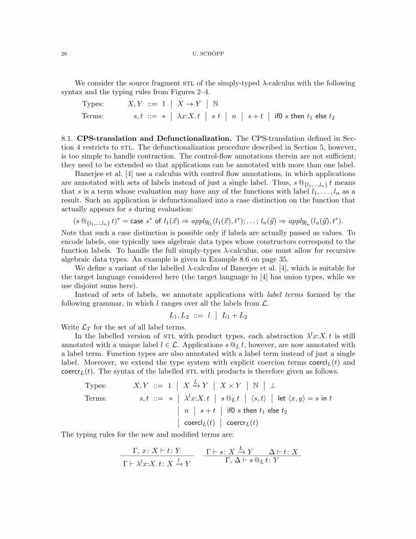
We consider the source fragment stl of the simply-typed λ-calculus with the followingsyntax and the typing rules from Figures 2–4.
Types: X,Y ::= 1∣∣ X → Y
∣∣ NTerms: s, t ::= ∗
∣∣ λx:X. t∣∣ s t ∣∣ n ∣∣ s+ t
∣∣ if0 s then t1 else t2
8.1. CPS-translation and Defunctionalization. The CPS-translation defined in Sec-tion 4 restricts to stl. The defunctionalization procedure described in Section 5, however,is too simple to handle contraction. The control-flow annotations therein are not sufficient;they need to be extended so that applications can be annotated with more than one label.
Banerjee et al. [4] use a calculus with control flow annotations, in which applicationsare annotated with sets of labels instead of just a single label. Thus, s@{l1,...,ln} t meansthat s is a term whose evaluation may have any of the functions with label l1, . . . , ln as aresult. Such an application is defunctionalized into a case distinction on the function thatactually appears for s during evaluation:
(s@{l1,...,ln} t)∗ = case s∗ of l1(~x)⇒ applyl1(l1(~x), t∗); . . . ; ln(~y)⇒ applyln(ln(~y), t∗).
Note that such a case distinction is possible only if labels are actually passed as values. Toencode labels, one typically uses algebraic data types whose constructors correspond to thefunction labels. To handle the full simply-types λ-calculus, one must allow for recursivealgebraic data types. An example is given in Example 8.6 on page 35.
We define a variant of the labelled λ-calculus of Banerjee et al. [4], which is suitable forthe target language considered here (the target language in [4] has union types, while weuse disjoint sums here).
Instead of sets of labels, we annotate applications with label terms formed by thefollowing grammar, in which l ranges over all the labels from L.
L1, L2 ::= l∣∣ L1 + L2
Write LT for the set of all label terms.In the labelled version of stl with product types, each abstraction λlx:X. t is still
annotated with a unique label l ∈ L. Applications s@L t, however, are now annotated witha label term. Function types are also annotated with a label term instead of just a singlelabel. Moreover, we extend the type system with explicit coercion terms coerclL(t) andcoercrL(t). The syntax of the labelled stl with products is therefore given as follows.
Types: X,Y ::= 1∣∣ X L−→ Y
∣∣ X × Y ∣∣ N∣∣ ⊥
Terms: s, t ::= ∗∣∣ λlx:X. t
∣∣ s@L t∣∣ 〈s, t〉 ∣∣ let 〈x, y〉 = s in t∣∣ n ∣∣ s+ t
∣∣ if0 s then t1 else t2∣∣ coerclL(t)∣∣ coercrL(t)
The typing rules for the new and modified terms are:
Γ, x : X ` t : YΓ ` λlx:X. t : X
l−→ Y
Γ ` s : XL−→ Y ∆ ` t : X
Γ, ∆ ` s@L t : Y
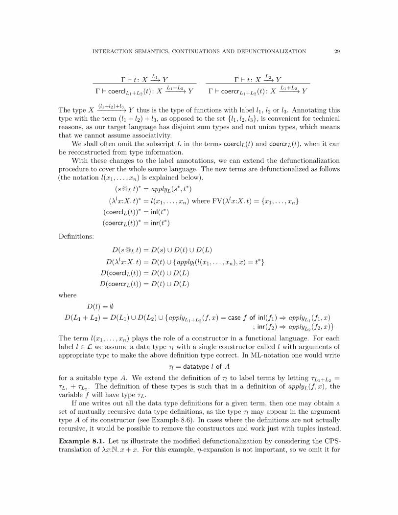
INTERACTION SEMANTICS, CONTINUATIONS AND DEFUNCTIONALIZATION 29
Γ ` t : X L1−→ Y
Γ ` coerclL1+L2(t) : XL1+L2−−−−→ Y
Γ ` t : X L2−→ Y
Γ ` coercrL1+L2(t) : XL1+L2−−−−→ Y
The type X(l1+l2)+l3−−−−−−→ Y thus is the type of functions with label l1, l2 or l3. Annotating this
type with the term (l1 + l2) + l3, as opposed to the set {l1, l2, l3}, is convenient for technicalreasons, as our target language has disjoint sum types and not union types, which meansthat we cannot assume associativity.
We shall often omit the subscript L in the terms coerclL(t) and coercrL(t), when it canbe reconstructed from type information.
With these changes to the label annotations, we can extend the defunctionalizationprocedure to cover the whole source language. The new terms are defunctionalized as follows(the notation l(x1, . . . , xn) is explained below).
(s@L t)∗ = applyL(s∗, t∗)
(λlx:X. t)∗ = l(x1, . . . , xn) where FV(λlx:X. t) = {x1, . . . , xn}(coerclL(t))∗ = inl(t∗)
(coercrL(t))∗ = inr(t∗)
Definitions:
D(s@L t) = D(s) ∪D(t) ∪D(L)
D(λlx:X. t) = D(t) ∪ {applyl(l(x1, . . . , xn), x) = t∗}D(coerclL(t)) = D(t) ∪D(L)
D(coercrL(t)) = D(t) ∪D(L)
where
D(l) = ∅D(L1 + L2) = D(L1) ∪D(L2) ∪ {applyL1+L2
(f, x) = case f of inl(f1)⇒ applyL1(f1, x)
; inr(f2)⇒ applyL2(f2, x)}
The term l(x1, . . . , xn) plays the role of a constructor in a functional language. For eachlabel l ∈ L we assume a data type τl with a single constructor called l with arguments ofappropriate type to make the above definition type correct. In ML-notation one would write
τl = datatype l of A
for a suitable type A. We extend the definition of τl to label terms by letting τL1+L2 =τL1 + τL2 . The definition of these types is such that in a definition of applyL(f, x), thevariable f will have type τL.
If one writes out all the data type definitions for a given term, then one may obtain aset of mutually recursive data type definitions, as the type τl may appear in the argumenttype A of its constructor (see Example 8.6). In cases where the definitions are not actuallyrecursive, it would be possible to remove the constructors and work just with tuples instead.
Example 8.1. Let us illustrate the modified defunctionalization by considering the CPS-translation of λx:N. x+ x. For this example, η-expansion is not important, so we omit it for
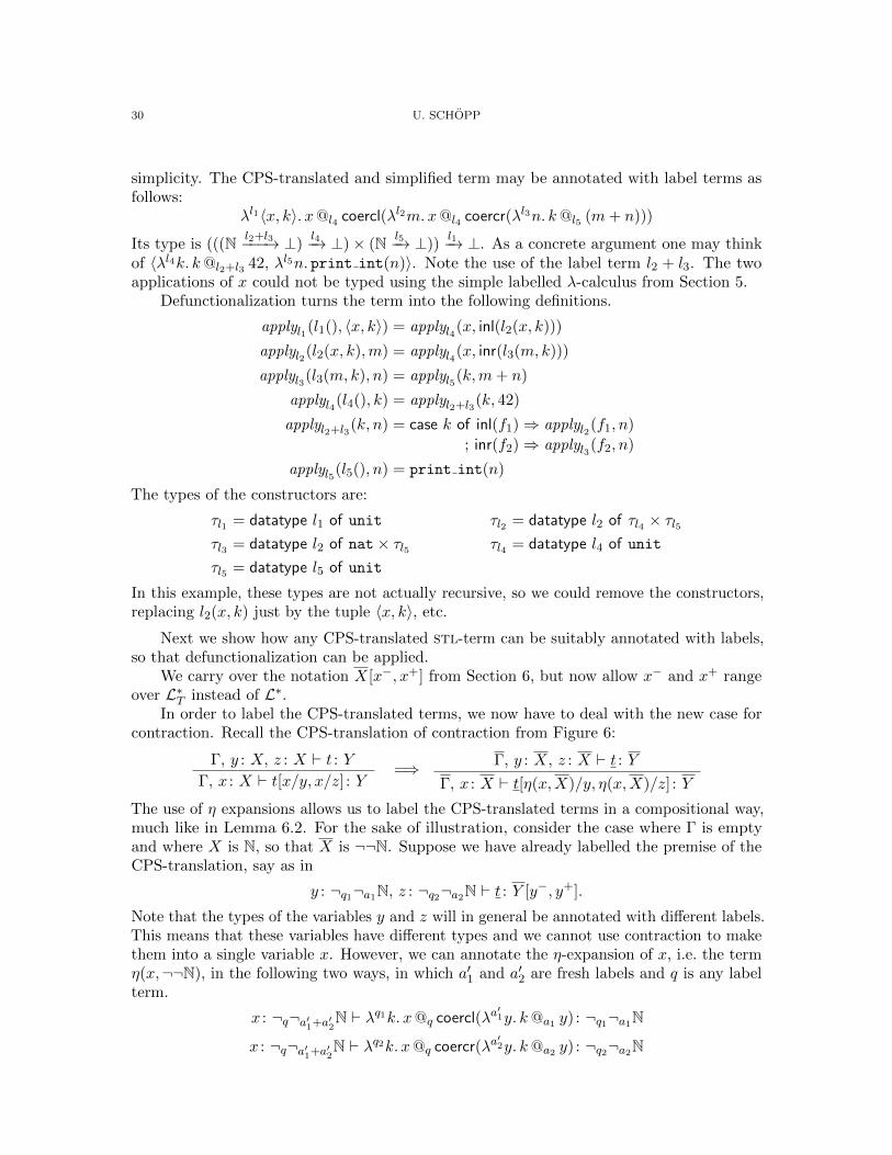
30 U. SCHOPP
simplicity. The CPS-translated and simplified term may be annotated with label terms asfollows:
λl1〈x, k〉. x@l4 coercl(λl2m.x@l4 coercr(λl3n. k@l5 (m+ n)))
Its type is (((N l2+l3−−−→ ⊥)l4−→ ⊥)× (N l5−→ ⊥))
l1−→ ⊥. As a concrete argument one may thinkof 〈λl4k. k@l2+l3 42, λl5n. print int(n)〉. Note the use of the label term l2 + l3. The twoapplications of x could not be typed using the simple labelled λ-calculus from Section 5.
Defunctionalization turns the term into the following definitions.
applyl1(l1(), 〈x, k〉) = applyl4(x, inl(l2(x, k)))
applyl2(l2(x, k),m) = applyl4(x, inr(l3(m, k)))
applyl3(l3(m, k), n) = applyl5(k,m+ n)
applyl4(l4(), k) = applyl2+l3(k, 42)
applyl2+l3(k, n) = case k of inl(f1)⇒ applyl2(f1, n)
; inr(f2)⇒ applyl3(f2, n)
applyl5(l5(), n) = print int(n)
The types of the constructors are:
τl1 = datatype l1 of unit τl2 = datatype l2 of τl4 × τl5τl3 = datatype l2 of nat× τl5 τl4 = datatype l4 of unit
τl5 = datatype l5 of unit
In this example, these types are not actually recursive, so we could remove the constructors,replacing l2(x, k) just by the tuple 〈x, k〉, etc.
Next we show how any CPS-translated stl-term can be suitably annotated with labels,so that defunctionalization can be applied.
We carry over the notation X[x−, x+] from Section 6, but now allow x− and x+ rangeover L∗T instead of L∗.
In order to label the CPS-translated terms, we now have to deal with the new case forcontraction. Recall the CPS-translation of contraction from Figure 6:
Γ, y : X, z : X ` t : YΓ, x : X ` t[x/y, x/z] : Y =⇒ Γ, y : X, z : X ` t : Y
Γ, x : X ` t[η(x,X)/y, η(x,X)/z] : Y
The use of η expansions allows us to label the CPS-translated terms in a compositional way,much like in Lemma 6.2. For the sake of illustration, consider the case where Γ is emptyand where X is N, so that X is ¬¬N. Suppose we have already labelled the premise of theCPS-translation, say as in
y : ¬q1¬a1N, z : ¬q2¬a2N ` t : Y [y−, y+].
Note that the types of the variables y and z will in general be annotated with different labels.This means that these variables have different types and we cannot use contraction to makethem into a single variable x. However, we can annotate the η-expansion of x, i.e. the termη(x,¬¬N), in the following two ways, in which a′1 and a′2 are fresh labels and q is any labelterm.
x : ¬q¬a′1+a′2N ` λq1k. x@q coercl(λa
′1y. k@a1 y) : ¬q1¬a1N
x : ¬q¬a′1+a′2N ` λq2k. x@q coercr(λa
′2y. k@a2 y) : ¬q2¬a2N

INTERACTION SEMANTICS, CONTINUATIONS AND DEFUNCTIONALIZATION 31
If we substitute the first term for y and the second term for z, then the resulting term is alabelled version of x : ¬q¬a′1+a′2N ` t[η(x,X)/y, η(x,X)/z] : Y [y−, y+], i.e. the conclusion ofthe CPS-translation of contraction. This outlines how we can substitute η-expansions of x,whereas we could not just substitute x for both y and z,
Of course, it remains to be shown that it is possible to find a labelling of the whole termeven when the type of x contains label terms, such as a′1 + a′2 instead of just fresh labels.Note that in the type of x we could not have put a single label in place of a′1 + a′2, as a′1and a′2 are the unique labels of two different abstractions.
The next two lemmas show that it is indeed always possible to label CPS-translatedterms appropriately. The following lemma first generalises the above labelling of η-expansionfrom N to an arbitrary type X. In the subsequent lemma, this is then used to deal with thecase of contraction as outlined above.
For any term t of labelled stl, we write |t| for the stl-term obtained by removing alllabel annotations and deleting all coercions. Likewise, we write |X| for the type obtainedby removing all label annotations. In the following lemma, we also extend the operation +to sequences of label terms: If r ∈ L∗T is L1 . . . Ln and r′ ∈ L∗T is L′1 . . . L
′n, then we write
r + r′ for (L1 + L′1) . . . (Ln + L′n).
Lemma 8.2. For any stl-type X there exists labels a′1, a′2, q1, q2 ∈ L∗ and labelled terms t1
and t2, such that |t1| = |t2| = η(x,X) and such that the judgements
x : X[q, a′1 + a′2] ` t1 : X[q1, a1] and x : X[q, a′1 + a′2] ` t2 : X[q2, a2]
are derivable for all label terms q, a1, a2 ∈ L∗T for which the types X[q, a′1 + a′2], X[q1, a1]
and X[q2, a2] are defined.
Proof. For any labelled type Y we define the list of label terms in positive/negative positions
in it: P (N) = P (⊥) = N(N) = N(⊥) = ε (the empty list), N(YL−→ Z) = LP (Y )N(Z) and
P (YL−→ Z) = N(Y )P (Z).
Informally, the η-expansion of a variable is such that the label terms in positive positionappear only as annotations of applications. There are no restrictions on the label terms inan application, so an η-expansion can be typed for arbitrary label terms in positive position.For the terms in negative position, there are constraints however. For each label termin a negative position the term contains a λ-abstraction. Since each abstraction must beannotated with a unique label, this leads to the constraint that the label terms in negativeposition can be obtained by coercion from the unique label of the abstraction in the term.
Formally, this can be expressed as follows: Let X be any stl-type and let X1 and X2
be labelled types with |X1| = |X2| = X. Then there exists a term t with |t| = η(x,X) suchthat x : X1 ` t : X2 is derivable whenever the list L1 . . . Ln := P (X1)N(X2) has the propertythat there are pairwise distinct labels l1, . . . , ln such that, for all i ∈ {1, . . . , n}, the label liis a sub-term of the label term Li.
The proof goes by induction on the type X. We spell out the case for function types.
• Case Y → Z. We have P (Y1L1−→ Z1)N(Y2
L2−→ Z2) = N(Y1)P (Z1)L2 P (Y2)N(Z2), bydefinition. The assumption on this list implies that P (Y2)N(Y1) has the property neededto apply the induction hypothesis to Y . Hence, there exists a labelled term ty with|ty| = η(y, Y ) and y : Y2 ` ty : Y1.
Likewise, the list P (Z1)N(Z2) is such that we can apply the induction hypothesis toobtain a term tz with |tz| = η(z, Z) and z : Z1 ` tz : Z2.

32 U. SCHOPP
If we define t′ = λl. tz[f @L1 ty/z], we therefore have |t′| = η(f, Y → Z) and f : Y1L1−→
Y1 ` t′ : Y2 l−→ Y2.By assumption, we know that we can choose l to be sub-term of L2, without violating
the constraint that each λ-abstraction must be uniquely identified by its label. The resulttherefore follows by applying coercions to t′.
The assertion now follows as a special case, where only coercions from a′1 to a′1 + a′2 andfrom a′2 to a′1 + a′2 are used.
With this lemma we can show that each derivation obtained by CPS-translation can betyped in the labelled variant of stl.
Lemma 8.3. If Γ ` t : X is derivable in stl, then there exist label terms x−, γ+ ∈ L∗T ,
such that, for all label terms x+, γ− ∈ L∗T for which Γ[γ−, γ+] and X[x−, x+] are defined,
the sequent Γ[γ−, γ+] ` t′ : X[x−, x+] is derivable for some labelled term t′ with |t′| = t.
Proof. The proof goes by induction on the derivation of Γ ` t : X. We consider representativecases. To simplify the notation we write just Γ[γ−, γ+] ` t : X[x−, x+] to express that thereexists a labelled term t′ with |t′| = t for which Γ[γ−, γ+] ` t′ : X[x−, x+] is derivable.
• Case ax. This case follows directly from Lemma 8.2.• Case →e. By induction hypothesis, there exist label terms y−x+1 , γ
+ ∈∗ L such that
Γ[γ−, γ+] ` s : X → Y [y−x+1 , y+x−1 ] is derivable for all label terms y+x−, γ− ∈ L∗T for
which all types in the sequent are defined. Also by induction hypothesis, there existslabel terms x−2 , δ
+ ∈ L∗T , such that for all label terms x+2 , δ− the sequent ∆[δ−, δ+] `
t : X[x−2 , x+2 ] is derivable. In particular, we can choose x+2 to be x+1 and x−1 to be x+2 and
obtain Γ[γ−, γ+], ∆[δ−, δ+] ` s t : Y [y−, y+]. Thus, we have shown that there exist labelterms y−, δ+γ+, such that the sequent is derivable for all label terms y+, δ−γ−, as wasrequired to show.• Case contr. By induction hypothesis, there exist label terms y−, γ+, x+1 , x
+2 such that
Γ[γ−, γ+], x1 : X[x−1 , x+1 ], x2 : X[x−2 , x
+2 ] ` t : Y [y−, y+] is derivable for all label terms
y+, γ−, x−1 , x−2 . By Lemma 8.2, there exist labels a′1, a
′2 ∈ L∗ and we can annotate η(x,X)
to become t1 and t2 so that that x : X[x−, a′1 +a′2] ` t1 : X[x−1 , x+1 ] and x : X[x−, a′1 +a′2] `
t2 : X[x−2 , x+2 ] are derivable.
We annotate the two copies of η(x,X) in the CPS-translation of contraction as t1 andt2.
Overall we obtain that there exist label terms y−, γ+, a′1 + a′2, such that
Γ[γ−, γ+], x : X[x−, a′1 + a′2] ` t[x/x1, x/x2] : Y [y−, y+]
is derivable for all y+, γ−, x−, which shows the assertion.
This lemma justifies the definition of CpsDefun also for stl: Given a derivation of Γ ` t : X,annotate its CPS-translation using the lemma, so that Γ[γ−, γ+] ` t : X[x−, x+] becomesderivable, and take CpsDefun(Γ ` t : X) := (x−γ+, D(t), x+γ−).
8.2. Interactive Interpretation. We now show how the Int-translation can be extendedto stl and how it relates to defunctionalization. To this end, we again consider a variant ofthe type system with subexponential annotations. We extend linexp to stlexp by addingsubexponential annotations to the contraction rule and by adding a new rule struct for
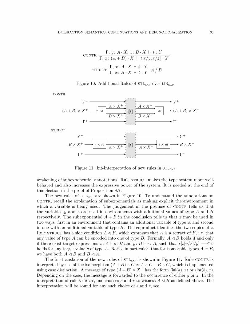
INTERACTION SEMANTICS, CONTINUATIONS AND DEFUNCTIONALIZATION 33
Γ, y : A ·X, z : B ·X ` t : Ycontr
Γ, x : (A+B) ·X ` t[x/y, x/z] : Y
Γ, x : A ·X ` t : Ystruct A / B
Γ, x : B ·X ` t : Y
Figure 10: Additional Rules of stlexp over linexp
Y −
Y +
A×X−
contr
JtK 'B ×X−
(A + B) ×X−'A×X+
B ×X+
(A + B) ×X+
struct
JtK s× idr × idA×X−A×X+
Y +
B ×X−B ×X+
Y −
Γ−Γ+
Γ+ Γ−
Figure 11: Int-Interpretation of new rules in stlexp
weakening of subexponential annotations. Rule struct makes the type system more well-behaved and also increases the expressive power of the system. It is needed at the end ofthis Section in the proof of Proposition 8.7.
The new rules of stlexp are shown in Figure 10. To understand the annotations oncontr, recall the explanation of subexponentials as making explicit the environment inwhich a variable is being used. The judgement in the premise of contr tells us thatthe variables y and z are used in environments with additional values of type A and Brespectively. The subexponential A + B in the conclusion tells us that x may be used intwo ways: first in an environment that contains an additional variable of type A and secondin one with an additional variable of type B. The coproduct identifies the two copies of x.Rule struct has a side condition ACB, which expresses that A is a retract of B, i.e. thatany value of type A can be encoded into one of type B. Formally, ACB holds if and onlyif there exist target expressions x : A ` s : B and y : B ` r : A, such that r[s[v/x]/y] −→∗ vholds for any target value v of type A. Notice in particular, that for isomorphic types A ' B,we have both ACB and B CA.
The Int-translation of the new rules of stlexp is shown in Figure 11. Rule contr isinterpreted by use of the isomorphism (A+B)×C ' A×C +B×C, which is implementedusing case distinction. A message of type (A+B)×X+ has the form 〈inl(a), x〉 or 〈inr(b), x〉.Depending on the case, the message is forwarded to the occurrence of either y or z. In theinterpretation of rule struct, one chooses s and r to witness ACB as defined above. Theinterpretation will be sound for any such choice of s and r, see.

34 U. SCHOPP
8.3. Relating the Translations. We have now defined two translations from stlexp tothe target language. To relate them, we begin by spelling out a simple example to illustratethat both translations treat contraction in the same way.
Example 8.4. Consider again the source term λx:N. x+ x. Its Int-interpretation may bedepicted as follows.
N
nat×N−nat×N+
unit×N−N−
(unit+nat)×N−
unit×N+
l1 l5
l4l2
l3(unit+nat)×N+'
add
q′
q′′'a′
a′′a′+a′′
The box labelled add is defined as in the Introduction, up to uses of the isomorphismunit×N+ ' N+. The interpretation of rule contr inserts the two boxes labelled ', whichdenote the canonical isomorphism of their type.
This program implements the term λx:N. x+ x as follows: To compute the result ofthe function when applied to the actual argument 42, one connects the output of type(unit + nat)×N− to the input of type (unit + nat)×N+ such that when the value 〈k′, 〈〉〉arrives at the output port, then the value 〈k′, 42〉 is fed back to the input port.
Consider now the CPS-translation of the term λx:N. x+ x. If we omit the η-expansionsin the translation of variables for simplicity, then we obtain the term
λl1〈x, k〉. t1 @q′ (λl2m. t2 @q′′ (λ
l3n. k@l5 (m+ n))) (8.1)
of type (((N a′+a′′−−−−→ ⊥)q′−→ ⊥) × (N l5−→ ⊥))
l1−→ ⊥, wherein t1 and t2 are the η-expansions
(λq′k. x@l4 coercl(λa
′n. k@l2 n)) and (λq
′′k. x@l4 coercr(λa
′′n. k@l3 n)) respectively. These
two η-expansions come from the CPS-translation of contraction. Defunctionalization of theterm in (8.1) leads to the equations
applyl1(〈〉, 〈x, k〉) = applyq′(q′(x), l2(x, k))
applyl2(l2(x, k),m) = applyq′′(q′′(x), l3(m, k))
applyl3(l3(m, k), n) = applyl5(k,m+ n),
and the subterms t1 and t2 add the following equations:
applyq′(q′(x), k) = applyl4(x, inl(a′(k))) applya′(a
′(k), n) = applyl2(k, n)
applyq′′(q′′(x), k) = applyl4(x, inr(a′′(k))) applya′′(a
′′(k), n) = applyl3(k, n)
applya′+a′′(k, n) = case k of inl(f1)⇒ applya′(f1, n)
; inr(f2)⇒ applya′′(f2, n)(8.2)
In order to understand how this program works, it is perhaps again useful to apply theabove term to the argument 〈λl4k. k@a′+a′′ 42, λl5n. print int(n)〉. Defunctionalizationthen yields two additional equations.
applyl4(〈〉, k) = applya′+a′′(k, 42)
applyl5(〈〉, n) = print int(n)
Note how this program computes the result in the same way as the one obtained by Int-interpretation above. Both programs have the same skeleton. The points corresponding tothe apply-equations are labelled in the Int-interpretation above. Notice in particular how

INTERACTION SEMANTICS, CONTINUATIONS AND DEFUNCTIONALIZATION 35
the equations (8.2) that come from the η-expansion in the CPS-translation of contractioncorrespond to the isomorphisms added by the interpretation of rule contr in the Int-interpretation.
Proposition 8.5. For any Γ ` t : X derivable in stlexp, there exists a target programInt(Γ ` t : X) that is a representative of the Int-interpretation of the derivation of the sequentand that has the same skeleton as CpsDefun(Γ ` t : X).
Proof. The proof goes by induction on the derivation, just as for Proposition 7.2. The onlynew case is that for contraction. To handle this case, consider the defunctionalization of thetwo η-expansions x : X[q, a′1 + a′2] ` t1 : X[q1, a1] and x : X[q, a′1 + a′2] ` t2 : X[q2, a2] fromLemma 8.2. Let us write q1(i) for the i-th label term in the list q1, and likewise for theother lists. Observe that the defunctionalization of the terms t1 and t2 yield equations ofthe following shape for all possible indices i:
applyq1(i)(−,−) = applyq(i)(−, inl(−))
applyq2(i)(−,−) = applyq(i)(−, inr(−))
apply(a′1+a′2)(i)(x,−) = case x of inl(y)⇒ applya1(i)(y,−)
; inr(z)⇒ applya2(i)(z,−)
applya′1(i)(−,−) = applya1(i)(−,−)
These equations have the same skeleton as an appropriate choice of equations forthe Int-interpretation of rule contr. One can thus choose a representative of the Int-interpretation having the same skeleton as the program obtained from CPS-translation anddefunctionalization.
The proposition establishes a relation of the Int-interpretation and CPS-translationfollowed by defunctionalization for terms typeable in stlexp. An obvious question is howmuch of stl is covered by this result. In the rest of this section we show that with rulestruct and recursive types in the target language, in fact any stl-term can be typed instlexp.
We first give an example to show how recursive target types appear in the two translations.When we discussed defunctionalization for stl, we have already remarked that recursive typesare needed in the target language to treat the full simply-typed λ-calculus. The followingexample (i) illustrates the use of struct and recursive types in stlexp; and (ii) shows thatrecursive types may appear even in the defunctionalization of the simply-typed λ-calculus.
Example 8.6. An example that illustrates why without recursive types in the targetlanguage not every stl-term would be typeable in stlexp is the application t s, wheret = λg. g (λx. g (λy.x)) and s = λf. f (f (λx.x)). The terms t and s can be given types(unit + α) · (α · (α ·X → X)→ X)→ X and (unit + β) · (β ·X → X)→ X respectively,for a certain type X. In these types the subexponential annotations have been simplifiedusing only the isomorphism (−)× unit ' (−), which can be used by means of rule struct.
Without recursive types in the target language, the application t s could not be typed, asthis would require us to unify (unit+β) ·(β ·X → X)→ X with α ·(α ·X → X)→ X, whichwould require unifying β and unit + β. With recursive types, however, we can simply letB := µβ. unit+β and instantiate the type variable β to be B. Since we have unit+BCB,we can use rule struct to give s the type B · (B ·X → X)→ X and with this give t s thetype X .
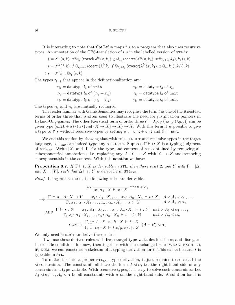
36 U. SCHOPP
It is interesting to note that CpsDefun maps t s to a program that also uses recursivetypes. An annotation of the CPS-translation of t s in the labelled version of stl is:
t = λl1〈g, k〉. g@l4 〈coercl(λl2〈x, k1〉. g@l4 〈coercr(λl3〈y, k3〉. x@l5+l6 k3), k1〉), k〉s = λl4〈f, k〉. f @l2+l3 〈coercl(λl5k2. f @l2+l3 〈coercr(λl6〈x, k1〉. x@l8 k1), k2〉), k〉
t s = λl7k. t@l1 〈s, k〉The types τ(−) that appear in the defunctionalization are:
τl1 = datatype l1 of unit τl2 = datatype l2 of τl4
τl3 = datatype l3 of (τl5 + τl6) τl4 = datatype l4 of unit
τl5 = datatype l5 of (τl2 + τl3) τl6 = datatype l6 of unit
The types τl3 and τl5 are mutually recursive.The reader familiar with Game Semantics may recognise the term t as one of the Kierstead
terms of order three that is often used to illustrate the need for justification pointers inHyland-Ong-games. The other Kierstead term of order three t′ = λg. g (λx. g (λy.y)) can begiven type (unit+ α) · (α · (unit ·X → X)→ X)→ X. With this term it is possible to givea type to t′ s without recursive types by setting α := unit + unit and β := unit.
We end this section by showing that with rule struct and recursive types in the targetlanguage, stlexp can indeed type any stl-term. Suppose Γ ` t : X is a typing judgmentof stlexp. Write |X| and |Γ| for the type and context of stl obtained by removing allsubexponential annotations, i.e. replacing any A · Y → Z with Y → Z and removingsubexponentials in the context. With this notation we have:
Proposition 8.7. If Γ ` t : X is derivable in stl, then there exist ∆ and Y with Γ = |∆|and X = |Y |, such that ∆ ` t : Y is derivable in stlexp.
Proof. Using rule struct, the following rules are derivable.
ax unitC α1x : α1 ·X ` x : X
Γ ` s : A ·X → Y x1 : A1 ·X1, . . . , xn : An ·Xn ` t : X→eA×A1 C α1, . . . ,A×An C αnΓ, x1 : α1 ·X1, . . . , xn : αn ·Xn ` s t : Y
Γ ` s : N x1 : A1 ·X1, . . . , xn : An ·Xn ` t : Nadd
nat×A1 C α1, . . . ,nat×An C αnΓ, x1 : α1 ·X1, . . . , xn : αn ·Xn ` s+ t : N
Γ, y : A ·X, z : B ·X ` t : Zcontr (A+B) C α1
Γ, x : α1 ·X ` t[x/y, x/z] : Z
We only need struct to derive these rules.If we use these derived rules with fresh target type variables for the αi and disregard
the C-side-conditions for now, then together with the unchanged rules weak, exch →i,if, num, we can construct a skeleton of a typing derivation for t. This exists because t istypeable in stl.
To make this into a proper stlexp type derivation, it just remains to solve all theC-constraints. The constraints all have the form A C α, i.e. the right-hand side of anyconstraint is a type variable. With recursive types, it is easy to solve such constraints: LetA1 C α, . . . , An C α be all constraints with α on the right-hand side. A solution for it is
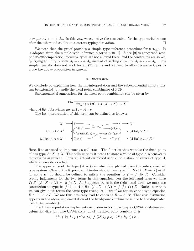
INTERACTION SEMANTICS, CONTINUATIONS AND DEFUNCTIONALIZATION 37
α := µα.A1 + · · ·+An. In this way, we can solve the constraints for the type variables oneafter the other and so obtain a correct typing derivation.
We note that the proof provides a simple type inference procedure for stlexp. Itis adapted from the simple type inference algorithm in [9]. Since [9] is concerned withlogspace-computation, recursive types are not allowed there, and the constraints are solvedby trying to unify α with A1 + · · · + An instead of setting α := µα.A1 + · · · + An. Thissimple heuristic does not work for all stl terms and we need to allow recursive types toprove the above proposition in general.
9. Recursion
We conclude by explaining how the Int-interpretation and the subexponential annotationscan be extended to handle the fixed point combinator of PCF.
Subexponential annotations for the fixed-point combinator can be given by
fixfixX : (A list) · (A ·X → X)→ X
where A list abbreviates µα. unit +A× α.The Int-interpretation of this term can be defined as follows:
(A list)×X+
X−
〈nil, a〉〈cons(x, l), a〉
〈l, x, q〉 〈l, x, a〉
〈nil, q〉〈cons(x, l), q〉
q a
(A list)×A×X−
(A list)×X−
X+
(A list)×A×X+
Here, lists are used to implement a call stack. The function that we take the fixed pointof has type A ·X → X. This tells us that it needs to store a value of type A whenever itrequests its argument. Thus, an activation record should be a stack of values of type A,which we encode as a list.
The appearance of the type (A list) can also be explained from the subexponentialtype system. Clearly, the fixpoint combinator should have type fix : B · (A ·X → X)→ Xfor some B. It should be defined to satisfy the equation fix f = f (fix f). Considertyping judgements for the two terms in this equation. For the left-hand term we havef : B · (A ·X → X) ` fix f : X. As f appears twice in the right-hand term, we must usecontraction to type it: f : (1 + A × B) · (A · X → X) ` f (fix f) : X. Notice now thatwe can give both terms the same type (using struct) if we can solve the type equationB ' 1 +A×B. We are thus naturally lead to choosing B := A list. That case distinctionappears in the above implementation of the fixed-point combinator is due to the duplicateduse of the variable f .
The Int-interpretation implements recursion in a similar way as CPS-translation anddefunctionalization. The CPS-translation of the fixed point combinator is
λq1〈f, k〉. fixX (λq4g. λk1. f 〈λq3k2. g k2, λq2x. k1 x〉) k .

38 U. SCHOPP
A possible defunctionalization (without using control flow information) of this term is:
apply(q1(), 〈f, k〉) = apply(q4(f), k) apply(q2(k1), x) = apply(k1, x)
apply(q3(g), k2) = apply(g, k2) apply(q4(f), k1) = apply(f, 〈q3(q4(f)), q2(k1)〉)Informally, the first three definitions to correspond to the inputs of the Int-interpretationabove. A call to apply(q1(), 〈f, k〉) starts the recursion, a call to apply(q2(k1), x) correspondsto the step function (that the fixed point is taken of) returning a result, and a call toapply(q3(g), k2) corresponds to the step function requesting its argument. The final equationdoes not contribute to the external interface of the program and is used to implement thefixed point. The call stack, which above is encoded using lists, appears more implicitly inthe continuations here.
10. Conclusion
We have observed that the non-standard compilation methods based on computation byinteraction are closely related to CPS-translation and defunctionalization. The interpretationin an interactive model may be regarded as a simple direct description of the combination ofCPS-translation, defunctionalization and a final optimisation of arguments. It may be seenas a simple nameless formulation of a combined CPS-translation and defunctionalizationand it provides an alternative way of encoding continuations.
We have seen in this paper that working out the technical details of defunctionalizationwith explicit labels can become quite technical. The interactive interpretation admits a high-level description that abstracts from implementation details. Interactive model constructionsmay perhaps be useful in simplifying uses of defunctionalization. In the other direction,being aware that interactive models are related to standard compilation methods may helpto improve non-standard compilation schemes based on interactive methods, such as [14, 8].We may hope that some of the many existing techniques for compiler implementation canbe adapted usefully to the non-standard schemes.
Types with subexponential annotations, in this form originally introduced in IntML [8],provide a logical account for the issues of managing value environments that are inherent todefunctionalization. With subexponential annotations, the type of a higher-order term fullyspecifies the interface of the target program obtained from it. The type system containsenough information in order to give a fully compositional definition of the translation to thetarget language.
The subexponential type system makes explicit issues that appear with defunctional-ization and separate compilation. For example, in order to suppose we want to compile afunction f : A ·X → Y separately from the rest of the program. Then one may compilethe main program f : B · (A · X → Y ) ` t : Z and ` f : A · X → Y separately. A linkercan combine the resulting two programs knowing only their types. Of course, the problemsassociated with defunctionalization and separate compilation do not just disappear. Suppose,for example, we only know the term f , but not the program t in which it will be used.Suppose further that X has the form C · N → N. Then the choice of the subexponentialannotation C will limit which arguments f can be applied to; f can only be applied toarguments of type D · N→ N with D C C. Choosing C without knowledge of t is possible,for example, if the target language has a type Heap with DCHeap for any type D (anythingcan be stored on the heap). Then one may simply choose C to be Heap. This is not theonly possible choice; for performance reasons one may consider performing a more precise
INTERACTION SEMANTICS, CONTINUATIONS AND DEFUNCTIONALIZATION 39
analysis in a linker or similar. The point is that the subexponential type system allows us toexpress such issues at a high level and to apply different possible solutions. Another examplefor this point is the explanation of the appearance of recursive target types in Section 8,which was given in terms of subexponential type annotations.
Subexponentials refine the exponentials in AJM games [2], where !X is implementedusing ω ·X, where ω is a type of unbounded natural numbers. If we had used full exponentialsin the Int-interpretation above, then we would have obtained a compilation method thatencodes function values as values in ω, which is akin to storing closures on the heap.Subexponentials give us more control to avoid such encodings where unnecessary. Thesubexponential type system in this paper has its origin in Bounded Linear Logic [18, 38].It is also similar to the type system for Syntactic Control of Concurrency (SCC) [15]. Amain difference appears to be that while SCC controls the number of program threads,subexponentials account for both the threads and their local data.
The observation that there is a connection between game models and continuations isnot new. It appears, for example, in Levy’s work on a jump-with-argument calculus [26]and in Mellies work on tensorial logic [29]. Connections of game models to compilation havealso been made, e.g. [30]. Furthermore, it is well-known that continuation passing is relatedto message passing, see e.g. [41]. However, we are not aware of work that makes explicit aconnection to defunctionalization.
We believe that the connection between game models and machine languages deservesto be better known and studied further. The call traces in this paper, for example, shouldhave the same status as plays in Game Semantics. This suggests that techniques fromGame Semantics help to analyse the possible traces of compiled machine code. For Java-likelanguages, there is recent work that connects fully abstract trace semantics [24] and GameSemantic models [33]. We hope that similar connections can be identified for the traces ofmachine code generated by compilers.
Work on concurrency and process calculus emphasises the interactive nature of compu-tation. Milner’s translation of the λ-calculus in the π-calculus [31] can be understood as aCPS-translation [37]. This connection was made more than once: see [37, §10] for historicalnotes. The interactive model that we have studied in this paper can be seen as a very staticform of communicating processes, without process mobility or channel reconfiguration. InMilner’s translation, channel names identify continuations and these are passed aroundexplicitly. We have seen in this paper that by taking into account control flow information,it is possible to avoid passing continuations names, as they can be determined statically.It is an interesting direction for further work to find out if Milner’s translation relates toCPS-translation and defunctionalization without control flow information. In this direction,it may perhaps be possible to connect to the interesting results of Berger et al. [5].
In further work, we should like to understand possible connections to Danvy’s work ondefunctionalized interpreters [11], or more generally to work on continuations and abstractmachines, e.g. [10, 40]. A relation is not obvious: Danvy considers the defunctionalization ofparticular implementations of interpreters, while here we show that the whole compilationitself may be described extensionally by the Int construction.
In another direction, an interactive view of CPS-translation and defunctionalization mayalso help in identifying mathematical structure of efficient compilation methods. In particular,capturing call-by-value defunctionalizing compilation, perhaps similar to [7], should beinteresting. Other interesting issues are efficient separate compilation and polymorphism:

40 U. SCHOPP
the interpretation in Int(T) is compositional and polymorphism can also be accountedfor [38].
Finally, this paper clarifies the definition of IntML [8], which was introduced to capturelogspace. In [8] we observed that IntML supports control operators, such as callcc, buttheir status remained somewhat unclear. It now turns out that the callcc combinator of [8]may be understood as the defunctionalization of a standard CPS implementation of callcc.
Acknowledgements. I would like to thank the anonymous referees for their constructivefeedback and suggestions, which helped to improve the presentation of the results.
References
[1] Samson Abramsky, Esfandiar Haghverdi, and Philip J. Scott. Geometry of interaction and linearcombinatory algebras. Mathematical Structures in Computer Science, 12(5):625–665, 2002.
[2] Samson Abramsky, Radha Jagadeesan, and Pasquale Malacaria. Full abstraction for PCF. Informationand Computation, 163(2):409–470, 2000.
[3] Andrew W. Appel. Compiling with Continuations. Cambridge University Press, 1992.[4] Anindya Banerjee, Nevin Heintze, and Jon G. Riecke. Design and correctness of program transformations
based on control-flow analysis. In Naoki Kobayashi and Benjamin C. Pierce, editors, Theoretical Aspectsof Computer Software, TACS 2001, volume 2215 of Lecture Notes in Computer Science, pages 420–447.Springer, 2001.
[5] Martin Berger, Kohei Honda, and Nobuko Yoshida. Sequentiality and the π-calculus. In SamsonAbramsky, editor, Typed Lambda Calculi and Applications, TLCA 2001, volume 2044 of Lecture Notesin Computer Science, pages 29–45. Springer, 2001.
[6] Andreas Blass. A game semantics for linear logic. Annals of Pure and Applied Logic, 56(1-3):183–220,1992.
[7] Henry Cejtin, Suresh Jagannathan, and Stephen Weeks. Flow-directed closure conversion for typedlanguages. In Gert Smolka, editor, European Symposium on Programming, ESOP 2000, volume 1782 ofLecture Notes in Computer Science, pages 56–71. Springer, 2000.
[8] Ugo Dal Lago and Ulrich Schopp. Functional programming in sublinear space. In Andrew D. Gordon,editor, European Symposium on Programming, ESOP 2010, volume 6012 of Lecture Notes in ComputerScience, pages 205–225. Springer, 2010.
[9] Ugo Dal Lago and Ulrich Schopp. Type inference for sublinear space functional programming. In KazunoriUeda, editor, Asian Symposium on Programming Languages and Systems, APLAS 2010, volume 6461 ofLecture Notes in Computer Science, pages 376–391. Springer, 2010.
[10] Vincent Danos, Hugo Herbelin, and Laurent Regnier. Game semantics and abstract machines. In Logicin Computer Science, LICS 1996, pages 394–405. IEEE Computer Society, 1996.
[11] Olivier Danvy. Defunctionalized interpreters for programming languages. In James Hook and PeterThiemann, editors, International Conference on Functional Programming, ICFP 2008, pages 131–142.ACM, 2008.
[12] Olle Fredriksson and Dan R. Ghica. Seamless distributed computing from the geometry of interaction.In Catuscia Palamidessi and Mark Dermot Ryan, editors, Trustworthy Global Computing, TGC 2012,volume 8191 of Lecture Notes in Computer Science, pages 34–48. Springer, 2012.
[13] Olle Fredriksson and Dan R. Ghica. Abstract machines for game semantics, revisited. In Logic InComputer Science, LICS 2013, pages 560–569. IEEE Computer Society, 2013.
[14] Dan R. Ghica. Geometry of synthesis: a structured approach to VLSI design. In Martin Hofmann andMatthias Felleisen, editors, Principles of Programming Languages, POPL 2007, pages 363–375. ACM,2007.
[15] Dan R. Ghica, Andrzej S. Murawski, and C.-H. Luke Ong. Syntactic control of concurrency. TheoreticalComputer Science, 350(2-3):234–251, 2006.
[16] Dan R. Ghica, Alex I. Smith, and Satnam Singh. Geometry of synthesis IV: compiling affine recursion intostatic hardware. In Manuel M. T. Chakravarty, Zhenjiang Hu, and Olivier Danvy, editors, InternationalConference on Functional Programming, ICFP 2011, pages 221–233. ACM, 2011.

INTERACTION SEMANTICS, CONTINUATIONS AND DEFUNCTIONALIZATION 41
[17] Jean-Yves Girard. Towards a geometry of interaction. In J. W. Gray and A. Scedrov, editors, Categoriesin Computer Science and Logic, pages 69–108. American Mathematical Society, 1989.
[18] Jean-Yves Girard, Andre Scedrov, and Philip J. Scott. Bounded linear logic: a modular approach topolynomial-time computability. Theoretical Computer Science, 97:1–66, 1992.
[19] Masahito Hasegawa. On traced monoidal closed categories. Mathematical Structures in Computer Science,19(2):217–244, 2009.
[20] Ichiro Hasuo and Naohiko Hoshino. Semantics of higher-order quantum computation via geometry ofinteraction. In Logic in Computer Science, LICS 2011, pages 237–246. IEEE Computer Society, 2011.
[21] Martin Hofmann and Thomas Streicher. Continuation models are universal for lambda-mu-calculus. InLogic in Computer Science, LICS 1997, pages 387–395. IEEE Computer Society, 1997.
[22] J. M. E. Hyland and C.-H. Luke Ong. Pi-calculus, dialogue games and PCF. In Functional ProgrammingLanguages and Computer Architecture, FPCA 1995, pages 96–107, 1995.
[23] J. M. E. Hyland and C.-H. Luke Ong. On full abstraction for PCF: I, II, and III. Information andComputation, 163:285–408, December 2000.
[24] Alan Jeffrey and Julian Rathke. Java jr: Fully abstract trace semantics for a core Java language. InShmuel Sagiv, editor, European Symposium on Programming, ESOP 2005, volume 3444 of Lecture Notesin Computer Science, pages 423–438. Springer, 2005.
[25] Andre Joyal, Ross Street, and Dominic Verity. Traced monoidal categories. Mathematical Proceedings ofthe Cambridge Philosophical Societ, 119(3):447–468, 1996.
[26] Paul Blain Levy. Call-By-Push-Value: A Functional/Imperative Synthesis, volume 2 of SemanticsStructures in Computation. Springer, Berlin, Heidelberg, 2004.
[27] Paul Lorenzen. Ein dialogisches Konstruktivitatskriterium. Infinitistic Methods, 1961.[28] Ian Mackie. The geometry of interaction machine. In Ron K. Cytron and Peter Lee, editors, Principles
of Programming Languages, POPL 1995, pages 198–208. ACM, 1995.[29] Paul-Andre Mellies. Game semantics in string diagrams. In Logic in Computer Science, LICS 2012,
pages 481–490. IEEE, 2012.[30] Paul-Andre Mellies and Nicolas Tabareau. An algebraic account of references in game semantics.
Electronic Notes in Theoretical Computer Science, 249:377–405, 2009.[31] Robin Milner. Functions as processes. Mathematical Structures in Computer Science, 2(2):119–141, 1992.[32] Andrzej S. Murawski and Nikos Tzevelekos. Full abstraction for Reduced ML. Annals of Pure and
Applied Logic, 164(11):1118–1143, 2013.[33] Andrzej S. Murawski and Nikos Tzevelekos. Game semantics for interface middleweight java. In Suresh
Jagannathan and Peter Sewell, editors, Principles of Programming Languages, POPL 2014, pages517–528. ACM, 2014.
[34] Benjamin C. Pierce. Types and programming languages. MIT Press, 2002.[35] Gordon D. Plotkin. Call-by-name, call-by-value and the lambda-calculus. Theoretical Computer Science,
1(2):125–159, 1975.[36] John C. Reynolds. Definitional interpreters for higher-order programming languages. In Proceedings of
the ACM annual conference - Volume 2, ACM ’72, pages 717–740. ACM, 1972.[37] Davide Sangiorgi. From lambda to pi; or, rediscovering continuations. Mathematical Structures in
Computer Science, 9(4):367–401, 1999.[38] Ulrich Schopp. Stratified bounded affine logic for logarithmic space. In Logic in Computer Science, LICS
2007, pages 411–420. IEEE, 2007.[39] Zhong Shao and Andrew W. Appel. Efficient and safe-for-space closure conversion. ACM Transactions
on Programming Languages and Systems, 22(1):129–161, 2000.[40] Thomas Streicher and Bernhard Reus. Classical logic, continuation semantics and abstract machines.
Journal of Functional Programming, 8(6):543–572, 1998.[41] Hayo Thielecke. Categorical Structure of Continuation Passing Style. PhD thesis, The University of
Edinburgh, 1997.[42] Akira Yoshimizu, Ichiro Hasuo, Claudia Faggian, and Ugo Dal Lago. Measurements in proof nets as
higher-order quantum circuits. In Zhong Shao, editor, European Symposium on Programming, ESOP2014, volume 8410 of Lecture Notes in Computer Science, pages 371–391. Springer, 2014.
This work is licensed under the Creative Commons Attribution-NoDerivs License. To viewa copy of this license, visit http://creativecommons.org/licenses/by-nd/2.0/ or send aletter to Creative Commons, 171 Second St, Suite 300, San Francisco, CA 94105, USA, orEisenacher Strasse 2, 10777 Berlin, Germany