On the Patterns of Wind-Power Input to the Ocean...

On the Patterns of Wind-Power Input to the Ocean Circulation

FABIEN ROQUET AND CARL WUNSCH

Department of Earth, Atmosphere and Planetary Science, Massachusetts Institute of Technology, Cambridge, Massachusetts

GURVAN MADEC

Laboratoire d’Oceanographie Dynamique et de Climatologie, Paris, France

(Manuscript received 1 February 2011, in final form 12 July 2011)

ABSTRACT

Pathways of wind-power input into the ocean general circulation are analyzed using Ekman theory. Direct

rates of wind work can be calculated through the wind stress acting on the surface geostrophic flow. However,

because that energy is transported laterally in the Ekman layer, the injection into the geostrophic interior is

actually controlled by Ekman pumping, with a pattern determined by the wind curl rather than the wind itself.

Regions of power injection into the geostrophic interior are thus generally shifted poleward compared to

regions of direct wind-power input, most notably in the Southern Ocean, where on average energy enters the

interior 108 south of the Antarctic Circumpolar Current core. An interpretation of the wind-power input to

the interior is proposed, expressed as a downward flux of pressure work. This energy flux is a measure of the

work done by the Ekman pumping against the surface elevation pressure, helping to maintain the observed

anomaly of sea surface height relative to the global-mean sea level.

1. Introduction

The wind stress, along with the secondary input from

tides, provides the main source of mechanical energy

compensating the continuous loss to friction (Wunsch

and Ferrari 2004). Knowledge of the distribution and

fate of the wind stress power input to the ocean is es-

sential for the understanding of the ocean circulation

and its variability. Among the wide range of ocean move-

ments induced by the wind forcing, the large-scale ocean

general circulation is of special interest. This paper aims

at better understanding where and how wind powers

the ocean general circulation.

Several global estimates of power input to the ocean

general circulation have been made, ranging between

about 0.75 and 1 TW (Wunsch 1998; Huang et al. 2006;

von Storch et al. 2007; Hughes and Wilson 2008; Scott and

Xu 2009). Other sources of wind-power input are com-

paratively large, such as the power input to the ageo-

strophic circulation (about 3 TW; Wang and Huang 2004a)

or the input to surface gravity waves (601 TW; Wang

and Huang 2004b), but they are not directly related to

the interior flow.

Three methods for determining the local rate of wind-

power input to the ocean general circulation have been

proposed in the literature: 1) the direct rate of work on

the geostrophic circulation (Stern 1975); 2) the rate at

which the Ekman transport crosses the surface pressure

gradient (Fofonoff 1981); and 3) the rate at which Ekman

pumping generates potential energy in a stratified fluid

(Gill et al. 1974). Only the first form has been used to

make global estimates. That these three views must be

equivalent was known to these authors, but exactly how

that equivalence comes about is not obvious. Note, for

example, that the two first forms depend on the wind

stress but the third depends on the wind stress curl, and

thus one expects their spatial patterns to be different.

In this paper, two alternative expressions for the rate

of wind-power input into the geostrophic interior are

derived. To illustrate the concepts developed later, Fig. 1

displays estimates of these two expressions for the South-

ern Ocean, which were made by methods to be described

later. The first maps corresponds to the direct rate of

wind-power input to the geostrophic circulation (Stern

and Fofonoff views), whereas the second map (somewhat

Corresponding author address: Fabien Roquet, Department of

Earth, Atmosphere and Planetary Science, Massachusetts Institute

of Technology, Cambridge, MA 02139.

E-mail: [email protected]

2328 J O U R N A L O F P H Y S I C A L O C E A N O G R A P H Y VOLUME 41

DOI: 10.1175/JPO-D-11-024.1

� 2011 American Meteorological Society

closer to the Gill view) represents the input of pressure

work injected into the interior ocean. Although the

representations have different spatial patterns, they are

equivalent in the sense that their integrals over the

global ocean are strictly identical, as will be shown.

After presenting a theoretical description of wind-

related energy pathways and their physical significance,

realistic estimates will be proposed for the global ocean.

A more detailed examination will then be undertaken

of the Southern Ocean, which has the most conspicu-

ous importance to the energetics. Because the physics

employed here are elementary—geostrophic flows and

Ekman layers—the chief goal is insight into energy path-

ways as a means to better understanding rather than any

new general circulation properties.

2. The rate of wind work on the interior

a. Ekman pumping

As has been clear since the work of Stommel (1957),

Ekman pumping of the geostrophic interior represents

a major control on the general circulation. To establish

a notation, consider, as is done classically, a steady state

with a balance between the Coriolis force, the horizontal

pressure gradient, and the applied wind stress forcing in

a Boussinesq approximation. The flow is split into geo-

strophic and ageostrophic components. Wind stress gen-

erates an ageostrophic Ekman layer, which is typically

assumed shallower than about 100 m and is defined as

sufficiently deep to neglect the ageostrophic circulation

at its bottom.

Net Ekman transport (i.e., the ageostrophic lateral

volume transport) is

UEk [

ðEk

ua dz 5 21

r0 fk 3 t0, (1)

where r0 is a density of reference, f is the Coriolis pa-

rameter, k is the vertical unit vector, and t0 is the

surface wind stress. In the following, u and w are the

horizontal and vertical velocities, respectively, the sub-

scripts a and g refer to ageostrophic and geostrophic

components, respectively. Continuity of flow implies a

vertical velocity component at the sea surface,

wa(z 5 0) 5 2$h � UEk. (2)

To satisfy the surface boundary condition of no-normal

flow, this surface ageostrophic vertical velocity must be

balanced by an equal and opposite surface geostrophic

vertical flow, called vertical Ekman velocity, which drives

the ocean geostrophic interior,

FIG. 1. Maps of (a) Pt,g 5 ht0 � ugi and (b) Pdown 5 h2r0ghwEki(W m22), where h�i is a temporal average estimated from daily

outputs of the SOSE (Mazloff et al. 2010). Contours of global-mean

sea level (thick line), and of northern, middle, and southern ACC

boundaries (thin lines) are superimposed. These two maps repre-

sent alternative ways of representing the wind-power input to the

geostrophic circulation.

DECEMBER 2011 R O Q U E T E T A L . 2329

wEk [ wg(z 5 0) 5 $h �UEk 5 $ 3t0

r0 f

� �. (3)

The simple dynamics of Ekman pumping breaks down

near coasts, as the presence of sidewalls is increasingly

felt by the flow. The wind stress vanishes at the coast-

line, which implies a singularity of its curl. In reality,

higher-order physics applies in coastal boundary layers

(e.g., Pedlosky 1968). To account for this higher-order

physics in a simple way, we will assume that the Ekman

transport, along with the wind stress injected to the ocean

fluid, decays continuously to zero at the coastline. This

assumption permits extension of the third definition of

the vertical Ekman velocity to the regions near the

boundaries, implying that the global vertical transport

induced by Ekman pumping is zero (using the divergence

theorem),

ð ðocean

wEk dS 5 0. (4)

In the existing literature, vertical Ekman velocity is

often described as induced directly at the bottom of the

Ekman layer (e.g., Stern 1975). This view, derived from

a boundary layer model with infinitesimal thickness, con-

stitutes an excellent approximation but is never exactly

true, even for a constant-density Ekman layer. Here, the

vertical Ekman velocity is directly defined at the surface.

b. Wind work on the pressure field

The direct rate of wind work on the surface geo-

strophic flow is

Pt,g [ t0 � ug(z 5 0) 5 t0 �

1

f r0

k 3 $h p0

� �, (5)

where p0 is the pressure evaluated at z 5 0. Rewriting (5)

using (1),

Pt,g 5 UEk � $h p0, (6)

showing that the rate of wind work on the surface geo-

strophic flow equals the power produced by the Ekman

circulation crossing the surface pressure gradient (Fofonoff

1981).

The power input can then be further rewritten,

Pt,g 52p0$h �UEk 1 $h � ( p0UEk)

52p0wEk 1 $h � ( p0UEk),

or, writing the hydrostatic pressure at z 5 0 as a function

of the sea surface height (SSH) p0 5 r0gh,

Pt,g 5 Pdown 1 Plat, (7)

where

Pt,g 5 rogUEk � $hh, (8)

Pdown 5 2roghwEk, and (9)

Plat 5 $h � (roghUEk). (10)

The term Pt,g is equal to the sum of a downward flux

of pressure work Pdown with a lateral divergence term

Plat defined as the horizontal divergence of a (depth

integrated) lateral flux of pressure work,

flat [ r0ghUEk. (11)

This decomposition shows that only a part of the local

power input is injected locally in the interior as a flux

of pressure work, with the remaining part being first

transported laterally to be injected elsewhere. The lat-

eral flux of pressure work thus plays a major role in

redistributing the energy inside the Ekman layer, before

its input to the interior.

Relation (7) applies independently of the level used

to reference the sea surface height. Indeed, Pt,g is in-

dependent of this level, and any change in level height

induces additional terms in Pdown and Plat that are equal

and opposite. Mean sea level is nonetheless the most

natural choice. Indeed, because the spatial average of

the vertical Ekman velocity has been set to zero [see

Eq. (4)], only the sea surface height anomaly relative to

the global-mean sea level is involved in Pdown,

Pdown 5 2r0gh wEk 2 r0gh9wEk9 52r0gh9wEk

where � is the spatial average and �9 is the anomaly rel-

ative to the spatial average. To simplify notation, the

prime will be dropped hereafter, meaning that h corre-

sponds to the horizontal anomaly of sea surface height

relative to global-mean sea level in the following.

c. Physical interpretation

When integrated over the global ocean, the lateral

divergence term vanishes because the lateral flux of

pressure work itself vanishes at the boundaries, from the

assumption of no Ekman transport across boundaries.

Thus, the total wind stress power input to the geo-

strophic circulation is equal to the total downward flux

of pressure work,

ð ðocean

Pt,g dS 5

ð ðocean

Pdown dS. (12)


The local inputs Pt,g and Pdown thus provide two

equivalent but different views of how the wind-related

power enters the geostrophic interior by Ekman pump-

ing. Equation (8) shows that Pt,g is the rate of work done

by the Ekman circulation to maintain a local slope of

the sea surface. In contrast, Pdown measures the rate of

work done by Ekman pumping to maintain the local

anomaly of sea surface height relative to global-mean

sea level. This work is positive if the Ekman pumping

(expressed as 2r0gwEk, a vertical pressure per unit time)

has the same sign as the observed sea surface anomaly.

To gain further insight into the physical significance

of these flux terms, a balance of kinetic energy in a

constant-density Ekman layer model is presented in ap-

pendix A. In that model, only the wind stress work on the

geostrophic circulation powers the hydrostatic pressure

field [Eq. (A6)], whereas the work on the wind-induced

ageostrophic circulation is entirely dissipated in the

Ekman layer, which is used to sustain the Ekman spiral.

The direct rate of power input to the geostrophic circu-

lation Pt,g is transformed into fluxes of pressure work (ei-

ther lateral or vertical) or converted into potential energy

inside the Ekman layer [Eq. (A5)]. A simple relation be-

tween Pdown and the downward flux of pressure work at the

bottom of the Ekman layer is finally obtained [Eq. (A7)],

showing that Pdown accounts for all energy terms associ-

ated with the geostrophic circulation, including fluxes and

conversions inside the Ekman layer, as well as the fluxes

of pressure work entering below the Ekman layer.

The term Pdown thus provides an expression for the

power input to the geostrophic interior, directly expressed

from the surface. In contrast to the downward flux of

pressure work expressed at the bottom of the Ekman

layer, Pdown is independent of the choice of Ekman depth

and directly includes the geostrophic energy fluxes flow-

ing into both the Ekman layer and the interior. This

property is appealing because the vertical scale of the

geostrophic circulation is independent of the Ekman

layer depth, being far greater.

Although not considered in appendix A, steric effects

on the pressure are in reality not everywhere negligible

in the Ekman layer. They make the global input of

pressure work at the Ekman depth slightly less than the

surface input (von Storch et al. 2007), because of a net

conversion of kinetic energy into potential energy lying

inside the surface layer. Considering pressure work in-

puts directly at the surface and then allows a clearer

separation between wind-induced surface input and

subsequent internal fluxes and conversions of energy,

which lie both in the Ekman layer and below.

Global estimates of surface wind-work inputs in the

real ocean will now be presented, based on the relation

(7) only. No attempt will be made to estimate the internal

pathways of energy below the Ekman layer in this paper,

with that analysis being postponed to a future publication.

3. Global estimate

a. Data and method

To estimate the rate of wind work requires estimates

of the wind stress and the surface oceanic geostrophic

flow fields. For the global estimate, only the time-mean

contribution to wind-power input is considered: that is,

the spatial correlation of the time means. Time-varying

power inputs will be discussed later through the diagnostic

of an eddy-permitting Southern Ocean state estimate

(SOSE; Mazloff et al. 2010). For now, simply note that,

because the spatial correlations between oceanic and

atmospheric variability are generally small, the time-

dependent terms are known to be relatively small but

not negligible (e.g., Hughes and Wilson 2008).

The time-mean surface flow of reference is esti-

mated using the mean dynamic topography of the

Ocean Comprehensible Atlas (OCCA; Forget 2010)

(see Fig. 2a). OCCA is a global ocean circulation esti-

mate in the 2004–06 period from the Estimating the

Circulation and Climate of the Oceans (ECCO) family

of estimates. It is based on the ECCO configuration of

the Massachusetts Institute of Technology general cir-

culation model (MITgcm; Marshall et al. 1997) with

a 18 horizontal resolution and constrained by weighted

least squares as described by Forget (2010). A compar-

ison with the combined mean dynamic topography of

Rio and Hernandez (2004, hereafter RH04) shows only

relatively small and localized differences, with a global

RMS difference of 7 cm out of a total range of about

2 m. The uncertainty of the global-mean sea surface

height product is likely greater in reality, because both

compilations are based on similar datasets with com-

mon biases. It must also be kept in mind that OCCA is

a 3-yr-long average, not a climatology.

The reference wind stress product (NCEPbulk) is

derived from the National Centers for Environmental

Prediction—National Center for Atmospheric Research

(NCEP–NCAR) reanalysis surface wind fields (Kalnay

et al. 1996) using the bulk formulas of Large and Yeager

(2004),

t0 5 rairCdragju10mair 2 uj(u10m

air 2 u), (13)

where rair is the air density, Cdrag is the drag coefficient,

u10mair is the wind speed at 10 m, and u is the surface ocean

velocity. Although ocean currents are generally small

compared to wind speed, their inclusion in the stress

calculation introduces a systematic correlation between


wind stress and ocean velocity leading to a 20%–35%

reduction of the wind-power input (Duhaut and Straub

2006; Hughes and Wilson 2008). This so-called relative

wind effect is here accounted for by using OCCA surface

daily currents.

A map of the vertical Ekman velocity wEk calculated

from NCEPbulk, is presented in Fig. 2b, showing a strong

zonality related to the large-scale structure of the zonal

wind stress. In both hemispheres, a change of sign of the

Ekman pumping is observed near 408 latitude, separating

the subpolar (positive) and subtropical (negative) areas.

When integrated spatially, Ekman divergence upwells

about 30 Sv (1 Sv [ 106 m3 s21) in the Southern Ocean

and 10 Sv in the northern Atlantic and Pacific. Sub-

tropical areas are downwelling regions, transporting

downward about 90 Sv in the Southern Hemisphere

and about 45 Sv in the Northern Hemisphere. A large

fraction of the subtropical near-equator downwelling

is compensated by a strong upwelling induced in the

equatorial band (95 Sv in the 38S–38N band). The global-

mean sea level contour extracted from OCCA (Fig. 2a)

is superimposed on the map of wEk. In many places, the

global-mean sea level contour follows closely the transi-

tion zone where Ekman pumping changes sign. This spa-

tial correlation between the two fields is in fact not really

surprising for a primarily wind-driven ocean circula-

tion, because Ekman convergence should cause higher

sea levels on average and vice versa.

Fluxes of wind power are diagnosed using the set of

Eqs. (7)–(10), discretized on the OCCA C grid (see Forget

FIG. 2. (a) Mean sea surface topography derived from OCCA (Forget 2010). The color scale is centered

on the global-mean SSH (thick black line contour). (b) Mean vertical Ekman velocity wEk (m day21),

defined as the wind-induced surface geostrophic vertical velocity. The equatorial values are based on

the meridional divergence of Ekman transport between 38S and 38N, transporting up 97 Sv. The global-

mean sea level contour is repeated (thick black line) to highlight the spatial correlations between the

two fields.


2010). The methodology used to calculate wind-work

terms in the equatorial band is given in appendix B.

The width of the equatorial band (38S–38N) considered

for calculation is somewhat arbitrary but is a common

choice in the literature, and the results here are not sen-

sitive to it. Discretization error, estimated as the re-

sidual of the three power flux terms in the relation (7),

is negligible everywhere. The global balance (12), be-

tween wind stress work and pressure work flux to the

interior, is consistent to high accuracy, with only 1 GW

of difference out of 655 GW of total input.

NCEPbulk was chosen as the reference because it is

based on a standard wind product with a global coverage

(contrary to satellite-based products) and accounts for

the relative wind effects in a simple and straightforward

way. It was decided not to use the OCCA-adjusted wind

stress field as the reference, because the OCCA wind

adjustments are large and induce a complicated pattern

of small-scale anomalies not observed in other wind

products. It is to be noted, however, that the large-scale

patterns of wind-power input obtained with the OCCA-

adjusted winds remain essentially the same as for the

other tested wind products.

To further test the reference choice and to obtain at

least a rough idea of the uncertainties in power input

estimates, they are compared with results obtained from

a number of alternative estimates of both fields (see ap-

pendix C). Table 1 presents area-integrated power input

for these estimates. Total wind stress power inputs range

between about 660 and 990 GW, depending mostly on

the choice of wind stress product. About two-thirds of

the wind-power input occurs in the Southern Ocean,

with 20%–30% coming from subtropical areas, leaving

a very minor input for the boreal subpolar area (less

than 10%). A summary of these product comparisons

would be that results presented below are qualitatively

insensitive to alternative choices, although the uncer-

tainty of the magnitude of power fluxes remains large

(up to 50%).

b. Spatial patterns

Power input maps derived from the OCCA–NCEP

bulk diagnostic are shown in Fig. 3, including Pt,g, Pdown,

and Plat. Lateral flux vectors flat are superimposed on

the map of their horizontal divergence. For complete-

ness, zonal integrals of wind-induced power fluxes and

their northward accumulation are shown in Fig. 4.

In accord with previous analyses, the largest input to

the geostrophic circulation is located along the Antarc-

tic Circumpolar Current (ACC), with secondary inputs

along western boundary currents and around the equator.

Wind stress only rarely works against the geostrophic

currents. In general, however, the spatial pattern of

downward flux into the ocean interior Pdown is sub-

stantially different from the direct rate of wind input.

This difference arises from the lateral fluxes of pres-

sure work, mostly directed poleward (see arrows in

Figs. 3c, 4b), and is particularly clear in the Southern

Ocean, where the large inputs of wind power are shifted

by about 108 southward before being injected into the

interior. A more detailed pattern of energy injection in

the Southern Ocean will be discussed later.

Except in the Pacific equatorial band, and along a few

coastal regions, the downward input of pressure work is

generally positive, resulting from the spatial correlation

between vertical Ekman velocity and sea surface topog-

raphy noted earlier (see Fig. 2). The Pacific equatorial

band is a major sink of pressure work (2310 GW), be-

cause of the large equatorial upwelling (about 100 Sv

transported in the 38S–38N latitude band) in a region of

positive sea surface anomaly. The net input of wind work

to the geostrophic circulation there is nevertheless small,

ranging from 0 to 10 GW (see appendix B for the method

of calculation) because of a large lateral fluxes on both

sides of the equatorial Pacific, which compensates most

of the downward flux. The sink of downward pressure

work must in practice be balanced by a convergence of

pressure work in the interior, which is probably related

TABLE 1. Area-integrated power inputs (GW) associated with Ekman pumping. Only the time-mean contribution is calculated. The

products used in each case are listed: OCCA (Forget 2010) and RH04 for SSH products and NCEPbulk (based on a bulk calculation using

NCEP winds), SCOW (Risien and Chelton 2008), NCEP wind stress, and OCCA-adjusted wind stress for wind stress products. More

details can be found in the core text and in appendix C.

SSH OCCA OCCA OCCA RH04 RH04 RH04 OCCA

Wind stress NCEPbulk SCOW NCEP NCEPbulk SCOW NCEP OCCA

Global input 655 700 809 671 720 840 988

North of 408N 33 31 43 37 36 47 55

408S–408N 176 221 189 175 223 198 300

South of 408S 446 448 578 458 461 594 633

Equator 38S–38N 4 11 4 0 6 22 14

Upwelling (Sv) 97 131 115 97 131 115 115

Pressure work input 2311 2440 2360 2298 2422 2344 2340


to the equatorial convergence of geostrophic flow and to

the eastward equatorial undercurrent.

In comparison with the Pacific, the Atlantic basin

presents a somewhat reversed pattern of power injec-

tion, with low fluxes in the subtropical areas and larger

values in the northern subpolar area. Unlike other re-

gions, the mean sea level contour does not completely

follow the transition zone where the vertical Ekman

velocity changes sign in the Northern Hemisphere,

diverging importantly east of the mid-Atlantic ridge and

crossing the entire Atlantic basin to the southern tip

of Africa. As a consequence, the downward and lateral

fluxes of pressure work are everywhere small in the

subtropical and tropical areas of the Atlantic basin.

This region shows the largest divergence of the spatial

patterns of Ekman pumping and the sea surface topogra-

phy, which may indicate a larger role of the interior cir-

culation in shaping the sea surface topography there.

The spatial pattern of wind-induced energy fluxes is

very robust to the choice of wind stress or sea surface

height products, because it is strongly constrained by

stable features of the atmospheric and oceanic circula-

tion, such as the position of zero wind stress curl and the

position of mean sea surface height. Calculated magni-

tudes of energy fluxes can vary by as much as 50% be-

tween different wind stress products (see Table 1 and

appendix C), but the pattern itself is stable.

4. The Southern Ocean

The Southern Ocean is the major region of wind en-

ergy input into the ocean (Fig. 1), and it is worth ex-

ploring it in a bit more detail. Estimates are made using

the SOSE described in detail by Mazloff et al. (2010).

Like OCCA, SOSE is part of the ECCO family of ocean

circulation estimates. It is an eddy-permitting configu-

ration of the Southern Ocean (south of 258S) with a

FIG. 3. Time-mean contribution of energy input rates estimated

using the OCCA–NCEPbulk combination described in the text:

(a) Pt,g, (b) Pdown, and (c) Plat given in W m22. The lateral flux

vector flat is superimposed on its divergence map. The OCCA

global-mean sea level contour (see Fig. 2a) is also shown. By def-

inition, Pdown and flat are zero along this contour. Global integrals

of Pt,g and Pdown should be strictly equal [see Eq. (12)]; however,

a negligible 21-GW difference is found because of discretization

errors.

FIG. 4. (a) Zonal integrals of wind stress work components using

the OCCA–NCEPbulk combination. (b) Northward accumulation

of the zonal integrals. The accumulation of the lateral divergence

term corresponds to the total flux of lateral power crossing each

parallel, showing that in general lateral fluxes are directed poleward.


1/68 horizontal resolution integrated over the 2005–07

period and estimated using weighted least squares as de-

scribed by Mazloff et al. (2010). SOSE yields a realistic-

appearing model ACC with a mean transport of 150

65 Sv.

SOSE wind stress was again obtained by applying the

bulk formulas of Large and Yeager (2004) to the NCEP

wind field and the effect of ocean currents relative to

atmospheric winds were taken into account. Wind field

adjustments were made during the SOSE data-fitting

process, although, unlike the OCCA results, the final

estimated wind field does not differ qualitatively from

the initial estimate (Mazloff et al. 2010) and the mean

wind stress does not depart significantly from the NCEP-

bulk values (relative change , 5%).

Global-mean sea surface height cannot be derived di-

rectly from the regional SOSE estimate. The difference

between global-mean and SOSE-domain mean sea sur-

face height inferred from OCCA is 242 cm, which has

thus been subtracted from the SOSE sea surface height

anomaly. At the northern boundary, inflow–outflow con-

ditions are directly derived from OCCA. Daily outputs

of h and t0 from SOSE iteration 52 (M. Mazloff 2010,

personal communication) are analyzed in the following.

The mean wind stress power input into the surface

geostrophic circulation is shown in Fig. 1. Again the

largest power input is found within the ACC belt, which

combines strong westerly winds with strong eastward

flow. To gain more insight into the spatial distribution,

three selected isolines of mean sea surface height are

used and designated as south, middle, and north ACC

boundaries (taken as 2160-, 295-, and 230-cm isolines),

respectively. The south and north ACC boundaries en-

close the Drake Passage, whereas the middle ACC one

corresponds to the average SSH value between the two

boundaries. These three boundaries approximately match

the positions of the south ACC, Polar, and Subantarctic

Fronts, respectively, as defined by Orsi et al. (1995). From

south to north, the zones defined between these bound-

aries will be designated as subpolar, south ACC (S-ACC),

north ACC (N-ACC), and subtropical zones. The global-

mean sea surface height contour follows closely the defi-

nition of the subtropical front in the Southern Ocean.

Spatial integrals of power inputs and fluxes over each

defined zone are given in Table 2. Total wind stress en-

ergy input to the geostrophic circulation is 430 6100 GW

in SOSE. This value is consistent with previous estimates,

including the 480-GW estimate of Hughes and Wilson

(2008). More than 75% of this energy is injected within

the ACC zone, although it is only 31% of the domain

area. High values of power input are especially found in

the north ACC zone of the Indian Ocean sector, corre-

sponding to the region of stronger westerlies.

The spatial distribution of power input into the in-

terior (Fig. 1) is radically different from wind stress input

into geostrophic currents. Downward pressure work flux

is positive everywhere south of the middle ACC bound-

ary. It is zero on average over the north ACC zone. This

large difference occurs because of the intense south-

ward flux of pressure work in the Ekman layer. The flux

is southward, although Ekman transport is northward,

because the subpolar area is a low SSH region (nega-

tive anomaly), and Ekman transport drains water out

of a low sea level region. Thus, the wind stress works to

reinforce the observed SSH anomaly (positive work).

A 120-GW southward flux is found along the southern

ACC boundary. This flux has been induced in the ACC

area as a direct wind work but is injected to the interior in

the subpolar area. One should not conclude that this flux

would then power subpolar circulations rather than the

ACC itself. Because the direct wind work is equivalent to

the work done to produce a local sea surface slope [see

relation (8)], the direct wind work over the ACC region

effectively corresponds to a local acceleration of the ACC.

The southward flux across the south ACC bound-

ary shows the fundamentally nonlocal nature of Ekman

pumping. Slope production along the ACC induces a

deficit of sea surface height not only over that current

but also in the entire subpolar area. This deficit is pow-

ered by the downward pressure work resulting from

a spatial correlation between sea surface height anomaly

and Ekman pumping. Upwelling by Ekman pumping in

the subpolar area thus participates significantly to the

maintenance of the ACC circulation, illustrating the strong

dynamical connections between adjacent circulations and

more generally among all regions of the World Ocean.

5. Time-varying power inputs

The time-varying contribution to the wind-work input

is generally small, because atmospheric and oceanic

variability have very different spatial and temporal scales

of variability, yielding little correlation between associ-

ated anomalies. It can however be locally important.

TABLE 2. Area-integrated power inputs in SOSE (in GW). The

direct wind input Pt,g, pressure work input Pdown, and northward

flux across the northern boundary flat,y are given for each domains,

along with their relative surface area. Domain boundaries are

shown in Fig. 1.

Pt,g Pdown flat,y Area

Tot 426 492 266 100%

Subtropical 81 98 266 55%

ACC 333 263 248 31%

N-ACC 192 22 248 15%

S-ACC 141 265 2242 16%

Subpolar 12 130 2118 14%


A stable pattern of strong positive and negative con-

tributions occurs in the tropics (Wunsch 1998; von Storch

et al. 2007; Hughes and Wilson 2008; Scott and Xu 2009).

A positive input generally ranging between 30 and

60 GW is associated with this tropical pattern. Elsewhere,

the time-varying contribution to the global input of wind

work is highly sensitive to the inclusion of the relative

wind effect (Duhaut and Straub 2006; Hughes and Wilson

2008; Scott and Xu 2009). Without the relative wind ef-

fect, the global input of wind work reflects mainly the

tropical input. However, when the relative wind effect is

taken into account, a negative contribution due to me-

soscale activity nearly cancels the positive tropical con-

tribution. Global estimates of time-varying wind-work

input, including the relative wind effect, are thus generally

very small, between 0 and 15 GW (Hughes and Wilson

2008; Scott and Xu 2009). A smaller positive contribution

is generally found over continental margins, which could

be related to coastal wave patterns or steric effects in-

duced by coastal upwellings (Hughes and Wilson 2008).

The time-varying contribution is diagnosed in the

eddy-permitting SOSE estimate, using daily outputs of

wind stress and sea surface height (see Fig. 5). Overall,

this contribution is very small, about 1 GW. The pattern

of time-varying contributions to direct wind work and

downward pressure flux are visually similar, although

the former is somewhat noisier. Negative work is found

in high eddy activity regions, superimposed on a pattern

of weak positive work evenly distributed over most of

the ACC area. The negative input is clearly associated

with high eddy activity regions, where the relative wind

effect is at maximum, in agreement with previous stud-

ies. It represents an input of 220 GW, which almost

exactly cancels the smooth positive contribution mostly

found along the ACC path and over continental mar-

gins. The fact that negative and positive time-varying

contributions nearly cancel is likely fortuitous.

The positive contribution in the ACC area may be

related to some of the seasonal variability introducing

large-scale correlations between the wind strength and

the ACC circulation. Existence of a large seasonal and

interannual variability of the wind-work input has been

described by Huang et al. (2006), who found a standard

deviation of the input representing roughly 10% of the

mean input. The positive contribution over continental

margins is also consistent with the findings of Hughes

and Wilson (2008). A longer time period of integration

will be necessary to study the statistical robustness of

these time-varying contributions, but it appears already

at this stage that the time-varying power input is every-

where small, which justifies a posteriori the earlier study

of global wind-work inputs based on the time-mean con-

tribution only.

6. Discussion and conclusions

Two equivalent approaches exist for the calculation of

the rate of wind work on the large-scale ocean circulation.

Up to numerical inaccuracies, the net rates are identical

when integrated over closed ocean basins. In contrast,

FIG. 5. As in Fig. 1, but for the time-varying contribution only.

Note that the color scale used here is expanded 10 times compared

to Fig. 1.


however, the spatial patterns of the time-average power

inputs can be quite different. In particular, the regions of

direct working on the circulation given by t0 � ug differs

from the rate at which the energy is pumped through

the Ekman layer into the interior circulation given by

2r0ghwEk. The energy flux is here reinterpreted as going

first into the Ekman layer and then being transported

laterally by the Ekman transport before being pumped

into the interior circulation. Thus, the power available

from the wind is commonly injected into the geostrophic

circulation considerable distances from the region of

direct wind work.

A number of comparisons of different sea surface

height and wind stress products show a general stability

of the spatial patterns of energy input and lateral trans-

port, although magnitude of energy fluxes can vary im-

portantly both locally and globally (up to 50%). This

robustness of patterns comes from the stability of such

features such as the position of the zero wind stress curl

and the mean sea level contour constraining the sign and

amplitude of energy fluxes.

Despite its importance as an energy source for the in-

terior flow, the mean downward input of pressure work

2r0ghwEk does not appear to have been previously

mapped, perhaps because previous studies focused on its

diagnostics at the bottom of the Ekman layer. A unique

Ekman depth is generally impossible to define (e.g., von

Storch et al. 2007), and the hypothesis of an infinitesimal

Ekman layer thickness is difficult to defend for the real

ocean, which renders its definition ambiguous. In our

diagnostic, the depth of the Ekman layer does not ap-

pear because the flux of pressure work is considered

directly at the surface. It is in fact not surprising that

power inputs to the geostrophic circulation would not

depend on the actual depth of the Ekman layer, be-

cause there is no direct relationship between the ver-

tical scales of the Ekman layer and of the geostrophic

circulation.

Referencing the sea surface height to global-mean sea

level is a natural way to embed a principle of continuity

in the diagnostic of energetics. It gives a local expression

of the global connection between the circulation in the

different basins: the action of the wind in a basin can act

on the sea surface height in another basin. The down-

ward input of pressure work is interpretable as the power

generated locally by the Ekman pumping to maintain the

sea surface height away from its level of equilibrium: that

is, the global-mean sea level.

The direct input of wind power to the geostrophic cir-

culation can also be reinterpreted as a source of power

generated by the ageostrophic circulation to locally curve

the sea surface topography [Eq. (8)]. This interpreta-

tion highlights the fundamental dependence of local

geostrophic velocities on the global pattern of wind

stress, and not just on the local ones. The principle of

continuity is key in this diagnostic of energy pathways.

An example of wind-driven circulation is presented

in Fig. 6, illustrating the link between dynamical and

energetic points of view. In the dynamical point of view,

the Ekman transport maintains a deficit of water of one

side compared to the other, generating a sea surface

slope. This deficit must be compensated by a return flow

in the interior, which will depend on processes control-

ling the stratification and the rate of friction. From the

energetic point of view, Ekman pumping works on the

hydrostatic pressure field at the surface. Stratification

controls the internal pathways of pressure-related en-

ergy fluxes until friction dissipates this energy. A com-

plete description of the ocean energetics is still missing,

as long as these internal processes are not included.

The description of stratification from an energetic

point of view remains particularly challenging, because

the effect of buoyancy fluxes must be included, with

spatial patterns of surface buoyancy fluxes controlling

FIG. 6. Schematic description of a wind-driven circulation in

a closed basin from (a) a dynamical point of view and (b) an en-

ergetic one. These two pictures are equivalent but offer alternative

interpretations of how the wind acts on the ocean circulation. Note

that the condition of continuity is implicit when considering SSHs

relative to the global-mean sea level.


in a large part the observed stratification. The question

of whether these fluxes are able to power a large-scale

circulation in the real ocean is not addressed here. A

better description of pressure work sources, sinks, and

pathways in the geostrophic interior might provide new

insights on this fundamental issue.

Acknowledgments. This work was greatly helped by

numerous conversations with Raffaele Ferrari. We also

thank Gael Forget, Patrick Heimbach, Jean-Michel

Campin, and Matthew Mazloff for their help to carry out

diagnostics. This work was supported by the National

Ocean Partnership Program (NOPP) through funding

of NASA to the ECCO-GODAE Consortium.

APPENDIX A

Kinetic Energy in the Ekman Layer

Consider the kinetic energy balance of a steady-state

Ekman layer, where only three forces are acting: Coriolis,

the pressure gradient, and the wind stress. The existence

of an Ekman depth is assumed, where Ekman circula-

tion and viscous stresses become negligible. The ocean

interior is defined as the part below the Ekman depth.

A rigid lid approximation is used for simplicity. Vari-

ations of density within the Ekman layer are neglected.

Local time-average kinetic energy balance can then

be written (e.g., Wunsch and Ferrari 2004),

$ � (r0n$KE 2 pU) 5 r0gw 1 r0«, (A1)

where n is the kinematic viscosity, KE 5 jUj2/2 is the

time-mean kinetic energy, U 5 (u, w) is the velocity

vector, and p is the hydrostatic pressure (averaging

brackets are being suppressed). The two flux terms in-

side the divergence operator are respectively related to

viscosity and pressure terms in the momentum equation.

The term r0gw represents (minus) the conversion of ki-

netic energy into potential energy, and r0« is the local rate

of kinetic energy dissipation.

At the surface, only the viscous term can generate an

input of energy, injecting locally the wind stress power

input Pt in the Ekman layer,

(r0n$KE)z50 5 [(r0n›zu) � u]z50

5 t0 � u(z 5 0) [ Pt. (A2)

At the bottom of the Ekman layer, fluxes of viscous

work can safely be neglected, leaving the vertical flux of

pressure work (2pw)z52D as the only means to transfer

energy from the Ekman layer to the interior.

Integrating (A1) vertically over the Ekman depth and

using the divergence theorem, the balance of kinetic

energy in the Ekman layer is obtained,

Pt

5 (2pw)z52D 1

ð0

2D(pu 2 r0n$hKE) dz

1

ð0

2Dr0gw dz 1

ð0

2Dr0« dz. (A3)

Here, z 5 2D is the Ekman depth.

The total wind stress power input Pt is composed of

a geostrophic and an ageostrophic contribution, which

are denoted as Pt,g and Pt,a, respectively. From relation

(6), the power input to the geostrophic circulation cor-

responds to the vertical integral of the work of hori-

zontal pressure forces,

Pt,g [ t0 � ug(z 5 0) 5 UEk � $hp0

5

ð0

2Dua � $hp0 dz 5

ð0

2Du � $hp dz, (A4)

noting that the horizontal pressure gradient does not

vary with depth if density is constant and that the work

of horizontal pressure forces on the geostrophic circu-

lation is zero everywhere (ug � $hp 5 0).

Integrating vertically U � $p 5 $ � (pU) over the

Ekman depth and using the relation (A4), the wind

stress work on the geostrophic circulation is found to be

either transformed into a pressure work radiating away

at the bottom and laterally or converted into potential

energy,

Pt,g 5 (2pw)z52D 1

ð0

2D$h � (pu) dz 1

ð0

2Dr0gw dz.

(A5)

When this relation is integrated spatially over a bounded

ocean, the second term on the right vanishes because of

the coastal boundary condition, and the last term also

vanishes to satisfy the condition of continuity, leaving

ð ðocean

Pt,g dS 5

ðocean

(2pw)z52D dS, (A6)

an expression similar to the relation (12), which confirms

that the downward flux of pressure work estimated at

the surface Pdown is entirely transmitted below the

Ekman layer as a flux of pressure work in our simple

Ekman layer model.

In contrast, the wind input to the ageostrophic circu-

lation is entirely used to sustain the Ekman circulation

against dissipation in the surface Ekman layer (Wang


and Huang 2004a). This is obtained by subtracting (A5)

from (A3) and integrating spatially.

A relation between Pdown and the flux of pressure

work below the Ekman layer is obtained by vertically

integrating Ug � $p 5 $ � (pUg) over the Ekman depth,

where Ug 5 (ug, wg) is the geostrophic velocity vector,

Pdown 5 (2pw)z52D 1

ð0

2D$h � ( pug) dz

1

ð0

2Dr0 gwg dz. (A7)

The term Pdown accounts for all the pressure work terms

associated with the geostrophic circulation, including

the downward flux of pressure work below the Ekman

layer. Thus, Pdown provides an expression for the rate of

pressure work input to the geostrophic interior, which is

directly expressed from the surface.

APPENDIX B

Energy Flux Diagnostics at the Equator

Near the equator, geostrophic balance fails. We define

a mean vertical Ekman velocity balancing the di-

vergence of transport on both sides of the equator,

wequEk 5

dUEk,y

Lequ, (B1)

where UEk,y is the meridional component of Ekman

transport, d is the difference operator between northern

and southern sides of the equator band, and Lequ is the

width of the equatorial band (taken between 638 of

latitude in our diagnostics). This definition preserves the

property that the global-mean Ekman pumping velocity

is zero.

The local balance between wind-power input with

downward and lateral fluxes of pressure work [relation

(7)] also breaks down near the equator. Energy fluxes

within the equator band are thus estimated indirectly so

that the integral relation (12) remains true. This calcu-

lation is done by using the divergence on both sides of an

equatorial band,

Pequdown 5 2r0ghequw

equEk , (B2)

Pequlat 5 r0g

d(hUEk,y)

Lequ, and (B3)

Pequt,g 5 P

equdown 1 P

equlat 5 r0g

d[(h 2 hequ)UEk,y]

Lequ,

(B4)

where hequ is the latitude-mean sea surface height over

the equator band. Although both Pequdown and P

equlat are

large, they mostly compensate for each other because h

is approximately constant over the equator band at any

given longitude.

Ekman pumping volume and energy transports are

here defined as longitudinal averages, neglecting zonal

transports inside the equatorial band. In reality, the

zonal components of transports may be important, but

the present method is a suitable first approximation,

preserving the global continuity constraints.

The products used in each case are listed: OCCA

(Forget 2010) and RH04 are sea surface height products

and NCEPbulk (based on a bulk calculation using NCEP

winds), Scatterometer Climatology of Ocean Winds

(SCOW; Risien and Chelton 2008), NCEP wind stress

(Kalnay et al. 1996), and OCCA-adjusted wind stress

are wind stress products. More details can be found in

the core text and in appendix C.

APPENDIX C

Comparison of Products

Several wind stress and sea surface height products

are here used to assess the robustness of spatial patterns

of wind-power inputs described in the main text. All

products were reinterpolated onto the OCCA grid with

a 18 horizontal resolution before calculating energy

fluxes. This approach permits use of the same discre-

tization procedure for all calculations. Discretization

error is always a minor contribution, and so it can be

safely neglected.

The sensitivity of energy diagnostics to wind stress is

tested using two different wind stress products apart

from NCEPbulk. The first product is derived from the

Scatterometer Climatology of Ocean Winds (SCOW) of

Risien and Chelton (2008), derived from an 8-yr record

of satellite [Quick Scatterometer (QuikSCAT)] wind

stress measurements. Because scatterometers measure

directly the surface wind stress, the relative wind effect

should be implicitly taken into account in this prod-

uct. Comparisons with ship-based observations show

RMS differences on the order of 0.01 N m22 in trop-

ical and subtropical areas, increasing rapidly to more

than 0.05 N m22 in subpolar areas (Risien and Chelton

2008). However, these comparisons must be considered

with caution, because ship-based observations remain

sparse in subpolar regions. The second product, called

NCEP, is the mean NCEP–NCAR wind stress field

(Kalnay et al. 1996). A comparison of zonal-mean wind

stress profiles, both zonal and meridional, appears in

Fig. C1. SCOW and NCEPbulk zonal wind stress are


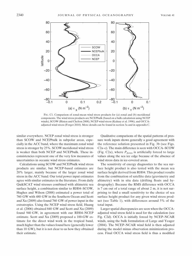
similar everywhere. NCEP zonal wind stress is stronger

than SCOW and NCEPbulk in subpolar areas, espe-

cially in the ACC band, where the maximum zonal wind

stress is stronger by 25%. SCOW meridional wind stress

is weaker than both NCEP and NCEPbulk. These in-

consistencies represent one of the very few measures of

uncertainties in oceanic wind stress estimates.

Calculations using SCOW and NCEPbulk wind stress

products are similar, but NCEP-based estimates are

20% larger, mainly because of the larger zonal wind

stress in the ACC band. Our total power input estimates

agree with similar estimates in the literature. From daily

QuikSCAT wind stresses combined with altimetric sea

surface height, a combination similar to RH04–SCOW,

Hughes and Wilson (2008) estimated a power total of

760 GW with 480 GW in the Southern Ocean and Scott

and Xu (2009) also found 760 GW of power input in the

extratropics. Using the NCEP wind stress field, Huang

et al. (2006) obtained 840 GW and Scott and Xu (2009)

found 940 GW, in agreement with our RH04–NCEP

estimate. Scott and Xu (2009) proposed a 100-GW es-

timate for the direct wind work in the tropical band,

much higher than the values found here (generally lower

than 10 GW), but it is not clear to us how they obtained

their estimate.

Qualitative comparisons of the spatial patterns of pres-

sure work inputs shows generally a good agreement with

the reference solution presented in Fig. 3b (see Figs.

C2a–c). The main difference is seen with OCCA–SCOW

(Fig. C2a), where Pdown is artificially forced to large

values along the sea ice edge because of the absence of

wind stress data in ice-covered areas.

The sensitivity of energy diagnostics to the sea sur-

face height product is also tested with the mean sea

surface height derived from RH04. This product results

from the combination of satellite data (gravimetry and

altimetry) with in situ data (drifting floats and hy-

drography). Because the RMS difference with OCCA

is 7 cm out of a total range of about 2 m, it is not sur-

prising to find a small sensitivity to the choice of sea

surface height product for any given wind stress prod-

uct (see Table 1), with differences around 5% of the

total input.

Larger spatial discrepancies are seen when the OCCA-

adjusted wind stress field is used for the calculation (see

Fig. C2d). OCCA is initially forced by NCEP–NCAR

winds, using the bulk formulation of Large and Yeager

(2004). The NCEP–NCAR wind field is then adjusted

during the model minus observation minimization pro-

cess. Final OCCA wind stress field is thus a modified

FIG. C1. Comparison of zonal-mean wind stress products for (a) zonal and (b) meridional

components. The wind stress products are NCEPbulk (based on a bulk calculation using NCEP

winds), SCOW (Risien and Chelton 2008), NCEP wind stress (Kalnay et al. 1996), and OCCA-

adjusted wind stress (Forget 2010). More details can be found in section 3a and in appendix C.


version of NCEPbulk. The OCCA wind stress field de-

parts importantly from NCEPbulk, having in particular

zonal wind stress within the ACC band increased by

50% (see Fig. C1). It is not surprising that the total power

input increases by 50% compared to OCCA–NCEPbulk

(Table 1).

Not only the total power input is increased by OCCA

wind adjustments, but the spatial pattern becomes also

more patchy, with the presence of strong negative–positive

pressure work spatial anomalies that are generally not

seen in the OCCA–NCEPbulk field (see Fig. 3b). These

wind adjustments are reshaping the pressure field at small

scale, possibly compensating for some missing physics

in the model. We suspect a misrepresentation of fi-

nescale current topography interaction at the OCCA

resolution as a principal source of bias counterbalanced

by wind adjustments. A more detailed study is still re-

quired to assess the detailed impact of OCCA wind ad-

justments, including a study of changes in the time-varying

contribution.

REFERENCES

Duhaut, T. H. A., and D. N. Straub, 2006: Wind stress dependence

on ocean surface velocity: Implications for mechanical energy

input to ocean circulation. J. Phys. Oceanogr., 36, 202–211.

Fofonoff, N. P., 1981: The Gulf Stream system. Evolution of Physical

Oceanography: Scientific Surveys in Honor of Henry Stommel,

B. A. Warren and C. Wunsch, Eds., MIT Press, 112–139.

Forget, G., 2010: Mapping ocean observations in a dynamical

framework: A 2004–06 ocean atlas. J. Phys. Oceanogr., 40,

1201–1221.

Gill, A. E., J. S. A. Green, and A. J. Simmons, 1974: Energy par-

tition in the large-scale ocean circulation and the production

of mid-ocean eddies. Deep-Sea Res. I, 21, 499–528.

Huang, R. X., W. Wang, and L. L. Liu, 2006: Decadal variability

of wind-energy input to the world ocean. Deep-Sea Res. II, 53,

31–41.

Hughes, C. W., and C. Wilson, 2008: Wind work on the geostrophic

ocean circulation: An observational study of the effect of

small scales in the wind stress. J. Geophys. Res., 113, C02016,

doi:10.1029/2007JC004371.

Kalnay, E., and Coauthors, 1996: The NCEP/NCAR 40-Year Re-

analysis Project. Bull. Amer. Meteor. Soc., 77, 437–471.

Large, W., and S. Yeager, 2004: Diurnal to decadal global forc-

ing for ocean and sea-ice models: The data sets and flux

climatologies. NCAR Tech. Note NCAR/TN-4601STR,

112 pp.

Marshall, J., A. Adcroft, C. Hill, L. Perelman, and C. Heisey, 1997:

A finite-volume, incompressible Navier-Stokes model for stud-

ies of the ocean on parallel computers. J. Geophys. Res., 102

(C3), 5753–5766.

Mazloff, M. R., P. Heimbach, and C. Wunsch, 2010: An eddy-

permitting Southern Ocean state estimate. J. Phys. Oceanogr.,

40, 880–899.

Orsi, A. H., T. Whitworth III, and W. J. Nowlin, 1995: On the

meridional extent and fronts of the Antarctic Circumpolar

Current. Deep-Sea Res. I, 42, 641–673.

Pedlosky, J., 1968: An overlooked aspect of the wind-driven oce-

anic circulation. J. Fluid Mech., 32, 809–821.

Rio, M.-H., and F. Hernandez, 2004: A mean dynamic topography

computed over the world ocean from altimetry, in situ mea-

surements, and a geoid model. J. Geophys. Res., 109, C12032,

doi:10.1029/2003JC002226.

FIG. C2. Time-mean contribution of Pdown estimated using dif-

ferent combinations of wind stress and SSH products. Two mean

SSH products are used: OCCA (Forget 2010) and RH04. Wind

stress products are as in Fig. 7.


Risien, C. M., and D. B. Chelton, 2008: A global climatology of sur-

face wind and wind stress fields from eight years of QuikSCAT

scatterometer data. J. Phys. Oceanogr., 38, 2379–2412.

Scott, R. B., and Y. Xu, 2009: An update on the wind power input to

the surface geostrophic flow of the world ocean. Deep-Sea Res.

I, 56, 295–304.

Stern, M. E., 1975: Ocean Circulation Physics. Academic Press, 246 pp.

Stommel, H., 1957: A survey of ocean current theory. Deep-Sea

Res. I, 4, 149–184.

von Storch, J.-S., H. Sasaki, and J. Marotzke, 2007: Wind-

generated power input to the deep ocean: An estimate using

a 1/10 general circulation model. J. Phys. Oceanogr., 37, 657–

672.

Wang, W., and R. X. Huang, 2004a: Wind energy input to the

Ekman layer. J. Phys. Oceanogr., 34, 1267–1275.

——, and ——, 2004b: Wind energy input to the surface waves.

J. Phys. Oceanogr., 34, 1276–1280.

Wunsch, C., 1998: The work done by the wind on the oceanic

general circulation. J. Phys. Oceanogr., 28, 2332–2340.

——, and R. Ferrari, 2004: Vertical mixing energy and the gen-

eral circulation of the oceans. Annu. Rev. Fluid Mech., 36,

281–314.


On the Patterns of Wind-Power Input to the Ocean...

Documents

Transcript of On the Patterns of Wind-Power Input to the Ocean...