ON THE PATH INTEGRAL FORMULATION AND THE

EVALUATION OF QUANTUM STATISTICAL AVERAGES

by

Arthur Manz

Thesis submitted in partial fulfillment of the requirements

for the degree of Master of Science

Department of Physics

Brock University, St. Catharines, Ontario

February 1979

© Arthur Manz 1979

To my parents, my cats and dogs

CONTENTS

SECTION PAGE

riCKilowxecigeiiienxs ....+...-..** + . . . . + . . . . * . . . . . . . . « * . . . . . 1 1 1

List of Figures . . . . . . . . . . . . . . . . . . . . . . . . . . . . . . . . iv

1. Introduction to the Path Integral Formulation ... 1

2^ Outline of the fork done in the Thesis . . . . . . . . . . 12

3. Mathematical Preliminaries •••••••••••.•••••••••• 16

4* Two Interacting One Dimensional Oscillators . . . . . 30

5. Lagrangian for an Anharmonic Crystal . . . . . . . . . . . . 89

6* The Method of Papadopolous •••••••••*••••••*••••• 44

?• Interacting Einstein Oscillators . . . . . . . . . . . . . . . . 58

8# Helmholtz Free Energy of an Anharmonic Crystal

9. The Debye-Waller Factor to 0(Aa)and 00^) . . . . . . . 84

10. Summary and Conclusions . . . . . . . . . . . . . . . . . . . . . . . . . 105

Appendices

Appendix 1 • •.••••••••••••••••••.•.••,••••••.•.• 108

Appendix 2 . . . . . . . . . . . . . . . . . . . . . . . . . . . . . . . . . . . . . . . . . . 112

Appendix 8 . . . . . . . . . . . . . . . . . . . . . . . . . . . . . . . . . . . . . . . . . . 122

References . . . . . . . . . . . . . . . . . . . . . . . . . . . . . . . . . . . . . . . . . . 124

i

Abstract

Four problems of physical interest have been solved

in this thesis using the path integral formalism.

Using the trigonometric expansion method of Burton

and de Borde (1955), we found the kernel for two interacting

one dimensional oscillators• The result is the same as

one would obtain using a normal coordinate transformation,

We next introduced the method of Papadopolous (1969),

which is a systematic perturbation type method specifically

geared to finding the partition function Z, or equivalently,

the Helmholtz free energy F, of a system of interacting

oscillators. We applied this method to the next three

problems considered•

First, by summing the perturbation expansion, we found

F for a system of N interacting Einstein oscillators^ The

result obtained is the same as the usual result obtained

by Shukla and Muller (1972) •

Next, we found F to 0(Xi)f where A is the usual Tan

Hove ordering parameter* The results obtained are the

same as those of Shukla and Oowley (1971), who have used

a diagrammatic procedure, and did the necessary sums in

Fourier space* We performed the work in temperature space•

Finally, slightly modifying the method of Papadopolous,

we found the finite temperature expressions for the Debye-

caller factor in Bravais lattices, to 0(AZ) and u(/K/ j,

ii

where K is the scattering vector* The high temperature

limit of the expressions obtained here, are in complete

agreement with the classical results of Maradudin and

Flinn (1963) .

Acknowledgements

The problems examined in this thesis were suggested

and supervised by Dr. R* C. Shukla» I would like to express

my gratitude to him for his constant encouragement and

personal help*

1 would like to express my gratitude to the Physics

Department, students as well as faculty, for putting up

with me*

1 would also like to thank OGS for their financial

support*

iv

List of Figures

Page

!• Hypothetical motion of a particle that is used

in developing the path integral . . . . . . . . . . . . . . . . . 22

2. All diagrams relating to the functional

differentiation in the derivation of the

Helmholtz free energy to 0(A¥) . . . . . . . . . . . . . . . . . . 83

3* Correspondence among the diagrams of the Debye-

Waller factor and the Helmholtz free energy of

oft*) • ••••• 104

1

1. Introduction to the Path Integral Formulation

In the more well known formulations of non-relativistic

quantum mechanics, one is interested in studying the

Hamiltonian of a system. This fact is evident when one

writes down the time-dependent Schroedinger equation;

where H is the Hamiltonian, 1P is the wave function, and

P\ is Planck's constant divided by S.Tf

There are many reasons for the development of the

Schroedinger formulation of quantum mechanics• The main

one is that for most cases, one looks for a one-to-one

correspondence bet¥vTeen the operators of quantum mechanics

and the classical quantities^ For example, one can

associate H aith the energy of the system.

However, one can formulate classical mechanics in

terms of an action principle, or as more commonly known,

Hamilton's principle, (Goldstein (1950)). .Vhen first

formulated, one was interested in the Lagrangian of the

system, and from the action principle, one obtained

Lagrange's eouations of motion. Later on, the Hamiltonian

was related to the Lagrangian via a canonical transformation.

In some ways the Lagrangian may be a more fundamental

function describing a system*

One may then ask the following questions* Is it

possible to formulate quantum mechanics in terms of the

Lagrangian, and if so, how can this be done?

2

The answer to the first question is yes. The second

question was partially answered by Dirac (1932) who laid

down the foundations of the path integral formulation of

quantum mechanics in his paper on the role of the

Lagrangian in quantum theory. Feynman (1948) proposed a

path integral formulation of quantum theory in terms of

the Lagrangian as suggested by Dirac (1932).

As is shown in chapter 4 of the book by Feynman and

Libbs (19o5), (from no* on known as FH), the Schroedinger

and path integral formulations are eauivalent in the sense

that the basic equations in either formulation can be

derived from the other, fhat makes the path integral

formulation worth studying separately is that it exhibits

certain interesting features that are not evident in the

Schroedinger formulation* vVe indicate some of these

features presently.

In the Schroedinger formulation, there are basically

two postulates. One of the oostulates involves the equation

of motion and the other involves the commutation relations

among ouantum mechanical operators, especially the

canonically conjugate operators. This latter postulate

is a consequence of the use of the Hamiltonian to describe

a system, and hence the need for canonically conjugate

operators. If instead, we use the Lagrangian to describe

a system, then we avoid the necessity o^ introducing

canonically conjugate variables, and hence we may be able

to drop the postulate of the commutation relations* Hence

3

we need only one postulate as Feynman used in his path

integral formulation.

It is appropriate now to give a brief sketch of what

arguments Feynman used in developing the path integral*

Suppose the Lagrangian of a system under consideration is

given by

L = irf- V(^p4) (1.2;

Here CL is the position coordinate of the system, (not

necessarily in one dimension), m is the mass, (not

necessarily a constant and could be a vector) , and V(%>i>A)

is the potential. Given the system starts at Q^lf^^J ,

we want to find the probability that it will arrive near

k£(fo» i) > >4* * Arguing that, in quantum mechanics,

probability is like intensity, one must find the sum of

the probability amplitudes of all possible paths from a

to b that the system can take, and then take the square

of its modulus to get the probability. Formally, one

can write this as

U.3)

where $fe#£J s probability amplitude of a path described by fM going from ct to b

Feynman postulated the following form for $[(l(i%

i>r<^)] = *«!> [jrStfWil ( 1*4)

4

"here sr^)] = f ' u ^ p i ) ^ (1*5)

anl the integral is evaluated along ad) . 3 is called

the action. In words, each path contributes eoualiy in

magnitude to K(fc,a) but differs in phase.

If we consider a one dimensional particle with a

potential V-V(o) that is well behaved, then the mathematical

prescription for calculating the sum over paths (or also

sometimes known as kernel) as given by Feynman (1948) is

6)

.vhere t. <£*. , A - ( ^ - ^ , f. -J. , f. • ?. .

and the integration is done over all possible values of Qj .

Feynman (1948) has also considered cases where the potential

is of a different form in the sense that V may depend on

f and 6 . Then the expression in Eq. (1.6) becomes

more complicated.

In defining the kernel, KOyO, in Eq. (1.3), one observes

that the function $[Q$] depends on the action st0l which is

a classical quantity. The £ makes the argument of the

exponential dimensionless, and brings in the nuantum

mechanical effects.

Intuitively, one can see that the oath integral

formulation has close ties ^ith classical mechanics. This

can be shown using the following arguments. If one

formulates the classical laws of physics using Hamilton!s

5

principle, the path taken by the system, that is, the so-

called classical path, will be the one that extremizes S[o(i)].

In the cases we consider, this extremum will be a minimum.

Observe that as we move away from the classical path, the

action will become larger, and because £ is small, $&$] will

oscillate wildly. Hence all contributions to the kernel

for paths that are not in the neighbourhood of the classical

path will cancel out, (Hunther and Kalotas (1977)). Thus

the classical path and the paths in the neighbourhood of

it will contribute most to the kernel*

In the Schroedinger formulation, the wave function of

a system associates a probability amplitude to the system

at a particular position and time. The wave function gives

a local description of the system. Furthermore, one must

impose certain restrictions on the wave function which may

be ad hoc or have a physically intuitive basis• fhile in

the path integral formulation, the kernel associates a

quantum mechanical amplitude to the motion of the system

as a function of space and time. This is more of a global

description. Also, the boundary conditions for the kernel

can be chosen a priori.

One of the more apoealing features of the path integral

formulation is that the arbitrary phase factor of the wave

function does not enter into the kernel because it is

already fixed.

Looking at the expression for the kernel given in Eq.

(1.6), one observes that one can perform the mathematical

6

manipulations as is done in classical mechanics. This is

also true for systems with other types of potentials,-

(Feynman (,1948)). Hence one avoids the troublesome task

of performing operator algebra. Since quantum mechanical

operators are still of importance because they are related

to physical quantities describing a system, one can use the

path integral formalism to define "matrix" elements of an

operator as was done by Feynman (1948), Davies (1963),

Cohen (1970), and Mandelstam and Yourgrau (1968).

Although the path integral formulation is conceptually

elegant, there is a major shortcoming which is expressed

in 3q. (1.6). First, one has to determine whether or not

Eq# (1.6) is well defined and second, one has to perform

the integrations given in Eq. (1.6).

In fact, to obtain the kernel, one must perform a

functional integral which is formally written as,

K(ka) * J MfM] exj, f| I LeflJ (1.7)

The expression given in Eq. (1.6) is similar in form to

the Riemann sum definition of the Riemann integral.

wiener (1923) developed, in connection with lirownian

motion, what is now called the wiener integral. The wiener

integral has a striking resemblance to the path integral

given in Eq. (1.6 J. There has been much theoretical work

done on the wiener integral and how it is related to the

path integral. This work is well covered in a review

7

article by Kovalfchik (1963). In fact, in developing an

expression for the density matix, one can use the .Viener

integral which is what will be done in section 3#

llore recently, much theoretical work has been done on

the study of Eq. (1.7). There are two points of concern.

One is that the expression given in Ea. (1.6) used in

defining the kernel given in Eq. (1.7) was developed on an

intuitive basis and so should be nut on a firm mathematical

basis. Second, the convergence of the integrals in 3q.

(1.6) must be handled carefully in a strict mathematical

sense. Fundamental work discussing these points include

Davison (1954), I to (1961), Keller and McLaughlin (1975),

De Witt (1972), Albeverio and Hoegh-Krohn (1976), and

Llizrahi (197?). The latter three references give a definition

of the path integral in Eq. (1.7) without recourse to the

limiting procedure as given in Eq. (1.6).

From a more practical viewpoint, considerable effort

has been put in to evaluate the path integral in EQ. (1.7).

Unfortunately, there are not too many cases that can be

done exactly, hence some effort is needed in finding good

approximations to the path integral.

A class of path integrals that can be done exactly are

the so-called Gaussian path integrals, that is, path integrals

with quadratic Lagrangians. Notable examples of physical

problems with quadratic Lagrangians include harmonic

oscillators, free particles, particles in a constant magnetic

8

field, and particles subject to a constant force.

Papadopolous (1975) has evaluated the general Gaussian

path integral, while examples of special cases can be

found in FH (Gh. 8).

Some of the work that has been done in evaluating

path integrals, either approximately or exactly, if possible,

will be presently given.

The expression in Eq. (1.6) can be used, but is

extremely tedious as is shown in FH (Ch. 3) for the free

particle, and in Devreese and Paoadopolous (1978), og. 123,

for the harmonic oscillator.

Davison (1954) developed the mathematics for evaluating

the path integral by expanding the paths in a complete set

of orthogonal functions• Davies (1957) and Glasser (1964)

expand the paths in a trigonometric series to evaluate

certain Gaussian path integrals. Burton and de Borde (1955)

use a different expansion in trigonometric series and

evaluate some Gaussian path integrals* This last method

will be discussed in section 3.

The so-called semiclassical or WKD expansion has been

explored* The method as described by Morette (1951) will

be discussed in section 3 for non-relativistic quantum

mechanics^ More recent work along these lines is that of

Gutzwiller (1967) and Levit and Smilansky (1977).

Much work has been done in expansion procedures also.

This involves the expansion of the part of the exponential

9

term of Eq. (1*7) that includes the potential or part of

the potential, in a power series and term-by-term evaluation.

Yaglom (1956) has followed this procedure in connection

with the evaluation of the partition function. For further

work on expansion formulae we refer to the work of

Papadopolous (1969), Goovaerts and Devreese (1972 a,b),

Siegel and Burke (1972), Goovaerts and Broeckx (1972),

Goovaerts, Dabenco, and Devreese (1973), and Maheshwa'ri

(1975).

In some cases it may not be possible to get a good

approximation to the path integral. In those cases then,

one may be able to get some bounds on what it should be.

Specifically, these bounds are in terms of some physical

quantity describing a system. Feynman^(FH (Oh. 11))

developed a generalized variational method In which he

obtained an upper bound for the Helmholtz free energy of

a system.

There are other methods for evaluating the path integral

but they will not be indicated here.

The Feynman formulation, and hence the use of the path

integral and wiener integral^ has been applied to solve or

at least partially solve some important problems of physics*

The areas of physics where the path integral has been

applied include cuantum, statistical, and solid state

physics.

One of the most notable successes of the path integral

formulation has been in the determination of certain

properties of the polaron as described by Frohlich (1954),

such as the effective mass* Some of the work done on the

polaron include Feynman (1955), Osaka (1959), Schultz (1960),

Feynman, Hellwarth, Iddings, and Platzman (1962), and

Thornber and Feynman (1970).

Feynman (1955) used the variational method, as noted

above, in determining the effective mass of the polaron^

This variational method has recently been applied by Celman

and Spruch (1969) to problems in which the Hamiltonian of

the system being studied has a term containing angular

momentum.

Pechukas (1969) has used the path integral to derive

the semiclassical theory of potential scattering*

Papadopolous (1971) has applied the path integral to

the problem of a harmonically bound charge in a uniform

magnetic field, from which he evaluated the partition

function and density of states*

Lam (1966), Maheshwari and Sharma (1978), and Seshadri

and Mathews (1975) have done some work on approximating

the kernel of a one dimensional anharmonic oscillator with

potential V(*) = <*** + *>***•

Khandekar and Lawande (1972) and Goovaerts (1975) have

applied the path integral formulation to a three body

problem considered by Calogero (1969)*

There are many more applications of the path integral

11

formulation, some of which are of far greater importance

than those mentioned. Many of these applications along

with some of the theory of path integrals and Wiener Integrals

is given in the review articles of Gelffand and Yaglom

(1960), Brush (1961), Barbashov and Blokhintsev (1972),

and rfiegel (1975;- The standard text on path integrals is

FH which gives the path integral formulation as developed

by Feynman along with many applications including Feynman1s

work on quantum electrodynamics. More recently, the book

edited by Devreese and Papadopolous (1978) gives some of

the other developments of the path integral formulation and

the present status of the path Integral.

Before we end this introduction to the path integral,

there are three points which should be noted.

First, Davies (1968) and Garrod (1966) have develooed

the path integral using the Hamiltonian. They showed that

their path integral is the same as that using the Lagrangian.

Second, Eandelstam and Yourgrau (1968) have related

Schwingerfs variational principle to the Feynman path

integral formulation.

Finally, work has been done in evaluating path integrals

in general curvilinear coordinate systems other than the

usual cartesian system. ?,Iost of the work has been done in

polar or spherical coordinates; for example see (Edwards

and Gulyaev (1964), Arthurs (1969), Peak and Inomata (1969),

and Arthurs (1970))•

2. Outline of the fork done in the Thesis

Four problems of physical interest will be tackled

using the path integral.

As can be found in many standard textbooks on solid

state physics (Kittel, for example), a model that is

freauently used in describing the dispersion forces of

condensed matter is a system of coupled oscillators. In

section 4, we use the expansion in trigonometric functions

as discussed in section 3 to evaluate the path integral

for two interacting one dimensional oscillators without

using a normal coordinate transformation. This problem

has already been solved using the normal coordinate

transformation as is shown in FH (Gh. 8).

The partition function, or equivalently, the Helmholtz

free energy, F, is an extremely useful ouantity in describing

systems which are in thermodynamic eouilibrium. However,

for a system of interacting oscillators, such as an

anharmonic crystal, it is difficult to find an exact

expression for F# Hence one must develop approximation

methods to get F, one of which is a perturbation type

expansion. In section 6, ve derive the method of

Papadopolous (1969). This is a perturbation method using

the path integral and functional differentiation. TJsing

this, we develop a systematic method of obtaining the usual

perturbation expansion of the partition function for a

system of interacting oscillators* This method is

specifically geared for a system of interacting oscillators

and will be applied to the next three problems discussed.

In section 7, we find the free energy of N interacting

one dimensional Einstein oscillators. This oroblem has

already been solved in the same vein by Shukla and Muller

(1971) using a Green function method and again by Shukla

and Muller (1972) using a diagrammatic procedure. In

studying this problem, one is looking at the simplest

problem which exhibits certain features that occur in more

realistic models. To simplify greatly the calculations

needed, one transforms the problem to wave vector space.

In this space, one can use the symmetry of the system to

apply periodic boundary conditions and develop the dispersion

relationship. Also, when one is doing the perturbation

expansion, the expansion cannot be cut off anywhere to give

correct results because the interaction term is as strong

as the harmonic part of the potential. Hence, one must

sum the series to infinity.

The next two oroblems studied have to do with the

anharmonic crystal. The interaction or anharmonic parts

which are expanded out, are generally much smaller than the

harmonic oarts in their contribution to certain properties

of a crystal, but are still necessary to describe the

properties of a crystal such as thermal expansion, specific

heat, etc. Perturbation theory is a standard method used

in studying^ theoretically, the properties of a crystal.

14

In section 8, we find the free energy of an anharmonic

crystal, or system of anharmonic oscillators, as described

in section 5, to 0(\H) , where A is the usual Van Hove

ordering parameter* This is the second lowest order of

perturbation that gives a non-trivial contribution to the

free energy. It has been found that the lowest order of

perturbation, that is 0(Ay f is inadequate in describing

the temperature dependence of the heat capacity of certain

materials at high temperatures, and~hence, one must include

the next order of perturbation to account for some of the

discrepancy. Shukla and Cowley (1971) have done this

calculation by using a diagrammatic procedure, and evaluating

the necessary sums in Fourier space, rfe will perform the

calculations in temperature space* These calculations have

been done in temperature space to 0(XZ) } (Papadopolous (1969),

and Barron and Klein (1974)), but to our knowledge have not

been done to 0(A*) # The results we obtain are equivalent

to those of Shukla and Cowley. As a further sidelight, we

will indicate how one can draw Feynman diagrams from the

expressions we derive.

The decrease in intensity of x-rays scattered from a

crystal occurs because of the thermal vibration of the atoms

of the crystal about their lattice sites, and is accounted

for, in theory, by using the Debye-Waller factor. In section

9, we determine the Debye-Waller factor for a monatomic

Bravais lattice, which is a special case of the system

15

described in section 5 to 0(f) and 0(/K/¥J y where K is

the scattering vector. *Ve do the calculation to Off) because

this is the lowest order of perturbation that gives a non-

trivial contribution to the Debye-Waller factor. The reason

for doing the calculation to O(lK)1) is that if one were to

write out the full formal expression for the Debye-tfaller

factor, one "would find that the lowest order term is

proportional to IW and the next lowest order term is

proportional to lKl¥ f but both terms are of 0(f) in

anharmonicIty. We then take the high temperature limit to

show that our results coincide with those of Maradudin and

Flinn (1968). Current numerical techniques make the

calculation of the terms of the Debye-Waller factor extremely

time consumingf even for the high temperature limit. However,

the finite temperature results are of some interest in

investigating the temperature dependence beyond the leading

temperature terms derived in the classical procedure of

Maradudin and Flinn (1968).

In section 10, we summarize our findings and make our

conclusions•

3. Mathematical Preliminaries

In this section, we present a mathematical formulation

of the path integral starting from the time dependent

Schroedinger equation and Its general solution. We then

describe two methods for evaluating the path Integral;

(a) the semiclassical or #KB expansion of Morette (1951)

for non-relativistic quantum mechanics, and (b) the

expansion in trigonometric series as given by Burton and

de Borde (1955). The trigonometric expansion method will

be used in section 4 to solve the problem of two interacting

one dimensional oscillators. The method of yorette will

be used in section 6 in connection with the study of a

system of N interacting Einstein oscillators (Sec. 7), and

the anharmonic crystal (Sec. 8, 9). Finally, we show how

the density matrix can be written in terms of a path

(Wiener) integral. The density matrix, and hence the

partition function, Z, or equivalently, the Helmholtz free

energy, F, will be employed in sections 7 and 8.

(A) The Path Integral

The time dependent Schroedinger equation is

U W =il sL£ (1.1) H

where the symbols are defined in section 1. Suppose the

Hamiltonian is given by

H=-Lf>* + Vfy) 13.1)

where b,CL are the usual momentum and position operators,

respectively, (not necessarily one dimensional), m is the

mass which is appropriate for the system considered, and

Vl^J is the potential which depends on position only.

The general solution of Eq* (1.1) is then separable

in the sense that It can be written as the product of two

functions, one depending on time and the other on position.

It then remains to find the energy eigenvalues and

eigenstates of the associated time-independent Schroedinger

equation. Let the stationary eigenstates be (pf(?j and the

associated energy levels be E « As is well known, the

set i^Jf)j forms a complete, orthonormal set^

Using the notation of section 1, and following the

procedure of Schiff (1968), the wave function x(C^TJ of the

system under consideration can be expanded in terms of the

energy eigenstates to give

^(a) = (^"U " T- Qs (W 4>B (fa) (3-2)

The wave function xf^/ywhere ty ^ta is given by

Let

K(ka) -o

(3.4)

Then, Eq. (3.3) becomes

f

W ) = J KCIo.a) 1PU) dj, (3.5)

K(h}Gj is often called the kernel, propagator, or Hreen

function.

Essentially, Eq# (3*5) is an integrated version of

the Schroedinger equation, for given the wave function at

some point in space and time, and the kernel, one can find

the wave function at later times.

We note the following three important properties of

the kernel*

First, K (*>,*) s K ^ > f c i V O (3.6)

The kernel Is a function of the difference in time*

SeCOnd' ti»J(k*)* ^.\(f)^(jJ'S(p-f.) (3.7)

where in taking the limit i^ia $ it is understood that

one approaches {^ from values greater than 4^ * The last

equality is just the closure property, with SOjbrfr) denoting

the usual Dirac delta function.

Third, suppose that C=((?04) s a n intermediate point

such that 4<^c<^i * Then, by Sq. (3.5),

19

my) - J K(KC) wed dfc

whence f ffc) = J V ? a [ JVj f t / < M K(c}a)] 9(a)

Comparison of the above equation with Eq# (3.5) yields

K(fc,a) = Ufc K(h,c) KCCA) (3.8)

One can proceed along the same~ lines as above to

obtain the following;

where ^t> c >"*>^cl>^a

In what is to follow, we shall restrict ourselves to

one dimensional cases* The extension to higher dimensions

is straightforward and follows along much the same lines

as the extension of the Riemann integral to higher dimensions.

Now we will show, in a sketchy manner, how to express

Kffcya) in the form of the path integral.

It is well known that the energy eigenfunctions of a

free particle of mass m are given by ^Blp~^f>ukp , and

the associated energy levels are g >, &zk* , where k is

the wave number* The energy levels are not discrete, but

instead form a continuum, whence 21 —^ — J dk E "^

For \ ^ \ , Eq* (3.4) becomes

The Lagrangian of the free oarticle is given by

L = j[m % • Solving the corresponding Euler-Iagrange

equation subject to ($'^*)~%<L > and fy^v ~ %l> > and

substituting this into the action integral, #e find that

the action S , is given by

SsS(k,a) . f \ ^ = ffi (3£l^ (3.11)

Noting Eq. (8.11), we observe that Eq* (3.10) is

MJ--lApsl* "M5^ (3-12)

He note that the form of KCb^o.) given in Eq* (3.12) is

similar in form to the kernel given In EQ. (1.6)*

Suppose now that instead of a free particle, we

consider a particle whose Lagrangian is given by

L - ^ r ^ (3-is)

where V is the potential, depending only on the position

of the narticle*

Without getting into the mathematical details, we

will derive an expression for the kernel of this particle

which is similar to Eq. (3.12).

Suppose H ? ^<i • Subdivide the interval F «>" J into

N subintervals, the j such interval having length £ >0 .

J

Put •£, = "ca + 21 G» t with -^=^4 and iN

= i>* With each

-t , we associate the position coordinate Q.. . Let j=(olX

Noting Eq. (3.9),

K M = jdf)-'SclfN., K(KN-l)"K(j+Lj)-KO><0 (3.i4)

If the 6. are small and Via/ is a fairly smooth

function, V(j)^Y(fj) for * j ^ **(*/• The Lagrangian of the

particle in the interval ^j^*\/+) is then approximately

given by L ** ^tn 6 - V(fJ s l~., .

If one wvere to picture the approximate motion of the

particle from a to b , one could conceive of the particle

as moving like a free particle In the time Intervals "d- Lj

while the points ^fjjjt^ a c t a s scattering centres of the

particle that change its energy by V'fj'-V(frX (see fig. 1).

Hence, •

„ AJt\ JS<J+>'J> (3.15)

where AJt, - F *? j , arid 5(/+/,j)=J i-jc/4 , with J satisfying fc^ J

the corresponding Euler-Lagrange equation for -Ls^^ij^.

Note that 4EU)-€ J > k2k%2m(E^)/(iJl and the eigenenergies

form a continuum just as in the free particle case*

22

Figure 1: Hypothetical motion of a particle, with its

Lagrangian given by Eq^ (3.13), from Q-fa^a) to

b« fafc/k'* The scattering centres are the

dots and the straight lines indicate the free

particle motion between scattering centres*

FIG. I

22a

N-l

VI

t -

— -*

V V i " fj

/ /

/

t o l "

/

/

J L J L

qa q. VI qN-| qb

Further ^ A , , ) ^ ' ^ because t3^i<^, . Substitution of

Sq. (3.15) into Eq. (3.14) yields

K(M * J & ... I^E | e*J- H f= W /

If we let r*ax€-*0*, or if all the 6. are eaual^ we let A) ?+*> j J J i

one observes that the approximation becomes better. Hence

we expect

K(b,«) « "" J $1 - i lp -jr ext.Htstj.l.j)] (3.16) nK y max€^0^J Ai J AN-» ^W

r(<j=0 J J J

J J

This is the same as the expression given in Ecu (1.6)

(B) Methods of Evaluation

(a) 3emiclassical or WK3 Expansion Method*

Let us first consider the method of the semiclassical

or 1KB expansion as given by Morette (1951). ;/e consider

the case for non-relativistic quantum mechanics instead

of for relativistic quantum mechanics as was done by Korette.

is given by ^ - ^ U ^ f i The action

Let xcW be the function which minimizes StaJ f that is,

zt(i) is the classical path* Let Q(4)~ xcd)+/u(4) . Hence^

Expanding S about xcU) in a Taylor series, one has

sl}l - SU1 * i, fsH'jfS'JUt- (3.i7)

where 8 represents the variation of S and xc=~xc(i) is

defined by S$fxe3 = 0.

As an approximation to S , we drop all terms higher

than second order in the expansion of Eq# (3*17).

P^ SA = SfxJ +±S*SL*J (3.18)

where s ^ w . ^ ^ff^] f^>^ +

and ZL is the sum over the components of Q,.

The kernel for the action S^ , is then given by

K , M « / j ^ e * 4 = ymtNhrtfr&H&Ml (3.19)

We will give an intuitive argument for what follows

next, but the following can be done rigorously, (Kovalfchik

(1953)).

•Ve have written oU)^xc(i)f^(i) . Now, Xcli) is a fixed

path and hence cannot be varied. It follows that m(i) is

the path to be varied with mrliJ^^H'^-O m Essentially what

we have done is to perform a linear transformation* Further,

since S[xcJ is independent of Attt) , we can factor exb{4-5feci]

out of Eq# (3.19) as though it was a constant* It follows

that y(ti)*0

KA M = e***3 J M7M1 [i i W ? (3.20)

The above path integral is not necessarily zero, but just

states that we must evaluate the oath integral for all paths

starting and ending at the same space coordinate, namely 0.

One can determine the path integral of Eq* (3*20)

using the methods of Lforette, and is given by

I. mym^U^shjj.j^ ' | s w y (3.21)

The above method Is exact for Gaussian path integrals

because $nS[xcJ^0 for n=3,4,.*. . In fact, the second

factor on the right hand side of Eq. (3*20), for this case,

is independent of oaand o^, and depends only on iA and #

(b) Trigonometric Expansion Method.

He now wish to discuss the method of expanding the

paths in a trigonometric series as was done by Burton and

de Borde (1955)* We will again just discuss the one

dimensional case, but these results can be extended If so

desired. Instead of using the general time interval r , j>J>

we will use ft T] m There is no loss of generality for the

cases we consider^ since the kernel depends only on the

length of the time interval^ as is observed in Eq. (8*6)*

To evaluate the action integral, we exoand the velocity

term arising in L as follows;

^-(^ga^Jd (3. 2 2,

where ^fz) = / $ ^m(^-{2tos>(nwit)>n>l , and the tf» are

independent of t. Plainly, \%(^)f form a complete,

orthonormal set of functions on lO^T] as they are the

functions used in Fourier cosine series expansions*

To find <LU) , we integrate the expression for w ,

noting that a(0)s«Al and <^T) = | t • Integration of Eq. (3.22)

H^fa+^h^Ml^ Further, %(T) -^ = £k-f<t « ($-)** J

<V>) i t Q a = *»» ^ _„ ^ ( 3 . 2 4 ) 0 STiKT

The beauty of the method can be seen from the above

expansions. One observes that the expansion coefficients

[a*] characterize the path. Intuitively, at least, if one

integrates over the Qn > one would be summing over all

paths. The mathematical details involved are not trivial,

and will not be given here. However, if we substitute " o.

(3.22), Eq. (3.23), and Eq. (3.24) in L, and then find the

action integral in terms of the a„ , the kernel, K(h}a), is

then given by

The integrals are over all possible values of the dH , ft*(,

Oft being fixed by Eq. (3.24). The factors Z7 and /_!22__-)*

can be obtained by comparison with the result for a free

particle which can be done by first orinciples, (FH (Ch. 3)).

The other kernel needed in this thesis is that of an

harmonic oscillator, the derivation of which will be given

in section 4.

(0) Density Matrix

We now introduce the density matrix which is very

useful in statistical physics, rfe then show how one can

write the density matrix as a path (wiener) Integral

following the method given In FH (CJh. 10).

Are know? from statistical physics, that for a system

in equilibrium and in thermal contact with a heat reservoir,

the partition function Z, or equivalently, the Helmholtz

free energy F? is all one needs to deduce the average

properties of that system.

The partition function is defined as follows;

Z = H e ^ £ r 13.26) v

where E r energy of state r of the system,

A= -J— , kB 2 Boltzmannfs constant,

B T s absolute temperature,

and JL is the sum. over all possible states of the system. r

The Helmholtz free energy Is given by

F= ^k8T Ai2 (3.2?)

In what is to follow, the system can be described

by the Hamiltonian given in 3q. (3.1). Je can obtain

28

the following results for other types of potentials, but

the arguments needed must be changed*

If state r is defined by the normalized wave function

fy (q) , the probability of finding the system in state r

"near" CL , that is, in the region 'ftj£*0J» is given by

Pr(f) df = £ e ^ tfty 4rty) ctfr (3.28) Here, we have also assumed that the system is in

eouilibrium, and is in contact with_a heat reservoir at

temperature "T . Summing over all possible states, the

probability of observing the system "near11 O is given by

P(f) dt-Z. Pr(f)^ - ± z. *& tffy Utfdfr <3 •29 > If we are instead interested .in a quantity u , say,

where & is some property of the system, then

B =^Z.<B>re-v4E"-^r/^)5<|)<(^)^e^E'- 0.30,

The bar denotes thermal average, and \ /r denotes quantum

mechanical average with respect to state r@

If we know the quantity

e (f <£> = T. britf &(f) £~^r (3.31)

we can evaluate 3 , remembering that if B-B(G) f it

acts on <f>r(fly. O is called the density matrix.

We note the following;

2 = [p^f^i s Tr p ; (Tr = trace) (3.32)

PCJ) - ^ e ( ? * r (3*33)

8 = J-Tr (8p) (3*34)

Comparison of Sq. (3.31) with 3q. (3.4) yields,

formally at least,

i

- J*/rr«&3 «/> [- j f e "^ + V^)]] (3-35,

The above integral is what is more commonly associated

with the Wiener integral (Oel1fand and Yaglom (I960)).

Yaglom (1956) demonstrates how one can derive Eq. (3.35)

in a more rigorous fashion.

4. Two Interacting One Dimensional Oscillators

In this section, we use the method of expansion in

a trigonometric series, as explained in section 3, to find

the kernel of two interacting one dimensional oscillators.

Let the independent position coordinates of the

oscillators be given by X, and x2 . We use a subscript 1

to label the various quantities relevant to describe one

oscillator and a subscript 2 for the other oscillator.

Observe that two sets of coefficients will be needed

for the trigonometric series, one for each Independent

coordinate. Thus, instead of integrating over one set of

coefficients, we must now integrate over two sets.

The Lagrangian of the system can be written in the

folloT#Ing form;

where ^j^Jmj (^^^/xfh J-M • Let K u * yjf^mx U)10

Suppose the boundary conditions of the system are the

following;

XJ(0)^QJ , * y f D = ^ i j = / > 2 (4.2)

As given in Eq. (3 .22) , l e t

£ (i) = (Mk)* H C*, k (r) ; r]>2 (4 .3)

where, now, the Cni are the expansion coefficients.

According to 3q. (3.24),

°J m LL_ (t,-«i) ; j=/,2 (4.4)

and to Eq. (3.23J,

Substituting the above expressions into H and L, ,

and doing the appropriate integrations, we have, (Burton

and de Borde (1955), Brush (1961)), for 1=1,3. ,

5 )

J. I V -^[^-iW+to+tf +e0

T

r»s/I jnzTf:i/ J KnTr/\-hT ' J -J J J ( 4 ' 6)

Finally, for » = '»* ,

T

>TY-

where, in obtaining Eq. (4.7), we have used

U.7)

r> + /-r-.a.

*7T o T

rvVMe

Us ing Eqs» ( 4 . 6 ) and ( 4 * 7 ) , t h e a c t i o n i s g i v e n by

2 L j* 3

Substituting Eq* t4.8) into Eq. (3.25), the kernel

is given by

Kcu. -T) - (^THi^ntmdw (4

Since the coefficients Cwi and cn^ do not mix In

each term of the expression in Eq. (4.8J, we can separate

Eo. (4.9) into a product of double integrals.

Me Introduce the following notation. Let

Collecting all terms containing Ch| In Eq. (4.8) yields

Jw - * °nl I C m — — • — — — CM|

t y j

(4*10)

mi

Integrating over Cnl , #e find

Collecting all terms in the exponent of the exponential

containing Cn2 in Eq. (4.11), and 3q. (4.8) gives

(4.11)

I»= I

Integration over Cm2 yields a.

--o JT * & ,

c y

(4.12J

Employing Eqs. (4.11), (4.12;, and making use of the

following identities;

(i) Tr(^,VMa - h) = (/- ^qfj[l- T^FV

where c * = 1 [ ((»?+«>?) ± J C^-co^ + W } (4.13)

34

the kernel (Eq. (4.9)) can be expressed as

« ^¥?i zin(u>jT)'

T:

14)

r 6

where Q = 'i^Qh

Q W *»' C ,2 - vk, O

lit'

The above expression for Q w can be simplified to

+ [A; (V-^V^%3^»j

where

a. ^rr^ r , />*-«?<>, t , ( - / n

B* ^ ^ U ^ I - ^ A ^ J KT

35

ha7Ta/ I h*W

Dn -

Using the following identities,

(iii) T - J _ _ = £ [-L - JL Coi(^) - f 7 / ** /s »°+

(iv) f (-/)" =J_ o . ir c s c f r t ; + 2 ?? l W e * e r

and the expression for Qn , we find the following complicated

form for Q ,

•*• *»a ( « > 0 (*>/ " ^ > / +^>"+ 3 " > ^

fJll f-ILL - "^ /, -r) id ?

"ILL [ H i - J£ cot (a, T)-g II

~ r - , w(&, k (^ti-Ojfcol

Hi-cofco,i-h Sto^a)")

- 7 7 * C 7TX

CSC

+ fm, (afi-k*) (co^-hw1') ^ / m ^ (a, + b, ba ) (A> z (ui*+ cv*)

' ^ ( i ^T 2 ~ 2^rCoi ^ r ; " T ~ 7

+ 7 T 77a

&L a-ra ^ T 1 ( Zoo.T

-ELcoHu>„T) -J?]] 2to_T *> J 1

* f TT* r TT3 77* / T ) 7T-2 ?

Finally, substituting the above expression for Q

into Eq. (4.14;, and considerable manipulation we find

the kernel to be

*u y

where a.

V to*-or1/ \ Ui*-tu*/

In fact, the expression in Eq. (4.15) is the product of

kernels of the two harmonic oscillators with frequencies

u)± and OL , respectively* These frequencies have

been modified from the frequencies tv% and u)x because of

the interaction.

The author has tried to extend this path integral

method to the case of a linear chain of N interacting

oscillators, but the expressions soon became excessively

complicated, hence the work was discontinued.

If we let K,a =0 , Eq. (4.1) reduces to the case

of two non-interacting oscillators. If oo*Zu)z , then from

3q. (4*13), we have «o+-u)t , and u)_~t»A. In this case then,

Eq. (4.15) reduces to

i kVik Sln(toj) / ' ^SlMTfc^)

which is nothing but the product of the kernels of the

individual oscillators of frequencies &>, and coz ,

respectively.

For dispersion forces in condensed matter, as is given

in Kittel (1976), pg. 78, we set

K'3 R 3

where e is the charge of each oscillator, and R is the

interparticle separation. The zero point energy is then

where CV+ and w^ are given in Eq. (4.13). Expanding U)^

and u;. for small interaction, we get the interaction

energy, which varies inversely as the sixth power of R.

5. Lagrangian for an inharmonic Crystal

In this section, we set up the Lagrangian for an

anharmonic crystal, that is, a system of three dimensional

interacting anharmonic oscillators. The basic procedure

followed is that given by Born and Huang (1954). We

assume that we are dealing with a perfect crystal that

has N cells. tfe further assume that periodic boundary

conditions hold, and that the usual adiabatic or Born-

Oppenheimer approximation is valid.

The Hamiltonian for the crystal is given by

M = T + $ ( 5 . i )

where "J" = kinetic energy

Here Jt s cell index,

K - index for different atoms in each cell,

rf. a x,y,z components,

Mg H mass of K atom, and

f£(v)s *C component of the momentum of the K

atom in cell Jt .

<p H potential energy

where %( ) = the equilibrium position of atom H in cell /

= x(£) + *(#)

Here, t fi) *i,(*. + i a % + i 5 % , £M = l<A + Ki^+ K,% , and

l^ij^2j^3j is the set of fundamental lattice translation

vectors• \JL\ > 2 > 3 J is a set of integers, and fK^K- W3J

is a set of non-integer numbers such that O ^ K,, H > M 3 I

^M tf) s "t^le displacement °^ Qtom K in cell Jt from its equilibrium position*

Assuming that the ^(gj are small, we can expand (g

in a Taylor series about its equilibrium position, whence

£K*

3l S TTw' t^(Jj5- £»)^(.i)«*'($)«*'(** JL'K'd'

whe re d) = 0 j - constant, and hence can be neglected -6 jj_0 in the following work,

t(i) = = c, z*=o

since there is no net force on any atom, I or K , in the

like,

d«<(i)K($ f etc*

tt=0

Substitution of the above expressions for T and $

into Eq. (5.1) yields

H = H0 + HA (5.2;

where

H = Zl P ^K) +-LZ. &Ju')uJ*)iu-(£)''aa

" " *M* ;<*v

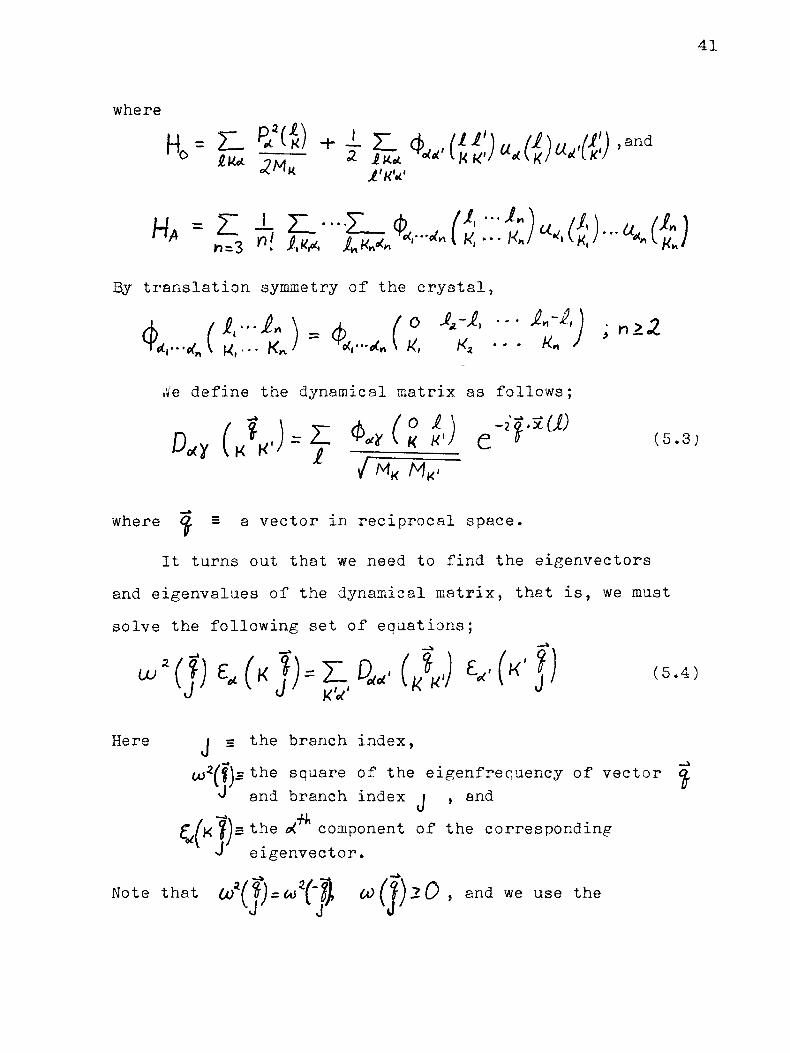
H*= £, i fc-fc.^ft""-iK^)-^(iJ By translation symmetry of the crystal,

le define the dynamical matrix as follows;

z D-y (K?K'J = ^ ^ ^ ^ e"'* (5-3)

where 4 = a vector in reciprocal space*

It turns out that we need to find the eigenvectors

and eigenvalues of the dynamical matrix, that is, we must

solve the following set of equations;

KW

Here j s the branch index,

U)*(f)s the square of the eigenfrequency of vector o J and branch index « , and

^f-B the component of the corresponding

eigenvector*

Note that (*)*(%) = (***("$, (A)(i)lQ , and we use the

42

convention t* (K ?) = £^ ( K ~|)

We now introduce the normal coordinate transformations.

These are given by

Note that r(t).P($ and Q*(J)"= 0("jfj •

Then, substituting Eq* (5.5; into Eq* (5*2), and

performing the usual operations, (Born and Huang (1954)),

we get the following;

f J

H,--Z ^ - ^ ^ J » - 4 J " ) ^ ^ - W I D (5.7)

where

I 11 ecu J*/

and f 1, if <7=tO or Is a vector of reciprocal

A(o)= ] lattice,

0, otherwise•

To apply the path integral formulation to the problems

to be considered, we will need the Lagrangian of the system*

Hamilton fs equations yield A / f 1 « ^ H _ D/~?1 •

Here, we note that for every vector o in the sum over Q, ,

there is a corresponding vector -"<£ .

The canonical relation between the Lagrangian and

Hamiltonian yields

= L 0 - U ^5-8>

where ^ = i JL [fi(/JQ^J-^Q(j)^-J) J , V

LA = HI

We introduce the symbol A cLlr , noting that -~\~ ~9rW

Then, we write Q(%r)=Q(^ Q^ Q f ?j = Q ^ ,and ^(|) = ^ = ^

An important property to note is that V \AD**<J **'

is completely symmetric in its arguments A|,...jA*

Thus, L^ is invariant under permutations of Pv J «

6. The Method of Papadopolous

tfe now introduce the method of Papadopolous (1969),

which is used for evaluating the partition function z, and

hence the Helmholtz free energy F, of an anharmonic crystal•

We have to change the derivation slightly from that of

Papadopolous, but the basic ideas used are the same*

The Lagrangian of an anharmonic crystal is given by,

Eq. (5.8),

L A . £ ZLV"(X„..A)QV-QV

(5.1) + 00

»«3 VOU

For this Lagrangianf the density matrix of the system

is given by, Eq* 13*35),

Q(o>£ (6.?)

where Jft [Q(s)}-WSt^(^ ®n& zi > a n d fa a r e t h e boundary

coordinates* x# and hence, Q is a vector with the

same number of components as there are different values

of Ar .

Jj'rom fiq. (3.32; ,

z= f^Xe^S) (6.3)

where d%t-Tfo(f,^ and the i n t e g r a l extends over a l l possible

values of A

45

As it stands, the path integral in Eq# (6#2) is not

known to have a neat closed form solution* Hence, to get

some meaningful results, an expansion (perturbation)

procedure is used on the term exfe f - y L //q

Formally expanding exb £-J L a n ? we obtain the o

following;

o

A^A^A,, 0

AA2A3 A¥AjA^

0 0 7

- . . . (6.4)

Substituting Eq# (6*4) into 3q* (6*2;, and then

substituting this into Eq# (6*8) yields a linear combination

of terms, a typical term of which that has to be evaluated%

neglecting its coefficient, is of the form

where fl^gfc,] = fgfc)] exj, [-!£ fh&&"#&]? ( 6 ' 5 >

Js IQl^u represents the measure used for the "averaging*1

process. Here, we note that it is of the same form as the

Uhlenbeck-Ornstein measure, (Maheshwari (1975)). Further,

we expect that the convergence behaviour of the above

expansion will be the same as that of ordinary perturbation

theory since we are developing the perturbation expansion

via this method.

From the Gaussian character of the measure, it follows

\f...y* with an odd number of indices

will contribute nothing to the expansion. That this is so

will be sketched out in appendix 1. The way to evaluate

the contributions from those terms with an even number

of indices will become clear later on, and will be evaluated

in later sections, (see sees* 7 and 8).

He note an important property of the J i.., * • As

can be observed from Eq. (6.5), it follows that any

permutation of the indices for a given variable Sc , say,

will leave X** .\* unchanged. This will be important in

simplifying the various terms of the expansion for Z.

Combining the above results, we have

(0

X [Zl V Y U * A J W \ ^ V T ; , A ; J M + - " ]-••• (5.7)

where

-j (6.8)

g the partition function for a system of

non-interacting harmonic oscillators^

Instead of evaluating the separate terms of Eq. (6.7)

using Eq. (6.5), we can more easily generate these terms

employing a "source term"/^(Tarski ("1967)). Although we

have followed Papadopolous (1969) and Tarski (1967) in the

work presented in this thesis, the idea of introducing a

"source term11 in quantum statistical physics problems was

Introduced as early as 1951 by J. Schwinger.

We will show a little later in this section that

obtaining Z is formally equivalent to the knowledge of

some generating functional. The procedure then is to — (n)

evaluate the integrals L,. m . arising in Eq. (6.7), and A, *

explicitly given by Eq. (6.5j^by functional differentiation

of the following generating functional, viz*,

A G = jVj r#rgfc)W ^ lJsWQ4*>} (8.9)

Then Eq. (6.5J can be expressed in the form

At Am j A! Ap C ° £ 0

s s s ) SJ^(s)S^k) "si^J

?«/>fffH*)<$ (6.10)

J=0

48

with the help of r yj($)Q(s)cl$ ^ . > fj(s)Q(s)ds

OTs) e J '

Since it is possible to perform the functional

integrations over IQ^x^S > then the various functional

differentiations, and finally the integrals over £scj f

(Papadopolous (1969;), Eq. (6.10) can be expressed in the

following form;

_ G

J=0

(6.11)

What remains left is to evaluate Eq. (6.9; which first

requires the evaluation of the following path integral;

=?w® f-# l&w^+*%c Wj< 6. where in obtaining Eq. (6.12), we have used Eq. (6.6).

He suppose the Ar comoonent of ji can be written as

fx-Xx^iMA ; JfAi/%A a r e r e a l # i^ince &(s)-Qjs), then § - f .

Since Eq. (6.12) is a Gaussian path integral, we use

the semiclassical or WKB method outlined in section 3 to

evaluate Eq.. (6.12) T Hence, we have the following;

y = f TV **LS\»\>{£**$*exp {-fClQjs)]} (6.13) \ w ; A Y

where,

This integral is to be evaluated along the path for which

GL(s) is a solution of the following Euler-Lagrange

equation;

Solving Eq. (6.15), we obtain

,S

Substituting this expression into Eq. (6.14), and performing

an integration by parts on the first term in the integrand,

we obtain

- JVs)ftL(s) -<*,£?i^ ^ J ^ W

X^ r ^ ^ *r Q

^ f ^rCrCv^Ui^^J-

50

Ar 0 r ^

O o

0 SL ^ ^r

_ &

~ 0&-s') smk [&~s'M^J

*

o

' J4 fees*. &*«i,) - •f«h'1 (i/**«>JSihU&ujJ], o

51

° -2Q(s-s')si»l*[ts-s')K,%}'l

where

(*) = [ 5>

From Eqs . ( 6 . 9 ) , ( 6 . 1 2 ) , ( 6 . 1 3 ) , and the above r e s u l t ,

we have

(6 .16 )

vvhere

2<v ** ( 6 17 )

Note t h a t . , / i\ V / *\ > r - V

52

To further simplify the notation, let

f *mmmm , j

A

Then,

G

(JXJ) = n Jk \Ad,> J 6) J . 6'; K» i' 6,s')

= 2 e ( J l < J ) = 2 0 2 1 f j y j r (6.i8)

Observe that the above method is systematic in

evaluating the partition function because the problem is

reduced to tedious, but straightforward integration and

functional differentiation. Other consequences of this

method will be discussed in later sections, (see sees* 7t

8, and 9)*

7. Interacting Einstein Oscillators

•Ye will apply the method of Papadopolous to determine

the free energy of the interacting Einstein oscillators,

(Shukla and Muller (1971, 1972)). The system to be

considered is a linear chain of N Interacting oscillators,

each of mass m, and frequency CO m Periodic boundary

conditions will be assumed•

Let Up be the position coordinate of the ! oscillator*

The Lagrangian of the system is then given by

L = **•£. lit->»'<$)+ f«>*Lut%i > uj-v <7-u The normal coordinate transformation is given by

I u» - — 2L. Tke ; f - ¥ , (7.2)

Heret a is the equilibrium separation of two successive

oscillators, and K is the wave number* Note that

£ e « • » • " " . A u a + w

Substituting Eq. (7.2) into Eq. (.7.1), and using Eq.

(7.3), we get

L = L 0 - L/j (7.4)

where L6 =iiliku-^^Ul (7.5)

)

Performing the expansion of the term containing L^ in

Eq. (6.2), which is given in Eq. (6.4), and using the

notation of Eq. (6.7), #e obtain

where

ir ^ = z.&••• A.-£ ^ — c C J K 0

( 7 . 7 )

Put Cfes'J£ v l / = Kkk'fes'^ fyk ^ s ) <7-8>

(n) From the definition of JL. \J . observe that it is

J & i — * n *

necessary to only keep the Y\ term in the expansion of

exb ( ^ / because all other terms will not contribute.

Heref we use the fact that

55

The following definitions will be of use;

'(• (i) Cn •=• fdsr- I s» C(s„sJ<- C(s»-l9sJ CCs^s,)

(ii) <!» = H C„ Lco2Cos(kd)T^r, C rf-k k 2n k 2"

Substituting the expression for J-j,... f/ > a n d Eq.

(7.6) into Eq. U i i ) , we obtain

, _x r ^-* - ^ * (4 (4 g* ^ 6W

1=1 Ji.-vJ >6

Note that 5r"'(r-/)! =(.2r-Z)\\ 3r*),2,... .

We now give the following intuitive argument as to

why Eq. (7.9) is true.

First note that the factor JO! of (<TKJ/ cancels

out for each particular sequence of functional

differentiation that is performed* For example, if in

a given sequence, one performs the operation o

then

Second, observe that on will be some combination of the

f a r} r^ t . In the middle equality of Eq. (7*9), the H!

of the operators j 6 I

in the numerator accounts for all possible permutations

_ This accounts for the

fact that all such operators contribute equally to bm

under £L_ • For a given sequence of functional

differentiation^ the condition ZL-c/g-ft must be satisfied /=! J

Here? U denotes the number of closed cycles of £ variables

Tsr] > formed. An example of a closed cycle of x variable

is CCS^J-'CCSJ^JJ- * C(s^IJ^)CGj^)m The variables [sr]r^

form a closed cycle because one starts at Sg $ goes through

s %. #. % , and returns to Sf . From the definition of

C ^ , Of is independent of the particular labels of the

closed cycle of £ variables• Suppose for a given sequence

of functional differentiation there are \r(zO) of the tfr .

For each factor of (2r , there are (2r-2)ll #ays of pairing

the r variables in the closed cycle. Further, one must

divide by r{ to account for the degeneracies in the tnl

permutations of the operators mentioned above. Hence,

from these Jr Ctr, one gets a contribution (2r-2)!' j

' 4

This result must further be divided by Jr ! to account for

the degeneracy in selecting the Jr r • This contribution

is multiplied by the other factors in the particular

sequence of functional differentiation which leads to the

expression given in Eq. (7.9) •

Substituting Eq* (iii; into Ea# (7.9; yields

Hence, the Helmholtz free energy F, is given by

1 B +*L ? (?•

Using Eq. (7.9) Using Eq. (7.9)

\r=) Y)r-0 "r- r

= exf £ £ V a' The second equality can be verified by multiplication and

rearrangement of the terms•

Using the above result, Eq* (7*11) becomes

58

F = - k 8 T ^ Z 0 - f c g T Z I ?^Qh (7.12)

Our task is now to evaluate Qu . From the definition

in Eq. (ii;, it follows that to get Q^ , Cb must be

evaluated. In evaluating CK , the following integral must

be evaluated;

A = | du C(w,u) Cia./ir) (7.13;

where, by Eq. t7.8),

Let °Z = a ^ a ^ jr X= / t r^ f and /u-WZ . Then,

- - J - [c©3k (x +^ -2A) +cosk(*+f)]j

* [©6tr-w) - Q(W-AT)] (AT-W) Cosk (f-*) ]

+ £ - 4 - CGi */) Let

Then,

SIVIJI (a) •? ^

59

Note that __ £ (#- w) = -JL D

In general, for n i 2 , we have

(7.14)

= a ) ft,... fJLc(spsj...c6^U(^ -A)c^s.)

(7.15)

and in particular

C, =ps,C&0s.) = ^-Lc^(%-) to

Repeating the procedure as in Eq. (7.15), we obtain

'"' n-l Cn (to) JI i * n-lJ^J0*

Let F 0 ^ - k 6 T i K , 2 0 , and \ {= ~ ^ C 6 s W - Then Eq. (7 .12 )

(7 .16)

becomes

F =

(7 .17 )

-foO

For 0<lxl<TT , Con (x) = n j L l B^X*""'

Here, L^hj is the set of Bernoulli numbers, (Arfken (1970)).

Substituting for co+k(x) ±n terms of [SWJ into Eq. (7.17),

and assuming that the interchange of summation and

differentiation is allowed, Eq. (7.17) becomes

k hsM r=o h (yr)i ^ !• IA — i **• — /»* lO

(7.18)

H-l

Put ~" X , - M (- ~r-?-}'2 • It can be shown in a

straightforward manner, using induction, that for jo='>S«-*^

Noting the above relations, Eq* (7.18) becomes

F = F 0 + z £ 2- HT' (avi)" 2 &- /S*-*.

(n-l)! L*=' [JT- w-a.)]

£ i / .XM-I = F0 + -Lz:z:(ii)r7^)"

+ /? T M r«M 2r v n / (2

61

= F0 . - L l l i . r O ^ ^ J

1 0

" -i„ (£) + Z [^ (/^^J^j^^L- g.

£ &•) 2r o5i^

(2r)[(2r) E. r

J-z [ i^2 +j?»fsfa(4p;j+i»f»mfc('^/-Aff,«i^J

j TL4nl2z;»u(±/g*ujk)] (7*19)

where in obtaining Eq* (7.19), we have substituted explicitly

for Hb $ (the free energy of the individual Einstein

oscillator), and the dispersion relation CO. = co Z [ I - cos (kd)J*

There are two points to be made about Eq# 17.19).

First, this is the expression one exoects for the free

energy of the system under consideration, (Shukla and

62

Muller (1971, 1972))* Second, the expansion used In

expanding COiK (§3) ^s valid for only a limited range

°^ ^g • To extend this, one #ould have to find 2

expansions for COTH |E5) that are valid in other ranges,

and then follow through with basically the same manipulations,

The final result obtained #ould however be the same.

63

8. Helmholtz Free Energy of an Anharmonic Crystal to 0{\)

In this section, we use the method of Papadopolous

to derive the Helmholtz free energy F, to 0(A ), for an

anharmonic crystal, where A is the usual Van Hove

ordering parameter* rfe will also point out the close

relationship between the process of functional differentiation

and the corresponding Feynman diagrams* However, we note

that this procedure of evaluating F can be carried out

without a priori knowledge of any Feynman diagrams.

Another feature of this calculation is that the direct

temperature space integration procedure is used,

(Papadopolous (1969), Barron and Klein (1974)), as opposed

to performing the calculations in Fourier space, (Shukla

and Cowley (1971)).

It is useful to introduce the following notation*

L e t .(*> -,-(*>

Z0XX;..X;V-X? - ^ ^ . . ^ A ? - - ^ (8.1)

,(w) #here X y .. . \" is defined in Eq# (6.5). The reason

we do this Is that the generator G? , defined in Eq^

(6.18), contains a factor 2:0

Now we can enumerate "all11 the contributions to JL

of 0(A) . They arise from the combination of Vj 5 /^Vr

terms in the Lagrangian, and a separate term from V^

In increasing order of complexity, the various terms can

be symbolically written down as; VQ (I) s *3 "~ vr ^ ^

V V , (3), V3-VS-VM ("7) . and 1/3"V3-V3-V3 (8),

#here the numbers in the parantheses give the number of

terms in each combination. The evaluation of each of them

requires the knowledge of Xy...,\E m Following the

procedure of section 7, Xy«..^£ can be obtained^

From Eq* (6.7), to 0(X)$ the partition function is

given by

2 = 2 0 [ I - 2 L . V«(A„...,A,)C.A,

A***AG

+4 ]T_ Vr(V.-A) v ^ A A ) ^ . . . ^ . . . * ,

Note that the anharmonic coefficient V (AM.»vAi/ is of

0(Xn ) . To avoid any confusion in the notation used here,

65

ve recall that A r s frjr

The following definition will be of use.

« 3 ^ , ( 8 . 3 )

X

where

where, using the de f in i t i on of K^ ' ( s , s9 g-iven in Sq.

( 6 . 1 7 ) ,

q (Ar> s-s') = cciU (i/BK^Ar) CosU[(s-s')K<%}

-e(s-s') sinWl(s-s')kc*>irj

- © (s-s ) si» k [&'-s) £ " A J

= ZL <*NA («*) exf> [ Is-s 'U £*%]

An important property of QiXr^^) to note is that

g(Ao T+^) =g(Ar, T) ^ - / < T < 0

In the following calculations, one can use the properties

of v (Xn-')Am) mentioned in section 5, and the properties

of o(Ar3s-~s/ mentioned above, to make some simplifications.

To simplify the notation, let

The three terms of 0(\) are quite simple to generate.,

They can be symbolically written down as; Vq 0/ ,and

V%~ Mi (' m ^e w i H write down their contributions to

Z first.

We will set up the evaluation of the various terms

in the following manner. He put down a heading to indicate

#hich symbolical terms are to be evaluated. Then, under

each heading #e write down the various terms to be

evaluated, and the final result which is valid for all

temperatures.

(1) Contributions from % (l)

= 3 ^/"(>AAA> (*)1J_ f ^ M j M

(II) Contributions from V3 - Vj (2J

fit*,***! -J-VUU,>VUAA)CAJ;A,AA

(a) ^wa= z : v3a,AA) ^ ( A ^ A J ^ K«K*h-<>'

* J O O

J"&, fd^ P A , 0 D*CS,A) %(*.,*»)

67

= <o£7L VHWA) VH-\„-kr^) (f)3(f-) OOt^iOj.

(n^l)(^+OC^) - ^ , ^ ^ 3 I CO. + CO, +

•4-

A ' ^ 3

+ * A (Kia+D(w3+!) - (w.+Ow^^

6 0 ^ +• OJ>3 - C O ,

(b) fi\J?

K-\ VHXXX) VH\HXAJ q £.,&_< £

w ^ v * w^-t

ps.f^D.a.sJD.^sJq.^sj O O

= <ty? ZL m , - U 3 ) ^ A A ^ ( | ) 2 I

W f 6t>, 6C3 C0r

(III) Contributions from V ^ O

CO *V/q - 2L V(A ; t ) ^

A

\ - \

VH\,...X) ^K, §.-r *U J A D.^s) ZJ s) Z^J

- m ZL V 4 A,AVAA-\ ) (§)3_L__ ^ M ^ n ^ f r , , ^

(IV) C o n t r i b u t i o n s from V3 — V r (*0

a)

68

(a) /?ws- = ZL Vr(A()...,v) vn\AAg) H<T ^ g ^ £ ^ ,

" J e/s, J </s, 0,&UO D ^ s . ) £6, ,^) ^7(s,^) o o

(b) 0W6 = ZL \/r(A,,..,V) V3(A,AA) 60 S,„6 S^7 ^ ^ A,"*^o

* A , J ^ Qfc,A> D«A>SJ 036(J5j ^ r ^ s j 0 o

U)iWiCC^U)H to, + coz + cos

+ "O ' ti*<^''3 "~" ^ -^ i

(V) C o n t r i b u t i o n s from V^ - V ^ ( 5 )

V-A,

A,-Aj

A fVs4 °i k,*.) Djs0st) Qr^sJ D4^,sJ

69

°lf? ZL__ V(U,rVAJ WA^A^-Ar,-^) AtA^A^A^

I to, to4 tO j - t^

(<2»,4l) (L?na+0 ft«r+l) l2*L+0

(b) ^W3 = Z L V«(A,,-A)VYA^A,) 72 ^ . r S ^ ^ ^

fc/s, /Vs. D/s, ) Q^VJ 0,6,,*,) V ^ j o o

0>, dUj OL ^

"T 0 ) +• * > w} ±coz

UJX +(X>± « * - * > / ( * )

f n i 4 i ) •+/* "i (*, + /) , "i="*

ic) /*W, = 2L„ V"(A,,-A) VYA„..,A,) ^ *,,.*• S * - A A *

- fas, fan DAO ££fe,o DAA) a.6.^

(-a) * ^ * a . ^ 3 ^

o;f a^ tu34/^ €£,^^=±1 (al + o^ -f # j + ^ J NtN2N3N,

70

) C o n t r i b u t i o n s from- V3 - V3 V«j { 1)

fi [ w l o 4 wtl + w(a 4 w n 4 wIH 4 w ^ + y / 6 J

= ZL VH\X\) va-xx) vva7,~AJ x£\ A,-A,e

A"H;>A\;A7-A,6

£ W10 = ZL V5(A,AA> V*(A„A^AJ VYV. .AJ * A,* - A , 6

" j 4 , f 4 f V D, Cs,^,) D3 6,,%) DS^A) 0,6,%) D / V J ) O O 0

\)*2*5'"l\

( * ) ' O^O^O^^ &£ f 5n, + 0 ^ r - f 0 O»7 + 0 C^WJ (LL-)

/SWH = VUAA) V3&*AA) va7J-.AJ A,-> to

2\(o %lrZ £3>-^ *Sri \ r s \-<o

cf, rA //. _ ^ , ( 4 | 4 Dl(s135I)D36l,^)£!r^A)066i,s>)^rj,J^J O O O

= < 2 / 6 / ? Z _ V3(A0-A„A5) V Y - A ^ A ) ^ K r A , A A >

fi)r /

^ tu3 a; rto6o4 (*..+/;^+O(4)^JT^

71

(c) /2wu = ZL VH\xx) V'O^XxW&t-X.)' A|"*% A | 5

- 108 ^i^Z <^~7 ^ - 6 ^*W ^"iO "

* fcfc j^s, fdh PMA) 03(SlJs3) D^s,) D^Cs^D^) O o o

= /O £/? r V3(^X^)^(^s>X) V(Xr>*Xr>,)< ^l^tAti^A ^ / v f ^ k j

* > ^ I (I) 60,0^64,0^61^ ^ ' ^ K ^ f e j M

( d ) Ar**A|0

* W*4 St>-z £3,-7 ^ - * ^ - 1 \~'a *

fas, fdh ph 0AA> D A 0 ^ - ^ ^ ^ 3 D* ^

VHXh~\X vsX X> A*) vH(X>XXX>

o o o

= ntp A i A-. A41 AcAi

M5" I (I) 2 7 60, 6U3 WHW^O)^ (>«"> ( £ ) (*)

(e) /sw* - ZL V 3 ( \ A ^ ) l/30,,A^AJ VYA„...J,J* A"'Ai0

O 0

72

n^ ^ _ V3CU„ A3) V3(~KXX) V&XXV;

•K\jr (I) ^ w£ W3 6t>7 6Uf

C n7 + / K ^ + ' ) (-

( ^ 4 L L 7 ^ I L « f c + " * - " . J ^ r w 3

(f) ,8 W,r = ZL. V'(KK,^ V!(A„AA) v ! a„- , -U '

A,—A # 0

' .2/C £,,-., ^ - . r K-7 &<>,-) %1,-IC "

o o o

= 5/6/? ZI V20,AA) v ^ A „ A A ) ^ A A A r V A ^ A J \ \

(ir ' te»vl) » £0,0^ COs 6t^ O^

*WH (O, + <L+Q3) I hC-

4 (^N^N.N^N^-NJ (a,-a, -a J

T, eo 3,6 > a 3 «± * 4 ( * * )

73

(g ) |gwl6 = Z L V*U,A,A3) VYA^A.AJ V«ftw...,A,J*

A«-At0

* 2/6 ^ ^_7 SM ^ - A - ' * *

O O 0

,2 / o{, d^ d^ eCg- ol^

UJ.W^CV^ ^ ^ ^ ± 1 (as. + q - q )

* J (H3+0 (^ + 0(Ns + Nc+\) ~ (Nf + 0 (NG+)) (N3+N,+))

(VII) C o n t r i b u t i o n s from V3 - V3 - V3 - V3 I # )

= XL. V'UAA^UA) VU^V VUAO <C , n n n n 1 " a

( a ) /?wj7 = IL. vaxx) v3XXX) v3(\,xx> *3&»XX)*

x IHI Slri Sh^ SSr& S7r8 £Vlo ?„,.«

74

2 4 3 Bx ?~ - V3(A„A>j) V'(XX>X)*

V2(A7A>V^V«A) (~) ~ 603 O^ to? CO* W,t

( b ) ^^ 8 = H _ VVAXW VU,^A) VYA„VV VY-WUj*

A^** A J a

» 3 ^ S,,.., ^ .„ ^,-4 S7,-/0 ^«,-» V " '

o O

ztogW^toq

\ f t « , / \ f t / 6 77;—rr:—~~~: +

4 3 [n7 fag + l)(».+!) -(n7+l)n8ni * UJQ +• CO* - tV7 •}}

- £^HH^1A/ 3)

7 5

£ W „ « Z L . V3(A1,AajA3)V3(A,>A^Afe)V3(A7A,\)V3a/aMA,a)»

• 108 &,,.«£i,-s K-X-«> &*,->< K->*"

= 102/g* Z VttAA) VY-A,,-^,)* A|A4AjA7A^A^

V3(A7>A„A,)l/8f-A7ArA,) ( f 6 /

to,&9(V3u>7cqu>

y) J ( M , + 0 ^ 4 / ) ^ , 4 / ) - M | ^ , « , , T / ,,V A / A 1

* / / — - __!_!_? 4 3 h» (wlm+v--(n,+uw31 i*4?, -a;,

^7 ^ ^ 46C *• (*%+(*)- -co7 •* J

= 3 (^Wa)'

£wao = ZL. v3aAA)yYA,AA)vUAA}^aa,)* ' A * A

* 194^ £fj_x S3rH SSrl Sc_2 ^rl0 £ilt„u *

rfi rf «/3 ffi

* j ds,) d^ld^jds, 0, fr„0/UW^^6*$) QG^fc,** o o 0 O

= mip I L _ _ WVAoA3) vH:V;6) * AiA3 A^A^ AQ An

UJlV0i(X>s00i>COClO)i)

76

( > " » < " * » & : ) & ) ( $ ) <

CO

( e ) SW„ - ZL- V3(A,AA)VYA„As>\)V3(A7JAfA^3^ JA)a)^

A — A

' 6 ^ K-* k-H SS,-1 K->0 ,- , $•.-« *

#1 S» 4 i O 0 o o

= (o12 p z l*3*S /fc *g*H

V3fA,rA,A) VY-A3 AA>

VY-Ar>W v3(xXA,)( *\<° —1 . 2 / colco3CA)s.co6(vga)„

(2*.+Ol*v»(>*.+0(*)(£.t i€V*

(f) £Waa= EL„ V3(AAA^ V3(A,AAJ V ^ A A ^ f t u A A ) '

* 3282 S,,-j, S3,-* ,-7 ^,-.o K- K-» "

fa, fa fa.fa 0, (s„s.) 46,A) 0. (h,',) D« &, A> D,(s^) D<,(s„s«) 0 o o o

= 3282 fi TL A| ^3 A^ A^ Aft AQ

V 3 ( A „ - U 3 ) ^ K A A ) *

—. X

^•+ , ) (£ •fE. 5" * & J? ^ ^

•a' l i^^i/ ( 4^4 )

77

[(N,+N,• i) T £ - (jVV^7i!i/V^ /1

(g) $*& = ZL- VYA.A.^V'^A^V'^^rV^^AA,-)*

* W £, ., ^ V7 T'« V " V« X

Jl f<4 U> f « W'& '*} ^ > ^ w v ^ ^ * ; /n A -^ -< 0 o o o

= i<^/si: ^'A^AjA^AjA^

V3a,AaA,) VYA.AA*)*

^ , W ^-WA,) ^ j * i 6 i W, ^ 6 0 3 ^ 6 ^ ^

rf, ofa ^ ^ ^ ^

f (Nt + N1l + 0[(Nl + ))(NJL+ONi-N,HJi(N(t + ))']

(«i-Q>-<*J __ 4

+ N ; A / a ( ^ 4 l ) ( A i 9 4 / ) - ( 'A / l 4 / ) (A i i 4 / )^M < ?

. . ,—____ _ +

+ (N,4N^/)CA/3^4/)(A/<?4Q-(AI34/)^^]

4 ^ , 4 ^ 4 0 ( ^ 4 ^ 4 / ) T3^ J

4-

78

V3(A,)Aa,X3) V3 (^AA)V J (U>V ^YA.OA.AJ*

x \2<=\(o £,,-« £,,-7 £3,-/0 £$>* ^6,-1/ &%-ia

fds, fds, fdh |4« P / W P/sM%) D,60S,; £6,,*) (* (%,*») D^s,) o o o 0

tt?£/3ZL. vs(\xx)y'(xxx)' A ^ 3 5~\ A

z: ^ ^ ^ [Y+Y^Y+Y^Y^YJ

*i 9

"1 ' "% "3

X = (N^O ^Ns(N^j) - Nl(i4z + ))(Ns-+l)N<i

yA - (N^-N^) [(N. + DNrNi -N, (Ns + I)(fil6+I)]

Cfl 44Q f-Q 9)fQ,-O r-0 6)

y = (XE-N5) £(N,+I)(NA+I) n3 - /v, w / ) ]

Y, = niH,(N,+0(H„ + i)-(N]+i)(H:i+i)N,N< ,tuu^+iy / v 4 / v 9

fa f % ~a9 ) fa + V^ ~ V

X, = (^+^+0 [(M, + /)(Al1+l)M3-A/IAla j+l)]

fa+^-QaK^-^a^aJ

The Helmholtz free energy F, is given by

F = - kj Jn i. If in 2q.- (8*2), we write Z = ^ o W + v , where 2ij is the

contribution to zfL from the anharmonic terms, then

p = -kBTAZ.0 - kBT A( 1+1,) (8.4)

For perturbation theory to be of any use, Iz:,/* I .

Hence? we can expand In (/-H2^ in a Taylor series and keep

all terms that contribute to F to 0(X*) . Substituting

the above derived expressions for Xv« \n into 3q# A, - • Ap

( 8 * 2 ) , we o b t a i n

-k,T A 0*2,) = - ^ 2 tiT'zr

- J . [ w,7 +K, + W, + ^+v^, ^ „ f ^ 3 4 ^ j ? +

+ f [w, - ^ r w a + w 3 7 f (*> OM)

= v - j-rwa+vi/3] 4-wH-fwr4wj -irwg4u/?]4

-± [WA0 + Wai +W^4V^J4-^] (8.5) a*

From JJq. (6.8), - J_ M £ 0 = -L £ in [^^ (*/**%)] <8*6> Is r K

The free energy is given by Eqs. (8.4), (8.5), and (8.6).

Observe that to 0 (A**) , there are no contributions

from the terms W 7 , W/0 3 W,H > Wn, W,g , and WJ9 because

of cancellation.

If every atom of the crystal is a centre of inversion

symmetry, the contributions from W3, Ws, W„ PWl:i} Wl%> Wi0} W2lf

and Wj a are zero. This follows from the symmetry prooerties

of V"(A„... ,AJ » (Shukla and Kuller (1970)).

Shukla and Cowley (1971) have evaluated the

contributions to F to 00?) from W,, W,, W ^ Wfe , WgiWq,W,s,

W|fe > W?3 ' &n^ ^-*t ^n Fourier space. To make a

comparison of the results obtained here with their results,

one has to try to match the various Ai symbols, and

remember that the coefficient W A o - - >X) does not

:tor F ft" lz. LJ»LD. •- • CO* J

contain the factor F ft Ja. We have made the

comparisons for most terms and they agree• It should

also be noted that the results of Papadopolous (1969),

to OlA/, appear quite different from the results obtained

here? but if one further simplifies his results they will

reduce to the results obtained here*

The various seouences of functional differentiations

arising in the evaluation of Wp-^H«# can be described

in the form of Feynman diagrams* Recall from Eqs* (6.11) ,

(6.18), and (8*1)f

%X;A^; ft A _£_ . . J _ J _ J _ e

OTJJ|

As can be observed from the above equation there must be

an even number of A»S # Draw a dot for each of the

different variables of integration* The number of dots

equals the number of anharmonic coefficients* One must

perform-the functional differentiations in pairs, since

SJx*(h)£fy($ Draw a line joining \ to Sk) • Continue in this manner

till all differentiations are done* For the diagrams

representing W, ^^3 Wj M $ 3ee fig# 2^

As a final note, we present some general methods of

evaluating certain types of integrals which arise in the

evaluation of W|>~v^w^in appendix 2* In apoendix 3,

82

we indicate some of the necessary steps to get the high

and zero temperature results without having to perform

a full calculation*

83

Figure 2: All diagrams relating to the functional

differentiation in the derivation of the

Helmholtz free energy to OiX4)

FIG. 2

83a

w. w,

w. w.

w. w,

83b

FIG. 2

w. w 8

W W 10

W. w

FIG. 2

83c

W, w, 14

\ i

W 15 W,

6

W 17 W. 8

83d

FIG. 2

w 19 W 2 0

/

W 21 W

22

W 23

W 24

C£> "\

9. The Debye-«teller Factor to 0(Aa) and Off!<f¥)

As a further example of the use of the method of

Papadopolous, we evaluate the enharmonic contributions

to the Debye-Waller factor to 0(\z) and OClKl^), (this

will be defined later), for all temperatures*

For theoretical calculations of scattering intensities

from x-ray or neutron scattering, etc., the averages needed

differ from those of the free energy* //hen one calculates

the intensities, the Debye-Waller factor enters• From the

viewpoint of perturbation theory, one must determine what

one wants to use as a perturbation parameter in the

evaluation of the Debye-Waller factor* One can use the

scattering vector K , or the Yan Hove ordering parameter

A f or both. In the work presented in this thesis, we

do the expansions to OQfy because this gives the lowest

non-zero anharmonic contributions to the Debye-tfaller

factor, and to 0(lM because the terms of O O K F ) and O(iHP)

are of 0(Aa) • The terms of 0(1*1*) and 0 ( l ^ provide

the temperature dependences of 0{Ta) and O O v ,

respectively, in the high temperature limit.

Maradudin and Flinn (1963) have evaluated these

anharmonic contributions in the classical (high temperature)

limit. We will use their notation and evaluate the

contributions that they evaluated to the Debye-Waller factor*

We then show that in the high temperature limit, our results

reduce to their results*

In evaluating the expression for the observed intensity

of x-rays scattered by the crystal, we must evaluate the

following thermal average, (Maradudin and Flinn (1963)),

/ ilt-ruW-ulfil) -rt \ g /, where K is the scattering vector, and

UiMjj UiMJ are the usual displacements of the atoms from

their equilibrium positions in a monatomic lattice.

Introducing the eigenvector Fourier representation

of iX(Jc) , and noting that GL =7TFU $ where K is the

same as in Maradudin and Flinn (1963), we have

uji) = rLr ZL ejfrjr) Q(tjr) e'^W

Jim fa ' fJ

The Lagrangian to OCA/ is given by

where

A r

^ (fx+p§%--X)Qx, Q>A3Q>, (9.3) + ' jWM x-X 7 ^ H

Further, K - f ^ - S ^ J ^ Z l W ^ 5<here ^=Q A /0) ) (9-4)

where CO) = rk'ml \e^®-SrXU,)]

Then, by arguments given in section 3,

/ iK>im)-um\ a / e ^x-c(Ar)Qv\

=iR?e^I)e^cw^ (9.5)

where Pljf>?) is the density matrix and z: is the partition

function of the system.

In evaluating the partition function 2L , we are

essentially evaluating \ I / , save for the normalizing

factor, which happens to be *£. *• In the method of

Papadopolous, we used a source term in evaluating 2f- *

The source term was essentially an exponential function

whose argument was linear in Q\ • Now, we wish to calculate

\€ ** /• The argument of the exponential function is

again linear in ^Ar• fe again will derive a generator

for calculating \€ /s but with some manipulations,

one can avoid extra work*

The generator we have found in this case is;

E = J die ^ v Gr (9.6)

where

sffl=i "a - l a s , (s)]]

8?

The following operations performed will be purely

formal. The only justification given will be that the

final results make sense.

fe make the following definition. Let

Px(s) = Jv(s) + i S(s)C(Xr)

where oCS; is the Dirac delta function. We use the

property that J c(s) <xS ~ I m To be more mathematically 0

precise, we should use 0(^~~d) for d —•> 0 > O^^^p.

Then,

~ ?

Zc exf> [ I I fa J&' P^Py/s') KXX(V') A^A^ O 0

v A r Ar 0 O

*ex [21 f^f^6)^69Kw ;^ ' ) ] .

x ex b fz ZL ]% [ j ; (s)C(X'r) KxXUp) +<£«C A) ^ & , ) # ( 9 . 7 )

88

Let

= ex^ [ - Z. ±- c©+>. (a/**«%) CO>rK(X)} r Ar

= e*b [-_*_ ZL_L c o + ^ i ^ ^ ) mMUii-UVl-

<(l-C0s[j.(5tW~x(f))])] (9.8)

-. / /zccyQ \ . ~" \ C / ' (^tie harmonic average)

r L fim K ^ * Ar

*[/- cos Ofcttw -tern)}} which is the high temperature (classical) limit.

Furtherf

; L fds [JArfe)Ca;) KxXU,o) + M C W t<KK(o,s)] XK °

- i ZL C(K) fds JKU) K A M + K^fes)] AX o

= ? z: c (x) fds J^s) DV&O; ( 9 .9) Ar o

S j (I/J/ , ( 0 is the ordering parameter for K )

89

= ZL ?C(A) (0J)A

Let (JKT) - IL fa fds'JAG)JK0 «xX(sX) AA ° ° r

as in sect ion 6.

Then> £ = A 2 . o ex^[K^+(Cr/<JjJ (9.10)

Observe that to generate the various terms in the

perturbation expansion of the numerator and denominator

of Eq. (9.5), we employ the method of functional

differentiation of the source term for the functionals

E and G , respectively, and then set it equal to zero as

was done in section 6.

Hence, to 0(X ) ,

\ 6 / ~ DEN ( 9 .1D

NUM = AZ0V ~{Y, V ^ w C - f / ^ W C ^

4 J. ZL V'XKXJV^-XX) C>3^AA i ^' A,—A^ J

PEN =ZC I I - Z l V U . V X ^ ^ ^ V U ^ p m A V X ^ f

where fy...^* is defined by Eq. (8.1), and r\ «.~)&

is obtained in the same manner as Ay_\ri f but we use

E as a generator instead of G.

9 0

In the following, we will indicate the various terms

to be evaluated in 3q. (9.11), evaluate them for the finite

temperature case, and then take the high temperature limit

of the various terms. We use the notation of section 8.

First, we examine the two terms in the denominator,

(see s e c . 8 ) , v i z . , 0)

(i) Y, = ZL v M \ , , - A ) > C a , ^\,<r_ A fa—Si— &£?

(ii) \ = ZL r(KKX)VKKXX^Kt3^x

= ix vsa,xK)v3(x^^ * ArA

A rA S3 S2 (JKT)* ( ds, jd$z o r'H,(s,)Hfi)SW s-j,«o^)S\w 3

Now, we examine the numerator where we note that, n(0

for example, K^ \ x can be written in the following

functional differentiation and integration form.

(i) (o . rf, s* zxuxn+vnet)-} W A " i S Hi)SJxjs)Ssij(s)

e JO

Expanding the exponential in a Taylor series, we find that

the terms that give a non-trivial contribution are

(JKJ)X(DJ) + I3 CD J)3

31

91

Hence,

til - f* crmr ,crn hDr)(J^X^(^3j

( i ) S, = ZL VGAA.) Pys _£ A A A J ^~" Sl(s)Slx(s)SJx($)

A Az 4 j

X(DJ)(CTK3) V * ' ovyA3

A/h^fi. yHKKX) 3[iC(Xl^-3 j ds Djsts) D,(s,o)

3? Zl VH\XX)C(X Pn,4l) ( 2 )

2NJM Aaj

- 0

^ 3(DJ-; :

^ I A J A ^ o ^ & ) SJlk)STs(s) 3!

= Z7 VVU,A) r»'Cf-Ajjr»Cftl)]riCfV]"

= - J ZL §* (>.,,KX) Afy+pp n?-«-vj rK-t<-v)

[lee-Vile ?' -e '* lie ' e ' J

£M*AP A.AA

£ )s l r -«?_*<« -i'f_*ff>7 f ^ ) 3 —L_ 6tL

92

Expanding the exponential in a Taylor series, we find that

the terms that give a non-trivial contribution are

(I!LLL? + £(DT)*(J'K?) + -faW -2! 21 ^'

Hence,

ID 5 =ZL V"a A) f c —Si <£H25= Y

( i i ' S, = ZL V(X-X)fas crnlrnrmw | W » w ) A,--A^ o dJjXsJ^ l6J£56)aJ4|W 5{

A,-AM

93

fdsD^O) PAfeO) D.C^s)

i I = - 6 IL. VAAAA) cr-Af>c^ (A)1 ^ u>,

I • '^^73 . W A

r a) + nr4K)r ; 4 )

wr +cor > tvr±U)ri ^ ( # )

/^n r6v4l) + ^ ( » r + i:) ' U)r-tVr J

Su CT*+-o) = n_L

( i i i ) S r = A , - A ,

v^A.-A) | ^ ^ * •

o sa;(s)^)^6)H^ w L*(M>'

94

= Z7 v a . - . A J tiC<-x.)l[iC(-\i)]UC(-X,tiUC(-U]* Ai* **At|

X

0

(p...*pr(K>Mtr<-m')]I*'m>)]' 2^HlMz A,-As

$S-(TT+.©) = i ZL *&+.••+&) $¥(V~A)*

~ ^ " « * * 6 0 / ^ ^

* [ e " ^ ~ e"**^ f^'m ~e'f-ml

( I I I ) RA1>3AAA " I ^ M

TXCDT) + (JKV] j

Expanding the exponential in a Taylor series, we find that

95

the terms that give a non-trivial contribution, to Ouj,

are . , ( J K J T ^ y^(D£)a (£H; a 4- r (211* (J«J)

3! 21 zl. ^

Hence,

Kx^iKXX 30as-J0 * SWSTjsJSJA') &X^WR&

k f {JKJ)3 + y* (PT)A(J-KJ-)A 1T'(DJ),,(JKT)1

6 VA, (i) S, = ZL V 3 a , A A ^ s ^ A A ^ *

J «fe, ] dh

(ii) s 7 4S ? +S. = ZL v*a,X*3) v3XXX>* A ~ . \

v r^s r^s — £ i __ - A ! — _ _ frbxn'aiaft

(a) s7 = IL_ V3AAA) V*AAA) /* faCCAJr A)] S ^ - 6 Ar**A^

A A p - ( s » o ) D*(s»o) Ds(s,'Si) Dr<s»Si) X

O o

96

--L ZL_ f 3ff.J.,-|,>>%) r^A.-A,) •

C« r ' (*t+o /-2 ) (£)"if -,

= o i*ty..-?jA) = ° since every

atom is a centre of inversion symmetry•

it) S, = ZL VH\XX)V3(KXX)is[!C(X]UaX]£^t*

o o

= -_i /4 4 &+£+£) SYfrAA) ^f-f^ArU

[V. •e(-y,)llH-t(fM)] [ j - cos fyfSW-tWlfl

y a ' v(f,i, °*\ ^ A ^ 3 ^H

X

4

— - — — _ , X Z>— —. — — ~ ~ r ^ ^ ^ ^ X

U„ <^f,jJ - < " i - <*,">, 7 J

97

(A)

Ar X Nr X) - Nr)A,)

j * n 6CU £ ^ r ^ ( * * )

^Nr^)[NXr)+0 XrX^^Wr

N * r £j'><A

Sq = IX VHxxX)V3XXX)^bm)]Uc(xl^ Ac A,-A J~*

1&, # * ^ i f t ^ ^ ^ o j q^s . ) DsX>sJ o o

- 0 (since <£i > £<* a r e @ a c h zero or a vector of reciprocal lattice, whence C&X^-CH^^O)

> S l o + S „ = Z L v ' a , A A ) v 3 A A A ) *

S A \d 'XH(®HCM

Slo = ZL- V2(>XX) V 3 A A A ) 6 [iCC-XJlbCtyh

JV^AW'^-VJ ^ *

98

^,fdsa D.6,,0) DJs„0) %(s„0) D^Xfi) Or(^sJ o o

(b)

(since CL, is zero or a vector of reciprocal lattice, whence C(r\4)*Q)

S„ = IL. V3aA.A,)VJAA-,AJ °l[iC(X)]\iC(X^<

*[iC(X)niC(X)l s3j.c-

x fas, A Q ^ 0 ) °^>0) °«(s»0) D^'0) D>(,»0 o o

=Ar, FT ACPvP*(f*+f*-p £2^AA)-

«<?AA,A) n?-?a)]ri?'?cA)]ri?-?A)]r»?-?A)>

*, i f i E < « ^ 3 0 4 ^ r

x f i l l

* f P**0 f 'VO ^ A f A - (A/., 4 Q fo/f 4J) (N,+NA+I)

- CA/^^4QCN,/M^- N,/M3-NaA/3-Ai3] ?

(a, 4 a , - a , ) J I ' «^i ^ 3

99

* $'(A,AA)§J(A,A;A> l> ? ~ e * J*

, rg-e(x)i r?• ?<A)] n?-tf-yjn?-zfA)j ( ^ i ^ ^ 3 ^ ^S') ^

Substituting the above expressions for SlI^«JSli into

Eq. (9.11), we obtain

^[ i - ; -Y, -s , -Vi^ + V4]J (9.12)

I-WY, Since we assume the perturbation theory is valid, I V A ^ J ^ ' -

Using -JL_ - J + x -t-0&2)for /*/*/ , we find that to OGt), \-x

Eq. (9.12) reduces to

<e,•*•««>-aw) sA f 1-5,-s,-5,-^rv^I

X^exj^-VWfVSJJ ^ e (9-13)

where the second equality in the above is only true to

100

the order of perturbation we are considering here* «? M

is the Debye-tfaller factor® To evaluate the De bye-Waller

factor, we must find the part of Eq. (9.13) that is

independent of £ and £ because the Debye-laller

factor involves the zero phonon part of V P /.

Using the notation of Maradudin and Flinn,

AM - ^ M 0 ^ 5 M j + 5M^4^M3-f 2MH (9#14)

Since the term S2 depends on JL and £ , that is,

there is no part independent of Jc and x , it does not

contribute to the Debye-rfaller factor*

(1) °m~2M,0 comes from the harmonic average of the quantity

defined in Eq* (9*5), that is, it equals the exponent

of A .

2M = _A™ Z — co+A (ifi*«\ ) [K'tCXXlN-tiX)] ° 2NrA Xr

WK

A/M Ah cv*-r

(2) 5M f comes from the zero phonon part of + 0 ^

3M, = -JL_ ZL^$' ,^J. . - f . j» ,V*») f^^>

2N*M f,J,X r ,_ , A . =S~

101

) *2Aia comes from the zero phonon part of ^^g

2MZ = LL- I L _ _ ^^+y l+ f , ) f 5 ^ j . J ^A)$^KV^-

$'J'jA*3

(D * I ^ p ^ j j ^ ^

[ K ^ ^ J J I T K - ^ ) ]

w

(A fc><jf,jj -e^O), -^Wj J

2M,(TnJ = faT>' Z7 ^fa+f/ jp ?3^,j,AA)'

) 3M 3 comes from the zero phonon part of *>s

,[t-t(xn^--i(X)itt-t(xi^(-^'

w (-•2) *ltLdxd» N,NaN3tt,

w.o^a^o^ d,^^H = ±i (ai + aa+az+aH)

102

2M3 (T t+rf) = (^BY* Z L * fe + -+?^ $ fA-A) * UN3MA Xr\>

v j > m ) i fg-^-Ajj rg-tr-y] fg-*wj ~~uv* ^/ a// "C

(5) 2/% comes from the zero phonon part of ~~ SM

aM, = _J 27_ aft+?,+pA$+jH^x

d, < < <r= ± / ( A + Qs-- a?)

A(N, + I)(NA+I)(NH+NS-+))- (N« + Q XtQX+Mi+l)

t fa, +• ^ - ^ - a r )

- ^ 4Nx A [N,NZ - /VA3 ~ ^ A/3 - A/3 j 7

Co, 4 ^ - ^ ) ^

5M,fTM= -liVLl3 ZL ^(9Xf^pA^VVX

, ra,A,A)r^A^A)^- t^)KK^K)]^

The high temperature expressions for the Debye-Waller

factor obtained here are the same as obtained by Maradudin

and Flinn*

Much work was saved in evaluating the necessary

integrals for the various expressions because these integrals

are similar to the ones evaluated in the derivation of the

free energy expressions, rfe will use Feynman diagrams

to indicate the similarities between the two*

tVe can draw the corresponding diagrams for the various

terms of the Debye^rfaller factor as was done for the free

energy, but with one difference* For the free energy,

we drew dots to represent the variables of the D functions,

or interaction centres which multiply the integral involved.

For the Debye-//aller factor, we see that sometimes there

is a zero in the argument of D, for example, D. Cs, 0) .

rfe write down an extra dot (,fx") for the zero argument

and then draw the diagrams as in the free energy* The

number of dots in each diagram for the Debye-faller factor

equals the number of anharmonic coefficients (interaction

centres), and the "x" represents the scattering vertex*

The diagrams for the various terms of the Debye-Waller

factor and free energy which have the same temperature

space integrals are presented in Fig. 3.

104

Figure 3: Correspondence among the diagrams of the

Debye-rfaller factor and the Helmholtz free

energy of 0(\V

FIG. 3

104a

2M, W 8

2M W 15

X. ^

104b

FIG. 3

2M. W 9

2M W 16

10• Summary and Conclusions

TWe have critically examined the applicability of the

path integral formalism in the study of four specific

problems* These problems are: (a) two interacting one

dimensional harmonic oscillators (sec* 4), (b) N interacting

Einstein oscillators (sec* 7), (c) Helmholtz free energy

of an anharmonic crystal to 0(\ ) (sec* 8), and (d) Debye-

Waller factor (sec* 9)*

We have solved the problem of finding the kernel for

two interacting one dimensional oscillators and found the

algebra to be tedious and lengthy* An attempt was made

to solve the problem of N interacting Einstein oscillators

in real space, but the algebra became far too lengthy and

cumbersome to continue* This work was not presented*

Hence, the problem was investigated in k-space* The path

integration in complex space was studied, and finally,

the partition function and Helmholtz free energy F, was

obtained following the procedure outlined in section 6.

tfe applied the method of Papadopolous, outlined in

section 6, to the problem of N interacting Einstein

oscillators* We evaluated the integrals involved, in

temperature space instead of working with the sums in

Fourier space, (Shukla and Muller (1972)).

Our next application of the method of Papadopolous

was in finding the Helmholtz free energy, to 0(X)% of an

anharmonic crystal* The evaluations of the various terms

106

were again done in temperature space instead of Fourier

space, (Shukla and Cowley (1971)). The calculations were

greatly simplified by a form of the propagator (D function)

suggested to the author by Dr. IU 0* Shukla. We also

demonstrated that the Feynman diagrams can be drawn quite

naturally for various functional differentiation sequences*

It was found that in evaluating all the terms of F to 0(XH)

and the Debye-Waller factor, only two non-trivial types

of integrals were central to the entire work.

We then modified the method of Papadopolous slightly,

and evaluated the Debye-faller factor, DWF, to 000and 0(1 Kl /

where K is the scattering vector* The high temperature

limit was taken and the results obtained agreed with those

of Maradudin and Flinn (1963)• We also noted that the

expressions needed in calculating the various contributions

to DWF are similar to those needed in the evaluation of F*

Our strong feeling is that the Feynman path integral

formulation should be studied on its own merit* In our

opinion, this formulation is both conceptually and formally

more elegant than the more well known formulations of

quantum mechanics*

From the conceptual viewpointf as is observed in the

brief introduction, the arguments used in setting up the

Feynman formulation are of a physically intuitive nature,

the only ad hoc assumption being the introduction of *h •

We would also stress that this formulation has a close

107

connection with classical mechanics* The usual formulation

of quantum mechanics cannot be simply connected with classical

mechanics unless one goes through the Bohr's correspondence

principle*

From a formal standpoint, we need only one operational

hypothesis in the path integral formulation as opoosed to

the two (equation of motion, commutation relation) needed

in the more well known formulations»

Also, the kernel, which is central in the path integral

formulation, is a more useful quantity than the wave function

if one is interested in transition probability calculations

and the derivation of those physical quantities (F, DWF,

etc*) which require the sum over all energy levels of a

systenu

Unfortunately, the application of the path integral

formulation to any physical problem is quite laborious as

can be seen from the work presented in this thesis. This is

so even for such simple systems as two interacting one

dimensional oscillators•

Hence! we cannot say in an absolute sense whether or

not this formulation is superior in solving simple problems

of quantum mechanics-

108

Appendix 1

As we indicated in section 6, the "average" of an

odd number of normal coordinates, using a Gaussian measure,

is zero. We sketch a brief demonstration of this fact*

It suffices to consider the following path integral;

I =10 [ fitQ&lMQ+p] Oxp ... Q v ( 0 <

Y l o L j±* Z (Al.l) * ex '2&

where n is a non-negative integer, and 0-Xj ^..^T^+, />

We show that 1= 0 .

The following argument is not a mathematically rigorous

argument* In the process, however, we will indicate how

the complex path integral in Eq* (Al*l) can be handled*

Observe that (3^NQ*ft) and Q^CO) - Q^fi) = £ r *

Suppose that QJ()^XUi)+2MA(i) ; ^}}Mi a r e r e a l #

The way in which we will demonstrate that X = 0 is to

use the Riemann type definition of the path integral as

given in Eq* (3*16)*

Expanding the part of the exponential of Eq* (Al.l)

that is independent of the derivatives, we obtain

109

+«0 %

Qv(i) - o>AJ <yoov&> -W W * ^ A r

where in deriving Eq* (Al*2), we have assumed that the

Riemann and path integrations can be interchanged*

It suffices to show that JU = 0 , where

(A1.2)

e^l~^ydiQKh)QxM} diKdtK (A1.3:

To this end, subdivide the interval i0}^J into m

subintervals with 2i^2n^l of the partition points given

by (QA^^ \^ }J * If 30me of the "*J'5fc

coincide, the above set may have fewer than ^-£4"<^*+'

elements* We will assume that all the ^j JJ-'^>* 4 9J J

S \=\}..,y£ i are distinct* The arguments for the case

110

when the Q^'xAv^vsJ are not distinct is similar to the

one we use* For each partition point X , J= />*••> 3

associate the special point ?A(i%WA^^ t h e a b o v^

restrictions* Suppose the i' are distinct* Let x0 = 03

given in Eq* (3*16), then

* ex [ -|o W&-0WV-01 ^XJ ]

+

Hence

* A,

where the integration is over the #hole complex plane*

Transforming the integration variables to the real and

imaginary parts of the 4| ( '), just as is usually done,

since the integrals are "ordinary" integrals, we obtain

Ill

T = i.v, • May i

'4 4

+ k fp-v^r.AiA If we now multiply out [^(ij + iyfi)] * * ° I^xl^ *fArVl

and do each integral individually^ we observe that each

term will either contain an odd number of X^ (i) or H^ (ij)

Since the boundary points of the path integral are the

same it follows that Xa-0 , (Gelffand and Yaglom (I960)) *

Observe further that this result is verified in Eq*

(6*18)% for if the generating functional is functionally

differentiated an odd number of times and the "source term"

set equal to zero, then the result will be zero.

^GEL'FAND, I.K., and YAGLOM, A.M., J* Math. Phys* 1, 48

(1960)

Appendix 2

While evaluating the various terms of the Helmholtz

free energy to OCX1), it is apparent that apart from a

trivial integral connected with the loop at any vertex of

the diagram, there are two basic types of integrals

required* All special cases needed in the expressions of

W|J....J W 2 4 , and 5)5aeB> Sjj for the Debye-Waller

factor, can be obtained from the above two integrals*

Type 1: In this type, we have n dots, and suppose that

the number of lines connecting S. to S.+J is W, , where

Sj is the variable of integration and m, 2 0 . We use

the convention Sj£Sn+| . Then, the integral that is

required is

I n = ( A, - - j " </s„ frlfrDx(<is)]

Yd^YYYSi^hX^'Y o o J-' 0 = l A*j 5

(A2 .1 )

*here ar =<*. fcia , NA k ) = j V 0 ^ - 1 J"' , A = IT ft (AX)

and ^ 0 £z*m==mmm» J m

r^i

113

•"It Note that if m^O , put 7T (-*-) Z L <4 A J e ^ H )

At once, it can be seen that the following integral

must be evaluated.

J h*Jn(^.o^)BI^V»f^eXf,[z.l i/%-W/ <A2*2>

0

We perform the integral over S. remembering that we

have to perform the integrals over the variables it is

connected to later* Hence, the integral to be evaluated is

S(b,.„bj) = f dsj ex), [b^lsj.rsjhbjlsj-sjj]

= ©6rJ+f IM) 1 ^ > ^ (A2.3)

^/ \ _ ) f s the Heaviside function

and 11 '2 a r @ ordinary integrals because later integrations

are taken care of by the Heaviside function.

T.(^) = p-'Xe^'^-1^-^ o J

^Xe1^'^'^'^'^ 5-

f ds el'J"'&J"Sj",, + fcj^J"Sj"'>

+

114

= e •j-,s,-,+l>jSj+i _X(*j+rSjY

+ el^^xY _e^v»-sj-.>

^ — _ +

*7J-« J

+ fJ" ^ e +

4 f ^ e J

SJ

I > J . . S J - + ,9JSJ+» _ X->(sj-rsX

4-

bJ-»- kj

4-

b J + k J - l

Substituting these expressions into Eq. (A2.3) yields

-> *. D j - . » °J I - . 4

w lXArSjJ~hekr,>Sj'rSjJl (A2.4)

Finally, we consider the following integral, which arises

in the first term of Eq* (A2*4) and~Sq* (A2*2);

4<i n 7J'»

I

(A2.5)

The other kind of integral that arises from the first

term of Sq. (A2.4) and Eq. (.A2.2) is of a similar form

as that given in Eq. (A2.5), and has the same property

as that given in Eq. (A2.5)., that we will use later on.

Afe want to simplify the expression for o and hence,

Jn further, but to do this, we must again consider the

expression for Tn .

First, note that the D functions are periodic, that

is, Dx (s^) = ftr(s) , - / < s <

We now make the following change of variables;

a, = s, , UJ-S^SJ i j = 2J3;..,J n

Then, S r- S L = 6<L — & r j l^jb^..^ fl > s n d t h e Jacobian for

the transformation is J*= g lsi'"'-> "*' _, ] . Employing

the periodicity of the D functions so that the range of

integration does not change, we find that

r/ >, .... , ... ,. j -j ; = J^aI...J

,'^«w eX^> [^(6^+^^*-^: ly/cv-CVi)/ <A2.6)

We immediately observe that the integrand of Eq* (A2.6)

is independent of W( f and hence the integral over Ut

gives us a factor of p * Since Eq* IA2*6) = Eq. (A2.2),

observe that the only way to get this factor of B in

Eq* (A2.2) is if the last integral performed is a trivial

integral* We can see from the expression for K(h ^bj f

that this will never be the case for the integrand

considered there* Hence, we can drop the first term in

expression for SC^jOj) of Eq* lA2*4)* When these integrals

are explicitly evaluated and then substituted in the

117

corresponding expressions of free energy and the summations

over ot* are carried out and the symmetry of the V (A,,-., A*/

coefficients is taken into account, a total of zero

contribution is obtained*

Hence,

S(bj.,>j) = t^/^'e J J ^ 2 * 7 )

Performing the integration over S^ first, and then using

Eq* (A2*7) in Eq* (A2.2), we have

, , o o (A2.8) bMA

and J (£>,) -/

This can be substituted in the expression for -Ln to get

the final result.

The first four expressions for JM are given below.

(i) j ;a t ) = /2

(ii) J.a.A) = (~2Y r1 b,x

PEN - & + y ( ^ v ( v y t y ( v M ^ w

Loops are easily handled because they produce a factor

of cork (xfik*^) for each loop, where Ar is chosen

appropriately for the vertex in the diagram under

consideration*

With the above considerations for loops and the

expressions given in Eqs* (i)-(iv), one can evaluate all

the contributions to the free energy to OCA j , except

for the terms W2f > Vv^^W^ ff0 evaluate these terms,

we require the following type 2 integral*

Type 2: It is apparent from the expressions of HsjiHa;^

that the following integral must be evaluated;

O L„S L n(^-;U - Jc seX(3 f|^Ms-Sr)J (A2.9)

One must remember that the integration with respect to

\$i>-' jS*} over the interval lO>& J is done later*

The «V are constants which are linear combinations of

the Q r VJ

The evaluation of Ln is extremely tedious for large

n. ile propose to do the integral of Eq* (A2*9) for a

fixed sequence of the iSrJ , and from this, one can

evaluate the integral in general, using the Heaviside

functions as a bookkeeping technique to account for the

various terms* We note that the case for in-2 is the

type 1 integral, and to obtain ^|j W;t2 } W ^ , it is

necessary to find L 3

Suppose the ordering of the variables in Eq. (A2*9)

is as follows;

Srj < S J M } j,0,l,~.,n ; S^OXr^r/S

Then, if Eq* (A2.9) is handled as an integral without

taking into consideration the other integrals, we obtain

Yn - \fids exf \tbrJs-srj]

- [ (% * [% . . . . 4 fdsj e*b \t tD \s-stj\] ' *

"J "Vs exb [~Z br(s-sr)j +

+ I Vs exjb UnCs-5n) + Z. L f s ^ j

.+ . • • 4-

i + J *</s exb j Z L. fs"Srh 2L. tv (sr-s) f +

+ j ds ext> | Z bn(s-s )/

120

= eX^|S^n)]-ex |5[|rt0(sr j-s^

-IK J." 5

L * • * +

- O] ) ) r - M

+ ^ - J — ^ j e^u 2: br (sr -sJ + I L br (s.

- exk f Z L (SL.-s.) + ZL br & - s^)J

-f

+

-f

e ^ [ 2L k(*r-s'j]-e*pl% S(Sr»~Sr^ 1 "*- I w

n i

Z kr

10 r J0

- z: t ho [ l b r -2L b j

ex 1= h

2L t r fsr - O + Z Lfer-s* )

e^[Xh-s'?XXi~Srti (A2.10)

To get the result for Eq* (A2.9), we use Heaviside

functions to account for all possible ordering schemes

of the Sr . There are nl different orderings.

We now write down the result for h s 3 .

121

1-3 (b. A A ) = yJs exy [ b, ls-s,l +fcJs-sJ + b3/s-s,Jj

= 0(%-Y eC^rh^ e(£2~s3^%i + ©^r^)©fe-%^fv^Y3i +

4 QX~S) © XX eCsrsJ Y33 + o (h-s,) o ( « ) oCh-tf Y^ *

where '3. is the same as in Eq. (A2.10), with the

Heaviside functions determining the "order of £S, >S^S3J'

Hence,

t, if-**) X (XY+kWX t,S, +^S^4b3S3

L3 = t-_ +

k, 4- bA 4 b3

+ 2 ^ ' f * " * / A l v * f . . ^YX3 x

} 0(s,-sjecs3-sj e * 3 4-9csfs,;ocvsJ^e +.

122

Appendix 3

If one is interested in the high temperature expansion

of the Helmholtz function F, or the Debye-Waller factor

DWF, where the first term of the expansion gives the

classical limit, then the evaluation of the integrals

described in appendix 2 is not necessary* We give some

of the necessities for obtaining such expansions*

The two parts in the expressions for the various terms

in F and DWF that contain temperature dependence are

and the exponentials in the integrals, one of which would

have the following form e X b £ 4r r\ t^\ Is.^SflJ *

To get the above expansion in F and DWF, one can

expand N^ (*r) and exb L < ^ ^ js-SjIJin terms of a Taylor

series and keep the necessary terms* For example, in the

classical limit, (ft 4+0) > U^{dT) # Urfiu^, and exh^%^fs/l^[

(this is a good approximation since the interval of

integration is lOj&l ). The integrals, in this case,

become trivial, and in fact, the manipulations involving

the temperature factors simplifies*

For high temperature results, the useful expansions

are

NArA)= fe - ' ^ - i r = £ | M H ] " "

where the P n are the Bernoulli numbers, and

•+*6

To get the results for low (zero) temperatures, that

is, p f+oO , one has to perform the integrations of the

exponential functions, and then use the low temperature

expansions of N^ (<)• The appropriate expansions are

_1 +<*

HO) =[ e ^v.)J- =Z e

If one wants the zero temperature limit, one must set

V fs sO = C ^ » an(^ ^h011 perform the necessary integrations* Ar * *?oj

There is no advantage in performing the zero temperature

calculation because the integrals are as complicated as

for the finite temperature case. Perhaps the only

simplification over the finite temperature case lies in

performing a fewer sums over ot. .

References

ALBEVERIO, 3.A., and HOEGH-KROHN, R.J., Mathematical theory

of Feynman Path Integrals; Lecture Notes in Mathematics;

523, (Springer-Verlag, 1976)

ARFKEN, G., Mathematical Methods for Physicists, (Academic

Press, 2nd edition, 1970), pg. 278

ARTHURS, A.M., Proc. Roy. 3oc. Lond. A 312, 445 (1969)

ARTHURS, A.M., Proc. Roy. Soc. Lond. A 318, 523 (1970)

BARRON, T.H.K., and KLEIN, M.L., Dynamical Properties of

Solids; vol. 1, (Eds.: HORTON, O.K., and MARADUDIN, A.A.,

North-Holland Publishing Company, Amsterdam, 1974),

pgs. 391-450

BL0KHINT32V, D.L., and BAREASHOV, E.M., Sov. Phys. Usp.

15, 193 (1970)

EORN, M., and HUANG, K., Dynamical Theory of Crystal Lattices,

(Clarendon Press Ltd., Oxford, 1954)

BRUSH, S.G., Rev. Mod. Phys. 33, 79 (1961)

BURTON, W.K., and De BORDE, A.H., Nuovo Cim. 2, 197 (1955)

CALOGERO, F., J. Math. Phys. 10, 2191 (1969)

COHEN, L., J. Math. Phys. 11, 3296 (1970)

DAVIES, H., Proc. Camb. Phil. Soc. 53, 199 (1957)

DAYIES, H., Proc. Camb. Phil. Soc. 59, 147 (1963)

DAVISON, B., Proc. Roy. Soc. Lond. A 225, 252 (1954)

De rfITT, CM., Commun. Math. Phys. 28, 47 (1972)

DIRAC, P.A.M., Selected Papers on Quantum Electrodynamics,

(Ed.: SCHWINGER, J., Dover Publ. Inc., New York, 1958),

pg. 312

EDWARDS, S.F., and GULYAEV, Y.V., Proc. Roy. Soc. Lond.

A 279, 229 (1964)

FEYNMAN, R.P., Rev. Mod. Phys. 20, 367 (1948)

FEYNMAN, R.P., Phys. Rev. 97, 660 (1955)

FEYNMAN, R.P., HELL.VARTH, R.W., IDDINC3, C.K., and PLAT^MAN

P.M., Phys. Rev. 127, 1004 (1962)

FEYNMAN, R.P., and HlBBS, A.R., Quantum Mechanics and

Path Integrals, (McGraw-Hill, 1965)

FROHLICH, H., Advanc. Phys. 3, 325 (1954)

GARROD, C , Rev. Mod. Phys. 38, 483 (1966)

GEL'FAND, I.M., and YAGLOM, A.M., J. Math. Phys. 1, 48

(1960)

GSLMAN, D., and SPRUCH, L., J. Math. Phys. 10, 2240 (1969)

GLASSER, M.L., Phys. Rev. B133, 831 (1964)

GOLDSTEIN, H., Classical Mechanics, (Addison-Wesley, 1950)

GOOVAERTS, M.J., and DEVREESE, J.T., Physica 60, 97 (1972a)

GOOVAERTS, M.J., and DEVREESE, J.T., J. Math. Phys. 13,

1070, (1972b)

GOOVAERTS, M.J., and BROECKX, F., Physica 62, 267 (1972)

GOOVAERTS, M.J., EABENCO, A., and DEVREESE, J.T., J. Math.

Phys. 14, 554 (1973)

GOOVAERTS, M.J., J. Math. Phys. 16, 720 (1975)

GUNTHSR, N.J., and KALOTAS, T.M., Am. J. Phys. 45, 1000

(1977)

GUTZtflLLER, M.C., J. Math. Phys. 8, 1979 (1967)

1T0, K*, Proceedings of the Fourth Berkeley Symposium on

Mathematical Statistics and Probability; vol* 2,

(University of California Press, Berkeley, 1961), pg* 227

KELLER, J.B., and MCLAUGHLIN, D.W., Am. J. Phys. 43, 451

(1975)

KHANDEKAR, D.C., and LA.VANDE, 3.V., J. Phys. A: Gen. Phys.

5, 812 (1972)

KOVAL'CHIK, I.M., Usp. Math. Nauk. 18, 109 (1963)

LAM, C.3., II Nuovo Cim. 47A, 451 (1966)

LEVIT, S., and 3MILAN3KY, U., Ann. Phys. 103, 198 (1977)

MAHESHWARI, A., and 3HARMA, K.C., Phys. Lett. 46A, 123

(1973)

MAHE3MARI, A., J. Stat. Phys. 12, 11 (1975)

MANDELSTAM, S., and YOURGRAU, W., Variational Principles

in Dynamics and Quantum Theory, (Pitman, London, 3rd edition,

1968), pg. 127

MARADUDIN, A..A., and FLINN, P.A., Phys. Rev. 129, 2529

(1963)

MIZRAHI, M.M., J. Math. Phys. 19, 298 (1973)

MORETTS, C , Phys. Rev. 81, 848 (1951)

OSAKA, Y., Progr. Theoret. Phys. 22, 437 (1959)

PAPADOPOLOUS, G.J., J. Phys. A: Gen. Phys. 2, 172 (1969)

PAPADOPOLOUS, G.J., J. Phys* A: Gen. Phys. 4, 773 (1971)

PAPADOPOLOUS, G.J., Phys. Rev. D 11, 2870 (1975)

PAPADOPOLOUS, G.J., and DEVREESE, J.T., (Eds.), Path Integrals

and their Applications in Quantum, Statistical, and Solid

State Physics; vol. B34, (Plenum Press, New York, 1978)

PEAK, D., and INOMATA, A., J. Math. Phys. 10, 1422 (1969)

PECHUKAS, P., Phys. Rev. 181, 166 (1969)

SCHIFF, L.I., Quantum Mechanics, (McGraw-Hill, 2nd edition,

1965), pg. 53

127

SCHULTZ, T.D., Phys. Rev. 116, 526 (1960;

SCMINGER, J., Proc. Natl. Acad. Sci. U.S. 37, 452 (1951)

SESHADRI, M.S., and MATHEWS, P.M., Int. J. Theor. Phys.

13, 279 (1975)

SHUKLA, R.C., and MULLER, E.R., Phys. Stat. Sol. 39, 561

U970)

SHUKLA, R.C., and MULLER, E.R., Am. J. Phys. 39, 77 (1971)

SHUKLA, R.C., and COWLEY, S.R., Phys. Rev. B 3, 4055 (1971)

SHUKLA, R.C., and DULLER, E.R., Am. J. Phys. 40, 544 U972)

SIECEL, A., and EURKS, T., J. Math. Phys. 13, 1681 (1972;

TARSKI, I., Lectures in Theoretical Physics, (University

of Colorado Press, Boulder, 1967), pg. 433

THORNBER, K.K., and FEYNMAN, R.P., Phys. Rev. B 1, 4099

(1970)

WIEGEL, F.rf., Phys. Reports 16, 57 (1975)

WIENER, K., J. Math, and Phys. 2, 131 (1923)

YAGLOM, A.M., Theor. Prob. and Stat. 1, 145 (1956)