On the Oracle Property of the Adaptive LASSO in...

Department of Economics and Business

Aarhus University

Bartholins Allé 10

DK-8000 Aarhus C

Denmark

Email: [email protected]

Tel: +45 8716 5515

On the Oracle Property of the Adaptive LASSO in Stationary

and Nonstationary Autoregressions

Anders Bredahl Kock

CREATES Research Paper 2012-05

ON THE ORACLE PROPERTY OF THE ADAPTIVE LASSO IN STATIONARY

AND NONSTATIONARY AUTOREGRESSIONS

ANDERS BREDAHL KOCKAARHUS UNIVERSITY AND CREATES

Abstract. We show that the Adaptive LASSO is oracle efficient in stationary and non-stationary

autoregressions. This means that it estimates parameters consistently, selects the correct sparsitypattern, and estimates the coefficients belonging to the relevant variables at the same asymptotic

efficiency as if only these had been included in the model from the outset. In particular thisimplies that it is able to discriminate between stationary and non-stationary autoregressions and

it thereby constitutes an addition to the set of unit root tests.

However, it is also shown that the Adaptive LASSO has no power against shrinking alternativesof the form c/T where c is a constant and T the sample size if it is tuned to perform consistent

model selection. We show that if the Adaptive LASSO is tuned to performed conservative model

selection it has power even against shrinking alternatives of this form.Monte Carlo experiments reveal that the Adaptive LASSO performs particularly well in the

presence of a unit root while being at par with its competitors in the stationary setting.

Keywords: Adaptive LASSO, Oracle efficiency, Consistent model selection, Conservative modelselection, autoregression, shrinkage.

AMS 2000 classification: 62F7, 62F10, 62F12, 62J07

JEL classification: C13, C22

1. Introduction

Variable selection in high-dimensional systems has received a lot of attention in the statisticsliterature in the recent 10-15 years or so and it is also becoming increasingly popular in econometrics.As traditional computational methods are computationally infeasible if the number of covariatesis large, focus has been on penalized or shrinkage type of estimators of which the most famous isprobably the LASSO of Tibshirani (1996). This paper sparked a flurry of research in the theoreticalproperties of LASSO-type estimators, the first of which were Knight and Fu (2000). Subsequently,many other shrinkage estimators have been analyzed: the SCAD of Fan and Li (2001), the Bridgeand Marginal Bridge Estimator in Huang et al. (2008), the Dantzig selector of Candes and Tao(2007) and the Sure Independence Screening of Fan and Lv (2008) to mention just a few. Fora recent review with particular emphasis on the LASSO see Buhlmann and Van De Geer (2011).The focus of these papers is to establish the so-called oracle property for the proposed estimators.This entails showing that the estimators are consistent, perform correct variable selection andestablishing that the limiting distribution of the non-zero coefficients is the same as if only the

Date: February 2, 2012.Part of this research was carried out while I was visiting the Australian National University. I wish to thank Tue

Gørgens and the Research School of Economics for inviting me and creating a pleasant environmnent. I am also

indebted to Svend Erik Graversen and Jørgen Hoffmann Jørgensen for help. I wish to thank CREATES, funded by

the Danish National Research Foundation, for providing financial support.

1

2 ANDERS BREDAHL KOCK AARHUS UNIVERSITY AND CREATES

relevant variables had been included in the model. Put differently, the inference is as efficient asif an oracle had revealed the true model to us and estimation had been carried out using only therelevant variables.

Most focus in the statistics literature has been on establishing the oracle property for crosssectional data. An exception is Wang et al. (2007) who consider the LASSO for stationary autore-gressions while Kock (2012) has shown that the oracle efficiency of the Bridge and Marginal Bridgeestimator carry over to linear random and fixed effects panel data settings.

In this paper we show that the Adaptive LASSO of Zou (2006) possesses the oracle property instationary as well as nonstationary autoregressions. We focus on the Adaptive LASSO since theoriginal LASSO is only oracle efficient under rather restrictive assumptions which exclude too highdependence – an assumption which is unlikely to be satisfied in time series models.

We shall consider a model of the form

∆yt = ρ∗yt−1 +

p∑j=1

β∗j∆yt−j + εt(1)

which is sometimes called a Dickey-Fuller regression. εt is the error term to be discussed furtherin the next section. (1) is said to have a unit root if ρ∗ = 0. When testing for a unit root, oneusually first determines the number of lagged differences (p) to be included. This can be doneeither by information criteria, or modifications hereof, Ng and Perron (2001). Having selected thelags one tests whether ρ∗ = 0. The oracle efficient estimators create new possibilities of carryingout such tests since testing for a unit root is basically a variable selection problem: Is yt−1 to beleft out of the model (ρ∗ = 0), or not? Hence, establishing the oracle property for the AdaptiveLASSO means that we can choose the number of lagged differences to be included (and leavingout irrelevant intermediate lags) and test for a unit root at the same time. Knight and Fu (2011)made this point and have used it to construct a unit root test based on the Bridge Estimator inthe setting we shall call conservative model selection.

We show: (i) The Adaptive LASSO possesses the oracle property in stationary and nonstationaryautoregressions. (ii) Carry out out detailed finite sample and local to unity analysis in the stationary,nonstationary and local to unity setting. The local to unity setting reveals that the Adaptive LASSOis not exempt from the critique by Leeb and Potscher (2005, 2008) of consistent model selectiontechniques. (iii) This problem, due to nonuniformity in the asymptotics, can be alleviated if oneis willing to use tune the Adaptive LASSO to perform conservative model selection instead ofconsistent model selection1. The properties of conservative model selection are investigated in thestationary as well as the nonstationary setting.

The plan of the paper is as follows. Section 2 introduces the Adaptive LASSO and some nota-tion. Section 3 states the oracle theorems for the Adaptive LASSO for stationary and nonstationaryautoregressions while Section 4 carries out a detailed finite sample and local analysis under varioussettings. Section 5 considers the properties of the Adaptive LASSO when tuned to perform con-servative model selection, 6 contains some Monte Carlos and Section 7 concludes. All proofs aredeferred to the Appendix.

1We shall make mathematically precise definitions of consistent and conservative model selection in Section 2.

THE ADAPTIVE LASSO AND AUTOREGRESSIONS 3

2. Setup and Notation

The most famous shrinkage estimator is without doubt the LASSO – the Least Absolute Shrink-age and Selection Operator. Its popularity is due to the fact that it carries out variable selectionand parameter estimation in one step. However, it has been shown that the LASSO is only Oracleefficient under rather strict conditions, see Meinshausen and Buhlmann (2006), Zhao and Yu (2006)and Zou (2006) which don’t allow too high correlations between covariates. This motivates usingother procedures for variable selection than the LASSO. In particular, the problem of the LASSOis that it penalizes all parameters equally. Hence, Zou (2006) proposed the Adaptive LASSO whichapplies more intelligent data-driven penalization and proves that it is oracle efficient in a fixedregressor setting. In our context the Adaptive LASSO is defined as the minimizer of the followingobjective function.

ΨT (ρ, β) =

T∑t=1

∆yt − ρyt−1 −p∑j=1

βj∆yt−j

2

+ λTwγ11 |ρ|+ λT

p∑j=1

wγ22j

∣∣βj∣∣ ,(2)

γ1, γ2 > 0

where w1 = 1/ |ρI | and w2j = 1/ |βI,j | for j = 1, ..., p and ρI and βI,j denote some initialestimator of the parameters in (2). We shall use the least squares estimator in this paper but otherestimators can be used as well. Hence, the Adaptive LASSO minimizes the least squares objectivefunction plus a penalty term which penalizes parameters that are different from 0. Due to thisextra penalty term the minimizers of (2) are shrunk towards zero compared to the least squaresestimator – hence the name shrinkage estimator. The size of the shrinkage depends on the penaltyterm, which in turn depends on the initial least squares estimates: the smaller the initial estimate,the larger the penalty and the more likely it is that the Adaptive LASSO shrinks the parameterexactly to zero. The size of the penalty also depends on the sequence λT which must be chosen inan appropriate manner in order to get the oracle efficiency. In particular, λT must grow fast enoughto shrink the estimates of truly zero parameters to zero, but slow enough in order not to introduceasymptotic bias in the estimators of the non-zero coefficients. The details are given in Section 3.

In this paper we don’t include deterministic components such as constants and trends to focuson the main idea of consistent and conservative model selection in stationary and nonstationaryautoregressions. However, deterministics could be handled using standard detrending ideas, see e.g.Hamilton (1994).

2.1. Notation. We shall consider T + p observations from a time series yt generated by (1). A ={1 ≤ j ≤ p : β∗j 6= 0

}denotes the active set of lagged differences, i.e. those lagged differences with

non-zero coefficients. Let zt = (∆yt−1, ...,∆yt−p)′ be the (p×1) vector of lagged differences and let

xt = (yt−1, z′t)′ denote the vector of all covariates. Let Σ = E(ztz

′t)

2 and let ΣA denote the matrixthat has picked out all elements in columns and rows indexed by A. So if p = 5 and A = (1, 3, 4),ΣA equals the (3 × 3) matrix that has picked out rows and columns 1,3 and 4 out of the (5 × 5)matrix Σ. Similarly, A indexes vectors by picking out the elements with index in A.

2Of course the actual value of this expectations depends on whether yt is stationary or not. However, irrespectiveof this zt is stationary.


Let ∆y = (∆yT , ...,∆y1)′, y−1 = (yT−1, ..., y0)′ and ∆y−j = (∆yT−j , ...,∆y1−j)′, j = 1, ..., p 3.

Let XT = (y−1,∆y−1, ...,∆y−p) be the T × (p + 1) matrix of covariates and ε = (εT , ..., ε1)′ thevector of error terms.

Let Z be a p × 1 vector such that Z ∼ Np(0, σ2Σ) where σ2 = E(ε2t ). Furthermore, (Wr)

1r=0

denotes the standard Wiener process on [0, 1].

ST = diag(T,√T , ...,

√T ) denotes a (p+ 1× p+ 1) scaling matrix, → denotes weak convergence

(convergence in law) andp→ convergence in probability. Let (ρ, β) denote the minimizer of (2). Of

course (ρ, β) depends on T but to keep notation simple we suppress this in the sequel. Where noconfusion arises this is also done for other quantities.

For any x ∈ Rn, ||x||`2 =√∑n

i=1 x2i denotes the standard Euclidean `2 norm stemming from

the inner product < x, x >=∑ni=1 x

2i .

Letting M0 denote the true model and M the estimated one, we shall say that a procedure isconsistent if for all (ρ∗, β∗), P (M = M0) → 1. A procedure is said to be conservative if for all

(ρ∗, β∗), P (M0 6⊆ M)→ 0, i.e. the probability of excluding relevant variables tends to zero.

3. Oracle results

This section establishes and discusses the oracle property of the Adaptive LASSO for stationaryas well as nonstationary autoregressions. The results open the possibility to use the AdapativeLASSO to distinguish between these two and hence the Adaptive LASSO can also be seen as a newway of testing for unit roots.

We begin with the nonstationary case:

Theorem 1 (Consistent model selection under nonstationarity). Assume that ρ∗ = 0 and that εtis i.i.d with E(ε1) = 0 and E(ε41) <∞. Then, if λT

T 1−γ1 →∞, λTT 1/2−γ2/2 →∞ and λT

T 1/2 → 0

1. Consistency:∥∥∥ST [(ρ, β′)′ − (0, β∗′)′]∥∥∥

`2∈ Op(1)

2. Oracle (i): P (ρ = 0)→ 1 and P (βAc = 0)→ 1

3. Oracle (ii):√T (βA − βA)→N

(0, σ2[ΣA]−1

)λT

T 1−γ1 → ∞ enables us to set ρ = 0 with probability tending to one if ρ∗ = 0. Likewise,λT

T 1/2−γ2/2 → ∞ is needed to shrink the estimates of truly zero βjs to zero. Notice that bothconditions require λT to grow sufficiently fast, i.e. the size of the penalty term must be sufficientlylarge to shrink the estimates of the zero parameters to zero. λT

T 1/2 → 0 on the other hand tells usthat λT can not grow too fast. For if λT grows too fast even non-zero parameters will be shrunk tozero. In order for all three conditions to be satisfied simultaneously we need γ1 > 1/2 and γ2 > 0.It is of interest that the requirements on γ1 and γ2 are not the same. The reason for this difference

is that ρI converges at a rate of 1/T while βj converges at a rate of 1/√T .

Theorem 1 states that ρ and β are estimated consistently at rates 1/T and 1/√T , respectively.

Furthermore, the estimators of the zero coefficients don’t only converge to zero in probability – theyare set exactly equal to zero with probability tending to one. Hence, the Adaptive LASSO performsvariable selection and consistent estimation (the correct sparsity pattern is detected asymptotically).Finally, the asymptotic distribution of the nonzero βjs is the same as if the true model had beenknown and only the relevant variables (those with nonzero coefficients) had been included and leastsquares applied to that model. In other words, the Adaptive LASSO possesses the oracle property:

3The dependence on T is suppressed for some of the quantities where no confusion arises.


It sets all parameters that are zero exactly equal to zero and the asymptotic distribution of theestimators of the non-zero coefficients is the same as if only the relevant variables had been includedin the model. So the Adaptive LASSO performs as well as if an oracle had revealed the correctsparsity pattern prior to estimation. This sounds too good to be true – and in some sense it is aswe shall see in section 4.

The assumption that εt is i.i.d can be relaxed as long as S−1T X ′TXTS

−1T and S−1

T X ′T ε convergeweakly. Of course the limits might change but since we establish that the Adaptive LASSO isasymptotically equivalent to the least squares estimator only including the relevant variables wewould still conclude that it performs as well as if the true sparsity pattern had been known.

Next, we consider the Adaptive LASSO for stationary autoregressions.

Theorem 2 (Consistent model selection under stationarity). Assume that ρ∗ ∈ (−2, 0) and that εtis i.i.d with E(ε1) = 0 and E(ε41) <∞. Then, if λT

T 1/2−γ2/2 →∞ and λTT 1/2 → 0

1. Consistency:∥∥∥√T [(ρ, β′)′ − (ρ∗, β∗′)′]∥∥∥

`2∈ Op(1)

2. Oracle (i): P (ρ = 0)→ 0 and P (βAc = 0)→ 1

3. Oracle (ii):

( √T (ρ− ρ∗)√T (βA − β∗A)

)→N

(0, σ2[Q(1,A+1)]

−1)

where Q = E(xtx′t) of dimension (p+ 1× p+ 1) 4

Since the assumptions on λT are a subset of those made in Theorem 1, the resulting requirementson γ1 and γ2 are a fortiori satisfied.

The i.i.d assumption on εt can be relaxed as in the nonstationary setting as long as 1TX

′TXT

converges in probability and 1√TX ′T ε converges weakly.

As in Theorem 1 the Adaptive LASSO gives consistent parameter estimates and as usual forstationary autoregressions the rate of convergence of ρ is slowed down to the standard 1/

√T rate

compared to 1/T in the nonstationary case. The probability of falsely classifying ρ = 0 tends to 0.As in Theorem 1 all irrelevant lagged differences will be classified as such with probability tendingto one.

Theorem 1 and 2 show that the Adaptive LASSO can perform oracle efficient variable selectionand estimation in stationary and nonstationary autoregressions. The theorems also suggest that theAdaptive LASSO can be used to discriminate between stationary and nonstationary autoregressionsand so opens the possibility to use the Adaptive LASSO for unit root testing. The practicalperformance will be investigated in Section 6.

4. Finite sample and local analysis

In this section we analyze the finite sample behavior of the Adaptive LASSO. This is mostconveniently done in the setting of an AR(1) to keep the focus on the main points and the expressionssimple. The expressions we obtain for the finite sample selection probabilities also allow us todescribe the local behavior of the Adaptive LASSO easily. We give a complete description for allpossible limiting values of the regularization parameter λT .

Since γ1 = 1 is in accordance with Theorems 1 and 2, i.e. we obtain the oracle property in thestationary as well as the nonstationary setting for this choice of γ1, we shall focus on this value in

4In accordance with previous notation, Q(1,A+1) is the matrix consisting of all rows and columns with indexes in

the set (1,A + 1) where the addition is to be understood elementwise.


the sequel. Similar calculations can be made for other admissible values of γ1. Since there are nolagged differences γ2 is redundant in this setting.

To be precise, we will consider the model

∆yt = ρ∗yt−1 + εt(3)

where εt can be quite general. In particular it just needs to allow for a central limit theorem toapply in the stationary case (ρ∗ ∈ (−2, 0)) and a functional central limit theorem to apply in theunit root as well as the local to unity setting. Appropriate assumptions can be found in Phillips(1987a) and Phillips (1987b) who allows for quite general dependence structures in the sequence{εt}. In the following we shall assume that {εt} is i.i.d. but keep in mind that the results carryover to much more general assumptions on {εt}. ρ∗ is estimated by minimizing

L(ρ) =

T∑t=1

(∆yt − ρyt−1)2 + 2λT|ρ|∣∣ρI ∣∣(4)

which is the AR(1) equivalent to (2) except for a factor of 2 in front of λT whose only purposeis to make expressions simpler. Without any confusion, we let ρ denote the minimizer of (4) andρI the least squares estimate of ρ∗.

The first theorem gives the exact finite sample probability of setting ρ equal to zero.

Theorem 3. Let ∆yt = ρ∗yt−1 + εt and let ρ denote the minimizer of (4). Then

P (ρ = 0) = P

ρ∗2 +

(∑Tt=1 yt−1εt∑Tt=1 y

2t−1

)2

+ 2ρ∗∑Tt=1 yt−1εt∑Tt=1 y

2t−1

T∑t=1

y2t−1 ≤ λT

Theorem 3 characterizes the exact finite sample probability of setting ρ to zero. It is sensible

that this is an increasing function in the regularization/shrinkage parameter λT since the larger λTis, the larger is the shrinkage.

The following theorems quantify the asymptotic behavior of P (ρ = 0) in case of 1) unit root, 2)stationarity, and 3) local to unity behavior in (3).

The first theorem is concerned with the nonstationary case where ρ∗ = 0. Hence, we would liketo classify ρ = 0. This of course requires λT to be sufficiently large.

Theorem 4. Let ∆yt = ρ∗yt−1 + εt with ρ∗ = 0 and let ρ denote the minimizer of (4).

(1) If λT → 0 then P (ρ = 0)→ 0(2) If λT → λ ∈ (0,∞) then P (ρ = 0)→ p ∈ (0, 1)(3) If λT →∞ then P (ρ = 0)→ 1

Theorem 4 reveals that in the presence of a unit root, λT →∞ yields consistent model selection,i.e. P (ρ = 0) → 1. If λT tends to a finite constant ρ has mass at 0 in the limit but the mass isnot one. If λT → 0, ρ is asymptotically equivalent to the least squares estimator and in fact evenT ρ is asymptotically equivalent to T times the least squares estimator. Since this does not haveany mass at 0 in the limit it is sensible that P (ρ = 0) → 0 when λT → 0. In particular, ρ equalsthe least squares estimator if λT = 0 for every T < ∞ which can be seen from (4). Since ρ∗ = 0,Theorem 4 does not impose any restrictions on λT in order to obtain conservative model selectionsince there are no relevant variables to be excluded.


The next theorem concerns the stationary case. In this case we do not want ρ to possess anymass at zero asymptotically. This naturally restricts the rate at which λT can increase as seenbelow.

Theorem 5. Let ∆yt = ρ∗yt−1 + εt with ρ∗ ∈ (−2, 0) and let ρ denote the minimizer of (4)

(1) If λT /T → 0 then P (ρ = 0)→ 0

(2) If λT /T → λ then P (ρ = 0)→

{0 if ρ∗2E(y2

t−1) > λ

1 if ρ∗2E(y2t−1) < λ

(3) If λT /T →∞ then P (ρ = 0)→ 1

Part 1 of Theorem 5 shows that in order for ρ not to possess any mass at 0 asymptotically,it is sufficient that λT ∈ o(T ). If λ/T → ∞, then ρ will be set to zero with probability tendingto one even though ρ∗ 6= 0 as can be seen from part 3 of the theorem. Part 2 of Theorem 5 ismarkedly different from part 2 of Theorem 4. This is due to the fact that the random variable which”decides” whether ρ is to be classified as zero or not converges to a point mass at ρ∗2E(y2

t−1) in thestationary setting while it converges to a nondegenerate distribution in the nonstationary setting.This constant is the knife edge on which P (ρ = 0) switches between 0 and 1. See the appendixfor details. Also notice, that no classification is possible when λ = ρ∗2E(y2

t−1) in the stationary

setting since ρ∗2E(y2t−1) is a discontinuity point of the limiting distribution of the variable that

”decides” whether ρ is to be classified as zero or not. We suspect that P (ρ = 0) depends not onlyon λ = ρ∗2E(y2

t−1) but on the concrete fashion in which λT converges to ρ∗2E(y2t−1).

Taken together, theorems 4 and 5 show that for the Adaptive LASSO to act as a consistentmodel selection procedure it is sufficient that λT → ∞ (by Theorem 4) and λT /T → λ for someλ < ρ∗2E(y2

t−1) (by Theorem 5). Since ρ∗ 6= 0 in Theorem 5, λ = 0 works in particular. Hence,λT = Tα is admissible for all 0 < α < 1.

In order to make the Adaptive LASSO work as a conservative models selection device, Theorem4 does not pose any restrictions on λT since ρ∗ = 0 in that theorem so there are no relevant variablesto be excluded. Hence, the only requirement is λT /T → λ for some λ < ρ∗2E(y2

t−1) (by Theorem5). Note that in particular λT → a ≥ 0 or λT = 0 for all T work in this setting. λT = 0 amounts tono shrinkage at all and hence a zero probability of excluding relevant variables. These two (limiting)values of λ are ruled out by consistent model selection and will play a crucial role in highlightingthe difference between consistent and conservative model selection in Theorem 6 below.

Next, compare the requirements on λT from theorems 4 and 5 for consistent model selection(λT →∞ and λT /T → λ < ρ∗2E(y2

t−1)) to those resulting from Theorems 1 and 2 (with γ1 = γ2 =1). Note that λT →∞ in both groups of theorems. However, Theorems 1 and 2 are more restrictive

on the growth rate of λT in that they require λT /√T → 0 while Theorems 4 and 5 only require

λT /T → 0. This is not too surprising since Theorems 1 and 2 deliver more. They yield consistentmodel selection, consistent parameter estimation as well as the oracle efficient distribution. It is nothard to show that the requirements made in theorems 4 and 5 are also sufficient to yield consistentparameter estimation. However, only requiring λT /T → ∞ is not enough to ensure that

√T ρ is

asymptotically equivalent to√T times the least squares estimator when ρ∗ 6= 0 since we penalize

and hence shrink too much. The result is that ρ no longer obtains the oracle efficient distributionasymptotically. λT /

√T is needed to obtain the oracle efficient distribution. Knight and Fu (2000)

made a similar observation in a deterministic cross sectional setting.The next theorem concerns the local to unity situation. So far all results have been for pointwise

asymptotics. The local to unity setting is a harder test for am estimator of ρ∗ in the sense that it


must perform well on a sequence of shrinking alternatives instead of only at a single point in theparameter space.

Theorem 6. Let ∆yt = ρ∗yt−1 + εt with ρ∗ = c/T for some c 6= 0 and let ρ denote the minimizerof (4).

(1) If λT → 0 then P (ρ = 0)→ 0(2) If λT → λ ∈ (0,∞) then P (ρ = 0)→ p ∈ (0, 1)(3) If λT →∞ then P (ρ = 0)→ 1

Consistent model selection requires that λT → ∞ (by Theorem 4). By part 3 in Theorem 6this implies that P (ρ = 0) → 1. Hence, the Adaptive LASSO tuned to perform consistent modelselection has no power against deviations from 0 of the form c/T . This is a negative result sincec/T 6= 0 for all T . This poor local performance is the flip side of shrinkage estimators (tuned toperform consistent model selection) which is reminiscent of Hodge’s estimator, see e.g Lehmann andCasella (1998). This phenomenon has already been observed by Leeb and Potscher (2005, 2008);Potscher and Leeb (2009) in a different context.

Recall however, that λT → ∞ is required in Theorems 1, 2 and 4 in order to achieve enoughshrinkage to obtain consistent model selection. The price paid for a shrinkage of this size is thateven parameters that are local to zero at a rate of O(1/T) will be shrunk to zero with probabilitytending to one. The Adaptive LASSO tuned to perform consistent model selection has no poweragainst such alternatives.

On the other hand, the Adaptive LASSO tuned to perform conservative model selection doeshave power against deviations from 0 of this form. This becomes clear from parts 1 and 2 ofTheorem 6 since λT → 0 and λT → λ ∈ (0,∞) are both in line with conservative model selection(see the discussion between theorems 5 and 6).

If λT → λ ∈ [0,∞) then the probability of setting ρ exactly equal to zero no longer tends toone for ρ∗ = c/T . However, by Theorem 4, the same is the case when ρ∗ = 0. If this tradeoff ispreferred to consistent model selection, the next section gives the properties in the of the AdaptiveLASSO in the AR(p) model (1) when tuned to perform conservative model selection.

5. Conservative model selection

We continue to consider the case γ1 = γ2 = 1 since this keeps expressions simple. When tunedto perform conservative model selection the properties of the Adaptive LASSO are as follows.

Theorem 7 (Conservative model selection under nonstationarity). Assume that ρ∗ = 0 and thatεt is i.i.d with E(ε1) = 0 and E(ε41) <∞. Let γ1 = γ2 = 15. Then, if λT → λ ∈ [0,∞)

ST

[(ρ, β′

)′−(0, β∗′

)′] → arg min Ψ(u)

which implies ∥∥∥ST [(ρ, β′)′ − (0, β∗′)′]∥∥∥`2∈ Op(1)

where

5This assumption is not essential at all. It is only made to ensure λTT1−γ1 = λT

T1/2−γ2/2= λT → λ such that we

don’t have to deal with different cases for the size of λTT1−γ1 and λT

T1−γ2/2.


Ψ(u) = u′Au− 2Bu+ λ |u1|C1

+ λ∑pj=1

|u2j |C2j

1{β∗j=0

}with

A =

(σ2

(1−∑pj=1 β

∗j )2

∫ 1

0W 2r dr 0

0 Σ

), B =

(σ2

(1−∑pj=1 β

∗j )

∫ 1

0WrdWr

Z

)

C1 ∼(1−

∑pj=1 β

∗j )∫ 1

0WsdWs∫ 1

0W 2s ds

and C2j ∼ N(

0, σ2(Σ−1)(j,j)

)Theorem 7 reveals that

(ρ, β′

)′converges at the same rate as the leas squares estimator – but

to the minimizer of Ψ(u). Note that no shrinkage is applied to u2j for j ∈ A which is a desirableproperty.

For λ = 0, Theorem 7 reveals that the asymptotic distribution of the Adaptive LASSO estimatoris identical to the minimizer of u′Au− 2Bu. This in turn reveals that in this case the limit law ofthe Adaptive LASSO estimator is identical to the one of the least squares estimator in the modelincluding all variables. This result is of course not surprising since λ = 0 implies that asymptoticallythere is no penalty on nonzero parameters and hence no shrinkage which implies that the objectivefunction of the Adaptive LASSO, (2), approaches the least squares objective function. The absenceof shrinkage also implies that no parameters will be set exactly equal to 0 (or, more precisely, theprobability of a parameter being set to 0 is 0).

If λ ∈ (0,∞), the penalty terms do no longer vanish asymptotically (except for the nonzero β∗j ).

Hence, with positive probability6 the minimizer of Ψ(u) has entries with value zero.Next, consider conservative model selection in the stationary case

Theorem 8 (Conservative model selection under stationarity). Assume that ρ∗ ∈ (−2, 0) and thatεt is i.i.d with E(ε1) = 0 and E(ε41) <∞. Let γ1 = γ2 = 17. Then, if λT → λ ∈ [0,∞)

√T[(ρ, β′

)′−(ρ∗, β∗′

)]→ arg min Ψ(u)

which implies

∥∥∥√T [(ρ, β′)′ − (ρ∗, β∗′)′]∥∥∥`2∈ Op(1)

where

Ψ(u) = u′Qu− 2Bu+ λ∑pj=1

|u2j |C2j

1{β∗j=0

}with

B ∼ Np+1(0, σ2Q) and C2j ∼ Np+1

(0, σ2(Q−1)(1+j,1+j)

)6Actually calculating this probability seems to be non-trivial.7As in Theorem 7 this assumption is not essential at all. It is only made to ensure λT

T1−γ1 = λTT1/2−γ2/2

= λT → λ

such that we don’t have to deal with different cases for the size of λTT1−γ1 and λT

T1−γ2/2.


As in the nonstationary case(ρ, β′

)′converges at the same rate as the least squares estimator –

but to the minimizer of Ψ(u). Note that no shrinkage is applied to u2j for j ∈ A. More importantly,no shrinkage is applied to u1 since now ρ∗ 6= 0.

Similar to the nonstationary case(ρ, β′

)′converges to the same limit as the least squares esti-

mator if λ = 0. A particular instance of this is of course λT = for all T in which case the AdaptiveLASSO estimate is equal to the least squares estimate so their limiting laws are a fortiori identical.

6. Monte Carlo

This section illustrates the above results by means of Monte Carlo experiments. The AdaptiveLASSO is implemented by means of the algorithm proposed in Zou (2006). Its performance iscompared to the LASSO implemented by the LARS algorithm of Efron et al. (2004) using thepublicly available package at cran.r-project.org. Furthermore, a comparison is made to theBIC only selecting over the lagged differences, i.e. yt−1 is always included in the model. Usingthe model chosen by BIC an Augmented Dickey-Fuller test is carried out for the presence of a unitroot at a 5% significance level. The results for this procedure are denoted BICDF. Finally, allthese procedures are compared to the ”OLS Oracle” (OLSO) which carries out least squares onlyincluding the relevant variables.

The Adaptive LASSO is implemented with γ = γ1 = γ2 = 0.51, 1, 10. γ = 0.51 is included sinceit is in the lowest end of the values of γ which are in accordance with theorems 1 and 2. We alsoexperimented with values of γ larger than 10 but the performance of the Adaptive LASSO was notimproved by these. Finally, the Adaptive LASSO was also implemented by selecting γ by BIC fromthe above values.

The above procedures are compared along the following dimensions.

(1) Sparsity pattern: How often does the procedure detect the correct sparsity pattern, i.e.how often does it include all relevant variables while not including any irrelevant ones?

(2) Unit root: How often does the procedure make the correct decision on inclusion/exclusionof yt−1? Or put differently, how well do the procedures classify whether ρ∗ = 0 or not.

(3) Relevant included: How often does the procedure include all relevant variables in the model?Even though the correct sparsity pattern is not detected it is of interest to know whether theprocedure at least does not exclude any relevant variables from the model. Or in the jargonof the previous sections does the procedure at least perform conservative model selection.

(4) Loss: How accurate does the estimated model predict on a hold out sample? Here wegenerate data from the same data generating process as used for the specification andestimation and use the estimated parameters to make predictions on this hold out sample.

To gauge the performance along the above dimensions we carry out the following experimentswith sample sizes of T = 100 and 1000. The number of Monte Carlo replications is 1000 in all cases.

• Experiment A: ρ∗ = 0 and β′ = (0.4, 0.3, 0.2, 0, 0, 0, 0, 0, 0, 0). A unit root setting with threerelevant lagged differences.

• Experiment B: ρ∗ = −0.05 and β′ = (0.4, 0.3, 0.2, 0, 0, 0, 0, 0, 0, 0). A stationary, but closeto unit root setting with three relevant lagged differences. This should be a challengingsetting since the data generating process is stationary but still close to the unit root settingwhich makes it harder to classify ρ∗ 6= 0.

• Experiment C: ρ∗ = 0 and β′ = (0.4, 0.3, 0.2, 0, 0, 0,−0.2, 0, 0, 0.2, 0, 0). This experiment iscarried out to investigate how well the methods fare when there is a gap in the lag structure.


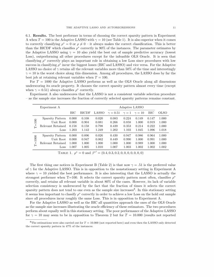
6.1. Results. The best performer in terms of choosing the correct sparsity pattern in ExperimentA when T = 100 is the Adaptive LASSO with γ = 10 (see Table 1). It is also superior when it comesto correctly classifying ρ∗ = 0 or ρ 6= 0 – it always makes the correct classification. This is betterthan the BICDF which classifies ρ∗ correctly in 90% of the instances. The parameter estimates bythe Adaptive LASSO using γ = 10 also yield the best out of sample predictive accuracy (lowestLoss), outperforming all other procedures except for the infeasible OLS Oracle. It is seen thatclassifying ρ∗ correctly plays an important role in obtaining a low Loss since procedures with lowsuccess in classifying ρ∗ incur the biggest losses (BIC and LASSO) and vice versa. For the AdaptiveLASSO no choice of γ retains all the relevant variables more than 50% of the time and interestinglyγ = 10 is the worst choice along this dimension. Among all procedures, the LASSO does by far thebest job at retaining relevant variables when T = 100.

For T = 1000 the Adaptive LASSO performs as well as the OLS Oracle along all dimensionsunderscoring its oracle property. It chooses the correct sparsity pattern almost every time (exceptwhen γ = 0.51) always classifies ρ∗ correctly.

Experiment A also underscores that the LASSO is not a consistent variable selection procedure– as the sample size increases the fraction of correctly selected sparsity patterns remains constant.

Experiment A Adaptive LASSO

BIC BICDF LASSO γ = 0.51 γ = 1 γ = 10 BIC OLSO

T=100 Sparsity Pattern 0.000 0.108 0.020 0.083 0.224 0.149 0.147 1.000

Unit Root 0.000 0.904 0.081 0.266 0.858 1.000 0.919 1.000Relevant Retained 0.158 0.158 0.798 0.439 0.353 0.214 0.222 1.000

Loss 1.203 1.142 1.249 1.202 1.103 1.045 1.096 1.018



Loss 1.007 1.005 1.010 1.007 1.003 1.002 1.002 1.002

Table 1. ρ∗ = 0 and β∗′ = (0.4, 0.3, 0.2, 0, 0, 0, 0, 0, 0, 0)

The first thing one notices in Experiment B (Table 2) is that now γ = .51 is the preferred valueof γ for the Adaptive LASSO. This is in opposition to the nonstationary setting in Experiment Awhere γ = 10 yielded the best performance. It is also interesting that the LASSO is actually thestrongest performer when T=100. It selects the correct sparsity pattern most often, classifies ρ∗

correctly, and retains all relevant variable in about 80% of the cases. However, its lack of variableselection consistency is underscored by the fact that the fraction of times it selects the correctsparsity pattern does not tend to one even as the sample size increases8. In this stationary settingit seems less important to classify ρ∗ correctly in order to achieve a low Loss on the hold out samplesince all procedures incur roughly the same Loss. This is in opposition to Experiment A.

For the Adaptive LASSO as well as the BIC all quantities approach the ones of the OLS Oracleas the sample size increases illustrating the oracle efficiency of these estimators. The two proceduresperform about equally well in this stationary setting. The poor performance of the Adaptive LASSOfor γ = 10 may seem to be in opposition to Theorem 2 but for T = 10.000 (results not reported

8The estimations were also carried out for T = 10.000 (not reported here) and even then the LASSO only detectedthe correct sparsity pattern in 47% of the instances.


here) the Adaptive LASSO detects the correct sparsity pattern in 92% of the instances even withthis value of γ.

Experiment B Adaptive LASSO




Loss 1.047 1.048 1.048 1.050 1.054 1.105 1.056 1.024



Loss 1.002 1.002 1.004 1.003 1.003 1.083 1.003 1.002

Table 2. ρ∗ = −0.05 and β∗′ = (0.4, 0.3, 0.2, 0, 0, 0, 0, 0, 0, 0)

As in Experiment A the data generating process possesses a unit root in Experiment C. Con-sidering the results for T=100 in Table 3 the findings from Experiment A are roughly confirmed.Choosing γ = 10 for the Adaptive LASSO seems to be a wise choice in the unit root setting evenwith gaps in the lag structure. The Adaptive LASSO always classifies ρ∗ correctly with this valueof γ and outperforms its closest competitor (the adaptive LASSO using BIC to choose γ by almost10%). By considering the Loss on the hold out sample it is also seen that a correct classification ofρ∗ results in a big gain in predictive power in the presence of a unit root confirming the finding inExperiment A.

As the sample size increases the the Adaptive LASSO and the BIC perform better while theperformance of the LASSO does not get better underscoring the oracle property of the first twoprocedures and the lack of the same for the LASSO. Note that the BICDF can not be expected toclassify ρ∗ correctly more often than in 95% of the cases in the presence of a unit root since testingis carried out at a 5% significance level. On the other hand, the correct classification probability ofthe Adaptive LASSO tends to one. Furthermore, the BIC is considerably slower to implement sincethe number of regressions to be run increases exponentially in the number of potential explanatoryvariables.

7. Conclusion

This paper has shown that the Adaptive LASSO can be tuned to perform consistent model se-lection in stationary and nonstationary autoregressions. The estimator of the parameters convergesat the oracle efficient rate, i.e. as fast as if an oracle had revealed the true model prior to estimationand only the relevant variables had bee included in a least squares estimation. This enables us touse the Adaptive LASSO to distinguish between stationary and nonstationary autoregressions.

However, the Adaptive LASSO has no power against alternatives in a shrinking neighborhoodaround 0 when tuned to perform consistent variable selection. This problem can be alleviated bytuning the Adaptive LASSO to perform conservative model selection. The price paid compared toconsistent model selection is that truly zero parameters are no longer set to zero with probabilitytending to one (but still with positive probability).


Experiment C Adaptive LASSO




Loss 1.242 1.158 1.298 1.233 1.133 1.083 1.132 1.033



Loss 1.008 1.006 1.012 1.010 1.005 1.003 1.003 1.003

Table 3. ρ∗ = 0 and β∗′ = (0.4, 0.3, 0.2, 0, 0, 0,−0.2, 0, 0, 0.2, 0, 0)

Monte Carlo experiments confirm that the Adaptive LASSO performs well compared to standardcompetitors. This is the case in particular for nonstationary data.

8. Appendix

Proof of Theorem 1. For the proof of this theorem we will need the following results which can befound in e.g. Hamilton (1994).

S−1T X ′TXTS

−1T →

(σ2

(1−∑pj=1 β

∗j )2

∫ 1

0W 2r dr 0

0 Σ

):= A,(5)

S−1T X ′T ε→

(σ2

(1−∑pj=1 βj)

∫ 1

0WrdWr

Z

):= B.(6)

We shall also make use of the fact that the least squares estimator, (ρI , β′I), of (ρ∗, β∗′) in (1)

satisfies that∥∥∥ST [(ρI , β′I)′ − (ρ∗, β∗′)′]∥∥∥

`2∈ Op(1)

First, let u = (u1, u′2)′ where u1 is a scalar and u2 a p × 1 vector. Set ρ = u1/T and βj =

β∗j + u2j/√T which implies that (2) as a function of u can be written as

ΨT (u) =

∥∥∥∥∥∆y − u1

Ty−1 −

p∑j=1

(β∗j +

u2j√T

)∆y−j

∥∥∥∥∥2

`2

+ λTwγ11

∣∣∣∣u1

T

∣∣∣∣+ λT

p∑j=1

wγ22j

∣∣∣∣β∗j +u2j√T

∣∣∣∣ .Let u = (u1, u

′2)′ = arg min ΨT (u) and notice that u1 = T ρ and u2j =

√T (βj−β∗j ) for j = 1, ..., p.

Define


VT (u) = ΨT (u)−ΨT (0)

= u′S−1T X ′TXTS

−1T u− 2u′S−1

T X ′T ε+ λTwγ11

∣∣∣∣u1

T

∣∣∣∣+ λT

p∑j=1

wγ22j

(∣∣∣∣β∗j +u2j√T

∣∣∣∣−∣∣∣β∗j ∣∣∣).

Consider the first two terms in the above display. It follows from (5) and (6) that

u′S−1T X ′TXTS

−1T u− 2u′S−1

T X ′T ε→u′Au− 2u′B.(7)

Furthermore,

λTwγ11

∣∣∣∣u1

T

∣∣∣∣ = λT1

|ρI |γ1

∣∣∣∣u1

T

∣∣∣∣ = |u1|λT

T 1−γ11

|T ρI |γ1→

{∞ in probability if u1 6= 0

0 in probability if u1 = 0(8)

since T ρI is tight. Also, if β∗j 6= 0

λTwγ22j

(∣∣∣∣β∗j +u2j√T

∣∣∣∣−∣∣∣β∗j ∣∣∣)

= λT

∣∣∣∣ 1

βI,j

∣∣∣∣γ2 u2j√T

(∣∣∣∣β∗j +u2j√T

∣∣∣∣−∣∣∣β∗j ∣∣∣)/( u2j√

T

)=

λTT 1/2

∣∣∣∣ 1

βI,j

∣∣∣∣γ2 u2j

(∣∣∣∣β∗j +u2j√T

∣∣∣∣−∣∣∣β∗j ∣∣∣)/( u2j√

T

)→ 0 in probability(9)

since (i): λT /T1/2 → 0, (ii):

∣∣1/βI,j∣∣γ2 → ∣∣1/β∗j ∣∣γ2 <∞ in probability and

(iii): u2j

(∣∣∣β∗j +u2j√T

∣∣∣−∣∣∣β∗j ∣∣∣) /( u2j√T

)→ u2jsign(β∗j ).

Finally, if β∗j = 0,

λTwγ22j

(∣∣∣∣β∗j +u2j√T

∣∣∣∣−∣∣∣β∗j ∣∣∣)

=λTT 1/2

∣∣∣∣ 1

βI,j

∣∣∣∣γ2∣∣u2j

∣∣ =λT

T 1/2−γ2/2

∣∣∣∣∣ 1√T βI,j

∣∣∣∣∣γ2∣∣u2j

∣∣→

{∞ in probability if u2j 6= 0

0 in probability if u2j = 0(10)

since (i): λTT 1/2−γ2/2 →∞ and (ii):

√T βI,j is tight.

Putting together (7)-(10) one concludes:

VT (u)→Ψ(u) =

{u′Au− 2u′B if u1 = 0 and u2j = 0 for all j ∈ Ac

∞ if u1 6= 0 or u2j 6= 0 for some j ∈ Ac

Since VT (u) is convex and Ψ(u) has a unique minimum it follows from Knight (1999) thatarg minVT (u)→ arg min Ψ(u). Hence,


u1→δ0(11)

u2Ac→δ|Ac|

0(12)

u2A→N(0, σ2[ΣA]−1)(13)

where δ0 is the Dirac measure at 0 and |Ac| is the cardinality of Ac (hence, δ|Ac|0 is the |Ac|-

dimensional Dirac measure at 0). Notice that (11) and (12) imply that u1 → 0 in probability andu2Ac → 0 in probability. An equivalent formulation of (11)-(13) is

T ρ→δ0(14)√T (βAc − β∗Ac)→δ

|Ac|0(15)

√T (βA − β∗A)→N(0, σ2[ΣA]−1)(16)

(14)-(16) yield the consistency part of the theorem at the rate of T for ρ and√T for β. Notice

that this also implies that no βj , j ∈ A will be set equal to 0 since for all j ∈ A, βj converges inprobability to β∗j 6= 0. (16) also yields the oracle efficient asymptotic distribution, i.e. part (3) of

the theorem. It remains to show part (2) of the theorem; P (ρT = 0) → 1 and P (βT,Ac = 0) → 1.Both proofs are by contradiction.

First, assume ρ 6= 0. Then the first order conditions for a minimum read:

2y′−1

(∆y −XT (ρ, β′)′

)+ λTw

γ11 sign(ρ) = 0

which is equivalent to

2y′−1

(∆y −XT (ρ, β′)′

)T

+λTw

γ11 sign(ρ)

T= 0

Consider first the second term:∣∣∣∣∣λTwγ11 sign(ρ)

T

∣∣∣∣∣ =λT

T 1−γ11

|T ρI |γ1→∞ in probability

since T ρI is tight. For the first term one has:

2y′−1

(∆y −XT (ρ, β′)′

)T

=2y′−1

(ε−XTS

−1T ST [ρ, β′ − β∗′]′

)T

=2y′−1ε

T−

2y′−1XTS−1T ST [ρ, β′ − β∗′]′

T

By (6),y′−1ε

T →σ2

1−∑pj=1 β

∗j

∫ 1

0WrdWr. Furthermore,

y′−1XTS−1T

T →((

σ1−

∑pj=1 β

∗j

)2 ∫ 1

0W 2r dr, 0, ..., 0

)by (5). Hence,

y′−1ε

T andy′−1XTS

−1T

T are tight. We also know that ST [ρT , β′T −β∗

′]′ converges weakly

by (14)-(16) which implies it is tight as well. Taken together,2y′−1(∆y−XT (ρT ,β

′T )′)

T is tight and so


P (ρT 6= 0) ≤ P

(2y′−1

(∆y −XT (ρT , β

′T )′)

T+λTw

γ11 sign(ρT )

T= 0

)→ 0

Next, assume βj 6= 0 for j ∈ Ac. From the first order conditions

∆y′−j(∆y −XT (ρ, β′)′) + λTwγ22j sign(βj) = 0

or equivalently,

2∆y′−j

(∆y −XT (ρ, β′)′

)T 1/2

+λTw

γ22j sign(βj)

T 1/2= 0

First, consider the second term

∣∣∣∣∣∣λTwγ22j sign(βj)

T 1/2

∣∣∣∣∣∣ =λTw

γ22j

T 1/2=

λT

T 1/2−γ2/2 |T 1/2βI,j |γ2 →∞

since√T βI,j is tight. Regarding the first term,

2∆y′−j

(∆y −XT (ρ, β′)′

)T 1/2

=2∆y′−j

(ε−XTS

−1T ST [ρT , β

′ − β∗′]′)

T 1/2

=2∆y′−jε

T 1/2−

2∆y′−jXTS−1T ST [ρ, β′ − β∗′]′

T 1/2

By (6)∆y′−jε

T 1/2 →N(0, σ2Σj) where in accordance with previous notation Σj is the jth diagonal

element of Σ.∆y′−jXTS

−1T

T 1/2 →(0,Σ(j,1), ...,Σ(j,p)) by (5). Hence,∆y′−jε

T 1/2 and∆y′−jXTS

−1T

T 1/2 are tight.

The same is the case for ST [ρ, β′ − β∗′] since it converges weakly by (14)-(16). Taken together,2∆y′−j(∆y−XT (ρ,β′)′)

T 1/2 is tight and so

P (βj 6= 0) ≤ P

(2∆y′−j

(∆y −XT (ρ, β′)′

)T 1/2

+λTw

γ22j sign(ρT )

T 1/2= 0

)→ 0

�

Proof of Theorem 2. The proof runs along the same lines as the proof of Theorem 1. For the proofwe will need (17) and (18) below which can be found in e.g. Hamilton (1994), Chapter 8. Noticethat by definition of xt = (yt−1, z

′t)′ the lower right hand (p× p) block of Q is Σ.

We shall make use of the following limit results:


1

TX ′TXT

p→ Q(17)

1√TX ′T ε→Np+1(0, σ2Q) := B(18)

where the definition of B means that B is a random vector distributed as Np+1(0, σ2Q) We shall

also make use of the fact that the least squares estimator is√T consistent under stationarity, i.e.∥∥∥√T [(ρI , β′I)′ − (ρ∗, β∗′)′]∥∥∥

`2∈ Op(1)

First, let u = (u1, u′2)′ where u1 is a scalar and u2 a p × 1 vector. Set ρ = ρ∗ + u1/

√T and

βj = β∗j + u2j/√T and

ΨT (u) =

∥∥∥∥∥∆y −(ρ∗ +

u1√T

)y−1 −

p∑j=1

(β∗j +

u2j√T

)∆y−j

∥∥∥∥∥2

`2

+ λTwγ11

∣∣∣∣ρ∗ +u1√T

∣∣∣∣+ λT

p∑j=1

wγ22j

∣∣∣∣β∗j +u2j√T

∣∣∣∣Let u = (u1, u

′2)′ = arg min ΨT (u) and notice that u1 =

√T (ρ− ρ∗) and u2j =

√T (βj − β∗j ) for

j = 1, ..., p. Define

VT (u) = ΨT (u)−ΨT (0)

=1

Tu′X ′TXTu− 2

1√Tu′X ′T ε+ λTw

γ11

(∣∣∣∣ρ∗ +u1√T

∣∣∣∣−|ρ∗|)

+ λT

p∑j=1

wγ22j

(∣∣∣∣β∗j +u2j√T

∣∣∣∣−∣∣∣β∗j ∣∣∣)

Consider the first two terms in the above display. It follows from (17) and (18) that

1

Tu′X ′TXTu− 2

1√Tu′X ′T ε→u′Qu− 2u′B(19)

Furthermore, since ρ∗ 6= 0

λTwγ11

(∣∣∣∣ρ∗ +u1√T

∣∣∣∣−|ρ∗|)

= λT

∣∣∣∣ 1

ρI

∣∣∣∣γ1 u1√T

(∣∣∣∣ρ∗ +u1√T

∣∣∣∣−|ρ∗|)/( u1√

T

)=

λTT 1/2

∣∣∣∣ 1

ρI

∣∣∣∣γ1 u1

(∣∣∣∣ρ∗ +u1√T

∣∣∣∣−|ρ∗|)/( u1√

T


since (i): λT /T1/2 → 0, (ii):

∣∣1/ρI ∣∣γ1 → ∣∣1/ρ∗∣∣γ1 <∞ in probability and

(iii): u1

(∣∣∣ρ∗ + u1√T

∣∣∣−|ρ∗|) /( u1√T

)→ u1sign(ρ∗).


Similarly, if β∗j 6= 0

λTwγ22j

(∣∣∣∣β∗j +u2j√T

∣∣∣∣−∣∣∣β∗j ∣∣∣)

= λT

∣∣∣∣ 1

βI,j

∣∣∣∣γ2 u2j√T

(∣∣∣∣β∗j +u2j√T

∣∣∣∣−∣∣∣β∗j ∣∣∣)/( u2j√

T

)=

λTT 1/2

∣∣∣∣ 1

βI,j

∣∣∣∣γ2 u2j

(∣∣∣∣β∗j +u2j√T

∣∣∣∣−∣∣∣β∗j ∣∣∣)/( u2j√

T


since (i): λT /T1/2 → 0, (ii):

∣∣1/βI,j∣∣γ2 → ∣∣1/β∗j ∣∣γ2 <∞ in probability and

(iii): u2j

(∣∣∣β∗j +u2j√T

∣∣∣−∣∣∣β∗j ∣∣∣) /( u2j√T



λTwγ22j

(∣∣∣∣β∗j +u2j√T

∣∣∣∣−∣∣∣β∗j ∣∣∣)

=λTT 1/2

∣∣∣∣ 1

βI,j

∣∣∣∣γ2∣∣u2j

∣∣ =λT

T 1/2−γ2/2

∣∣∣∣∣ 1√T βI,j

∣∣∣∣∣γ2∣∣u2j

∣∣→

{∞ in probability if u2j 6= 0

0 in probability if u2j = 0(22)

since (i): λTT 1/2−γ2/2 →∞ and (ii)

√T βI,j is tight.

Putting (19)-(22) together one concludes:

VT (u)→Ψ(u) =

{u′Qu− 2u′B if u2j = 0 for all j ∈ Ac

∞ if u2j 6= 0 for some j ∈ Ac

Since VT (u) is convex and Ψ(u) has a unique minimum it follows from Knight (1999) that

arg min VT (u)→ arg min Ψ(u). Hence,

(u1, u′2A)′→N

(0, σ2[Q(1,A+1)]

−1)

(23)

u2Ac→δ|Ac|

0(24)

where δ0 is the Dirac measure at 0 and |Ac| is the cardinality of Ac (hence, δ|Ac|0 is the |Ac|-

dimensional Dirac measure at 0). Notice that (24) implies that u2Ac → 0 in probability. Anequivalent formulation of (23) and (24) is( √

T (ρ− ρ∗)√T (βA − β∗A)

)→N

(0, σ2[Q(1,A+1)]

−1)

(25)

√T (βAc − β∗Ac)→δ

|Ac|0(26)

(25) and (26) establish the consistency part of the theorem at the oracle rate of√T . Note

that this also implies that for no j ∈ A will βj be set equal to 0 since for each j ∈ A, βjconverges in probability to β∗j 6= 0. The same is true for ρ. (25) also yields the oracle efficientasymptotic distribution, i.e. part (3) of the theorem. It remains to show part (2) of the theorem;

P (βAc = 0)→ 1. The proof is by contradiction.


Assume βj 6= 0 for j ∈ Ac. From the first order conditions

2∆y′−j(∆y −XT (ρ, β′)′) + λTwγ22j sign(βj) = 0

or equivalently,

2∆y′−j

(∆y −XT (ρ, β′)′

)T 1/2

+λTw

γ22j sign(βj)

T 1/2= 0

First, consider the second term

∣∣∣∣∣∣λTwγ22j sign(βj)

T 1/2

∣∣∣∣∣∣ =λTw

γ22j

T 1/2=

λT

T 1/2−γ2/2 |T 1/2βI,j |γ2 →∞

since√T βI,j is tight. Regarding the first term,

2∆y′−j

(∆y −XT (ρ, β′)′

)T 1/2

=2∆y′−j

(ε−XT [ρ− ρ∗, β′ − β∗′]′

)T 1/2

=2∆y′−jε

T 1/2−

2∆y′−jXT

√T [ρ− ρ∗, β′ − β∗′]′

T

By (18),∆y′−jε

T 1/2 →N(0, σ2Q(j+1)) where in accordance with previous notation Q(j+1) is the (j +

1)th diagonal element of Q.∆y′−jXT

T

p→ (Q(j+1,1), ..., Q(j+1,p+1)) by (17). Hence,∆y′−jε

T 1/2 and∆y′−jXT

T

are tight. The same is the case for√T [ρ−ρ∗, β′−β∗′] since it converges weakly by (25)-(26). Hence,

P (βj 6= 0) ≤ P

(2∆y′−j

(∆y −XT (ρT , β

′T )′)

T 1/2+λTw

γ22j sign(ρT )

T 1/2= 0

)→ 0

�

Before proving Theorem 3 we prove the following lemma. Let (x)+ = max(x, 0).

Lemma 1. Let g : R→ R be given by g(u) = u2 − 2au+ 2λ|u| , λ ≥ 0, a 6= 0. Then arg min g = 0if and only if λ ≥|a|. More precisely, arg min g = sign(a)

(|a| − λ

)+

.

Proof. Assume a > 0. Since g′(u) = 2u − 2a + 2λsign(u) is strictly negative for u < 0 arg min g ∈[0,∞). u > 0 is a local minimum (and hence a global minimum since g is strictly convex) if and onlyif it is a stationary point, i.e. g′(u) = 2u−2a+2λ = 0 which is equivalent to 0 < u = a−λ = |a|−λ.This contradicts λ ≥ |a| and so arg min g = 0 when λ ≥ |a|. In total, the above shows thatarg min g = (a− λ)+ = sign(a)

(|a| − λ

)+

for a > 0. Similar arguments establish the result fora < 0.

�


Proof of Theorem 3. ρ minimizes

L(ρ) =

T∑t=1

(∆yt − ρyt−1)2 + 2λT|ρ|∣∣ρI ∣∣ =

T∑t=1

∆y2t + ρ2

T∑t=1

y2t−1 − 2ρ

T∑t=1

∆ytyt−1 + 2λT|ρ|∣∣ρI ∣∣

which is equvalent to minimizing

ρ2 − 2ρ

∑Tt=1 ∆ytyt−1∑Tt=1 y

2t−1

+ 2λT|ρ|∣∣ρI ∣∣∑Tt=1 y

2t−1

= ρ2 − 2ρρI + 2λT|ρ|∣∣ρI ∣∣∑Tt=1 y

2t−1

It follows from Lemma 1 that ρ = 0 if and only if

∣∣ρI ∣∣ ≤ λT

|ρI |∑Tt=1 y

2t−1

⇔ ρI2T∑t=1

y2t−1 ≤ λT

Hence, recalling that ρI =∑Tt=1 ∆ytyt−1/

∑Tt=1 y

2t−1 (the least squares estimator)

P (ρ = 0) = P

(ρ2I

T∑t=1

y2t−1 ≤ λT

)= P

([∑Tt=1 ∆ytyt−1∑Tt=1 y

2t−1

]2 T∑t=1

y2t−1 ≤ λT

)

= P

([ρ∗ +

∑Tt=1 yt−1εt∑Tt=1 y

2t−1

]2 T∑t=1

y2t−1 ≤ λT

)

= P

(ρ∗2 +

[∑Tt=1 yt−1εt∑Tt=1 y

2t−1

]2

+ 2ρ∗∑Tt=1 yt−1εt∑Tt=1 y

2t−1

T∑t=1

y2t−1 ≤ λT

)�

Proof of Theorem 4. From Phillips (1987a) one has

( 1

T

T∑t=1

yt−1εt,1

T 2

T∑t=1

y2t−1

)→(σ2

∫ 1

0

WsdWs, σ2

∫ 1

0

W 2s ds

)(27)

Using Theorem 3 with ρ∗ = 0 yields

P (ρ = 0) = P

([1T

∑Tt=1 yt−1εt

1T 2

∑Tt=1 y

2t−1

]21

T 2

T∑t=1

y2t−1 ≤ λT

)From (27) and the continuous mapping theorem it follows that

GT :=

[1T

∑Tt=1 yt−1εt

1T 2

∑Tt=1 y

2t−1

]21

T 2

T∑t=1

y2t−1→

∫ 1

0WsdWs∫ 1

0W 2s ds

2

σ2

∫ 1

0

W 2s ds := G(28)

where the last definition means thatG is a random variable distributed as

[ ∫ 10WsdWs∫ 1

0W 2s ds

]2

σ2∫ 1

0W 2s ds.


Case 1: λT → 0. Since the right hand side in (28) is absolutely continuous with respect to theLebesgue measure it has no mass points and so

P (ρ = 0) = P(GT ≤ λT

)= FGT (λT )→ FG(0) = 0

if λT → 0.Case 2:λT → λ ∈ (0,∞). By the same reasoning as in case 1 it follows that

P (ρ = 0) = P(GT ≤ λT

)= FGT (λT )→ FG(λ) = p ∈ (0, 1)

since G is supported on all of R+.Case 3: λT →∞. Since GT converges weakly it is tight and the result follows. �

Proof of Theorem 5. By standard results (see e.g. Hamilton (1994))

1

T 1/2

T∑t=1

yt−1εt→N(0, σ2E[y2t−1])

1

T

T∑t=1

y2t−1

p→ E(y2t−1)

Using Theorem 3 with ρ∗ ∈ (−2, 0) yields

P (ρ = 0) = P

Tρ∗2 +

1T 1/2

∑Tt=1 yt−1εt

1T

∑Tt=1 y

2t−1

2

+ 2T 1/2ρ1

T 1/2

∑Tt=1 yt−1εt

1T

∑Tt=1 y

2t−1

1

T

T∑t=1

y2t−1 ≤ λT

= P

ρ∗2 +

1

T

1T 1/2

∑Tt=1 yt−1εt

1T

∑Tt=1 y

2t−1

2

+ 21

T 1/2ρ

1T 1/2

∑Tt=1 yt−1εt

1T

∑Tt=1 y

2t−1

1

T

T∑t=1

y2t−1 ≤

λTT

Since

1

T1/2

∑Tt=1 yt−1εt

1T

∑Tt=1 y

2t−1

is tight it follows that

1

T

1T 1/2

∑Tt=1 yt−1εt

1T

∑Tt=1 y

2t−1

2

+ 21

T 1/2ρ

1T 1/2

∑Tt=1 yt−1εt

1T

∑Tt=1 y

2t−1

p→ 0

which implies that

HT :=

ρ∗2 +1

T

1T 1/2

∑Tt=1 yt−1εt

1T

∑Tt=1 y

2t−1

2

+ 21

T 1/2ρ

1T 1/2

∑Tt=1 yt−1εt

1T

∑Tt=1 y

2t−1

1

T

T∑t=1

y2t−1

p→ ρ∗2E(y2t−1) := L

Case 1: λT /T → 0. Since HT converges in probability to L it follows that

P (ρ = 0) = P (HT ≤ λT /T ) ≤ P (HT ≤ L− L/2)→ 0


where the estimate holds for T sufficiently large since λT /T → 0.Case 2: λT /T → λ ∈ (0,∞).

P (ρ = 0) = P(HT ≤ λT

){≤ P (HT ≤ λ+ (L− λ)/2) ≤ P (HT ≤ L− (L− λ)/4)→ 0, λ < L

≥ P (HT ≤ λ− (λ− L)/2) ≥ P (HT ≤ L+ (λ− L)/4)→ 1, λ > L

where the first estimate in each of the cases holds from a certain step and onwards.Case 3: λT /T →∞. Since HT converges in probability it is tight and the result follows.

�

Proof of Theorem 6. By Phillips (1987b)

(1

T

T∑t=1

yt−1εt,1

T 2

T∑t=1

y2t−1

)→(σ2

∫ 1

0

Jc(r)dW (r), σ2

∫ 1

0

J2c (r)dr

)(29)

where Jc is the Ornstein-Uhlenbeck process with parameter c. Notice how the only difference to(27) is that the integrand process now is Jc(r) instead of W (r). For c = 0 they are identical as theOrnstein-Uhlenbeck process collapses to the Wiener process.

From Theorem 3 with ρ∗ = c/T it follows

P (ρ = 0) = P

((c/T )2 +

[∑Tt=1 yt−1εt∑Tt=1 y

2t−1

]2

+ 2c/T

∑Tt=1 yt−1εt∑Tt=1 y

2t−1

T∑t=1

y2t−1 ≤ λT

)

= P

(c2 +

[1T

∑Tt=1 yt−1εt

1T 2

∑Tt=1 y

2t−1

]2

+ 2c1T

∑Tt=1 yt−1εt

1T 2

∑Tt=1 y

2t−1

1

T 2

T∑t=1

y2t−1 ≤ λT

)By the continuous mapping theorem

KT :=

c2 +

[1T

∑Tt=1 yt−1εt

1T 2

∑Tt=1 y

2t−1

]2

+ 2c1T

∑Tt=1 yt−1εt

1T 2

∑Tt=1 y

2t−1

1

T 2

T∑t=1

y2t−1

→

c2 +

∫ 1

0Jc(r)dW (r)∫ 1

0J2c (r)dr

2

+ 2c

∫ 1

0Jc(r)dW (r)∫ 1

0J2c (r)dr

σ2

∫ 1

0

J2c (r)dr := K

where the last definition means that K is a random variable distributed as the weak limit of KT .Case 1: λT → 0. Since K is absolutely continuous with respect to the Lebesgue measure it has

no mass points and so

P (ρ = 0) = P (KT ≤ λT ) = FKT (λT )→ FK(0) = 0

Case 2: λT → λ ∈ (0,∞). By the same reasoning as in Case 1 it follows that

P (ρ = 0) = P (KT ≤ λT ) = FKT (λT )→ FK(λ) ∈ (0, 1)

since K is supported on all of R+.Case 3: λT →∞. Since KT converges weakly it is tight and the result follows.

�


Proof of Theorem 7. The setting is the same as in the proof of Theorem 1. Follow the proof of thattheorem, with identical notation, until (7) with γ1 = γ2 = 1. Next, notice that

λTw1

∣∣∣∣u1

T

∣∣∣∣ = λT1

|ρI |

∣∣∣∣u1

T

∣∣∣∣ = |u1|λT1

|T ρI |→λ |u1||C1|

(30)

by (5) and (6) since C1 has no mass at 0.Furthermore, if β∗j 6= 0

λTw2j

(∣∣∣∣β∗j +u2j√T

∣∣∣∣−∣∣∣β∗j ∣∣∣)

= λT

∣∣∣∣ 1

βI,j

∣∣∣∣ u2j√T

(∣∣∣∣β∗j +u2j√T

∣∣∣∣−∣∣∣β∗j ∣∣∣)/( u2j√

T

)=

λTT 1/2

∣∣∣∣ 1

βI,j

∣∣∣∣u2j

(∣∣∣∣β∗j +u2j√T

∣∣∣∣−∣∣∣β∗j ∣∣∣)/( u2j√

T


since (i): λT /T1/2 → 0, (ii):

∣∣1/βI,j∣∣→ ∣∣1/β∗j ∣∣ <∞ in probability and (iii):

u2j

(∣∣∣β∗j +u2j√T

∣∣∣−∣∣∣β∗j ∣∣∣) /( u2j√T



λTw2j

(∣∣∣∣β∗j +u2j√T

∣∣∣∣−∣∣∣β∗j ∣∣∣)

=λTT 1/2

∣∣∣∣ 1

βI,j

∣∣∣∣∣∣u2j

∣∣ = λT

∣∣∣∣∣ 1√T βI,j

∣∣∣∣∣∣∣u2j

∣∣ →λ |u2j ||C2j |

(32)

by (5) and (6) since (i): λT → λ and (ii): C2j is 0 with probability 0 such that x 7→∣∣1/x∣∣ is

continuous almost everywhere with respect to the limiting measure.Putting together (7) and(30)-(32) one concludes

VT (u)→u′Au− 2u′B + λ|u1||C1|

+ λ

p∑j=1

|u2j ||C2j |

1{β∗j=0

} := Ψ(u)

Hence, since VT (u) is convex and Ψ(u) has a unique minimum it follows from Knight (1999) thatarg minVT (u)→ arg min Ψ(u)

�

Proof of Theorem 8. The setting is the same as in the proof of Theorem 2. Follow the proof of thattheorem, with identical notation, until (21) with γ1 = γ2 = 1. For the case of β∗j = 0 one has

λTw2j

(∣∣∣∣β∗j +u2j√T

∣∣∣∣−∣∣∣β∗j ∣∣∣)

=λTT 1/2

∣∣∣∣ 1

βI,j

∣∣∣∣∣∣u2j

∣∣ = λT

∣∣∣∣∣ 1√T βI,j

∣∣∣∣∣∣∣u2j

∣∣ →λ |u2j ||C2j |

(33)

by (17) and (18) since (i): λT → λ, (ii): C2j is 0 with probability 0 such that x 7→∣∣1/x∣∣ is

continuous almost everywhere with respect to the limiting measure.Putting together (19)-(21) and (33) one concludes

VT (u)→u′Qu− 2u′B + λ

p∑j=1

|u2j ||C2j |

1{β∗j=0

} := Ψ(u)


Hence, since VT (u) is convex and Ψ(u) has a unique minimum it follows from Knight (1999) that

arg min VT (u)→ arg min Ψ(u)�

References

Buhlmann, P. and S. Van De Geer (2011). Statistics for High-Dimensional Data: Methods, Theoryand Applications. Springer-Verlag, New York.

Candes, E. and T. Tao (2007). The dantzig selector: Statistical estimation when p is much largerthan n. The Annals of Statistics 35, 2313–2351.

Efron, B., T. Hastie, I. Johnstone, and R. Tibshirani (2004). Least angle regression. The Annalsof statistics 32, 407–499.

Fan, J. and R. Li (2001). Variable selection via nonconcave penalized likelihood and its oracleproperties. Journal of the American Statistical Association 96, 1348–1360.

Fan, J. and J. Lv (2008). Sure independence screening for ultrahigh dimensional feature space.Journal of the Royal Statistical Society: Series B (Statistical Methodology) 70, 849–911.

Hamilton, J. D. (1994). Time Series Analysis. Cambridge University Press, Cambridge.Huang, J., J. L. Horowitz, and S. Ma (2008). Asymptotic properties of bridge estimators in sparse

high-dimensional regression models. The Annals of Statistics 36, 587–613.Knight, K. (1999). Epi-convergence in distribution and stochastic equi-semicontinuity. Unpublished

manuscript .Knight, K. and W. Fu (2000). Asymptotics for lasso-type estimators. Annals of Statistics, 1356–

1378.Knight, K. and W. Fu (2011). An alternative to unit root tests: Bridge estimators differentiate

between nonstationary versus stationary models and select optimal lag. Working paper .Kock, A. B. (2012). Oracle efficient variable selection in random and fixed effects panel data models.

Econometric Theory (forthcoming).Leeb, H. and B. Potscher (2008). Sparse estimators and the oracle property, or the return of hodges’

estimator. Journal of Econometrics 142, 201–211.Leeb, H. and B. M. Potscher (2005). Model selection and inference: Facts and fiction. Econometric

Theory 21, 21–59.Lehmann, E. L. and G. Casella (1998). Theory of point estimation, Volume 31. Springer Verlag.Meinshausen, N. and P. Buhlmann (2006). High-dimensional graphs and variable selection with the

lasso. The Annals of Statistics 34, 1436–1462.Ng, S. and P. Perron (2001). Lag length selection and the construction of unit root tests with good

size and power. Econometrica 69, 1519–1554.Phillips, P. C. B. (1987a). Time series regression with a unit root. Econometrica, 277–301.Phillips, P. C. B. (1987b). Towards a unified asymptotic theory for autoregression. Biometrika 74,

535–547.Potscher, B. and H. Leeb (2009). On the distribution of penalized maximum likelihood estimators:

The lasso, scad, and thresholding. Journal of Multivariate Analysis 100, 2065–2082.Tibshirani, R. (1996). Regression shrinkage and selection via the lasso. Journal of the Royal

Statistical Society. Series B (Methodological), 267–288.Wang, H., G. Li, and C. L. Tsai (2007). Regression coefficient and autoregressive order shrink-

age and selection via the lasso. Journal of the Royal Statistical Society: Series B (StatisticalMethodology) 69, 63–78.


Zhao, P. and B. Yu (2006). On model selection consistency of lasso. The Journal of MachineLearning Research 7, 2541–2563.

Zou, H. (2006). The adaptive lasso and its oracle properties. Journal of the American StatisticalAssociation 101, 1418–1429.

Research Papers

2012

2011-43: Peter Christoffersen, Ruslan Goyenko, Kris Jacobs, Mehdi Karoui: Illiquidity Premia in the Equity Options Market

2011-44: Diego Amaya, Peter Christoffersen, Kris Jacobs and Aurelio Vasquez: Do Realized Skewness and Kurtosis Predict the Cross-Section of Equity Returns?

2011-45: Peter Christoffersen and Hugues Langlois: The Joint Dynamics of Equity Market Factors

2011-46: Peter Christoffersen, Kris Jacobs and Bo Young Chang: Forecasting with Option Implied Information

2011-47: Kim Christensen and Mark Podolskij: Asymptotic theory of range-based multipower variation

2011-48: Christian M. Dahl, Daniel le Maire and Jakob R. Munch: Wage Dispersion and Decentralization of Wage Bargaining

2011-49: Torben G. Andersen, Oleg Bondarenko and Maria T. Gonzalez-Perez: Coherent Model-Free Implied Volatility: A Corridor Fix for High-Frequency VIX

2011-50: Torben G. Andersen and Oleg Bondarenko: VPIN and the Flash Crash

2011-51: Tim Bollerslev, Daniela Osterrieder, Natalia Sizova and George Tauchen: Risk and Return: Long-Run Relationships, Fractional Cointegration, and Return Predictability

2011-52: Lars Stentoft: What we can learn from pricing 139,879 Individual Stock Options

2011-53: Kim Christensen, Mark Podolskij and Mathias Vetter: On covariation estimation for multivariate continuous Itô semimartingales with noise in non-synchronous observation schemes

2012-01: Matei Demetrescu and Robinson Kruse: The Power of Unit Root Tests Against Nonlinear Local Alternatives

2012-02: Matias D. Cattaneo, Michael Jansson and Whitney K. Newey: Alternative Asymptotics and the Partially Linear Model with Many Regressors

2012-03: Matt P. Dziubinski: Conditionally-Uniform Feasible Grid Search Algorithm

2012-04: Jeroen V.K. Rombouts, Lars Stentoft and Francesco Violante: The Value of Multivariate Model Sophistication: An Application to pricing Dow Jones Industrial Average options

2012-05: Anders Bredahl Kock: On the Oracle Property of the Adaptive LASSO in Stationary and Nonstationary Autoregressions

On the Oracle Property of the Adaptive LASSO in...

Documents

Transcript of On the Oracle Property of the Adaptive LASSO in...