NBER WORKING PAPER SERIES

ON THE OPTIMAL PROVISION OF SOCIAL INSURANCE:PROGRESSIVE TAXATION VERSUS EDUCATION SUBSIDIES IN GENERAL EQUILIBRIUM

Dirk KruegerAlexander Ludwig

Working Paper 21538http://www.nber.org/papers/w21538

NATIONAL BUREAU OF ECONOMIC RESEARCH1050 Massachusetts Avenue

Cambridge, MA 02138September 2015

We thank Felicia Ionescu, Costas Meghir, Dominik Sachs and Gianluca Violante for helpful discussionsand seminar participants at various institutions and conferences for many useful comments. Kruegergratefully acknowledges financial support from the NSF under grant SES-0820494. Ludwig gratefullyacknowledges financial support by the Research Center SAFE, funded by the State of Hessen initiativefor research LOEWE. The views expressed herein are those of the authors and do not necessarily reflectthe views of the National Bureau of Economic Research.

NBER working papers are circulated for discussion and comment purposes. They have not been peer-reviewed or been subject to the review by the NBER Board of Directors that accompanies officialNBER publications.

© 2015 by Dirk Krueger and Alexander Ludwig. All rights reserved. Short sections of text, not toexceed two paragraphs, may be quoted without explicit permission provided that full credit, including© notice, is given to the source.

On the Optimal Provision of Social Insurance: Progressive Taxation versus Education Subsidiesin General EquilibriumDirk Krueger and Alexander LudwigNBER Working Paper No. 21538September 2015JEL No. E62,H21,H24

ABSTRACT

In this paper we compute the optimal tax and education policy transition in an economy where progressivetaxes provide social insurance against idiosyncratic wage risk, but distort the education decision ofhouseholds. Optimally chosen tertiary education subsidies mitigate these distortions. We highlightthe quantitative importance of general equilibrium feedback effects from policies to relative wagesof skilled and unskilled workers: subsidizing higher education increases the share of workers witha college degree thereby reducing the college wage premium which has important redistributive benefits.We also argue that a full characterization of the transition path is crucial for policy evaluation. Wefind that optimal education policies are always characterized by generous tuition subsidies, but theoptimal degree of income tax progressivity depends crucially on whether transitional costs of policiesare explicitly taken into account and how strongly the college premium responds to policy changesin general equilibrium.

Dirk KruegerEconomics DepartmentUniversity of Pennsylvania160 McNeil Building3718 Locust WalkPhiladelphia, PA 19104and NBERdkrueger@econ.upenn.edu

Alexander LudwigGoethe University FrankfurtHouse of FinanceTheodor-W.-Adorno-Platz 3D-60629 Frankfurt am MainLudwig@safe.uni-frankfurt.de

1 Introduction

In the presence of uninsurable idiosyncratic earnings risk, progressive taxation pro-

vides valuable social insurance among ex ante identical households. In addition it

might enhance equity among ex ante heterogeneous households, which is beneficial

if the social welfare function used to aggregate lifetime utilities values such equity.

However, if high-earnings households face higher average tax rates than low-earnings

households, this might discourage the incentives of these households to become earnings-

rich through making conscious human capital accumulation decisions. The resulting

skill distribution in the economy worsens, and aggregate economic activity might be

depressed through this channel, which compounds the potentially adverse impact of

progressive taxes on production through the classic labor supply channel.

In this paper we compute the optimal tax and education policy transition, within a

simple parametric class, in an economy where progressive taxes provide social insur-

ance against idiosyncratic wage risk, but distort the education decision of households.

Optimally chosen tertiary education subsidies mitigate these distortions, making both

policies potentially complementary. We model two different channels through which

academic talent is transmitted across generations (persistence of innate ability vs. the

impact of parental education) and permit different forms of labor to be imperfect sub-

stitutes, thereby generating general equilibrium feedback effects from policies to rela-

tive wages of skilled and unskilled workers.

We show that subsidizing higher education has important redistributive benefits, by

shrinking the college wage premium in general equilibrium. This Stiglitz (1982) ef-

fect of fiscal policy on relative factor prices may make progressive taxes and education

subsidies potential policy substitutes for providing social insurance.1 We also argue that

a full characterization of the transition path is crucial for policy evaluation. In our

quantitative analysis we find that optimal education policies are always characterized

by generous tuition subsidies. The optimal degree of income tax progressivity how-

ever crucially depends on whether transitional costs of policies are explicitly taken

into account and how strongly the college wage premium responds to policy changes

in general equilibrium.

Our benchmark economy models skilled and unskilled labor as imperfect substitutes

in the production of final output, following the empirical literature since Katz and

Murphy (1992) or Borjas (2003), with a substitution elasticity of 1.4. When maximizing

utilitarian social welfare valuing transitional generations in this economy, we docu-

ment in section 6.2.1 that the optimal policy is characterized by a massive education

1 Heathcote, Storesletten and Violante (2014) also evaluate the quantitative importance of general equi-

librium effects of fiscal policy on relative factor prices in their analysis of an analytically tractable dy-

namic incomplete markets economy. Similarly, Rothschild and Scheuer (2013) stress the Stiglitz effect

in their study of optimal redistributive fiscal policy in a Roy model where households self-select into

different sectors, rather than different skill (education) levels, as in this work.

2

subsidy of θ = 150% of the college tuition cost2 and a tax system that is characterized

by only moderate tax progressivity. We model a simple parametric tax system with a

tax deduction of d times average income (such that d is one measure of tax progressiv-

ity) and a constant marginal tax rate of τl for incomes exceeding this threshold. The

optimal tax deduction d amounts to only about d = 6% of average income and the

constant marginal tax rate stands at approximately τl = 22%. This intertemporally

optimal tax reform generates welfare gains equivalent to more than 3% of permanent

consumption, relative to the status quo policy, which is calibrated to broadly approxi-

mate current U.S. policy (θ = 39%, τl = 28%, d = 27%).

In order to explain the intuition behind this result it is instructive to proceed in three

steps. Consider first an economy in which fiscal policy has no effect on the college

wage premium (because skilled and unskilled labor are perfect substitutes) and transi-

tional dynamics are ignored.3 In the appendix to this paper we construct and analyze

a simple version of this model4 with fixed (but education-specific) labor productivity

and show analytically that the lack of explicit private insurance against idiosyncratic

wage and thus income risk justifies the provision of public insurance via progressive

taxation, even though such a policy discourages college attendance. We also demon-

strate how education subsidies can partially offset this distortion and thus complement

the progressive tax policy. When we turn this simple model into a full quantitative life

cycle equilibrium economy to analyze optimal steady state policy quantitatively in sec-

tion 6.2.2, we indeed find that both policies complement each other in the steady state,

in that both the public eduction subsidy θ and the relative tax deduction d increase

from their status quo levels of (θ = 38.8%, d = 27.1%) to (θ = 170%, d = 31%). That

is, ignoring general equilibrium relative wage effects and transitional dynamics, the

optimal tax system is more progressive than the status quo U.S. system.

In addition to improved social insurance, the substantial welfare gain (in the order

of 2.6% of lifetime consumption) stem from the fact that per capita output (and thus

consumption) increases in the long run despite average hours worked falling. This is

feasible since an education boom (the share of college educated individuals increases

by 50% in the long run) improves the skill distribution in the economy. However,

building up the skill distribution takes time (as new college students constitute only a

small part of the overall workforce), and thus in a second step towards explaining our

benchmark results from section 6.2.1, we conduct an optimal policy transition analy-

sis. In section 6.2.3 we show that implementing the steady state optimal policy along the

transition drives the economy into a severe recession induced by the decline in labor

2 This implies that, effectively, the government not only provides free tertiary education, but also

covers part of the living expenses of those going to college.

3 We first analyzed this case in our previous work, Krueger and Ludwig (2013).

4 This version of the model in turn builds on the work by Bovenberg and Jacobs (2005), but is tai-

lored to mimic our quantitative life cycle model as closely as possible to provide intuition for our

quantitative results.

3

supply and capital accumulation on account of the higher marginal tax rates required

to pay for the more generous education subsidy and higher tax deduction. Therefore

taking the transitional costs into account the steady state optimal policy actually entails

significant welfare losses relative to the status quo, in the order of 2.8% of lifetime con-

sumption. In contrast, the optimal policy reform, taking the transition path explicitly

into account, still calls for substantially higher education subsidies than the current

status quo, but now calls for less progressive taxes (both relative to the steady state opti-

mum of d = 30% as well as the status quo of d = 27.1%) in order to avoid the short-run

recession induced by higher marginal tax rates. The optimal tax deduction falls to

d = 10% of average income and optimal marginal taxes decrease from a status quo

of 27.5% to 23%. The finding that an explicit consideration of transitional dynamics

in the analysis of education finance reform in models with endogenous human capi-

tal accumulation is potentially very important for optimal tax design is the first main

quantitative conclusion of this paper.

Relative to the benchmark economy, the economies considered in steps 1 and 2 of the

analysis abstract from changes in the college wage premium induced by the policy re-

form and the economic transition it triggers. When we relax this assumption and char-

acterize optimal policy under our preferred benchmark substitution elasticity between

skilled and unskilled labor of 1.4 (that is, return to the results from section 6.2.1) our

main optimal policy conclusions from step 2 (large education subsidy, modest tax pro-

gressivity when the transition path is taken into account, substantial welfare gains in

the order of 3% of lifetime consumption) remain intact: the optimal education subsidy

rate is 150%, the optimal tax deduction now only 6% of average income and marginal

taxes are at 22%. However, there are important qualifications. First, with imperfect

substitutes the strong rationale for progressive taxes disappears even in the steady

state (the optimal steady state policy has a subsidy rate of 200% and a tax deduction

of 10% of mean income). Since the generous education subsidy induces more individ-

uals to go to college, the college wage premium falls in equilibrium which constitutes

a policy substitute for redistributive tax progressivity.5,6 That general equilibrium wage

effects can turn education subsidies and progressive taxes from policy complements to

policy substitutes is the second main quantitative conclusion of this work.

The paper is organized as follows. After relating our contribution to the literature

in the next section, in section 3 we set up our quantitative life cycle model and define

equilibrium for a given fiscal policy of the government. Section 4 describes the optimal

tax problem of the government, including its objective and the instruments available

to the government. After calibrating the economy to U.S. data (including current tax

5 The policy-induced reduction in the college wage premium in turn weakens education incentives;

thus a larger increase in subsidies is required to achieve a given expansion in educational attainments

and the long-run effect of the policy on educational attainment is smaller.

6 Given that the optimal tax policy is already not very progressive in the steady state, the policy differ-

ences between the steady state and the transition are qualitatively similar to the perfect substitutes

case, but quantitatively not very important.

4

and education policies) in section 5 of the paper, section 6 displays the results and

provides the interpretation of the optimal taxation analysis. Section 7 concludes. The

appendix makes explicit the analysis of the simple model. It also contains details of

the calibration and the computation of the model.

2 Relation to the Literature

Our paper aims at characterizing the optimal progressivity of the income tax code in

a life cycle economy in which the public provision of redistribution and income insur-

ance through taxation and education policies is desirable, but where progressive taxes

not only distort consumption-savings and labor-leisure choices, but also household

human capital accumulation choices. It is most closely related to the studies by Conesa

and Krueger (2006), Conesa et al. (2009) and Karabarbounis (2012). Relative to their

steady state analyses we provide a full quantitative transition analysis of the optimal

tax code in a model with endogenous education choices.7 In stressing the importance of

the sources of the intergenerational transmission of talent (for college) and the general

equilibrium wage effects of education policies for optimal policies our paper builds es-

pecially strongly on the study by Abbott, Gallipoli, Meghir and Violante (2013) whose

pioneering work models financial aid and college loan programs much more explicitly

than our paper but does not study the optimal fiscal policy and education policy mix.

In our earlier paper, Krueger and Ludwig (2013) we characterized the optimal policy

transition in a model with college choice in which the innate ability distribution of

children for college was exclusively determined by the education level of the parents,

and in which policies have no general equilibrium impact on the relative wages of

college versus non-college labor. Consequently education subsidies are a potent tool

to encourage college attendance but have no redistributive benefits through reducing

the college wage premium. Both features stacked the deck for finding large education

subsidies and policy complementarity between these policies and redistributive taxa-

tion. Relative to this work here we use micro data to discipline the relative importance

of parental education and parental innate ability in the intergenerational transmission

of skills,8 and we model general equilibrium wage effects explicitly. We show that

whereas the large education subsidies remain optimal, the optimal degree of tax pro-

gressivity declines substantially. Policy complements turn into policy substitutes.

Our paper follows a long tradition in the literature that uses quantitative overlap-

ping generations models in the spirit of Hubbard and Judd (1986) and Auerbach and

Kotlikoff (1987), but enriched by uninsurable idiosyncratic earnings risk as in Bewley

7 Bakis et al. (2014), Fehr and Kindermann (2015) and Kindermann and Krueger (2015) also compute

optimal tax transitions, but abstract from endogenous human capital accumulation.

8 Our model-implied impact of education subsidy payments on college attendance is consistent with

Dynarski’s (2003) empirical findings.

5

(1986), Huggett (1993, 1997) and Aiyagari (1994), to study the optimal structure of the

tax code in the Ramsey tradition, see Chamley (1986) and Judd (1985). The optimal

tax code in life cycle economies with a representative household in each generation

was characterized in important papers by Alvarez et al. (1992), Erosa and Gervais

(2002), Garriga (2003), Gervais (2012), Bovenberg and Jacobs (2005), Jacobs and Boven-

berg (2010), and in economies with private information in the Mirrleesian (Mirrlees

1971) tradition, by Judd and Su (2006), Fukujima (2010), Bohacek and Kapicka (2008),

Kapicka (2012), Findeisen and Sachs (2013, 2014)9 and Weinzierl (2011).10

The study of optimal redistributive tax and education policies in heterogeneous agent

models with endogenous human capital was pioneered by Benabou (2002). This paper

as well as Bovenberg and Jacobs (2005) point out that education subsidies might be

effective in mitigating the distortions of education decisions from a progressive income

tax code, making both complementary policy tools. As in their theoretical analyses that

abstract from explicit life cycle modeling and savings choices we therefore study such

subsidies explicitly as part of the optimal policy mix in our quantitative investigation.

Our focus of the impact of the tax code and education subsidies on human capital

accumulation decisions also strongly connects our work to the studies by Heckman et

al. (1998, 1999), Caucutt et al. (2006), Bohacek and Kapicka (2012), Kindermann (2012),

Abbott et al. (2013), Holter (2014), Winter (2014) and Guvenen et al. (2014), although

the characterization of the optimal tax code is not the main objective of these papers.

In our attempt to contribute to the literature on (optimal) taxation in life cycle economies

with idiosyncratic risk and human capital accumulation we explicitly model house-

hold education decisions (and government subsidies thereof) in the presence of bor-

rowing constraints and the intergenerational transmission of human capital as well as

wealth. Consequently our works builds upon the massive theoretical and empirical

literature investigating these issues, studied and surveyed in, e.g. Keane and Wolpin

(2001), Cunha et al. (2006), Holmlund et al. (2011), Lochner and Monge (2011).11

9 The focus of the last four papers on optimal income taxation in the presence of human capital accu-

mulation make them especially relevant for our work, although they abstract from explicit life cycle

considerations.

10 There is also a large literature on the positive effects of various taxes on allocations and prices in life

cycle economies, see, e.g., Hubbard and Judd (1986) and Castañeda et al. (1999). The redistributive

and insurance role of progressive taxation in models with heterogeneous households is also analyzed

in Domeij and Heathcote (2004) and Heathcote, Storesletten and Violante (2014).

11 A comprehensive survey of this literature is well beyond the scope of this paper. We will refer-

ence the papers on which our modeling assumptions or calibration choices are based specifically in

sections 3 and 5.

6

3 The Quantitative Model

In this section we lay out the quantitative life cycle model that we will employ in our

optimal policy analysis.

3.1 Demographics

Population grows at the exogenous rate χ. We assume that parents give birth to chil-

dren at the age of j f and denote the fertility rate of households by f , assumed to be

the same across education groups.12 Notice that f is also the number of children per

household. Further, let ϕj be the age-specific survival rate. We assume that ϕj = 1 for

all j = 0, . . . , jr − 1 and 0 < ϕj ≤ 1 for all j = jr, . . . , J − 1, where jr is the fixed retire-

ment age (jr − 1 is the last working age before retirement) and J denotes the maximum

age (hence ϕJ = 0). The population dynamics are then given by

Nt+1,0 = f · Nt,j f

Nt+1,j+1 = ϕj · Nt,j, for j = 0, . . . , J.

Observe that the population growth rate is given by

χ = f1

j f +1 − 1. (1)

3.2 Technology

We refer to workers that have completed college as skilled, the others as unskilled.

Thus the skill level s of a worker falls into the set s ∈ {n, c} where s = c denotes col-

lege educated individuals. We assume that skilled and unskilled labor are imperfectly

substitutable in production but that within skill groups labor is perfectly substitutable

across different ages. Let Lt,s denote aggregate labor of skill s, measured in efficiency

units and let Kt denote the capital stock.

Total labor efficiency units at time t, aggregated across both education groups, is then

given by

Lt =(

Lρt,n + L

ρt,c

) 1ρ

where 11−ρ is the elasticity of substitution between skilled and unskilled labor.13 As

long as ρ < 1, skilled and unskilled labor are imperfect substitutes in production,

12 Note that due to the endogeneity of the education decision in the model, if we were to allow dif-

ferences in the age at which households with different education groups have children, it is hard to

assure that the model has a stationary joint distribution over age and skills.

13 Katz and Murphy (1992) report an elasticity of substitution across education groups of σ = 1.4. This

is also what Borjas (2003) finds, using a different methodology and dataset.

7

and the college wage premium will endogenously respond to changes in government

policy.

Aggregate labor is combined with capital to produce output Yt according to a standard

Cobb-Douglas production function

Yt = F(Kt , Lt) = Kαt L1−α

t = Kαt

[(L

ρt,n + L

ρt,c

) 1ρ

]1−α

(2)

where α measures the elasticity of output with respect to the input of capital services.

Perfect competition among firms and constant returns to scale in the production func-

tion implies zero profits for all firms and an indeterminate size distribution of firms.

Thus there is no need to specify the ownership structure of firms in the household

sector, and without loss of generality we can assume the existence of a single represen-

tative firm.

This representative firm rents capital and hires the two skill types of labor on competi-

tive spot markets at prices rt + δ and wt,s, where rt is the interest rate, δ the depreciation

rate of capital and wt,s is the wage rate per unit of labor of skill s. Furthermore, denote

by kt =KtLt

the “capital intensity”—defined as the ratio of capital to the CES aggregate

of labor. Profit maximization of firms implies the standard conditions

rt = αkα−1t − δ (3a)

wt,n = (1 − α)kαt

(Lt

Lt,n

)1−ρ

= ωt

(Lt

Lt,n

)1−ρ

(3b)

wt,c = (1 − α)kαt

(Lt

Lt,c

)1−ρ

= ωt

(Lt

Lt,c

)1−ρ

, (3c)

where ωt = (1 − α)kαt is the marginal product of total aggregate labor Lt. The college

wage premium follows as

wt,c

wt,n=

(Lt,n

Lt,c

)1−ρ

(4)

and depends on the relative supplies of non-college to college labor (unless ρ = 1) and

the elasticity of substitution between the two types of skills.

3.3 Household Preferences and Endowments

3.3.1 Preferences

Households are born at age j = 0 and form independent households at age ja, standing

in for age 18 in real time. Households give birth at the age j f and children live with

adult households until they form their own households. Hence for ages j = j f , . . . , j f +

ja − 1 children are present in the parental household. Parents derive utility from per

8

capita consumption of all household members and leisure that are representable by a

standard time-separable expected lifetime utility function

Eja

J

∑j=ja

βj−jau

(cj

1 + 1Jsζ f

, ℓj

)(5)

where cj is total consumption, ℓj is leisure and 1Jsis an indicator function taking the

value one during the period when children are living in the respective household, that

is, for j ∈ Js = [j f , j f + ja − 1], and zero otherwise. 0 ≤ ζ ≤ 1 is an adult equivalence

parameter. Expectations in the above are taken with respect to the stochastic processes

governing mortality and labor productivity risk as well as with respect to survival risk.

We model an additional form of altruism of households towards their children. At

parental age j f , when children leave the house, the children’s expected lifetime utility

enters the parental lifetime utility function with a weight υβj f , where the parameter υ

measures the strength of parental altruism.14

3.3.2 Initial Endowments and Human Capital Accumulation Technology

At age j = ja, before any decision is made, households draw their innate ability to

go to college, e ∈ {e1, e2, . . . , eN} according to a distribution π(e|.) that may depend

on the characteristics of their parents, including parental education sp and parental

labor productivity to be described below.15 Innate ability also affects future wages

directly and independent of education, in a stochastic way, described below. A young

household with ability e incurs a per-period resource cost of going to college wt,cκ that

is proportional to the aggregate wage of the high-skilled, wt,c.16 In case the government

chooses to implement education subsidies, a fraction θt of the resource cost is borne by

the government. In addition, a constant fraction θpr of the education costs is borne by

private subsidies, paid from accidental bequests described below. We think of θpr as

a policy invariant parameter to be calibrated, and introduce it to capture the fact that,

empirically, a significant share of university funding comes from alumni donations and

support by private foundations.

Going to college also requires a fraction ξ(e) ∈ [0, 1] of time at age ja, in the period

14 Evidently the exact timing when children lifetime utility enters that of their parents is inconsequen-

tial.

15 Ability e in our model does capture innate ability as well as all learned characteristics of the individ-

ual at the age of the college decision. In our model one of the benefits of going to college is to be able

to raise children that will (probabilistically) be more able to go to college.

16 In addition to a monetary cost Abbott et al. (2013) model a “psychic stress” formulation of costs

based on Heckman, Lochner and Todd (2006). Our specification is closer to Caucutt et al. (2006)

where the costs stand in for hiring a teacher to acquire education.

9

in which the household attends school.17 The dependence of the time cost function ξ

on innate ability to go to college reflects the assumption that more able people require

less time to learn and thus can enjoy more leisure time or work longer hours while

attending college (the alternative uses of an individual’s time).18 A household that

completed college has skill s = c, a household that did not has skill s = n.

Households start their economic life at age ja with an initial endowment of financial

wealth b ≥ 0 received as inter-vivo transfer from their parents.19 Parents make these

transfers, assumed to be noncontingent on the child’s education decision20, at their

age j f , after having observed their child’s ability draw e. This transfer is restricted to

be nonnegative. In addition to this one-time intentional intergenerational transfer b,

all households receive transfers from accidental bequests. We assume that assets of

households that die at age j are redistributed uniformly across all households of age

j − j f , that is, among the age cohort of their children. Let these age dependent transfers

be denoted by Trt,j

3.3.3 Labor Productivity

In each period of their lives households are endowed with one unit of productive time.

A household of age j with skill s ∈ {n, c} earns a wage

wt,sǫj,sγη

per unit of time worked. Wages depend on a deterministic age profile ǫj,s that dif-

fers across education groups, on the skill-specific average wage wt,s, a fixed effect

γ ∈ Γs = {γl,s, γh,s} that spreads out wages within each education group and remains

constant over the life cycle, and an idiosyncratic stochastic shock η. The probability

of drawing the high fixed effect prior to labor market entry is a function of the ability

of the household, and denoted by πs(γ|e). The stochastic shock η is mean-reverting

and follows an education-specific Markov chain with states Es = {ηs1, . . . , ηsM} and

transitions πs(η′|η) > 0. Let Πs denote the invariant distribution associated with πs.

Prior to making the education decision a household’s idiosyncratic shock η is drawn

from Πn. We defer a detailed description of the exact forms for πs(γ|e) and πs(η′|η)

17 In the quantitative implementation of the model a period will last four years, and thus households

attend college for one model period.

18 With this time cost we also capture utility losses of poorer households who have to work part-time

to finance their college education.

19 This is similar to Abbott et al. (2013). We model this as a one time payment only. The transfer

payment captures the idea that parents finance part of the higher education of their children. Our

simplifying assumptions of modeling these transfers are a compromise between incorporating di-

rected inter-generational transfers of monetary wealth in the model and computational feasibility.

20 Note that parents of course understand whether, given b, children will go to college or not, and thus

can affect this choice by giving a particular b.

10

to the calibration section.21 Thus at the beginning of every period in working life the

individual state variables of the household include (j, γ, s, η, a), the household’s age j,

fixed effect γ, education s, stochastic labor productivity shock η and assets a.

3.4 Market Structure

We assume that financial markets are incomplete in that there is no insurance available

against idiosyncratic mortality and labor productivity shocks. Households can self-

insure against this risk by accumulating a risk-free one-period bond that pays a real

interest rate of rt. In equilibrium the total net supply of this bond equals the capital

stock Kt in the economy, plus the stock of outstanding government debt Bt.

Furthermore, we severely restrict the use of credit to self-insure against idiosyncratic

labor productivity and thus income shocks by imposing a strict credit limit. The only

borrowing we permit is to finance a college education. Households that borrow to pay

for college tuition and consumption while in college face age-dependent borrowing

limits of Aj,t (whose size depends on the degree to which the government subsidizes

education) and also face the constraint that their balance of outstanding student loans

cannot increase after college completion. This assumption rules out that student loans

are used for general consumption smoothing.

The constraints Aj,t are set such that student loans need to be fully repaid by age jr at

which early mortality sets in. This insures that households can never die in debt and

we do not need to consider the possibility and consequences of personal bankruptcy.

Beyond student loans we rule out borrowing altogether. This, among other things,

implies that households without a college degree can never borrow. As the calibration

of the model will make clear, we think of the constraints Aj,t being determined by

public student loan programs, and thus one may interpret the borrowing limits as

government policy parameters that are being held fixed in our analysis.

21 The purpose of introducing the fixed effect γ instead of making wages directly depend on ability e

is mainly computational (although we think it is plausible to make ability to succeed in college and

ability in the labor market imperfectly correlated).

In order to permit the share of households that go to college to vary smoothly with economic policy

it is important that the set {e1, e2, . . . , eN} is sufficiently large. However, given the large state space

for households of working age keeping track of the state variable e is costly; stochastically mapping

e into the fixed effect γ after the education decision and restricting γ to take only two possible values

(for each education group) reduces this burden significantly.

11

3.5 Government Policies

The government needs to finance an exogenous stream Gt of non-education expendi-

tures and an endogenous stream Et of education expenditures. It can do so by issuing

government debt Bt, by levying linear consumption taxes τc,t and income taxes Tt(yt)

which are not restricted to be linear. The initial stock of government debt B0 is given.

We restrict attention to a tax system that discriminates between the sources of income

(capital versus labor income), taxes capital income rtat at the constant rate τk,t, but

permits labor income taxes to be progressive or regressive. We take consumption and

capital income tax rates τc,t, τk,t as exogenously given, but optimize over labor income

tax schedules within a simple parametric class.

Specifically, the total amount of labor income taxes paid takes the following simple

linear form

Tt(yt) = max

{0, τl,t

(yt − dt

Yt

Nt

)}(6)

= max{0, τl,t (yt − Zt)}

where yt is household taxable labor income, YtNt

is per capita income in the economy

and Zt = dtYtNt

measures the size of the labor income tax deduction. Therefore for

every period there are two policy parameters on the tax side, (τl,t, dt). Note that the tax

system is potentially progressive (if dt > 0) or regressive (if dt < 0).

The government uses tax revenues to finance education subsidies θt and exogenous

government spending

Gt = gy · Yt

where the share of output gy = GtYt

commanded by the government is a parameter to

be calibrated from the data.22

In addition, the government administers a pure pay-as-you-go social security system

that collects payroll taxes τss,t and pays benefits pt,j(γ, s), which depend on the wages a

household has earned during her working years, and thus on her characteristics (γ, s)

as well as on the time period in which the household retired (which, given today’s

date t can be inferred from the current age j of the household). In the calibration sec-

tion we describe how we approximate the current U.S. system with its progressive

benefit schedule through the function pt,j(γ, s). Since we are interested in the optimal

progressivity of the income tax schedule given the current social security system it is

important to get the progressivity of the latter right, in order to not bias our conclusion

about the desired progressivity of income taxes. In addition, the introduction of social

22 Once we turn to the determination of optimal tax and subsidy policies we will treat G rather than

gy as constant. A change in policy changes output Yt and by holding G fixed we assume that the

government does not respond to the change in tax revenues by adjusting government spending (if

we held gy constant it would).

12

security is helpful to obtain more realistic life cycle saving profiles and an empirically

more plausible wealth distribution.

Since the part of labor income that is paid by the employer as social security contribu-

tion is not subject to income taxes, taxable labor income equals (1 − 0.5τss,t) per dollar

of labor income earned, that is

yt = (1 − 0.5τss,t)wt,sǫj,sγηl.

3.6 Competitive Equilibrium

We deal with time sequentially, both in our specification of the model as well as in its

computation. For a given time path of prices and policies it is easiest to formulate the

household problem recursively, however. In order to do so for the different stages of

life we first collect the key decisions and state variables in a time line.

3.6.1 Time Line

1. Newborn individuals are economically inactive but affect parental utility until

they form a new household at age ja.

2. Initial state variables when a new household forms are age j = ja, parental ed-

ucation sp, parental productivity γp, and own education s = n (the household

does not have a college degree before having gone to college). Then an ability

level e ∼ π(e|sp , γp) is drawn. Then parents decide on the inter-vivos transfer

b, which are transfered within the period and thus immediately constitute the

initial endowment of assets a for other ages. Then initial idiosyncratic labor pro-

ductivity η is drawn according to Πn. Thus the state of a household prior to the

college decision is z = (ja, e, s = n, η, a = b/(1 + r(1 − τk))).23

3. Given state z, at age ja the educational decision is made. If a household decides to

go to college, she immediately does so at age ja, and her education state switches

to s = c at that age. Then households draw their labor productivity fixed effect γ

from the education- and ability-contingent distribution π(γ|s, e).

4. At age ja, but after the education decision has been made, the household problem

differs between non-college and college households since the latter need to spend

time and resources on college. A household that goes to college but works part

time does so for non-college wages:

wt,nǫj,nγη

23 For all ages j > ja assets a brought into the period generate gross revenue (1 + r(1 − τk))a. Given

our timing assumption inter-vivo transfers b generate gross revenue of b. Thus the initial asset state

of households of age ja is a = b/(1 + r(1 − τk)).

13

where η is drawn as described above. Observe that γ is fixed whereas η is drawn

from the non-college distribution. At the end of the college period ja the idiosyn-

cratic shock η of college-bound households is re-drawn from the college distri-

bution Πc and now evolves according to πc(η′|η) for those with s = c. Further-

more college-educated households draw their fixed effect from the distribution

π(γ|c, e) prior to entering the labor market.

5. Ages ja + 1, . . . , j f − 1: Between age of j f − 1 and j f the decision problem changes

because children now enter the utility function and households maximize over

per capita consumption cj/(1 + ζ f ).

6. Ages ja + j f , . . . , ja + j f − 1: Between age of ja + j f − 1 and ja + j f the decision

problem changes again since at age ja + j f children leave the household and the

decision about the inter-vivos transfer b is made and lifetime utilities of children

enter the continuation utility of parents.

7. Age j f : Households make transfers b to their children conditional on observing

the skills e of their children.

8. Age ja + j f + 1, . . . , jr − 1: Only utility from own consumption and leisure enters

the lifetime utility at these ages.

9. Ages j = jr, . . . , J: Households are now in retirement and only earn income from

capital and from social security benefits pt,j(e, s).

The key features of this time line are summarized in figure 1.

Figure 1: Time Line in the Model

Model: Life Cycle of Households

Age j: j=0 j=ja j=ja+1 j=jf j=jf+ja j=jr j=J

Birth Education College Have f Children Leave Retire Death

Decision Completion Children Household

Eat Draw e~ (sp, p) Wage Profile Cost One time Lose Prod. Leave

Time exp( e) jc or jc Inter vivos Stop Work Accid.

Resources wc Shocks ~ s Transfer b(e’) Consume Bequests

Get educ. Sub. Pay Income

Can borrow Taxes ( ,d)

Draw ~ (s,e)

Note: This figure summarize the key life cycle events and decisions.

14

3.6.2 Recursive Problems of Households

We now spell out the dynamic household problems at the different stages in the life

cycle recursively.

Child at j = 0, . . . , ja − 1 Children live with their parents and command resources, but

do not make own economic decisions.

Education decision at ja Before households make the education decision households

draw ability e, their initial labor productivity η and receive inter-vivos transfers b. We

specify an indicator function for the education decision as 1s= 1s(e, η, b), where a value

of 1 indicates that the household goes to college. Recall that households, as initial

condition, are not educated in the first period, s = n and that age is j = ja. The

education decision solves

1s,t(e, η, b) =

1 if Vt(j = ja, e, s = c, η, b/(1 + r(1 − τk))) >

Vt(j = ja, e, s = n, η, b/(1 + r(1 − τk)))

0 otherwise,

where Vt(ja, e, s, η, b/(1 + r(1 − τk))) is the lifetime utility at age j = ja, conditional on

having chosen (but not completed) education s ∈ {n, c}. It is formally given by

Vt(ja, e, s, η, b/(1 + r(1 − τk))) = ∑γ∈Γs

π(γ|s, e)Vt(ja, e, γ, s, η, b/(1 + r(1 − τk)))

where Vt(ja, e, γ, s, η, b/(1 + r(1 − τk))) is defined below and is the value function at

age ja after the fixed effect has been drawn from πs(γ|e).

Problem at j = ja After having made the education decision at age ja and having

drawn the fixed effect γ households choose how much to work, how much to consume

and how much to save. The dynamic programming problem of college-bound and

non-college bound households differ. Households first draw the fixed effect γ from

distribution π(γ|s, e) and then solve

Vt(j, e, γ, s, η, a) = maxc,l∈[0,1−1sξ(e)]

a′≥−1s Aj,t

{u(c, 1 − 1sξ(e) − l) + βϕj ∑

η′

πs(η′|η)Vt+1(j + 1, γ, s, η′, a′)

}

subject to the budget constraint

(1 + τc,t)c + a′ + 1s(1 − θt − θpr)κwt,c + Tt(yt) =

(1 + (1 − τk,t)rt)(a + Trt,j) + (1 − τss,t)wt,nǫj,nγηl

where yt = (1 − 0.5τss,t)wt,nǫj,nγηl.

15

Note that ability e is a redundant state variable for non-college bound households at

age ja, but not for households going to college, since the time loss for doing so still

depends on e. It does become a redundant state variable at age ja + 1 and thus does not

appear on the right hand side of the Bellman equation above.24

Problem at ja + 1, . . . , j f − 1 At these ages education is completed, thus no time and

resource cost for education is being incurred. The problem reads as

Vt(j, γ, s, η, a) = maxc,l∈[0,1]

a′≥−1s Aj,t

{u(c, 1 − l) + βϕj ∑

η′

πs(η′|η)Vt+1(j + 1, γ, s, η′, a′)

}

subject to the budget constraint

(1 + τc,t)c + a′ + Tt(yt) = (1 + (1 − τk,t)rt)(a + Trt,j) + (1 − τss,t)wt,sǫj,sγηl

where yt = (1 − 0.5τss,t)wt,sǫj,sγηl.

Problem at ages j f , . . . , j f + ja − 1 At these ages children live with the household and

thus resource costs of children are being incurred. The problem reads as

Vt(j, γ, s, η, a) = maxc,l∈[0,1]

a′≥−1s Aj,t

{u

(c

1 + ζ f, 1− l

)+ βϕj ∑

η′

πs(η′|η)Vt+1(j + 1, γ, s, η′, a′)

}

subject to the budget constraint

(1 + τc,t)c + a′ + Tt(yt) = (1 + (1 − τk,t)rt)(a + Trt,j) + (1 − τss,t)wt,sǫj,sγηl

where yt = (1 − 0.5τss,t)wt,sǫj,sγηl.

Problem at j f + ja This is the age of the household where children leave the home,

parents give them an inter-vivos transfer b and the children’s lifetime utility enters

that of their parents. The dynamic problem becomes

Vt(j, γ, s, η, a) = maxc(e′),l(e′)∈[0,1],b(e′)≥0

a′(e′)≥−1s Aj,t

∑e′

π(e′|s, γ){

u(c(e′), 1 − l(e′))

+ βϕj ∑η′

πs(η′|η)Vt+1(j + 1, γ, s, η′, a′(e′))

24 Furthermore we slightly abused notation in that for college-bound households η′ at age ja is drawn

from Πc(η′) rather than πc(η′|η).

16

+υ ∑η′

Πn(η′)max

[Vt

(ja, e′, n, η′,

b(e′)

1 + r(1 − τk)

), Vt

(ja, e′, c, η′,

b(e′)

1 + r(1 − τk)

)]}

subject to

(1 + τc,t)c(e′) + a′(e′) + b(e′) f + Tt(yt) =

(1 + (1 − τk,t)rt)(a + Trt,j) + (1 − τss,t)wt,sǫj,sγηl(e′)

where yt = (1 − 0.5τss,t)wt,sǫj,sγηl(e′)

Since parents can observe the ability of their children e′ before giving the transfer, the

transfer b (and thus all other choices in that period) are contingent on e′. Also notice

that all children in the household are identical. Since parents do not observe the initial

labor productivity of their children, parental choices cannot be made contingent on it,

and expectations over η′ have to be taken in the Bellman equation of parents over the

lifetime utility of their children.25

Problem at j f + ja + 1, . . . , jr − 1 Now children have left the household, and the deci-

sion problem exactly mimics that in ages j ∈ {jc + 1, . . . , j f − 1}. Observe that there is

a discontinuity in the value function along the age dimension from age j f + ja to age

j f + ja + 1 because the lifetime utility of the child does no longer enter parental utility

after age j f + ja.

Problem at jr, . . . , J Finally, in retirement households have no labor income (and con-

sequently no labor income risk). Thus the maximization problem is given by

Vt(j, γ, s, a) = maxc,a′≥0

{u(c, 1) + βϕjVt+1(j + 1, γ, s, a′)

}

subject to the budget constraint

(1 + τc,t)c + a′ = (1 + (1 − τk,t)rt)(a + Trt,j) + pt,j(γ, s).

25 Note that we make parents choose transfers noncontingent on the college choice of their children.

Mechanically it is no harder to let this choice be contingent on the college choice. Note that permit-

ting such contingency affects choices, since making transfers contingent permits parents to implic-

itly provide better insurance against η-risk. If the transfers also could be conditioned on η, then we

conjecture that it does not matter whether they in addition are made contingent on the education

decision of the children or not. Note that in any case, parents can fully think through what transfer

induces what education decision.

17

3.7 Definition of Equilibrium

Let Φt,j(γ, s, η, a) denote the share of agents, at time t of age j with characteristics

(γ, s, η, a).26 For each t and j we have∫

dΦt,j = 1.

Definition 1 Given an initial capital stock K0, initial government debt level B0 and initial

measures{

Φ0,j

}J

j=0of households, and given a stream of government spending {Gt}, a compet-

itive equilibrium is sequences of household value and policy functions {Vt, a′t, ct, lt, 1s,t, bt}∞t=0,

production plans {Yt, Kt, Lt,n, Lt,c}∞t=0, sequences of tax policies, education policies, social se-

curity policies and government debt levels {Tt, τl,t, τc,t, θt, τss,t, τk,t, pt,j, Bt}∞t=0, sequences of

prices {wt,n, wt,c, rt}∞t=0, sequences of transfers {Trt,j}

∞t=0,j, and sequences of measures {Φt,j}

∞t=1

such that

1. Given prices, transfers and policies, {Vt} solve the Bellman equations described in sub-

section 3.6.2 and {a′t, ct, lt, 1s,t, bt} are the associated policy functions.

2. Interest rates and wages satisfy (3a).

3. Transfers are given by

Trt+1,j−j f+1 =Nt,j

Nt+1,j−j f+1

∫(1 − ϕj)a

′t (j, γ, s, η, a) dΦt,j−

1

∑Jι=j f

Nt+1,ι−j f+1

PEt+1

1 + rt+1(1 − τkt+1)

(7)

for all j ≥ j f , where private aggregate education subsidies are given by

PEt+1 = θprκwt+1,cNt+1,ja

∫

{(e,s,η,a):s=c}dΦt+1,ja (8)

4. Government policies satisfy the government budget constraints

τss,t ∑s

wt,sLt,s =J

∑j=jr

Nt,j

∫pt,j(γ, s)dΦt,j

Gt + Et + (1 + rt)Bt = Bt+1 + ∑j

Nt,j

∫Tt(yt)dΦt,j + τk,trt (Kt + Bt) + τc,tCt,

where, for each household, taxable income yt is defined in the recursive problems in sub-

section 3.6.2 and aggregate consumption and government education expenditures are

given by

Et = θtκwt,cNt,ja

∫

{(e,γ,s,η,a):s=c}dΦt,ja (9)

26 For age ja and s = c the state space also includes the ability e of the household, but not the fixed

effect γ. To simplify notation we keep this case distinction implicit whenever there is no room for

confusion.

18

Ct = ∑j

Nt,j

∫ct (j, γ, s, η, a) dΦt,j. (10)

5. Markets clear in all periods t

Lt,s = ∑j

Nt,j

∫ǫj,sγηlt (j, γ, s, η, a) dΦt,j for s ∈ n, c (11)

Kt+1 + Bt+1 = ∑j

Nt,j

∫a′t (j, γ, s, η, a) dΦt,j (12)

Kt+1 = Yt + (1 − δ)Kt − Ct − CEt − Gt − Et. (13)

where Yt is given by (2) and it is understood that the integration in (11) is only over

individuals with skill s. Also

CEt = (1 − θt)κwt,cNt,ja

∫

{(e,s,η,a):s=c}dΦt,ja (14)

is aggregate private spending on education.

6. Φt+1,j+1 = Ht,j

(Φt,j

)where Ht,j is the law of motion induced by the exogenous popu-

lation dynamics, the exogenous Markov processes for labor productivity and the endoge-

nous asset accumulation, education and transfer decisions a′t, 1s,t, bt.

The law of motion for the measures explicitly states as follows. Define the Markov

transition function at time t for age j as

Qt,j ((γ, s, η, a), (Γ × S × E ×A)) ={

∑η′∈E πs(η′|η) if γ ∈ Γ, s ∈ S , and a′t (j, γ, s, η, a) ∈ A

0 else.

That is, the probability of going from state (γ, s, η, a) into a set of states (Γ×S ×E ×A)

tomorrow is zero if that set does not include the current education level and education

type, and A does not include the optimal asset choice.27 If it does, then the transition

probability is purely governed by the stochastic shock process for η.

The age-dependent measures are given, for all j ≥ ja, by

Φt+1,j+1((Γ × S × E ×A)) =∫

Qt,j (., (Γ × S × E ×A)) dΦt,j.

27 There is one exception: at age j = jc college-educated households redraw their income shock η and

draw their fixed effect according to π(γ′|c, e). For this group therefore the transition function at that

age reads as

Qt,j ((e, c, η, a), (Γ× {c} × E ×A)) =

{∑γ′∈Γ ∑η′∈E π(γ′|c, e)Πc(η′) if a′t (j, e, c, η, a) ∈ A

0 else.

19

The initial measure over types at age j = ja (after the college decision has been made)

is more complicated.28 Households start with assets from transfers from their parents

determined by the inter-vivos transfer function bt, draw initial mean reverting produc-

tivity according to Πn(η′), determine education according to the index function 1s,t

evaluated at their draw e′, η′ and the optimal bequests of the parents and draw the

fixed effect according to π(γ′|s, e′):

Φt+1,j=ja({e′} × {γ′} × {n} × {η′} ×A)

= Πn(η′)∑

s∑γ

π(γ′|n, e′)π(e′|s, γ)∫(1 − 1s,t(e

′, η′, bt(γ, s, η, a; e′)))·

· 1{bt(γ,s,η,a;e′)/(1+rt(1−τk,t))∈A}Φt,j f+ja({γ} × {s} × dη × da)

Φt+1,j=ja({e′} × {γ′} × {c} × {η′} ×A)

= Πn(η′)∑

s∑γ

π(γ′|c, e′)π(e′|s, γ)∫

1s,t(e′, η′, bt(γ, s, η, a; e′))·

· 1{bt(γ,s,η,a;e′)(1+rt(1−τk,t))∈A}Φt,j f+ja({γ} × {s} × dη × da).

Definition 2 A stationary equilibrium is a competitive equilibrium in which all individual

functions and all aggregate variables are constant over time.

4 Thought Experiment

4.1 Social Welfare Function

The social welfare function is Utilitarian for people initially alive

SWF(T ) = ∑j

N1,j

∫V1(j, γ, s, η, a; T )dΦ1,j,

where V1(.; T ) is the value function in the first period of the transition induced by new

tax system (T ) and Φ1 = Φ0 is the initial distribution of households in the stationary

equilibrium under the status quo policy.29

28 Part of the complication is that at age ja the individual state space includes ability e which then

becomes a redundant state variable. Thus the measures for age ja will be defined over e as well, and

it is understood that the transition function Qt,ja from age ja to age ja + 1 (and only at this age) has

as first argument (e, γ, s, η, a).

29 Note that future generations’ lifetime utilities are implicitly valued through the value functions of

their parents. Of course there is nothing wrong in principle to additionally include future genera-

tions’ lifetime utility in the social welfare function with some weight, but this adds additional free

parameters (the social welfare weights).

20

4.2 Optimal Tax System

In our optimal policy analysis we hold constant the capital income and consumption

tax rate as well as the pension contribution rate (and the borrowing constraints for

student loans Aj,t) and optimize over labor income taxes and education subsidy rates.

Therefore, given initial conditions (K0, B0), consumption taxes, capital income taxes,

a pension system, borrowing constraints and a cross-section of households Φ0 deter-

mined by a stationary (to be calibrated policy τl,0, θ0, d0, b0 = B0/Y0), the optimal tax

reform is defined as the sequence T ∗ = {τl,t, θt, dt, Bt}∞t=1 that maximizes the social

welfare function, i.e., that solves

T ∗ ∈ arg maxT ∈Γ

SWF(T).

Here Γ is the set of policies for which an associated competitive equilibrium exists.

Unfortunately the set Γ is too large a policy space to optimize over. Our objective here

is to characterize the optimal one-time policy reform, by restricting the sequences that

are being optimized over to

τl,t = τl,1

θt = θ1

dt = d1

for all t ≥ 1. Note that the associated debt to GDP ratio will of course not be constant

over time. Since all admissible policies defined by (τl,1, θ1, d1) have to lie in Γ, from

the definition of equilibrium there must be an associated sequence of {Bt} such that

the government budget constraint is satisfied in every period. This imposes further

restrictions on the set of possible triples (τl,1, θ1, d1) over which the optimization of

the social welfare function is carried out, i.e., the path of government debt has to be

consistent with initial conditions and a long-run stationary equilibrium.

5 Calibration

5.1 Demographics

We take survival probabilities from the Social Security Administration life tables. The

total fertility rate f in the economy is assumed to be f = 1.14, reflecting the fact that

a mother on average has about 2 f = 2.28 children. This number also determines the

population growth rate, cf. equation (1). Each period in the model has a length of

four years. Children are born with age 0 and form households at biological age 18. We

discard the first two years of childhood and accordingly set ja =18−2

4 = 4. Households

require 4 actual years to complete a college education and therefore exit college at

model age jc = ja + 1 = 5. They have children at biological age 30, which is model

21

age j f = 7. Retirement occurs at biological age 66 (age bin 62-65 is the last working

period of life), hence jr = 16. The maximum life span is 101 years, i.e., the last period

households are alive is biological age bin 98-101 and accordingly J = 24.

5.2 Labor Productivity Process

Recall that a household of age j with education s ∈ {n, c}, fixed effect γ and idiosyn-

cratic shock η earns a wage of

wt,sǫj,sγ

where ws is the skill-specific wage per labor efficiency unit in period t.

We estimate the deterministic, age- and education-specific component of labor produc-

tivity {ε j,s} from PSID data (cf. Ludwig, Schelkle and Vogel 2012) and normalize the

mean productivity at the age of college completion, jc = ja + 1, for s = n to ǫjc,n = 1.

The estimated profile ǫjc,c is scaled up by a fixed constant, ε, such that the average col-

lege wage premium in the model is 80%, in line with U.S. data for the later part of the

2000’s (see, e.g., Heathcote et al. 2010).

We choose the stochastic mean reverting component of wages η as a two state Markov

chain with education-specific states for log-wages {−σs, σs} and transition matrix

Π =

(πs 1 − πs

1 − πs πs

).

In order to parameterize this Markov chain we first estimate the following process on

the education-specific PSID samples selected by Karahan and Ozkan (2012):

log wt = α + zt

zt = zt−1 + ηt,

where α is an individual-specific fixed effect that is assumed to be normally distributed

(with cross-sectional variance σ2α). The estimation results are summarized in the left

part of table 1.30

For each education group we choose the two numbers (πs, σs) such that the two-state

Markov chain for wages we use has exactly the same persistence and conditional vari-

ance as the AR(1) process estimated above.31 This yields parameter choices given in

the right part of table 1.

30 For the details of the sample selection we refer the reader to Karahan and Ozkan (2012) and we thank

the authors for providing us with the estimates for the process specified in the main text. In their

paper they estimate a richer stochastic process (which, if implemented in our framework, would

lead to at least one additional state variable).

31 The (unconditional) persistence of the AR(1) process is given by and the conditional variance by

σ2η whereas the corresponding statistics for the Markov chain read as 2πs − 1 and σ2

s , respectively.

For a model where a period lasts 4 years and the AR(1) process is estimated on yearly data, the

corresponding statistics are 4 and (1 + 2 + 4 + 6)σ2η .

22

Table 1: Estimates for Earnings Process and Markov Chain for Wages

Estimates Markov Chain

Group σ2η σ2

α πs σs Es

College 0.969 0.0100 0.0474 0.941 0.191 {0.811, 1.188}

Non-College 0.928 0.0192 0.0644 0.871 0.250 {0.755, 1.244}

Note: The left part of this table summarizes the estimates of the AR(1) stochastic earn-

ings process from the PSID, separately for unskilled and skilled individuals. The right

part summarizes the corresponding discretized earnings process used in the model

economy.

After de-logging, the wage states are normalized so that the mean of the stochastic

component of wages equals 1. We observe that college educated agents face somewhat

smaller wage shocks, but that these shocks are slightly more persistent than for non-

college educated households.

This leaves us with the fixed component of wages γ ∈ {γl,s, γh,s} drawn from an

ability-dependent distribution π(γ|s, e). We calibrate the parameters governing this

wage component so that our model under the status quo policy matches selected wage

or earnings observations from the data. We assume that

π(γ = γh|e, s = c) = e

π(γ = γh|e, s = n) = ν · e

and, of course, π(γ = γl|e, s) = 1 − π(γ = γh|e, s). Here ν is a parameter. The dis-

tribution of e itself is discussed in subsection 5.7. Note that since the γ’s are education

specific and the probability of drawing the (education-specific) high γh,s is a function

of ability e, the wage benefits of going to college will be ability-specific as well. In ap-

pendix B we show that this premium is lower for the marginal college attendee (and

thus for the households drawn newly into college by an increase in the college subsidy

θ) than the average college wage premium.

The parameters {γl,n, γh,n, γl,c, γh,c, ν} are chosen jointly such that the stationary equi-

librium of the status quo economy attains the following targets:

• Normalizations: the average γ is equal to one for each s ∈ {n, c} [2 targets].

• The estimated variances of the fixed effect for both education groups σ2α displayed

in the last column of table 1. Note that the variances in the model are determined,

for each s, by the spread between γl,s and γh,s (as well as the probabilities of

drawing them, see next bullet point) [2 targets]

• The college earnings premium of marginal households (those close to indiffer-

ent between attending and not attending under the benchmark policy), as em-

23

pirically measured by Findeisen and Sachs (2014). In our model this statistic is

primarily governed by parameter ν. [1 target].

5.3 Technology

The parameters to be calibrated are (α, δ, ρ). We choose the parameter ρ = 0.285, corre-

sponding to an elasticity of substitution elasticity between unskilled and skilled labor

of 11−ρ = 1.4, as estimated by Katz and Murphy (1992); see also Borjas (2003). In order

to evaluate the importance of general equilibrium wage effects we also study a ver-

sion of the model in which both types of labor are perfect substitutes, ρ = 1, and thus1

1−ρ = ∞. In this case a change in the relative supply of college-educated labor, LcLn

, will

have no impact on its relative price, wcwn

. In appendix C.2 we show that when moving

from the imperfect to the perfect substitution case we do not have to recalibrate any of

the other parameters (apart from a TFP scaling factor in the production function) for

the model to attain the same steady state statistics.

The capital share is set to α = 1/3. Furthermore we target an investment to output

ratio of 20% and a capital-output ratio of 2.65 as in Fernandez-Villaverde and Krueger

(2011) who measure capital as the sum of private nonresidential fixed assets, private

residential structures and consumer durable goods from NIPA. Accounting for popu-

lation growth this implies a yearly depreciation rate of 7.55% and thus a yearly interest

rate of about 5.4%. The capital-output ratio (equivalently, the real interest rate) will be

attained by appropriate calibration of the preference parameters (especially the time

discount factor β), as discussed below.

5.4 Government Policy

In the initial steady state the policy parameters to be chosen are (τk, τl, τc, τp, d, b, gy).

We pick b = 0.6 and gy = 0.17 to match a government debt to GDP ratio of 60% and

government consumption (net of tertiary education expenditure) to GDP ratio of 17%.

Consumption taxes can be estimated from NIPA data as in Mendoza, Razin and Tesar

(1994) who find τc ≈ 0.05. For the capital income tax rate, we adopt Chari and Kehoe’s

(2006) estimate of τk = 28.3% for the early 2000’s.

The payroll tax τss = 12.4% is chosen to match the current social security payroll tax

(excluding Medicare). We model social security benefits pt,j(e, s) as a concave func-

tion of average wages earned during a household’s working life, in order to obtain a

reasonably accurate approximation to the current progressive US benefit formula, but

without the need to add a continuous state variable to the model. The details of the

calibration of social security benefits are contained in appendix C.1.

We calibrate the labor income tax deduction to match the sum of standard deductions

and exemptions from the US income tax code. Both median income as well as the size

24

of the standard exemption and deduction varies by household size and type, but their

ratio is roughly constant at 35%. Thus we calibrate the deduction in the benchmark

economy to 35% of the (endogenous) median income in the model. That is, we choose

the policy parameter d such that d·Y/Nmed(ygross)

= 35%, where Y/N is output per capita in

the model.32 Finally the marginal tax rate on labor income τl is chosen to balance the

government budget.33

5.5 Preferences

The bequest parameter υ is chosen so that in equilibrium total transfers—i.e., the sum

of inter-vivo transfers and accidental bequests—in the economy account for 1.7% of

wealth as in the 1986 SCF (summarized by Gale and Scholz, 1994). We specify the

period utility function as

u(c, l) =

[cµ (1 − 1sξ(e) − l)1−µ

]1−σ

1 − σ.

We a priori choose σ = 4 and then determine the time discount factor β and the weight

on leisure µ in the utility function such that in the benchmark model the capital-output

ratio is 2.65 and households on average work 1/3 of their time.34,35

32 In 2009, according to the U.S. Census Bureau Statistical Abstract of the United States 2012 (table 692),

median household money income of a household of 4 members was $73,071, relative to a sum of

standard deduction ($11,400) and four times the exemption (4 · 3, 650) of $26,000. The corresponding

numbers for a two person household are $53,676 and $18,700 and for a single person of $26,080 and

10,350. The corresponding ratios are d = 35.6%, d = 34.8% and d = 35.9%.

We approximate money income in the model as

ygross(0, j, γ, s, η) = (a + Tr) · r + (1 − 0.5τss,1)w0,sǫj,sγηl

with social security contributions by the employer not part of the measure of income to which we

relate the size of the deduction.

33 Alternatively we could have chosen (d, τl) such that the model matches the relative dispersion—

measured, e.g., by the variance of logs—of pre-tax and disposable income. Using the tax function

estimates reported in Heathcote et al. (2014) gives an empirical target of 0.72, whereas our model

implies a value of 0.86, suggesting that our simple benchmark tax system misses progressivity at

higher income. Matching this statistic would have required (d = 0.37, τl = 0.32) and thus a more

progressive tax system. Note that this alternative choice of the status quo does not affect, abstracting

from recalibration of the other parameters, the determination of the optimal tax system.

34 These preferences imply a Frisch elasticity of labor supply of(

1−µ(1−σ)σ

) (1−l

l

), and with an average

labor supply of l = 1/3 one could be worried that the Frisch labor supply elasticity, which, given the

parameter estimates will be around 1 for most households, is implausibly high. But note that this

elasticity of labor supply of entire households, not that of white prime age males on which many

lower empirical estimates are based. Also, the average Frisch elasticity for households in the age

bin 24-54 in our model is at 0.6 which we view as a conservative estimate.

35 The coefficient of relative risk aversion with this formulation equals σµ + 1 − µ ≈ 2.

25

5.6 Education Costs and Subsidies

We choose the resource cost for college education κ and the share of expenses borne by

the government and private sources, θ and θpr , in the benchmark model to match the

total average yearly cost of going to college, as a fraction of GDP per capita, κwcy , and

the cost net of subsidies,(1−θ−θpr)κwc

Y/N .

To calculate the corresponding numbers from the data we turn to Ionescu and Simpson

(2014) who report an average net price (tuition, fees, room and board net of grants and

education subsidies) for a four year college (from 2003-04 to 2007-08) to be $58, 654 and

for a two year college of $20, 535. They also report that 67% of all students that finish

college completed a 4 year college and 33% a two year college. Thus the average net

cost of tuition and fees for one year of college is

0.67 · 58, 654/4 + 0.33 · 20, 535/2 = $13, 213.

Average GDP per capita during this time span was, in constant 2005 dollars, $42,684.

Thus(1 − θ − θpr)κwc

Y/N= 13, 213/42, 684 = 0.31.

Furthermore education at a glance (OECD 2012, Table B3.2b) reports that the share of

tertiary education expenditures borne by public and private subsidies is θ = 38.8%

and θpr = 16.6%, so thatκwc

Y/N=

0.31

1 − θ − θpr= 0.694.

Thus the cost parameter κ is calibrated so that the equilibrium of the benchmark model

has κwcY/N = 0.694.

5.7 Ability Transitions and College Time Costs

Newly formed households draw their ability from a distribution π(e|sp , γp) whose

mean µ(sp, γp) depends on the education level sp and permanent labor productivity

γp of their parents; recall that the distribution of the latter is in turn determined by

parental ability ep. We interpret e ∈ [0, 1] as basic ability to succeed in college and in

the labor market. We assume that e follows a normal distribution with mean µ(sp, γp)

and standard deviation σe, truncated to the unit interval, that is, for all ep ∈ [0, 1]

π(e|sp , γp) =ψ(

e−µ(sp,γp)σe

)

Ψ(

1−µ(sp,γp)σe

)− Ψ

(−µ(sp,γp)

σe

) , (15)

where ψ is the pdf of a standard normal and Ψ is the cdf of a standard normal. Note

that both the numerator as well as the denominator is dependent on µ(sp, γp). By

26

assuming that

µ(sp, γp) =

{0.5− χ + ζ1sp=c for γp = γl,sp

0.5+ χ + ζ1sp=c for γp = γh,sp

the distribution of ability is characterized by three parameters χ, ζ, σe where χ mea-

sures the impact of parental ability on children’s ability, whereas ζ captures the im-

portance of parental education. We choose χ to fit the intergenerational persistence of

earnings in the data, ζ > 0 to match college completion rates conditional on parental

education s = c (that is, to match intergenerational persistence in education) and σe

such that 95% of the probability mass of the e-distribution lies in the unit interval

e ∈ [0, 1].

Note that this parametrization of the intergenerational ability transmission gives both a

role to parental education and to parental ability (through their draws of γ) for shaping

children’s ability e. We then restrict e to take on a discrete set of ne = 31 values that are

evenly spaced in the unit interval.36 Based on their ability e the time requirement for

attending class and studying in college is given by the function

ξ(e) = exp(−λe)

where λ > 0 is a parameter that governs the importance of ability e for the time (and

thus utility) cost of going to college. We calibrate λ to match the overall share of house-

holds completing college in the data.

To obtain college completion rates of students by parental education we turn to the

National Education Longitudinal Study (NELS:88).37 We compute the percent of indi-

viduals from this nationally representative sample who were first surveyed as eighth-

graders in the spring of 1988, that by 2000 had obtained at least a Bachelors degree, con-

ditional on the highest education level of their parents. We identify sp = c in our model

with the highest education of a parent being at least a Bachelors degree (obtained by

1992). We find that for students with parents in the sp = c category 63.3% have com-

pleted a Bachelors degree. The corresponding number for parents with sp = n is 28.8%.

5.8 Borrowing Constraints

The borrowing constraints faced by agents pursuing a college degree allow such an

agent to finance a fraction φ ∈ [0, 1] of all tuition bills with credit. We specify a constant

(minimum) payment rp such that at the age of retirement all college loans are repaid.

Formally

Aja,t = φ(1 − θt − θpr)κwt,c.

36 We do not directly target intergenerational ability persistence. Our calibration implies model inter-

generational ability persistence of 0.22. The ability persistence appears to be somewhat lower than

in the data, cf. Abbott, Gallipoli, Meghir and Violante (2013).

37 http://nces.ed.gov/surveys/nels88/

27

and for j = ja + 1, . . . , jr:

Aj,t = (1 + rt)Aj−1,t−1 − rp

and rp is chosen such that the terminal condition Ajr,t = 0 is met.

The parameter φ to be calibrated determines how tight the borrowing constraint for

college is. Note that in contrast rp is not a calibration parameter but an endogenously

determined repayment amount that insures that households do not retire with out-

standing student loans.

Table 2: Calibration

Parameter Interpretation Value

Exogenously Calibrated Parameters

Population

ja Age at HH form. (age 18) 4

jc Age, coll. compl. (age 21) 5

j f Fertility Age (age 30) 7

jr Retirement Age (age 66) 16

J Max. Lifetime (age bin 98-101) 24

χ Population Growth Rate 1.008

{ϕj} Survival Probabilities Life Tables SSA

Labor Productivity

{ε j,s} Age Profile Estimates (PSID)

Es and πs(η ′|η) Stochastic Part of Wages Estimates (PSID)

Preferences

σ Coef. of Rel. Risk Aversion = 2 4

ζ Equivalence Scale 0.3

Technology

α Capital Share 33.3%

δ Depreciation 7.55%

ρ Subst. Elasticity (1/(1− ρ)) ∈ {1.4, ∞} {0.285, 1}

Ability and Education

φ Tightness of Borrowing Constraint 75.0%

Government Policy

θ Public Education Subsidy 38.8%

θp Private Education Subsidy 16.6%

τc Consumption Tax Rate 5.0%

τk Capital Income Tax Rate 28.3%

b Debt-GDP Ratio 60.0%

gy Gov. Cons to GDP Ratio 17.0%

τp Social Security Payroll Tax 12.4%

Parameters Calibrated in Equilibrium (Targets in Brackets)

Preferences

β Time Discount Rate (K/Y) 0.988

υ Altruism Parameter (Avg. Transfers) 0.482

µ Leisure Share (Fraction of h worked) 0.374

Ability and Education

ε ≡ǫjc,cǫjc,n

Relative Productivity at age jc (College Wage Premium, 1.8) 1.03

ν Probability to draw γh , π(γ = γh | e, s = n) = b · e (College Wage Premium for Marginal HH) 0.5

λ Time Costs of College (College Completion) 1.351

σe Std. Dev of e (Distribution Coverage 90%) 0.266

κ Resource Cost of Coll. (Spend. on Tert. Educ.) 0.203

ϑ1s (s-specific variance of fixed effect) [0.338, 0.243]

χ µ(e)-shifter for γh (Intergenerational Earnings Persistence of 0.4) 0.134

ζ µ(e)-shifter for sp = c (Intergenerational Education Persistence) 0.057

Government Policy

τl Labor Income Tax Rate (Budget Bal.) 27.5%

d Tax Deduction Rate (Median Rate of 35%) 27.1%

Note: Table summarizes the parameter values for the benchmark economy, including the empirical targets the parameters are calibrated to.

The maximum amount of publicly provided student loans for four years is given by

$27,000 for dependent undergraduate students and $45,000 for independent under-

graduate students (the more relevant number given that our students are independent

28

households).38 Relative to GDP per capita in 2008 of $48, 000, this given maximum

debt constitutes 14% and 23.4% of GDP per capita. Compare that to the 31% of to-

tal costs computed above, this indicates that independent undergraduate students can

borrow at most approximately 75% of the cost of college, and thus we set φ = 0.75.

The justification for our choice of φ again clarifies that it should best be thought of as

an education policy parameter that is being held fixed in our optimal policy analysis.

Table 2 above summarizes the parameters used in our optimal tax computations.

6 Results

In this section we present our results. We first discuss what determines the education

decision in the initial steady state; since that steady state is identical across the per-

fect and imperfect substitutability case no distinction is needed. We then turn to the

determination of the optimal tax-subsidy policy showing that considering transitional

dynamics and general equilibrium wage effects are crucial for the normative policy

analysis. Finally we discuss the sources of the welfare gains from the optimal policy,

relative to the initial status quo.

6.1 How the Model Works: The Education Decision

Prior to presenting the optimal tax results it is instructive to discuss how households

make their key economic decisions for a given policy. Ours is a fairly standard life cycle

model with idiosyncratic wage risk, and thus the life cycle profiles of consumption,

asset and labor supply are consistent with those reported in the literature (see e.g.

Conesa et al. (2009), figure 1). Instead, here we explore how the optimal education

decision is made, as a function of the initial characteristics of the household. This

focus is further warranted by the observation that the optimal policy will have a strong

impact on this decision and will result in a significant change in the share of households

obtaining an education in the aggregate, which is in turn important for understanding

the optimality of the policy in the first place.

Recall that households, at the time of the college decision (that is, at age ja) differ ac-

cording to (e, η, b), that is, their ability to go to college e, their wages outside college (as

determined by the idiosyncratic shock η), and their initial asset levels resulting from

parental transfers b. In figure 2 we display the share of households deciding to go to

college, under the status quo policy, as a function of e, both for households with low

and with high η realizations. All households with high abilities (e ≥ e22) go to college,

and non of the households with very low ability (e ≤ e10) do. For households in the

middle of the ability distribution, their decision depends on the attractiveness of the

38 Note that about 66% of students finishing four year colleges have debt, and conditional on having

debt the average amount is $23, 186 and the median amount is $20, 000.

29

Figure 2: Fraction of Households Deciding to Go to College

ability0 5 10 15 20 25 30

0

0.1

0.2

0.3

0.4

0.5

0.6

0.7

0.8

0.9

1fraction in college by ability and income state: within group

low etahigh eta

Note: This figure plots the share of households in college age going to college, as func-

tion of their ability e ∈ {e1, ..., e31}. Each line represents an income shock η ∈ {ηl , ηh}.

option of working in the labor market: a larger share of households with lower op-

portunity costs (low η) attends college. Finally, a share strictly between zero and one,

conditional on η, indicates that heterogeneity in wealth b among the youngest cohort

(which in turn stems from wealth and thus transfer heterogeneity of their parents) is

an important determinant of the college decision for those in the middle of the ability

distribution (e ∈ [e11, e21]).

This point is further reinforced by figure 3 which displays the college decision indicator

function in dependence of initial assets b, and conditional on the non-college wage

realization η. A value of 0 on the y-axis stands for not attending college, a value of

1 represents the decision to go to college. Assets on the x-axis are normalized such

that a value of b = 1 stands for assets equal to one time average asset holdings of the

parental generation at the age intergenerational transfers are given. We display the

policy function for those with relatively low ability (e = e17) and those with relatively

high ability (e = e25).

We make several observations. First, and not surprisingly, lower-ability households go

to college for a smaller range of initial assets than do high ability households. Second,

as discussed above, a higher non-college wage reduces the incidence of attending col-

lege. Finally and perhaps most interestingly, the effects of initial wealth on the college

decision are non-monotone. For households at the low end of the wealth distribution

(and with sufficiently low e) the borrowing constraint is important. Although the gov-

ernment subsidizes college (in the status quo it covers a 38.8% share of the costs) and

although households can borrow 75% of the remaining resource costs, at zero or close

to zero wealth a household might still not be able to afford college. That is, either it

30

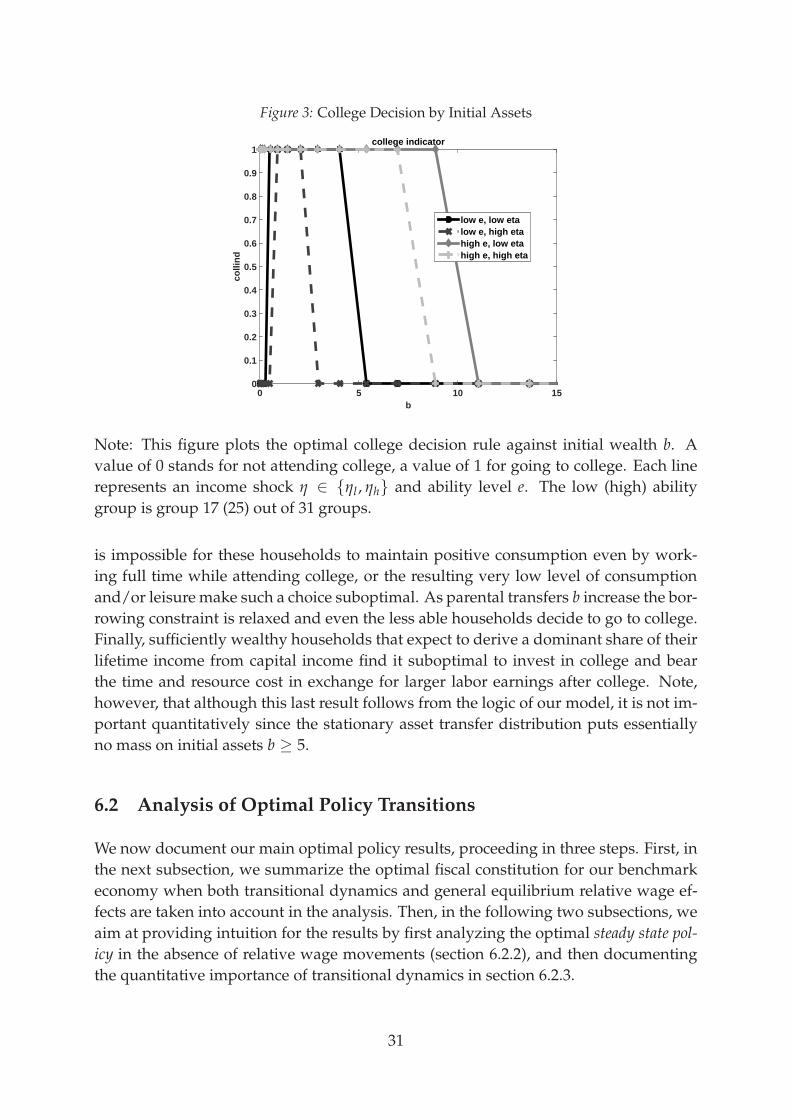
Figure 3: College Decision by Initial Assets

b0 5 10 15

colli

nd

0

0.1

0.2

0.3

0.4

0.5

0.6

0.7

0.8

0.9

1college indicator

low e, low etalow e, high etahigh e, low etahigh e, high eta

Note: This figure plots the optimal college decision rule against initial wealth b. A

value of 0 stands for not attending college, a value of 1 for going to college. Each line

represents an income shock η ∈ {ηl , ηh} and ability level e. The low (high) ability

group is group 17 (25) out of 31 groups.

is impossible for these households to maintain positive consumption even by work-

ing full time while attending college, or the resulting very low level of consumption

and/or leisure make such a choice suboptimal. As parental transfers b increase the bor-

rowing constraint is relaxed and even the less able households decide to go to college.

Finally, sufficiently wealthy households that expect to derive a dominant share of their

lifetime income from capital income find it suboptimal to invest in college and bear

the time and resource cost in exchange for larger labor earnings after college. Note,

however, that although this last result follows from the logic of our model, it is not im-

portant quantitatively since the stationary asset transfer distribution puts essentially

no mass on initial assets b ≥ 5.

6.2 Analysis of Optimal Policy Transitions

We now document our main optimal policy results, proceeding in three steps. First, in

the next subsection, we summarize the optimal fiscal constitution for our benchmark

economy when both transitional dynamics and general equilibrium relative wage ef-

fects are taken into account in the analysis. Then, in the following two subsections, we

aim at providing intuition for the results by first analyzing the optimal steady state pol-

icy in the absence of relative wage movements (section 6.2.2), and then documenting

the quantitative importance of transitional dynamics in section 6.2.3.

31

6.2.1 The Optimal Policies

Table 3 displays the optimal policy combinations, both for maximizing steady state and

transitional welfare.39 In addition, the table provides summary measures of aggregate

economic activity40 and inequality statistics for the initial steady state with status quo

policy (column 2), and the final state of the optimal policy induced transition (column

3). Column 4 shows the change in these variables between the initial and the final

steady state.41 Finally, columns 5 and 6 do the same, but for the optimal steady state

policy that ignores transitional dynamics and hence transitional welfare.42

The first five rows of table 3 display the fiscal constitution in the economy, both in the

initial steady state as well as in the social optimum. Recall that τl is the marginal labor

income tax rate, θ the public subsidy rate, Z = d YN is the size of the labor income tax

deduction and d measures the size of the deduction relative to income per capita. They

show that (see columns 3 and 4 of the table43), starting from the status quo, the opti-

mal policy transition is obtained by a significantly larger education subsidy of 150%

and a significantly less progressive tax system. The deduction d falls from 27% to 6%

of average income, and thus the optimal tax system, when combined with a generous

education subsidy, is not far away from a proportional labor income tax system. The

welfare gains from the optimal policy transition, relative to the status quo are substan-

tial, in the order of 3.5% of lifetime consumption.

In order to start understanding where these welfare gains emerge from we turn to the

remaining rows of table 3 and figure 4, which collects the transitional dynamics of key

macroeconomic aggregates induced by the optimal policy reform.

The upper left panel of figure 4 displays both the share of the youngest cohort going

to college as well as the overall fraction of the population. It shows that the increase

in the college subsidy and the reduction in marginal (and average) tax rates for high

income earners induces a college boom on impact. The share of the youngest cohort

completing college rises from 44% in the initial steady state to about 67% in the first

39 In order to meaningfully compare the optimal steady state policies and the optimal transition poli-

cies we adopt the same type of welfare criterion when maximizing steady state welfare as when

maximizing transitional welfare: the integral of lifetime utilities, weighted by the cross-sectional

distribution of state variables in the intitial steady state. In contrast to maximizing expected utility

of a newborn household (as often done in the literature, see e.g. Conesa et al., 2009), this welfare

measure places positive weight on older households even in the steady state.

40 All variables are denoted in per capita terms.

41 For variables that are already in % units we report the percentage point changes. For the Gini coeffi-

cients we simply report the point changes.

42 When characterizing optimal steady state policies we hold constant the government debt to GDP

ratio at its initial steady state level.

43 We will return to the optimal steady state results in columns 5 and 6 below.

32

Table 3: Benchmark Results: Optimal Policies and Macroeconomic Aggregates in the Long Run

Trans. Dynamics Steady State

Var. Status Quo Opt. Pol. Change Opt. Pol. Change

τl 27.55% 21.9% -5.69%p 26.03% -1.53%p

d 27.1% 6% -21.1%p 10% -17.1%p

θ 38.8% 150% 111.2%p 200% 161.2%p

Z 0.0714 0.0171 -76.05% 0.0281 -60.57%

τl · Z 0.0197 0.0037 -80.98% 0.0073 -62.76%

Y/N 0.2633 0.2847 8.15% 0.2813 6.85%

B/Y 60.16% 79.81% 19.65%p 60.16% 0%p

K/N 0.1731 0.1899 9.73% 0.1866 7.8%

L/N 2.2097 2.3782 7.63% 2.3508 6.39%

K/L 0.1097 0.1118 1.95% 0.1111 1.33%

w 0.1118 0.1123 0.49% 0.1122 0.44%wcwn

0.3801 0.2946 -22.49% 0.2732 -28.12%

r 5.37% 5.26% -0.11%p 5.27% -0.09%p

hours 0.326 0.3392 1.32% 0.3329 0.7%

C/N 0.1628 0.1795 10.28% 0.1731 6.32%

Trans/Assets 1.15% 1.01% -0.15%p 0.78% -0.37%p

college share 43.89% 54.37% 10.48%p 58.57% 14.68%p

Gini(c) 0.235 0.2078 -2.72 p 0.1996 -3.54 p

Gini(h) 0.12 0.1266 0.66 p 0.1243 0.43 p

Gini(a) 0.5558 0.5369 -1.89 p 0.5493 -0.65 p

CEV 3.4652% 2.7569%

Note: This table summarizes optimal policies and the long-run change in macroeco-

nomic aggregates, distributions and welfare for ρ = 0.285 (an elasticity of substitution

between unskilled and skilled labor of 1.4).

period of the policy transition.44

The second observation we make from the upper left panel is that the share of college

bound youngsters is falling over time. The reason for this reduction is displayed in

44 We also observe a further discrete upward jump in the share of the newborn cohort attending college

30 years after the initial policy reform. The distribution of ability of children is partially determined

by the persistence of innate ability, but also impacted by parental education. The boost of college

attendance on impact generates more highly educated parents thirty years later, and thus a more

favorable college ability distribution which in turn makes a higher share of children attend college

themselves. Further, but smaller, echo effects are observed for later generations.

33

Figure 4: Evolution of Macroeconomic Aggregates: Imperfect Substitutes

year0 50 100 150

1

1.2

1.4

1.6

1.8Fraction of (i) Students, (ii) Pop with College Degree

Φ(1,s=c)Φ(s=c)

year0 50 100 150

1

1.05

1.1

1.15

1.2Output, Capital, Labor

Y/NK/NL/N

year0 50 100 150

1

1.05

1.1

1.15

1.2Consumption, Hours

C/NH/WN

year0 50 100 150

1

1.2

1.4

1.6

1.8

2Debt

B/NB/Y

Note: this figure plots the transition paths of key macroeconomic aggregates aginst

time. The elasticity of substitution between unskilled and skilled labor is 1.4 (ρ =

0.285)

figure 5 which shows wages of college and non-college households relative to their

initial steady state levels. From the figure it is clear that the college wage premium

decreases substantially over time.45 Consequently the college boom lessens over time,

although the share of young cohorts going to college remains about 23% (or about

10.5% points) above its initial steady state level. As a consequence, as we will show in

sections 6.2.2 and 6.2.3, the skill distribution improves much less pronouncedly in the

economy with general equilibrium relative wage effects, compared to the economy in

which this effect is absent.

Third, whereas the share of the youngest cohort going to college increases immediately

by close to 60% on policy impact, it takes approximately two generations (roughly 60

years) until the overall skill distribution has reached a level close to its new steady state

value. It is this sluggish dynamics of the skill and thus labor productivity distribution

that a restriction to a long-run steady state policy analysis would miss completely.

45 Also note that, at least in the long-run, the overall wage level per efficiency unit of labor increases

moderately, see table 3. In consequence, absolute wages of the unskilled increase and this increases

is stronger than the fall of wages of the skilled.

34

Figure 5: Wages of College and Non-College Households: Imperfect Substitutes

time0 50 100 150

0.85

0.9

0.95

1

1.05

1.1

1.15

1.2Wages of College / Non-College Workers [Index: t

0=1]

Wages(c)Wages(n)

Note: this figure plots the transition paths of (average) wages for college-educated and

unskilled workers aginst time. The elasticity of substitution between unskilled and

skilled labor is 1.4 (ρ = 0.285)

The trends in educational attainment and thus average labor productivity are reflected

in aggregate output and consumption, as figure 4 and table 3 show. First, focusing

on the long run steady state, the optimal policy reform has a strong long-run positive

effect on output and consumption per capita (8% and 10.3% in table 3), despite the fact

that hours worked only move moderately (by 1.3% points) in response to the lower

marginal labor income taxes. Nevertheless labor efficiency units per person LN increase

drastically (by 7.7%) in the new, relative to the old steady state, on account of a more

skilled workforce.

However, as discussed above, the skill distribution evolves slowly. The upper right

and the lower left panel of figure 6 show the corollary of this result: as the skill dis-

tribution improves only slowly and more and more on average more skilled cohorts

enter the labor force over time, effective labor units supplied and output per capita

(upper right panel) increase slowly along the transition as well. The lower right panel

documents the same for consumption, and also shows that average hours worked in-

crease on impact by about 3% (1.3% points) because of the decline in the marginal tax

rate τl. This is true despite the fact that a larger share of the youngest age cohort now

goes to college and thus withdraws temporarily from the labor force.46

Finally, the lower right panel of figure 6 displays the evolution of government debt

per capita and the debt-to-output ratio. Given the tax and education policy and the

46 College students can and do work while studying, but the hours they supply are quantitatively

minor.

35

initial debt level the sequence of government debt is determined from the sequence of

period government budget constraints. The government finds it optimal (through the

setting of τl , θ, d), to smooth the transitional costs of building up a higher human capital

stock (i.e., high education policy costs and relatively lax revenues due to low—relative

to the final steady state—economic activity) by borrowing along the transition. As a

consequence the debt to output ratio increases from 60% to 80% (an increase of about

20% percentage points, or 33%) along the transition. Debt per capita is increasing more

strongly than that since GDP is also increasing along the transition, although not at the

same speed as debt itself, which explains the increase in the debt to GDP ratio.

On the distributional side, consumption and wealth inequality fall despite the reduc-

tion in the labor income tax progressivity. This is mainly due to the fact that in the final

steady state there are significantly less consumption- and wealth poor unskilled house-

holds. Furthermore, the college wage premium shrinks significantly in response to the

policy reform, further aiding the decline in consumption inequality. Overall, and to

summarize, the policy reform increases educational attainments, raise output and con-

sumption per capita significantly both in the short and in the long run on account of a

more productive workforce and at the same time reduces consumption inequality on

account of a narrowing college wage premium, despite the fact that the tax system has

become less redistributive.47 In the next subsections we document the importance of

the general equilibrium wage effects as well as an explicit consideration of the transi-

tional dynamics for this finding.

6.2.2 The Importance of General Equilibrium Relative Wage Effects

In table 4 we summarize the optimal policy reforms and associated aggregate and dis-

tributional consequences in an economy where skilled and unskilled labor are perfect

substitutes but all other model parameters remain unchanged.48

Comparing first the optimal steady state policies (column 5 and 6 in both tables 3 and

4) between the benchmark economy and the perfect substitutes case reveals the im-

portance of the general equilibrium wage effects for optimal policy design. Whereas

the optimal education subsidy is similarly large in both cases (and substantially larger

than in the initial status quo) the degree of tax progressivity differs fundamentally. In

the benchmark economy where redistribution across different ability e types and thus

across eduction groups can be achieved through the general equilibrium wage effects

induced by the education subsidies, a strongly progressive tax system is not desirable

even in the steady state: d = 10% is optimal, relative to the benchmark of d = 27%.

47 Hours worked increase slightly and hours (and thus leisure) inequality rises somewhat, but both

effects are quantitatively rather modest.

48 Recall that appendix C.2 demonstrates that by simply scaling the aggregate TFP parameter we can

insure that this version of the model attains the same aggregates in the initial steady state as the

benchmark economy

36

If education policies stimulating college attendance do not affect the college wage pre-

mium as in the perfect substitutes case, instead a strongly progressive tax system with

a deduction worth 31% of average income (and thus more progressive than the status

quo) is optimal when the government is maximizing steady state welfare.

Table 4: Optimal Policies and Macroeconomic Aggregates in the Long Run: Perfect Substitutes

Trans. Dynamics Steady State

Var. Status Quo Opt. Pol. Change Opt. Pol. Change

τl 27.55% 22.9% -4.68%p 36.98% 9.43%p

d 27.1% 10% -17.1%p 31% 3.9%p

θ 38.8% 120% 81.2%p 170% 131.2%p

Z 0.0714 0.0303 -57.56% 0.0866 21.38%

τl · Z 0.0197 0.0069 -64.75% 0.032 62.94%

Y/N 0.2633 0.3032 15.15% 0.2794 6.12%

B/Y 60.16% 96.95% 36.79%p 60.16% 0%p

K/N 0.1731 0.1951 12.74% 0.1781 2.92%

L/N 0.4532 0.5259 16.06% 0.4882 7.73%

K/L 0.5346 0.5194 -2.86% 0.5108 -4.47%

w 0.5449 0.5407 -0.78% 0.5368 -1.5%wcwn

1 1 0% 1 0%

r 5.37% 5.54% 0.17%p 5.7% 0.33%p

hours 0.326 0.3287 0.27% 0.2985 -2.75%

C/N 0.1628 0.1934 18.82% 0.1717 5.47%

Trans/Assets 1.15% 1.39% 0.23%p 0.78% -0.37%p

college share 43.89% 75.79% 31.9%p 82.07% 38.18%p

Gini(c) 0.235 0.2186 -1.64 p 0.1987 -3.62 p

Gini(h) 0.12 0.1283 0.83 p 0.1176 -0.24 p

Gini(a) 0.5558 0.5203 -3.55 p 0.5336 -2.22 p

CEV 1.6565% 2.6126%

Note: This table summarizes optimal policies and the long-run change in macroeco-

nomic aggregates, distributions and welfare for ρ = 1 (in which case unskilled and

skilled labor are perfect substitutes in production).

From table 4) we observe that the steady state optimal policy change reduces hours

worked in the steady state substantially (by 2.75% points, or 8.4%). However, absent

the reduction in the college wage premium the education boom is so massive that labor

input as well as output and consumption per capita rise substantially. The reduction

in consumption inequality and the welfare gains are similar between the steady states

in the imperfect substitutes case and the perfect substitutes case, but they are achieved

37

with different tools: in the latter case, since relative wages don’t move by construction,

redistribution has to be achieved via the income tax code, as a deduction of d = 31%

(relative to d = 10% in the benchmark) shows. This in turn has severe consequences

for the importance of the transitional dynamics in optimal policy design, as the next

subsection will demonstrate.

6.2.3 Transitional Dynamics

Figure 6: Evolution of Macroeconomic Aggregates: Perfect Substitutes

year0 50 100 150

1

1.2

1.4

1.6

1.8Fraction of (i) Students, (ii) Pop with College Degree

Φ(1,s=c)Φ(s=c)

year0 50 100 150

1

1.05

1.1

1.15

1.2Output, Capital, Labor

Y/NK/NL/N

year0 50 100 150

1

1.05

1.1

1.15

1.2Consumption, Hours

C/NH/WN

year0 50 100 150

1

1.2

1.4

1.6

1.8

2Debt

B/NB/Y

Note: this figure plots the transition paths of key macroeconomic aggregates aginst

time. Unskilled and skilled labor are prefect substitutes (ρ = 1)

As already discussed in the benchmark case, it takes time (and resources) to build up a

more skilled workforce, suggesting that an explicit consideration of the transition path

is important. Comparing the optimal policy transition and the steady state optimal

policy (columns 3 and 5 of table 4) strongly reinforces this point. Explicitly taking into

account the transitional costs, the optimal tax code should become less, not more pro-

gressive. This raises two questions, a) why is there such a divergence between steady

state optimal and dynamically optimal policies? and b) why doesn’t this divergence

show up in the benchmark version of the model (compare columns 3 and 5 of table 3)?

The answer to the first question is contained in figures 6, displaying the evolution

38

of macroeconomic aggregates in the perfect substitution case under the transition-

optimal policy and showing monotonically increasing aggregate consumption, and

figure 7 which shows the transition path for consumption for different policy com-

binations. We see in figure 7 how the economy goes through a recession if the decrease

of taxes and the reduction of the tax deduction would not have taken place when the

education subsidy is increased (d = 0.27, θ = 1.2). As households are drawn from

the labor market into college, the economy experiences a transitional decline in out-

put and per capita consumption. The figure also shows the outcome along the transi-

tion if the government would implement the optimal steady state policy combination

(d = 0.31, θ = 1.7). In this case the recession is even more severe because the subsidy

is substantially higher and so are marginal labor income taxes and the tax deduction.49

Figure 7: Evolution of Per-Capita Consumption: Perfect Substitutes

time0 50 100 150

C/N

t/C/N

0

0.85

0.9

0.95

1

1.05

1.1

1.15

1.2C/N: Index [t

0=1]

d=0.31, theta=1.7d=0.27, theta=1.2d=0.1, theta=1.2

Note: this figure plots the transition paths of per capita consumption under different

policy configurations. The elasticity of substitution between unskilled and skilled labor

is 1.4 (ρ = 0.285).

Table 5 summarizes the associated welfare consequences from the policy reform. With

the increase of the tax subsidy alone, there are still welfare gains, but they are much

smaller than in the optimum. An implementation of the optimal steady state policy in-

stead leads to substantial welfare losses along the transition. These findings represent

our first main result perhaps most clearly: an explicit consideration of the transition

path when conducting a normative welfare analysis of education and tax policies can

change even the qualitative prescriptions for optimal fiscal policy dramatically.

49 Interestingly, the long-run increase of per capita consumption is smaller than in the steady state

comparison. Taking the transition into account when implementing the optimal steady state policy

leads to a long-run increase of per capita consumption by only about 2% whereas the last column of

table 4 shows an increase of about 5%.

39

Table 5: Welfare Consequences for Different Policy Combinations: Perfect Substitutes

d = 0.1, θ = 1.2 d = 0.27, θ = 1.2 d = 0.31, θ = 1.7

CEV 1.6565% 0.0981% -2.8027%

Note: This table displays the welfare gains, relative to the status quo, from transitions

induced by different policy configurations in the perfect substitution case.

This finding raises the second question: why doesn’t the same logic apply also to the

benchmark economy, where, as columns 3 and 5 of table 3) show, there is no strong

divergence between steady state and transition-optimal policies. In the next section we

argue that the answer lies in the fact that the general equilibrium wage effects allow the

government to achieve effective redistribution through education subsidies. Therefore

a high degree of tax progressivity (as embedded in a high deduction d) is not required

to achieve a less dispersed consumption distribution even in the steady state.

6.2.4 Progressive Income Taxation and Education Subsidies: Complements or Sub-

stitutes?

In this subsection we stress the importance of the general equilibrium wage response

to fiscal policy and explore its role further. As one summary measure, recall that the

welfare gain of switching to the optimal policy (d = 0.06, θ = 1.5) in the benchmark

economy was 3.5% (see column 4, last row in table 3). In comparison, the welfare gain

of this same policy reform in the economy with perfect substitutes (and thus absent

general equilibrium wage effects) is only 1.61%, close to the gain of 1.66% from the

optimal reform in this economy (see column 4, last row in table 4). Thus the general

equilibrium response, especially the reduction of the college wage premium, is very

important for the welfare assessment of the optimal policy.

In the simple model in the appendix we demonstrate how progressive taxes and edu-

cation subsidies can be complementary second best policies in a world where private

insurance is imperfect, and thus public insurance is potentially beneficial but distorts

human capital accumulation decisions, with education subsidies mitigating this distor-

tions. This model (and indeed the quantitative model with perfect substitutability of

labor) abstracted from the general equilibrium relative wage effects induced by these

policies which curbs the effectiveness of education subsidies for encouraging college

attendance. With the two types of labor being imperfect substitutes, the education pol-

icy now has indirect beneficial redistributive effects, by reducing the average wage gap

between skilled and unskilled workers, and thus might potentially be a substitute for

redistributive tax policies in general equilibrium.

To explore this theme further we compute optimal policies along one policy dimension,

holding the other dimension constant. We restrict ourselves to steady states to make

40

our points most clearly. Table 6 presents results for the perfect substitutes economy

in the left part which is easiest to interpret. The first column restates findings already

familiar from table 4. The next two columns document results for constrained-optimal

policies when one instrument (either the education subsidy θ or the size of the deduc-

tion d is held constant. The univariate optimization over d delivers the same optimal

degree of tax progressivity according to this measure (d = 0.31). However, compar-

ing the alternative measures for the progressivity of the income tax code, Z as well

as τl · Z, for the full optimum (column 2) with the constrained optimum (column 4)

where we hold θ constant, we observe the complementarity of policy instruments also

documented in the simple model in the Appendix in table 8 and stressed by Bovenberg

and Jacobs (2005). When θ is fixed at its status quo value of θ = 38.8%, which is lower

than the full steady state optimum of θ = 170%, the constrained optimal effective tax

deduction (as measured either by Z or τlZ) is lower as well.

Table 6: Final Steady State: Decomposition

Perfect Substitutes ρ = 1 Imperfect Substitutes ρ = 0.28

Var. Baseline Const. d Const. θ Baseline Const. d Const. θ

τl 36.9% 35.0% 29.3% 26.0% 32.5% 29.3%

d 31% 27.1% 31% 10% 27.1% 31%

θ 170% 175% 38.8% 200% 175% 38.8%

Z 0.086 0.077 0.08 0.028 0.071 0.080

τl · Z 0.032 0.027 0.023 0.007 0.023 0.023

CEV 2.612% 2.508% 0.167% 2.756% 2.413% 0.130%

Note: This table displays the steady state welfare gains for different policy configura-

tions.

Table 6 also shows that most of the (steady state) welfare gains stem from an adjust-

ment of the education subsidy: the best steady state policy reform brings welfare gains

of 2.6% of lifetime consumption, and only adjusting the education subsidy generates

almost the same welfare gains of 2.5% (since the optimal tax progressivity is close to

the status quo), whereas adjusting the progressivity of the labor income tax code alone

yields only gains of 0.17% (since the optimal education subsidy is much larger than the

status quo). Of course, absent general equilibrium wage effects the education policy

is very effective in stimulating college attendance and thus labor productivity in the

long run; along the transition this policy is not nearly as beneficial, which also explains

why the transitional welfare gains are lower than the long-run benefits, compare the

last row of columns 4 and 6 of table 4.

The right part of Table 6 repeats the same decomposition exercise for the imperfect sub-

stitutes case with general equilibrium wage effects. Interestingly, we observe that the

univariate optima favor a higher degree of tax progressivity and education subsidies,

41

just as for the case with perfect substitutes. However, once both policy instruments are

in operation, the two instruments become substitutes: in the unconstrained optimum,

the degree of education subsidies is higher than in the univariate optimum and tax

progressivity decreases. Now the additional effect of a decrease of the college wage

premium allows the government to achieve a more equal consumption distribution

(at least across college- vs. non-college households) either through college education

subsidies or progressive income taxes. Also, in this case transitional welfare gains are

larger than long-run welfare gains since the GE wage reactions only play out in the

long-run and reduce college attendance.

We conclude this section by summarizing our second main finding: whether the two

policies complement each other or become substitutes in providing redistribution cru-

cially depends on the importance of general equilibrium effects. Since we find the em-

pirical evidence for imperfect substitutability of skilled and unskilled labor compelling

we conclude that the case for education subsidies and progressive labor income taxes

being substitutable policies is strong.

6.3 Sensitivity Analysis

6.3.1 Restrictions on the Policy Space

In order to render our analysis computationally feasible we studied simple policy in-

struments and restricted them to be constant along the transition path. In this subsec-

tion we explore the question whether our results are driven by these restrictions.

Quantitatively, the most prominent finding is the optimality of large education sub-

sidies. These subsidies transfer resources to young households for going to college.

Here we briefly ask whether this policy is welfare improving simply because it pro-

vides intergenerational redistribution towards young, potentially credit-constrained

households. If this were the case, then unconditional transfers that are not contingent

on college attendance should lead to similar or even larger welfare gains. Restricting

ourselves to steady-state optimal policies50 we find an optimal policy combination of

d = 10% and θ = 160%, with welfare gains of 1% instead of 2.76%. That is, substantial

lump-sum transfers to the young remain optimal, but they are less effective in improv-

ing social welfare since they are not targeted at college attendees which stimulates less

college attendance.51 The share of college youngsters increases to 49% only instead

of 58.6%. This reduces the college wage premium by less (it falls only by 14.4% in-

stead of 28.1%) which is the key source of the welfare gain according to our baseline

50 Which in any case do not deviate much from the transition-optimal policies in the benchmark econ-

omy with imperfect substitutability of labor.

51 The optimal education-contingent policy makes borrowing constraints irrelevant for the education

allocation, as the share of college attendants is invariant to the tightness φ of the borrowing constraint

if education subsidies are set to θ = 150%

42

results. We conclude that making transfers to the young less education-targeted is not

beneficial.52

Second, we study whether the government forgoes important welfare gains by not

phasing in the policy reforms more slowly, permitting time-varying fiscal and educa-

tion policies. To do so we now consider transitional policies of the form

τl,t = e−ω(t−1)τl,0 + (1 − e−ω(t−1))τl,T

θt = e−ω(t−1)θ0 + (1 − e−ω(t−1))θT

dt = e−ω(t−1)d0 + (1 − e−ω(t−1))dT

where (τl,0, θ0, d0) is the calibrated policy in the initial steady state and (τl,T, θT, dT) is

an arbitrary time constant new policy, and ω ∈ [0, ∞) is a parameter that governs the

speed of adjustment. If ω = ∞ then adjustment is immediate; this is the assumption

we make in the paper. The smaller is ω, the more gradual the new policy is being

introduced. Using this structure we ask two related questions:

1. Is it optimal to more gradually introduce the policy we found to be optimal along

the transition? To answer this question we take (τl,T, θT, dT) = (τ∗l , θ∗, d∗) and

maximize social welfare with respect to ω. The answer we found is, to a very

good approximation (ω = 4), there is no benefit from introducing the optimal

policy more gradually. In this (limited) sense results are robust towards permit-

ting time variation in the policy instruments.

2. Is the suboptimality of the policy that maximizes steady state welfare along the

transition due to the fact that it is introduced too rapidly? We now take the

steady-state optimal policy (τl,T, θT, dT) = (τSSl , θSS, dSS) and again maximize

social welfare with respect to ω. Now the answer is, yes, the steady state optimal

policy leads to larger welfare gains along the transition if it is introduced more

slowly and phased in over a time interval of about 16 years.53

6.3.2 Alternative Parameterizations

Our model contains many parameters that determine the quantitative magnitudes of

the optimal policies. We have documented the importance of the degree of substi-

tutability of skilled and unskilled labor for the results. Our choice of substitution

elasticity for the case with imperfect substitutes was 1.4, based on the conventional

52 On the other hand we need to acknowledge that policies that make education subsidies parental

income- or wealth specific or condition them (if feasible) directly on student ability are likely to

do even better, since our policy subsidizes even students that would have gone to college in any

case. Findeisen and Sachs (2015), for example, find that the Pareto optimal policy in their model is

characterized by income-contingent student loans.

53 Of course, the transition-optimal policy still dominates the slowly introduced steady state policy

43

estimates by Katz and Murphy (1992) or Borjas (2003). According to Card (2009) an

alternative reasonable estimate is 3.33, i.e., a value of ρ of 0.7. We recompute the opti-

mum with such an alternative calibration for the steady state comparison with imper-

fect substitutes. We find that the optimal education subsidy θ falls from 200% to 190%,

and tax progressivity as measured by d goes up from 10% to 16%. The optimal labor in-

come tax rate is 28.8% instead of 26%. Results are thus in between the benchmark and

perfect substitutes case, but quantitatively (and qualitatively) closer to the benchmark.

One key endogenous decision is the education decision, which is shaped by public ed-

ucation policies and private intergenerational transfers. The size of the latter is in turn

determined by υ, the weight of children’s lifetime utility in parental welfare. We cali-

brated υ so that the magnitude of intergenerational transfers in the model is consistent

with SCF data in the 1980’s. We now investigate whether the optimal large size of pub-

lic transfers tied to education that we found is sensitive to the magnitude of private

transfers induced by a larger υ. We increase υ from 0.48 to 0.6 (and recalibrate all other

parameters), inducing inter-vivos transfers to rise by roughly one-third (from 1.1% to

1.6% of GDP) in the benchmark economy. Likewise total intergenerational transfers,

including accidental bequests, increase from 1.7% to 2.1% of GDP. Focusing on steady

state optima with imperfect substitutes the new optimum now features a lower degree

of tax progressivity (d = 8% instead of d = 10%) and a higher degree of education

subsidies (θ = 220% instead of θ = 200%) as well as a slightly lower optimal labor

income tax rate (τl = 25.9% instead of τl = 26%). Welfare gains increase to 3.62% (up

from 2.76%).54

7 Conclusions

In this paper we characterized the optimal mix of progressive income taxes and educa-

tion subsidies and argued that a large education subsidy and a moderately progressive

labor income tax and constitute part of the optimal fiscal constitution once household

college attendance decisions are endogenous and transitional dynamics are modeled

explicitly. The latter aspect (transitional dynamics) can have a crucial impact on the

optimal policy design, as the case of perfect substitutes indicates. Given the important

differences between steady state optimal and transition-optimal policy it is conceiv-

able, in fact likely, that policies that are time-varying over the transition provide further

welfare gains.55

In our thought experiment we also took the tax on capital income as exogenously

54 Evaluating welfare with the calibrated value of υ of 0.48 gives welfare gains of 3.0%, hence a large

part of the increase in welfare is due to the change in the social welfare function caused by recali-

brating υ.

55 Because of the high dimensionality of the policy space these fully time-varying might be hard to

characterize numerically for the near future, however.

44

given. Future work will need to determine whether our policy conclusions, especially

the high subsidy rates for human capital, remain robust once the government chooses

not only the progressivity of the labor income tax, but also the optimal mix between

capital and labor income taxes.

Finally we determined the optimal tax policy as one which maximizes Utilitarian so-

cial welfare among households currently alive.56 We also documented that both policy

instruments are potentially effective in generating more equally distributed consump-

tion and lifetime welfare. We leave for future work a detailed analysis which elements

of our optimal fiscal constitution remains intact if social preferences for insurance and

redistribution deviate from the Utilitarian benchmark we have analyzed here.

56 Although Utilitarian social welfare is commonly used in the literature, it is of course but one choice

for the social welfare function. For alternative criteria and their merits, see, e.g., Weinzierl (2012) or

Saez and Stantcheva (2013).

45

References

[1] Abbott, B., G. Gallipoli, C. Meghir and G. Violante (2013), “Education Policy and

Intergenerational Transfers in Equilibrium,” Working Paper.

[2] Aiyagari, R. (1994), “Uninsured Idiosyncratic Risk and Aggregate Saving,” Quar-

terly Journal of Economics, 109(3): 659-684.

[3] Alvarez, Y., J. Burbidge, T. Farrell, and L. Palmer (1992), “Optimal Taxation in a

Life-Cycle Model,” Canadian Journal of Economics, 25, 111-122.

[4] Auerbach, A. and L. Kotlikoff (1987), Dynamic Fiscal Policy, Cambridge University

Press.

[5] Bakis, O., B. Kaymak and M. Poschke (2014), “Transitional Dynamics and the Op-

timal Progressivity of Income Redistribution,”Review of Economic Dynamics, forth-

coming.

[6] Benabou, R. (2002), “Tax and Education Policy in a Heterogeneous-Agent Econ-

omy: What Levels of Redistribution Maximize Growth and Efficiency?" Economet-

rica, 70, 481-517.

[7] Bewley, T. (1986), “Stationary Monetary Equilibrium with a Continuum of Inde-

pendently Fluctuating Consumers,” in Werner Hildenbrand and Andreu Mas-

Colell (eds.) Contributions to Mathematical Economics in Honor of Gerard Debreu,

North-Holland, 79-102.

[8] Bohacek, R. and M. Kapicka (2008), “Optimal Human Capital Policies,” Journal of

Monetary Economics, 55, 1-16.

[9] Bohacek, R. and M. Kapicka (2012), “A Quantitative Analysis of Educational Re-

forms in a Dynastic Framework,” Manuscript, University of California Santa Bar-

bara.

[10] Borjas, G. (2003), “The Labor Demand Curve is Downward Sloping: Reexamining

the Impact of Immigration on the Labor Market,” Quarterly Journal of Economics,

118, 1335-1374

[11] Bovenberg, L., and B. Jacobs (2005), “Redistribution and Education Subsidies are

Siamese Twins,” Journal of Public Economics, 89, 2005–2035.

[12] Brown, M., M. Mazzocco, J. Scholz and A. Seshadri (2006), “Tied Transfers,” Work-

ing Paper.

[13] Card, D. (2009), “Immigration and Inequality,” American Economic Review, 99(2),

1–21.

46

[14] Castañeda, A., J. Díaz-Giménez and V. Ríos-Rull (1999), “Earnings and Wealth In-

equality and Income Taxation: Quantifying the Trade-offs of Switching to a Pro-

portional Income Tax in the U.S.” Working Paper.

[15] Caucutt, E., K. Kumar and S. Imrohoroglu (2006), “Does the Progressivity of In-

come Taxes Matter for Human Capital and Growth?,” Journal of Public Economic

Theory, 8, 95-118.

[16] Chamley, C. (1986), “Optimal Taxation of Capital Income in General Equilibrium

with Infinite Lives,” Econometrica, 54, 607-622.

[17] Chari, V. V., and P. Kehoe (1999), “Optimal Fiscal and Monetary Policy,” In Hand-

book of Macroeconomics, ed. John B. Taylor and Michael Woodford, 1671-1745. Am-

sterdam: North Holland.

[18] Chari, V. V., and P. Kehoe (2006), “Modern Macroeconomics in Practice: How

Theory Is Shaping Policy,” Journal of Economic Perspectives, 20, 3-28.

[19] Conesa, J. and D. Krueger (2006), “On the Optimal Progressivity of the Income

Tax Code,” Journal of Monetary Economics, 53, 1425-1450.

[20] Conesa, J., S. Kitao and D. Krueger (2009), “Taxing Capital: Not a Bad Idea after

All!,” American Economic Review, Vol 99, 25-48.

[21] Cunha, F., J. Heckman, L. Lochner and D. Masterov (2006), Interpreting the Ev-

idence on Life Cycle Skill Formation, Handbook of the Economics of Education,

Vol. 1, 697-812.

[22] Dynarski, S. (2003), “Does Aid Matter? Measuring the Effect of Student Aid on

College Attendance and Completion, ” American Economic Review, 93, 279-288.

[23] Domeij, D. and J. Heathcote (2004), On the Distributional Effects of Reducing Cap-

ital Taxes, International Economic Review, 45, 523-554.

[24] Erosa, A. and M. Gervais (2002), “Optimal Taxation in Life Cycle Economies,”

Journal of Economic Theory, 105, 338-369.

[25] Fehr, H. and F. Kindermann (2015), “Taxing Capital along the Transition - Not a

Bad Idea After All?,” Journal of Economic Dynamics and Control, 51, 64-77.

[26] Fernandez-Villaverde, J. and D. Krueger (2011), “Consumption and Saving over

the Life Cycle: How Important are Consumer Durables? (with J. Fernandez-

Villaverde), ”Macroeconomic Dynamics, 15, 725-770.

[27] Findeisen, S. and D. Sachs (2013), “Education and Optimal Dynamic Taxation:

The Role of Income-Contingent Student Loans,” Working Paper.

[28] Findeisen, S. and D. Sachs (2014), “Designing Efficient College and Tax Policies,”

Working Paper.

47

[29] Fukushima, K. (2010), “Quantifying the Welfare Gains from Flexible Dynamic In-

come Tax Systems,” Working paper, University of Wisconsin.

[30] Garriga, C. (2003), “Optimal Fiscal Policy in Overlapping Generations Models,”

Working Paper.

[31] Gale, W. and J. Scholz (1994), “Intergenerational Transfers and the Accumulation

of Wealth,” Journal of Economic Perspectives, American Economic Association, 8, 145-

60.

[32] Gervais, M. (2012), “On the Optimality of Age-Dependent Taxes and the Progres-

sive U.S. Tax System,” Journal of Economic Dynamics and Control, 36, 682-691.

[33] Greenwood, J, Z. Hercowitz, and G. Hoffman (1988), “Investment, Capacity Uti-

lization, and the Real Business Cycle,” American Economic Review, 78, 402-417.

[34] Guvenen, F., B. Kuruscu and S. Ozkan (2014), “Taxation of Human Capital and

Wage Inequality: A Cross-Country Analysis,” Review of Economic Studies,

81, 818-850.

[35] Heckman, J., L. Lochner and C. Taber (1998), “Tax Policy and Human-Capital

Formation,” American Economic Review, 88, 293-297.

[36] Heckman, J., L. Lochner and C. Taber (1999), “Human Capital Formation and

General Equilibrium Treatment Effects: A Study of Tax and Tuition Policy,” Fiscal

Studies, 20, 25-40.

[37] Heckman, J., L. Lochner and P. Todd (2006), “Earnings Functions, Rates of Re-

turn and Treatment Effects: The Mincer Equation and Beyond,” Handbook of the

Economics of Education, 307-458.

[38] Heathcote, J., F. Perri and G. Violante (2010), “Unequal We Stand: An Empirical

Analysis of Economic Inequality in the United States, 1967-2006,” Review of Eco-

nomic Dynamics, 13, 15-51

[39] Heathcote, J., S. Storesletten and G. Violante (2014), “Optimal Tax Progressivity:

An Analytical Framework,”Working paper.

[40] Holmlund, H., M. Lindahl and E. Plug (2011), The Causal Effect of Parents’

Schooling on Children’s Schooling: A Comparison of Estimation Methods,” Jour-

nal of Economic Literature, 49, 615-651.

[41] Holter, H. (2014), “Accounting for Cross-Country Differences in Intergenerational

Earnings Persistence: The Impact of Taxation and Public Education Expenditure,”

Working Paper.

[42] Hubbard, G. and K. Judd (1986), “Liquidity Constraints, Fiscal Policy, and Con-

sumption,” Brookings Papers on Economic Activity, 1986, 1-50.

48

[43] Huggett, M. (1993), “The Risk-Free Rate in Heterogeneous-Agent Incomplete-

Insurance Economies,” Journal of Economic Dynamics and Control, 17, 953-969.

[44] Huggett, M. (1997), “The One-Sector Growth Model with Idiosyncratic Shocks:

Steady States and Dynamics,” Journal of Monetary Economics, 39, 385-403.

[45] Ionescu, F. and N. Simpson (2014), “Credit Scores and College Investment: Impli-

cations for Student Loan Policies,” Working paper, Colgate University.

[46] Jacobs, B. and L. Bovenberg (2010), “Human Capital and Optimal Positive Taxa-

tion of Capital Income,” International Tax and Public Finance, 17, 451-478.

[47] Judd, K. (1985), “Redistributive Taxation in a Simple Perfect Foresight Model,”

Journal of Public Economics, 28, 59-83.

[48] Judd, K. and C. Su (2006), ”Optimal Income Taxation with Multidimensional Tax-

payer Types,” Working Paper.

[49] Kapicka, M. (2011), “The Dynamics of Optimal Taxation when Human Capital is

Endogenous,” Working Paper.

[50] Karabarbounis, M. (2012), “Heterogeneity in Labor Supply Elasticity and Optimal

Taxation,” Working Paper.

[51] Katz, L. and K. Murphy (1992), “Changes in Relative Wages, 1963-1987: Supply

and Demand Factors,” Quarterly Journal of Economics, 107, 35-78.

[52] Keane, M. and K. Wolpin (2001), “The Effect of Parental Transfers and Borrowing

Constraints on Educational Attainment,” International Economic Review, 42, 1051-

1103.

[53] Kindermann, F. (2012), “Welfare Effects of Privatizing Public Education When Hu-

man Capital Investments Are Risky,” Journal of Human Capital, 6, 87-123.

[54] Krueger, D. and A. Ludwig (2013), “Optimal Progressive Labor Income Taxation

and Education Subsidies When Education Decisions and Intergenerational Trans-

fers are Endogenous,” American Economic Review, 103, 496-501.

[55] Lochner, L. and A. Monge (2011), “Credit Constraints in Education,” forthcoming,

Annual Review of Economics.

[56] Ludwig, A., T. Schelkle and E. Vogel (2012), “Demographic Change, Human Cap-

ital and Welfare,” Review of Economic Dynamics, 15(1), 94-107.

[57] Mendoza, E., A. Razin and L. Tesar (1994), “Effective Tax Rates in Macroeco-

nomics: Cross-Country Estimates on Factor Income and Consumption,” Journal

of Monetary Economics, 34, 297-323.

49

[58] Mirrless, J. (1971), “An Exploration in the Theory of Optimum Income Taxation,”

Review of Economic Studies, 38, 175-208.

[59] Rothschild, C. and F. Scheuer (2013), “Redistributive Taxation in the Roy Model,”

Quarterly Journal of Economics, 128, 623-668.

[60] Saez, E. and S. Stantcheva (2013), “Optimal Tax Theory with Endogenous Social

Marginal Welfare Weights,” Working paper, UC Berkeley.

[61] Stiglitz, J. (1982), “Self-Selection and Pareto Efficient Taxation,” Journal of Public

Economics, 17, 213-230.

[62] Weinzierl, M. (2011), “The Surprising Power of Age-Dependent Taxes,” Review of

Economic Studies, 78, 1-29.

[63] Weinzierl, M. (2012) “The Promise of Positive Optimal Taxation: A Generalized

Theory Calibrated to Survey Evidence on Normative Preferences Explains Puz-

zling Features of Policy,” NBER Working Paper 18599.

[64] Winter, C. (2014) “Accounting for the Changing Role of Family Income in Deter-

mining College Entry,” The Scandinavian Journal of Economics,

116, 909-963

50

A Online Theoretical Appendix: The Simple Model

Here we present the simple model57 that allows us to make precise the intuition from

the introduction that with incomplete financial markets progressive labor income taxes

might be part of optimal fiscal policy because it implements a more equitable consump-

tion distribution than the laissez faire competitive equilibrium, but that it distorts both

the labor supply and the education decision. The latter distortion can be partially offset

by an education subsidy which then becomes part of an optimal policy mix as well.

Relative to the quantitative model used in the main part of the paper, the model an-

alyzed here abstracts from general equilibrium feedbacks and the two key sources of

dynamics in that model, endogenous capital accumulation and the intergenerational

transmission of talent and wealth.

A.1 The Environment

The economy lasts for one period and is populated by a continuum of measure one of

households that differ by ability e. The population distribution of e is uniform on the

unit interval, e ∼ U[0, 1]. Households value consumption and dislike labor according

to the utility function

log

(c − µ

l1+ 1

ψ

1 + 1ψ

). (16)

These Greenwood, Hercowitz and Huffman (1988) preferences rule out wealth effects

on labor supply (which greatly enhances the analytical tractability of the model), but

at the same time make utility strictly concave in consumption, which induces a redis-

tribution/insurance motive for a utilitarian social planner or government.

A household can either go to college or not. A household with ability e that has gone

to college produces (1+ pe)w units of consumption per unit of labor, whereas a house-

hold without a college degree has labor productivity w. Here w > 0 and p > 0 (the

college premium for the most able type) are fixed positive parameters. Going to col-

lege requires κw resources (but no time) where κ > 0 is a parameter.

A.2 Social Planner Problem

Prior to analyzing the competitive equilibrium without and with fiscal policy we es-

tablish, as a benchmark, how a social planner with utilitarian social welfare function

would allocate consumption and labor across the population. The social planner prob-

lem chooses consumption and labor supply c(e), l(e) for each type e ∈ [0, 1] as well as

57 The model builds on the analysis in Bovenberg and Jacobs (2005) and Jacobs and Bovenberg (2010),

but is tailored towards being a special case of the quantitative model studied in the main text.

51

the set I of types that are being sent to college to solve

maxc(e),l(e),I

∫log

(c(e)− µ

l(e)1+ 1

ψ

1 + 1ψ

)de

s.t∫

c(e)de + κw∫

e∈Ide =

∫

e/∈Iwl(e)de +

∫

e∈I(1 + pe)wl(e)de

The following proposition summarizes its solution, under the following

Assumption 3(

µψ(1+ψ)κwψ + 1

) 11+ψ

− 1

p< 1.

Proposition 4 Suppose assumption 3 is satisfied. Then the solution to the social planner prob-

lem is characterized by an ability threshold eSP such that all households with e ≥ eSP are sent

to college (and indexed with subscript c from now on) and the other households are not (and are

indexed by n). Labor allocations are given by

ln =

(w

µ

)ψ

for all e < eSP (17)

lc(e) =

((1 + pe)w

µ

)ψ

for all e ≥ eSP (18)

Consumption allocations are characterized by

c(e) = cn for all e < eSP

c(e) = cc(e) = cn + µlc(e)

1+ 1ψ

1 + 1ψ

− µl1+ 1

ψn

1 + 1ψ

for all e ≥ eSP

The optimal education threshold satisfies the first order condition

κw =w1+ψ

µψ (1 + ψ)

((1 + peSP)1+ψ − 1

)(19)

and is given in closed form as

eSP =

(µψ(1+ψ)κ

wψ + 1) 1

1+ψ− 1

p= eSP(κ, p, w, µ) (20)

Thus the larger is p, w and the smaller is κ, µ, the smaller is the education threshold and thus

the more households are sent to college.

52

Proof 5 The threshold property of set I follows from the fact that the cost of college is indepen-

dent of e and the productivity benefits pe of being college-educated are strictly increasing in e.

The other results are directly implied by the first order conditions (which in the case of the ed-

ucation threshold eSP involves applying Leibnitz’ rule to the resource constraint, after having

substituted in the optimal labor allocations). Assumption 3 assures that eSP ∈ (0, 1). Note

that this assumption is purely in terms of the structural parameters of the model and requires

that the college productivity premium p is sufficiently large, relative to the college cost κ, for

the ablest households indeed be sent to college. Note that if ψ = 0 and thus labor supply is

inelastic, then assumption 3 simplifies to p > κ, insuring that the ablest person goes to college

since the wage premium more than compensates for the resource cost for tuition.

Equation (19) has an intuitive interpretation. The social planner chooses the optimal

education threshold such that the cost κw of education for the marginal type eSP equals

the net additional resources this marginal type generates with a college education, rel-

ative to producing without having obtained a college education. The term on the right

hand side of (19) takes into account that college educated households work longer

hours (this explains the exponent 1 + ψ) and the fact that college-educated house-

holds are compensated for their longer hours with extra consumption which explains

the factor 1µψ(1+ψ)

. This latter property of optimal allocations follows from the non-

separability of consumption and labor in preferences (16).

For future comparison with equilibrium consumption allocations we state:

Corollary 6 The optimal consumption allocation satisfies cn < cc(eSP) and cc(e) is strictly

increasing in e for all e > eSP.

We depict the optimal consumption allocation in figure 8, together with two equilib-

rium allocations discussed in the next subsection.58

A.3 Competitive Equilibrium

Now we study the competitive equilibrium of this economy. To do so we first have to

specify the market structure and the government policies. Households participate in

two competitive markets, the goods market where they purchase consumption goods,

and the labor market where they earn a wage per unit of labor supplied that equals

their marginal product. In addition to choosing consumption and labor households

decide whether to incur the cost κw of going to college. The benefit of doing so is a

wage premium epw > 0. We denote by I(e) ∈ {0, 1} the college choice of household

type e, with I(e) = 1 if the household goes to college.

58 The specific parameter values that underly this figure are discussed below as well.

53

Figure 8: Optimal and Equilibrium Consumption Allocations

0 0.2 0.4 0.6 0.8 10.9

1

1.1

1.2

1.3

1.4

1.5Consumption Allocation

Co

nsu

mp

tio

n

Ability e

Social PlannerLaissez FaireRamsey Policy

Note: this figure plots the efficient and equilibrium consumption allocations in the

simple model against household ability e.

Financial markets, however, are assumed to be incomplete. Although there is no scope

for intertemporal trade, in principle households would like to trade insurance con-

tracts against the risk of being born as a low ability e type, prior to the realization

of that risk. It is the insurance against this idiosyncratic wage risk that we rule out

by assumption, and this fundamental market failure will induce a motive of insur-

ance/redistribution for the benevolent, utilitarian government in this economy.59

We assume that the benevolent, utilitarian government (which from now on we will

frequently refer to as the Ramsey government) has access to three fiscal policy instru-

ment, a flat labor income tax with tax rate τ, a lump sum transfer/tax d · w and a

proportional education subsidy with rate θ. Note that by permitting d < 0 we allow

the government to levy lump sum taxes; on the other hand it can also implement a

progressive labor income tax schedule by setting d, τ > 0. What we do not permit

are policies that make taxes or subsidies type-specific by conditioning τ, d, θ on type e.

Given these restrictions on the tax code we would not expect the government to be able

to implement the solution to the social planner problem as a competitive equilibrium

with fiscal policies.

59 What is insurance ex ante (prior to the realization) of the e draws, is redistribution among different e

types ex post.

54

A.3.1 Definition and Characterization of Equilibrium

Now consider the problem of a generic household e ∈ [0, 1]. Given a fiscal policy the

household’s problem reads as

maxl(e),c(e)≥0,I(e)∈{0,1}

log

(c(e)− µ

l(e)1+ 1

ψ

1 + 1ψ

)(21)

s.t.

c(e) = (1 − τ)(1 + I(e)pe)wl(e) + dw − κw(1 − θ)I(e) (22)

Definition 7 For a given fiscal policy (τ, d, θ) a competitive equilibrium are consumption,

labor and education allocations c(e), l(e), I(e) such that

1. For all e ∈ [0, 1], the choices c(e), l(e), I(e) solve the household maximization problem

(21).

2. The government budget constraint is satisfied:

dw + κwθ∫

{e:I(e)=1}de = τ

(w∫

{e:I(e)=0}l(e)de + w

∫

{e:I(e)=1}(1 + pe)l(e)de

)

3. The goods market clears

∫c(e)de + κw

∫

{e:I(e)=1}de = w

∫

{e:I(e)=0}l(e)de + w

∫

{e:I(e)=1}(1 + pe)l(e)de

We can completely characterize the competitive equilibrium, for a given fiscal policy.

We summarize the results in the following

Proposition 8 Given a policy (τ, d, θ), the optimal labor supply of households not going to

college is given by

ln(τ) =

((1 − τ)w

µ

)ψ

(23)

whereas the optimal labor supply of households with a college education is given by

lc(e; τ) =

((1 − τ)(1 + pe)w

µ

)ψ

. (24)

The corresponding consumption allocations read as

cn(τ, d) =[(1 − τ)w]1+ψ

µψ + dw (25)

cc(e; τ, d, θ) =[(1 − τ)w]1+ψ (1 + pe)1+ψ

µψ + dw − κw(1 − θ) (26)

55

There is a unique education threshold eCE such that all types with e ≥ eCE go to college and the

others don’t. This threshold satisfies

cn(τ, d)−µln(τ)

1+ 1ψ

1 + 1ψ

= cc(eCE; τ, d, θ)−

µlc(τ, eCE)1+ 1

ψ

1 + 1ψ

and is explicitly given by60

eCE =

((1−θ)µψ(1+ψ)κ(1−τ)1+ψwψ + 1

) 11+ψ

− 1

p= eCE(τ, θ; κ, p, w, µ) (27)

The threshold eCE is strictly decreasing (the share of households going to college is strictly

increasing) in θ, strictly increasing in τ and independent of d.

Proof 9 The equilibrium labor allocations follow directly from the first order conditions of the

household problem. The equilibrium consumption allocations are then implied by plugging

equilibrium labor supply into the household budget constraint (22). Thus lifetime utility con-

ditional on not going to college is given by

log

(cn(τ, d)−

µln(τ)1+ 1

ψ

1 + 1ψ

)

which is constant in ability e, and lifetime utility conditional on going to college reads as

log

(cc(e; τ, d, θ)−

µlc(τ, e)1+ 1

ψ

1 + 1ψ

)

which is strictly increasing in e. The threshold result for the education decision thus follows,

and the threshold itself is determined by the indifference between attending and not attending

college at the threshold.

A.3.2 Optimality of Equilibrium without Government Intervention?

In this subsection we show that the unregulated competitive equilibrium displays an

optimal (in the sense of solving the social planner problem) labor and education allo-

cation and thus optimal production. However, the consumption distribution is sub-

optimally highly dispersed in the competitive equilibrium without government poli-

cies. The first result (a simple corollary to proposition 8) states that the competitive

equilibrium without government intervention has an optimal labor and education al-

location. It follows directly from comparing equations (17),(18) and (20) in the social

planner problem to equations (23)-(27) in the competitive equilibrium, evaluated at

τ = d = θ = 0.

60 This result assumes that eCE ≤ 1. An assumption similar to assumption 3 is required to assure this,

and we assume (and ex-post check) such an assumption to hold for the range of policies considered

below.

56

Corollary 10

lCEn (τ = 0) = lSP

n

lCEc (e; τ = 0) = lSP

c (e)

eCE(τ = 0, θ = 0) = eSP

This last result also implies that aggregate output, defined in the competitive equilib-

rium as

LCE(τ, θ) = eCE(τ, θ)wlCEn (τ) + w

∫ 1

eCE(1 + pe)lCE

c (e; τ)de

= eCE(τ, θ)w

((1 − τ)w

µ

)ψ

+ w∫ 1

eCE(τ,θ)(1 + pe)

((1 − τ)w(1 + pe)

µ

)ψ

de

is at the optimal level as well: LCE(τ = 0, θ = 0) = LSP. Note that aggregate output

in the competitive equilibrium is strictly decreasing in the tax rate τ, strictly increas-

ing in the college subsidy θ (since θ raises the share of households going to college

and college-educated households are more productive and work longer hours), and

independent of the lump-sum tax/subsidy d.

However, the next proposition shows that the consumption distribution in the com-

petitive equilibrium is suboptimally dispersed since non-college households consume

too little in the competitive equilibrium, so do non-productive college graduates. Fur-

thermore, the dependence of consumption on individual ability e is suboptimally high

in the competitive equilibrium without government intervention:

Proposition 11 In the competitive equilibrium for policy τ = d = θ = 0 (and thus eCE =

eSP) we have

cCEn < cSP

n

cCEc (eSP) < cSP

c (eSP)

∂cCEc (e)

∂e>

∂cSPc (e)

∂e

Proof 12 Recall that eCE(τ = θ = 0) = eSP and thus aggregate output net of education

costs coincide in the unregulated equilibrium and the solution to the social planner problem.

Consequently aggregate consumption is identical as well:

CCE(τ = 0, θ = 0) = L(τ = 0, θ = 0)− κw(1 − eCE(τ = θ = 0)) =

LSP − κw(1 − eSP) = CSP.

In the social optimum the utilitarian social planner equalizes lifetime utility across all household

types (this follows directly from the first order conditions of the planning problem) and therefore

cSPc (e) = cSP

n + µ

(lSPc (e)

)1+ 1ψ

1 + 1ψ

− µ

(lSPn

)1+ 1ψ

1 + 1ψ

(28)

57

for all e, and thus especially for e = eSP. In the competitive equilibrium, at the education

threshold (and only there) we have

cCEc (eCE) = cCE

n + µ

(lCEc (eCE

)1+ 1ψ

1 + 1ψ

− µ

(lCEn

)1+ 1ψ

1 + 1ψ

But for τ = d = θ = 0 we have eCE = eSP and thus

cCEc (eCE)− cCE

n = cSPc (eSP)− cSP

n (29)

that is, the consumption premium of the marginal type going to college is the same in the

unregulated equilibrium and in the social planner problem. Now we show that for all types

e ≥ eSP we have ∂cCEc (e)∂e >

∂cSPc (e)∂e . For this we note that from (28) and (26), evaluated at

τ = 0,

∂cSPc (e)

∂e=

(1 + ψ)pw1+ψ [(1 + pe)]ψ(1 + 1

ψ

)µψ

∂cCEc (e)

∂e=

(1 + ψ)pw1+ψ(1 + pe)ψ

µψ

Thus as long as ψ < ∞ we have∂cCE

c (e)∂e >

∂cSPc (e)∂e for all e ≥ eCE(τ = θ = 0) = eSP. But

since CCE(τ = 0, θ = 0) = CSP it then follows from (29) that

cCEn < cSP

n

cCEc (eSP) < cSP

c (eSP).

Otherwise we would have cCE(e) > cSP(e) for all e, which violates the resource constraint.

The equilibrium consumption allocation in the absence of government policy is de-

picted in figure 8 and shows the excess consumption inequality proved in proposition

11. The social planner, relative to the competitive equilibrium without policies, pro-

vides additional consumption insurance, both between education groups, and within

the high education group. As discussed in the beginning of this section, the fundamen-

tal market failure that leads to the suboptimality of the competitive equilibrium is the

absence of insurance markets against e-risk.61

Also note that the socially optimal allocation cannot be implemented as a competitive

equilibrium with the policies (τ, d, θ) unless policies can be made e-type specific. This

can be seen from recognizing that, under the restricted policies, insuring ∂cCEc (e)∂e =

∂cSPc (e)∂e requires a positive labor income tax τ > 0 that satisfies

1

1 + 1ψ

= (1 − τ)1+ψ (30)

but such a tax distorts the labor supply decisions of households, a distortion that can-

not be corrected with the existing set of instruments (see equations (23) and (24)).

61 Of course there exist nonutilitarian welfare weights µ(e) 6= 1 under which the socially optimal allo-

cation arises as a competitive equilibrium without government intervention.

58

A.4 Towards Optimal Policy

A.4.1 Macroeconomic Effects of Progressive Taxation and Education Subsidies

The previous section has shown that in the competitive equilibrium without policy

consumption of households without college is suboptimally low and consumption of

college educated depends suboptimally strongly on their ability e. Investigating the

household budget constraint (22) we observe that these two concerns can both be mit-

igated by implementing a lump-sum transfer d > 0 financed by a proportional labor

income tax, τ > 0. It thus might be part of the optimal policy mix. We now study the

consequences of such a policy. In order to do so we note that the government budget

constraint reads as (from now on suppressing the CE label whenever unnecessary):

d + θκ(1 − eCE(τ, θ)) = τLCE(τ, θ)/w (31)

Recall that neither the education threshold nor aggregate output is a function of the

lump-sum tax/subsidy d. This observation immediately results in the following:

Proposition 13 An increase in lump-sum transfers d, financed by a raise in the income tax

rate τ (that is, an increase in the progressivity of the tax code) leads to

1. A decline in the fraction eCE of households attending college.

2. A reduction in individual and aggregate labor supply and thus output LCE.

Proof 14 Follows directly from the fact that lCEn (τ), lCE

c (e; τ), eCE(τ, θ) and LCE(τ, θ) are all

strictly decreasing in τ and are independent of d.

Thus a τ-financed increase in lump-sum transfers d > 0 improves the consumption dis-

tribution by redistributing towards n-households (and low e college educated house-

holds), but it reduces aggregate output through reducing labor supply of all house-

holds and lowering the share 1 − eCE of households that become more productive

through a college education. The latter concern can be offset through education subsi-

dies, as the next proposition shows.

Proposition 15 An increase in college subsidies θ financed by a reduction in the transfers d

leads to

1. An increase in the fraction of households attending college (eCE decreases)

2. An increase in aggregate labor supply and thus output LCE.

59

Proof 16 Follows directly from the fact that eCE is strictly decreasing in θ and LCE(τ, θ) is

strictly decreasing in eCE (output increases with more households going to college) and is inde-

pendent of d.

Note that positive education subsidies, when financed by labor income taxes, not only

increase aggregate output, but also redistribute from high e-types to low e-college

types, but redistribute away from the very low e-types that do not go to college, hence

do not enjoy the subsidy but still bear part of the income tax burden. To summa-

rize, in light of an inefficiently dispersed consumption distribution in the unregulated

equilibrium (relative to the one chosen by the utilitarian social planner) the imple-

mentation of a progressive tax system improves on the consumption distribution, but

lowers average consumption by creating disincentives to work and go to college. The

latter distortion can be offset by an appropriate education subsidy. It therefore is to

be expected that the optimal fiscal policy in this model may feature progressive in-

come taxes (τ, d > 0) and a positive education subsidy, θ > 0. The next subsection

will demonstrate that this is indeed the case, at least for a non-empty subset of the

parameter space.

A.4.2 The Optimal Policy Mix

Given the full characterization of a competitive equilibrium for a given fiscal policy

(τ, d, θ) in proposition , we can now state the optimal fiscal policy problem of the Ram-

sey government as

maxτ,d,θ

{eCE(τ, θ) log

([(1 − τ)w]1+ψ

(1 + ψ)µψ + dw

)+

∫ 1

eCE(τ,θ)log

([(1 − τ)(1 + pe)w]1+ψ

(1 + ψ)µψ + dw + κ(1 − θ)w

)de

}

subject to

d + θκ(1 − eCE(τ, θ)) = τL(τ, θ)/w

with

eCE(τ, θ) =

((1−θ)µψ(1+ψ)κ(1−τ)1+ψwψ + 1

) 11+ψ

− 1

p

L(τ, θ)/w =

((1 − τ)w

µ

)ψ (eCE(τ, θ) +

∫ 1

eCE(τ,θ)(1 + pe)1+ψde

).

Unfortunately a full analytical characterization of the solution to the Ramsey problem

is infeasible even in the simple model. We therefore here present a simple quantitative

example, employing the parameter values summarized in table 7.

60

Table 7: Parameter Values

Parameter σ µ ψ w p κ

Value 1 2 0.1 1 1 0.55

Note: This table summarizes the parameter values for the simple model used in the

illustrative calculations in the text.

Table 2 displays characteristics of the socially optimal and equilibrium allocations, the

latter for three policy configurations. The second row displays equilibrium outcomes

without government intervention, the third row for a restricted optimal policy where

the education subsidy θ is constrained to equal zero. Finally, the last row summarizes

the equilibrium under the optimal fiscal policy. Figure 9 below plots social welfare

over the relevant range of fiscal policies, with τ and θ on the axes, and d adjusted to

balance the government budget.

Table 8: Results for Example

τ d θ e∗ L ln lc(e∗) cn cc(e∗)

SP N/A N/A N/A 0.58 1.29 0.93 0.98 1.02 1.08

CE 0 0 0 0.58 1.29 0.93 0.98 0.93 0.98

CE 6.4% 8% 0 0.62 1.25 0.93 0.97 0.95 1.00

CE 9% 10.4% 4% 0.61 1.25 0.92 0.97 0.95 1.00

Note: This table summarizes the optimal (equilibrium) allocations in simple model, for

various restrictions on the policy space.

From table 8 we observe that the optimal policy indeed calls for progressive taxes and

education subsidies. Comparing rows 1 and 2 shows, as proved above that the com-

petitive equilibrium without government intervention has optimal labor supply, edu-

cation and production allocations, but a consumption distribution in which low e types

consume too little. Introducing a progressive income tax in row 3 leads to an improve-

ment in that distribution, but at the expense of reduced output and a smaller fraction

of households attending college. A positive (but quantitatively small) education sub-

sidy raises this share, but requires extra government revenue and thus an even higher

labor income tax rate τ. The resulting consumption distribution implied by the optimal

fiscal policy is plotted in figure 8, alongside the socially optimal and the laissez faire

allocation.

61

Figure 9: Welfare as a Function of τ and θ

−0.2−0.1

00.1

0.2

−0.2

−0.1

0

0.1

0.2−0.13

−0.12

−0.11

−0.1

−0.09

−0.08

−0.07

Education Subsidies

Welfare

Taxes

Note: this figure plots social welfare in the competitive equilibrium against the two

policy instruments, the labor income tax rate τ and the college education subsidy rate

θ.

A.5 Summary

To conclude this appendix, we have developed a simple model with risk-averse house-

holds that make endogenous labor supply and education decisions and used it to argue

that progressive income taxes and positive education subsidies are part of an optimal

second best policy mix, in the presence of incomplete insurance markets against in-

come risk. However, we have abstracted from two key features that are present in our

quantitative analysis.

First, wages and thus the college wage premium where exogenously given and thus

invariant to fiscal policy. If wages respond, in general equilibrium, to the change in

the share of college-educated workers (as in the version of the model with imperfect

substitutability of skilled and unskilled labor), then education policies are less potent

in stimulating college attendance, but might have beneficial redistributive side effects.

Second, the simple model ignores dynamics, and thus the insight that changing the

skill distribution of the workforce takes time, with increased schooling costs material-

izing immediately but benefits accruing only later.

Our quantitative analysis with general equilibrium wage effects and transitional dy-

namics in the main text quantifies the extent to which these missing model elements

shape the optimal degree of income tax progressivity and magnitude of optimal edu-

cation subsidies.

62

B College Premium for Average and Marginal Attendees

Suppose households with e ≥ e∗ go to college and households with e < e∗ don’t. Also

suppose the γ-process is

π(γ = γh,s|e, s) = νse

with νc = 1 and νn = ν < 1. Then the average college wage premium is proportional

to62

wp =E(γ|s = c)

E(γ|s = n)=

γl,c + (γh,c − γl,c) ec

γl,n + (γh,n − γl,n) νen

where en, ec are the average abilities of non-college and college households, respec-

tively. Note that because of the threshold property we have en < e∗ < ec. The premium

for the marginal type is given by

wp(e∗) =γl,c + (γh,c − γl,c) e∗

γl,n + (γh,n − γl,n) νe∗

Assume that γh,c > γl,c as well as γh,n > γl,n (which will turn out to be the case in our

calibration). Then

wp(e∗) < wp

since

γl,c + (γh,c − γl,c) e∗

γl,n + (γh,n − γl,n) νe∗<

γl,c + (γh,c − γl,c) ec

γl,n + (γh,n − γl,n) νe∗<

γl,c + (γh,c − γl,c) ec

γl,n + (γh,n − γl,n) νen.

Thus as long as the education decision has the alleged threshold property such that

low e households don’t do go to college whereas high e households do, the wage pre-

mium for the marginal type e∗ of going to college is smaller than the average college

premium. Ceteris paribus (that is, keeping en, ec, e∗ and all other parameters constant,

wp(e∗)

wp=

γl,c+(γh,c−γl,c)e∗

γl,n+(γh,n−γl,n)νe∗

γl,c+(γh,c−γl,c)ec

γl,n+(γh,n−γl,n)νen

=γl,n + (γh,n − γl,n) νen

γl,n + (γh,n − γl,n) νe∗∗

γl,c + (γh,c − γl,c) e∗

γl,c + (γh,c − γl,c) ec

is decreasing in ν, since

∂wp(e∗)

wp

∂ν

.= (γh,n − γl,n) en [γl,n + (γh,n − γl,n) νe∗]−

(γh,n − γl,n) e∗ [γl,n + (γh,n − γl,n) νen]

= (γh,n − γl,n) enγl,n + (γh,n − γl,n) en (γh,n − γl,n) νe∗−

(γh,n − γl,n) e∗γl,n − (γh,n − γl,n) e∗ (γh,n − γl,n) νen

= (γh,n − γl,n) (en − e∗)γl,n < 0.

62 The proportionality factor depends on the deterministic age profiles {ε j,s}.

63

Finally note that

wp(e∗)

∂e∗.= (γh,c − γl,c) [γl,n + (γh,n − γl,n) νe∗]− (γh,n − γl,n) ν [γl,c + (γh,c − γl,c) e∗]

= (γh,c − γl,c) γl,n + (γh,c − γl,c) (γh,n − γl,n) νe∗−

(γh,n − γl,n) νγl,c − (γh,n − γl,n) (γh,c − γl,c) νe∗

= (γh,c − γl,c) γl,n − (γh,n − γl,n) γl,cν

so this can take either sign, even if (γh,c − γl,c) > (γh,n − γl,n) , but is positive (again

ceteris paribus) as long as ν is sufficiently small.

64

C Calibration Appendix

C.1 Details of the Calibration of Social Security Benefits

The U.S. system is characterized by an indexation to “average indexed monthly earn-

ings” (AIME). This sum the 35 years of working life with the highest individual earn-

ings relative to average earnings. Social security benefits are then calculated as a con-

cave function of AIME.

We approximate this system as follows. First, we define AIME of a type (e, s) house-

hold that retires in year tr as

ytr(e, s) =∑

jr−1j=jc

wt−(jr−1−j),sǫj,sγs(e)

∑e,s ∑jr−1j=jc

wt−(jr−1−j),sǫj,sγs(e)(32)

as the sum of yearly wages, averaged across all η, for the cohort entering into retire-

ment in year tr, normalized such that ∑ ytr(e, s, k) = 1. For simplicity, we start the

sum in (32) after college completion and thereby do not account for the lower wages

of college attendees while in college.

The primary insurance amount (PIA) of the cohort entering into retirement in pe-

riod tr, piatr (e, s), is then computed as

piatr (e, s) =

s1ytr(e, s, k) for ytr(e, s, k) < b1

s1b1 + s2 (ytr(e, s, k)− b1) for b1 ≤ ytr(e, s, k) < b2

s1b1 + s2 (b2 − b1) + s3 (ytr(e, s, k)− b2)) for b2 ≤ ytr(e, s, k) < b3

s1b1 + s2 (b2 − pb1) + s3 (b3 − b2) for ytr(e, s, k) ≥ b3

for slopes s1 = 0.9, s2 = 0.32, s3 = 0.15 and bend points b1 = 0.24, b2 = 1.35 and b3 =

1.99.

Pensions for all pensioners of age j ≥ jr in period t are then given by

pt,j(e, s) = twt(1 − τss,t) · piatr (e, s)

where , the net pension benefit level, governs average pensions.

Budget balance requires that

τss,t ∑s

wt,sLt,s =J

∑j=jr

Nt,j

∫pt,j(e, s)dΦt,j

and thus

τss,t ∑s

wt,sLt,s = twt(1 − τss,t)J

∑j=jr

Nt,j

∫piatr (e, s)dΦt,j

65

C.2 Calibration of Model with Imperfect Substitutes

We calibrate the economy to the model variant with perfect substitutes in production.

For the model variant with imperfect substitutes, we make some adjustments of the

model that enable us to avoid recalibration.

First, we adjust equation (2) by a technology scaling parameter Υ0 to the effect that

output writes as

Yt = F(Kt , Υ0Lt) = Kαt (Υ0Lt)

1−α = Kαt

[Υ0

(L

ρt,n + L

ρt,c

) 1ρ

]1−α

.

This implies that the first-order conditions in (3a) rewrite as

wt,n = Υ0ωt

(Lt

Lt,n

)1−ρ

(33a)

wt,c = Υ0ωt

(Lt

Lt,c

)1−ρ

(33b)

where ωt = (1 − α)kαt is the marginal product of the CES aggregate of labor, Lt. Ob-

serve that the average wage level in the economy is given by

wt =Lt,n

Lt,n + Lt,c· wt,n +

Lt,c

Lt,n + Lt,c· wt,c (34)

In the economy with perfect substitutes, where Υps0 = 1, we have w

pst,n = w

pst,c = w

pst =

ωpst . In the economy with imperfect substitutes, we determine Υ

ips0 such that both

economies feature the same average wage level in the calibration period 0. This re-

quirement implies that ωips0 = w

ips0 . Setting (34) equal to ωt and using (33) in the

resulting equation gives

Υips0 =

(L0,n

L0,n + L0,c·

(L0

L0,n

)1−ρ

+L0,c

L0,n + L0,c

(L0

L0,c

)1−ρ)−1

Next, recall from Section 3.3.3 that the deterministic component of a household’s life-

cycle wage profile is determined by

wt,sǫj,s for s ∈ {n, c}

and that the average college wage premium in the perfect substitutes economy is cali-

brated by appropriate choice of the productivity shifting parameter

ε ≡ǫ

psjc,c

ǫpsjc,n

.

66

In the economy with imperfect substitutes we next normalize the age profiles in the

initial steady state such that

ǫipsjc,n =

wips0

wips0,n

and ǫipsjc,c =

wips0

wips0,c

ε

to the effect that

ǫipsjc,cw

ips0,c

ǫipsjc,nw

ips0,n

= ε.

Finally, we define college costs in the economy with imperfect substitutes to be given

by

κǫ

ipsjc,c

εw

ipst,c

so that, in the initial steady state, college costs are equal to

κwips0

as in the model with perfect substitutes.

With these adjustments, households are given the same wages, interest rates, etc. and

calibration parameters across the two model variants so that the same fixed point (and

the same moments for calibration) will be reached in equilibrium.

67

D Computational Appendix

D.1 Aggregate Problem

An important element to understand the solution of the aggregate problem is the gov-

ernment budget constraint. Along the transition it is given by

Bt+1 = (1 + rt)Bt + Gt + Et −

(

∑j

Nt,j

∫Tt(yt)dΦt,j + τk,trt (Kt + Bt) + τc,tCt

)

= (1 + rt)Bt + Gt + Et − Tt, B0 given, (35)

where Tt denotes total tax revenue. The steady state version is given by

bt =tt − (et + gt)

rt − nfor t ∈ {0, T} (36)

where bt = BtYt

, tt = TtYt

, et = EtYt

and gt = GtYt

are the government debt, tax revenue,

educational expenditures and government consumption to GDP ratios, respectively.

In the transition these two equations—together with the initial condition that B0 is de-

termined from the initial steady state of the model—impose restrictions on the system

of equations characterizing the transitional dynamics. This implies that the govern-

ment looses two degrees of freedom in setting its policy along the transition. This

insight drives the computational implementation of our model. Specifically, out of the

policy parameters, we treat d and θ as the two free policy instruments of the govern-

ment whereas τ as well as {Bt}Tt=1 are pinned down by equations (35) and (36).

We then implement separate nested procedures to solve the initial and the final steady

states as well as the transitional dynamics of our model. In each case, we take gov-

ernment expenditures to GDP, bt for t = 0, . . . , T as “given”, either as a calibration

target in the initial steady state, i.e., for t = 0, or as a separate variable to loop over

when we compute the final steady state and the transitional dynamics, i.e., for peri-

ods t = 1, . . . , T. Observe from (35) and (36) that the final steady state depends on

the transition. Accordingly, our following description of the algorithm first treats the

solution of the initial steady state followed by the final steady state together with the

transition.

D.1.1 Initial Steady State

In the (initial) steady state solutions in period 0, we have three nested fixed point prob-

lems. First, as in any aggregative model, we have to solve for market clearing prices.

Second, we have to compute a fixed point in measures because initial measures at

age ja, Φ0,ja , depend on parental measures at age j f + ja, Φ0,j f +ja. Third, we have to

compute a fixed point in value functions because the inter-vivo transfer decision of

68

parents depends on the utility of children which itself has to be consistent with the

value function of parents.63

We approach this with the following nesting of loops:

1. Outer loop: Loop over initial measures Φ0,ja

2. Inner loop: Solution for market clearing prices

3. Interior loop: Solution of household problem, including fixed point in value func-

tions.

As to the inner loop of step 2 we iterate on the 6 × 1 steady state vector of aggregate

variables, ~Pss = [p1, . . . , p6]′. p1 is the capital intensity, k0 = K0

L0, p2 is the labor share,

l0 =L0N0

, p3 is the share of households with a college degree,Lc

0L0

which is a relevant vari-

able only in the model variant with imperfect substitutes, p4 are accidental bequests (as

a fraction of GDP) tr0 = Tr0Y0

64, p5 is the debt to GDP ratio, b0, and p6 is the net pension

benefit level, 0. Observe that all these elements of ~Pss are defined such that they are

constant in the steady state.

The iteration is then as follows:

1. Guess the initial distribution of children, Φ10,ja

, an initial vector of outer loop vari-

ables, ~P1ss, and an initial value function of children V1

0,ja.

2. In measure iteration m, for distribution of children Φm0,ja

, loop as follows:

(a) In iteration q for guess ~Pqss, loop as follows:

i. Compute all variables that households need to solve their problem. These

are the interest rate, r0, the relative supply of college and non-college

workers which are needed to compute college and non-college wages,

w0,s, s ∈ {n, c}, transfers from accidental bequests, the tax deduction,

τl0Z0 = dτl

0Y0N0

and pension payments.

ii. Given these variables solve the household problem. This requires find-

ing the fixed point in value functions. We implement a Howard-type

improvement algorithm and accordingly proceed as follows:

A. In iteration k for the “outer loop” value function V0(ja, ·)k solve for

decision functions.

63 Observe that the fixed point problems in measures and value functions are specific to the steady state

solutions. In the transition, we iterate backward in time to compute value functions and decision

rules. When updating measures in each time period t, we iterate forward in time and backward in

age. Consequently, the distribution of parents and their inter-vivo transfer decisions in any period t

are known when solving the problem of children in t.

64 We also update the distribution of bequests in the population but leave out the details here.

69

B. Hold decision functions constant and denote by Vi10(ja, ·) = Vk

0 (ja, ·)

the “inner loop” value function. In “inner loop” iteration l on the

value function, loop backward on the value functions from j = j f +

ja to ja to update the inner loop value function Vi l+10 (ja, ·). Continue

until convergence of “inner loop” value functions with criterion ‖

Vil0(ja, ·)− Vil+1

0 (ja, ·) ‖< ǫ.

C. Denote by Vk+10 (ja, 0) = Vi l+1

0 (ja, ·) the update of the “outer loop”

value function. If ‖ Vk0 (ja, ·)− Vk+1

0 (ja, ·) ‖< ǫ STOP, ELSE continue

with step 2(a)iiA.

iii. Aggregate across all households and compute updates of all aggregate

variables. Specifically, use (36) to compute an update of the steady state

debt to GDP ratio. Collect the updated variables in ~Pss. Notice that

~Pss = H(~Pss), where H is a vector-valued non-linear function.

(b) Define the root-finding problem G(~Pss) = ~Pss − H(~Pss), where G is a vector-

valued non-linear function. If ‖ ~Pqss − H(~P

qss) ‖< ǫ STOP, ELSE form an up-

date ~Pq+1ss and continue with step 2a. We use Broyden’s method to solve the

problem.

3. Update measures Φm+10,ja

. If ‖ Φm0,ja

− Φm+10,ja

) ‖< ǫ STOP, ELSE form an update Φm+10,ja

=

ωΦm+10,ja

+ (1 − ω)Φm0,ja

and continue with step 2.65

D.1.2 Final Steady State and Transition

For the transition to the finale steady state we start by guessing a sequence of a 7 · (T −

1)× 1 vector of equilibrium prices, ~P = [~p′1, . . . ,~p′7]′, where pi, i = 1, . . . , 7 are vectors

of length (T − 1)× 1. The time series are (i) capital labor ratio, (ii) labor share, (iii) the

fraction of workers with a college degree, (iv) accidental bequests, (v) the debt to GDP

ratio, (vi) the pension benefit level, and (vii) labor taxes.

Our steps are as follows:

1. Start with an initial guess for the price vector ~P0.

2. In iteration q for guess ~Pq solve the final steady state of the model. Relative to

the previous description for the initial steady state, do so by artificially holding

constant the debt to GDP at the initial guess, i.e., do not include bT in the set of

outer loop variables.

65 In our application, we further improve stability of the problem by using an additional outer loop via

the price vector, ~Pss, and initial measures. We accordingly apply a nested fixed point iteration over

both objects. The reason is the circular relationship in that prices are functions of initial measures

and initial measures are functions of prices.

70

3. Scale all entries in ~Pq (except debt to GDP and taxes) such that the time paths are

consistent with the final steady state. Denote the scaled vector by ~Pqs

4. Solve the household problem. We do so by iterating backwards in time for t =

T − 1, . . . , 1 to get the decision rules and forward for t = 1, . . . , T − 1 (and back-

ward in age in each t) for aggregation.

5. Update variables as in the steady state solutions. Denote by ~Pqs = H(~P

qs ) the

7 · (T − 1)× 1 vector of updated variables. The non-trivial updating of the debt

to GDP ratio, Bt/Yt for all t = 1, . . . , T is based on an inner loop iteration. We

search for labor income taxes τlt = τl

1 for t = 1, . . . , T such that the time path of

the debt to GDP ratio is consistent with initial conditions and a final steady state

constant bT. Observe that the initial debt level in period 1 is implied by the initial

steady state solution because of the recursive nature of debt, cf. equation (35).

(a) Start by defining Yt = Tt/τlt , for t = 1, . . . , T as some measure of average

income. We use this in the debt iteration to compute an update of the deficit

to GDP ratio. Denote current GDP by Yt and the current deficit by Dt for

all t = 1, . . . , T.

(b) In each debt iteration k

i. Guess τlT

0.

ii. Set τlt

k= τl

Tk, for t = 1, . . . , T.

iii. Compute updated aggregate tax income as τlt

k· Yt. Compute update of

deficit to output ratio,Dt+

(τl

t0−τl

tk)·Yt

Ytfor all t = 1, . . . , T.

iv. Compute steady state debt to GDP ratio from the steady state debt con-

dition, cf. equation (36).

v. Iterate backward (=back-shooting) on the government budget constraint,

equation (35). Label new time path of debt to GDP ratio as B/Y.

vi. If ‖B1/Y1 − B1/Y1‖ < ǫ STOP, ELSE continue with step 5(b)ii. We use

Brent’s method to form updates of τlT.

6. Define the root-finding problem as G(~Pqs ) = ~P

qs − H(~P

qs ). Observe that we take

the distance in terms of the scaled vector ~Pqs . Since T is large, this problem is

substantially larger than in the steady state iterations. We use the Gauss-Seidel-

Quasi-Newton algorithm suggested in Ludwig (2006) to update ~Pq and proceed

with step 2 with each update.

71

D.2 The Household Problem

D.2.1 Recursive Problems of Households: Reformulation

We apply the endogenous grid method of Carroll (2005) and therefore re-formulate

the recursive problem of households by introducing “cash-on-hand” as the relevant

state variable. For practical reasons, our definition of cash-on-hand differs slightly

from Deaton (1990). As we solve the model backwards, we also start here with the

retirement period and continue backwards from there.

We work with an exogenous grid for savings, a′, denoted by Ga. Precisely, we work

with age and time dependent grids but, for sake of simplicity, we leave out a detailed

description on how these are constructed.66

Problem at J, J − 1, . . . , jr. Denote cash-on-hand by:

x = (1 + rt(1 − τkt ))(a + Trt,j) + pt,j. (37)

Recall that Trt,j are transfers from accidental bequests and pt,j is pension income.

Given that there is no labor income risk we do not have to take expectations of contin-

uation values and the problem reads as:

Wt(j, γ, s, x) = maxc,x′≥0

{u(c, 1) + βϕjWt+1(j + 1, γ, s, x′)

}(38)

subject to the constraints

x′ = (1 + rt+1(1 − τkt+1))(a

′ + Trt+1) + pt+1

a′ = x − c(t + τc) ≥ 0.

First-order and envelope conditions:

uc

1 + τc− βϕjWt+1x′(·)(1 + rt+1(1 − τk

t+1))− µa = 0 (39)

Wtx(·) = βϕjWt+1x′(·)(1 + rt+1(1 − τkt+1) + µa (40)

µa is the multiplier associated with the liquidity constraint. Observe that the above

equations imply the standard Euler equation.

Solution of this problem gives c. To compute x, a and tax payments we then proceed

as follows. Given c, a′, compute x, a and income tax payments as

x = a′ + c(1 + τc)

a =x − pt

1 + rt(1 − τkt )

− Trt

Tt = rtτkt a

66 Our construction of age dependent grids insures that we never end outside the bounds of grids in

the computation of policy and value functions so that no extrapolation methods are needed.

72

Problem at jr − 1, . . . , j f + ja + 1. Now let

x = (1 + rt(1 − τkt ))(a + Trt,j) + wt,j,s(1 − τss)

be the maximal cash on hand where

wt,j,s = ǫj,sγs(e)η.

This is cash-on-hand before labor income taxes are being paid and with maximum

labor income possible.

Notice that the constraint 1 − l ≥ 0 will always be non-binding by the lower Inada

condition. Then

Wt(j, γ, s, η, x) = maxc,x′≥0,l∈[0,1]

{u(c, l) + βϕj ∑

η′

πs(η′|η)Wt+1(j + 1, γ, s, η′, x′)

}

subject to the constraints67

x′ = (1 + rt+1(1 − τkt+1))

(a′ + Trt+1

)+ wt+1,j+1,s(1 − τss)

where a′ = x − wt,j,sτlt (1 − 0.5τss) + τl

t Zt

− c(1 + τc)− wt,j,s(1 − τss − τlt (1 − 0.5τss))(1 − l)

Problem at j f + ja We now define by a′ savings including the transfer payments, hence

savings net of transfer payments is a′(e′) = a′ − b(e′) f . As we work with the endoge-

nous grid method, a′ is exogenous and not contingent on e′. All other variables (deci-

sions) are. We further have, as before, cash on hand as:

x(e′) = (1 + rt(1 − τkt+1))(a(e

′) + Trt,j) + wt,j,s(1 − τss)

The problem then is:

Wt(j, γ, s, η, x) = maxc(e′),x′(e′)≥0,l(e′)∈[0,1],b(e′)≥0

∑e′

π(e′|s, γ){

u(c(e′), 1 − l(e′))

+ βϕj ∑η′

πs(η′|η)Wt+1(j + 1, γ, s, η′, x′(e′))

+υ ∑η′

Πn(η′)max

[Wt(ja, e′, n, η′, x(b(e′))), Wt(ja, e′, c, η′, x(b(e′)))

]}

, (41)

where x(b(e′)) is cash-on-hand of children, to be defined below.

67 Observe that at age jr − 1 there is no need to evaluate the expectation over idiosyncratic income

states because η becomes a redundant state variable and the continuation value is Wt+1(jr, γ, s, x′).

73

Maximization is subject to

x′(e′) = (1 + rt+1(1 − τkt+1))

(a′ − b(e′) f + Trt+1

)+ wt+1,j+1,s(1 − τss)

a′(e′) = a′ − b(e′) f = x(e′)− wt,j,sτlt (1 − 0.5τss) + τl

t Zt

− c(e′)(1 + τc)− wt,j,s(1 − τss − τlt (1 − 0.5τss))·

· (1 − l(e′))− b(e′) f ≥ 0

1 − l(e′) ≤ 1

By the max operator in the above, the problem is non-convex along the b-dimension.

Conditional on the choice of b(e′), the first-order conditions for c(e′), l(e′) and the

envelope condition for x′(e′) are as previously.

We then search over a grid of b to bracket the maximum and subsequently determine

the optimal b by a one-dimensional bracketing method (golden search). For each b we

compute optimal consumption and labor using standard first-order conditions. Notice

that the inequality constraint endogenously fixes a maximum b and that the solution

for a′ = 0 is b = 0.

Problem at ages j f + ja − 1, . . . , j f Definition of cash-on-hand x is as for the age interval

j f + ja + 1, . . . , jr − 1.

Wt(j, γ, s, η, x) = maxc,x′≥0,l∈[0,1]

{u

(c

1 + ζ f, 1− l

)+

βϕj ∑η′

πs(η′|η)Wt+1(j + 1, γ, s, η′, x′)

}

subject to the constraints

x′ = (1 + rt+1(1 − τkt+1))

(a′ + Trt+1

)+ wt+1,j+1,s(1 − τss)

a′ = x − wt,j,sτlt (1 − 0.5τss) + τl

t Zt

− wt,j,s(1 − τss − τlt (1 − 0.5τss))(1 − l)− c(1 + τc) ≥ 0

1 − l ≤ 1

Problem at j = ja Consistent with the notation that cash-on-hand is maximum re-

sources available to the household, we now also deduct college expenditures for those

households who have s = c. We accordingly have:

x = (1 + rt(1 − τkt+1))(a + Trt,j) + wt,j,s(1 − 1sξ(e))(1 − τss)− 1s(1 − θt − θpr)κwt,c

The problem now reads as

74

Wt(j, e, γ, s, η, x) = maxc,a′≥0,l∈[0,1−1sξ(e)]

{u(c, 1 − 1sξ(e) − l)+

βϕj ∑η′

πn(η′|η)Wt+1(j + 1, γ, s, η′, x′)

}

subject to the constraints68

x′ = (1 + rt+1(1 − τkt+1))

(a′ + Trt+1

)+ wt+1,j+1,s(1 − 1sξ(e))(1 − τss)−

1s(1 − θt+1 − θpr)κwt+1,c

a′ = x − wt,j,s(1 − 1sξ(e))τlt (1 − 0.5τss) + τl

t Zt

− c(1 + τc)− wt,j,s(1 − τss − τlt (1 − 0.5τss))(1 − 1sξ(e) − l) ≥ 0

1 − l ≤ 1

Education decision at j = ja We define the set

B〈e, η〉 = {b | Wt(j = ja, e, s = c, η, x) > Wt(j = ja, e, s = n, η, x)} (42)

= [b(e, η), b(e, η)]

where

x = (1 + rt(1 − τkt ))

(b

1 + rt(1 − τkt )

+ Trt,j

)+ wt,j,s(1 − 1sξ(e))(1 − τss)

We then have

1B(e, η, b) =

{1 if b ∈ B

0 else(43)

as the indicator function.

D.2.2 Computational Implementation

We now provide a more detailed description of the solution of the household problem.

Solving for policy functions. We loop backwards in age using standard methods for

finite horizon models. To describe solution at one particular age j, we focus on the

case with endogenous labor supply, hence j < jr. We look at an arbitrary age and use

indicator variables to denote whether children are living in the household (during age

bin j = j f + ja − 1, . . . , j f ) or whether households attend college (age ja, s = c).

68 As in the main text, we slightly abuse notation in that for college-bound households η′ at age ja is

drawn from Πc(η′) rather than πc(η′ | η).

75

We have two regions, with two subregions each, depending on constraints. The first

region is for sufficiently asset rich households who work little and hence do not pay

labor taxes. Here we have the (weak inequality) constraint l ≥ 0.

The second region is less asset rich households who work more and hence pay labor

taxes. Here we have the (weak inequality) constraint l ≥ Ztwt,j,s(1−0.5τss)

(because oth-

erwise total labor income taxes, taxes net of deduction, would be negative). There is

some threshold cash-on-hand level x, separating the two regions.

To simplify notation, define

cex ≡ (1 − θ − θpr)κwt,c

wt,j,s ≡ wt,sǫj,sγη

wnt,j,s ≡

{wt,j,s(1 − τss − τl

t (1 − 0.5τss)) for x ≤ x

wt,j,s(1 − τss) otherwise

and

l ≡

Ztwt,j,s(1−0.5τss)

for x < x

0 otherwise.

Using this notation, the first-order conditions are:

uc

1 + τc− βϕj ∑

η′

πs(η′|η)Wt+1x′(·)(1 + rt+1(1 − τk

t+1))− µa = 0 (44a)

u1−1sξ(e)−l − wnt,j,s

(βϕj ∑

η′

πs(η′|η)Wt+1x′(·)(1 + rt+1(1 − τk

t+1)) + µa

)− µl = 0

(44b)

Wtx(·) = βϕj ∑η′

πs(η′|η)Wt+1x′(·)(1 + rt+1(1 − τk

t+1) + µa, (44c)

where µl denotes the multiplier on the constraint 1 − 1sξ(e) − l − (1 − 1sξ(e) − l) ≥ 0.

µa denotes the multiplier on the borrowing constraint.

We first look at the case where µa = 0.69 We solve this problem in four steps:

1. Assume l = 0, τlt = 0, hence a′ = x−wt,j,s (1 − τss) (1− 1sξ(e))− c(1+ τc). Solve

for c using (44a). Compute µl from (44b). If µl > 0 then

x = a′ + wt,j,s (1 − τss) (1 − 1sξ(e)) + c(1 + τc)

a =x − wt,s(1 − τss)(1 − 1sξ(e)) + 1scex

1 + rt(1 − τkt )

− Trt

69 Recall from Carroll’s description of the endogenous grid method that borrowing constraints are easy

to deal with, see below.

76

Tt = rtτkt a

else proceed to next step.

2. Assume l ∈(

0, Ztwt,j,s(1−0.5τss)

], hence τl

t = 0 and a′ = x − c(1 + τc) − wt,j,s(1 −

τss)(1− 1sξ(e)− l). Solution of first-order conditions gives c, 1− l. If l < Ztwt,j,s(1−0.5τss)

then

x = a′ + wt,j,s (1 − τss) (1 − 1sξ(e)) − l) + c(1 + τc)

a =x − wt,s(1 − τss)(1 − 1sξ(e)) + 1scex

1 + rt(1 − τkt )

− Trt

Tt = rtτkt a

else proceed to next step.

3. Assume l = Ztwt,j,s(1−0.5τss)

, τlt = 0. Recall that a′ = x− c(1+ τc)−wt,j,s(1− τss)(1−

1sξ(e)− l). Compute c from (44a). Compute µl from (44b). In so doing set wnt,j,s =

wt,j,s(1− τss − τlt (1− 0.5τss)) because the net tax is what is relevant at the margin.

If µl > 0 then

x = a′ + wt,j,s (1 − τss) (1 − 1sξ(e) − l) + c(1 + τc)

a =x − wt,s(1 − τss)(1 − 1sξ(e)) + 1scex

1 + rt(1 − τkt )

− Trt

Tt = rtτkt a

else proceed to next step.

4. We have l > Ztwt,j,s(1−0.5τss)

, hence τlt > 0. Recall that

a′ = x − wt,j,s(1 − 1sξ(e))τlt (1 − 0.5τss) + τl

t Zt

− c(1 + τc)− wt,j,s(1 − τss − τlt (1 − 0.5τss))(1 − 1sξ(e) − l)

Solution gives c, 1 − l and

x = a′ + wt,j,s(1 − 1sξ(e))τlt (1 − 0.5τss)− τl

t Zt+

+ wt,j,s

(1 − τss − τl

t (1 − 0.5τss))(1 − 1sξ(e)− l) + c(1 + τc)

a =x − wt,s(1 − τss)(1 − 1sξ(e)) + 1scex

1 + rt(1 − τkt )

− Trt

Tt = rtτkt a + τl

t (1 − 0.5τss)wt,j,sl − τlt Zt.

This description makes clear that, in order to solve the first-order conditions, we ba-

sically have to deal with two cases. One is with interior solution for l, either with

77

positive or zero tax payments. The other one is where l is restricted, either to l = 0 or

to l = Ztwt,j,s(1−0.5τss)

.

We next show the closed form solutions by the application of the endogenous grid

method:

1. Interior solution for l. The intra-temporal Euler equation writes as

u1−1sξ(e)−l =wn

t,j,s

1 + τcuc

⇔ (1 − φ)(1 − 1sξ(e) − l)−1 =wn

t,j,s

1 + τcφc−1

Therefore

1 − 1sξ(e) − l =1 − φ

φ

(1 + τc)

wnt,j,s

c. (45)

Using the above in (44a), denoting by EDMV ≡ βϕj ∑η′ πs(η′|η)Wt+1x′(·)(1 +

rnt+1) gives

1

1 + τcuc

(c

1 + 1jζ f, ·

)= EDMV

Therefore:

c =

1 + τc

φ

(1 + 1jζ f

)φ(1−θ)

(φ

1 − φ

wnt,j,s

1 + τc

)(1−φ)(1−θ)

EDMV

− 1θ

and 1 − 1sξ(e) − l follows from (45).

2. Corner solution, l = l. Using l = l in (44a), again denoting by EDMV ≡

βϕj ∑η′ πs(η′|η)Wt+1x′(·)(1 + rnt+1) gives

1

1 + τcuc

(c

1 + 1jζ f, ·

)= EDMV

Therefore:

c =

((1 + 1jζ f

)φ(1−θ) 1 + τc

φ

(1

1 − 1sξ(e) − l

)(1−φ)(1−θ)

EDMV

) 1φ(1−θ)−1

Next, look at the case with binding borrowing constraints (hence µa > 0). In this

case a′ = a′ ≤ 0 is given. Key object is the intra-temporal Euler equation: First-order

78

conditions (for interior solution with weakly positive labor supply and positive tax

payments):

u1−1sξ(e)−l − wnt,j,s

uc

1 + τc− µl = 0

which we combine with the resource constraint to characterize the solution, adopting

the same steps described above. Solutions again come as closed form expressions for

our nested CD-CRRA preferences.

1. Assume l = 0, τlt = 0, hence total resources used for expenditures on con-

sumption and leisure are ress = x − a′. Recall that a′ = x − wt,j,s (1 − τss) (1 −

1sξ(e)) − c(1 + τc). Accordingly, we get c =ress−wt,j,s(1−τss)(1−1sξ(e))

1+τc . Compute µl

from (44b). If µl positive, stop, else proceed to next case.

2. Assume l ∈(

0, Ztwt,j,s(1−0.5τss)

], hence τl

t = 0 and a′ = x − c(1 + τc) − wt,j,s(1 −

τss)(1− 1sξ(e)− l). Resources to be used for consumption and leisure are again ress =

x − a′. From the intra-temporal Euler equation (45) we get

lcr =1 − 1sξ(e) − l

c=

1 − φ

φ

(1 + τc)

wnt,j,s

.

From the budget constraint it then follows that

c =ress

1 + wnt,j,s + τc

.

and 1 − 1sξ(e) − l = lcr · c. Compute labor tax payments. If labor income taxes

are positive, proceed to next case.

3. Assume l = Ztwt,j,s(1−0.5τss)

, τlt = 0. Then ress = x − a′. If ress > wt,j,s(1 − τss)

then c =ress−wt,j,s(1−τss)(1−1sξ(e)−l)

1+τc , else go to next case. Compute µl from (44b)

using wnt,j,s = wt,j,s(1 − τss − τl

t (1 − 0.5τss)). If µl positive, stop, else proceed with

next case.

4. We have l > Ztwt,j,s(1−0.5τss)

, hence τlt > 0. Recall that

a′ = x − wt,j,s(1 − 1sξ(e))τlt (1 − 0.5τss) + τl

t Zt

− c(1 + τc)− wt,j,s(1 − τss − τlt (1 − 0.5τss))(1 − 1sξ(e) − l)

Resources to be used for consumption and leisure are therefore ress = x − a′ −

wt,j,sτlt (1 − 0.5τss)(1 − 1sξ(e)) + τl

t Zt.

From the intra-temporal Euler equation (45) we get

lcr =1 − 1sξ(e) − l

c=

1 − φ

φ

(1 + τc)

wnt,j,s

.

79

From the budget constraint it then follows that

c =ress

1 + wnt,j,s + τc

and 1 − 1sξ(e) − l = lcr · c.

80