Under Revision ON THE OBSERVATIONAL EQUIVALENCE OF DEVALUATION AND MONETARY POLICY Russell S Boyer Department of Economics University of Western Ontario London Canada January 31, 2005 The author thanks David Laidler and R A Mundell for discussions on the topic of this paper. Comments made by Marc-André Letendre as discussant of this paper at the Annual Meetings of the Canadian Economics Association, Montreal, May 2001, have been helpful in guiding the revisions which are currently underway.

2Abstract: On the Observational Equivalence of Devaluation and Monetary Policy Russell S. Boyer, University of Western Ontario, January 31, 2005 This paper will be presented at the CRIF Seminar Series, Frank J Petrilli Center for Research in International Finance, The Graduate School of Business Administration, Fordham University (Lincoln Center Campus), Room 614 113 West 60th Street (between 9th and 10th Avenues) New York City, NY Friday, February 11, 2005, at 11:00am. Devaluation has been viewed as being quite different from monetary policy (Caves, Cooper, Ethier, Frankel, Frenkel, Harberger, Johnson, Jones, Kenen, McCallum, Mussa, Salvatore, Tsiang) or even just the opposite of it in terms of its effects on real variables (Berglas, Dornbusch, Mundell). This paper yields to the temptation that Allen and Kenen set out: to follow one’s intuition and come to the clear conclusion that these two policy initiatives are very similar. It does this by specifying the conditions under which the two are identical in the small-country setting with a general degree of management of the exchange rate. The key requirement is that the markets for the enactment of these two policies be the same in the two cases; or be effectively the same, as perfect capital mobility guarantees in one of the specific examples that Allen and Kenen treat. The reason that Berglas, Dornbusch, and Mundell come to their extraordinary conclusion is that in their models money is the only financial instrument that is available to be held by domestic residents. The exchange rate on their view is being pegged in the money-goods market, rather than the way it is conventionally done in modern industrialized economies, in the money-capital market. It should not be surprising that their results do not conform with intuition.

31. Introduction Every textbook dealing with international finance makes a clear distinction between the effects of devaluation and the effects of expansionary monetary policy. While one’s intuition may suggest that these two policies must be very similar, modern treatments of them have come to quite a different conclusion. Johnson [1958] declared devaluation to be an “expenditure switching” policy, while monetary policy is an “expenditure changing” policy. Others, notably Mundell [1967], Dornbusch [1973], and Berglas [1974], have concluded that the two policies are diametrically opposed. They argue that in order to achieve the same impacts on real variables a devaluation and monetary contraction are perfect substitutes. This paper gives our intuition a primary role to play in the analysis. It does this by yielding to the temptation that Allen and Kenen [1980] set out in their comparison of these policies: although they reject this finding in their own work, we come to the clear conclusion that these two policy initiatives are very similar. We do this by specifying the conditions under which the two policies are identical in the small-country setting with a general degree of management of the exchange rate. The key requirement is that the markets for the enactment of these two policies be the same in the two cases; or be effectively the same, as perfect capital mobility guarantees in one of the examples that Allen and Kenen treat. The reason that Berglas, Dornbusch, and Mundell come to their extraordinary conclusion is that in their models money is the only financial instrument that is available to be held by domestic residents. The exchange rate on their view is being pegged in the money-goods market, rather than the way it is conventionally done in modern industrialized economies, in the money-capital market. It should not be surprising that their results do not conform with intuition. If the markets in which the exchange rate is stabilized are the same as the markets in which a monetary policy initiative occurs, then the identity between these two policies is quickly established, as the discussion in sections 2 and 3 makes clear. Section 4 shows that this identity remains even if the degree of management of the exchange rate differs as between the two cases of policy initiative. Section 5 demonstrates that within this model the Berglas-Dornbusch-Mundell result holds for changes in nominal wealth, but questions whether that is the appropriate interpretation of the mechanism which gives monetary policy its force. The remaining sections of the paper refocus on the way in which the exchange rate moves as the steady-state is attained. It is shown that the degree of management of the exchange rate during this transition period influences the extent to which the exchange rate adjusts and therefore is a determinant of the quantity of domestic currency demanded. It is this effect that causes the instantaneous equilibrium to depend on the degree of stabilization, and therefore can generate a difference between the consequences of devaluation and expansionary monetary policy. Nonetheless our overall conclusion is that to a first approximation these two expressions are different names for a single policy initiative. At the end of the paper we provide a brief review of current journals and textbooks in order to remind the reader how much this conclusion is at variance with what one finds in the recent

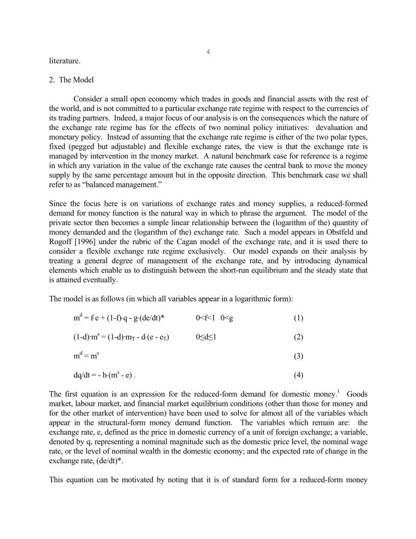
4literature. 2. The Model Consider a small open economy which trades in goods and financial assets with the rest of the world, and is not committed to a particular exchange rate regime with respect to the currencies of its trading partners. Indeed, a major focus of our analysis is on the consequences which the nature of the exchange rate regime has for the effects of two nominal policy initiatives: devaluation and monetary policy. Instead of assuming that the exchange rate regime is either of the two polar types, fixed (pegged but adjustable) and flexible exchange rates, the view is that the exchange rate is managed by intervention in the money market. A natural benchmark case for reference is a regime in which any variation in the value of the exchange rate causes the central bank to move the money supply by the same percentage amount but in the opposite direction. This benchmark case we shall refer to as “balanced management.” Since the focus here is on variations of exchange rates and money supplies, a reduced-formed demand for money function is the natural way in which to phrase the argument. The model of the private sector then becomes a simple linear relationship between the (logarithm of the) quantity of money demanded and the (logarithm of the) exchange rate. Such a model appears in Obstfeld and Rogoff [1996] under the rubric of the Cagan model of the exchange rate, and it is used there to consider a flexible exchange rate regime exclusively. Our model expands on their analysis by treating a general degree of management of the exchange rate, and by introducing dynamical elements which enable us to distinguish between the short-run equilibrium and the steady state that is attained eventually. The model is as follows (in which all variables appear in a logarithmic form): md = f⋅e + (1-f)⋅q - g⋅(de/dt)* 0<f<1 0<g (1) (1-d)·ms = (1-d)·mT - d⋅(e - eT) 0≤d≤1 (2) md = ms (3) dq/dt = - h⋅(ms - e) . (4) The first equation is an expression for the reduced-form demand for domestic money.1 Goods market, labour market, and financial market equilibrium conditions (other than those for money and for the other market of intervention) have been used to solve for almost all of the variables which appear in the structural-form money demand function. The variables which remain are: the exchange rate, e, defined as the price in domestic currency of a unit of foreign exchange; a variable, denoted by q, representing a nominal magnitude such as the domestic price level, the nominal wage rate, or the level of nominal wealth in the domestic economy; and the expected rate of change in the exchange rate, (de/dt)*. This equation can be motivated by noting that it is of standard form for a reduced-form money

5demand function. If demand for money is interest rate sensitive, then the uncovered interest rate parity condition argues that the expected rate of a depreciation of domestic currency should appear negatively as an argument, as equation (1) indicates. A similar argument from the currency substitution literature (for example, see Girton and Roper [1981]) would claim that this dependence may be a direct one, without needing the intermediation of interest-bearing financial instruments. The (logarithm of the) level of the exchange rate appears positively in the reduced-form demand for money function (as it does in the Obstfeld/Rogoff formulation). The reason is that there are a number of mechanisms, such as purchasing power parity and demand-side substitution effects as a result of changing real exchange rates, which dictate that, other things equal, a higher value for the exchange rate means a greater quantity of money is demanded. In keeping with the overshooting result (Dornbusch [1976]) which is so often cited in this literature, it is assumed that an increase in the exchange rate increases the quantity of money demanded somewhat less, so that f is taken to a positive value but less than one. That is, a given percentage increase in the level of the money supply, other things equal, causes the exchange rate to rise by a greater percentage amount. The last variable in equation (1) is the nominal magnitude q, which is given at a point in time. The coefficient on q is positive, of magnitude (1-f), reflecting monetary neutrality considerations. If both nominal magnitudes in this equation, e and q, are increased by the same amount (so that their levels are increased by the same percentage amount), then for a given degree of depreciation of the currency, the quantity of money demanded as well increases by that amount. Equation (4) shows the way in which q moves over time. Its dependence on the real quantity of money (m - e), mirrors the way in which such nominal variables as domestic prices, wage levels, or nominal wealth have been portrayed in the literature. Equation (2) captures the central bank's management of the exchange rate. Knowing that the quantity of money demanded depends positively on the exchange rate, the central bank realises that by providing a negative relationship between the quantity of money supplied and the exchange rate they will establish a unique equilibrium in the face of any shock. Furthermore, such a relationship causes the movements of the exchange rate or the money supply to be somewhat more limited than they would be under a polar exchange rate regime of either completely fixed or completely floating exchange rates. Such management is always trading off deviations of the money supply, ms, from its target value, mT, against deviations of the exchange rate, e, from its target value, eT. We assume that the private sector does not know the values of eT and mT. As a result these magnitudes do not appear in the reduced-form money demand equation or in the dynamical equation for q. Equation (2) can be written as follows: µ = µT (4a) where µ ≡ (1-d)·ms + d·e and µT ≡ (1-d)·mT + d·eT. The value of parameter d determines the extent to which exchange rates are managed. When d is

6equal to zero, there is no management of the exchange rate, although the central bank does have complete control of the money supply (so that ms = mT). When d is equal to one, the exchange rate is always kept at its target value, although the money supply can then range freely away from its target. A benchmark to which we will refer is the balanced management of the exchange rate, which is the case of d = ½. In this case, equation (2) becomes ms = mT - (e - eT). (2a) Obviously in this case the deviations of the money supply and the exchange rate from their target values are equal, but are of opposite sign. For example, an equilibrium consistent with this benchmark is one in which the level of the money supply exceeds its target value by five percent, while the exchange rate falls short of its target value by five percent. It is assumed that the economy starts off in equilibrium in which the values of the targets are equal to zero, as is the expected rate of depreciation of the domestic currency. In this situation the value of all variables is equal to zero. With this value for all magnitudes, it is natural to interpret this model as providing a description of the deviation of all variables from the values which they would have otherwise had, if the authorities had not engaged in a policy initiative at time to. Throughout this paper our focus is on the values which the exchange rate and the money supply attain in order to establish an equilibrium. Our concentration on these central variables should not cause us to lose sight of an important fact. Namely, when comparing two different situations generated by central bank actions, in our framework, if either of the two central variables, e or ms, takes on the same value in the two cases, then the other variables do likewise. Furthermore, this correspondence holds true for all the endogenous variables in the system. The reason for this phenomenon is that the exogenous variables eT and mT appear only in equation (2) and not in any of the structural form equations that describe the private sector and went into the derivation of equation (1). As a result, changes in eT and mT do not alter the isomorphism between the values of e or ms and all the other endogenous variables which are solved out in the process of deriving equation (1). That is, once we solve for the values of e or ms, we can "back out" the values of the subsidiary variables such as the interest rate, the current account balance, output, and the price level. The only requirement is that we have access to the equations of the structural form which were used to formulate equation (1). 3. A Comparison of Devaluation and Monetary Policy in the Simplest Case. The simplest model for comparing our two policy initiatives, devaluation and monetary expansion, is one which is consistent with early developments in international finance. It is the system of equations above with the assumption that (de/dt)* is exogenous, or, equivalently, that g = 0. The theory of devaluation, as represented by the contributions of Dornbusch [1973] and Mundell [1968, 1971], does not take account of possible future movements in the exchange rate. Similarly, until Dornbusch's [1976] seminal work, monetary policy was analysed with the assumption that the

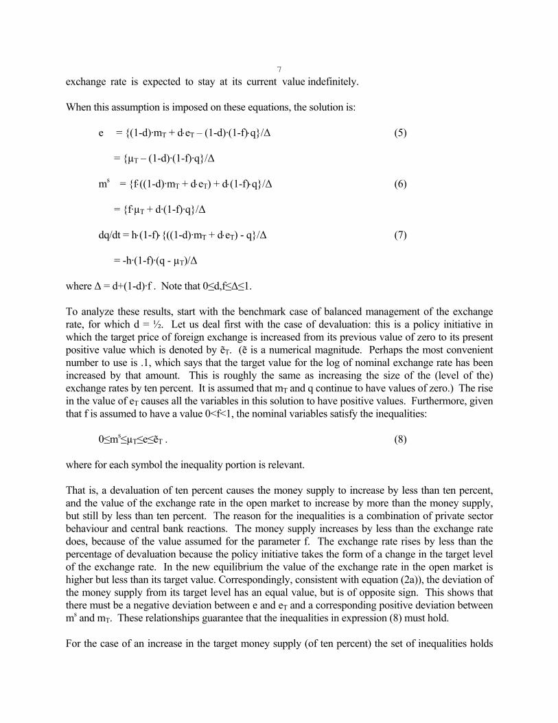
7exchange rate is expected to stay at its current value indefinitely. When this assumption is imposed on these equations, the solution is: e = {(1-d)·mT + d⋅eT – (1-d)·(1-f)⋅q}/∆ (5) = {µT – (1-d)·(1-f)·q}/∆ ms = {f⋅((1-d)·mT + d⋅eT) + d⋅(1-f)⋅q}/∆ (6) = {f·µT + d·(1-f)·q}/∆ dq/dt = h⋅(1-f)⋅{((1-d)·mT + d⋅eT) - q}/∆ (7) = -h·(1-f)·(q - µT)/∆ where ∆ = d+(1-d)·f . Note that 0≤d,f≤∆≤1. To analyze these results, start with the benchmark case of balanced management of the exchange rate, for which d = ½. Let us deal first with the case of devaluation: this is a policy initiative in which the target price of foreign exchange is increased from its previous value of zero to its present positive value which is denoted by ẽT. (ẽ is a numerical magnitude. Perhaps the most convenient number to use is .1, which says that the target value for the log of nominal exchange rate has been increased by that amount. This is roughly the same as increasing the size of the (level of the) exchange rates by ten percent. It is assumed that mT and q continue to have values of zero.) The rise in the value of eT causes all the variables in this solution to have positive values. Furthermore, given that f is assumed to have a value 0<f<1, the nominal variables satisfy the inequalities: 0≤ms≤µT≤e≤ẽT . (8) where for each symbol the inequality portion is relevant. That is, a devaluation of ten percent causes the money supply to increase by less than ten percent, and the value of the exchange rate in the open market to increase by more than the money supply, but still by less than ten percent. The reason for the inequalities is a combination of private sector behaviour and central bank reactions. The money supply increases by less than the exchange rate does, because of the value assumed for the parameter f. The exchange rate rises by less than the percentage of devaluation because the policy initiative takes the form of a change in the target level of the exchange rate. In the new equilibrium the value of the exchange rate in the open market is higher but less than its target value. Correspondingly, consistent with equation (2a)), the deviation of the money supply from its target level has an equal value, but is of opposite sign. This shows that there must be a negative deviation between e and eT and a corresponding positive deviation between ms and mT. These relationships guarantee that the inequalities in expression (8) must hold. For the case of an increase in the target money supply (of ten percent) the set of inequalities holds

8(8), with m̃T substituting for ẽT: 0<ms<µT<e<m̃T . (9) Indeed, when d = ½, there is no difference in value for any of the coefficients on m̃T and those on ẽT. A ten percent increase in the money supply has precisely the same observable effects as does a ten percent devaluation. There is a difference between the two in terms of the unobservable variables. Most obviously, with monetary policy mT increases while eT remains at zero, whereas with devaluation eT increases while mT remains the same. Accordingly, for devaluation there is a negative deviation between e and eT, and a concomitant positive deviation between m and mT. In contrast, for expansionary monetary policy there is a negative deviation between m and mT, and a corresponding positive deviation between e and eT. The reader can establish that the inequalities of (8) continue to hold for all values of d such that 0≤d≤1. In contrast, the inequalities of (9) are correct when d>(1-f)/(2-f). For smaller values of d, the relationships are instead: 0≤ms≤µT≤m̃T≤e (10) The conclusion can be stated quite succinctly. When expectations of future exchange rate movements can be ignored, for the case of balanced management of the exchange rate (for which d = ½), monetary policy and devaluation of equal percentage amounts have identical impacts on observable variables. An increase in the target money supply by the amount ẽT (for example, ten percent) generates identical results to a (ten percent) devaluation of amount ẽT. As noted above, if the money supply or the exchange rate takes on the same value in response to these two initiatives, then all other endogenous variables do too. The equilibria are the same in terms of observable variables. They differ only insofar as the values of mT and eT, both of which are not observable, have different values in the two cases. Inspection of equations (5)-(7), demonstrates the more general result that in the case where monetary policy and devaluation are carried out in a setting in which the degree of management of the exchange rate is given at a value of d, then a monetary policy initiative which increases the target money supply by the amount (d/(1-d))⋅ẽT has identical effects as a devaluation of amount ẽT. This result is consistent with our intuition: when a high degree of management of the exchange rate is being carried out (so d≈1, and the regime is very close to fixed exchange rates), then only a massive increase in the target money supply will generate equivalent results. In this case when the policy initiative is in the form of a ten percent devaluation, the increase in the market value for the exchange rate is very close to the increase in the value for the target exchange rate (so that the deviation between the two is quite small). In contrast there is an appreciable deviation between money supplies (although somewhat less than ten percent), reflecting the increase in the actual money supply with no change in its target level. Also, in this case (d≈1) when identical results are obtained via a monetary policy initiative, the target

9value of the money supply must be increased a lot more than ten percent. From this initiative there results a massive negative difference between the value of the actual money supply (which (being an observable magnitude) increases precisely as much as it does when devaluation is the initiating policy) and its target level, and this translates into an exchange rate deviation of somewhat less than ten percent. The reason is that now the actual value of the exchange rate increases as much as it does with devaluation (again, it is an observable variable), while the target value of the exchange rate has not changed with this policy initiative. 4. Monetary Policy and Devaluation under Differing Degrees of Management of the Float The discussion in the previous section showed that, so long as the expected rate of change of the exchange rate can be safely ignored, for any finite degree of management of the exchange rate, there is a monetary policy initiative which has identical observable effects as a given percentage devaluation. The question here is whether, if we continue with the assumption about expectations of future exchange rate changes, we can generalise these results so that comparisons of these two initiatives can be made when there are differing degrees of management of the exchange rate. In its starkest terms, the question can be phrased in terms of the polar exchange rate regimes as follows: Is monetary policy under flexible exchange rates observationally equivalent to devaluation under fixed exchange rates? We will find that the answer to this question is in the affirmative. This experiment sets out, once again, the temptation which Allen and Kenen presented a quarter century ago.2 Is it true that an open market operation under flexible exchange rates has the same effect as a devalution under fixed exchange rates? To this question, we unambiguously answer yes, so long as the market in which the exchange rate is being stabilized is the same as the market in which the open market operation is conducted. The reason that Allen and Kenen argue that we should not yield to this temptation is that there are “…differences…[between these two actions that]…are not negligible….the analogy is imperfect…[it]…has been overdrawn…” according to the results of their model, except when there is perfect capital mobility (or when domestic bonds are effectively denominated in foreign currency). In turn, the explanation for these differences is that the open market operation is viewed as being carried out in the money-capital market (a purchase of domestic government bonds in exchange for money) whereas pegging of the exchange rate is carried out in the foreign exchange market (so that foreign exchange instruments are bought and sold in exchange for money). When there is perfect capital mobility, foreign exchange and domestic bonds are perfect substitutes so that effectively these two operations are identical.3 We deal with the Allen-Kenen question in the situation in which the degree of stabilization of the exchange rate is quite general in each case, and in which the degree can differ between the economy in which the devaluation is occurring as compared with that in which money policy is being carried out. In order to answer this question for the general case, we return to the structural equations (1) - (4), and assume that the policy initiatives are conducted independently. That is, they are conducted in otherwise identical economies (so the values of the parameters f and h are the same), but in the case of a monetary policy initiative, the value of the managed floating parameter is equal to dm; whereas in the case of a devaluation, the value of the managed floating parameter is equal to de.

10 Solving for the effects on the observable variables for the two initiatives independently we find: In the case of a monetary initiative e = (1-dm)·m̃T/∆m (11) m = f⋅(1-dm)·m̃T/∆m (12) dq/dt = h⋅(1-f)⋅(1-dm)·m̃T/∆m (13) where ∆m = (dm+(1-dm)·f). In the case of a devaluation e = de⋅ẽT/∆e (14) m = f⋅de⋅ẽT/∆e (15) dq/dt = h⋅(1-f)⋅de⋅ẽT/∆e (16) where ∆e = (de+(1-de)·f). Clearly every variable in the case a devaluation has the same value which it did with a monetary initiative multiplied by the factor ((de/(1-dm))⋅∆m/∆e. It follows that, when the degree of management of the exchange rate is dm, a monetary policy initiative of amount ((de/(1-dm))⋅∆m⋅ẽT/∆e, has precisely the same effects as a devaluation of amount ẽT does when the degree of management of the exchange rate is equal to de. Let us focus on the polar exchange rate cases, for the situations where the results are not degenerate. Starting with monetary policy under flexible exchange rate, we are considering a situation in which dm is equal to zero, so that ∆m is equal to f. We want to compare that with devaluation under fixed exchange rates, so that de = 1. For this case, ∆e too has a value of 1, so the ratio of de/∆e has a value of one. The conclusion of this analysis is that a monetary policy initiative under flexible exchange rates of something less than ten percent (specifically the amount f times ten percent) will have results which are observationally identical to those which a ten percent devaluation under a fixed exchange rate regime would generate. These are demonstrations of the robust conclusion that so long as expectations of future movements of the exchange rate can be ignored, monetary policy and devaluation are identical policy initiatives even if they are enacted under conditions which differ considerably as to the degree of management of the float. In all cases we can find an increase in the (target) money supply that has identical effects to those generated by a given percentage increase in the (target) value of the exchange rate. 5. The Berglas-Dornbusch-Mundell Result

11 We have shown above that in an economy in which the degree of management of the exchange rate is given by d a monetary policy initiative of amount ẽT has the same effect on all variables, including real ones, as a devaluation of the amount ((1-d)/d)·ẽT. Thus when d=½, a ten percent increase in the target money supply (an expansionary monetary policy) has observationally equivalent effects as a ten percent increase in the target value for the exchange rate (an equiproportionate devaluation). This is true for both nominal variables and real ones. This conclusion seems to be at variance with the conclusion of Berglas [1974], Dornbusch [1973] and Mundell [1967, 1971] that a ten percent devalution has the same effect on real variables as a ten percent decrease in the money supply. The intuition is that a devaluation depresses the quantity of real money through a price shock, and equivalent results will occur through a quantity of money shock so long as it has the same impact on the real quantity of money.4 That there is no conflict between their results and ours can be verified by writing down a real variable, which here is the deflation of the nominal money supply by the exchange rate. The expression for this magnitude, as in equation (7), is: m – e = (f-1)(µT – q)/∆ (17) This real variable is to be viewed as a synedoche for real variables in general. We see from this expression that its value depends upon the difference between the value of µT and the value of q, which here is most conveniently thought of as being nominal wealth. This expression shows that an increase in µT of a given (percentage) amount has the same effects on all real variables as a decrease in q of that (same percentage) amount. This is the result which Berglas-Dornbusch-Mundell have derived, but they are dealing with a special case of our model. They have assumed that the exchange rate is rigidly pegged at a point in time, although the value of the exchange rate peg can be altered, as, of course, a devaluation exemplifies. In terms of our notation, they are assuming that d = 1. But they are further assuming that there is only one nominal asset in the system, money, so that the only way in which ms can change is for q to change by an equal amount. The explanation for this Berglas-Dornbusch-Mundell result is simple. The reason that devaluation and an equal percentage change of opposite sign in the money supply have the same effects on all real variables is that in their model one is comparing devaluation with an equal percentage change (of opposite sign) in wealth. This conclusion falls immediately out of a model that is homogeneous of degree one in all nominal variables. Effectively their model has only two short-run exogenous nominal variables: e and q. In contrast, our model has three such variables: eT, m T, and q. We have shown observational equivalence between a change in the target exchange rate of ẽT and a change in the target money supply of the amount d·ẽT/(1-d) (that is, changes which have the same impact on µT). We have also shown equivalence in terms of effects on real variables of changes in µT and those (of opposite sign) of q. But changes in q, for us, are not monetary changes. Money is an endogenous variables in an open economy (as Dornbusch and Mundell have emphasised in so many different contexts, but not in their analyses of devaluation). In contrast, wealth is validly treated as

12an exogenous variable in the short run in an open economy. 6. The Path of Adjustment The model includes a nominal magnitude, q, which has a given value in the short run. However, in the long run, q adjusts to its steady-state value, from which it will not move until the economy is impacted by a further shock. To find the speed of adjustment of the economy from a short-run equilibrium to the steady state we need to take the time derivative of the model with which we have been working. We assume that also during the path of adjustment the authorities manage the exchange rate by intervening in the money market. As a result equation (3) continues to hold, although we permit the possibility that the exchange rate management parameter has a different value during the adjustment process: to take account of this possibility the value of the parameter is denoted by d' during this period. Equating the supply of money (equation (2)) to the demand for money (equation (1)) and time differentiating the resulting equation, we find (1-d’)·g⋅(d2e/dt2) - (d'+(1-d’)·f)⋅(de/dt) - (1-f)⋅h⋅e = 0 (18) (where e is now measured relative to its steady-state value). This equation assumes that expectations are rational, more specifically that there is perfect foresight. It is for this reason that the actual rate of change of the exchange is substituted for the expected rate of change. In taking account of changing expectations, we have moved beyond the discussion in the previous sections of this paper. The solution to such a second order differential equation is of the form: e = A⋅exp(δ1⋅t) + B⋅exp(δ2⋅t) (19) and the values of the δ's are the solutions of the quadratic equation (1-d’)·g⋅δ2 -(d'+(1-d’)·f)⋅δ - (1-f)⋅h = 0 . (20) In turn the solutions to the quadratic equation are equal to: δ1,2 = {(d'+(1-d’)·f) ± [(d'+(1-d’)·f)2 + 4⋅g⋅(1-f)⋅h]½/((2⋅g)·(1-d’)) (21) We will assume that there are no speculative bubbles, so the solution we focus on has the following value for δ: δ = {(d'+(1-d’)·f) - [(d'+(1-d’)·f)2 + 4⋅g⋅(1-f)⋅h]½/((2⋅g)·(1-d’)) (22) Furthermore, for small values of g and h, this simplifies to δ = - (1-f)⋅h/(d'+(1-d’)·f). (23)

13This shows that the speed of adjustment is independent of the value of g for small values of this parameter. It should be noted that if the degree of management of the float during the adjustment process differs from that during the initial response to a shock, it is the degree of management during the adjustment process which is the determinant of the speed of adjustment. This observation is important to understanding some results which are derived below. Finally, the speed of adjustment depends upon the degree of management of the float. With the parameter f having a positive value less than one, it is straight forward that the higher the value of d', the smaller is the (absolute) value of δ. This shows that flexible exchange rate systems have more rapid convergence than do fixed exchange rate ones. This conclusion points out that observational equivalence will no longer hold over the path of adjustment if different degrees of management of the exchange rate are employed. This conclusion does not make any statement about the nature of the policy initiatives, which could be identical. It is a statement about the consequences of any action when differing exchange rate regimes are followed during the process of adjustment. For example monetary policy has effects during the process of adjustment when there is balanced management, which are different from its effects when the exchange rate is allowed to float freely. 7. The General Solution When Differing Degrees of Management are Employed So far our comparative static results have been confined to the case in which expectations of future movements of the exchange rate are taken given, or equivalently when expected movements have no effects on financial markets. This is the case represented by g = 0. These assumptions provided a fruitful starting point because they enabled us to make comparisons with conclusions in the literature of international finance. But these assumptions are hardly realistic in the present world in which capital flows and portfolio balance considerations seem to be the most important elements in explaining exchange rate movements. With the introduction of expectations into the analysis, our central question returns: under what circumstances are devaluation and monetary policy observationally equivalent? The discussion in the previous section hints at the correct answer: when the degree of management of the exchange rate during the adjustment process is identical for these two initiatives, then they maintain their observational equivalence. To confirm this conclusion we need to derive the general result in which the degree of management of the exchange rate takes on four possible values: one for each of the initiatives, and, in each such case, for the two time periods; for the initial jump to a new short-run equilibrium, and for the process of adjustment. In all cases we are focussing on the value of d. As before subscripts denote the value which d has depending upon whether a devaluation initiative is undertaken (de) or a monetary policy initiative is undertaken (dm). Unprimed d parameters refer to values which hold during the instantaneous jump, and primed d parameters refer to values which hold during the adjustment process. (For example, de‘ refers to the degree of management of the float during the adjustment process when a devaluation initiative is undertaken.)

14 The key to solving the model for this case is to note that in the short run after the instantaneous jump, the economy satisfies three conditions. First, the private sector, consistent with its constraints (namely that q is a given during this timeframe and that expectations must be consistent with what actually transpires), must be maximising its objective function. Specifically, this implies that equation (1) is satisfied. In addition, the short-run equilibrium must be consistent with the central bank's instantaneous reaction function. The reaction function is designed to cope with and counter sudden changes in the value of the exchange rate, of which the present shock (even though originating in the government sector) is a clear example. Finally, the short-run equilibrium must be on the reaction function to which the authorities will adhere during the adjustment process. (Perhaps a further condition worth mentioning is that in the new steady state, which must also be consistent with the adjustment-process reaction function, all nominal variables, e, m and q have increased by the same (percentage) amount.) Specifically the equations which are satisfied are -d/(1-d)⋅(e0 - eT) = f⋅e0 + [g⋅(1-f)⋅h)⋅(e0-eT)]/(f·(1-d’)+d') mT + (d/(1-d))·(eT-e0) = f·e0 + g·δ·(e0-eλ) (24) The left-hand-side of this equation is the money supply using instantaneous jump reaction function, where we have denoted the short-run value of the exchange rate by e0. The right-hand-side is the demand for money in the short run (for which q = 0), and in which the expected rate of change of the exchange rate (de/dt) has been written in the form δ⋅(e0 - eλ), where eλ is the long-run value which all nominal variables attain. The second equation is: (1-d)·mT + d·eT = (1-d)·m0 + d·e0 (25) This equality is a repeat with current notation of equation (4a). Finally, we have (1-d’)·m0 + d’·e0 = eλ . (26) This equation states that the value of the monetary target index using the weights along the path of adjustment equal the value of the index at the long-run equilibrium. In that equilibrium the value of all nominal variables is eλ, so likewise is the value of the index. The solution to these equations in the short run is e0 = µT·(1+(1-d’)·g·δ)/∆λ (27) m0 = µT·(f +(1-d’)·g·δ)/∆λ (28)

15 where ∆λ = d + (1-d)·f + (1-d’)·g·δ. These solutions demonstrate that so long as the same degrees of management of the exchange rate (for the instantaneous jump and during the process of adjustment) are in force, a monetary policy initiative is observationally equivalent to a devaluation. It should be noted that this result does not depend on the degree of jump management being equal in value to the degree of intertemporal management. 8. Management during the Path of Adjustment As before let us deal with our two initiatives separately, assuming that the degree of management is dependent upon the initiative undertaken. In that case we find the following expressions for e0 and m0. For the case of devaluation: e0 = de⋅eT·(1+g·δe·(1-de’))/∆e (29) m0 = de⋅eT·(f+g·δe·(1-de’))/∆e (30) where ∆e = d+(1-d)·f+g·δe·(1-de’) For the case of monetary policy: e0 = (1-dm)·mT·(1+g·δm·(1-dm’))/∆m (31) m0 = e0 = (1-dm)·mT·(f+g·δm·(1-dm’))/∆m (32) where ∆m = d+(1-d)·f+g·δm·(1-dm’) It is straight forward to note that when the degree of management of the exchange rate is same along the adjustment path, so that de' = dm' (≡ d'), there continues to be observational equivalence. That is a value of m̃T equal to de·ẽT·∆m/((1-dm)·∆m generates the same values for e0 and m0 (and for all other magnitudes in the economy) as does a devaluation of amount ẽT. This shows that observational equivalence does not hinge upon there being the same degree of management during the instantaneous jump. But obviously this observation raises the question as whether equivalence continues to hold when there are different degrees of management during the path of adjustment. The easiest way to show this to calculate the ratio e0/m0 for the two policy initiatives.

16 For monetary policy this ratio is equal to {e0/m0}m = (1+g·δm·(1-dm’))/(f+g·δm·(1-dm’)) (33) whereas for devaluation this ratio is equal to {e0/m0}e = (1+g·δe·(1-de’))/(f+g·δe·(1-de’)) (34) These expressions show that these ratios satisfy the following inequalities: 1<{e0/m0}m<{e0/m0}e<1/f if dm'<de'. The middle inequality sign needs to be reversed if de'<dm'. And it needs to be changed to an equality sign if de'=dm’. This analysis shows that a necessary condition for observational equivalence is equality of the degree of intertemporal management of the exchange rate. In contrast, the degree of instantaneous management of the exchange rate is irrelevant for observational equivalence. The instantaneous degree is a determinant of the size of the initiative which needs to be undertaken in order to generate identical results. But since the size of the initiative is not known to the public, this does not violate observational equivalence. In contrast the degree of intertemporal management determines not only the size of the instantaneous movements of the exchange rate and the money supply but also the proportions in which they move. As a result observational equivalence no longer holds when the degree of management is dependent on the policy initiative which is undertaken. 9. Literature Review Beginning with the Mundell-Fleming model, the literature in international finance has analyzed policy actions under the polar regimes of fixed and flexible exchange rates. For example, it is a commonplace in standard textbooks to contrast the efficacy of monetary policy under a flexible exchange rate regime with its impotence under a fixed rate regime. This paper argues that in order to probe the symmetry of policy actions and the circumstances when those actions yield equivalent results, it is appropriate to employ a regime of managed floating, since in this case the policies under study typically have non-degenerate effects. In particular expansionary monetary policy under a managed floating regime will have an impact on the economy so long as the degree of management is bounded. Our specific interest is in the circumstances under which devaluation and monetary policy have observationally equivalent effects. The conclusion is that under simple conditions, there is a percentage increase in the money supply which has identical effects on all observable variables as a given percentage of devaluation. This conclusion points out that although these initiatives are

17identified by different names, in fact they are exactly the same policy. The intuition behind this result is quite simple: as with any monopolist, a Central Bank's decision to alter the price of its product, is simultaneously a decision to alter the quantity of production, and vice versa. In open economy monetary economics, the close connection between decisions about price (the exchange rate) and those about quantity (the size of the money supply) have been remarked on for at least one hundred years. Thus, Keynes [1924] talking about the foreign exchange value of the French franc refers to the "first principles" derived from his Tract on Monetary Reform as indicating a simple relationship between the exchange rate and the quantity of money.5 Sufficient conditions for observational equivalence to hold are: that the markets of intervention to manage the exchange rate be the same as the markets in which policy initiatives are undertaken; and that the same finite degree of management of the exchange rate be used for the two policies. While the first condition seems essential for this equivalence, the second is not necessary. So long as one deals with a specific timeframe, equivalence continues to hold independent of the exchange rate regime. However, once one considers alternative timeframes and the process of adjustment in moving between them, then clearly differences do arise. But these differences are not due to the policies per se but are instead due to the fact that the nature of the economy's adjustment path depends upon the exchange rate regime which is in force. This simple equivalence result contrasts with the separate paths which analyses of these two policy initiatives have followed in recent times. The most dramatic statement of the contrary point of view was made by Johnson [1958]. In it, he contends that these two policies fall into disjoint categories: devaluation is an "expenditure-switching" device; whereas "monetary restriction" is an "expenditure-changing" one. This categorisation has had a major impact on discussion of these issues right up to the present, as is exemplified by Frankel [2004]. Specifically textbooks continue to follow this line of thinking perpetuating the claim that monetary actions and devaluation are different policy instruments. Thus, Kenen [1994, pp 362-6], Ethier [1995, pp 519-20], Caves, Frankel and Jones [1996, pp 407-9], and McCallum [1996, pp 143-4] claim that devaluation can be undertaken without short-run monetary effects. For example, Kenen develops a diagram (page 363) in which expenditure policy is on the vertical axis and the exchange rate is on the horizontal axis. The two variables can be changed independently in an economy because "Its government pegs the exchange rate but is free to change the peg...Its central bank controls the money supply..." Ethier finds that devaluation causes a balance of payments surplus that will increase the money supply over time unless sterilised. In contrast, monetary policy sets up a temporary equilibrium which prevails only until domestic citizens have bought enough bonds from abroad to replace those sold to the authorities p 56. Finally, Caves, Frankel and Jones p408 and McCallum pp 143-4 envisage a devaluation without any shift in the LM curve. Of greater consequence, all these authors claim that devaluation and monetary policy have the opposite effects on various accounts of the balance of payments. Dealing with the current account, Caves, Frankel and Jones [pp 405, 424 and (in a different framework) p 443] finds that a monetary expansion causes a deficit, while devaluation causes a surplus [pp 408, 427 and 444]. Kenen makes the same claim on pp 363-369, as does Ethier on p 519. McCallum does not deal with

18the Current Account, but does find that expansionary monetary policy leads to an official settlements deficit, whereas a devaluation draws in reserves from abroad. In so far as these textbooks are representative of thinking about policies in the open economy, it is fair to say that the standard view at the present time is that devaluation and expansionary monetary policy are two independent policies with very different consequences. Therefore, the conclusions of this paper are directly at variance with the prevailing view.6 10. Conclusion This paper has found that devaluation and expansionary monetary policy have very similar effects in standard models of a small open economy which stabilises its exchange rate to a degree that is set parametrically. When expectations are myopic the key condition that must be met is that the markets for intervention to stabilise the exchange rate must be the same as those in which the monetary initiative is carried out. An alternative assumption, made by a number of well-known economists, is that there exists only one financial instrument in the economy and that pegging of the exchange rate takes places in the goods market. Such models arrive at conclusions which are diametrically opposed to what we find here and to what is observed in the data. In a model with perfect foresight, a subsidiary condition for observational equivalence is that the degree of management of the float during the process of adjustment to long run equilibrium be the same for these two policy initiatives. The identity we find between expansionary monetary policy and devaluation presents a dilemma when one looks at recent research in the theory of devaluation. This research (Frankel [2004]) continues to find that devaluation can be contractionary (as Cooper [1971] reported more than thirty years ago. Yet no economist believes expansionary monetary policy to be contractionary. Obviously there is a contradiction here: one with which we intend to deal in our next paper on this subject.

19References Allen, Polly and Kenen, Peter [1980], Asset Markets, Exchange Rates, and Economic Integration: A Synthesis, Cambridge University Press. Berglas, Eitan [1974], “Devaluation, monetary policy, and border tax adjustments,” The Canadian Journal of Ecomics, VII, 1(February), 1-11. Caves, Richard, Frankel, Jeffrey, and Jones, Ronald [1996], World Trade and Payments: An Introduction, seventh edition, Harper Collins. Cooper, Richard [1971], “Currency devaluation in developing countries,” Essays in International Finance, 86, Internal Finance Section, Princeton, N.J. Dornbusch, Rudiger [1973], "Currency depreciation, hoarding and relative prices, Journal of Political Economy, 81, 5(October), 893-915. ----------- [1976], "Expectations and exchange rate dynamics," Journal of Political Economy, 84, 6(December), 1161-76. Ethier, Wilfrid [1995], Modern International Economics, third edition, W W Norton. Fleming, J Marcus [1962], "Domestic financial policies under fixed and under floating exchange rates," International Monetary Fund Staff Papers, 9 (November), 369-79. Frankel, Jeffery [2004], “Contractionary currency crashes in developing countries,” The 5th Mundell-Fleming Lecture, IMF Annual Research Conference, IMF Staff Papers, forthcoming. Frenkel, Jacob and Johnson, Harry, eds [1977], The Monetary Approach to the Balance of Payments, University of Toronto Press. Frenkel, Jacob, and Mussa, Michael [1985], “Asset markets, exchange rates, and the balance of payments,” in Jones, Ronald W. and Kenen, Peter B. (eds.) Handbook of International Economics, volume 2, North-Holland, Amsterdam, chapter 14 (679-747). Girton, Lance and Roper, Don [1981], "Theory and implications of currency substitution," Journal of Money, Credit and Banking, 13, 1(February), 12-30. Harberger, Arnold C. [1950], Currency depreciation, income and the balance of trade," Journal of Political Economy, 58, 1(February), 47-60. Helpman, Elhanan [1981], "An exploration of the theory of exchange rate regimes," Journal of Political Economy, 89, 5(October), 865-90. Johnson, Harry [1958], "Toward a general theory of the balance of payments," Trade and Economic

20Growth. Reprinted in Jacob Frenkel and Harry Johnson, eds, [1977], The Monetary Approach to the Balance of Payments, University of Toronto Press. Kenen, Peter B. [1994], The International Economy, third edition, Cambridge University Press. Keynes, John Maynard [1924], "Commentary" from The Nation and Athenaeum, March 15, 1924. As reprinted in The Collected Works of John Maynard Keynes, [198?], Macmillan and The Cambridge University Press for the Royal Economic Society, Volume XIX, part 1, p 177. Lucas, Robert [1976], "Econometric policy evaluation: a critique." In Karl Brunner and Allan H. Meltzer, eds., The Phillips Curve and Labour Markets. Amsterdam: North Holland. McCallum, Bennett [1996], International Monetary Economics, Cambridge University. Mundell, Robert A. [1963], "Capital Mobility and Stabilization Policy under Fixed and Flexible Exchange Rates," Canadian Journal of Economics and Political Science, 29 (November), 475-85. ______________, [1967] "International Disequilibrium and the Adjustment Process," in John H Adler (ed), Capital Movements and Economic Development, St Martin's Press, New York, pp 441-62. Printed in an adapted form as "Barter theory and the monetary mechanism of adjustment," in Mundell, Robert A. [1968], International Economics, Macmillan, Chapter 8. ------------ [1971], Monetary Theory, Goodyear Publishing, Pacific Palisades, CA. Obstfeld, Maurice and Rogoff, Kenneth [1996], Foundations of International Macroeconomics, MIT Press, Cambridge, MA. Salvatore, Dominick [1998], International Economics, 6th edition, Prentice Hall, Upper Saddle River, N.J. Tsiang, S. C. [1961], “The role of money in trade-balance stability: synthesis of the elasticity and absorption approaches,” American Economic Review, 51, 912-36, Footnotes 1 The model implicitly assumes that the markets of intervention to stabilize the exchange rate are the same as the markets in which the monetary policy initiative is carried out. It this is not true, then the excess demands created in differing markets will cause the demand function for money (equation (1)) to shift in one case and not in the other. The equivalence between devaluation and monetary policy would thereby be negated. 2 Allen and Kenen [1980, 40] assume that the exchange rate is pegged by intervention in the foreign exchange market, while an open market operation is conducted in the domestic bond market. In contrast, we are assuming in this paper that the pegging operation is carried out in the same market as the open market operation. This is a key assumption guaranteeing the

21 equivalence of the two policy initiatives which we consider. In the limit of perfect capital mobility, these two markets are effectively the same, and Allen and Kenen come to the same conclusion as do we. 3 This conclusion side-steps some of the issues which Allen and Kenen raise concerning monetary neutrality in an economy in which there exist two domestic-currency-denominated market instruments. It is precisely these issues which causes these authors to conclude that the differences between devaluation and monetary policy as not being negligible, since monetary neutrality holds in one case but not the other. The reconciliation with the analysis in the present paper is that when the open market operation is carried out in the foreign exchange market (which Mundell [1963] calls “an alternative form of monetary policy”), then the effects are precisely the same as a devaluation (since all modelers are picturing the exchange rate as being stabilized by interventions in the foreign exchange market). 4Mundell [1967, 1971] does not specify how the exchange rate is pegged in his analyses. Dornbusch [1973] states specifically that domestic money is bought and sold for foreign exchange. But since foreign exchange is not held by domestic residents (nor is domestic money held by foreign residents), by pegging the exchange rate the authorities are setting the domestic-currency price of foreign goods. Therefore they are effectively intervening in the foreign goods-domestic money market. The results that Berglas-Dornbusch-Mundell report are thus relevant for economies that peg the exchange rate by intervention in the money-goods market. 5.. 5..Keynes [1924, p 177] refers to such a relationship as being based on the "first principles" of exchange rate determination. Alluding specifically to the French franc at the time, he states that "The value of the franc will be determined, first, by the quantity, present and prospective, of the francs in circulation; and, second, by the amount of purchasing power which it suits the public to hold in that shape." 6.. The reader may note a certain similarity with the conclusions at which Helpman [1981] arrived. Our point is quite different from his in that for the two nominal shocks considered by us, the equilibria are precisely the same, rather than being so just in real terms. Only these nominal shocks generate identical results, contrary to Helpman for whom shocks of any sort have precisely the same real equilibria. Finally, Helpman's results are specific to the foreign-currency indexed economy of his model, whereas ours apply to any model which satisfy the two conditions identified above.