On the mean pro les of radio pulsars I: Theory of the ...

Mon. Not. R. Astron. Soc. 000, 000–000 (0000) Printed 30 August 2018 (MN LATEX style file v2.2)

On the mean profiles of radio pulsars I: Theory of thepropagation effects

V. S. Beskin1,2? and A. A. Philippov21P.N.Lebedev Physical Institute, Leninsky prosp., 53, Moscow, 119991, Russia2Moscow Institute of Physics and Technology, Dolgoprudny, Institutsky per., 9, Moscow region, 141700, Russia

30 August 2018

ABSTRACT

We study the influence of the propagation effects on the mean profiles of radiopulsars using the method of the wave propagation in the inhomogeneous media de-scribing by Kravtsov & Orlov (1990). This approach allows us firstly to include intoconsideration the transition from geometrical optics to vacuum propagation, the cy-clotron absorption, and the wave refraction simultaneously. In addition, non-dipolemagnetic field configuration, drift motion of plasma particles, and their realistic en-ergy distribution are taken into account. It is confirmed that for ordinary pulsars(period P ∼ 1 s, surface magnetic field B0 ∼ 1012 G) and typical plasma generationnear magnetic poles (the multiplicity parameter λ = ne/nGJ ∼ 103) the polarizationis formed inside the light cylinder at the distance resc ∼ 1000R from the neutronstar, the circular polarization being 5–20% which is just observed. The one-to-onecorrespondence between the signs of circular polarization and position angle (p.a.)derivative along the profile for both ordinary and extraordinary waves is predicted.Using numerical integration we now can model the mean profiles of radio pulsars. Itis shown that the standard S-shape form of the p.a. swing can be realized for smallenough multiplicity λ and large enough bulk Lorentz factor γ only. It is also shownthat the value of p.a. maximum derivative, that is often used for determination theangle between magnetic dipole and rotation axis, depends on the plasma parametersand could differ from the rotation vector model (RVM) prediction.

Key words: Neutron stars— radio pulsars — polarization

1 INTRODUCTION

More than forty years after discovery, our understand-ing of pulsar phenomenon leaves an ambiguous impression.On the one hand, the key properties were understood al-most immediately (see, e.g., the monographs by Manchester& Taylor 1977; Lyne & Graham-Smith 1998): the stable pat-tern of radio emission is related to the neutron star rotation,the energy source is the kinetic energy of its rotation, andthe release mechanism has the electromagnetic nature. Themean profiles of radio pulsars are well described by the hol-low cone model (see below). Within four last decades enor-mous amount of observational data concerning polarizationand other morphological properties of mean profiles was col-lected (Rankin 1983, 1990; Johnston et al. 2007; Weltevrede& Johnston 2008; Hankins & Rankin 2010; Keith et al. 2010;Yan et al. 2011). However, there is no agreement on the

? E-mail: [email protected]

mechanism of coherent radio emission (Beskin 1999; Usov2006; Lyubarsky 2008).

Any self-consistent theory of pulsar radio emission mustinclude at least three main elements. First, it should describea plasma instability that produces coherent radio emission.Second, the saturation of this instability that determines theintensity of the outgoing radio emission. Third, once the ra-diation is produced, its polarization properties are modifiedby the interaction with magnetospheric plasma and fields.These propagation effects should be accounted for to makea quantitative comparison of the theoretical predictions forthe generation of radio emission with observational data.

There are several proposed mechanisms for the initialinstability: an unstable flow of relativistic electron-positronplasma flowing along curved magnetic field lines (Goldre-ich & Keeley 1971; Blandford 1975; Asseo et al. 1980; Be-skin, Gurevich & Istomin 1993, hereafter BGI); an instabil-ity caused by boundedness of the region of open field lines(Luo, Melrose & Machabeli 1994; Asseo 1995); an instabil-ity connected with kinetic effects, that can be caused by

c© 0000 RAS

arX

iv:1

107.

3775

v2 [

astr

o-ph

.HE

] 2

4 M

ar 2

012

2 V. S. Beskin and A. A. Philippov

non-equilibrium of the particles energy distribution function(mainly, anomalous Doppler effect in the region of cyclotronresonance); two-stream instability (Kazbegi, Machabeli &Melikidze 1991); the instability connected with the nonsta-tionarity of plasma particle production in the region of itsgeneration (Lyubarskii 1996).

The saturation mechanism, whose investigation requiresinvolving the effects of a nonlinear wave interaction, is themost complex from the theoretical point of view. There-fore, it is not surprising that only a few researchers havemanaged to consider this question consistently (see, e.g., Is-tomin 1988). Finally, the processes of the wave propagationin pulsar magnetosphere have not yet been investigated withsufficient detail either, although the part of theory that in-cludes the propagation processes can be constructed usingthe standard linear methods of plasma physics.

Recall that the present interpretation of the mean pro-files of radio pulsars is based on the ground of so-calledhollow cone model (see, e.g., Manchester & Taylor 1977).Within this approach the directivity pattern is assumed torepeat the profile of the number density of secondary parti-cles outflowing along the open field lines. As the secondaryplasma cannot be generated near the magnetic pole (wherethe curvature photons radiating by primary beam propagatealmost along magnetic field lines), the particle number den-sity is to have the ’hole’ in its space distribution (Sturrock1971; Ruderman & Sutherland 1975).

There are four assumptions in the hollow cone model:first, the emission is generated in the inner magnetosphericregions (where the magnetic field may be considered as adipole); second, the emission propagates along the straightline; third, the cyclotron absorption may be neglected; andfourth, the polarization is determined at the emission point.Such basic characteristics of the received radio emission al-low to determine the change of the position angle (p.a.) ofthe linear polarization along the mean profile (Radhakrish-nan & Cocke 1969)

p.a. = arctan

(sinα sinφ

sinαcosζcosφ− sin ζcosα

). (1)

Here α is the inclination angle of the magnetic dipole to therotation axis, ζ is the angle between the rotation axis andthe observer’s direction, and φ is the pulse phase.

As a result, the radiation beam width Wr itself andits statistical dependence on the period P can be quali-tatively explained under these assumptions (Rankin 1983,1990). As the pulsar radio emission is highly polarized (Lyne& Graham-Smith 1998), one could check the validity of therelation (1) as well. As is well-known, in many cases theobserved p.a. swing is in good agreement with this theoret-ical prediction. Besides, the polarization observations showthat the pulsar radio emission consists of two orthogonalmodes, i.e., of two components which p.a. differ by 90

(Taylor & Stinebring 1986). It is logically to connect twosuch components with two normal modes, ordinary and ex-traordinary ones, propagating in a magnetoactive plasma(Ginzburg 1961). It is not surprising that the hollow conemodel in its simplest realization is currently widely usedfor quantitative determination of the parameters of neutronstars.

At the same time, it is well known that, in general,three main assumptions are incorrect. First of all, after the

paper by Barnard & Arons (1986), it became clear that theordinary wave (i.e., the wave which electric field belongs tothe plane containing the wave vector k and the externalmagnetic field B) does not propagate in a straight line, butdeflects away from the magnetic axis. Subsequently, this ef-fect was studied in detail by Petrova & Lyubarskii (1998,2000), it was an important element in the BGI theory. Thecorrection to relation (1) connected with the aberration wasdetermined by Blaskiewicz et al. (1991), but it was rarelyused in analysis of the observational data as well.

Further, the cyclotron absorption that must take placenear the light cylinder (Mikhailovsky et al. 1982) turns outto be so large that it will not allow the radio emission toescape the pulsar’s magnetosphere (see, e.g., Fussel et al.2003). Finally, the limiting polarization effect had not beendiscussed seriously over many years, although it was quali-tatively clear that this effect must be decisive for explainingof high degree of circular polarization, typically 5–20%.

Indeed, in the region of the radio emission generation lo-cated at 10–100 neutron star radii (these values result fromthe hollow cone model), the magnetic field is still strongenough so the polarization of the two orthogonal modes isindistinguishable from a linear one. For this reason, it is log-ical to conclude that the polarization characteristics cannotbe formed precisely in the emission region, and the prop-agation effects are to play important role (cf. Mitra et al.2009). Nevertheless, in an overwhelming majority of the pa-pers, Eqn. (1) is used to investigate the polarization.

Recall that the limiting polarization effect is related tothe escape of radio emission from a region of dense plasma,where the propagation is well described in the geometricaloptics approximation (in this case, the polarization ellipseis defined by the orientation of the external magnetic fieldin the picture plane), into the region of rarefied plasma,where the emission polarization becomes almost constantalong the ray. This process was well studied (Zheleznyakov1977; Kravtsov & Orlov 1990) and was used successfully fornumerous objects, for example, in connection with the prob-lems of solar radio emission (Zheleznyakov 1964). However,in the theory of pulsar radio emission, such problem has notbeen solved. Above the papers where the level r = resc atwhich the transition from the geometrical optics approxi-mation to the vacuum occurs, was only estimated (see, e.g.,Cheng & Ruderman 1979; Barnard 1986), one can note onlya few paper by Petrova & Lyubarskii (2000) (these authorsconsidered the problem in the infinite magnetic field), byPetrova (2001, 2003, 2006), as well as the recent papers byWang, Lai & Han (2010, 2011).

The goal of our paper is to consider all three main effects(i.e., refraction, cyclotron absorption, and limiting polariza-tion) simultaneously in a consistent manner for realistic case.Not only the plasma density but also the magnetic field de-creases with increasing distance from the neutron star willbe included into consideration. Also, the non-dipole mag-netic field, the drift motion of plasma particles, and realisticdistribution function of outgoing plasma will be taken intoaccount.

In section 2 both ordinary and extraordinary wavespropagation in the pulsar magnetosphere is briefly consid-ered. In addition, the hydrodynamic derivation of dielectrictensor of relativistic magnetized plasma is given. In section3 the main parameters of our model are discussed. In sec-

c© 0000 RAS, MNRAS 000, 000–000

On the mean profiles of radio pulsars I: Theory of the propagation effects 3

Figure 1. Dependence of the refractive indexes n on the angle

θ between the wave vector k and external magnetic field B forAp 1. The lower branch corresponds to the O-mode. The angle

θ∗ =⟨ω2p/ω

2γ3⟩1/4

tion 4 we discuss the transition from geometrical optics tovacuum propagation, the cyclotron absorption, and the waverefraction. The results of numerical calculations of the meanprofiles of radio pulsar are presented in section 5. Finally, insection 6 we discuss our main results.

It is necessary to stress that the main goal of this paperis in describing the theoretical ground of propagation effectsonly. For this reason, we are not going to discuss here indetail the theoretical predictions for real objects. This willbe done in the separate paper. On the other hand, the theorydescribed below is independent on the emission mechanismand, hence, can be applied to any theory of the pulsar radioemission.

2 TWO ORTHOGONAL MODES

2.1 On the number of outgoing waves

As was already stressed, pulsar radio emission is highlypolarized. The mean degree of linear polarization can reach40–60%, and even 100% in some subpulses (Lyne & Graham-Smith 1998). The analysis of the position angle demon-strates that in general the pulsar radio emission consistsof two orthogonal modes, i.e., two modes in which their po-sition angles differ by 90. It is logical to connect them withthe ordinary (O-mode) and extraordinary (X-mode) wavespropagating in magnetized plasma (Ginzburg 1961).

Starting from the pioneering work by Barnard & Arons(1986), three waves propagating outward in the pulsar mag-netosphere were commonly considered (see, e.g., Usov 2006;Lyubarsky 2008). But in reality we have four waves prop-agating outwards. The point is that in the most of papers(see, e.g., Melrose & Gedalin 1999) the wave properties wereconsidered in the comoving reference frame in which theplasma waves propagating outward and backward are iden-tical. But in the laboratory reference frame (in which theplasma moves with the velocity v ≈ c) the latter wave is topropagate outward as well.

As shown on Fig. 1, for zero angle θ between the wavevector k and external magnetic field B two of them, having

refractive indices n1 and n2, correspond to transverse waves.For infinite external magnetic field n1 = n2 = 1. On theother hand, the waves n3 and n4 corresponds to plasmawaves propagating in different directions in the comovingreference frame.

Moreover, as was demonstrated by BGI, it is the fourthwave n4 that is to be considered as the O-mode in the pulsarmagnetosphere. It should be noted that it is valid for denseenough plasma in the radio generation domain for whichAp 1, where

Ap =ω2p

ω2< γ > . (2)

Here and below ωp = (4πe2ne/me)1/2 is the plasma fre-

quency, ne is the particle number density, me is the parti-cle mass, and γ is the particle Lorentz factor. Further, inwhat follows we assume that the particle distribution func-tion Fe+,e−(p) is one-dimensional. It results from the veryhigh magnetic field in the vicinity of the neutron star wherethe synchrotron life time is negligible. In this case the brack-ets <> denote both the averaging over the one-dimensionalparticle distribution function and the summation over thetypes of particles:

< (...) >=∑e+e−

∫(...)Fe+,e−(p)dp. (3)

As a result, as shown in Fig. 1, for Ap 1 it is the waven4 that propagates as transverse O-mode at large anglesθ θ∗, i.e., at large distances from the neutron star. Here

θ∗ =

⟨ω2p

ω2γ3

⟩1/4

. (4)

The second transverse wave for θ θ∗ is again the X-moden1. Two other waves, n2 and n3, for which the refractiveindex n > 1, cannot escape from the magnetosphere as atlarge distances they propagate along the magnetic field lines(and due to Landau damping, see Barnard & Arons 1986).

In the hydrodynamical limit one can easily obtain thedispersion curves shown in Fig. 1 from the well-known dis-persion equation in the limit of large magnetic field (see,e.g., Petrova & Lyubarskii 2000)(

1− n2cos2θ) [

1−ω2p

ω2γ3(1− nvcosθ/c)2

]−n2 sin2 θ = 0.(5)

For θ θ∗ and for θ θ∗ there are two transverse and twoplasma waves, but for Ap 1 the nontrivial transforma-tion from longitudinal to transverse wave takes place. Thisimplies that in this case the mode n4 can be emitted as aplasma wave, but it will escape from the magnetosphere asa transverse one.

As the refractive index n4 differs from unity, the ap-propriate ordinary mode deflects from the magnetic axis ifθ 6 θ∗. As was already mentioned, for the O-mode this ef-fect takes place if Ap > 1, i.e., for small enough distancesfrom the neutron star r < rA, where

rA ≈ 102Rλ1/34 γ

1/3100 B

1/312 ν

−2/3GHz P−1/3. (6)

Here R, P , and B12 are the neutron star radius, rotation pe-riod (in s), and magnetic field (in 1012 G), respectively. Ac-cordingly, γ100 = γ/100, νGHz is the wave frequency in GHz,and λ4 = λ/104, where λ = ne/nGJ is the multiplicity of

c© 0000 RAS, MNRAS 000, 000–000


’

’

’

Figure 2. X′Y ′Z′ frame connecting with the neutron star rota-tion (Z′ axis)

the particle creation near magnetic poles (nGJ = ΩB/2πceis the Goldreich-Julian number density). On the other hand,the transverse extraordinary wave with the refractive indexn1 ≈ 1 (X-mode) is to propagate freely. As the radius rA ismuch smaller than the escape radius resc (Cheng & Ruder-man 1979; Andrianov & Beskin 2010)

resc ≈ 103Rλ2/54 γ

−6/5100 B

2/512 ν

−2/5GHz P−1/5, (7)

one can consider the effects of refraction and limiting polar-ization separately. In particular, this implies that one canconsider the propagation of waves in the region r ∼ resc asrectilinear.

2.2 Extraordinary wave

Below for simplicity we assume that both two outgoingmodes are generated at the same heights rem (few to tensNS radii), where the magnetic field can be considered as arotating dipole

B(φ) = −m(φ)

r3+

3r

r5(m(φ), r) . (8)

Here φ = Ωt is the corresponding pulsar rotation phase.In what follows it is convenient to use two coordinate

systems. In a X ′Y ′Z′ frame (Z′-axis is along Ω; see Fig. 2),we have

m(φ) = sinαcosφ ex′ + sinα sinφ ey′ + cosα ez′ . (9)

In a XY Z frame (Z-axis is along the line of sight, Ω lies inXZ plane; see Fig. 3) we have

m(φ) = (sinαcosζcosφ− sin ζcosα) ex + sinα sinφ ey

+(cosαcosζ + sinα sin ζcosφ)ez. (10)

Therefore, in the XY Z reference frame the spherical anglesϑm and φm of the vector m are (see Fig. 3)

cosϑm = cosαcosζ + sinα sin ζcosφ, (11)

ϑm

Figure 3. XY Z frame connecting with the line of sight (Z axis).The dashed curve indicates the magnetic field line

tanφm = − sinα sinφ

sin ζcosα− sinαcosζcosφ. (12)

In the rotating vector model (RVM) the p.a. is determinedpurely by the projection of magnetic field on the sky’s plane,so it coincides with φm. The sign of the arctan term is deter-mined by the p.a. measured counter-clockwise in the pictureplane, as is common in radio astronomy (Everett & Weisberg2001).

As the aberration angle at the emission point is approx-imately Ωrem/c, i.e., it is much smaller than the angular sizeof the emission cone 1/γ, we can easily find the position ofthe emission point, at which the magnetic field line is alongthe line of sight. This point rem = (rem, θem, φem) in theXY Z frame is given by the spherical angles as

θem =ϑm2− 1

2arcsin

(1

3sinϑm

)≈ ϑm

3, (13)

φem = φm. (14)

Note that the impact angle β is the smallest angle betweenline of sight and magnetic moment m, is given by β = α−ζ.As a result, the trajectory of the extraordinary wave in theXY Z frame is given by the simple relation

R = rem + rez. (15)

This relation allows us to determine the magnetic field andall plasma characteristics along the ray.

2.3 Ordinary wave

Let us briefly review the main points of the theory ofordinary wave propagation (Barnard & Arons 1986; Beskinet al. 1988; Petrova & Lyubarsky 1990b). In the geometricaloptics limit, the equations of motion of a ray are

dρ⊥dl

=∂

∂k⊥

k

nj, (16)

c© 0000 RAS, MNRAS 000, 000–000


dk⊥dl

= − ∂

∂ρ⊥

k

nj, (17)

where ρ⊥ is the distance from the magnetic dipole axis, l ≈ ris the coordinate along the ray, the index ⊥ correspondsto the components perpendicular to the dipole axis, e.g.,θ⊥ = k⊥/k, and nj are the corresponding refraction indices.Below in this subsection for simplicity the plasma densityis assumed to be independent on the transverse coordinateρ⊥.

As the refraction of the O-mode takes place at smalldistances from the neutron star r rA (6), the expressionsfor refraction indices can be borrowed from the theory in theinfinite magnetic field when the dielectric tensor of plasmahas a form:

εij =

1 0 00 1 00 0 1− < ω2

p/(ω2γ3) >

. (18)

Here and below by definition

ω = ω − (k,v). (19)

As the brackets <> denote the averaging over the particledistribution function, the singularities in the dielectric ten-sor coefficients in Cerenkov (and, below, in cyclotron) reso-nance vanish due to averaging over the wide particle energydistribution function.

As a result, for the ordinary mode the equations takethe following form:

dρ⊥dl

= θ⊥ +αB − θ⊥

2

1− (αB − θ⊥)2(16ω2

⟨ω2p

γ3

⟩+ (αB − θ⊥)4

)1/2 , (20)

dθ⊥dl

=3

4

θ⊥ − αBl

1− (αB − θ⊥)2(16ω2

⟨ω2p

γ3

⟩+ (αB − θ⊥)4

)1/2 , (21)

where αB is the inclination angle of the magnetic field lineto the magnetic axis. As was already mentioned, for largeenough angles θ θ∗ (4) the ordinary wave propagatesrectilinearly as well. From this condition and the solution ofthe equation above one can find

θ⊥(∞) =

(ΩR

c

)0.36(1

ω2

⟨ω2p0

γ3

⟩)0.07

f0.36em

(remR

)0.15.(22)

Here ωp0 is the plasma frequency near the star surface, andindex ’em’ corresponds to the quantities on the generationlevel. Besides, the dimensionless factor

f =c

ΩR

(l

R

)−1

sin2 θm ∼ 1, (23)

where the angle θm is measured from the magnetic axis,determines the position of the radiation point within thepolar cap. The angle 2θ⊥(∞) then determines the angularwidth of the emission beam. Finally, the ”tearing off” levellt defined by the condition θ = θ∗ is equals to

lt = 2R

(ΩR

c

)−0.48(1

ω2

⟨ω2p0

γ3

⟩)0.24

f−0.48em

(remR

)−0.20

.(24)

It gives

lt ≈ 40RP 0.24 ν−0.48GHz γ−0.72

100 B0.2412 λ0.24

4 f−0.48em

(remR

)−0.2

.(25)

Figure 4. Model simulation of the refraction equation for the ab-sence (upper curve) and the presence (lower curve) of the trans-

verse number density gradient

Thus, this level locates much deeper than the level of theformation of the outgoing polarization resc ∼ 1000R (7).

As was already stressed, these results were obtained forthe case of neglecting transverse plasma density gradients.To check the validity of this approximation, we show onFig. 4 the characteristics of the wave propagation for twodifferent density profiles. The upper curve corresponds tothe absence of transverse gradients, and the lower one cor-responds to the case of the hollow cone distribution thatwill be used everywhere below. As they are quite similar,the analytical results obtained above will be used. Also it isshown that the analytical estimates (22) and (24) are cor-rect enough. In more detail the procedure we have used isdescribed in Appendix A.

2.4 Dielectric tensor

For reasonable parameters of the plasma filling the pul-sar magnetosphere one can neglect the effect of curvatureof magnetic field while considering the propagation of radiowaves (see, e.g., Beskin 1999). On the other hand, as thelevel of the formation of the outgoing polarization resc (7)locates in the vicinity of the light cylinder (Cheng & Rud-erman 1979; Barnard 1986), it is necessary to include intoconsideration the nonzero external electric field (Petrova &Lyubarskii 2000). In this paragraph z-axis is selected alongthe direction of magnetic field and the wave vector lies inxz-plane.

Our goal is to find the permittivity tensor of relativis-tic plasma in perpendicular uniform magnetic and electricalfields. In the derivation we take into account the fact that inthe strong enough magnetic field the unpertubated motionof particles is the sum of the motion along the magnetic fieldlines and the electrical drift in the perpendicular direction:

V0 = V‖b + U. (26)

Here b = B/B is the unit vector along the direction ofmagnetic field, and U = c[E,B]/B2 is the drift velocity. Inwhat follows we will use another form of this equation

V0 = [Ω, r] + ci‖B (27)

resulting from the condition E + [V,B]/c = 0 (BGI; Gruzi-

c© 0000 RAS, MNRAS 000, 000–000


nov 2006). Here i‖ is the scalar function which will be de-termined below.

To find the permittivity tensor εij we have to find themotion of plasma particles in the homogeneous fields per-tubated by the plane wave. We start from linearized Eulerequation:(∂

∂t+ V0∇

)δP = e

(δE +

[δV

c,B

]+

[V0

c, δB

]), (28)

δP = meγδV +meγ3 (V0, δV )

c2V0, (29)

and the relation between fields in the electromagnetic wave:

δB =c

ω[k, δE]. (30)

Writing now the clear relations for particle number densityand electric current pertubations

∂δne

∂t+ div(neδV + δneV0) = 0, (31)

δji = neeδVi + δneeV0i = σijδEj , (32)

where σij is a conductivity tensor, one can determine thepermittivity tensor by the following relationship (Ginzburg,1961)

εij = δij +4πi

ωσij . (33)

As a result, the expression for tensor εij in the infinite mag-netic field looks like (the full expressions can be found inAppendix B):

εij =

1− < k2zU

2xω

2pγ

2U

ω2γ3ω2 > − < k2zUxUyω2pγ

2U

ω2γ3ω2 > − < kzUxω2p(ω−kxUx)γ2Uω2γ3ω2 >

− < k2zUxUyω2pγ

2U

ω2γ3ω2 > 1− < k2zU2yω

2pγ

2U

ω2γ3ω2 > − < kzUyω2p(ω−kxUx)γ2Uω2γ3ω2 >

− < kzUxω2p(ω−kxUx)γ2Uω2γ3ω2 > − < kzUyω

2p(ω−kxUx)γ2Uω2γ3ω2 > 1− < ω2

p(ω−kxUx)2γ2Uω2ωγ3

>

. (34)

Here now

ω = ω − kxUx − kzv‖, (35)

and

γU = (1− U2/c2)−1/2. (36)

3 MAGNETOSPHERE MODEL

3.1 Magnetic field structure

As the formation of the outgoing polarization locates inthe vicinity of the light cylinder, it is necessary to includeinto consideration the corrections to the dipole magneticfield which, actually, determines the disturbance of the S-shape form (1) of the p.a. swing. In this work we discuss thefollowing models of magnetic field

B = Bd + Bw, (37)

where the field Bd connects with the dipole magnetic fieldof the neutron star, and the field Bw corresponds to theoutgoing wind.

For Bd we discuss two possible models.

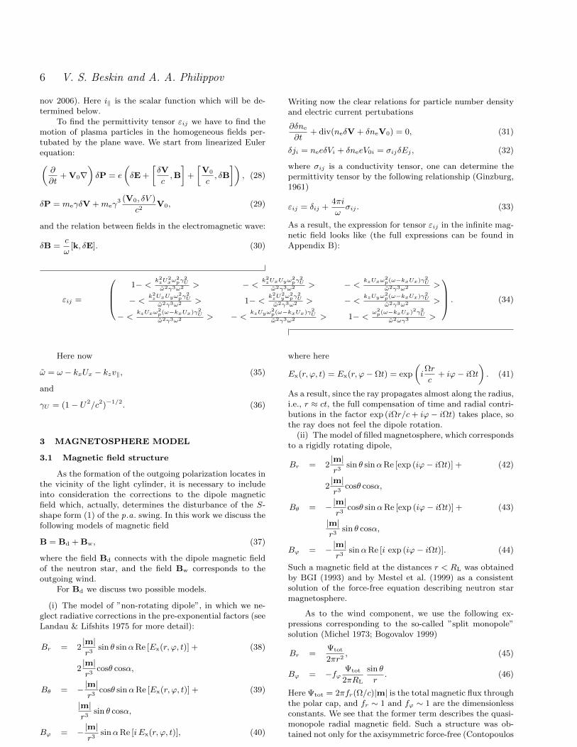
(i) The model of ”non-rotating dipole”, in which we ne-glect radiative corrections in the pre-exponential factors (seeLandau & Lifshits 1975 for more detail):

Br = 2|m|r3

sin θ sinαRe [Ex(r, ϕ, t)] + (38)

2|m|r3

cosθ cosα,

Bθ = −|m|r3

cosθ sinαRe [Ex(r, ϕ, t)] + (39)

|m|r3

sin θ cosα,

Bϕ = −|m|r3

sinαRe [i Ex(r, ϕ, t)], (40)

where here

Ex(r, ϕ, t) = Ex(r, ϕ− Ωt) = exp

(iΩr

c+ iϕ− iΩt

). (41)

As a result, since the ray propagates almost along the radius,i.e., r ≈ ct, the full compensation of time and radial contri-butions in the factor exp (iΩr/c+ iϕ− iΩt) takes place, sothe ray does not feel the dipole rotation.

(ii) The model of filled magnetosphere, which correspondsto a rigidly rotating dipole,

Br = 2|m|r3

sin θ sinαRe [exp (iϕ− iΩt)] + (42)

2|m|r3

cosθ cosα,

Bθ = −|m|r3

cosθ sinαRe [exp (iϕ− iΩt)] + (43)

|m|r3

sin θ cosα,

Bϕ = −|m|r3

sinαRe [i exp (iϕ− iΩt)]. (44)

Such a magnetic field at the distances r < RL was obtainedby BGI (1993) and by Mestel et al. (1999) as a consistentsolution of the force-free equation describing neutron starmagnetosphere.

As to the wind component, we use the following ex-pressions corresponding to the so-called ”split monopole”solution (Michel 1973; Bogovalov 1999)

Br =Ψtot

2πr2, (45)

Bϕ = −fϕΨtot

2πRL

sin θ

r. (46)

Here Ψtot = 2πfr(Ω/c)|m| is the total magnetic flux throughthe polar cap, and fr ∼ 1 and fϕ ∼ 1 are the dimensionlessconstants. We see that the former term describes the quasi-monopole radial magnetic field. Such a structure was ob-tained not only for the axisymmetric force-free (Contopoulos

c© 0000 RAS, MNRAS 000, 000–000


Table 1. Models of the magnetic field structure

model A B C

dipole i ii ii

wind fϕ = 0 fϕ = 0 fϕ = 1

et al. 1999; Timokhin 2006) and MHD (Komissarov 2006)numerical simulations but it describes well enough the mag-netic field of the inclined rotator as well (Spitkovsky 2006).As we are actually interested in the disturbance of the dipolemagnetic field inside the light cylinder only, we do not in-clude here into consideration the switching of the radial fieldin the current sheet in the equatorial region. As the totalmagnetic flux through the polar cap depends only weaklyon the inclination angle α (BGI; Spitkovsky 2006), we puthere for simplicity fr = 1 (for zero longitudinal current frchanges from 1.592 to 1.93).

Besides, the latter term Bϕ (46) corresponds to thetoroidal magnetic field connected with the longitudinal elec-tric current flowing in the magnetosphere. It is well-knownthat to support the MHD (in particular, force-free) outflowup to infinity the the total longitudinal current I is to beclose to the Michel (1973) current IM = ΩΨtot/4π (Con-topoulos et al. 1999). It corresponds to fϕ ≈ 1. On theother hand, for realizing this current for inclined rotatorwith dipole magnetic field, it is necessary to suppose that thecurrent density j‖ is much larger than the local Goldreich-Julian current jGJ ≈ ΩBcosα/2π (Beskin 2010). As it is notclear whether the Michel current IM > IGJ can be realizedin the pulsar magnetosphere, in what follows the parameterfϕ can be considered as a free one.

In Table 1 we present the notation of the models whichwill be used in what follows. Magnetic field structure formodel C (and for orthogonal rotator) is shown in Fig 5. Itis qualitatively similar to the numerical model obtained bySpitkovsky (2006).

3.2 Plasma number density

Recall the well-known property of the one-photon par-ticle production in a strong magnetic field: the secondaryparticles are produced only if the photon moves at largeenough angle to the magnetic field line (Sturrock 1971; Ru-derman & Sutherlend 1975; Arons & Scharlemann 1979).Since the relativistic particles near the neutron star surfacecan move only along the field lines with a Lorentz factorγ = (1 − v2‖/c

2)−1/2 (v‖ is the particle velocity along themagnetic field), the hard gamma-quanta emitted throughcurvature mechanism also begin to move along the field lines.As a result, the production of secondary particles will be su-pressed near the magnetic poles, where the magnetic fieldis nearly rectilinear. Therefore, one would expect the sec-ondary plasma density to be suppressed in the central regionof the open field lines (see Fig. 6). It is this property thatlies in the ground of the hollow cone model.

Bellow we assume that the plasma number density on apolar cap is known. It is convenient to rewrite it in the form

ne(θm, ϕm) = λg(θm, ϕm)n(0)GJ. (47)

Here n(0)GJ = ΩB/2πce is the amplitude of the Goldreich-

Figure 5. Structure of the magnetic field lines in equatorial planein corotating frame for the orthogonal rotator χ = 90. The mag-

netic field is considered as the sum of dipole and ”split-monopole”(model C). The scale corresponds to the light cylinder RL = c/Ω

Figure 6. Plasma space distribution function g(r⊥) on the polarcap as a function of the distance r⊥ from the magnetic axis for

f0 = 0.25. The dashed line corresponds to f0 = 0

Julian number density, i.e., it does not depend on theinclination angle α. Further, the multiplicity parameterλ = ne/n

(0)GJ determining the efficiency of the pair creation

is (Daugherty & Harding 1982; Gurevich & Istomin 1985;Istomin & Sobyanin 2009; Medin & Lai 2010)

λ ∼ 103 − 104. (48)

Finally, the dimensionless factor g(θm, ϕm) ∼ 1 describesthe real number density of the secondary plasma in the vicin-ity of the neutron star surface as a function of magnetic poleangles θm and ϕm.

The procedure described below allows us to determinethe properties of the outgoing radiation for arbitrary number

c© 0000 RAS, MNRAS 000, 000–000


density ne within the polar cap. For illustration we consideran axially symmetric distribution

g(f) =f2.5 exp(−f2)

f2.5 + f2.50

, (49)

where f = r2⊥/R20 is the dimensionless distance to the mag-

netic axis, R0 = (ΩR/c)1/2R is the polar cap radius, andthe parameter f0 describes the hole size in space plasmadistribution (see Fig. 6).

As was already stressed, in this paper we are going todiscuss the theoretical ground of propagation effects only.For this reason we assume here for simplicity the intensityof radio emission in the emission region to be proportionalto the number density of outgoing plasma. In reality thedirectivity pattern may differ drastically from the particleprofile.

To determine the number density ne of the outgoingplasma in the arbitrary point of the magnetosphere, we usequasi-stationary formalism, which is valid for quantities thatare functions of φ−Ωt. For such functions all time derivativescan be reduced to spatial derivatives by the following rules(Beskin 2009):

∂

∂tQ = −Ω

∂

∂φQ, (50)

1

c

∂

∂tV = ∇× [βR,V]− (∇V)βR, (51)

for any scalar (Q) and vector (V) functions. Here

βR =[Ω, r]

c. (52)

Using now the continuity equation

∂ne

∂t+ div(neV0) = 0, (53)

where the velocity V0 is given by Eqn. (27), one can obtain

(B∇)(nei‖) = 0. (54)

Hence, the product

nei‖ = const (55)

remains constant along the field lines (BGI, Gruzinov 2006).Taking now into account only the first order by Ωr/c andassuming that the velocity of the outflowing particles is closeto the light velocity c, we finally obtain

i‖ =1

B[1− (b, βR)]. (56)

Thus, to determine the number density ne at an arbi-trary point along the ray trajectory it is enough to know thenumber density and magnetic field B at the base of a givenfield line on the neutron star surface. But for this it is nec-essary to produce the back integration along the field linefrom any point along the trajectory up to the star surface.

In Fig. 7 we show the dependences of the distance of thefoot points to the magnetic axis r⊥ within the polar cap asa function of the distance r along the ray for rotating dipole(model B) and for magnetic field including the monopolewind (model C) for the phase point φ = −5. As for modelB the appropriate value can be obtained analytically (dashedcurve)

r⊥ = R

√R

rsinψm, (57)

Figure 7. Dependences of the distance of the foot points to the

magnetic axis within the polar cap as a function of the distance

r along the ray for rotating dipole (model B) and for magneticfield including the monopole wind (model C) for the phase point

φ = −5. Dashed curve corresponds to analytical expression (57)

where ψm is the angle between local point on the ray vectorand momentary magnetic axis, one can conclude that theprecision of our procedure is high enough.

3.3 Energy distribution and cyclotron absorption

As was shown by Andrianov & Beskin (2010), for largeenough shear of the magnetic field along the ray (as will beshown below, this condition does hold in the pulsar mag-netosphere), all the polarization characteristics of outgoingradiation depend on the diagonal components of dielectrictensor, that are not sensitive to the difference of the e+e−

distribution functions. This fundamental property allows usto consider the electron and positron energy distributionfunctions to be identical. Our particular choice is (see Fig. 8)

F (γ) =6γ0

21/6π

γ4

2γ6 + γ60

. (58)

This distribution has the maximum for γ = γ0 that isassumed as a typical Lorentz-factor of plasma particles,and has power-law spectrum γ−2 for large Lorentz-factorsγ γ0. Thus, it models well enough the energy distribu-tion function obtained numerically (Daugherty & Harding1982; BGI).

Finally, consider the cyclotron absorption taking placein the region where the condition ωB = γγU ω holds (seeAppendix B for more detail). As is well-known, the cyclotronresonance locates at the distances

rres ≈ 2 103Rν−1/3GHz γ

−1/3100 B

1/312 θ

−2/30.1 (59)

comparable with the escape radius resc (7) (Mikhailovskyet al. 1982). It implies that these two effects are to be con-sidered simultaneously. On the other hand, as was alreadystressed, in this region one can neglect the wave refraction,i.e., to put Re [n] = 1. Remember that the estimate (59) wasobtained for zero drift velocity U = 0. Nevertheless, as one

c© 0000 RAS, MNRAS 000, 000–000


Figure 8. Particle energy distribution function

Figure 9. Cyclotron resonance radius as a function of the pulsar

rotation phase for ν = 1GHz, γ0 = 100, and magnetic field modelB

can see on Fig. 9, the result of calculation for real case is inqualitative agreement with estimation (59)1.

As a result, the intensity of outgoing radiation can bedetermined as

I∞ = I0 exp(−τ), (60)

where I0 is the intensity in the emission region, and theoptical depth τ = 2ω/c

∫Im [n] dl can be found using the

clear relation

Im [n] ≈ Im [εy′y′ ]/2. (61)

As a result, we have

τ ≈ 4π2e2

mec

∞∫0

∞∫0

ne(l)ω

ωF (γ)δ

(|ωB |

√1− U2

c2− γω

)dγdl

=4π2e2

mec

∞∫0

ne(l)1

ωF

(|ωB |

√1− U2/c2

ω

)dl. (62)

1 Here the delta-function for particle energy distribution was as-

sumed, because in the case of distribution function (58) there is

the wide zone of cyclotron resonance.

Here we use the approximation v2‖/c2 ≈ 1 − U2/c2. In the

case of identical distribution functions for electrons andpositrons the difference in absorption of the O- and X-modesis proportional to τ∆N/N ≈ τ/λ, that is almost negligiblefor λ 1. It should be noted that the same result wasobtained by Wang et al (2010) using exact solution of theequations for the Stokes parameters near the cyclotron res-onance under the typical pulsar conditions. However, thisresult differs from one obtained by Petrova (2006).

Remember that for evaluation one can use the simplerelation (Mikhailovsky et al. 1982)

τ ≈ λ(1− cosθres)rresRL

. (63)

Hence, for rres ≈ 0.1RL, λ ≈ 104, and θres ≈ 0.1 the opticaldepth is to be high enough (τ ≈ 10). On the other hand, asshown on Fig. 6 and Fig. 7, for rres ≈ 0.1RL the ray passesthe very central parts of the open field lines region where theplasma number density ne can be much smaller than λnGJ

(g(f) 1). For this reason, as will be shown below, theabsorption of the outgoing radiation can be not so strong.

Finally, as it is shown on Fig. 9, in the case of rotatingmagnetosphere rres depends on the pulsar rotation phase.Competition of these two effects (i.e., non-uniform plasmadensity distribution and difference in cyclotron radii) deter-mines which part of the beam, leading or trailing one, willbe absorbed more efficiently.

4 LIMITING POLARIZATION

The limiting polarization effect is well-known(Zheleznyakov 1977). When the radiation escapes intothe region of rarefied plasma, the wave polarization ceasesto depend on the orientation of the external magneticfield. At the same time, in the domain of the dense enoughplasma where the geometrical optics approximation isvalid, the orientation of the polarization ellipse is to bedetermined by the direction of the external magnetic field.This implies that the geometrical optics approximationunder weak anisotropy conditions becomes inapplicableand the question about the pattern of the limiting polar-ization effect should be solved by using the equations thatdescribe a linear interaction of waves in an inhomogeneousmagnetoactive plasma.

Traditionally to describe general radiative transfer inmagnetoactive plasma four first-order differential equations(for all four Stokes parameters) are used (Sazonov 1969;Zheleznyakov 1996; Petrova & Lyubarskii 1990; Broderick& Blandford 2010; Wang et al. 2010; Shcherbakov & Huang2011). Budden eqution, i.e., the second-order equation to thecomplex function actually corresponds to the same approach(Budden 1972; Zheleznyakov 1977). On the other hand, boththe standard and the Zheleznyakov-Budden approaches arenot quite convenient for quantitative estimates of the polar-ization of the escaping emission in general case. But sincewe are going to describe the propagation of originally fullypolarized waves, not the ensemble of waves, we actually needonly two equations for observable parameters, i.e., the posi-tion angle and the Stokes parameter V .

There exists a different approach that allows us imme-diately write down the equations for these observable quan-tities, namely, the Stokes parameter V , defining the circular

c© 0000 RAS, MNRAS 000, 000–000


polarization and the position angle p.a., characterizing theorientation of polarization ellipse (Kravtsov & Orlov 1990).This approach is valid in the quasi-isotropic case, i.e., in thecase when the dielectric tensor can be presented as

εij = εδij + χij , (64)

where the anisotropic part χij is small as compared toisotropic one. In this case we have two small parameters— general WKB parameter 1/kL and

∆n/n1,2 ∼ χij/n1,2 1. (65)

As a result, the solution can be found by expansion over thistwo small parameters.

As one can check, these conditions are just realized inthe pulsar magnetosphere (Andrianov & Beskin 2010). In-deed, in the region r ∼ resc ∼ 103R the value of v = ω2

p/ω2

v ∼ 10−7 λ4B12 ν−2GHz P

−1, (66)

is much smaller than unity. Accordingly, the deviation of therefractive indices from unity, |n1,2−1| ∼ v, is also very smallhere, so we can neglect the wave refraction in the polariza-tion formation region.

The Kravtsov-Orlov equation

dΘ

dl= κ+

iω

4c[(χba − χab) + (χba + χab)cos2Θ−

(χaa − χbb) sin 2Θ], (67)

is the equation for the complex angle Θ = Θ1 + iΘ2, whereΘ1 is a position angle and Θ2 determines the circular polar-ization by the relation

V = I tanh2Θ2. (68)

Here I is the intensity of the wave. The components of thedielectric tensor χij are to be written in a frame of unitaryvectors a and b in the picture plane where a is determinedby the projection of the vector ∇ε. Finally,

κ = 1/2(a · [∇,a] + b · [∇,b]) (69)

is the ray torsion (see Kravtsov & Orlov 1990 for more de-tail). It can be easily understood that the rotation of positionangle described by the ray torsion is fictious and describesonly the rotation of coordinate system. As a result, we canwrite down

dΘ1

dl=

ω

2cIm [εx′y′ ]

−1

2

ω

cΛcos[2Θ1 − 2βB(l)− 2δ(l)]sinh2Θ2, (70)

dΘ2

dl=

1

2

ω

cΛ sin[2Θ1 − 2βB(l)− 2δ(l)]cosh2Θ2. (71)

Here l is a coordinate along the ray propagation, and theangle βB(l) defines the orientation of the external magneticfield in the picture plane (defined as tanβB = BY /BX ,where BX and BY are the components of the magnetic fieldvector in a XYZ system, see Fig. 3). Further,

Λ = ∓

√(Re [εx′y′ ])2 +

(εx′x′ − εy′y′

2

)2

, (72)

where the signs correspond to the regions before/after thecyclotron resonance and

tan(2δ) = − 2Re [εx′y′ ]

εy′y′ − εx′x′. (73)

Finally, εi′j′ are the components of plasma dielectric tensorin the frame where the z-axis directs along the wave prop-agation and the external magnetic field lies in the xz-plane(see Appendix C). As was already stressed, the singularitiesat the cyclotron resonance in equations (70)-(71) are absentdue to averaging over wide particle energy distribution. Fordistribution function (58) this averaging can be done ana-lytically.

We would like to note that in these equations the circu-lar polarization is defined as it is common in radio astronomy(positive V corresponds to LHC polarization). Nonrelativis-tic version of the above equations is given in Czyz et al.(2007). It should be mentioned that the equation for theStokes vector evolution has been recently shown to be de-rived directly from the Kravtsov-Orlov quasi-isotropic ap-proximation (Kravtsov & Bieg 2008).

As one can see on Fig. 10, in the geometrical opticsregion Eqns. (70)–(71) describe oscillations of the angle Θ1

near the value Θ1 = βB+δ. As the ray moves into the regionof rarefied plasma, the length of the spatial oscillations L ∼c/(ω∆n) increases and in the region r > resc becomes largerthan the characteristic length r. As a result, the angles Θ1

and Θ2 become constant for r resc. They are the valuesthat characterize the outgoing radiation.

Thus, the basic equations (70)-(71) generalize ones ob-tained by Andrianov & Beskin (2010) for zero drift velocityU = 0 when Re [εx′y′ ] = 0 and, hence, δ = 0. In particu-lar, they now include into consideration the aberration ef-fect considered by Blaskiewicz et al. (1991). This effect wasalso considered by Petrova & Lyubarskii (2000), but for theinfinite magnetic field only. It is important that in Eqns.(70)-(71) the angle Θ1 is measured relative to the labora-tory frame because these equations contain the differencebetween Θ1 and βB only.

Equations above have the following important property.For homogeneous media (βB = const, εij = const) the pa-rameters of polarization ellipse Θ1 and Θ2 remain constantif the following conditions are valid:

Θ1 = βB + δ, sinh2Θ2 =Im [εx′y′ ]

Λ= − 1

Q, (74)

Θ1 = βB + δ + π/2, sinh2Θ2 = − Im [εx′y′ ]

Λ=

1

Q. (75)

Here (see the definition of εi′j′ in Appendix D)

Q = iεy′y′ − εx′x′

2εx′y′. (76)

This closely corresponds to the polarization of the two nor-mal modes, the former corresponding to the O-mode, andthe latter to the X-mode. In addition, the following impor-tant property holds: irrespective of the pattern of changein plasma density and magnetic field along the trajectory,if two modes were orthogonally polarized in the beginning(Θ

(1)1 − Θ

(2)1 = π/2, Θ

(1)2 = −Θ

(2)2 ), then this property will

also be retain subsequently, including the region where thegeometrical optics approximation breaks down.

Finally, as was already mentioned, in the region r rescone can put dΘ1/dl ≈ d(βB + δ)/dl. Hence, for high enoughshear of the external magnetic field along the ray propaga-tion when the derivative d(βB + δ)/dx is high enough, thefirst term in the r.h.s. of Eqn. (70) may be neglected. As forΘ2 1 we have sinh2Θ2 ≈ tanh2Θ2, one can write down

c© 0000 RAS, MNRAS 000, 000–000


for V/I = tanh2Θ2

V

I≈ 1

|Q|d(βB + δ)/dx

A

1

cos[2Θ1 − 2βB(l)− 2δ(l)]. (77)

Here

A =∣∣v‖/c(1− sin θ Ux/c)− cosθ(1− U2/c2)

∣∣ , (78)

x = Ωl/c, and we used λnGJ for the plasma number density.Thus, the sign of the circular polarization will co-

incide with the sign of the derivative d(βB + δ)/dx forthe O-mode and they must be opposite for the X-mode.This approximation can be used for large enough deriva-tive d(βB + δ)/dx ∼ 1 (i.e., for large enough total turn∆(βB + δ) ∼ 1 within the light cylinder RL = c/Ω), andfor small angle of propagation θ 1 through the relativis-tic plasma (v‖/c ∼ 1). Both these conditions are valid inthe magnetospheres of radio pulsars with a good accuracy.Indeed, assuming that U/c 1 and Ux/c ≈ U/c ≈ θ onecan obtain

A ≈ θ2

2− 1

2γ2− Ux

csin θ +

U2

c2≈ θ2

2− 1

2γ2 1. (79)

So, the Stokes parameter V (77) is to be much larger thanV0 = ±I/Q resulting from standard evaluation (Ginzburg,1961).

It is important that in this case in the region where thegeometrical optics is valid the circular polarization is to bedetermined by the value of Λ (72) which does not depend onimaginary non-diagonal components of the dielectric tensorχab and χba. This fundamental property is well-known inplasma physics and crystal optics (see, e.g., Zheleznyakov etal. 1983; Czyz et al. 2007), but up to now it was not used inconnection with the pulsar radio emission. For radio pulsarsthis property is especially important because for electron-positron plasma the imaginary part of the dielectric tensordepends significantly on the difference in particle energy dis-tributions which is not known with the enough accuracy.

Finally, our numerical simulations show that the signof the derivative d(βB + δ)/dx is opposite to the sign ofdp.a./dφ. As one can see from Eqn. (77), this results in animportant prediction:

• For the X-mode the signs of the circular polarization Vand the derivative dp.a./dφ should be the SAME.• For the O-mode the signs of the circular polarization V

and the derivative dp.a./dφ should be OPPOSITE.

This implies also that the effects of the particle drift motion,as was already found by Blaskiewicz et al. (1991) (see alsoHibschman & Arons 2001), shifts the p.a. curve to the trail-ing part of the mean profile. As it is shown below, our resultsare in qualitative agreement with this statement. Moreover,at present there are some observational confirmations of thisproperty (Mitra & Rankin, 2011). Nevertheless, the maindistinction of our theory is in self-consistent definition ofresc (and, i.e., p.a. shift value) on the direct solution of po-larization transfer equations, that depends not only on thegeometry, but on plasma parameters as well.

Typical evolution of angles Θ1 and Θ2 are presented onFig. 10. It shows that the analytical estimate of the escaperadius (7) is qualitatively correct. Nevertheless, it shouldbe mentioned that it depends on the plasma multiplicityfactor, that depends effectively on pulsar rotation phase due

resc

resc

Figure 10. Evolution of the angles Θ1,2 for O-mode, φ = −5,λ = 103, γ0 = 50, ν = 1GHz, and magnetic field model B. Their

small oscillations in the region r resc can be seen for Θ2 onlydue to the different scales in the upper and lower panels. The dash

lines correspond to the geometrical optics values Θ1 = βB+δ and

Θ2 = 1/2Q

to non-uniform plasma number density distribution. It alsoshows that real values of Θ2 are indeed much larger thanthe corresponding standard value 1/2Q.

5 RESULTS

Thus, in this paper the arbitrary non-dipole magneticfield configuration, arbitrary number density profile withinthe polar cap, the drift motion of plasma particles, and theirrealistic energy distribution function are taken into account.It gives us the first opportunity to provide the quantitativecomparison of the theoretical predictions with observationaldata. Using numerical integration we can now model themean profiles of radio pulsars and, hence, evaluate the phys-ical parameters of the plasma flowing in the pulsar magne-tosphere.

It is necessary to stress that the detailed discussion ofthe morphological properties of mean profiles resulting fromdifferent inclination and impact angles is beyond the scope ofour consideration and are addressed to future papers. Thegoal of this paper is in quantitative analysis of the prop-agation effects on the polarization characteristics of radiopulsars. In particular, we try to determine how the plasma

c© 0000 RAS, MNRAS 000, 000–000


Table 2. Parameters of the ’ordinary’ pulsar

P B0 α β f0 rem γ0 λ

1 s 1012 G 45 −3 0.25 30R 50 103

parameters affect the S-shape of the position angle swingand the properties of the mean profile.

5.1 Ordinary pulsars

At first, let us discuss the results obtained by numeri-cal integration of equations (70)–(71) for ”ordinary” pulsar(its parameters are given in Table 2). Everywhere below thedashed curves on the intensity panel show the intensity pro-file without any absorption. As was already stressed, in thispaper for simplicity we suppose that it repeats the particlenumber density profile shown in Fig. 6. If the dashed curveis not shown, then the absorption is fatal and only the origi-nal intensity (which is normalized to 100 in its maximum) isshown. The dashed curves on p.a. panels show the predictionof the RVM-model (1). Finally, pulsar phase φ is measuredin degrees everywhere below.

On Fig. 11 we show the intensity I∞ (60) (left panel)and the p.a. swing (right panel) for extraordinary X-mode asa function of the pulsar phase φ for ”non-rotating dipole”without the wind component (model A); the drift effectsare neglected as well. The circular polarization degree doesnot exceed one percent here and that is why this curve isnot presented in this picture. It results from approximatelyconstant βB along the ray. For this reason, as we see, thep.a. curve is nicely fitting by the RVM model.

Further, the upper solid line corresponds to f0 = 0.25,and the lower one corresponds to f0 = 0.0025. The lowerintensity curve shows that for the very small core in thenumber density f0 = 0.0025 (r⊥/R0 = 0.05) the absorptionis fatal and the emission cannot escape from the magneto-sphere. As was already stressed, this property can be eas-ily explained. Indeed, for f0 1 the rarefied region of the”hollow cone” is actually absent, and the rays pass the cy-clotron resonance in the region of rather dense plasma. Onthe other hand, for f0 ≈ 1 the number density in the regionof the cyclotron resonance is low enough for rays to escapethe magnetosphere without strong absorption.

Below we consider model C as the main magnetic fieldmodel of our simulation. As to model B, one can find theexamples of mean profiles basing on this model in Wang etal. (2010). The main differences between our results and onespresented in the paper mentioned above are in shifting of thep.a. curve to the trailing part (because of the particle driftmotion) and in possibility of absorption of the leading partof the pulse (due to the non-zero toroidal magnetic field).

On Fig. 12 we show the p.a. swing (lower panels), theintensity I∞ (solid lines on the top panels), and the Stokesparameter V (dotted lines) as a function of the pulsar phaseφ for extraordinary wave for magnetic field model C andfor various multiplicity parameter λ. It is obvious that theabsorption increases with increasing λ. In most cases, thetrailing part of the mean profile is absorbed (see Dyks et al.2010 as well).

Besides, as one can see, the p.a. curves differ signifi-

cantly from the RVM one (dashed lines) as λ growing. Thisproperty can be easily understood as well. Indeed, as theescape radius resc (7) increases as λ2/5, for large enough λthe polarization properties of the outgoing waves are to beformed in the vicinity of the light cylinder, i.e., in the regionwith quasi-homogeneous magnetic field (see Fig. 5).

Further, as was already mentioned, the drift effectcauses the p.a. curve to be shifted to the trailing part of themean profile. It is necessary to stress that the opposite shiftis to take place if we neglect the drift effect on the dielectrictensor (Andrianov & Beskin 2010; Wang et al. 2010). Onecan note that for high values of multiplicity parameter (i.e.,for full absorption of the trailing part of the mean pulse) theobserver will detect approximately constant p.a. Finally, asone can see from Eqn. (78), the maximum of circular polar-ization is also shifted to the trailing side, as larger devia-tions from the S-shape produce larger circular polarization.It is not visible on this picture because the trailing side ofthe beam is absorbed. Thus, one can conclude that the self-consistent quantitative analysis of observational data is toinclude these effects into consideration.

Another point should be mentioned. It is known thatcorrect accounting of the inverse Compton scattering of thesurface X-rays can reduce the pair multiplicity significantly(see, e.g., Hibschman & Arons 2001). In this case plasmaseffects on emission polarization can be negligible.

On Fig. 13 we show the same dependences for variousLorentz-factors of outgoing plasma γ0 = 10, 50, and 300. Asthe escape radius resc (7) decreases as γ−6/5, the largest shiftof the p.a. curve takes place for small γ0 = 10. Finally, onFig. 14 one can see the same dependences for various wavefrequencies ν = 0.03, 0.2, and 0.5 GHz. As resc ∝ ν−2/5, thelargest shift of the p.a. curve takes place for small frequen-cies. One can note that the full investigation of frequencydependence of mean profiles of radio pulsars is more com-plicate and must include, e.g., the detailed analysis of fre-quency dependence of the emission radius rem (BGI). Thisis beyond the scope of the article.

As was demonstrated above, in general the sign of thecircular polarization remains constant for a given mode. Butunder certain conditions the change of the V sign in the samemode may occur. It can take place when we cross the direc-tivity pattern in the very vicinity of the magnetic axis. Suchan example for the X-mode is shown on Fig. 15 for P = 1s,ζ = 49, α = 48.5, λ = 103, γ0 = 50, and rem = 100R.Certainly, this example is illustrative only. To explain thechange of the sign of the circular polarization in the centreof the mean profile the separate consideration is necessary.

Finally, in Table 3 we present the values of maximumderivative (dp.a./dφ)max, that is commonly used for deter-mination of the inclination angle α (see, e.g., Kuzmin &Dagkesamanskaya 1983; Malov 1990; Everett & Weisberg2001). As we see, these values significantly depend on theplasma parameters (and can differ drastically from the RVMvalue). Hence, more precise specifying of magnetosphericand plasma model is necessary for quantitative analysis ofthe pulsar characteristics.

In our opinion, this technique can be applied in futurefor radio pulsars for which the whole S-swing is detected.Otherwise, the situation like in Fig. 12 for λ = 104 mayoccur, when one can detect only constant part of the p.a.swing. At any way, one can conclude that if one try to fit

c© 0000 RAS, MNRAS 000, 000–000


-10 -5 0 5 10

0

20

40

60

80

100

Φ

I

-10 -5 0 5 10

40

60

80

100

120

140

Φ

p.a.

Figure 11. The intensity I∞ (60) (left panel) and the p.a. swing (right panel) as functions of the pulsar phase φ (in degrees) for ”non-rotating dipole” (model A). Here and below the dashed curves on the intensity panel show the intensity profile without any absorption.

The upper solid line corresponds to f0 = 0.25, and the lower one – to f0 = 0.0025

the whole p.a. curve by the RVM function (1), then for lowenough number density (λ < 104) and high enough particleenergy (γ0 > 50) the angles α and β obtained will satisfy thereality. But in other cases unexpected result may occur. Asshown on Fig. 16, left panel (see Table 2 as well), the sim-ulated curve could be nicely fitted by the RVM model withnon-zero shift value (1), but with the angles β ≈ −5 andα ≈ 97 that drastically differ from real ones α = 45 andβ = −3. On the other hand, the precision in determinationof the angles α and β may be not so high (see Fig. 16, rightpanel).

5.2 Two modes profiles

On Fig. 17 an examples of the mean profiles includingtwo orthogonal modes are presented. The ratio of the inten-sities in the radiation domain r = rem was assumed to beI(0)O /I

(0)X = 1/3. The jumps in the p.a. curves were done at

the phase φ where IO = IX. As we see, this jump can dif-fer from 90. This results from the different trajectories oftwo orthogonal modes. It is necessary to stress that in ourconsideration the ratio I

(0)O /I

(0)X is free, and its precise de-

termination is a question for the radio emission generationtheory.

We see that for radio pulsars for which two modes canbe observed the mean profiles are indeed to have the tripleform, which, in general, are not to be symmetric. As theO-mode deviates from magnetic axis, we have to see the O-mode in the leading part, the X-mode in the centre, andagain the O-mode in the trailing part of the mean profile.The detailed comparison with observational data will be pre-pared in the separate paper.

5.3 Millisecond pulsars

As the last example, on Fig. 18 we show the meanprofiles obtained for millisecond pulsar (the parameters aregiven in Table 4). One important feature appearing here isthat the leading, not trailing part of the mean profile can beabsorbed. It is caused by the bending of the open field linestube near the light cylinder due to non-dipolar magnetic

Table 4. Parameters of the millisecond pulsar

P B0 α β f0 rem γ0 λ

20 ms 108 G 45 −3 0.04 1.25R 50 103

field. As a result, the cyclotron resonance takes place in theregion of rarefired plasma for the trailing part of the pulse.Also, stronger deviations from the S-shape of p.a. swing arefound as compared to the case of ordinary pulsar, becausethe polarization forms closer to the light cylinder.

6 DISCUSSION AND CONCLUSIONS

In this paper we study the influence of the propagationeffects on the mean profiles of radio pulsars. The Kravtsov-Orlov approach allows us firstly to include into considera-tion the transition from geometrical optics to vacuum prop-agation, the cyclotron absorption, and the wave refractionsimultaneously. Arbitrary non-dipole magnetic field config-uration, drift motion of plasma particles, and their realisticenergy distribution were taken into account. Using numer-ical integration, we found how the propagation effects cancorrect the main characteristics of the hollow cone model.

To summarize, one can formulate the following results:

• We confirm the one-to-one correlation between the signsof circular polarization V and the position angle derivative(dp.a./dφ) along the profile for both ordinary and extraordi-nary waves. For the X-mode the signs should be the SAME,and OPPOSITE for the O-mode.• The standard S-shape form of the p.a. swing (1) can

be realized for small enough multiplicity λ and large enoughbulk Lorentz-factor γ only. In other cases the significant dif-ferences can take place. The location of the p.a. maximumderivative (dp.a./dφ)max is shifted to the trailing side of thepulse.• The value of p.a. maximum derivative (dp.a./dφ)max,

that is often used for determination the angle between mag-netic dipole and rotation axis, depends on the plasma pa-rameters [and differs from rotation vector model (RVM)

c© 0000 RAS, MNRAS 000, 000–000


Figure 12. The same for model C and for different multiplicity factors λ = 102, 103, 104, and 105. Here γ0 = 50 and ν = 1GHz. Dottedlines correspond to Stokes parameter V

c© 0000 RAS, MNRAS 000, 000–000


Figure 13. The same for various Lorentz-factors γ0 = 10, 50, and 300. Here λ = 103, and ν = 1GHz

value] and, hence, cannot be used without more precise spec-ifying of magnetospheric plasma model.• In general, the trailing side of the emission beam is

absorbed.

In our opinion, even the preliminary considerationdemonstrates that these conclusions are not in contradic-tion with observational data. The first statement is in goodagreement with observations (Han et al. 1998; Andrianov &Beskin 2010). In some cases, the sign reversal in the core canoccur (see Fig. 15 and Wang et al. 2010), that is detectedfor several pulsars (see also Radhakrishnan & Rankin 1990).The second point is in agreement with empirical model ofBlaskiewicz et al. (1991). On the other hand, as the shiftvalue depends on plasma parameters (assuming fixed geom-etry), the solution of the inverse problem (i.e., the fitting of

the real pulsar profiles) can in principle provide us a chanceof correct enough estimating of plasma parameters. Finally,the last point is in agreement with observations as well (see,e.g., Backus et el., 2010). In more detail, it takes place forlarge enough multiplicity parameter λ > 103. But in somecases the leading part can be absorbed as well. It happenswhen the polarization forms close to the light cylinder.

Finally, Fig. 19 demonstrates our understanding of theX- and O-modes propagation in the pulsar magnetosphere.Here the dot-dash lines going to the panels with pulsar pro-files show different intersections of directivity pattern, thatform the observable profiles. Resulting from the differentpropagation, the O- and X-modes produce two concentriccones, the inner (core) part corresponding to the X-modeand the outer (conal) one to the O-mode. Remember that

c© 0000 RAS, MNRAS 000, 000–000


Figure 14. The same for model C and for various frequencies ν = 0.03, 0.2, and 0.5 GHz. Here λ = 103, and γ0 = 50

the analysis of the relative intensity in O- and X-modes is aquestion for generation theory. In the context of the presentpropagation theory this parameter should be considered asa free one.

Another source of uncertainty which can affect the for-mation of the mean profile (and, in particular, results inthe formation of its more complicated shape) is the possi-ble ”spotty” of the directivity pattern, i.e., the presence ofthe separate radiative domains within the diagram (Rankin1993). As is well-known, such separate domains are observedas a subpulse drift (Ruderman & Sutherland 1975, Desh-pande & Rankin 2001).

In addition, the full analysis is to include the possiblelinear depolarization. E.g., depolarization at the edges ofthe profile can be easily interpreted as a mixing of X and

O-modes (Rankin & Ramachandran 2003). But the totaldegree of linear polarization (e.g., if we clearly see only onemode) is a question to propagation in the generation region.If this region is rather thick then one can expect the possibledepolarization. For this reason we do not treat here the totaldegree of linear polarization at all.

As we see, in general if only one mode dominates inpulsar profile, then we expect statistically D (double) meanprofile for the O-mode and S (single) one for the X-mode. Ofcourse, we suppose here that there is nonzero natural widthof the radiative domains that efficiently smooths the hollowcone corresponding to the narrow X-mode. Nevertheless, asis shown on Fig. 19, the X-mode can in principal produce Dprofile and O-mode can produce S ones. The XD and XSprofiles can be obtained when only X-mode is produced in

c© 0000 RAS, MNRAS 000, 000–000


-15 -10 -5 0 5 10 15

0

20

40

60

80

100

Φ

I,V

-15 -10 -5 0 5 10 15

50

100

150

Φ

p.a.

Figure 15. The results of simulations for X-mode, P = 1s, β = −0.5, α = 48.5, λ = 103, γ0 = 50, and rem = 100R. It shows thatunder certain conditions the change of V sign in the same mode may occur

Figure 16. The left panel shows the p.a. swing (points) for γ0 = 50, λ = 105, ν = 1GHz, α = 45, and β = −3. Solid line correspondsto the best RVM fit giving unrealistic values α = 97 and β = −5. The right panel shows χ2 map for RVM fitting

Table 3. The position angle maximum derivative (dp.a./dφ)max and the shift ∆φ of its position

λ γ0 ν (GHz) (dp.a./dφ)max RVM ∆φ()

102 50 1 −9.47 −10.14 4.7

104 50 1 −14.47 −10.14 7.4

105 50 1 −11.70 −10.14 10.5

103 10 1 −12.72 −10.14 11.5

103 50 1 −9.86 −10.14 4.3

103 100 1 −9.47 −10.14 4.7

103 300 1 −9.46 −10.14 4.0

103 50 0.03 −15.92 −10.14 8.4

103 50 0.5 −11.82 −10.14 3.8

103 50 0.2 −18.02 −10.14 5.5

c© 0000 RAS, MNRAS 000, 000–000


0 0

Figure 17. Main profiles including both modes (O and X ones) for λ = 103 and 104. Here γ0 = 50, and ν = 1GHz

the formation region. On the other hand, if there are twomodes with the similar intensity, the triple (T) and mul-tiple (M) profiles can be obtained as well. So, this pictureis in agreement with Rankin’s morphological classification(Rankin 1983). Our investigation provides an additional in-formation to morphological structure, i.e., the informationof the type of the mode that forms mainly the mean pro-file. As was demonstrated, only the correlation between p.a.derivative and V signs provides us this chance.

Finally, the determination of the angular dimension ofthe core and conal beams depends greatly on the emissionradius (i.e., again, on the generation mechanism). So the de-tailed analysis is also beyond the scope of current investiga-tion (one can find empirical results on this in, e.g., Maciesiak& Gil 2011).

Thus, the approach developed in this paper allows thepredictions of the theory of radio emission to be quanti-tatively compared with the observational data. Moreover,based on the observational data, one can reject a numberof models in which the shapes of the profiles of the positionangle and the degree of circular polarization never realizedin practice are obtained. Thus, it becomes possible to solvethe inverse problem, i.e., to determine the parameters of theoutflowing plasma and the magnetic field structure.

We will be glad to any collaboration with observers forinvestigating the observational features of the mean profileson the base of our theory. The source code of our calculations(in Mathematica 7 or C) is available under request.

7 ACKNOWLEDGMENTS

We thank Prof. A.V. Gurevich and Ya.N. Istominfor his interest and support, and J. Dyks, A. Jessner, P.Jaroenjittichai, M. Kramer, V.V. Kocharovsky, D. Mitra,M.V. Popov, R. Shcherbakov, B. Rudak, and H.-G. Wangfor useful discussions. We also thank A. Spitkovsky for valu-able opportunity and assistance in dealing with his numeri-cal solution and for outstanding discussions. This work waspartially supported by Russian Foundation for Basic Re-search (Grant no. 11-02-01021).

APPENDIX A: REFRACTION

In this work we consider the simple model of the refrac-tion obtained under the assumption that the plasma numberdensity is constant within the polar cap, i.e., g(θm, ϕm) = 1.To include refraction into consideration we introduce the”imaginary source” of radiation giving the same trajectoryat large distances whence emitted parallel to the magneticfield line (see Fig. A1). As the ”tearing off” level locatesdeeply in the magnetosphere, i.e., rA RL, one can use theanalytical expression (22) for the angle θ⊥∞ (BGI 1993). Itgives for the polar angle of the emission point

θem ≈

[(lrR

)0.21

θ⊥∞

(1

ω2

⟨ω2p0

γ3

⟩)−0.07]1.39

(A1)

(for dipole magnetic field it does not depend on the radialdistance). As a result, we obtain for the polar angle of imag-inary source

c© 0000 RAS, MNRAS 000, 000–000


Figure 18. The results of simulations for X-mode for the millisecond pulsar for multiplicity parameters λ = 102 (left panel) and λ = 103

(rigth panel)

Figure A1. Imaginary source corresponding to rectilinear prop-agation of the wave

tan θim =4

3

tan θ⊥∞

1 +√

1 + 8/9 tan2 θ⊥∞. (A2)

After some algebraic calculations, one can find the trajectory

R = m(φ)ρcosθim + m⊥(φ)ρ sin θim + rez.

Here

ρ(φ) = lt| sinβ − cosβ tan θ⊥∞)|| tan θim − tan θ⊥∞|

√1 + tan2 θim (A3)

is the radius of imaginary source, and

β =Ψ

2+

1

2arcsin

(sin Ψ

3

), (A4)

where

Ψ = θ⊥∞ −

[1

ω2<ω2p0

γ3>

(ltR

)−3]1/4

. (A5)

Finally, m⊥(φ) is a unit vector perpendicular to m(φ) lyingfor every pulsar phase φ in the plane containing the magneticm(φ) and the wave k vectors.

APPENDIX B: DERIVATION OF DIELECTRICTENSOR

Since all the quantities in equation (28) are proportionalto exp (−iωt+ ikr), its solution can be easily obtained:

δvx =1

ω2B − γ2γ2

U ω2

[−iωγ

(1 + γ2

U

U2y

c2

)D1 +

(ωB + iωγγ2

UUxUyc2

)D2

], (B1)

c© 0000 RAS, MNRAS 000, 000–000


Figure 19. Formation of the directivity pattern in the pulsar magnetosphere. The X-mode propagating rectilinearly forms the corecomponent, and deflected from the magnetic axis O-mode forms the conal one. The lower curves on each top panels indicate the Stokes

parameter V , and the bottom panels shows the p.a. swing. Corresponding pulsar profiles was taken from Weltevrede & Johnston (2008)

δvy =1

ω2B − γ2γ2

U ω2

[−iωγ

(1 + γ2

UU2x

c2

)D2 +

(−ωB + iωγγ2

UUxUyc2

)D1

], (B2)

δvz = ieγ2U

meωωγ3[ωδEz + kz(V0, δE)]−

v‖c2γ2U (Uxδvx + Uyδvy), (B3)

where

D1 =e

meω

[ωδEx + kx(V0, δE)− γ2

U

Uxv‖c2

(ωδEz + kz(V0, δE))

], (B4)

D2 =e

meω

[ωδEy − γ2

U

Uyv‖c2

[ωδEz + kz(V0, δE)]

]. (B5)

From (31) one can find the number density pertubation

δne =ne

ω(k, δv) . (B6)

After making substitution to (32) we obtain for dielectrictensor components:

εxx = 1− <γ2Uk

2zU

2xω

2p

ω2γ3ω2> + <

ω2p[ω2

0 + U2x/c

2(γ2Uk

2zv

2‖ − ω2)]γγ2

U

ω2(ω2B − γ2γ2

U ω2)

>, (B7)

c© 0000 RAS, MNRAS 000, 000–000


εxy = − <γ2Uk

2zUxUyω

2p

ω2γ3ω2> +i <

γ2Uω

2pωB(ω0 − ωU2/c2)

ω2[ω2B − γ2γ2

U ω2]

> + <ω2p[ω0kxUy + UxUy/c

2(γ2Uk

2zv

2‖ − ω2)]γγ2

U

ω2(ω2B − γ2γ2

U ω2)

>, (B8)

εxz = − <γ2UkzUxω

2p(ω − kxUx)

ω2γ3ω2> + <

ω2p[(ω0 − ωU2/c2)v‖(kx − ωUx/c2) + kzkxv

2‖U

2y/c

2]γγ4U

ω2(ω2B − γ2γ2

U ω2)

>

−i <γ2UωBω

2p

ω(ω2B − γ2γ2

U ω2)

Uxv‖c2

>, (B9)

εyy = 1− <k2zγ

2UU

2yω

2p

ω2γ3ω2> + <

ω2p[ω2 + U2

y/c2(k2zv

2‖γ

2U − ω2) + k2xU

2y ]γγ2

U

ω2(ω2B − γ2γ2

U ω2)

>, (B10)

εyz = − <kzUyγ

2Uω

2p(ω − kxUx)

ω2γ3ω2> + <

ω2p[k2xc

2 − ω2 + γ2Ukzv‖(ω − kxUx)]γ

ω2(ω2B − γ2γ2

U ω2)

Uyv‖γ2U

c2>

−i <ωBω

2pγ

2U

ω2(ω2B − γ2γ2

U ω2)v‖(kx −

ωUxc2

) >, (B11)

εzz = 1− <ω2p(ω − kxUx)2γ2

U

ω2ω2γ3> + <

ω2p[(kxc− ωUx/c)2 + U2

y/c2(ω2 − k2xc2)]γ

ω2(ω2B − γ2

Uγ2ω2)

v2‖γ4U

c2>, (B12)

Im [εyy] = −π <ω2p[ω2 + U2

y/c2(k2zv

2‖γ

2U − ω2) + k2xU

2y ]γU

ω2ωδ(|ωB | − γγU ω) > . (B13)

c© 0000 RAS, MNRAS 000, 000–000


Here the quantity ω0 = ω− kzv‖. Other components ofthe permittivity tensor are defined by its hermiticity. There-fore, in the expression for gyrofrequency

ωB =eB

mec

we should take into the account the sign of the charge e. One

can check that moving to the appropriate reference framethis dielectric tesor reduces to the well-known one (Godfrayet al. 1975; Suvorov & Chugunov 1975; Hardee & Rose 1975)obtained for the case E = 0. Finally, as we see, the cyclotronresonance corresponds to the condition ωB = γγU ω.

As a result, one can find for the coefficients in Kravtsov-Orlov equations (70)–(71):

Λ = −1

2<

ω2p

ω2γ3

γ2Uω

2B

ω2B − γ2γ2

U ω2>[(sin θ − Ux/c)2 + cos2θ U2

y/c2] , (B14)

Re [εx′y′ ] = <ω2p

ω2γ3

γ2Uω

2B

ω2B − γ2γ2

U ω2> Uy/c (sin θ − Ux/c) cosθ, (B15)

εy′y′ − εx′x′ = <ω2p

ω2γ3

γ2Uω

2B

ω2B − γ2γ2

U ω2>[(sin θ − Ux/c)2 − cos2θ U2

y/c2] , (B16)

Im [εx′y′ ] = <ω2p

ω

γ2UωB

ω2B − γ2γ2

U ω2>[cosθγ−2

U − v‖/c(1− sin θ Ux/c)], (B17)

tan(2δ) = − 2Uy/c cosθ(sin θ − Ux/c)(sin θ − Ux/c)2 − cos2θU2

y/c2, (B18)

tan(δ) = − cosθ Uy/c

sin θ − Ux/c. (B19)

APPENDIX C: ROTATION OF COORDINATESYSTEMS

The equations of the transition of the dielectric tensorfrom the coordinate system formulated in Sect. 3 to thatused in Sect. 4 are the following

εx′x′ = εxxcos2θ + εzz sin2 θ − (εxz + εzx) sin θ cosθ,

εy′y′ = εyy,

εz′z′ = εxx sin2 θ + εzzcos2θ + (εxz + εzx) sin θ cosθ,

εx′y′ = εxycosθ − εzy sin θ,

εy′z′ = εyx sin θ + εyzcosθ,

εx′z′ = (εxx − εzz) sin θ cosθ + εxzcos2θ − εzx sin2 θ.

Here θ is the angle between the ray propagation and localmagnetic field directions. Other components of the tensorcan be defined by its hermiticity.

APPENDIX D: NATURAL MODES

For obtaining naturals modes of tensor εi′j′ it is con-venient to rotate the coordinate frame in xy-plane to makethe condition Re [εx′y′ ] = 0 to be valid. One can find that itcan be done by rotation defined by the following matrix:

M =

cosa − sin a 0sin a cosa 0

0 0 1

, (D1)

where

tan(2a) = tan(2δ) = − 2Re [εx′y′ ]

εy′y′ − εx′x′. (D2)

In this frame the corresponding expressions for tensor com-ponents (defining as εi′j′) are:

εx′x′ = εx′x′cos2a+ εy′y′ sin2 a+ 2Re [εx′y′ ] sin a cosa,

εy′y′ = εx′x′ sin2 a+ εy′y′cos2a− 2Re [εx′y′ ] sin a cosa,

εx′y′ = i Im [εxy].

The naturals modes for this tensor (with pure imaginaryx’y’ component) are well-known (Andrianov & Beskin 2010;Wang et al. 2010):

Θ1 = β, sinh2Θ2 = − 1

Q, (D3)

Θ1 = β + π/2, sinh2Θ2 =1

Q, (D4)

where by the definition

Q = iεy′y′ − εx′x′

2εx′y′. (D5)

It can be easily shown that in our case

1

Q= − Im [εx′y′ ]

Λ. (D6)

Hence, Eqns. (74)-(75) really define the natural modes in thelaboratory frame. The simple expression, which correspondsto a zero plasma temperature for Q is the following (cf.Melrose & Luo 2004 for zero drift):

Q =λωBω

[(sin θ − Ux/c)2 + U2

y/c2cos2θ

]2γ3ω2

[cosθ(1− U2/c2)− v‖/c(1− sin θ Ux/c)

] . (D7)

REFERENCES

Andrianov A.S., Beskin V.S., 2010, Astron. Lett., 36, 248Arons J., Scharlemann E.T., 1979, Astrophys. J., 231, 854

c© 0000 RAS, MNRAS 000, 000–000


Asseo E., 1995, MNRAS, 276, 74Asseo E., Pellat R., Rosado M., 1980, Astrophys. J., 239,661

Backus I., Mitra D., Rankin J., 2010, MNRAS, 404, 30Barnard J.J., 1986, Astrophys. J., 303, 280Barnard J.J., Arons J., 1986, Astrophys. J., 302, 138Beskin V.S., 1999, Physics-Uspekhi, 169, 1169Beskin V.S., 2009, MHD Flows in Compact AstrophysicalObjects, Springer, Berlin

Beskin V.S., 2010, Physics-Uspekhi, 180, 1241Beskin V.S., Gurevich A.V., Istomin Y.N., 1988, Astro-phys. and Space Sci., 146, 205

Beskin V.S., Gurevich A.V., Istomin Y.N., 1993, Physics ofthe Pulsar Magnetosphere, Cambridge University Press,Cambridge (BGI)

Blandford R.D., 1975, MNRAS, 170, 551Blaskiewicz M., Cordes J.M., & Wasserman I, 1991, Astro-phys. J., 370, 643

Bogovalov S.V., 1999, Astron. Astrophys., 349, 1017Broderick A.E., Blandford R.D., 2010, ApJ, 718, 1085Budden K.G., 1972, J. Atm. Terr. Phys., 34, 1909Cheng A.F., Ruderman M.A., 1979, Astrophys. J., 229, 348Contopoulos I., Kazanas D., Fendt Ch., 1999, Astrophys.J., 511, 35

Czyz Z.H., Bieg B., Kravtsov Yu.A., 2007, Phys. Lett. A,368, 101

Daugherty J.K., Harding A.K., 1982, Astrophys. J, 252,337

Deshpande A.A., Rankin J., 2001, MNRAS, 322, 438Dyks J., Wright G.A.E., Demorest P.B., 2010, MNRAS,405, 509

Everett J.E., Weisberg J.M., 2001, ApJ, 553, 341Fussel D., Luo Q., Melrose D.B., 2003, MNRAS, 343, 1248Ginzburg V.L., 1961, Propagation of ElectromagneticWaves in Plasma, Gordon & Breach Science Publishers,New York

Godfray B.B., Shanahan W.R., Thode L.E., 1975, Phys.Fluids, 18, 346

Goldreich P., Keeley D.A., 1971, Astrophys. J., 170, 463Gruzinov A., 2006, ApJ, 647, 119Gurevich A.V., Istomin Y.N., 1985, Sov. Phys. JETP, 62,1

Hankins T.H., Rankin J.M., 2010, AJ, 139, 168Han J., Manchester R., Xu R., Qiao G., 1998, MNRAS,352, 915

Hardee Ph.D., Rose W.K., 1975, Astrophys. J., 210, 533Hibschman J.A., Arons J., 2001, Astrophys. J., 546, 382Istomin Y.N., 1988, Sov. Phys. JETP, 67, 1380Istomin Y.N., Sobyanin D.N., 2009, Phys. JETP, 109, 393Kazbegi A.Z., Machabeli G.Z., Melikidze, G. I., 1991, MN-RAS, 253, 377

Keith M. J., Johnston S., Weltevrede P., Kramer M., 2010,MNRAS, 402, 745

Kravtsov Yu.A., Bieg B., 2008, Cent. Eur. J. Phys., 6, 563Kravtsov Yu.A., Orlov Yu.I., 1990, Geometrical Optics ofInhomogeneous Media, Springer, Berlin

Kuzmin A. D., Dagkesamanskaya I. M., 1983, Sov. As-tron.Lett., 9, 80

Landau L.D., Lifshits E.M., 1975, The Classical Theory ofFields, Pergamon Press, Oxford

Luo Q., Melrose D.B., Machabeli G. Z., 1994, MNRAS,268, 159

Lyubarskii Yu.E., 1996, Astron. Astrophys., 308, 809

Lyubarskii Yu.E., 2008, AIP Conference Proceedings, 983,29-37

Lyne A.G., Graham-Smith F., 1998, Pulsar Astronomy,Cambridge University Press

Maciesiak K., Gil J., 2011, MNRAS, 417, 1444

Malov I.F., 1990, Sov. Astron., 34, 189

Manchester R., Taylor J., 1977, Pulsars, Freeman, SanFrancisco

Medin Z., Lai D., 2010, MNRAS, 406, 1379

Melrose D.B., Luo Q., 2004, MNRAS, 352, 915

Michel F.C., 1973, Astrophys. J., 180, L133

Mikhailovsky A.B., Onishchenko O.G., Suramlioshvili G.I.,Sharapov S.E., 1982, Sov. Astron. Lett., 8, 685

Mitra D., Gil J., Melikidze G., 2009, Astrophys. J., 696, 2

Mitra D., Rankin J., 2011, Astrophys. J., 727, 92

Petrova S.A., 2001, Astron. Astrophys. 378, 883

Petrova S.A., 2003, Astron. Astrophys. 408, 1057

Petrova S.A., 2006, MNRAS 368, 1764

Petrova S.A., Lyubarskii Yu.E., 1998, Astron. Astrophys.,333, 181

Petrova S.A., Lyubarskii Yu.E., 2000, Astron. Astrophys.,355, 1168

Radhakrishnan V., Cocke D.J., 1969, Astrophys. Lett., 3,225

Radhakrishnan V., Rankin J., 1990, Astrophys. J., 352, 258

Rankin J., 1983, Astrophys. J., 274, 333

Rankin J., 1990, Astrophys. J., 352, 247

Rankin J., Ramachandran R., 2003, Astrophys. J., 590, 411

Ruderman M.A., Sutherlend P.G., 1975, Astrophys. J., 196,51

Sazonov V.N., 1969, Sov. Phys. JETP, 29, 578

Shcherbakov R.V., Huang L., 2011, MNRAS, 410, 1052

Spitkovsky A., 2006, Astrophys. J., 648, L51

Sturrock P.A., 1971, Astrophys. J., 164, 529

Suvorov E.V., Chugunov Yu.M., 1975, Astrophysics, 11,203

Taylor J.H., Stinebring D.R., 1986, Ann. Rev. Astron. As-trophys., 24, 285

Timokhin A.N., 2006, MNRAS, 368, 1055

Usov V.V., 2006, Proceedings of the 26th meeting of theIAU, Prague, Czech Republic

Wang Z., Lai D., Han J., 2010, MNRAS, 403, 2

Wang Z., Lai D., Han J., 2011, MNRAS, 417, 1183

Weltevrede P., Johnston S., 2008, MNRAS, 391, 1210

Yan W. M., Manchester R.N., van Straten W. et al. 2011,MNRAS, 414, 2087

Zheleznyakov V.V., 1970, Radio Emission of the Sun andPlanets, Pergamon, Oxford

Zheleznyakov V.V., 1996, Radiation in Astrophysical Plas-mas, Springer, Berlin

Zheleznyakov V.V., Kocharovsky V.V., Kocharovsky Vl.V.,1983, Sov. Phys. Uspekhi, 141, 257

c© 0000 RAS, MNRAS 000, 000–000

On the mean pro les of radio pulsars I: Theory of the ...

Documents

Transcript of On the mean pro les of radio pulsars I: Theory of the ...