ON THE LLIPSOID AND ON THE E - myGeodesythe equipotential surface of the Earth's gravity field...
56
Geospatial Science RMIT 54 . . . . SMEATON BUNINYONG FLINDERS PEAK BELLARINE ARTHUR'S SEAT BASS 228 854.041 320 936.378 373 102.474 232 681.899 5828 259.033 5752 958.485 5739 626.885 5867 898.055 E E E E N N N N 1 2 3 4 5 6 N 10 0 20 scale of kilometres ZONE BO UND AR Y 55 PORT PHILLIP BAY BASS STRAIT VICTORIA AHD Height 676.8 AHD Height 744.986 AHD Height 318.626 AHD Height 263.8 T C E U T M P RAVERSE OMPUTATION ON THE LLIPSOID AND ON THE NIVERSAL RANSVERSE ERCATOR ROJECTION 1
Transcript of ON THE LLIPSOID AND ON THE E - myGeodesythe equipotential surface of the Earth's gravity field...
Geospatial Science RMIT
54
.
.
.
. SMEATON
BUNINYONG
FLINDERS PEAK
BELLARINE
ARTHUR'S SEAT
BASS
228 854.041
320 936.378
373 102.474
232 681.899
5828 259.033
5752 958.485
5739 626.885
5867 898.055
E
E
E
E
N
N
N
N
1
2
3
4
5
6
N
10 0 20scale of kilometres
ZO
NE
B
OU
ND
ARY 55PORT PHILLIP
BAY
BASS STRAIT
VICTORIA
AHD Height 676.8
AHD Height 744.986
AHD Height 318.626
AHD Height 263.8
T C
E
U T M
P
RAVERSE OMPUTATION
ON THE LLIPSOID AND ON THE
NIVERSAL RANSVERSE ERCATOR
ROJECTION
1

Geospatial Science RMIT
2
R.E. Deakin
School of Mathematical and Geospatial Sciences
RMIT University
GPO Box 2476V MELBOURNE VIC 3001
AUSTRALIA
email: [email protected]
First printing March 2005
This printing with minor amendments March 2010
Geospatial Science RMIT
TRAVERSE COMPUTATION ON THE ELLIPSOID AND
ON THE UNIVERSAL TRANSVERSE MERCATOR
PROJECTION
These notes describe in detail the methods and formulae used in reducing traverses of
measured directions and distances on the Earth's surface to: (i) a set of quasi-measurements
on the reference ellipsoid and then (ii) a set of derived (plane) directions and (plane)
distances on the Universal Transverse Mercator projection.
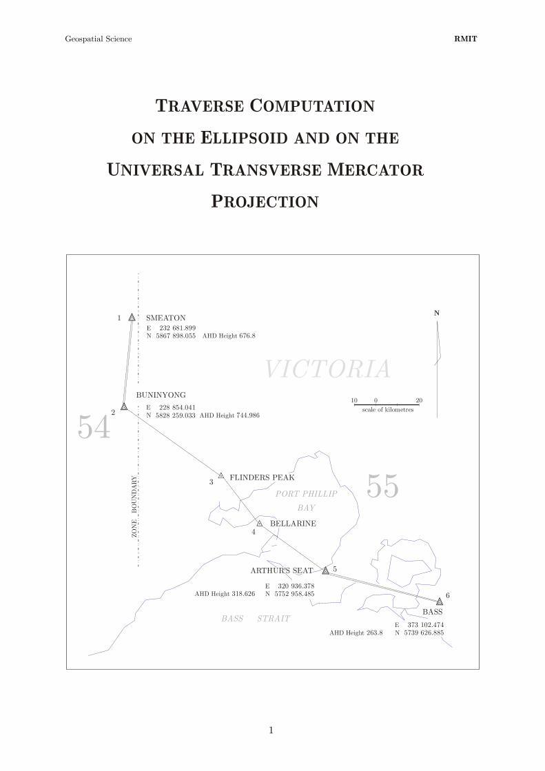
As an example of the reductions required a traverse between trigonometric stations
Buninyong, Flinders Peak, Bellarine and Arthur's Seat in Victoria is used. This traverse
should be well known to surveyors in Australia as it has been used to demonstrate reduction
techniques in The Australian Map Grid Technical Manual (NMC 1972), The Australian
Geodetic Datum Technical Manual (NMC 1985) and the Geocentric Datum of Australia
Technical Manual (ICSM 2002). In the latter publication the geodetic and grid coordinates
are Geocentric Datum of Australia 1994 (GDA94) and Map Grid Australia (MGA94) values
respectively. In the earlier publications the coordinates were Australian Geodetic Datum
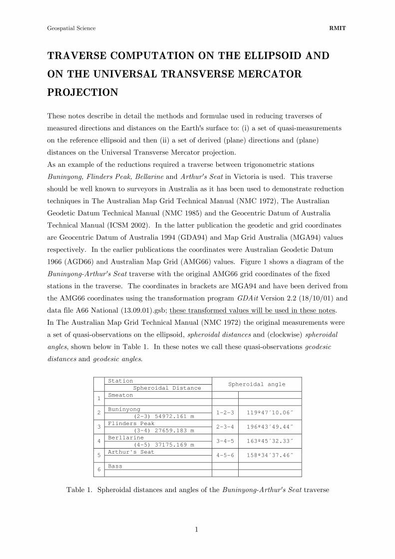
1966 (AGD66) and Australian Map Grid (AMG66) values. Figure 1 shows a diagram of the
Buninyong-Arthur's Seat traverse with the original AMG66 grid coordinates of the fixed
stations in the traverse. The coordinates in brackets are MGA94 and have been derived from
the AMG66 coordinates using the transformation program GDAit Version 2.2 (18/10/01) and
data file A66 National (13.09.01).gsb; these transformed values will be used in these notes.
In The Australian Map Grid Technical Manual (NMC 1972) the original measurements were
a set of quasi-observations on the ellipsoid, spheroidal distances and (clockwise) spheroidal
angles, shown below in Table 1. In these notes we call these quasi-observations geodesic
distances and geodesic angles.
Station Spheroidal Distance
Spheroidal angle
Smeaton 1 Buninyong 2 (2-3) 54972.161 m
1-2-3 119º47´10.06˝
Flinders Peak 3 (3-4) 27659.183 m
2-3-4 196º43´49.44˝
Berllarine 4 (4-5) 37175.169 m
3-4-5 163º45´32.33˝
Arthur's Seat 5
4-5-6 158º34´37.46˝
Bass 6
Table 1. Spheroidal distances and angles of the Buninyong-Arthur's Seat traverse
1
Geospatial Science RMIT
.
.
.
.
. SMEATON
BUNINYONG
FLINDERS PEAK
BELLARINE
ARTHUR'S SEAT
BASS
228 742.077
320 824.691
372 990.684
232 570.120 232 681.899
228 854.041
320 936.378
373 102.474
5828 074.208
5752 774.441
5739 442.811
5867 713.406 5867 898.055
5828 259.033
5752 958.485
5739 626.885
E
E
E
E E
E
E
E
N
N
N
N N
N
N
N
TRAVERSE DIAGRAM: BUNINYONG - ARTHUR'S SEATSHOWING FIXED DATA
Fixed Station
Floating Station
1
2
3
4
5
6
Coordinates shown below station names are
Australian Map Grid 1966, Zone 55
Coordinates shown in brackets are
Map Grid Australia 1994, Zone 55
N
10 0 20scale of kilometres
]
]
]
]NOTE: MGA94 coordinates derived from AMG66
coordinates using transformation program
Version 2.02 (18/10/01) and data file
A66 National (13.09.01).gsb
GDAit
ZO
NE B
OU
ND
ARY
54 55PORT PHILLIP
BAY
BASS STRAIT
VICTORIA
Figure 1. Buninyong-Arthur's Seat traverse
Data from: The Australian Map Grid Technical Manual, Special
Publication 7, National Mapping Council of Australia, 1972.
2

Geospatial Science RMIT
REDUCTION OF TRAVERSE MEASUREMENTS TO THE
ELLIPSOID
The traverse measurements to be considered are:
1. Horizontal directions measured with a theodolite,
2. Vertical circle observations measured with a theodolite,
3. Slope distances (or chord distances) derived from measurements made with
Electronic Distance Measuring (EDM) equipment.
Traverse measurements are made between points on the Earth's terrestrial surface and
traverse stations have complimentary points on the surface of the
reference ellipsoid; Q is the projection of P via the ellipsoid normal. The reduction of
measurements to the ellipsoid means applying a series of corrections to the measurements
made between points to obtain a set of quasi-measurements between points on the
ellipsoid. The corrections may be divided into gravimetric and geometric corrections;
gravimetric corrections applied first, followed by geometric corrections.
1 2, , , kP P P…
kP
1 2, , , kQ Q Q…
kQ
•
•
•
•
Q Q0
N
P0
P
normal
H
h
geoid
ellipsoid
vertical
ε
ε
t
s
er
r
le
astri
urface
equipote lntia
s
g
plumbline
Figure 2. Projection of P on the Earth's surface to Q on the ellipsoid and
on the geoid. Note that P, Q, and do not lie in the same
vertical plane since the plumbline is a 3D space curve.
0P
0P 0Q
Gravimetric corrections are applied to theodolite observations only. The rotational axis of a
theodolite (that is correctly levelled and in adjustment) is coincident with the vertical at P
and the horizontal plane of the theodolite is tangential to the equipotential surface of the
Earth's gravity field passing through P. In general, the vertical and the ellipsoid normal do
3

Geospatial Science RMIT
not coincide and gravimetric corrections are applied to the observations to create a set of
measurements with respect to the ellipsoid normal and geodetic horizon plane at P. The
geodetic horizon plane at P is a plane parallel to the plane tangential to the ellipsoid at Q.
Gravimetric corrections involve the deflection components (meridian plane) and η (prime
vertical plane) which must be obtained from a geoid model such as AUSGeoid98.
Gravimetric corrections are generally very small and are often ignored. In these notes they
will be computed and applied and the reader may gauge their applicability to other traverse
reductions.
ξ
Geometric corrections are applied to both theodolite and distance measurements.
SYMBOLS
THE GREEK ALPHABET
Alpha Iota Ι Rho Ρ Α α ι ρ
Beta Kappa Κ κ Sigma Σ Β β σ
Gamma Lambda Λ λ Tau Τ Γ γ τ
Delta Mu Μ Upsilon ϒ Δ δ μ υ
Epsilon Nu Ν Phi Ε ε ν Φ φ ϕ
Zeta Xi Ξ Chi Ζ ζ ξ Χ χ
Eta Omicron Ο ο Psi Η η Ψ ψ
Theta Pi Omega Ω Θ θ ϑ Π π ω
α = azimuth, clockwise from true north 0° to 360°
,A Gα α = astronomic azimuth and geodetic azimuth
12 21,α α = azimuth from point 1 to point 2 and azimuth from point 2 to point 1
β = grid bearing measured clockwise from Grid North, β α γ= +
γ = angle of refraction
γ = grid convergence, positive East of the central meridian and negative West
δ = arc-to-chord correction with sign defined by θ β δ= +
ε = deflection of the vertical in direction α and cos sinε ξ α η α= +
,s gε ε = deflections of the vertical at the Earth's surface and the geoid respectively
η = deflection of the vertical in the prime vertical plane
,s gη η = deflection of the vertical in the prime vertical plane at the earth's surface and
the geoid
θ = plane bearing measured clockwise from Grid North, θ β δ= +
ν = radius of curvature in prime vertical plane
1 2,ν ν = radius of curvature of ellipsoid in prime vertical plane at points 1 and 2
4

Geospatial Science RMIT
mν = ( )1 2 2ν ν+
ξ = deflection of the vertical in the meridian plane
,s gξ ξ = deflections of the vertical in the meridian plane at the Earth's surface and the
geoid
ρ = radius of curvature of ellipsoid in meridian plane
1 2,ρ ρ = radius of curvature of ellipsoid in meridian plane at points 1 and 2
mρ = ( )1 2 2ρ ρ+
φ = geodetic latitude, negative south of the equator
1 2,φ φ = latitude at points 1 and 2 respectively
mφ = ( )1 2 2φ φ+
s = geodesic distance (also ellipsoidal or spheroidal distance)
a, b = major and minor semi-axes of the ellipsoid 2e = square of the (first) eccentricity of the ellipsoid = ( )2 2a b a− 2
2e′ = square of the second eccentricity of the ellipsoid = ( )2 2a b b− 2
f = flattening of ellipsoid = ( )a b a−
h = ellipsoid height (height above ellipsoid measured along normal)
1 2,h h = ellipsoidal heights at points 1 and 2 respectively
H = orthometric height (height above geoid measured along plumbline)
K = Line Scale Factor
k = coefficient of refraction
k = Point Scale Factor
0k = central meridian scale factor = 0.9996
L = plane distance
N = h = geoid-ellipsoid separation H−
R = ρν = mean radius of curvature
Rα = radius of curvature of a normal section in a given azimuth 2
mr = for 20kρν ( )1 2 2mφ φ φ= +
z = zenith distance (vertical angle measured from the zenith)
5

Geospatial Science RMIT
REDUCTION FORMULA
The derivations of the following equations can be found in selected texts and references. No
attempt is made here to explain the derivations and the reader is directed to the references
for derivations and detailed discussion.
GRAVIMETRIC CORRECTIONS TO THEODOLITE
OBSERVATIONS
sin cos
corrected direction observed directiontan
s A s A
Az
ξ α η α⎧ ⎫⎪ ⎪− +⎪= +⎨⎪ ⎪⎪ ⎪⎩ ⎭
⎪⎬ (1)
corrected zenith distance observed zenith distance cos sins A s Aξ α η α= + + (2)
In equations (1) and (2) observed direction and zenith distance are measurements made at P
with a theodolite (that is correctly levelled and in adjustment) whose rotational axis is
coincident with the vertical at P and the horizontal plane of the theodolite is tangential to
the equipotential surface of the Earth's gravity field passing through P. Corrected direction
and zenith distance are quasi-measurements made at P with a theodolite whose rotational
axis is coincident with the normal at P and the horizontal plane of the theodolite is the
geodetic horizon plane at P (the geodetic horizon plane at P is a plane parallel to the plane
tangential to the ellipsoid at Q).
sξ and are deflections of the vertical (meridian and prime vertical respectively) and the
subscript s indicates that these are deflections at the terrestrial surface at P, see Figure 2
where . Deflections can be determined by observations, but are usually
computed from geoid models such as AUSGeoid98 in which case they are deflections of the
vertical at the geoid, denoted by and . The differences between , and , are
due to the gravimetric effects of the terrain between the geoid and the terrestrial surface in
the vicinity of P. They are difficult to model but they are usually very small (Featherstone
& Rüeger 2000). In these notes the differences are ignored and , is
assumed.
sη
cos sinε ξ α η α= +
gξ gη sξ
= =
sη
s gξ
gξ
η η= =
gη
ξ ξ s gη
Aα is azimuth and the subscript A indicates that it is astronomic azimuth, i.e., an angle with
respect to the observer's astronomic meridian (a meridian plane containing the north and
south poles and the vertical at P). is azimuth and the subscript G indicates that it is
geodetic azimuth, i.e., an angle with respect to the observer's geodetic meridian (a meridian
plane containing the north and south poles and the ellipsoid normal at P). The difference
Gα
6
Geospatial Science RMIT
between and is small and for the purposes of reduction equations Gα Aα
α α=
(1) and (2) it can be
assumed that . A Gα=
, ,G G hφ λ
REFERENCES
Featherstone, W.E. and Rüeger, J.M., 2000. 'The importance of using deflections of the
vertical for reduction of survey data to a geocentric datum', The Trans Tasman
Surveyor, Vol. 1, No. 3, pp. 46-61, December 2000. See also "Erratum" in The
Australian Surveyor, Vol. 47, No. 1, p.7, June 2002.
Heiskanen, W.A. and Moritz, H., 1967. Physical Geodesy, W.H. Freeman & Co., London,
pp. 184-88.
Vanicek, P. and Krakiwsky, E., 1986. Geodesy: The Concepts, North-Holland, Amsterdam.
RMIT Lecture Notes, Relationship Between Astronomic Coordinates and Geodetic
Coordinates , 8 pages.
, ,A A Hφ λ
GEOMETRIC CORRECTIONS TO THEODOLITE OBSERVATIONS
SKEW–NORMAL CORRECTION TO GEODETIC DIRECTIONS ON AN
ELLIPSOID
2 2212 2co n dir'n = observed normal section dir'n sin 2 cos
2 m
he α φ
ρ
⎧ ⎫⎪ ⎪⎪ ⎪+ ⎨ ⎬⎪ ⎪⎪ ⎪⎩ ⎭(3) rrect no sectiormal
where
is the ellipsoidal height of station 2 2h
( )2 2
( )( )
e f= f− is the (first) eccentricity squared and f is the ellipsoid flattening
2
2 21 si
a e−3 2
1
neρ
φ−= is the radius of curvature of the ellipsoid in the meridian plane
1 2
2m
ρ ρρ
+=
is the azimuth between points 1 and 2 12α
is the latitude of point 2 2φ
7
Geospatial Science RMIT
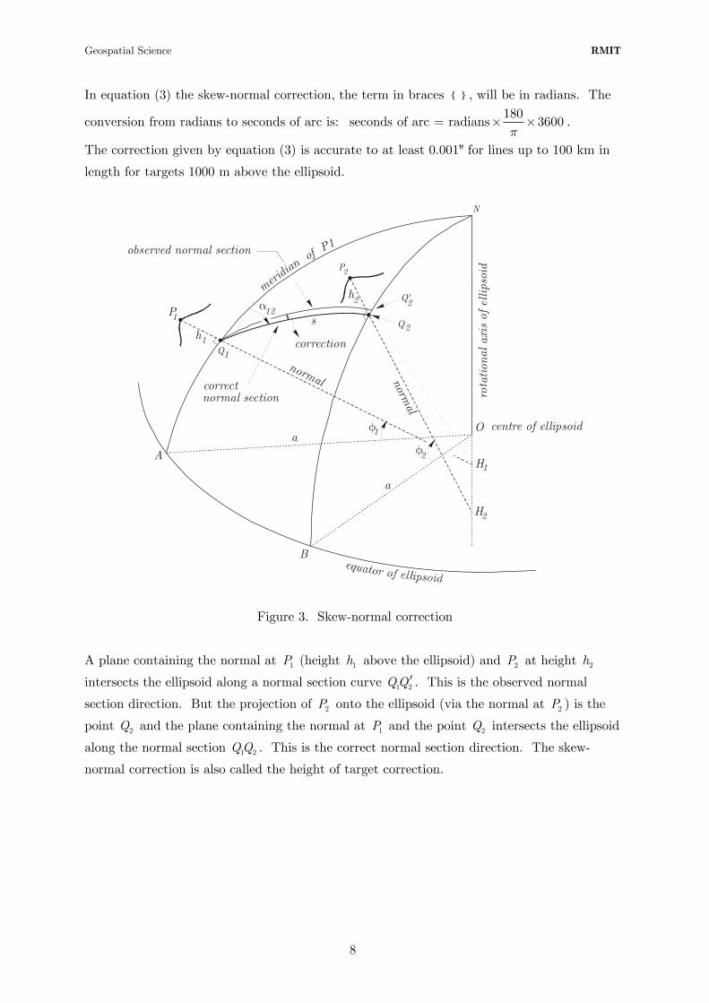
In equation (3) the skew-normal correction, the term in braces , will be in radians. The
conversion from radians to seconds of arc is: 180
seconds of arc = radians 3600π
× × .
The correction given by equation (3) is accurate to at least 0.001" for lines up to 100 km in
length for targets 1000 m above the ellipsoid.
P
P
1
2
h1Q1
h2
•
•
•
•
O
H1
H2
normal normal
meridia
n of
P1
Q'2
Q2
rot a
tion
al a
xis
of e
llips
oid
centre of ellipsoidφ1
φ2
α12s
N
A
B
a
a
correction
observed normal section
correct normal section
Figure 3. Skew-normal correction
A plane containing the normal at (height above the ellipsoid) and at height
intersects the ellipsoid along a normal section curve . This is the observed normal
section direction. But the projection of onto the ellipsoid (via the normal at ) is the
point and the plane containing the normal at and the point intersects the ellipsoid
along the normal section . This is the correct normal section direction. The skew-
normal correction is also called the height of target correction.
1P 1h 2P 2h
1 2QQ ′
2P 2P
2Q 1P 2Q
1 2QQ
8

Geospatial Science RMIT
CORRECTION FROM THE NORMAL SECTION DIRECTION TO THE
GEODESIC DIRECTION
2
2122geodesic direction = normal section direction sin 2 cos
12 mm
se α φ
ν
⎧ ⎫⎪ ⎪⎪+ −⎨⎪⎪ ⎪⎩ ⎭
2 ⎪⎬⎪ (4)
where
s is the geodesic distance on the ellipsoidal between points 1 and 2
( )2 2e f f= − is the (first) eccentricity squared and f is the ellipsoid flattening
( )1 22 21 sin
a
eν
φ=
− is the radius of curvature of the ellipsoid in the prime vertical
plane
1 2
2m
ν νν
+=
is the azimuth between points 1 and 2 12α
1
2m
φ φφ
+= 2 is the mean of latitudes of points 1 and 2
P
P
1
2
h1Q1
Q1
Q1
h2
•
•
•
•
O
H1
H2
normal normal
meridia
n of P
1
Q2
Q2
Q2ro
t ation
al a
xis
of e
llips
oid
centre of ellipsoidφ1
φ2
α12
α21
N
A
B
a
a
normal section
normal section
Figure 4. Reciprocal normal sections on the ellipsoid
9

Geospatial Science RMIT
A plane containing the ellipsoid normal at and the point (the projection of on the
ellipsoid) intersects the surface of the ellipsoid along the normal section curve QQ . The
reciprocal normal section curve (the intersection of the plane containing the normal at
and the point with the ellipsoidal surface) does not in general coincide with the
normal section curve although the distances along the two curves are for all practical
purposes the same. Hence there is not a unique normal section curve between and .
1P 2Q 2P
21
1Q
2 1Q Q
2P 1Q
1 2QQ
2Q
A geodesic is a unique curve on the
surface of an ellipsoid and is the line
of shortest distance between and
. In general, a geodesic lies
between the reciprocal normal
section curves and divides the angle
between the normal sections in the
ratio of 1/3 to 2/3.
1Q
2QQ
Q
1
2
geodesic
Q1Q2normal section
Q1Q2normal section
Δ
Δ⎯3
Figure 5. Geodesic curve between normal sections
In equation (4) the correction from the normal section to the geodesic, the term in braces
, will be in radians. The conversion from radians to seconds of arc is:
180
seconds of arc = radians 3600π
× × .
The correction given by equation (4) is accurate to at least 0.001" for lines up to 150 km in
length on the ellipsoid. At 1500 km, the correction is approximately 7" and the formula is
accurate to about 0.6". At greater distances the accuracy of the formula deteriorates and
other methods should be used to determine the correction.
The difference between the length of the geodesic and either of the normal sections seldom
attains 1 mm at 1500 km and can be ignored for all practical purposes (NMC 1985).
10

Geospatial Science RMIT
REFERENCES
Krakiwsky, E.J. and Thomson, D.B., 1974. Geodetic Position Computations, 1990 re-print,
Department of Surveying Engineering, University of Calgary, Calgary, Alberta,
Canada.
NMC, 1985. The Australian Geodetic Datum Technical Manual, Special Publication 10,
National Mapping Council of Australia, Canberra, 1985
RMIT Lecture Notes, Skew-normal Correction to Geodetic Directions on an Ellipsoid, 8
pages.
Vanicek, P. and Krakiwsky, E., 1986. Geodesy: The Concepts, North-Holland, Amsterdam.
DETERMINATION OF ELLIPSOIDAL HEIGHT DIFFERENCES
FROM VERTICAL CIRCLE THEODOLITE OBSERVATIONS AND
SLOPE DISTANCES
To reduce a chord distance (or slope distance) between points and on the Earth's
terrestrial surface to a distance s on the ellipsoid between the projections and , the
ellipsoidal heights and at and must be known. Ellipsoidal height differences
can be determined from vertical circle theodolite observations and measured
slope distances and ellipsoidal heights of successive points of a traverse determined from a
known starting height. Two formulae can be used; one using the chord distance D and the
other using the geodesic distance s
1P 2P
1Q 2Q
1h 2h 1P 2P
2h h hΔ = − 1
Chord distance (or slope distance) D known
( )2
212 2 1 1 1 1 2cos 1 2 sin
2D
h h h D z k z i gRα
Δ = − = + − + − (5)
Geodesic distance s known
( )2
112 2 1 1 2
1
1 1 2tan 2
h s sh h h k i g
R z Rα α
⎛ ⎞⎧ ⎫⎪ ⎪⎟⎪ ⎪⎜ ⎟Δ = − = + + − + −⎜ ⎨ ⎬⎟⎜ ⎟⎜ ⎟⎪ ⎪⎝ ⎠⎪ ⎪⎩ ⎭ (6)
where
D is the chord distance (or slope distance) between points 1 and 2
are the ellipsoidal heights of stations 1 and 2 1 2,h h
11
Geospatial Science RMIT
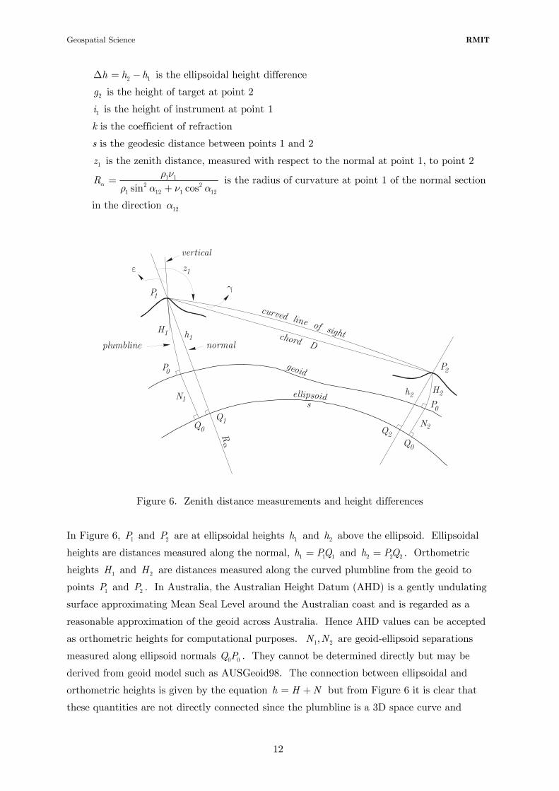
is the ellipsoidal height difference 2h h hΔ = − 1
is the height of target at point 2 2g
is the height of instrument at point 1 1i
k is the coefficient of refraction
s is the geodesic distance between points 1 and 2
is the zenith distance, measured with respect to the normal at point 1, to point 2 1z
1 12
1 12 1sin cosRα
ρ νρ α ν α
=+ 2
12
is the radius of curvature at point 1 of the normal section
in the direction 12α
geoid
ellipsoids
Rα
P1
P0
P0
P2
Q1Q0
Q0
Q2
plumbline
H2
H1
h2
h1
N2
N1
normal
curved line of sight
z1ε
vertical
chord D
γ
Figure 6. Zenith distance measurements and height differences
In Figure 6, and are at ellipsoidal heights and above the ellipsoid. Ellipsoidal
heights are distances measured along the normal, h and . Orthometric
heights and are distances measured along the curved plumbline from the geoid to
points and . In Australia, the Australian Height Datum (AHD) is a gently undulating
surface approximating Mean Seal Level around the Australian coast and is regarded as a
reasonable approximation of the geoid across Australia. Hence AHD values can be accepted
as orthometric heights for computational purposes. are geoid-ellipsoid separations
measured along ellipsoid normals . They cannot be determined directly but may be
derived from geoid model such as AUSGeoid98. The connection between ellipsoidal and
orthometric heights is given by the equation h H but from Figure 6 it is clear that
these quantities are not directly connected since the plumbline is a 3D space curve and
1P
P
2P 1h 2h
1PQ
1 N
N
1 =
2,N
= +
1 22 2h PQ=
1H
1P2H
2
0 0Q P
12
Geospatial Science RMIT
0, , and P Q P Q
cos sε ξ α η= +
0 are not collinear. Nevertheless, for all practical purposes h H can be
regarded as an exact relationship and AHD values can be substituted for H (Featherstone &
Rüeger 2000).
N= +
In equations (5) and (6), and Figure 6 is the zenith distance, measured with respect to the
normal at point 1, to the target at point 2, and theodolite vertical circle observations (made
with respect to the vertical) should first be corrected for gravimetric effects (the value
) before using in the formulae; see equation
1z
inα (2).
In Figure 6, the line of sight is curved or refracted by the Earth's atmosphere and γ is
a small angle, known as the angle of refraction, between the curved line of sight and the
chord D. By letting
1 2PP
k ks Rαγ θ= =
21hΔ
where k is the coefficient of refraction and θ is the
angle subtended by an arc length s at the centre of a circular arc of radius . The effects of
refraction are allowed for in the development of equations
Rα
(5) and (6) but the value of k
cannot be determined with any degree of certainty, since it is known to vary according to the
time of day, the atmospheric conditions, the length of line and the direction of the line of
sight. Using reciprocal verticals, i.e., vertical circle observations observed simultaneously
from both ends of the line, can eliminate this uncertainty assuming that the coefficient of
refraction will be the same (or nearly so) at both ends of the line. This assumption is valid if
the Earth's atmosphere is stable and evenly heated and from practice it is well known that
reciprocal verticals will only yield reliable height differences if the observing conditions are
reasonable and the observations are made between the hours of 11 am and 3 pm. When
using equations (5) or (6) a value of k = 0.07 for average conditions is used and height
differences and computed from observations at both ends; the mean result
assumed free of uncertainty in the value of k. For a complete treatment of the effects of
atmospheric refraction on vertical angles the reader is directed to Bomford (1980, pp. 228-
243)
12hΔ
It should be noted that some authors define the coefficient of refraction as a ratio of radii of
curvature, k Rα σ′ = where σ is the radius of curvature of the curved line of sight. This
leads to ( )2kγ θ′≈
1 2k−
or k . Equations 2k′ = (5) and (6) could contain the term ( rather
than ( ) .
)1 k ′−
Equations (5) and (6) are not exact relationships and certain practical assumptions are made
in their development (RMIT 1984). Similar equations are derived in Rüeger (1990, pp. 108-
114).
13
Geospatial Science RMIT
REFERENCES
Bomford, G., 1980. Geodesy, 4th edn, Clarendon Press, Oxford
Featherstone, W.E. and Rüeger, J.M., 2000. 'The importance of using deflections of the
vertical for reduction of survey data to a geocentric datum', The Trans Tasman
Surveyor, Vol. 1, No. 3, pp. 46-61, December 2000. See also "Erratum" in The
Australian Surveyor, Vol. 47, No. 1, p.7, June 2002.
Rüeger, J.M., 1990. Electronic Distance Measurement – An Introduction, 3rd edn, Springer-
Verlag, Berlin.
RMIT Lecture Notes, Heights by Vertical Angles, February 1984, 15 pages.
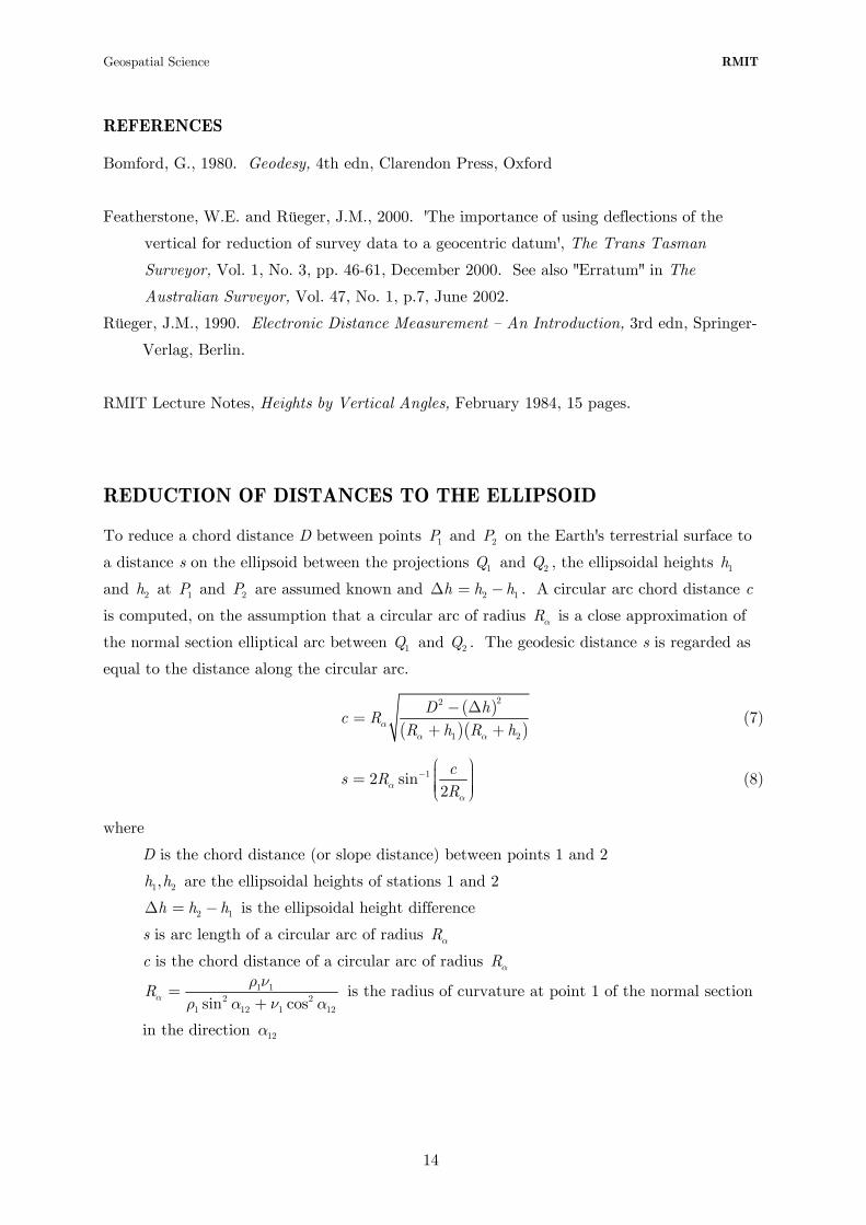
REDUCTION OF DISTANCES TO THE ELLIPSOID
To reduce a chord distance D between points and on the Earth's terrestrial surface to
a distance s on the ellipsoid between the projections and , the ellipsoidal heights
and at and are assumed known and . A circular arc chord distance c
is computed, on the assumption that a circular arc of radius is a close approximation of
the normal section elliptical arc between and . The geodesic distance s is regarded as
equal to the distance along the circular arc.
1P 2P
1Q
2 −2Q
1
Rα
1h
2h 1P 2P h h hΔ =
2Q1Q
( )
( )( )
22
1 2
D hc R
R h R hαα α
− Δ=
+ + (7)
12 sin2c
s RRα
α
−⎛ ⎞⎟⎜ ⎟= ⎜ ⎟⎜ ⎟⎜ ⎟⎝ ⎠
(8)
where
D is the chord distance (or slope distance) between points 1 and 2
are the ellipsoidal heights of stations 1 and 2 1 2,h h
is the ellipsoidal height difference 2h h hΔ = − 1
s is arc length of a circular arc of radius R α
c is the chord distance of a circular arc of radius R α
1 12
1 12 1sin cosRα
ρ νρ α ν α
=+ 2
12
is the radius of curvature at point 1 of the normal section
in the direction 12α
14

Geospatial Science RMIT
g ieo d
ellipsoids
Rα
P1
P2
Q1
Q2
h2
h1
chord D
chord c
O
normal
path length
Figure 7. The geometry of the reduction of measured slope distances
Figure 7 shows and at ellipsoidal heights and above the ellipsoid
and Δ = is the ellipsoidal height difference. The chord distance is the
measured slope distance. The actual distance measured by an EDM is the length of a curved
electromagnetic wave path called the raw-distance. Atmospheric corrections are applied and
a path curvature correction also applied to compensate for the difference between the mean
atmospheric conditions from observations at both ends of the line and the average
atmospheric conditions over the length of the line. The path length = raw-distance +
atmospheric correction + path curvature correction, is shown on Figure 7 as the curved path
. A correction is applied to the curved path length to give the chord distance D. It is
assumed, in these notes that all measured slope distances have been reduced to chord
distances D by the application of suitable corrections.
1P
1h−2P 1 1h PQ= 1 22 2h PQ=
2h h
2
1 2D PP=
1PP
In Figure 7, the normal section ellipsoidal arc between and is closely approximated by
a circular arc of radius with a centre at O and the ellipsoidal chord c can be assumed to
be a chord of a circular arc. The geodesic distance s is assumed, for all practical purposes, to
be equal to the arc length of a circular curve of radius R . This is a reasonable assumption
since for two points , , and , ,
on the GRS80 ellipsoid
1Q
α
2Q
2 =−
Rα
=−1 38φ 1 145λ = 1 1000 mh = 37φ 2 146λ =
1 1000 mh = ( ) the azimuth and 6378160,a f= = 1 298.2 22101572
15

Geospatial Science RMIT
geodesic distance are and . The geodesic distance
computed using equations
12 38 51 01.5705α ′ ′= ′ 141903.347 ms =
(7) and (8) is 141903.348 m, a difference of 0.001 m.
EXAMPLE TRAVERSE REDUCTIONS
Table 2 shows a set of observations made between the stations Smeaton, Buninyong, Flinders
Peak, Bellarine, Arthur's Seat and Bass and Figure 8 shows a diagram of the traverse.
Smeaton, Buninyong, Arthur's Seat and Bass are fixed stations and the coordinates of
Flinders Peak and Bellarine are required. No corrections have been applied to the theodolite
observations that are assumed to be the means of sets of horizontal directions (H) and
vertical circle observations (V). The slope distances are assumed to be chord distances
between observing stations.
Station Heights
AT TO Theodolite Observations
Slope distance Inst. Target
Buninyong Smeaton H 0º00´00˝ V 90º15´02.92˝ 1.650 1.650
Buninyong Flinders Peak H 119º47´10.10˝ V 90º37´42.36˝ 54978.184 1.650 1.585
Flinders Peak Buninyong H 0º00´00˝ V 89º47´52.25˝ 1.710 1.610
Flinders Peak Bellarine H 196º43´49.42˝ V 90º32´35.99˝ 27661.033 1.710 1.685
Bellarine Flinders Peak H 0º00´00˝ V 89º40´12.54˝ 1.660 1.760
Bellarine Arthur's Seat H 163º45´32.30˝ V 89º51´41.91˝ 37176.908 1.660 1.590
Arthur's Seat Bellarine H 0º00´00˝ V 90º25´24.13˝ 1.680 1.775
Arthur's Seat Bass H 158º34´37.43˝ V 90º15´57.84˝ 1.680 1.680
Table 2. Observations of the Buninyong-Arthur's Seat traverse
16

Geospatial Science RMIT
.
.
.
.
. SMEATON
BUNINYONG
FLINDERS PEAK
BELLARINE
ARTHUR'S SEAT
BASS
228 854.041
320 936.378
373 102.474
232 681.899
5828 259.033
5752 958.485
5739 626.885
5867 898.055
E
E
E
E
N
N
N
N
TRAVERSE DIAGRAM: BUNINYONG - ARTHUR'S SEATSHOWING FIXED DATA
Fixed Station
Floating Station
1
2
3
4
5
6
Coordinates are shown in terms of MGA94 Zone 55
N
10 0 20scale of kilometres
ZO
NE
BO
UN
DA
RY
54 55PORT PHILLIP
BAY
BASS STRAIT
VICTORIA
AHD Height 676.8
AHD Height 744.986
AHD Height 318.626
AHD Height 263.8
Figure 8. Buninyong-Arthur's Seat traverse
17

Geospatial Science RMIT
STEP 1 Computation of deflection of the vertical components ξ and η and geoid-ellipsoid
separations (N-values)
To apply gravimetric corrections to the theodolite observations, the deflection components
and need to be computed for each traverse station. This can be done using AUSGeoid98
available at the Geoscience Australia website (
ξ
η
http://www.ga.gov.au/) following the links
Geodesy & GPS, then AUSGeoid and finally Compute an N value on-line. The entry values required
are latitude and longitude and the computed output is an N-value (geoid-ellipsoid separation
in metres) and deflections ( ξ and in seconds of arc). η
The approximate latitudes and longitudes of the traverse stations can be computed using the
observed directions and slope distances and two Microsoft® Excel spreadsheets available at
the Geoscience Australia website by following the links to Geodetic Calculations then Calculate
Bearing Distance from Latitude Longitude. At this web page two Microsoft Excel spreadsheets are
available:
(i) Vincenty.xls will compute the direct case on the ellipsoid (given latitude and longitude of
point 1 and the azimuth and geodesic distance to point 2, compute latitude and
longitude of point 2) and the inverse case (given the latitudes and longitudes of points
1 and 2 compute the azimuth and geodesic distance between them) and
(ii) Redfearn.xls will convert GDA latitudes and longitudes on the ellipsoid to MGA East
and North coordinates on a Universal Transverse Mercator (UTM) projection with
point scale factor k and grid convergence and vice-versa. γ
1.1 Use Redfearn.xls to convert the Map Grid Australia (MGA94) Zone 55 grid coordinates
of the fixed stations Smeaton, Buninyong, Arthur's Seat and Bass to Geocentric Datum
of Australia (GDA94) latitudes and longitudes. The reference ellipsoid of GDA94 is the
reference ellipsoid of the Geodetic Reference System 1980 (GRS80)
6378137 m, 1 298.257222101a f= = . The computed latitudes and longitudes are
shown in Table 3. Station East North Latitude Longitude 1 Smeaton 232681.899 5867898.055 -37º17´49.7306˝ 143º59´03.1691˝ 2 Buninyong 228854.041 5828259.033 -37º39´10.1563˝ 143º55´35.3835˝ 5 Arthur's Seat 320936.378 5752958.485 -38º21´13.1263˝ 144º57´02.5549˝ 6 Bass 373102.474 5739626.885 -38º28´57.6104˝ 145º32´42.3666˝
Table 3. MGA Zone 55 and GDA coordinates of the fixed stations of the traverse.
18

Geospatial Science RMIT
1.2 Use Vincenty.xls to compute the geodesic azimuth and geodesic distance of the lines
Smeaton-Buninyong and Arthur's Seat-Bass. One will be the starting azimuth and the
other can be used as a check on the angular misclose of the traverse.
Line Station Azimuth α geodesic distance s 2-1 Buninyong-Smeaton 7º23´13.037˝ 39803.797 5-6 Arthur's Seat-Bass 105º36´33.043˝ 53848.539
Table 4. Geodesic azimuths and distances of fixed lines
1.3 Use the fixed azimuth of the line Buninyong-Smeaton (as the starting azimuth) and the
observed directions and slope distance (Table 2) to obtain approximations of the
geodesic azimuth and geodesic distance of the traverse line Buninyong-Flinders Peak.
Use these values ( ) and the GDA coordinates of
Buninyong in Vincenty.xls (Direct Solution) to compute the GDA coordinates of Flinders
Peak. The direct solution in Vincenty.xls will also give the reverse azimuth Flinders
Peak-Buninyong 3 , which is the starting azimuth for the next traverse
line Flinders Peak-Bellarine. This procedure is repeated for each traverse line and
Table 5 shows the computed results and the angular misclose of the traverse ( 0 ).
127 10 23.137 , 54978.184 msα ′ ′′≈ ≈
06 52 03.313′ ′′
.824′′ Observed traverse lines Azimuth Distance Point Buninyong (Fixed)
-37º39´10.1563˝ lat 143º55´35.3835˝ long
Buninyong-Smeaton (Fixed) Buninyong-Flinders Peak (obs)
7º23´13.037˝ + 119º47´10.10˝ = 127º10´23.137˝
54978.184
Flinders Peak (comp) -37º57´03.8222˝ 144º25´29.7304˝
Flinders Peak-Buninyong (comp) Flinders Peak-Bellarine (obs)
306º52´03.313˝ + 196º43´49.42˝ = 143º35´52.733˝
27661.033
Bellarine (comp) -38º09´05.3661˝ 144º36´43.9373˝
Bellarine-Flinders Peak (comp) Bellarine-Arthur's Seat (obs)
323º28´57.174˝ + 163º45´32.30˝ = 127º14´29.474˝
37176.908
Arthur's Seat (comp) -38º21´13.2868˝ 144º57´02.8792˝
Arthur's Seat-Bellarine (comp) Arthur's Seat-Bass (obs)
307º01´54.789˝ + 158º34´37.43˝ = 105º36´32.219˝
Arthur's Seat (Fixed) -38º21´13.1263˝ 144º57´02.5549˝
Arthur's Seat-Bass (Fixed) Misclose (Fixed-Observed)
105º36´33.043˝ - 105º36´32.219˝ = 0º00´00.824˝
Misclose (Fixed-comp) -0.1605˝ lat -0.3243˝ long
Table 5. Fixed and approximate GDA coordinates of traverse stations.
1.4 The geoid-ellipsoid separations (N-values) and deflection components and η are
computed using AUSGeoid98 available at the Geoscience Australia website
(
ξ
http://www.ga.gov.au/) following the links Geodesy & GPS, then AUSGeoid and finally
Compute an N value on-line. The entry values required are latitude and longitude (see
Table 5) and the computed values are shown in Table 6.
19

Geospatial Science RMIT
Station Latitude Longitude N ξ η 1 Smeaton -37º17´50˝ 143º59´03˝ 5.705 m +0.076˝ -6.554˝ 2 Buninyong -37º39´10˝ 143º55´35˝ 4.869 m -5.982˝ -3.817˝ 3 Flinders Peak -37º57´04˝ 144º25´30˝ 3.748 m -9.878˝ -1.606˝ 4 Bellarine -38º09´05˝ 144º36´44˝ 2.979 m -8.029˝ -2.453˝ 5 Arthur's Seat -38º21´13˝ 144º57´03˝ 3.095 m -2.557˝ -9.242˝ 6 Bass -38º28´58˝ 145º32´42˝ 3.904 m -5.169˝ -4.428˝
Table 6. Geoid-ellipsoid separations N and deflection components and . ξ η
The output from AUSGeoid98 rounds the latitudes and longitudes to the nearest second
of arc and ξ and η are components of the deflection of the vertical at the geoid.
STEP 2 Computation of gravimetric corrections to theodolite observations
Using equations (1) and (2), the azimuths of the traverse lines from Table 5, the deflection
components and from Table 6 and the theodolite observations from Table 2, corrections
to the theodolite observations are computed and shown in Table 7. The corrected theodolite
observations (H is horizontal direction and V is zenith distance) are quasi-measurements
made with a theodolite at P whose rotational axis is coincident with the normal at P and the
horizontal plane of the theodolite is the geodetic horizon plane at P (the geodetic horizon
plane at P is a plane parallel to the plane tangential to the ellipsoid at Q).
ξ η
Line Azimuth α Theodolite observations corr'ns
Theodolite observations
corrected to the normal
Buninyong- Smeaton 7º23´13.037˝ H 0º00´00˝
V 90º15´02.92˝ -0.020˝ -6.423˝
H 0º00´00˝ V 90º14´56.497˝
Buninyong- Flinders Peak 127º10´23.137˝ H 119º47´10.10˝
V 90º37´42.36˝ -0.027˝ +0.573˝
H 119º47´10.093˝ V 90º37´42.933˝
Flinders Peak- Buninyong 306º52´03.313˝ H 0º00´00˝
V 89º47´52.25˝ -0.024˝ -4.642˝
H 0º00´00˝ V 89º47´47.608˝
Flinders Peak- Bellarine 143º35´52.733˝ H 196º43´49.42˝
V 90º32´35.99˝ -0.043˝ +6.997˝
H 196º43´49.401˝ V 90º32´42.987˝
Bellarine- Flinders Peak 323º28´57.174˝ H 0º00´00˝
V 89º40´12.54˝ -0.016˝ -4.993˝
H 0º00´00˝ V 89º40´07.547˝
Bellarine- Arthur's Seat 127º14´29.474˝ H 163º45´32.30˝
V 89º51´41.91˝ +0.012˝ +2.906˝
H 163º45´32.328˝ V 89º51´44.816˝
Arthur's Seat- Bellarine 307º01´54.789˝ H 0º00´00˝
V 90º25´24.13˝ -0.026˝ +5.838˝
H 0º00´00˝ V 90º25´29.968˝
Arthur's Seat- Bass 105º36´33.043˝ H 158º34´37.43˝
V 90º15´57.84˝ +0.000˝ -8.213˝
H 158º34´37.456˝ V 90º15´49.627˝
Table 7. Theodolite observations, corrected to ellipsoid
normals, for the Buninyong-Arthur's Seat
traverse.
20
Geospatial Science RMIT
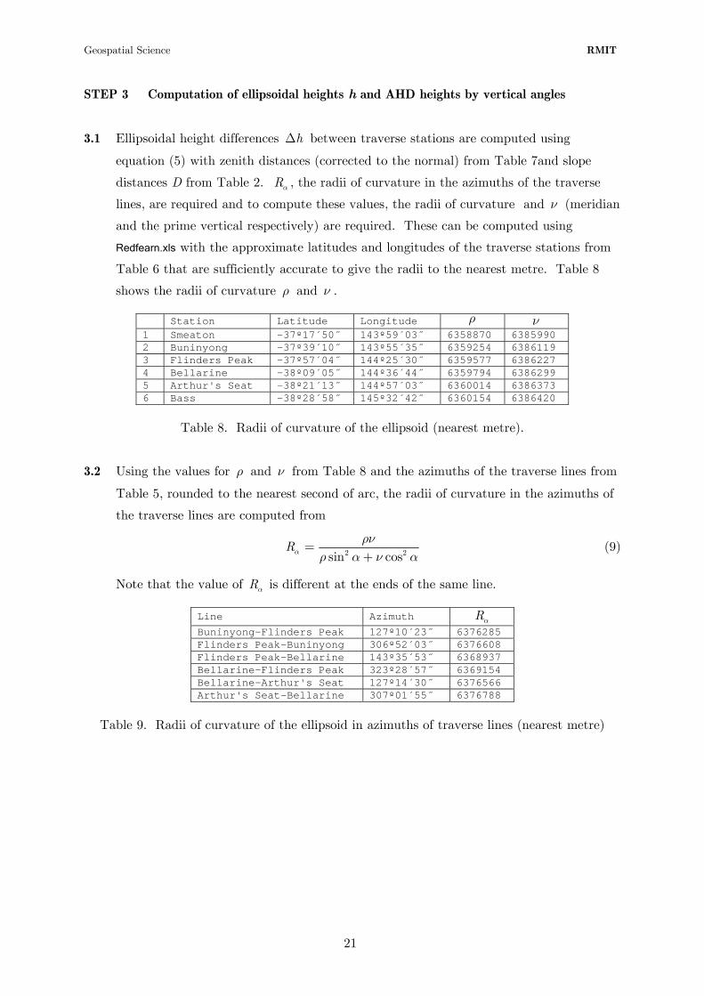
STEP 3 Computation of ellipsoidal heights h and AHD heights by vertical angles
3.1 Ellipsoidal height differences between traverse stations are computed using
equation
hΔ
α
ρ
(5) with zenith distances (corrected to the normal) from Table 7and slope
distances D from Table 2. R , the radii of curvature in the azimuths of the traverse
lines, are required and to compute these values, the radii of curvature and (meridian
and the prime vertical respectively) are required. These can be computed using
Redfearn.xls with the approximate latitudes and longitudes of the traverse stations from
Table 6 that are sufficiently accurate to give the radii to the nearest metre. Table 8
shows the radii of curvature and .
ν
ν
Station Latitude Longitude ρ ν 1 Smeaton -37º17´50˝ 143º59´03˝ 6358870 6385990 2 Buninyong -37º39´10˝ 143º55´35˝ 6359254 6386119 3 Flinders Peak -37º57´04˝ 144º25´30˝ 6359577 6386227 4 Bellarine -38º09´05˝ 144º36´44˝ 6359794 6386299 5 Arthur's Seat -38º21´13˝ 144º57´03˝ 6360014 6386373 6 Bass -38º28´58˝ 145º32´42˝ 6360154 6386420
Table 8. Radii of curvature of the ellipsoid (nearest metre).
3.2 Using the values for and from Table 8 and the azimuths of the traverse lines from
Table 5, rounded to the nearest second of arc, the radii of curvature in the azimuths of
the traverse lines are computed from
ρ ν
2sin cosRα
ρνρ α ν
=+ 2 α
(9)
Note that the value of is different at the ends of the same line. Rα
Line Azimuth Rα
Buninyong-Flinders Peak 127º10´23˝ 6376285 Flinders Peak-Buninyong 306º52´03˝ 6376608 Flinders Peak-Bellarine 143º35´53˝ 6368937 Bellarine-Flinders Peak 323º28´57˝ 6369154 Bellarine-Arthur's Seat 127º14´30˝ 6376566 Arthur's Seat-Bellarine 307º01´55˝ 6376788
Table 9. Radii of curvature of the ellipsoid in azimuths of traverse lines (nearest metre)
21

Geospatial Science RMIT
3.3 The ellipsoidal height differences , computed using equation hΔ (5) with as
the coefficient of refraction, are shown in Table 10 with mean results for each traverse
line.
0.07k =
Heights Line
Zenith
distance z
Slope distance
D Rα
Inst. Target
Height difference
hΔ
Buninyong- Flinders Peak 90º37´42.933˝ 54978.184 6376285 1.650 1.585 -399.277
Flinders Peak- Buninyong 89º47´47.608˝ 6376608 1.710 1.610 +399.136
Mean -399.207 Flinders Peak- Bellarine 90º32´42.987˝ 27661.033 6368937 1.710 1.685 -211.563
Bellarine- Flinders Peak 89º40´07.547˝ 6369154 1.660 1.760 +211.467
Mean -211.515 Bellarine- Arthur's Seat 89º51´44.816˝ 37176.908 6376566 1.660 1.590 +182.523
Arthur's Seat- Bellarine 90º25´29.968˝ 6376788 1.680 1.775 -182.658
Mean +182.590
Table 10. Computed ellipsoidal height differences and mean
height differences for the Buninyong-Arthur's Seat
traverse.
3.4 Ellipsoidal heights of the traverse stations are computed by adding the mean height
differences From Table 10 to the starting value at Buninyong:
744.986 4.869 749.855h H N= + = + =
Station Fixed
AHD Height H
N Ellipsoidal
Height h
Computed AHD Height
H 1 Smeaton 676.8 5.705 682.505 2 Buninyong 744.986 4.869 749.855
3 Flinders Peak 3.748
749.855 - 399.207 = 350.648 346.900
4 Bellarine 2.979
350.648 - 211.515 = 139.133 136.154
5 Arthur's Seat 318.626 3.095
139.133 + 182.590 = 321.723 318.628
6 Bass 263.8 3.904 267.704
Table 11. Ellipsoidal and AHD heights for the Buninyong-Arthur's Seat traverse.
Note that the height misclose, the difference between the Fixed and Computed AHD
Heights at Arthur's Seat, is not representative of height closures obtained from
verticals.
22
Geospatial Science RMIT
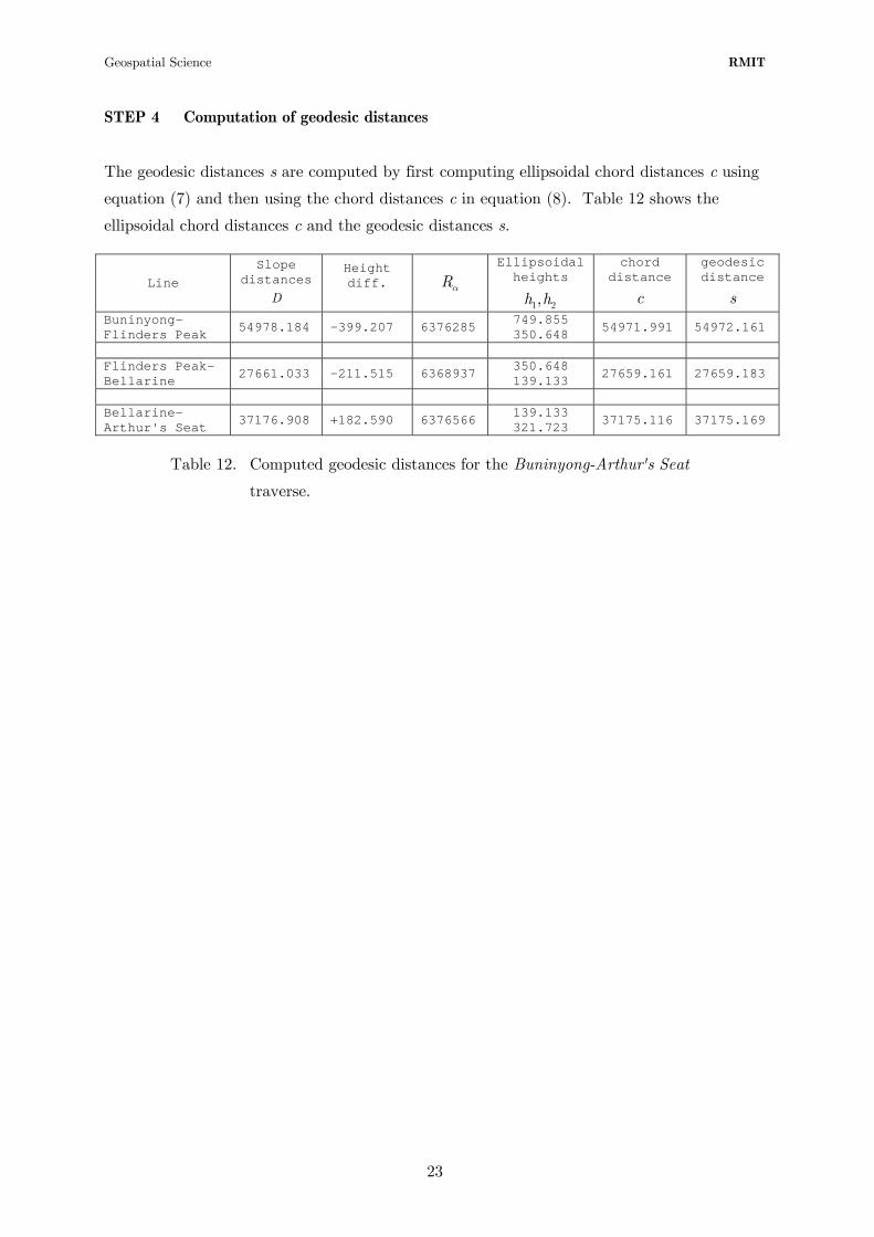
STEP 4 Computation of geodesic distances
The geodesic distances s are computed by first computing ellipsoidal chord distances c using
equation (7) and then using the chord distances c in equation (8). Table 12 shows the
ellipsoidal chord distances c and the geodesic distances s.
Line Slope
distances D
Height diff.
Rα
Ellipsoidal heights
1 2,h h
chord distance
c
geodesic distance
s Buninyong- Flinders Peak 54978.184 -399.207 6376285 749.855
350.648 54971.991 54972.161
Flinders Peak- Bellarine 27661.033 -211.515 6368937 350.648
139.133 27659.161 27659.183
Bellarine- Arthur's Seat 37176.908 +182.590 6376566 139.133
321.723 37175.116 37175.169
Table 12. Computed geodesic distances for the Buninyong-Arthur's Seat
traverse.
23
Geospatial Science RMIT
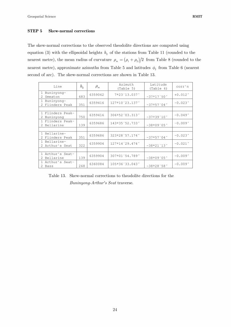
STEP 5 Skew-normal corrections
The skew-normal corrections to the observed theodolite directions are computed using
equation (3) with the ellipsoidal heights of the stations from Table 11 (rounded to the
nearest metre), the mean radius of curvature 2h
( )1 2 2mρ ρ ρ= + from Table 8 (rounded to the
nearest metre), approximate azimuths from Table 5 and latitudes from Table 6 (nearest
second of arc). The skew-normal corrections are shown in Table 13. 2φ
Line 2h mρ Azimuth (Table 5)
Latitude (Table 6) corr'n
1 Buninyong- 2 Smeaton 683 6359062 7º23´13.037˝ -37º17´50˝ +0.012˝
1 Buninyong- 2 Flinders Peak 351 6359416 127º10´23.137˝ -37º57´04˝ -0.023˝
1 Flinders Peak- 2 Buninyong 750 6359416 306º52´03.313˝ -37º39´10˝ -0.049˝
1 Flinders Peak- 2 Bellarine 139 6359686 143º35´52.733˝ -38º09´05˝ -0.009˝
1 Bellarine- 2 Flinders Peak 351 6359686 323º28´57.174˝ -37º57´04˝ -0.023˝
1 Bellarine- 2 Arthur's Seat 322 6359904 127º14´29.474˝ -38º21´13˝ -0.021˝
1 Arthur's Seat- 2 Bellarine 139 6359904 307º01´54.789˝ -38º09´05˝ -0.009˝
1 Arthur's Seat- 2 Bass 268 6360084 105º36´33.043˝ -38º28´58˝ -0.009˝
Table 13. Skew-normal corrections to theodolite directions for the
Buninyong-Arthur's Seat traverse.
24

Geospatial Science RMIT
STEP 6 Correction from the normal section to the geodesic
The corrections from the observed normal section directions to the geodesic directions are
computed using equation (4) with the geodesic distances s from Tables 4 and 12, the mean
radius of curvature ( )1 2 2mν ν ν= + from Table 8 (rounded to the nearest metre),
approximate azimuths from Table 5 and mean latitudes ( )1 2 2mφ φ φ= + from Table 6
(nearest second of arc). The corrections from the observed normal section directions to the
geodesic directions are shown in Table 14.
Line s mν Azimuth 12
(Table 5) α Latitude
mφ(Table 6)
corr'n
1 Buninyong- 2 Smeaton 38903.797 6386055 7º23´13.037˝ -37º28´30˝ -0.001˝
1 Buninyong- 2 Flinders Peak 54972.161 6386173 127º10´23.137˝ -37º48´07˝ +0.005˝
1 Flinders Peak- 2 Buninyong 54972.161 6386173 306º52´03.313˝ -37º48´07˝ +0.005˝
1 Flinders Peak- 2 Bellarine 27659.183 6386263 143º35´52.733˝ -38º03´05˝ +0.001˝
1 Bellarine- 2 Flinders Peak 27659.183 6386263 323º28´57.174˝ -38º03´05˝ +0.001˝
1 Bellarine- 2 Arthur's Seat 37175.169 6386336 127º14´29.474˝ -38º15´09˝ +0.002˝
1 Arthur's Seat- 2 Bellarine 37175.169 6386336 307º01´54.789˝ -38º15´09˝ +0.002˝
1 Arthur's Seat- 2 Bass 53849.539 6386396 105º36´33.043˝ -38º25´06˝ +0.003˝
Table 14. Corrections from normal section directions to geodesic directions.
25

Geospatial Science RMIT
STEP 7 Calculation of geodesic directions
The directions of the geodesics on the ellipsoid (geodesic directions) are obtained by adding
the skew-normal corrections (Table 13) and the corrections from the normal section to the
geodesic (Table 14) to the theodolite directions corrected to the normal (Table 7). Table 15
shows the geodesic directions reduced to 0 0 on the backsight. 0 00′ ′′
corrections Line
Theodolite directions corrected to the normal
skew-normal geodesic
Geodesic directions
Buninyong- Smeaton 0º00´00˝ +0.012˝ -0.001˝ 0º00´00˝
Buninyong- Flinders Peak 119º47´10.093˝ -0.023˝ +0.005˝ 119º47´10.064˝
Flinders Peak- Buninyong 0º00´00˝ -0.049˝ +0.005˝ 0º00´00˝
Flinders Peak- Bellarine 196º43´49.401˝ -0.009˝ +0.001˝ 196º43´49.437˝
Bellarine- Flinders Peak 0º00´00˝ -0.023˝ +0.001˝ 0º00´00˝
Bellarine- Arthur's Seat 163º45´32.328˝ -0.021˝ +0.002˝ 163º45´32.331˝
Arthur's Seat- Bellarine 0º00´00˝ -0.009˝ +0.002˝ 0º00´00˝
Arthur's Seat- Bass 158º34´37.456˝ -0.009˝ +0.003˝ 158º34´37.457˝
Table 15. Geodesic directions, for the Buninyong-Arthur's Seat
traverse.
STEP 8 Traverse observations reduced to the ellipsoid
Table 16 shows the set of measurements on the ellipsoid that are used to compute the Map
Grid Australia (MGA94) coordinates of the traverse stations Flinders Peak and Bellarine.
Station Geodesic Distance
Geodesic angle
Smeaton 1 Buninyong 2 (2-3) 54972.161 m
1-2-3 119º47´10.06˝
Flinders Peak 3 (3-4) 27659.183 m
2-3-4 196º43´49.44˝
Berllarine 4 (4-5) 37175.169 m
3-4-5 163º45´32.33˝
Arthur's Seat 5
4-5-6 158º34´37.46˝
Bass 6
Table 16. Geodesic distances and angles of the Buninyong-Arthur's Seat traverse
26

Geospatial Science RMIT
COMMENTARY ON THE REDUCTION OF OBSERVATIONS TO
THE ELLIPSOID
The reduction of traverse observations to the ellipsoid set out on the previous pages may be
regarded as exact for all practical purposes for traverse lines up to 55 km in length. For
shorter traverse lines certain corrections may be ignored without any practical loss of
accuracy, e.g., inspection of Tables 7 and 15 show that corrections to observed horizontal
directions (gravimetric, skew-normal and geodesic) do not exceed 0.03" for the Buninyong-
Arthur's Seat traverse. It would be a safe to ignore these corrections for traverse lines less
than 10 km in length and assume that observed traverse directions are, for practical
purposes, directions of geodesics on the ellipsoid.
Gravimetric corrections to vertical circle observations are often ignored in practice. This is
justified for the following reasons:
(i) The vertical circle observations are only used to determine ellipsoidal heights for
distance reduction, if gravimetric corrections to directions are ignored, and the equation
used for computing height differences contains an unknown quantity k, the coefficient of
refraction.
(ii) To allow for the error in k by assuming a representative value, say , only a
mean height difference from reciprocal vertical circle observations is regarded as correct.
0.07k =
(iii) If the geoid slope with respect to the ellipsoid is fairly constant along a particular
traverse line then the corrections for the deflection of the vertical will be of opposite
sign but approximately equal in magnitude and their effects will cancel in the
calculation of the mean height difference.
27

Geospatial Science RMIT
COMPUTATION OF MAP GRID AUSTRALIA (MGA94)
COORDINATES
Map Grid Australia (MGA94) coordinates are coordinates related to a grid superimposed
over a Universal Transverse Mercator (UTM) projection of latitudes and longitudes related
to the Geocentric Datum of Australia (GDA94). The 94 in MGA94 and GDA94 refer to the
date of the particular realization of the GDA coordinate set (latitudes and longitudes). The
GDA is defined by the size and shape of the reference ellipsoid, the ellipsoid of the Geodetic
Reference System 1980 (GRS80) – semi-major axis a = 6378137 m, flattening f =
1/298.257222101 – and the coordinates of the eight reference stations in the Australian
Fiducial Network (AFN). The coordinates of the AFN stations were derived from a global
adjustment of geodetic observations and are related to the International Terrestrial Reference
Frame of 1992 (ITRF92) at the epoch 1994.0; this effectively fixes the reference ellipsoid at
the centre of mass of the Earth with an axis coincident with the Earth's rotational axis as at
1994. The national geodetic data set, consisting of distances, directions and GPS
observations between stations in the Australian national geodetic network, was adjusted to
fit with the AFN yielding the GDA94 coordinate set.
The UTM projection is a Transverse Mercator (TM) projection of the ellipsoid with defined
zone widths and numbering, a central meridian scale factor and a true origin of
coordinates in a zone at the intersection of the equator and the central meridian. MGA94
coordinates are related to a false origin 10,000,000 m south and 500,000 m west of the true
origin of a UTM zone.
0 0.9996k =
GDA94 latitudes and longitudes and MGA94 East and North coordinates are related by
Redfearn's formulae, published by J.C.B Redfearn of the Hydrographic Department of the
British Admiralty in the Empire Survey Review (now Survey Review) in 1948 (Redfearn
1948). Redfearn noted in his five-page paper that: "…formulae of the projection itself have
been given by various writers, from Gauss, Schreiber and Jordan to Hristow, Tardi, Lee,
Hotine and others – not, it is to be regretted, with complete agreement in all cases."
Redfearn's formulae, accurate anywhere within zones of 10°–12° extent in longitude, removed
this "disagreement" between previous published formulae and are regarded as the definitive
TM formulae. Redfearn provided no method of derivation but mentioned techniques
demonstrated by Lee and Hotine in previous issues of the Empire Survey Review. In 1952,
the American mathematician Paul D. Thomas published a detailed derivation of the TM
formulae in Conformal Projections in Geodesy and Cartography, Special Publication No. 251
28
Geospatial Science RMIT
of the Coast and Geodetic Survey, U.S. Department of Commerce (Thomas 1952); Thomas'
work can be regarded as the definitive derivation of the TM formulae.
The conversion between GDA94 and MGA94 coordinates and the computation of azimuths
and geodesic distances on the ellipsoid can be achieved using the Microsoft Excel
spreadsheets Redfearn.xls and Vincenty.xls available on the Geoscience Australia website
(http://www.ga.gov.au) by following the links to Geodetic Calculations then Calculate Bearing
Distance from Latitude Longitude. At this web page two Microsoft Excel spreadsheets are
available:
(i) Vincenty.xls will compute the direct case on the ellipsoid (given latitude and longitude of
point 1 and the azimuth and geodesic distance to point 2, compute latitude and
longitude of point 2) and the inverse case (given the latitudes and longitudes of points
1 and 2 compute the azimuth and geodesic distance between them) and
(ii) Redfearn.xls will convert GDA94 latitudes and longitudes on the ellipsoid to MGA94
East and North coordinates on a Universal Transverse Mercator (UTM) projection with
point scale factor k and grid convergence and vice-versa. γ
These two spreadsheets make the computation of traverses a relatively simple matter.
There are two methods of computing the MGA94 coordinates of Flinders Peak and Bellarine
in the Buninyong-Arthur's Seat traverse. The first method, Traverse Computation on the
Ellipsoid is a simple direct method, but until recently, has not been practical due to the lack
of computational resources. This is no longer the case as any reasonable computer capable of
running the Excel spreadsheets Redfearn.xls and Vincenty.xls is adequate (ICSM 2002). The
second method, Traverse Computation on the UTM Map Plane (NMC 1972, NMC 1985) is a
more time consuming indirect method involving iteration. The second method of traverse
computation has been, up until now, the only method available to the general practitioner
lacking adequate computer resources. Featherstone and Kirby (2002) give an outline of the
two methods demonstrating that they give numerically equivalent results (1-3 mm agreement
in grid coordinates) and that the second method of computing MGA94 traverse coordinates
takes about three times longer than the first method.
29
Geospatial Science RMIT
TRAVERSE COMPUTATION ON THE ELLIPSOID
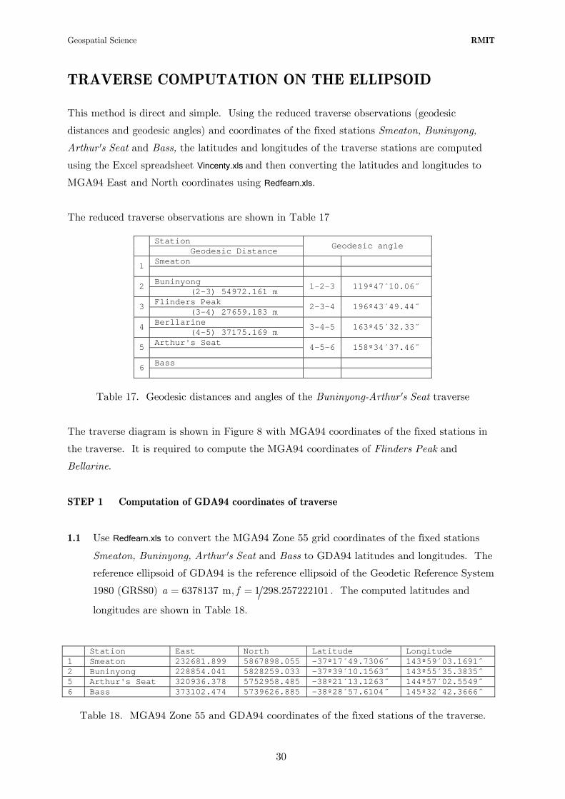
This method is direct and simple. Using the reduced traverse observations (geodesic
distances and geodesic angles) and coordinates of the fixed stations Smeaton, Buninyong,
Arthur's Seat and Bass, the latitudes and longitudes of the traverse stations are computed
using the Excel spreadsheet Vincenty.xls and then converting the latitudes and longitudes to
MGA94 East and North coordinates using Redfearn.xls.
The reduced traverse observations are shown in Table 17
Station Geodesic Distance
Geodesic angle
Smeaton 1 Buninyong 2 (2-3) 54972.161 m
1-2-3 119º47´10.06˝
Flinders Peak 3 (3-4) 27659.183 m
2-3-4 196º43´49.44˝
Berllarine 4 (4-5) 37175.169 m
3-4-5 163º45´32.33˝
Arthur's Seat 5
4-5-6 158º34´37.46˝
Bass 6
Table 17. Geodesic distances and angles of the Buninyong-Arthur's Seat traverse
The traverse diagram is shown in Figure 8 with MGA94 coordinates of the fixed stations in
the traverse. It is required to compute the MGA94 coordinates of Flinders Peak and
Bellarine.
STEP 1 Computation of GDA94 coordinates of traverse
1.1 Use Redfearn.xls to convert the MGA94 Zone 55 grid coordinates of the fixed stations
Smeaton, Buninyong, Arthur's Seat and Bass to GDA94 latitudes and longitudes. The
reference ellipsoid of GDA94 is the reference ellipsoid of the Geodetic Reference System
1980 (GRS80) 6378137 m, 1 298.257222101a f= = . The computed latitudes and
longitudes are shown in Table 18.
Station East North Latitude Longitude 1 Smeaton 232681.899 5867898.055 -37º17´49.7306˝ 143º59´03.1691˝ 2 Buninyong 228854.041 5828259.033 -37º39´10.1563˝ 143º55´35.3835˝ 5 Arthur's Seat 320936.378 5752958.485 -38º21´13.1263˝ 144º57´02.5549˝ 6 Bass 373102.474 5739626.885 -38º28´57.6104˝ 145º32´42.3666˝
Table 18. MGA94 Zone 55 and GDA94 coordinates of the fixed stations of the traverse.
30

Geospatial Science RMIT
1.2 Use Vincenty.xls to compute the geodesic azimuth and geodesic distance of the lines
Smeaton-Buninyong and Arthur's Seat-Bass. One will be the starting azimuth and the
other can be used as a check on the angular misclose of the traverse.
Line Station Azimuth α geodesic distance s 2-1 Buninyong-Smeaton 7º23´13.037˝ 39803.797 5-6 Arthur's Seat-Bass 105º36´33.043˝ 53848.539
Table 19. Geodesic azimuths and distances of fixed lines
1.3 Use the fixed azimuth of the line Buninyong-Smeaton (as the starting azimuth) and the
reduced geodesic distances and angles (Table 17) to obtain the geodesic azimuth and
geodesic distance of the traverse line Buninyong-Flinders Peak. Use these values
( and ) and the GDA94 coordinates of Buninyong
in Vincenty.xls (Direct Solution) to compute the GDA94 coordinates of Flinders Peak. The
direct solution in Vincenty.xls will also give the reverse azimuth Flinders Peak-Buninyong
, which is the starting azimuth for the next traverse line Flinders Peak-
Bellarine. This procedure is repeated for each traverse line and Table 20 shows the
computed results and the angular misclose of the traverse ( 0 ).
127 10 23.097α ′ ′=
306 52 03.394′ ′′
′ 54972.161 ms =
.598′′ Observed traverse lines Azimuth Distance Point Buninyong (Fixed)
-37º39´10.1563˝ lat 143º55´35.3835˝ long
Buninyong-Smeaton (Fixed) Buninyong-Flinders Peak (obs)
7º23´13.037˝ + 119º47´10.06˝ = 127º10´23.097˝
54972.161
Flinders Peak (comp) -37º57´03.7047˝ 144º25´29.5333˝
Flinders Peak-Buninyong (comp) Flinders Peak-Bellarine (obs)
306º52´03.394˝ + 196º43´49.44˝ = 143º35´52.834˝
27659.183
Bellarine (comp) -38º09´05.2006˝ 144º36´43.6943˝
Bellarine-Flinders Peak (comp) Bellarine-Arthur's Seat (obs)
323º28´57.303˝ + 163º45´32.33˝ = 127º14´29.633˝
37175.169
Arthur's Seat (comp) -38º21´13.0881˝ 144º57´02.5776˝
Arthur's Seat-Bellarine (comp) Arthur's Seat-Bass (obs)
307º01´54.985˝ + 158º34´37.46˝ = 105º36´32.445˝
Arthur's Seat (Fixed) -38º21´13.1263˝ 144º57´02.5549˝
Arthur's Seat-Bass (Fixed) Misclose (Fixed-Observed)
105º36´33.043˝ - 105º36´32.445˝ = 0º00´00.598˝
Misclose (Fixed-comp) +0.0382˝ lat -0.0227˝ long
Table 20. Fixed and computed GDA coordinates of traverse stations.
31
Geospatial Science RMIT
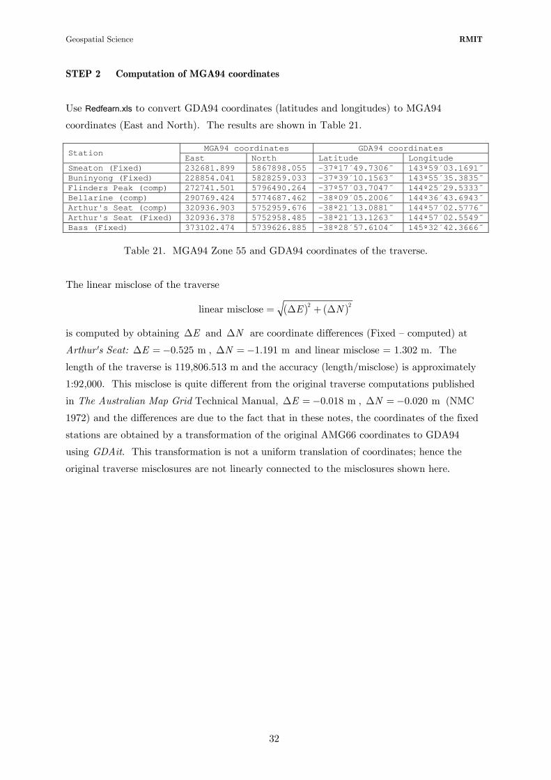
STEP 2 Computation of MGA94 coordinates
Use Redfearn.xls to convert GDA94 coordinates (latitudes and longitudes) to MGA94
coordinates (East and North). The results are shown in Table 21.
MGA94 coordinates GDA94 coordinates Station East North Latitude Longitude
Smeaton (Fixed) 232681.899 5867898.055 -37º17´49.7306˝ 143º59´03.1691˝Buninyong (Fixed) 228854.041 5828259.033 -37º39´10.1563˝ 143º55´35.3835˝Flinders Peak (comp) 272741.501 5796490.264 -37º57´03.7047˝ 144º25´29.5333˝Bellarine (comp) 290769.424 5774687.462 -38º09´05.2006˝ 144º36´43.6943˝Arthur's Seat (comp) 320936.903 5752959.676 -38º21´13.0881˝ 144º57´02.5776˝Arthur's Seat (Fixed) 320936.378 5752958.485 -38º21´13.1263˝ 144º57´02.5549˝Bass (Fixed) 373102.474 5739626.885 -38º28´57.6104˝ 145º32´42.3666˝
Table 21. MGA94 Zone 55 and GDA94 coordinates of the traverse.
The linear misclose of the traverse
( ) ( )2 2linear misclose E N= Δ + Δ
is computed by obtaining and are coordinate differences (Fixed – computed) at
Arthur's Seat:
EΔ
525
NΔ
0. mEΔ =− , 1.191 m−NΔ = and linear misclose = 1.302 m. The
length of the traverse is 119,806.513 m and the accuracy (length/misclose) is approximately
1:92,000. This misclose is quite different from the original traverse computations published
in The Australian Map Grid Technical Manual, 0.018 mΔ =−E , 0.020 mNΔ =− (NMC
1972) and the differences are due to the fact that in these notes, the coordinates of the fixed
stations are obtained by a transformation of the original AMG66 coordinates to GDA94
using GDAit. This transformation is not a uniform translation of coordinates; hence the
original traverse misclosures are not linearly connected to the misclosures shown here.
32

Geospatial Science RMIT
TRAVERSE COMPUTATION ON THE UNIVERSAL
TRANSVERSE MERCATOR (UTM) PROJECTION
The Transverse Mercator (TM) projection is a conformal projection, i.e., the scale factor at a
point is the same in every direction, which means that shape is preserved, although this
useful property only applies to differentially small regions of the Earth's surface. Meridians
and parallels of the ellipsoid are projected as an orthogonal network of curves, excepting the
equator and a central meridian, which are projected as straight lines intersecting at right
angles. The intersection of the equator and the central meridian is known as the true origin
of coordinates and the scale factor along the central meridian is constant.
X
Y
λ0
equator
cent
ral
mer
idia
n
Figure 9. Transverse Mercator projection of part of the ellipsoid.
Central meridian , graticule interval 15º 0 105λ =
The TM projection is very useful for mapping regions of the Earth with large extents of
latitude, but for areas away from the central meridian, distortions increase rapidly. To limit
the effects of distortion, TM projections are usually restricted to small zones of longitude
about a central meridian . The Universal Transverse Mercator (UTM) projection is a TM
projection of the ellipsoid with defined zone widths of 6º of longitude (3º either side of the
central meridian), a zone numbering system (60 zones of 6º width, with zone 1 having a
central meridian 177º W and zone 60 having a central meridian of 177º E), a central
0λ
33

Geospatial Science RMIT
meridian scale factor and a true origin of coordinates for each zone at the
intersection of the equator and the central meridian. To make coordinates positive
quantities, each zone has an origin of East and North coordinates (known as the false origin)
located 500,000 m west along the equator from the true origin for the northern hemisphere,
and 500,000 m west and 10,000,000 m south of the true origin for the southern hemisphere.
0 0.9996k =
Figure 10 shows a schematic
diagram of a UTM zone of the
Earth. In the southern
hemisphere the point P will
have negative coordinates E',N'
related to the true origin at the
intersection of the central
meridian and the equator. P
has positive E,N coordinates
related to the false origin
500,000 m west and
10,000,000 m south of the true
origin. True origin and false
origin coordinates in the
southern hemisphere are related
by
equator
cent
ral
mer
idia
n
N'
E'
N
E
N
E
·
·
·
·
·
True Origin
False Origin offsetwest
offsetsouth
False originP
λ0
500, 000
10, 000, 000
E E
N N
′ = −
′ = − (10)
Figure 10 Schematic diagram of a UTM zone
showing false origins for the
northern and southern hemispheres
34
Geospatial Science RMIT
λ
φ
cent
ral
m
erid
ian
GNTN
γ
sL
θβ
projected geodesic
planedistance
1λ2
1
φ2
P2
P1
N
N
2
1
E
E
2
1
δ12
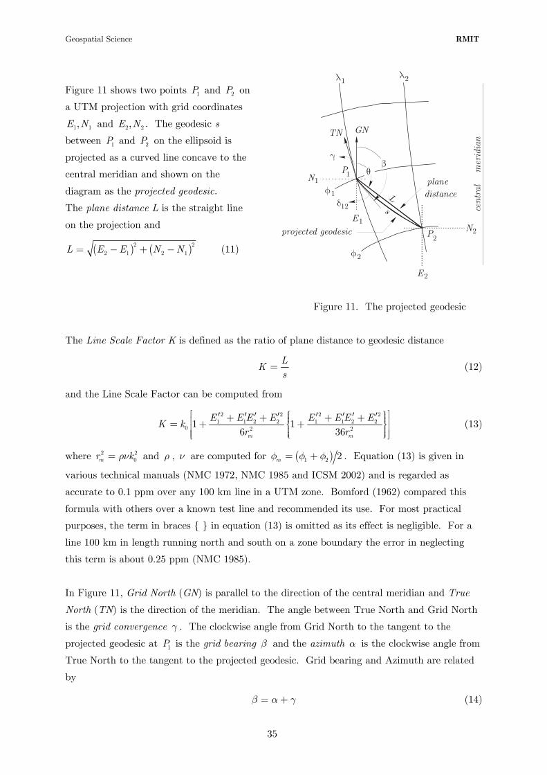
Figure 11 shows two points and on
a UTM projection with grid coordinates
and . The geodesic s
between and on the ellipsoid is
projected as a curved line concave to the
central meridian and shown on the
diagram as the projected geodesic.
1P 2P
1 1,E N 2,E N
2P2
)
1P
The plane distance L is the straight line
on the projection and
( ) (2
2 1 2 1L E E N N= − + − 2 (11)
Figure 11. The projected geodesic
The Line Scale Factor K is defined as the ratio of plane distance to geodesic distance
L
Ks
= (12)
and the Line Scale Factor can be computed from
2 2 2 2
1 1 2 2 1 1 2 20 21 1
6 36m m
E E E E E E E EK k
r r
⎡ ⎤⎧ ⎫′ ′ ′ ′ ′ ′ ′ ′⎪ ⎪+ + + +⎪⎢ ⎥= + +⎨⎢ ⎥⎪⎢ ⎥⎪ ⎪⎩ ⎭⎣ ⎦2
⎪⎬⎪
k )
(13)
where r and , are computed for 2 20m ρν= ρ ν ( 1 2 2mφ φ . Equation φ= + (13) is given in
various technical manuals (NMC 1972, NMC 1985 and ICSM 2002) and is regarded as
accurate to 0.1 ppm over any 100 km line in a UTM zone. Bomford (1962) compared this
formula with others over a known test line and recommended its use. For most practical
purposes, the term in braces in equation (13) is omitted as its effect is negligible. For a
line 100 km in length running north and south on a zone boundary the error in neglecting
this term is about 0.25 ppm (NMC 1985).
In Figure 11, Grid North (GN) is parallel to the direction of the central meridian and True
North (TN) is the direction of the meridian. The angle between True North and Grid North
is the grid convergence . The clockwise angle from Grid North to the tangent to the
projected geodesic at P is the grid bearing and the azimuth α is the clockwise angle from
True North to the tangent to the projected geodesic. Grid bearing and Azimuth are related
by
γ
1 β
(14) β α γ= +
35
Geospatial Science RMIT
By convention, in Australia, the grid convergence is a negative quantity west of the central
meridian and a positive quantity east of the central meridian.
In Figure 11, the plane bearing is the clockwise angle from Grid North to the straight line
joining and . The plane bearing is computed from plane trigonometry as
θ
1P 2P
1 2 1
2 1
tanE EN N
θ −⎛ ⎞− ⎟⎜ ⎟= ⎜ ⎟⎜ ⎟⎜ ⎟−⎝ ⎠
(15)
The small angle between the tangent to the projected geodesic at and the straight line
joining and is the arc-to-chord correction and is given by 1P
1P 2P 12δ
( )( ) ( )22 1 2 1 2 1
12 2
2 21
6 2m m
N N E E E E
r rδ
⎧ ⎫⎪ ⎪′ ′ ′ ′− + +⎪⎪= − −⎨⎪ ⎪⎪ ⎪⎪ ⎪⎩ ⎭27
⎪⎪⎬
k )
(16)
where and , are computed for 2 20mr ρν= ρ ν ( 1 2 2mφ φ φ= + . Equation (16) is given in
various technical manuals (NMC 1972, NMC 1985 and ICSM 2002) and is regarded as
accurate to about 0.02" over any 100 km line in a UTM zone. Bomford (1962) compared this
formula with others over a known test line and recommended its use. For most practical
purposes, the term in braces in equation (16) is omitted as its effect is negligible. For a
line 100 km in length running north and south on a zone boundary the error in neglecting
this term is about 0.08" (NMC 1985).
The arc-to-chord correction at , for the line to , is designated as and will be of
opposite sign to and slightly different in magnitude. The arc-to-chord correction, grid
bearing and plane bearing are related by
2P 2P 1P 21δ
12δ
(17) θ β δ= +
The grid convergence (given by Redfearn's equations) and the arc-to-chord corrections have a
sign convention when used in Australia, given by the relationships in equations (14) and (17).
Often the sign of these quantities can be ignored and the correct relationships determined
from a simple diagram.
36

Geospatial Science RMIT
REFERENCES
Bomford, A.G., 1962. 'Transverse Mercator arc-to-chord and finite distance scale factor
formulae', Empire Survey Review, No. 125, Vol. XVI, pp. 318-327, July 1962.
Featherstone, W.E. and Kirby, J.F., 2002. 'Short Note: Traverse computation on the
ellipsoid instead of on the map plane', The Australian Surveyor, Vol. 47, No. 1, pp.38-
42, June 2002.
ICSM, 2002. Geocentric Datum of Australia Technical Manual, Version 2.2,
Intergovernmental Committee on Surveying & Mapping (ICSM), Canberra, February
2002. http://www.icsm.gov.au/icsm/gda/gdatm/gdav2.2.pdf (last accessed 15 July 2004)
NMC, 1985. The Australian Geodetic Datum Technical Manual, Special Publication 10,
National Mapping Council of Australia, Canberra, 1985
NMC, 1972. The Australian Map Grid Technical Manual, Special Publication 7, National
Mapping Council of Australia, Canberra, 1972
Redfearn, J.C.B., 1948. 'Transverse Mercator formula', Empire Survey Review, No. 69, Vol.
IX, pp. 318-22, July 1948.
Thomas, P.D., 1952. Conformal Projections in Geodesy and Cartography, Special
Publication No. 251, Coast and Geodetic Survey, United States Department of
Commerce, Washington.
37
Geospatial Science RMIT
EXAMPLE TRAVERSE COMPUTATIONS ON THE UTM
PROJECTION PLANE
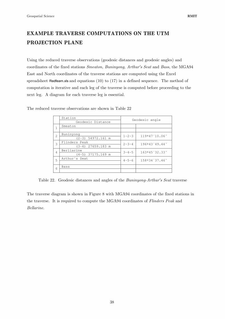
Using the reduced traverse observations (geodesic distances and geodesic angles) and
coordinates of the fixed stations Smeaton, Buninyong, Arthur's Seat and Bass, the MGA94
East and North coordinates of the traverse stations are computed using the Excel
spreadsheet Redfearn.xls and equations (10) to (17) in a defined sequence. The method of
computation is iterative and each leg of the traverse is computed before proceeding to the
next leg. A diagram for each traverse leg is essential.
The reduced traverse observations are shown in Table 22
Station Geodesic Distance
Geodesic angle
Smeaton 1 Buninyong 2 (2-3) 54972.161 m
1-2-3 119º47´10.06˝
Flinders Peak 3 (3-4) 27659.183 m
2-3-4 196º43´49.44˝
Berllarine 4 (4-5) 37175.169 m
3-4-5 163º45´32.33˝
Arthur's Seat 5
4-5-6 158º34´37.46˝
Bass 6
Table 22. Geodesic distances and angles of the Buninyong-Arthur's Seat traverse
The traverse diagram is shown in Figure 8 with MGA94 coordinates of the fixed stations in
the traverse. It is required to compute the MGA94 coordinates of Flinders Peak and
Bellarine.
38
Geospatial Science RMIT
LINE 1 Buninyong-Flinders Peak
.
. SMEATON 232 681.8995867 898.055
EN
BUNINYONG228 854.0415828 259.033
EN
273 741.5015796 490.265
EN
FLINDERS PEAK
β=
5°′
″
1217
39.88
θ =5°
′
″
1217
19.21
θ=
5°30
′″
5
6.99
L 54992.169
=
s 54972.161
=K 1.000 363 973
=
β°
′″
= 5
30 29.82
119 47 10.06° ′ ″
δ ″ = 20.67
δ ″ = 27.17
computed
1
2
3
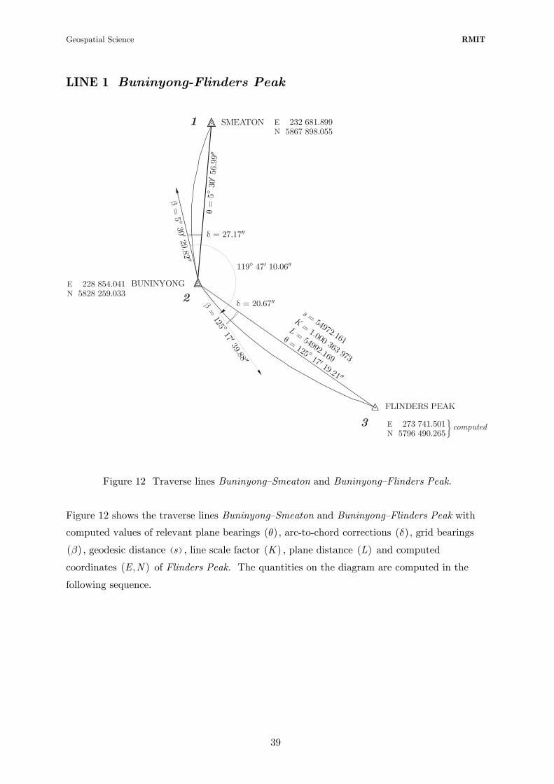
Figure 12 Traverse lines Buninyong–Smeaton and Buninyong–Flinders Peak.
Figure 12 shows the traverse lines Buninyong–Smeaton and Buninyong–Flinders Peak with
computed values of relevant plane bearings ( )θ , arc-to-chord corrections ( )δ , grid bearings
, geodesic distance (( )β )s , line scale factor ( , plane distance ( and computed
coordinates ( of Flinders Peak. The quantities on the diagram are computed in the
following sequence.
)K )L
),E N
39

Geospatial Science RMIT
STEP 1 Compute the plane bearing of the back-sight line Buninyong-Smeaton
Using the MGA94 coordinates from the traverse diagram (Figure 8) and equation (15) the
plane bearing θ of the line Buninyong-Smeaton is shown in Table 23
Station 1 MGA94 coordinates Station 2 MGA94
coordinates Plane Bearing
2-1
Buninyong 228854.041 E 5828259.033 N Smeaton 232681.899 E
5867898.055 N 5º30´56.99˝
Table 23. Plane bearing of the line Buninyong–Smeaton.
STEP 2 Compute the arc-to-chord correction of the back-sight line Smeaton–
Buninyong.
δ
The arc-to-chord correction is computed using equation (16). This equation requires the
mean radius 0mr k ρν= where and are computed for ρ ν ( )1 2 2mφ φ φ= + .
2.1 Use the Excel spreadsheet Redfearn.xls to convert MGA94 E,N coordinates of the
instrument station Buninyong, and back-sight station Smeaton, to GDA94 latitudes
and longitudes. The grid convergence γ and the Point Scale Factor k should also be
noted. The grid convergence is not used in these calculations but is computed from
Redfearn's formulae. The Point Scale Factor k of the instrument station is used as a
first approximation of the Line Scale Factor for the line Buninyong–Flinders Peak. The
computed values are shown in Table 24.
Station MGA94 coordinates
GDA94 coordinates
Grid convergence γ
Point Scale
Factor k
Buninyong 228854.041 E 5828259.033 N
-37º39´10.1563˝ 143º55´35.3835˝ -1º52´43.22˝ 1.000505669
Smeaton 232681.899 E 5867898.055 N
-37º17´49.7306˝ 143º59´03.1691˝
Table 24. MGA Zone 55 and GDA coordinates, grid convergence
and Point Scale Factor k of Buninyong and Smeaton.
γ
40

Geospatial Science RMIT
2.2 Calculate the mean latitude of the line Buninyong–Smeaton and use Redfearn.xls to
compute and . Then compute
mr
ρ ν 0mr k ρν= . Table 25 shows the computed values
with rounded to the nearest metre. mr
Radii of curvature Line (1-2) Mean latitude ρ ν
Mean radius
0mr k ρν=
1 Buninyong- 2 Smeaton -37º28´29.9434˝ 6359061.793 6386054.391 6369995
Table 25. Mean radius of the line Buninyong–Smeaton. mr
2.3 Calculate the arc-to-chord correction at Buninyong for the line Buninyong–Smeaton
using equation (16). Table 26 shows the computed value
Station 1 MGA94 coordinates Station 2 MGA94
coordinates mr arc-to-chord correction
1-2
Buninyong 228854.041 E 5828259.033 N Smeaton 232681.899 E
5867898.055 N 6369995 27.17˝
Table 26. Arc-to-chord correction at Buninyong for the line Buninyong–Smeaton.
STEP 3 Compute the grid bearing of the back-sight line Buninyong–Smeaton. β
The grid bearing of the line Buninyong–Smeaton is given by equation (17) using values in
Tables 23 and 26.
5 30 56.99 27.17 5 30 29.82β θ δ ′ ′′ ′′ ′= − = − = ′′
′′
STEP 4 Compute the grid bearing of the forward-sight line Buninyong–Flinders Peak. β
The grid bearing of the forward-sight is equal to the grid bearing of the back-sight plus the
geodesic angle at the instrument point from Table 22.
5 30 29.82 119 47 10.06 125 17 39.88β ′ ′′ ′ ′′ ′= + =
41

Geospatial Science RMIT
STEP 5 Compute the MGA94 E,N coordinates of Flinders Peak.
This step requires an iterative approach.
The first iteration is made as follows:
(1a) The grid bearing of the line Buninyong–Flinders Peak is assumed to be the plane
bearing . θ
(1b) The geodesic distance s of the line Buninyong–Flinders Peak, multiplied by the Point
Scale Factor k at Buninyong, is assumed to be the plane distance L.
(1c) Using these approximations for and L and plane trigonometry, approximate
coordinates of Flinders Peak are computed.
θ
The second iteration is made as follows:
(2a) Convert the approximate grid coordinates of Flinders Peak to latitudes and longitudes
using Redfearn.xls, calculate the mean latitude and the mean radius for the line
Buninyong–Flinders Peak as per steps 2.1 and 2.2 above. mr
(2b) Compute the arc-to-chord correction δ at Buninyong and the Line Scale Factor K for
the line Buninyong–Flinders Peak using equations (16) and (13).
(2c) Compute new values for the plane bearing and plane distance
then use plane trigonometry to compute new approximations of the coordinates of
Flinders Peak.
θ β δ= + L K s= ×
The third iteration is made as follows:
(3a) Compute the arc-to-chord correction δ at Buninyong and the Line Scale Factor L for
the line Buninyong–Flinders Peak using equations (16) and (13). The mean radius
computed in the second iteration can be used since its value, rounded to the nearest
metre, will not change. It is likely that the Line Scale Factor will remain unchanged.
mr
(3b) Compute new values for the plane bearing and plane distance
then use plane trigonometry to compute new approximations of the coordinates of
Flinders Peak.
θ β δ= + L K s= ×
The changes between the second and third iterations will generally be less than 1-2 mm.
The results of the iterative process are set out below.
42

Geospatial Science RMIT
5.1 First Iteration
Station 1 Plane Bearing 1-2
Plane Distance L K s= ×
Station 2
Buninyong 228854.041 E 5828259.033 N
125º17´39.88˝ s = 54972.161 K = 1.000505669 L = 54999.959
Flinders Peak 273744.675 E 5796481.266 N
Table 27. First approximation of MGA94 coordinates of Flinders Peak.
5.2 Second Iteration
Station MGA94 coordinates
GDA94 coordinates
Flinders Peak 273744.675 E 5796481.266 N
-37º57´03.9992˝ 144º25´29.6531˝
Table 28. Approximate MGA94 and GDA94 coordinates of Flinders Peak.
Radii of curvature Line (1-2) Mean latitude ρ ν
Mean radius
0mr k ρν=
1 Buninyong 2 Flinders Peak -37º48´07.0778˝ 6359415.132 6386172.668 6370231
Table 29. Approximate mean radius of the line Buninyong–Flinders Peak. mr
arc-to-chordStation 1 MGA94 coordinates Station 2 MGA94
coordinates mr L.S.F
-20.68˝ Buninyong 228854.041 E 5828259.033 N Flinders Peak 273744.675 E
5796481.266 N 6370231 1.000363963
Table 30. First approximations of arc-to-chord correction and Line
Scale Factor for the line Buninyong–Flinders Peak.
Station 1 Plane Bearing 1-2
Plane Distance L K s= ×
Station 2
Buninyong 228854.041 E 5828259.033 N
125º17´19.20˝ s = 54972.161 K = 1.000363963 L = 54992.169
Flinders Peak 273741.502 E 5796490.267 N
Table 31. Second approximation of MGA94 coordinates of Flinders Peak.
43
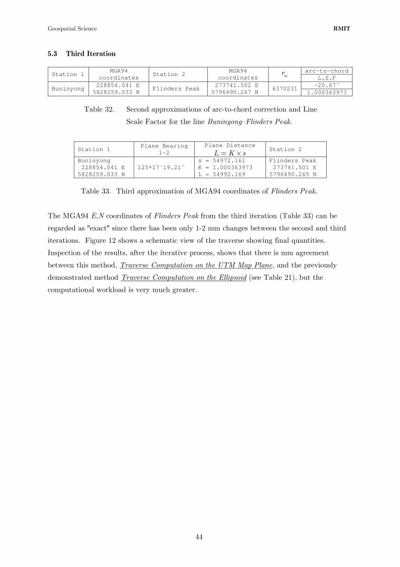
Geospatial Science RMIT
5.3 Third Iteration
arc-to-chordStation 1 MGA94 coordinates Station 2 MGA94
coordinates mr L.S.F
-20.67˝ Buninyong 228854.041 E 5828259.033 N Flinders Peak 273741.502 E
5796490.267 N 6370231 1.000363973
Table 32. Second approximations of arc-to-chord correction and Line
Scale Factor for the line Buninyong–Flinders Peak.
Station 1 Plane Bearing 1-2
Plane Distance L K s= ×
Station 2
Buninyong 228854.041 E 5828259.033 N
125º17´19.21˝ s = 54972.161 K = 1.000363973 L = 54992.169
Flinders Peak 273741.501 E 5796490.265 N
Table 33. Third approximation of MGA94 coordinates of Flinders Peak.
The MGA94 E,N coordinates of Flinders Peak from the third iteration (Table 33) can be
regarded as "exact" since there has been only 1-2 mm changes between the second and third
iterations. Figure 12 shows a schematic view of the traverse showing final quantities.
Inspection of the results, after the iterative process, shows that there is mm agreement
between this method, Traverse Computation on the UTM Map Plane, and the previously
demonstrated method Traverse Computation on the Ellipsoid (see Table 21), but the
computational workload is very much greater.
44

Geospatial Science RMIT
LINE 2 Flinders Peak–Bellarine
.
BELLARINE
BUNINYONG 228 854.0415828 259.033
EN
273 741.501
290 769.427
5796 490.265
5774 687.464
E
E
N
N
FLINDERS PEAK
196 43 49.44° ′ ″
δ ″ = 19.48
δ ″ = 12.22
computed4
2
3β
°′
″
= 142
00 49.17
θ
°′
″
= 305 17 19.21θ
°′
″
= 142
00 36.95
L = 27664.280
K =
1.000 184 278
s = 27659.183
β° ′
″
= 305 16 59.73
Figure 13 Traverse lines Flinders Peak–Buninyong and Flinders Peak–Bellarine.
Figure 13 shows the traverse lines Flinders Peak–Buninyong and Flinders Peak–Bellarine
with computed values of relevant plane bearings ( )θ , arc-to-chord corrections ( )δ , grid
bearings ( )β , geodesic distance ( )s , line scale factor ( , plane distance ( and computed
coordinates ( of Bellarine. The quantities on the diagram are computed in the same
sequence as set out for LINE 1 Buninyong–Flinders Peak and the abbreviated steps and
results are as follows.
)K )L
),E N
45

Geospatial Science RMIT
STEP 1 Compute the plane bearing of the back-sight line Flinders Peak–Buninyong
Station 1 MGA94 coordinates Station 2 MGA94
coordinates Plane Bearing
1-2
Flinders Peak 273741.501 E 5796490.265 N Buninyong 228854.041 E
5828259.033 N 305º17´19.21˝
Table 34. Plane bearing of the line Flinders Peak–Buninyong.
STEP 2 Compute the arc-to-chord correction of the back-sight line Flinders Peak–
Buninyong.
δ
2.1 Convert MGA94 E,N coordinates of the instrument station Flinders Peak, and back-
sight station Buninyong, to GDA94 latitudes and longitudes. The Point Scale Factor k
of the instrument station is used as a first approximation of the Line Scale Factor for
the line Flinders Peak–Bellarine.
Station MGA94 coordinates
GDA94 coordinates
Grid convergence γ
Point Scale
Factor k Flinders Peak
273741.501 E 5796490.265 N
-37º57´03.7047˝ 144º25´29.5333˝ -1º35´03.64˝ 1.000230557
Buninyong 228854.041 E 5828259.033 N
-37º39´10.1563˝ 143º55´35.3835˝
Table 35. MGA Zone 55 and GDA coordinates, grid convergence
and Point Scale Factor k of Flinders Peak.
γ
2.2 Calculate the mean latitude of the line Flinders Peak–Buninyong. mr
Radii of curvature Line (1-2) Mean latitude ρ ν
Mean radius
0mr k ρν=
1 Flinders Peak 2 Buninyong -37º48´06.9305˝ 6359415.088 6386172.654 6370231
Table 36. Mean radius of the line Flinders Peak–Buninyong. mr
Alternatively, use the value of the mean radius computed previously for the line
Buninyong–Flinders Peak (see Table 36). mr
46

Geospatial Science RMIT
2.3 Calculate the arc-to-chord correction at Flinders Peak for the line Flinders Peak–
Buninyong.
Station 1 MGA94 coordinates Station 2 MGA94
coordinates mr arc-to-chord correction
1-2 Flinders Peak
273741.501 E 5796490.265 N Buninyong 228854.041 E
5828259.033 N 6370231 19.48˝
Table 37. Arc-to-chord correction at Flinders Peak for the line Flinders Peak–Buninyong.
STEP 3 Compute the grid bearing of the back-sight line Flinders Peak–Buninyong. β
305 17 19.21 19.48 305 16 59.73β θ δ ′ ′′ ′′ ′= − = − = ′′
′′
STEP 4 Compute the grid bearing of the forward-sight line Flinders Peak–Bellarine. β
305 16 59.73 196 43 49.44 142 00 49.17β ′ ′′ ′ ′′ ′= + =
STEP 5 Compute the MGA94 E,N coordinates of Bellarine.
This step requires iteration.
5.1 First Iteration Compute approximate coordinates of Bellarine assuming the plane
bearing θ is the grid bearing β and line scale factor K is the point
scale factor k
Station 1 Plane Bearing 1-2
Plane Distance L K s= ×
Station 2
Flinders Peak 273741.501 E 5796490.265 N
142º00´49.17˝ s = 27659.183 K = 1.000230557 L = 27665.560
Bellarine 290768.923 E 5774685.447 N
Table 38. First approximation of MGA94 coordinates of Bellarine.
47
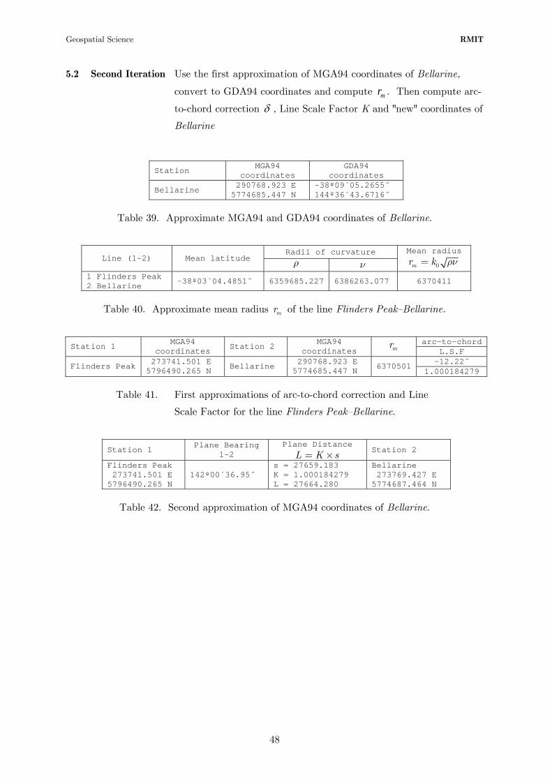
Geospatial Science RMIT
5.2 Second Iteration Use the first approximation of MGA94 coordinates of Bellarine,
convert to GDA94 coordinates and compute . Then compute arc-
to-chord correction mr
δ , Line Scale Factor K and "new" coordinates of
Bellarine
Station MGA94 coordinates
GDA94 coordinates
Bellarine 290768.923 E 5774685.447 N
-38º09´05.2655˝ 144º36´43.6716˝
Table 39. Approximate MGA94 and GDA94 coordinates of Bellarine.
Radii of curvature Line (1-2) Mean latitude ρ ν
Mean radius
0mr k ρν=
1 Flinders Peak 2 Bellarine -38º03´04.4851˝ 6359685.227 6386263.077 6370411
Table 40. Approximate mean radius of the line Flinders Peak–Bellarine. mr
arc-to-chordStation 1 MGA94 coordinates Station 2 MGA94
coordinates mr L.S.F
-12.22˝ Flinders Peak 273741.501 E 5796490.265 N Bellarine 290768.923 E
5774685.447 N 6370501 1.000184279
Table 41. First approximations of arc-to-chord correction and Line
Scale Factor for the line Flinders Peak–Bellarine.
Station 1 Plane Bearing 1-2
Plane Distance L K s= ×
Station 2
Flinders Peak 273741.501 E 5796490.265 N
142º00´36.95˝ s = 27659.183 K = 1.000184279 L = 27664.280
Bellarine 273769.427 E 5774687.464 N
Table 42. Second approximation of MGA94 coordinates of Bellarine.
48
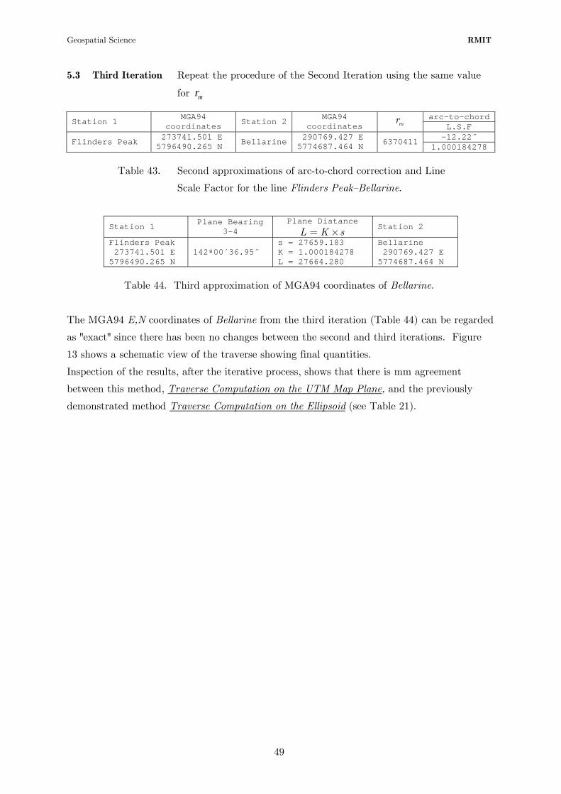
Geospatial Science RMIT
5.3 Third Iteration Repeat the procedure of the Second Iteration using the same value
for mr
arc-to-chordStation 1 MGA94 coordinates Station 2 MGA94
coordinates mr L.S.F
-12.22˝ Flinders Peak 273741.501 E 5796490.265 N Bellarine 290769.427 E
5774687.464 N 6370411 1.000184278
Table 43. Second approximations of arc-to-chord correction and Line
Scale Factor for the line Flinders Peak–Bellarine.
Station 1 Plane Bearing 3-4
Plane Distance L K s= ×
Station 2
Flinders Peak 273741.501 E 5796490.265 N
142º00´36.95˝ s = 27659.183 K = 1.000184278 L = 27664.280
Bellarine 290769.427 E 5774687.464 N
Table 44. Third approximation of MGA94 coordinates of Bellarine.
The MGA94 E,N coordinates of Bellarine from the third iteration (Table 44) can be regarded
as "exact" since there has been no changes between the second and third iterations. Figure
13 shows a schematic view of the traverse showing final quantities.
Inspection of the results, after the iterative process, shows that there is mm agreement
between this method, Traverse Computation on the UTM Map Plane, and the previously
demonstrated method Traverse Computation on the Ellipsoid (see Table 21).
49
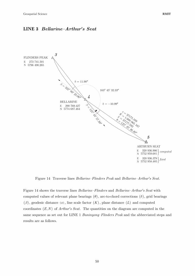
Geospatial Science RMIT
LINE 3 Bellarine–Arthur's Seat
.
BELLARINE
ARTHUR'S SEAT
273 741.501
290 769.427
320 936.906
320 936.378
5796 490.265
5774 687.464
5752 959.681
5752 958.485
E
E
E
E
N
N
N
N
FLINDERS PEAK
163 45 32.33° ′ ″
δ ″ = 11.90
δ − ″ = 10.99
computed
fixed
4
5
3
β
°′
″
= 322 00 25.06
β
°′
″
= 125
45 57.39
θ
°′
″
= 125 45 46.40
L = 37177.592
K = 1.000 065 167
s = 37175.169
Figure 14 Traverse lines Bellarine–Flinders Peak and Bellarine–Arthur's Seat.
Figure 14 shows the traverse lines Bellarine–Flinders and Bellarine–Arthur's Seat with
computed values of relevant plane bearings ( )θ , arc-to-chord corrections ( )δ , grid bearings
, geodesic distance (( )β )s , line scale factor ( , plane distance ( and computed
coordinates (
)K )L
),E N of Arthur's Seat. The quantities on the diagram are computed in the
same sequence as set out for LINE 1 Buninyong–Flinders Peak and the abbreviated steps and
results are as follows.
50

Geospatial Science RMIT
STEP 1 Compute the plane bearing of the back-sight line Bellarine–Flinders Peak
Station 1 MGA94 coordinates Station 2 MGA94
coordinates Plane Bearing
1-2
Bellarine 290769.427 E 5774687.464 N Flinders Peak 273741.501 E
5796490.265 N 322º00´36.95˝
Table 45. Plane bearing of the line Bellarine–Flinders Peak.
STEP 2 Compute the arc-to-chord correction of the back-sight line Bellarine–Flinders
Peak.
δ
2.1 Convert MGA94 E,N coordinates of the instrument station Bellarine, and back-sight
station Flinders Peak, to GDA94 latitudes and longitudes. The Point Scale Factor k of
the instrument station is used as a first approximation of the Line Scale Factor for the
line Bellarine–Arthur's Seat.
Station MGA94 coordinates
GDA94 coordinates
Grid convergence γ
Point Scale
Factor k
Bellarine 290769.427 E 5774687.464 N
-38º09´05.2005˝ 144º36´43.6944˝ -1º28´32.23˝ 1.000139186
Flinders Peak
273741.501 E 5796490.265 N
-37º57´03.7047˝ 144º25´29.5333˝
Table 46. MGA Zone 55 and GDA coordinates, grid convergence
and Point Scale Factor k of Bellarine.
γ
2.2 Calculate the mean latitude of the line Bellarine–Flinders Peak. mr
Radii of curvature Line (1-2) Mean latitude ρ ν
Mean radius
0mr k ρν=
1 Bellarine 2 Flinders Peak -38º03´04.4526˝ 6359685.217 6386263.074 6370411
Table 47. Mean radius of the line Bellarine–Flinders Peak. mr
Alternatively, use the value of the mean radius computed previously for the line Flinders
Peak–Bellarine (see Table 40). mr
51

Geospatial Science RMIT
2.3 Calculate the arc-to-chord correction at Bellarine for the line Bellarine–Flinders Peak.
Station 1 MGA94 coordinates Station 2 MGA94
coordinates mr arc-to-chord correction
1-2
Bellarine 290769.427 E 5774687.464 N
Flinders Peak
273741.501 E 5796490.265 N 6370411 11.90˝
Table 48. Arc-to-chord correction at Bellarine for the line Bellarine–Flinders Peak.
STEP 3 Compute the grid bearing of the back-sight line Bellarine–Flinders Peak. β
322 00 36.95 11.90 322 00 25.06β θ δ ′ ′′ ′′ ′= − = − = ′′
′
STEP 4 Compute the grid bearing of the forward-sight line Bellarine–Arthur's Seat. β
322 00 25.06 163 45 32.33 125 45 57.39β ′ ′′ ′ ′′ ′ ′= + =
STEP 5 Compute the MGA94 E,N coordinates of Arthur's Seat.
This step requires iteration.
5.1 First Iteration Compute approximate coordinates of Arthur's Seat assuming the
plane bearing θ is the grid bearing β and line scale factor K is the
point scale factor k
Station 1 Plane Bearing 1-2
Plane Distance L K s= ×
Station 2
Bellarine 290768.923 E 5774685.447 N
125º45´57.39˝ s = 37175.169 K = 1.000139186 L = 37180.343
Arthur's Seat 320937.981 E 5752956.466 N
Table 49. First approximation of MGA94 coordinates of Arthur's Seat.
52

Geospatial Science RMIT
5.2 Second Iteration Use the first approximation of MGA94 coordinates of Arthur's Seat,
convert to GDA94 coordinates and compute . Then compute arc-
to-chord correction mr
δ , Line Scale Factor K and "new" coordinates of
Arthur's Seat
Station MGA94 coordinates
GDA94 coordinates
Arthur's Seat 320937.981 E 5752956.466 N
-38º21´13.1930˝ 144º57´02.6191˝
Table 50. Approximate MGA94 and GDA94 coordinates of Arthur's Seat.
Radii of curvature Line (1-2) Mean latitude ρ ν
Mean radius
0mr k ρν=
1 Bellarine 2 Arthur's Seat -38º15´09.1968˝ 6359903.785 6386336.234 6370557
Table 51. Approximate mean radius of the line Bellarine–Arthur's Seat. mr
arc-to-chordStation 1 MGA94 coordinates Station 2 MGA94
coordinates mr L.S.F
-11.00˝ Bellarine 290769.427 E 5774687.464 N Arthur's Seat 320937.981 E
5752956.466 N 6370557 1.000065164
Table 52. First approximations of arc-to-chord correction and Line
Scale Factor for the line Bellarine–Arthur's Seat.
Station 1 Plane Bearing 1-2
Plane Distance L K s= ×
Station 2
Bellarine 290769.427 E 5774687.464 N
125º45´46.39˝ s = 37175.169 K = 1.000065164 L = 37177.591
Arthur's Seat 320936.907 E 5752959.684 N
Table 53. Second approximation of MGA94 coordinates of Arthur's Seat.
53

Geospatial Science RMIT
54
5.3 Third Iteration Repeat the procedure of the Second Iteration using the same value
for mr
arc-to-chordStation 1 MGA94 coordinates Station 2 MGA94
coordinates mr L.S.F
-10.99˝ Bellarine 290769.427 E 5774687.464 N Arthur's Seat 320936.907 E
5752959.684 N 6370557 1.000065167
Table 54. Second approximations of arc-to-chord correction and Line
Scale Factor for the line Bellarine–Arthur's Seat.
Station 1 Plane Bearing 1-2
Plane Distance L K s= ×
Station 2
Bellarine 290769.427 E 5774687.464 N
125º45´46.40˝ s = 37175.169 K = 1.000065167 L = 37177.592
Arthur's Seat 320936.906 E 5752959.681 N
Table 55. Third approximation of MGA94 coordinates of Arthur's Seat.
The MGA94 E,N coordinates of Arthur's Seat from the third iteration (Table 55) can be
regarded as "exact" since there has only mm changes between the second and third iterations.
Figure 14 shows a schematic view of the traverse showing final quantities.
Inspection of the results, after the iterative process, shows that there is mm agreement
between this method, Traverse Computation on the UTM Map Plane, and the previously
demonstrated method Traverse Computation on the Ellipsoid (see Table 21).