On the Linear Independence of Multivariate i?-Splines. II ......On the Linear Independence of...
21
mathematics of computation volume 41, number 163 july 1983. pages 143-163 On the Linear Independence of Multivariate i?-Splines. II: Complete Configurations By Wolfgang A. Dahmen and Charles A. Micchelli Abstract. The first part of this paper is concerned with global characterizations of both the multivariate ß-spline and the multivariate truncated power function as smooth piecewise polynomials. In the second part of the paper we establish combinatorial criteria for the linear independence of multivariate ß-splines corresponding to certain configurations of knot sets. 1. Introduction. A characteristic feature of the univariate ß-spline is the well-known fact that it has minimal support among all splines of a fixed degree having the requisite smoothness conditions determined by the multiplicities of its corresponding knots. In particular, for any set of distinct knots x0< xx < ■ ■ ■< xn, there is (up to a multiplicative constant) a unique function (.ß-spline) which is supported on (x0, xn), has n — 2 continuous derivatives everywhere and on each interval (Xj, xj+, ), 0 < jr < n — 1, is a polynomial of degree < n — 1. This function has an explicit representation as a divided difference (1.1) M(t\x0,...,x„) = /_ lX, [■*()>•••»*«]( ° -')+"' and can be seen to have exactly n — 1 knots xx,...,xn_x interior to its interval of support (xn, xn). It is this latter fact that characterizes M(t) as having minimal support. For there is no (nontrivial) function sharing the same properties as M but having one less knot in its support. These remarkable properties of the univariate ß-spline (minimal support and the representation (1.1)) are due to Curry and Schoenberg [4], One of us has already provided a multivariate version of (1.1) by using multi- variate ß-splines and truncated powers [5]. However, the analog of the minimal support property of the univariate ß-spline has yet to be settled in higher dimen- sions. The piecewise polynomial nature of the multivariate ß-spline is known to be much more complicated than in the univariate case. Thus it may be somewhat surprising that a global characterization of the multivariate ß-spline is indeed valid. One of our objectives is to prove such a result. Furthermore, by characterizing the restriction of the multivariate truncated power function to hyperplanes, we are able to establish a similar result for this density function as well. The second and main objective of this paper is to use these results to establish some combinatorial criteria for the linear independence of multivariate ß-splines corresponding to certain configurations of knots. We have already treated this Received July 21, 1981; revised April 26, 1982. 1980Mathematics Subject Classification. Primary 41A63; Secondary 41A05, 41A15, 05B99. ©1983 American Mathematical Society 0025-5718/82/0O0O-1241 /$04.75 143 License or copyright restrictions may apply to redistribution; see https://www.ams.org/journal-terms-of-use
Transcript of On the Linear Independence of Multivariate i?-Splines. II ......On the Linear Independence of...

mathematics of computationvolume 41, number 163july 1983. pages 143-163
On the Linear Independence of Multivariate
i?-Splines. II: Complete Configurations
By Wolfgang A. Dahmen and Charles A. Micchelli
Abstract. The first part of this paper is concerned with global characterizations of both the
multivariate ß-spline and the multivariate truncated power function as smooth piecewise
polynomials. In the second part of the paper we establish combinatorial criteria for the linear
independence of multivariate ß-splines corresponding to certain configurations of knot sets.
1. Introduction. A characteristic feature of the univariate ß-spline is the well-known
fact that it has minimal support among all splines of a fixed degree having the
requisite smoothness conditions determined by the multiplicities of its corresponding
knots. In particular, for any set of distinct knots x0< xx < ■ ■ ■ < xn, there is (up to
a multiplicative constant) a unique function (.ß-spline) which is supported on
(x0, xn), has n — 2 continuous derivatives everywhere and on each interval (Xj, xj+, ),
0 < jr < n — 1, is a polynomial of degree < n — 1. This function has an explicit
representation as a divided difference
(1.1) M(t\x0,...,x„) = /_ lX, [■*()>•••»*«]( ° -')+"'
and can be seen to have exactly n — 1 knots xx,...,xn_x interior to its interval of
support (xn, xn). It is this latter fact that characterizes M(t) as having minimal
support. For there is no (nontrivial) function sharing the same properties as M but
having one less knot in its support. These remarkable properties of the univariate
ß-spline (minimal support and the representation (1.1)) are due to Curry and
Schoenberg [4],
One of us has already provided a multivariate version of (1.1) by using multi-
variate ß-splines and truncated powers [5]. However, the analog of the minimal
support property of the univariate ß-spline has yet to be settled in higher dimen-
sions. The piecewise polynomial nature of the multivariate ß-spline is known to be
much more complicated than in the univariate case. Thus it may be somewhat
surprising that a global characterization of the multivariate ß-spline is indeed valid.
One of our objectives is to prove such a result. Furthermore, by characterizing the
restriction of the multivariate truncated power function to hyperplanes, we are able
to establish a similar result for this density function as well.
The second and main objective of this paper is to use these results to establish
some combinatorial criteria for the linear independence of multivariate ß-splines
corresponding to certain configurations of knots. We have already treated this
Received July 21, 1981; revised April 26, 1982.
1980 Mathematics Subject Classification. Primary 41A63; Secondary 41A05, 41A15, 05B99.
©1983 American Mathematical Society
0025-5718/82/0O0O-1241 /$04.75
143
License or copyright restrictions may apply to redistribution; see https://www.ams.org/journal-terms-of-use

144 WOLFGANG A. DAHMEN AND CHARLES A. MICCHELLI
question to some degree in [8] (cf. also [13]), where certain collections of ß-splines
were studied. However, the arguments which insure the linear independence of the
corresponding ß-splines involve, among other things, some restrictions on the knot
positions, which, although being necessary for the stability of the basis, do not seem
to be essential for their linear independence.
Our objective is therefore to explore the connections between linear dependencies
of ß-splines and purely combinatorial properties of the corresponding configurations
of knot sets. To this end, we shall, for instance, determine the dimension of the span
of ß-splines associated with what we call a complete configuration. (This terminol-
ogy comes from the fact that the complete configuration for a set of affinely
independent points in the plane is the complete graph whose vertices are these
points.) Furthermore, our results will allow us to remove the above mentioned
restrictions on the knot configurations considered in [8], [13].
Finally, we mention that there is a direct relationship between linearly indepen-
dent ß-splines and certain classes of multivariate rational functions. This fact will be
explained fully later. We also mention in this context that we are able to give a
simpler proof of some recent results of Hakopian [12] on multivariate divided
differences and interpolation.
2. A Global Characterization of the Multivariate ß-Spline. A central objective of
this section is to point out in what sense the multivariate ß-spline and related
functions have minimal support.
Let us start by fixing some notation and summarizing a few known facts for later
reference.
Elements of the Euclidean space Rs will be denoted by x, u, z, x — (xx,...,xs).
XA(x),[A],vols(A), \A\ will denote the indicator function, the (closed) convex hull,
the s-dimensional Lebesgue measure and, in case A is finite, the cardinality (count-
ing multiplicities) of a given set A, respectively. The restriction of a given function/:
Rs -» R to some subset A C Rs will be indicated by /|^. In particular, when A is an
affine subspace of Rs,f\A will be always considered as a function of correspondingly
fewer variables with respect to a suitable coordinate system for A. Adopting the
standard multi-index notation for a, ß G Z+ , i.e. | a \ — ax + • • • +as, xa = jcf '
• • • x"1, we define the s-variate polynomials of (total) degree < k as usual by
n*,,= ( 2 caxa:caER,xeR°).1 \a\<k >
Let T be any collection of (s — l)-dimensional sets in Rs. TLk S(T) will then mean
the class of all (s-varíate) functions/ such that/|D G Uk s for any region D which is
not intersected by any element of T.
We shall sometimes refer to any (s — l)-dimensional set p in Rs such that in a
neighborhood of some point of p, /is in Uk s on each side of p (but not in IIks in the
neighborhood) as a cut region for /. The set of all cut regions of a given function /
will be denoted by T(f), and clearly T(f) C T whenever/ £ nti(r).
A knot set K = {x°,...,x"} C Rs, n>s, will always be assumed to satisfy
vol5([AT]) > 0. Let us emphasize here that in our notation \K\= n + 1, even though
K may contain fewer than n + 1 distinct vectors.
License or copyright restrictions may apply to redistribution; see https://www.ams.org/journal-terms-of-use
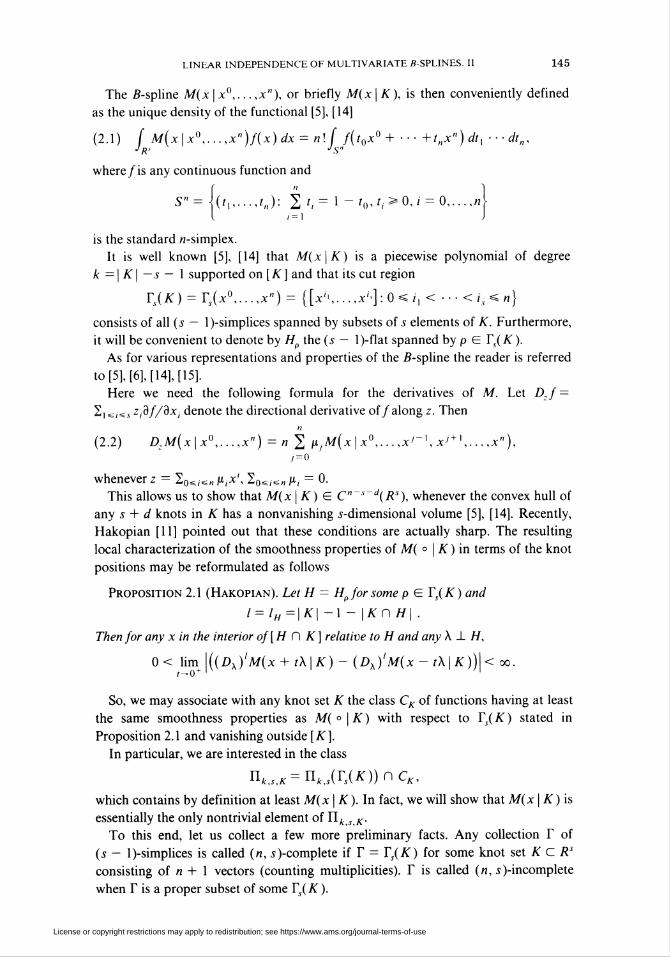
LINEAR INDEPENDENCE OF MULTIVARIATE B-SPLINES. II 145
The ß-spline M(x\x°,...,x"), or briefly M(x\K), is then conveniently defined
as the unique density of the functional [5], [14]
(2.1) ( M(x\x°,...,x")f(x)dx = n\f f(t0x° + ■■■ +t„xn)dtx ■■•dt„,JR, Js„
where /is any continuous function and
S"=Utx,...,tn): £:,= l-io,//>0,i = 0,...,«J
is the standard «-simplex.
It is well known [5], [14] that M(x\K) is a piecewise polynomial of degree
k = | K | — 5 — 1 supported on [ K ] and that its cut region
TS(K) = Ts(x°,...,xn) = {[jc\...,je'']:0<i, < •■• </,<«}
consists of all (s — l)-simplices spanned by subsets of s elements of K. Furthermore,
it will be convenient to denote by Hp the (s — l)-flat spanned by p G TS(K).
As for various representations and properties of the ß-spline the reader is referred
to [5], [6], [14], [15].
Here we need the following formula for the derivatives of M. Let Dzf =
2i«,<i zfif/dx, denote the directional derivative of/along z. Then
n
(2.2) DzM(x\x°,...,x") = n 2 PjM(x\x°.xJ~\ xi+x,...,x"),v-o
whenever z = 20aS/s:„ p,x', 20<i<„ p¡ = 0.
This allows us to show that M(x\K) G C"~s~d(Rs), whenever the convex hull of
any s + d knots in K has a nonvanishing s-dimensional volume [5], [14]. Recently,
Hakopian [11] pointed out that these conditions are actually sharp. The resulting
local characterization of the smoothness properties of M( ° \ K ) in terms of the knot
positions may be reformulated as follows
Proposition 2.1 (Hakopian). Let H = Hpfor some a G Ys(K)and
l = l„=\K\-\-\Kf\H\.
Then for any x in the interior of[H D K ] relative to H and any \ ± H,
0< liia\((Dx)'M(x + t\\K)- (Dx)'M(x - t\\K))\< oo.
So, we may associate with any knot set K the class CK of functions having at least
the same smoothness properties as M( ° \ K ) with respect to Ts( K ) stated in
Proposition 2.1 and vanishing outside [K].
In particular, we are interested in the class
which contains by definition at least M(x\K). In fact, we will show that M(x \ K) is
essentially the only nontrivial element of n¿ s K.
To this end, let us collect a few more preliminary facts. Any collection T of
(s - l)-simplices is called (n, incomplete if T = TS(K) for some knot set K C Rs
consisting of « + 1 vectors (counting multiplicities). T is called (n, j)-incomplete
when T is a proper subset of some T^ K ).
License or copyright restrictions may apply to redistribution; see https://www.ams.org/journal-terms-of-use
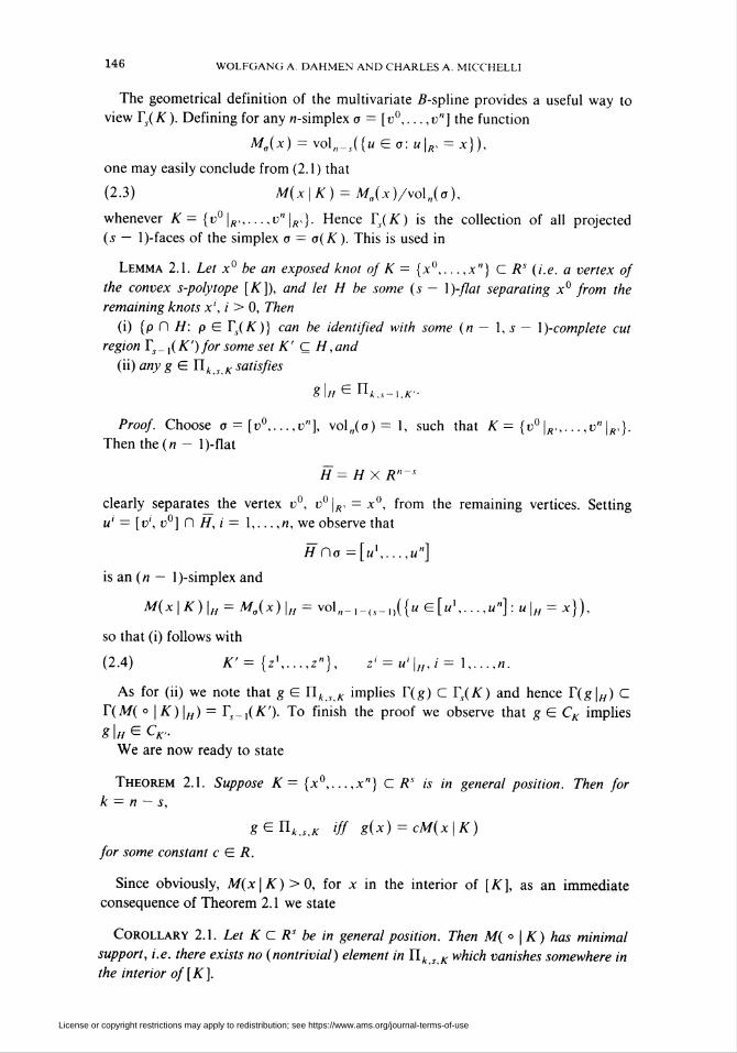
146 WOLFGANG A. DAHMEN AND CHARLES A. MICCHELLI
The geometrical definition of the multivariate ß-spline provides a useful way to
view rs(A"). Defining for any «-simplex a = [v°,...,v"] the function
Ma(x) =vol„_1.({«Ea: u\R, = x}),
one may easily conclude from (2.1) that
(2.3) M(x\K) = M„(x)/vo\n(o),
whenever K = {v° \R.,.. .,v" \R,}. Hence TS(K) is the collection of all projected
(s — l)-faces of the simplex a = a(K). This is used in
Lemma 2.1. Let x° be an exposed knot of K = {x0,... ,x"} C Rs (i.e. a vertex of
the convex s-polytope [K]), and let H be some (s — \)-flat separating x° from the
remaining knots x', i > 0, Then
(i) {p n H: p G TS(K)} can be identified with some (n — 1, s — \)-complete cut
region Is_ x( K') for some set K' C H, and
(ii) any g El If k sK satisfies
g¡HElík,s-i.K-
Proof. Choose a = [v0,... ,vn], vol„(o) = 1, such that K = {t>° \R„... ,v" \R,}.
Then the (n - l)-flat
H = H X R"'"
clearly separates the vertex v°, v° \R, = x°, from the remaining vertices. Setting
u' = [v1, v°] n H, i — 1,... ,n, we observe that
HDo =[«■,...,«"]
is an ( n — l)-simplex and
M(x\K)\H = M0(x)\fi = vol„_x_(s_X){{u<=[ui,...,un]:u\H = x}),
so that (i) follows with
(2.4) K'={zl.z"), z' = u'\H,i= \,...,n.
As for (ii) we note that g G IlksK implies 1(g) C IS(K) and hence I(g\H) C
I(M( ° \K)\H) = IS_X(K'). To finish the proof we observe that g G CK implies
g|//G Or-We are now ready to state
Theorem 2.1. Suppose K= {x°,...,x"} C Rs is in general position. Then for
k = n — s,
?enUJÎ iff g(x) = cM(x\K)
for some constant c G R.
Since obviously, M(x\K) > 0, for x in the interior of [Ä"], as an immediate
consequence of Theorem 2.1 we state
Corollary 2.1. Let K C Rs be in general position. Then M(° \K) has minimal
support, i.e. there exists no (nontrivial) element in IfksK which vanishes somewhere in
the interior of[K].
License or copyright restrictions may apply to redistribution; see https://www.ams.org/journal-terms-of-use
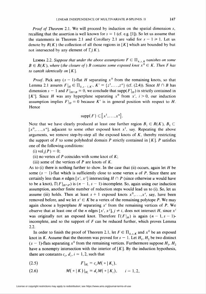
LINEAR INDEPENDENCE OF MULTIVARIATE B-SPLINES. II 147
Proof of Theorem 2.1. We will proceed by induction on the spatial dimension s,
recalling that the assertion is well known for s — 1 (cf. e.g. [1]). So let us assume that
the statements in Theorem 2.1 and Corollary 2.1 are valid for s — 1 > 1. Let us
denote by R(K) the collection of all those regions in [K] which are bounded by but
not intersected by any element of rs(A").
Lemma 2.2. Suppose that under the above assumptions F G Uk 5 K vanishes on some
B G R(K), where (the closure of) B contains some exposed knot x° G A". Then F has
to vanish identically on [K].
Proof. Pick any (s — l)-flat H separating x° from the remaining knots, so that
Lemma 2.1 assures F\H G HktS-X,K; K' = (z',...,z"} (cf. (2.4)). Since HOB has
dimension s — 1 and F\HnB — 0, we conclude that supp(F|w) is strictly contained in
\K'\. Since H was any hyperplane separating x° from x', i > 0, our induction
assumption implies F\H = 0 because K' is in general position with respect to H.
Hence
supp(F) c[x'.x"].
Note that we have clearly produced at least one further region ß, G R(K), Bx C
[x0,...,xn], adjacent to some other exposed knot x1, say. Repeating the above
arguments, we remove step-by-step all the exposed knots of K, thereby restricting
the support of F to some polyhedral domain P strictly contained in [K], P satisfies
one of the following conditions:
(i)vo\s(P) = 0;
(ii) no vertex of P coincides with some knot of K;
(iii) some of the vertices of P are knots of A".
As to (i) there is nothing further to show. In the case that (ii) occurs, again let H be
some (s — l)-flat which is sufficiently close to some vertex u of P. Since there are
certainly less than n edges [x', xJ] intersecting H n P (since otherwise u would have
to be a knot), Y(F\HnP) is (n — 1, s — 1 )-incomplete. So, again using our induction
assumption, another finite number of reduction steps would lead us to (i). So, let us
assume (iii) holds. Then at least 5 + 1 exposed knots x°,...,xJ, say, have been
removed before, and we let x' G K be a vertex of the remaining poly tope P. We may
again choose a hyperplane H separating x' from the remaining vertices of P. We
observe that at least one of the n edges [x', xJ],j =£ i, does not intersect H, since x'
was originally not an exposed knot. Therefore I(F\H) is again (n — l, s — 1)-
incomplete, and so the support of F can be reduced further, which proves Lemma
2.2.
In order to finish the proof of Theorem 2.1, let F G HktS<¡( and x° be an exposed
knot in K. Assume that the theorem was proved for s — 1. Let Hx, H2 be two distinct
(s — l)-flats separating x° from the remaining vertices. Furthermore suppose Hx, H2
have a nonempty intersection with the interior of [A"]. By the induction hypothesis,
there are constants c„ d¡, i = 1,2, such that
(2-5) F\H=c,M(o\Ki),
(2.6) M(o\K)\H=diM(o\Ki), i =1,2,
License or copyright restrictions may apply to redistribution; see https://www.ams.org/journal-terms-of-use

148 WOLFGANG A. DAHMEN AND CHARLES A. MICCHELLI
where K, = H, n {[x°, x1],... ,[x°, x"]}, ; = 1,2, and dx, d2 are nonzero. Choosing
a constant a such that adx = cx, then F — aM( ° | A) clearly vanishes on Hx. On the
other hand, since H2 intersects Hx and
(2.7) (F - aM( o | A)) \,h = (c2 - ad2)M( o | A2),
F — aM( ° | A) also vanishes on H2. Since a actually did not depend on H2, we infer
from (2.7) that
(F-aM(°\K))\B = 0
for some region B E R(K) where ß is adjacent to x°. Clearly F — a/Vf( ° | A) G
nfciJiJf, and so Lemma 2.2 confirms
F- aM(°\K) = 0 on[A],
which finishes the proof of Theorem 2.1.
In order to derive analogous results for multivariate truncated powers as well, it is
useful to introduce the following more general class of density functions.
For a given u: R — R and x',... ,xv G Rs we define Gu(x | x\... ,xm) formally by
requiring that [7]
(2.8) / • • • / «(/, + -.. +tjf(txx] + ■■■ +tmxm) dtx-- dtm
f Gu(x\xx,...,x"')f(x)dxJot
holds for any locally supported continuous function/on R\
The close connection between Gu and the ß-spline is revealed by the following
relation [7]
(2.9) Gu(x|x',...,xm) = r°w(A)«m-,~1M(/r1x|x,,...,xm)-'o
dh.
We are mainly interested in the following choices of <o [7]: ^,(0 = X[o,i](0<
w2(i) = 1, u3(t) = e~'. In fact, in the first case we simply have [7] Gu(, ° | x'.xm)
= (\/m\)M( ° | 0, xl,...,xm), whereas w2 gives rise to the multivariate truncated
powers [5], [15] which will be henceforth briefly denoted by G(° |x',...,xm).
However, in order to make sure that (2.8) makes sense in this case, we have to
impose the following conditions on the directions {x'}:
(2.10) 0 e[x',...,xm].
It is known [5] that G( ° \ x\... ,xm) is a piecewise polynomial of degree m — s
with support
(x',...,xm)+= 2 tjx':tj>0,j= l,...,w
and cut regions
rj°(x',...,xm) = {(x\...,x'-)+ : 1 </, < ■••</,_, <m}.
Furthermore, let H be any (s - l)-flat inl°(xx,.. .,xm). Setting
(2.11) l = m-\-\Hn{x1,...,xm}\,
License or copyright restrictions may apply to redistribution; see https://www.ams.org/journal-terms-of-use

LINEAR INDEPENDENCE OF MULTIVARIATE S-SPLINES. II 149
the /th order derivatives of G( ° | x1.xm) are known to have finite jumps across
H [5]. The same cut regions and smoothness properties are obtained for the third
choice w3(0 [7]. In this case
(2.12) A(x|x'.xm) = GUf(x\xl..v'")
turns out to be a piecewise exponential function (where no restrictions on the
directions (x'} are required).
A useful link between functions of the above type and their univariate counter-
parts is conveniently expressed by means of the Radon transform (cf. [10]) which is
defined for/ G LX(RS) by
(Rf)(X,t)=f f(x)dx, AGßs= (vGA- \\y\\ = 1},Jx\ = t
where ||_y|| = (y-y)x/1 and x-y denotes the standard inner product on Rs. Conse-
quently one has the identity [14]
(RM( o |x°,...,x"))(a,0 = M(/|A-x°,...,A-x"),
i.e. the Radon transform maps multivariate ß-splines into univariate ones.
Similarly we obtain
Lemma 2.3. For any ÂËÛ, let Hx , = {x G AJ: x • A = r}, and let G and A be
defined as above.
(i) Suppose x',...,xm satisfy (2.10) and ˣfis is chosen so that Hx t D
(x',...,x"') + is bounded for any t > 0. Then one has
(RG{o\xx,...,x"))(\,t)= f[\-xÁ i-T1-
(ii)(RA(o\xx,...,xm))(\,t) = (Ex* ■■■ *EJ(t), El(t) = t%e-Xx'!, where td+
= X/?+(0'i/ and " * " denotes convolution.
Proof, (i): Suppose g: R -> R has local support. Note that then supp(g(A-x)) n
(x1,.. - ,xm>+ is bounded by assumption, so that we may write (cf. (2.8))
/•OO y>00 .
/ •••/ g(tx\-xx + ---+tm\-xm)dtx---dtm
= ( G(x\xx,...,xm)g(X-x)dx.JRS
Since [2], [7]
r r00
(2.13) f(x)g(\-x)dx= (Rf)(X,t)g(t)dt,JRS •'-oo
the right-hand side of the previous equation reads
f{RG{o\xx,...,xm))(X,t)g(t)dt.
License or copyright restrictions may apply to redistribution; see https://www.ams.org/journal-terms-of-use

150 WOLFGANG A. DAHMEN AND CHARLES A. MICCHELLI
Assertion (i) follows then from the equality
r---rg{txx-xx + ---+tmx-xm)dtx---dtnJo Jo
= fU*y fRt:-xg(t)dt..y=i
As to (ii) it is not hard to prove that
(2.14) j A(x\x\...,xm)e-Xxdx = Ml (1 + \-xJ)\
holds for Re(A-xy) > -1. Thus (2.13) again yields
/(aa(° I jc1,. .. ,jcm))(X, /)e-* dSf = Ü (1 +A-JC-0) ■
On the other hand we know that (1 + A-x^)"1 = lRt%e~Kx''e~'dt, whence the
assertion readily follows.
We are now in the position to state the precise relation between truncated powers
and lower-dimensional ß-splines.
Theorem 2.2. Suppose 0 G [x',...,x"'] and every s of the vectors x' span Rs.
Furthermore suppose that ˣn5 has been chosen so that HXt D (x1,... ,xm>+ is
bounded. Then
I m \-'
G{o\xl,...,xm)\Hx=\ R\-xA trXM(°\z\...,zm),\j=\ I
where z' = HXt n {rx': r^O}, i = 1,... ,m.
Proof. Choosing z' as above, we clearly have for F = G( ° | x1,... ,xm) \H
supp(F) = HXJ n (x1,...,xm>+ =[z\...,zm].
Moreover, A' = (z1,... ,zm) is in general position (with respect to Hx ,) and
rJ°(x',..,x")|„x/ = r(F) = rJ_,(A').
Recalling the smoothness properties of the ß-spline (Proposition 2.1) and those of
the truncated powers (2.11) we conclude
•^ £= I*-m-s,s-\,K'•
Hence Theorem 2.1 implies
F(x) = cM(x\K'), xEHx„
for some c G R. In order to determine the constant c, we recall that jRS M(x \ A ) dx
= 1, so that one obtains, in view of the definition of the Radon transform,
c=f cM(z\zx,...,zm)dz= f G(z\xx,...,xm)dz•V, -V,
= {RG(°\x\..,,xm))(\,t)= n *-xA t™-\
where we have used Lemma 2.3(i) in the last equality.
License or copyright restrictions may apply to redistribution; see https://www.ams.org/journal-terms-of-use
LINEAR INDEPENDENCE OF MULTIVARIATE S-SPLINES. II 151
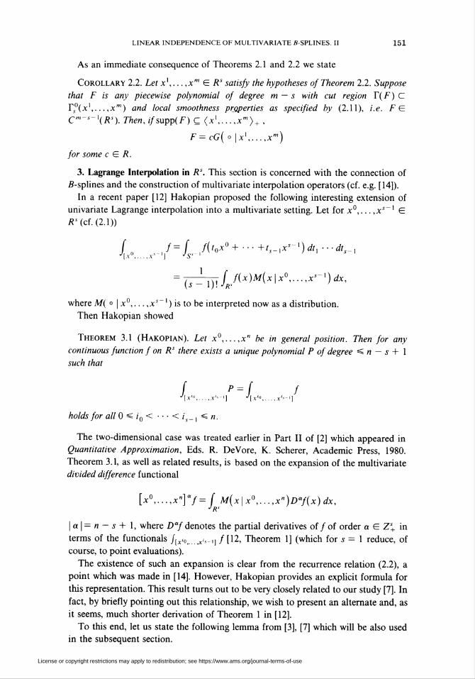
As an immediate consequence of Theorems 2.1 and 2.2 we state
Corollary 2.2. Let xx,...,xm G Rs satisfy the hypotheses of Theorem 2.2. Suppose
that F is any piecewise polynomial of degree m — s with cut region 1(F) C
I°(xx,.. .,xm) and local smoothness properties as specified by (2.11), i.e. F G
C'-S~X(RS). Then, if supp(F) C (x',...,xm>+ ,
F=cG(° |x',...,xm)
for some c G R.
3. Lagrange Interpolation in Rs. This section is concerned with the connection of
ß-splines and the construction of multivariate interpolation operators (cf. e.g. [14]).
In a recent paper [12] Hakopian proposed the following interesting extension of
univariate Lagrange interpolation into a multivariate setting. Let for x0,... ,xJ~' G
A* (cf. (2.1))
/o ,/ = / ,/('o*0 + ---+',-i*'~1)<*i ■••*,-!•'[.v0.x'-'] ¿S'-*
= , l u. [ f{x)M(x\x°,...,x°-x)dx,(s - I)! JR>
where M( o | x0,... ,xs~') is to be interpreted now as a distribution.
Then Hakopian showed
Theorem 3.1 (Hakopian). Let x°,...,x" be in general position. Then for any
continuous function f on Rs there exists a unique polynomial P of degree < n — s + 1
such that
/ '=/ /J[x"'.x1'-'] •'[jc'o.x'»-i]
holds for allO*siin< ••• < is-, « n.
The two-dimensional case was treated earlier in Part II of [2] which appeared in
Quantitative Approximation, Eds. R. DeVore, K. Scherer, Academic Press, 1980.
Theorem 3.1, as well as related results, is based on the expansion of the multivariate
divided difference functional
[x°,...,x"]7= f M(x\x°,...,xn)Daf(x)dx,JRS
I a | = n — s + 1, where Daf denotes the partial derivatives of / of order a £ Z'+ in
terms of the functionals f[x,0 xis-t] /[12, Theorem 1] (which for s = 1 reduce, of
course, to point evaluations).
The existence of such an expansion is clear from the recurrence relation (2.2), a
point which was made in [14]. However, Hakopian provides an explicit formula for
this representation. This result turns out to be very closely related to our study [7]. In
fact, by briefly pointing out this relationship, we wish to present an alternate and, as
it seems, much shorter derivation of Theorem 1 in [12].
To this end, let us state the following lemma from [3], [7] which will be also used
in the subsequent section.
License or copyright restrictions may apply to redistribution; see https://www.ams.org/journal-terms-of-use

152 WOLFGANG A. DAHMEN AND CHARLES A. MICCHELLI
Lemma 3.1. Suppose 0, x°,...,x" G Rs are in general position and let for any
IE {0,..., n), \I\— s, x' be the unique solution of \ + xJ■ x' = 0, y G /. Then every
polynomial of total degree *£ n + 1 — 5 can be expanded as
Q(x)= 2 Q(x>)Q,(x),\r\=s
and the polynomials Q,(x) = IIyS/(l + x-xJ)/(\ + x'-xj) satisfy Q¡(xJ) = 8,j,
I,JE {0,...,«}, |/| = |/|= j.
Now let qm(x) be any homogeneous polynomial of degree m and qm(D) the
associated differential operator. In view of (2.2) we can find coefficients pj,
J E {0,...,«}, such that for smoothg: R -> R and A = {x°.x") E Rs
(3.1) f qm(D)M(x\K)g'"'m\z-x)dx
= 2 Pjf g("~m)(z-x)M{x\K\{x':jEJ})dx.
Integration by parts applied to the left-hand side of (3.1) readily yields the divided
difference
n\(-\)mqm(z)[z-x°,...,z-x"]g.
Similarly the right-hand side of (3.1) can be rewritten as
(n-m)\ 2 *»/[*■ {K\{x^:jEJ})]g.\J\ = m
In particular we may choose g(t) = 1/(1 + /), which provides
/ -' W*)/ft (!+*•*')= 2 Pj/WÜ+zxJ)\n m>- 7 = 0 \J\ = m jdJ
and hence
(3.2) u;) = (":,m)! 2 ii/ii(i+*-*y)|/| = m jEJ
(which is easily seen to be equivalent to (3.1) by the denseness of the span of the
1/(1 + at), a G C). Choosing now m = n + 1 — s, we obtain
9n+1-í(-) = íi^7i11 2 e,no+*-*').\J\=n+\-s j<EJ
which we write in the equivalent form
= i^7111 2 i/II0 + *^).\I\=s j&]
But Lemma 3.1 then says that the coefficients tj, are uniquely determined. In
particular, when qn+x_s(x) = x", | a |= n + 1 — s, combining (3.1) with Lemma 3.1
readily gives
[x°,...,x«]7= 2 Hi . ,/./={/,./,} Jlx',...,X1']
License or copyright restrictions may apply to redistribution; see https://www.ams.org/journal-terms-of-use

LINEAR INDEPENDENCE OF MULTIVARIATE ß-SPLINES. II 153
where
* = r-zWHr'^'T/ n d + x>•*>),\s l>- jai
which is the desired explicit expansion.
The relationship of the polynomial P(x) = 9(f)(x) given by Theorem 3.1 to
Hermite interpolation is to be expected. In fact if fx(x) = g(X-x), A G Rs, then,
using the Hermite-Genocchi formula, again it easily follows that
öp(/x)(x) = F<s"1»(g-i+1|A-x°,...,A-x")(A-x),
where L(g\t0,.. .,t„)(t) denotes Hermite interpolation to g(t) at r0,...,/„, and we
use the usual convention that repeated values correspond to interpolation of
successive derivatives. Thus in the terminology of [2] the map 9 lifts
L<'-»(r'+,l'o.-.'„)(0to Rs. The fact that this map can be lifted to all Rm is easily obtained by
differentiating the Newton expansion of L(g\ t0,.. .,tn)(t) and using the methods
employed in [2] (Hakopian's map corresponds to m = s). This procedure yields the
remainder formula for the lifted map
f(x)-9(f)(x)=2(s-l)f o 2 \JDx~x'f-r = 0 ' J\x1_^x,x .x"]\J] = r i<£J
s — r
The case s = 1 corresponds to Kergin interpolation, see [2] for the formula and
related references, while s = 2 is the lift of the area matching map discussed in Part
II of [2] which appeared in Quantitative Approximation, Eds. R. DeVore, K. Scherer,
Academic Press, 1980.
We wish to mention that Carl de Boor and Klaus Höllig pointed out to one of us
that Hakopian's mapping is a lifted map in the terminology of [2]. Equation (3.2)
resulted from a question they raised concerning multivariate ß-splines.
4. Complete Configurations. In this section we will address questions of linear
independence of ß-splines. We begin with an arbitrary collection G of knot sets in
Rs, where each member of G has the same cardinality. Our general objective is to
find a subset % E G such that {M( ° | A): A G <$} forms a basis for
S((B) = span{Af(°|A): A G 6).
It is to be understood that G is admissible in the sense that any knot set in G gives rise
to a ß-spline density. Thus, if A G G, then vol^fl A]) > 0.
Returning for a moment to the univariate case, we define for any sequence
T= {*„...,?„} ER, t,<t,+k+x, the collection 5"= {A: ACT, |A|= k + 2} of
knot sets and the corresponding span S (5" ) of ß-splines of degree k with knots in T
and supported in [tx, /„]. Here the smoothness of the ß-splines at the knots is given
as usual by their respective multiplicities. In particular, any S(x) G S(5") is to
satisfy Su\t,) = 0,j = 0,...,k — d,, i = 1, n, when dx, dn are the respective multi-
plicities of r,, r„. It is well known that S(5" ) is the set of all splines of degree k with
knots in T and supported on [/,, t„] and that
(4.1) dimS(?r) = n-fc- 1.
License or copyright restrictions may apply to redistribution; see https://www.ams.org/journal-terms-of-use
154 WOLFGANG A. DAHMEN AND CHARLES A. MICCHELLI
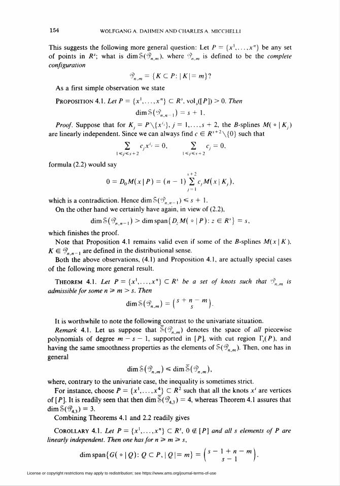
This suggests the following more general question: Let P = (x1,.. ,,x"} be any set
of points in Rs; what is dimS^ m), where 9n m is defined to be the complete
configuration
%,m={KEP:\K\=m}l
As a first simple observation we state
Proposition 4.1. Lei F = {x',...,x"} C Rs, vol5([F]) > 0. Then
dimS(^,„_,)=i+l.
Proof. Suppose that for K} = F\{x''}, j' = \,...,s + 2, the ß-splines M( o | Ay)
are linearly independent. Since we can always find c G Aî+2\{0} such that
2 Cjx'j = 0, 2 cj = 0,\<£j*Zs + 2 I«/<.y + 2
formula (2.2) would say
5 + 2
Q = D0M(x\P) = (n- 1) 2cJM{x\KJ),7=1
which is a contradiction. Hence dimSC^ n_x) < s + 1.
On the other hand we certainly have again, in view of (2.2),
dimS^ „_,) > dim span {D.M( °\P):z G Rs) = s,
which finishes the proof.
Note that Proposition 4.1 remains valid even if some of the ß-splines M(x | A),
K E.^ , are defined in the distributional sense.
Both the above observations, (4.1) and Proposition 4.1, are actually special cases
of the following more general result.
Theorem 4.1. Let P={jt',...,x")Cff be a set of knots such that 9 is
admissible for some n > m> s. Then
d.ms(úp,j = (5+rw)-
It is worthwhile to note the following contrast to the univariate situation.
Remark 4.1. Let us suppose that ?>(%„,) denotes the space of all piecewise
polynomials of degree m — s — 1, supported in [P], with cut region TS(P), and
having the same smoothness properties as the elements of §CiPn m). Then, one has in
general
dimS(^,m)<dimS(t,m),
where, contrary to the univariate case, the inequality is sometimes strict.
For instance, choose P = (x1,... ,x4} C A2 such that all the knots x' are vertices
of [P]. It is readily seen that then dim S(94 3 ) = 4, whereas Theorem 4.1 assures that
dimS(<3,43) = 3.
Combining Theorems 4.1 and 2.2 readily gives
Corollary 4.1. Let P = (x1,... ,x"} C Ä1, 0 Í [P] and all s elements of P are
linearly independent. Then one has for n > m> s,
dimspan(G(° |ô): QCP,\Q\=m) = ¡s ~ ] +_n~m\
License or copyright restrictions may apply to redistribution; see https://www.ams.org/journal-terms-of-use

linear independence of multivariate S-SPLINES. II 155
As a first basic ingredient of the proof of Theorem 4.1 we state the following
result.
Lemma 4.1. For s < m < n, P = {x',...,x"} C Rs one has
dimS(í?„ „,) = dim span \J (\ + x ■ xJ): I E {\,.. .,n) ,\I\= n - m\.Se/ '
Proof. For any finite collection G of knot sets A C Rs, (2.9) provides the following
equality:/-OO . ,
2 cKA(tx\K)= 2 cKj e-hh"-s-]M(th-xx\K)dhKe.e Kee °
= t»-' re-'hhn-s-x( 2 cKM(h-xx\K))dh,
which holds for any x G A5, t > 0. Hence from the properties of the Laplace
transform we infer that
(4.2) M( ° | A), A G G, are linearly independent if and only if
A(o |A), AGß, are.
But, referring again to the properties of the (multivariate) Laplace transform, (2.14)
implies that A( o | K), A G G, are linearly independent if and only if the rational
functions
II (1 +x-u)"', AG6,
are. In the special case when K G 6 = %m this in turn is equivalent to saying that
the polynomials
no + wx), KE%<m,u&K
are linearly independent if and only if the functions A( ° | A), A G 6Sn , and, on
account of (4.2), the ß-splines M( ° | A), A G % m are linearly independent.
Obviously, the linear space n = span(nueA-(l + u-x): A G <?Pn m) satisfies
ncn„.v
Since
dnnlin_m,s=("-m + s),
the validity of Theorem 4.1 is tantamount to showing n = UH_ms. When P
contains n — m + s points in general position, Lemma 3.1 does confirm that
n = n„_mi. In the general case this equality still holds. One approach to proving
this is to extend Lemma 3.1 to its "Hermite Form". Rather than taking this
approach we will make use of (3.2). Thus if q,(x) is any homogeneous polynomial of
degree Kn — m, there are constants p, such that
|/|=/ JEI
Therefore we also have Iln_m s C II. This proves Theorem 4.1 as well as
Proposition 4.2. Let % m be any admissible complete configuration. Then
License or copyright restrictions may apply to redistribution; see https://www.ams.org/journal-terms-of-use

156 WOLFGANG A. DAHMEN AND CHARLES A MICCHELLI
In the remaining part of this section we will be concerned primarily with methods
for generating a basis of ß-splines for the space o>(9„ „,). At the same time though,
we will introduce several useful notions applicable to arbitrary collections of knot
sets G. These ideas are motivated by two obvious facts about the univariate space
SCiT ). Although this space contains all ß-splines of degree k, it is well known that
the consecutive ß-splines corresponding to A, = {r,,... ,ti+k + x), i: = 1,... ,n — k —
1, span 5(5"). In this case the linear independence of the ß-splines M( ° |A,),
/' = l,...,n — k — 1, over [/,, tn] easily follows from the fact that each A, contains a
knot which is not in any of the previous sets A,,..., A,_,. It is important to keep in
mind that this fact is dependent on the order in which these sets are enumerated.
To place these facts in a general context we introduce the following notion
Definition 4.1. Let G be a collection of knot sets in Rs. We will say A,,..., KN G G
form a strong chain of length N provided that for each i, 1 < i < N, there is some
p G TS(K¡+X) and a point x in the relative interior of [HpC\ Kl+X] which is not in
Uw</U {yers(Kj)}.
Lemma 4.2. Let (A,, A2,..., A^) be a strong chain. Then the B-splines M( ° | A,),
i = 1,... ,yV, are linearly independent over Ul^iSiN[Kj].
Proof. M( ° | A,) is trivially linearly independent. Suppose M( ° \K¡), i = I,...,
j' — 1, are also for some/ < N. In view of the hypothesis we can find p G Ts( A ) and
a point z in the relative interior of [Hp D K-] such that z does not belong to
U|s./<7 U {y G IS(K,)}. Suppose Hp is w?-fold, i.e. Hp contains exactly s — 1 + m
knots of Kj. Defining for A J- Hp
LH(f)= lim {(Dxy-s-mf(z + tX) - (Dx)"-s-mf(z - tX)),
Proposition 2.1 assures
LHp(M(°|A,))*0.
So 2/=, c,M( ° | A,) = 0 would imply
2 c,L„(M( ° | A,)) = 0 = CjLHp{M( o\Kj)),i=\
and hence c = 0. Thus 2i<,«;y-i c,M( ° \ K¡) = 0, which by assumption means
c, = 0, i = \,...,j.
Note that in the univariate case the sequence of consecutive knot sets is obviously
the longest strong chain in 5".
This gives rise to the following
Definition 4.2. A subset % of a given knot configuration G is called an s-basis of G if
there is a chain ( A,,..., A^, ) so that
S= {A,:/= 1,...,/V=|®|),
and whenever (K[,... ,K'N,) is another chain in G then
N'<\&\.
| <3d |=F((2) is called the s-index of G and (A(: i= 1,...,|®|} is called an
s-generating sequence for G.
Example 4.1. In the univariate case the consecutive knot sets form a 1-generating
sequence for %k+2 and Ix(%ik+2) = n - k - 1.
License or copyright restrictions may apply to redistribution; see https://www.ams.org/journal-terms-of-use

LINEAR INDEPENDENCE OF MULTIVARIATE B-SPLINES. II 157
Theorem 4.2. Let « 3= m> s, P = {x\... ,x"} E Rs. Suppose P contains n — m +
s points in general position. Then
Proof. We can easily obtain an upper bound on the s-index of 9n m by combining
Lemma 4.2 and Theorem 4.1 to conclude that
IÁ%J<(S + ns~m)-
On the other hand the proof of Lemma 3.1 (cf. Lemma 2 in [7]) suggests the
following s-generating sequence for 9n m. Let Q E P denote any fixed subset
consisting of n — m + s points in general position. Then V = P\Q clearly satisfies
| K|= n — n + m — s = m — s > 0.
Now there are exactly ("~™+s) distinct subsets
i r- n ; — i I s + n — m\ , T ,I,EQ, i-\,...,\ s j, |/|=5.
Consequently, the ("~f+i) sets A, = VU I, form a strong chain in 9„ m since
I K¡■ I= I ^ I +1 h■ I ~ m holds by construction. Hence Definition 4.2 says that
1(9 )>(n~m + s)
which completes the proof.
Note that the 5-basis constructed in the above proof forms an ^-generating
sequence for 9n m even for an arbitrary ordering of the sets A,. However, in general,
the ordering will matter as is shown by the consecutive knot sets in Example 4.1.
So, when dealing with complete configurations the dimension of the correspond-
ing j-variate span of ß-splines coincides with the s-index of the configuration.
However, this simple rule is unfortunately not valid for any configuration of knot
sets even in one dimension. This is confirmed by the following
Example 4.2. Suppose xx, x2,... ,x6 are pairwise distinct univariate knots arranged
in increasing order. Let G = {A,, A2, A3, A4} where
A, = {x,,x2,x4}, A2 = (x,,x3,x5},
^3 ~~ lX4> X$, X6j, A4 — (x2, X3, X6) .
It is then easy to see that the dimension of the §>(ß) will depend on the position of
the knots.
Two important remarks concerning Lemma 4.2 and Theorem 4.2 should be made.
The first remark concerns the definition of a strong chain. This notion, being based
on the smoothness properties of the multivariate ß-spline, can be weakened while
still insuring the validity of Lemma 4.2. We only need to require that for each i,
1 < /' < N, there is some p G rj(A/+1) which is r-fold, i.e. Hp contains exactly
s + r — 1 points in K,+ x, such that either p (¿ U1<y<( U (y G Is(Kj)} or, if p E
U {y G Is(Kj)) for somey «£ /', then p is at most (r — l)-fold relative to Kj. Thus,
even though p may be contained in each U {y G Is(Kj)}, 1 =£;'<(, there is at least
one point in Hp at which the ß-spline M( ° | AI+,) has a different smoothness than
any of the ß-splines M( ° | Kj),j < i. When A,,..., A^ have this weaker property we
License or copyright restrictions may apply to redistribution; see https://www.ams.org/journal-terms-of-use

158 WOLFGANG A. DAHMEN AND CHARLES A MICCHELLI
will say (KX,...,KN) forms a weak chain. The same argument used in Lemma 4.2
guarantees that M( ° | K¡), i = 1,...,tV, are linearly independent if (KX,...,KN)
forms only a weak chain.
Finally, we wish to point out that Theorem 4.2 gives a purely combinatorial
criterion for the linear independence of ß-splines. To emphasize this point let us
observe that Definition 4.2 and Theorem 4.2 can be rephrased entirely as a
combinatorial fact.
Let P be any finite set of n objects and (P)„, the collection of all subsets of P
consisting of m objects. Thus, while (P)m is for m < n the analog of the complete
configuration of knot sets 9n m considered before, (A)J corresponds for A G (P)m,
s < m, to the cut regions IS(K), A G 9n „,. For any collection G of sets of objects we
say (KX,...,KN) is a chain of length N in G if A, G G, i = 1,...,7V, and
(4-3) (*,+i),\ U (tf,-),*0' i=h...,N-l.l«y<i
As before the i-index IS(G) is the longest chain in G.
Then it follows that for s < m < | P \
/.((n.) = (|p|-m+*),
because we can always identify P with a set of n vectors in Rs which are in general
position and (K)s with the cut region of M( ° | A). Since then every chain in the
sense of (4.3) gives rise to a strong chain of the same length in the sense of
Definition 4.1, this identification preserves the notion of chain and index so that
Theorem 4.2 is applicable.
Conversely, any collection of knot sets in Rs, each of which is in general position,
can be identified with a combinatorial structure. For instance, consider
Example 4.3. Let P = {1,2,...,6}. One may check that {{1,2,3,4}, {1,2,3,5},
{1,2,3,6}, {1,2,4,5}, {1,2,4,6}, {1,2,5,6}} form a 2-generating sequence for (F)4
and/2((F)4) = 6, whereas,/,(( F )4) = 3 because {{1,2,3,4}, {2,3,4,5}, {3,4,5,6}}
is a 1-generating sequence. Thus, if we think of F as a set of 2-vectors (four among
them being in general position, say), we have a way of obtaining six linearly
independent ß-splines spanning S(%4) while, if F is thought of as a set of
univariate knots (at least three being pairwise distinct) we obtain three independent
ß-splines.
5. Regular Configurations. We have seen in the previous section that the dimen-
sion of the linear span of ß-splines on the complete configuration is determined by
its combinatorial structure. But, unfortunately, according to Example 4.2 this is not
generally true. Nevertheless, as we shall point out next, there is another large class of
configurations which has this property and is also suitable for approximation. For
this purpose we will call a configuration G of knot sets regular if dim S(6) = 7,(6).
We will continue using the notions s-index, s-generating sequence, s-basis, chain in
both contexts, i.e. when dealing with the purely combinatorial properties of collec-
tions of sets of arbitrary objects as well as when identifying these objects with knots
in Rs and referring to the corresponding cut regions. The proper interpretation will
always be clear from the context. In particular, the analogy between both concepts
suggests calling the elements of (K)s (abstract) (s — l)-simplices.
License or copyright restrictions may apply to redistribution; see https://www.ams.org/journal-terms-of-use

LINEAR INDEPENDENCE OF MULTIVARIATE ß-SPLINES. II 159
Let us consider the following definitions taken from [9]. For any s, k G Z+ and
n = s + k let
(5.1) A(s,k)= {a= {(j„m,):i = 0,...,n}:jn = mn = 0,
U,mr)<(jr+X,mr+X),(jr,mr) E {0,...,s} X{0,...,*}}.
Note that
(5.2) \A(s,k)\=[s + k), (jn,m„) = (s,k).
For 7 = {i0,... ,is) G Z\ we define
A(I,k) = {{(ijr,mr):r = 0,...,«}: {(¿, *,): r = 0,...,«} £A(a)}.
There is a simple geometrical interpretation of A(s, k). Let p = [u°,...,us], y —
[v°.vk] be simplices in Rs, Rk, respectively. Then
(5.3) %<y= [oK = [(«>•, t>"">),..., (uJ-,vm-)]:
K= {(Jr,mr):r = 0,...,n) E-A(s,k)}
is a triangulation of pXyC A". Here a collection 9" of simplices is called a
triangulation of ß when ß = U{o£Î) and the intersection of any two elements of
"T is empty or a common lower-dimensional face.
Now suppose $ E Z++ ' induces an (abstract) simplicial s-complex, i.e. j- is
combinatorially equivalent to a triangulation UJ of some polyhedral domain Q in Av,
which means that there is a one-to-one inclusion preserving correspondence between
the sets of all faces of the elements of % and bJ, respectively. The configuration
(5.4) A(M)= U {A(I,k):lE^}
is known to form an (abstract) simplicial «-complex (cf. [8], [9, Lemma 8.9]).
In particular, when CV= {u': i — 1,... ,7V} C AJ are chosen so that
(5.5) 0(^)={p(7)=[M'o,...,M'.]:7={/o,...,/J}G^}
is a triangulation of ß = U {p(7): 7 G f}, the collection
(5.6) %= {l{ui<o,em°),...,(uiJ*,em")]: {(iJr, m,): r = 0,...,«} EA(},t))
is a triangulation of Í2 X Ss, Sk = [e°,...,ek], (eJ), = «,._,, i, j = 0,...,k (cf. [8],
[13]).Before explaining the connection with certain spline spaces we state
Theorem 5.1. Let A(f, k) be defined by (5.4). Then one has
Is(A(j,k))=\A(f,k)\,
i.e. A(j-, k) forms an s-basis (cf. Definition 4.1, (4.3)).
Proof. We have to show that the elements of A(f, k) can be ordered in such a way
that condition (4.3) is satisfied. To this end, we shall show first that the assertion is
true for k = 0.
Lemma 5.1. Let $ E Z++ ' induce a simplicial s-complex. Then
License or copyright restrictions may apply to redistribution; see https://www.ams.org/journal-terms-of-use

160 WOLFGANG A. DAHMEN AND CHARLES A. MICCHELLI
Proof. Suppose \%\~ m. Without loss of generality we may assume that J is a
triangulation of some bounded polyhedral domain ß in Rs. Hence one can find an
element of j such that at least one of its (s — l)-faces is contained in the boundary
of ñ and is therefore not shared by any other element of J. Choose Im to be such an
external element. Next let Im_x be any external element of f\{Im), etc. Clearly
{7,,..., Im} form a chain.
So, suppose f = {I¡: i = 1.| ¡| |} is a chain so that there are (s — l)-simplices
P,E(/,)„ p,G U (/,),.i«y</
In order to finish the proof of Theorem 5.1, we only have to show now in view of
(5.4) that the elements of each A(7,, k) can be ordered as
A(7,,*)={a,,:;=1,...,(* + *)},
say, so that there is p] G (A, )f, p7 G U,^r<-(K,. r)s, and the first components of the
pairs in py coincide exactly with the elements of p, G ( I, )s above.
The existence of such an ordering for A(7,, k) is affirmed by the following
Lemma 5.2. For any s, k G Z+ and any fixed i G {0,... ,s) there is an ordering
{K/.] = \,...,(5 + k)}forA(s, k)(5.\)such that there is
(5.7) Pj={(Jr,mr):r=0,...,s,jr^i}E(KJ)s, Pj £ IJ (*,),.l</</-l
Proof. The cases s, k — 0 are trivial. Let us first prove the assertion for s — 1,
k G TV. For / = 1 the ordering
Kj={(0,0),...,(0,j),(l,j),...,(l,k)}, j = 0,...,k,
obviously works, whereas for i = 0 the reverse ordering will do.
So, we may assume that we have proved the assertion for s — 1 > 1 and all
k G Z+ . For the purpose of advancing the induction step, we introduce the
following subsets of A(s, k).
Cm = {A G A(s, k): (jn_r, mn_r) = (s,k~ r),
r = 0,... ,m, j, < s, i < n — m), m — 0,... ,k.
By definition (5.1) and (5.2) one has therefore
(5.8) AGC„, iffA= A' U {(s, k- m),..., (s,k)), K' G A(s - 1, k - m),
and hence again by (5.2)
i n i — i Kt i ; w— ( s — \ + k — m\\Cm\-\A(s- \,k- m)\- ( s_ j j.
Since obviously C, flC= 0, / i=j, and
m = 0 m — KJ
we conclude
k
A(s,k)= U Cm.m=0
License or copyright restrictions may apply to redistribution; see https://www.ams.org/journal-terms-of-use

LINEAR INDEPENDENCE OF MULTIVARIATE S-SPLINES. II 161
Suppose now i =£ s. By assumption there exists for each m = 0,... ,k an ordering
(A7:y=l.(s-\+_\-m)}=A(s-l,k-m),
such that
P™ = {U. mr):r = 0,...,s - 1, jr* i) G (*/),_,,
but
p;g u (*;),_,.I«<7«/-1
So, defining
*; u {(,,*)}; y=i.-.('7lt*).
'•" y=^.<)-('7lt*) + - + (-1+,*_7- + ')+'-w = 1,... ,/c,
the corresponding sequence of (5 — l)-simplices
p; = p"' U {(5, & - m)} when/' =j(m, i)
obviously satisfies (5.7) since (s, k — m) never occurs in a preceding block.
Now suppose /' = s. Associating with each
A= {(jr,mr):r = 0,...,n} EA(s,k)
the set
K= {(\jr-s\ ,\mr- k\):r = 0,...,n}
defines evidently a bijective map from A(s, k) onto itself where /' = s is mapped into
/' = 0. So the sets A may be ordered now by the same procedure as before, thereby
inducing an appropriate ordering for the original sets A as well. This finishes the
proof of Lemma 5.2.
Recalling our remarks subsequent to Lemma 5.1, the construction of an s-generat-
ing sequence for A(f, k) with length | A(f, k) | is now an immediate consequence of
Lemmas 5.1, 5.2, which completes the proof of Theorem 5.1.
As to the connection with certain spline spaces let again
<V= {ui-J;i= l,...,N,j = 0,...,k}
be a collection of points in R5 such that for some $ E Zs+ '
(5.9) ®($) = {p(I)=[u^,...,u--°]:I={tn,...,is}Ef}
is a triangulation of ß = U {p(7): 7 G f}.
Defining now for A = {(/., mr): r = 0,...,n} G A(j-, k) the knot set
(5.10) C(A)= {uJ"'m«,...,uJ-m"},
it was shown in [6], [8], [13] that the collection {M( ° | C(A)): A G A(f, k)}, forms
a basis for S(6), G = {C(A): A G A(f, k)}, provided the knots u'J are sufficiently
License or copyright restrictions may apply to redistribution; see https://www.ams.org/journal-terms-of-use

162 WOLFGANG A. DAHMEN AND CHARLES A. MICCHELLI
close to u'-° for all ;, /'. Moreover, under these assumptions the above basis turns out
to be very well conditioned. This type of a basis is of particular interest because the
corresponding spline spaces exhibit very good approximation properties (cf. [6], [8],
[13]).However, one may expect that the above type of restrictions on the knot positions
is not essential for the linear independence of the ß-splines M( ° | C), C G G. In
fact, Theorem 5.1 allows us to formulate sufficient conditions for their linear
independence which do not involve distances between knots and instead are satisfied
for 'almost all' knot positions.
To this end let us call any configuration of knot sets in Rs nondegenerate if there
exists an s-generating sequence in the sense of (4.3) which at the same time forms a
weak chain. Then, recalling the remarks subsequent to Example 4.2, we may
rephrase Theorem 5.1 as
Corollary 5.1. Let G be defined as above with respect to a set of knots £V= [u'-J]
in Rs. If G is nondegenerate, then {M( ° \ C): C G G] forms a basis for %(Q), i.e. 6 is
regular and
dimS(e) =\e\=is(e).
The simplest concrete condition to ensure nondegeneracy of G is, of course, to
require that T is in general position. But nondegeneracy certainly holds under
weaker assumptions. For instance if
(i) the collections {(C(A,-,): j = 1,... ,(s+sk))} (cf. (5.10)), A,,, G A(7„ k), j =
\,...,(s+sk), are weak chains in G for 1 < /' <| \\ and if
(ii) vols_,(p n p') = 0 whenever p G C(A), p' G (A'), A n A' = 0, A, A' G
A(f,k),then G is nondegenerate since the chain constructed in the proof of Theorem 5.1 by
composing the 'local chains' in A(7,, k) (cf. Lemma 5.2) induces a weak chain of the
same length in G.
Condition (i) in turn holds if for instance all A G G are individually in general
position or if each element of 0(f) (cf. (5.9)) forms a proper i-simplex and the sets
{ujn':j El,m = 0,...,k}
are for each 7 G \ in general position.
The authors believe that the above assertion is even valid in a more general sense,
namely when the configuration G is induced by any triangulation (cf. (5.6), (5.9)) of
A* X A* with the property that all the vertices of the corresponding (s + fc)-simplices
belong to U {Rs X {e'}: i = 0,... ,k}. This latter condition is known to be neces-
sary [6]. Moreover, when Sk is replaced by any &-polytope with more than k + 1
vertices, the induced collection of ß-splines is always linearly dependent [6]. Hence
one has in this case, even if the corresponding configuration G is nondegenerate,
i,(e)<\e
License or copyright restrictions may apply to redistribution; see https://www.ams.org/journal-terms-of-use

LINEAR INDEPENDENCE OF MULTIVARIATE ß-SPLINES. II 163
Acknowledgement. The authors would like to thank the referee for his valuable
suggestions and comments, in particular, simplifying the proof of Lemma 5.1.
The principal results of this paper were obtained during the winter of 1979 while
the first author was an IBM Postdoctoral Fellow at the Thomas J. Watson Research
Center.
Fakultät für Mathematik
Universität Bielefeld
Universitätsstrasse
48 Bielefeld, West Germany
IBM Thomas J. Watson Research Center
P. O. Box 218
Yorktown Heights, New York 10598
1. C. de Boor, "Splines as linear combinations of ß-splines," Approximation Theory II (G. G. Lorentz,
C. K. Chui, L. L. Schumaker, Eds.), Academic Press> New York, 1976, pp. 1-47.
2. A. S. Cavaretta, C. A. Micchelli & A. Sharma, "Multivariate interpolation and the Radon
transform," Math. Z., v. 174, 1980, pp. 263-279.
3. K. C. Chung & T. H. Yao, "On lattices admitting unique Lagrange interpolations," SIAM J.
Numer. Anal., v. 14, 1977, pp. 735-743.
4. H. B. Curry & I. J. Schoenberg, "On Pólya frequency functions IV. The fundamental spline
functions and their limits," /. Analyse Math., v. 17, 1966, pp. 71-107.
5. W. Dahmen, "On multivariate ß-splines," SIAMJ. Numer. Anal., v. 17, 1980, pp. 179-191.
6. W. Dahmen, Multivariate B-Splines—ein neuer Ansatz im Rahmen der konstruktiven mehrdi-
mensionalen Approximationstheorie, Habilitationsschrift, Bonn, 1981.
7. W. Dahmen & C. A. Micchelli, "On the limits of multivariate ß-splines," /. Analyse Math., v. 39,
1981, pp. 256-278.
8. W. Dahmen & C. A. Micchelli, "On the linear independence of multivariate ß-splines. I:
Triangulations of simploids," SIAM J. Numer. Anal., v. 19, 1982, pp. 993-1012.
9. S. Eilenberg & N. Steenrod, Foundations of Algebraic Topology, Princeton Univ. Press, Princeton,
N. J., 1952.
10. I. M. Gel'fand, M. I. Graev & N. Y. Vilenkin, Generalized Functions V, Academic Press, New
York, 1966.
H.H. Hakopian, "Multivariate spline functions, ß-spline basis and polynomial interpolations," SIAM
J. Numer. Anal., v. 19, 1982, pp. 510-517.
12. H. Hakopian, "Les différences divisées de plusieurs variables et les interpolations multidimension-
nelles de types Lagrangien et Hermitien," C. R. Acad. Sei. Paris, v. 292, 1981, pp. 453-456.
13. K. HÖLLIG, "Multivariate splines," SIAM J. Numer. Anal., v. 19, 1982, pp. 1013-1031.
14. C. A. Micchelli, "A constructive approach to Kergin interpolation in Rk: Multivariate ß-splines
and Lagrange interpolation," Rocky Mountain J. Math., v. 10, 1980, pp. 485-497.
15. C. A. Micchelli, "On a numerically efficient method for computing multivariate ß-splines,"
Multivariate Approximation Theory (W. Schempp, K. Zeller, Eds.), Birkhauser, Basel, 1979, pp. 211-248.
License or copyright restrictions may apply to redistribution; see https://www.ams.org/journal-terms-of-use