On the Inverse Filtering of Speech - University of Cretekafentz/Thesis_Final.pdf · On the Inverse...
98
University of Crete FO.R.T.H. Department of Computer Science Institute of Computer Science On the Inverse Filtering of Speech (MSc. Thesis) George P. Kafentzis Heraklion October 2010
-
Upload
truongtruc -
Category
Documents
-
view
215 -
download
0
Transcript of On the Inverse Filtering of Speech - University of Cretekafentz/Thesis_Final.pdf · On the Inverse...

University of Crete FO.R.T.H.Department of Computer Science Institute of Computer Science
On the Inverse Filtering of Speech
(MSc. Thesis)
George P. Kafentzis
Heraklion
October 2010

Department of Computer Science
University of Crete
On the Inverse Filtering of Speech
Submitted to the
Department of Computer Science
in partial fulfillment of the requirements for the degree of
Master of Science
October 22, 2010
c© 2010 University of Crete & ICS-FO.R.T.H. All rights reserved.
Author:George P. Kafentzis
Department of Computer Science
Committee
SupervisorYannis Stylianou
Associate Professor
MemberAthanasios MouchtarisAssistant Professor
MemberPanagiotis Tsakalides
Professor
Accepted by:
Chairman of theGraduate Studies Committee Panos Trahanias
Professor
Heraklion, October 2010


ON THE INVERSE FILTERING OF SPEECH
by
George P. Kafentzis
A thesis submitted to the faculty of
University Of Crete
in partial fulfillment of the requirements for the degree of
Master of Science
Computer Science Department
University of Crete
September 2010

Copyright c© 2010 George P. Kafentzis
All Rights Reserved
ABSTRACT
ON THE INVERSE FILTERING OF SPEECH
George P. Kafentzis
Computer Science Department
Master of Science
In all proposed source-filter models of speech production, Inverse Filtering
(IF) is a well known technique for obtaining the glottal flow waveform, which
acts as the source in the vocal tract system. The estimation of glottal flow is
of high interest in a variety of speech areas, such as voice quality assessment,
speech coding and synthesis as well as speech modifications. A major obstacle
in comparing and/or suggesting improvements in the current state of the art
approaches is simply the lack of real data concerning the glottal flow. In other
words, the results obtained from various inverse filtering algorithms, cannot
be directly evaluated because the actual glottal flow waveform is simply un-
known. To this direction, suggestions on the use of synthetic speech that has
been created using artificial glottal waveform are widely used in the literature.
This kind of evaluation, however, is not truly objective because speech synthe-
sis and IF are typically based on similar models of the human voice production
apparatus, in our case, the traditional source-filter model. This thesis presents
three well-known IF methods based on Linear Prediction Analysis (LPA), and
a new method, and its performance is compared to the others. The first one
is based on the conventional autocorrelation LPA, and the second one on the
conventional closed phase covariance LPA. The closed phase is identified using
Plumpe and Quatieri’s suggested method based on using statistics on the first
formant frequencies during a pitch period. The third one is based the work
of Alku et al, which proposed an IF method based on a Mathematically Con-
strained Closed Phase Covariance LPA, in which mathematical constraints are
imposed on the conventional covariance analysis. This results in more realis-
tic root locations of the model on the z-plane. Finally, Magi et al suggested a
new method for extracting the vocal tract filter, called Stabilized Weighted LP
Analysis (SWLP), in which a short time energy window controls the perfor-
mance of the LP model. This method is suggested for IF due to its interesting
property of applying emphasis on speech samples which typically occur during
the closed phase region of the speech signal. This is expected to yield a more
robust, in the acoustic sense, vocal tract filter estimate than the conventional
autocorrelation LP. The three IF approaches along with the suggested new
one are applied on a database of physically modeled speech signals. In this
case, the glottal flow and the speech signal are available and direct evaluation
of IF methods can be performed. Robust time and frequency parametrization
measures are applied on both the actual glottal flow and the estimated ones,
in order to evaluate the performance of the methods. These measures include
the Normalized Amplitude Quotient (NAQ), the difference between the first
two harmonics (H1-H2) of the glottal spectrum, and the Harmonic Richness
Factor (HRF), along with the Signal to Reconstruction Error ratio (SRER).

Experiments conducted on physically modeled sustained vowels (/aa/, /ae/,
/eh/, /ih/) of a wide range of frequencies (105 to 255 Hz) for both male and
female speech. Glottal flow estimates were produced, using short time pitch
synchronous analysis and synthesis for the covariance based methods, whereas
for the autocorrelation methods, a long analysis window and a short synthe-
sis window was used. The results and measures are compared and discussed,
showing the prevalence of the covariance methods, but the suggested method
typically produces better results than the conventional autocorrelation LP,
according to our metrics.

vi

ACKNOWLEDGMENTS
First, I would like to thank my supervisor, Professor Yannis Stylianou,
for his continuous support in the M.Sc. program. I am really grateful for
his advice, encouragement, guidance, motivation, and above all, trust and
patience that he showed during the time we worked together. He gave me
the chance to meet and work with exceptional people and scientists. He also
taught me how to view things from different perspectives, how to do research,
and how to be persistent when things are not going well. Finally, his help and
care on matters beyond academia were really emotive, and for this I thank
him twice.
I also thank Professor Paavo Alku, whom I had the opportunity to meet and
work with in the Acoustics and Signal Processing Laboratory of the Aalto Uni-
versity of Technology, Helsinki, Finland, for his hospitality, kindness, support,
and guidance, and for providing me the physically modeled speech database
to work with in this Thesis.
In addition, I would like to thank Dr. Olivier Rosec, whom I had the
opportunity to work with for four months in France Telecom R & D, Lannion,
France. His continuous support during my stay there was very important for
me.
I also thank my colleagues, past and present, with whom I shared my
days at the University of Crete, and especially in the Multimedia Informatics
Laboratory of the Computer Science Department. They made it a wonder-

viii
ful workplace and home for the past years. I would like to specially mention
Christos and George Tzagkarakis, Pavlos Mattheakis, Maria Koutsogiannaki,
Mairi Astrinaki, George Tzedakis, George Grekas, Christina Lionoudaki, Yan-
nis Agiomyrgiannakis, Miltos Vasilakis, Yannis Pantazis, Andre Holzapfel,
Maria Markaki, Nikos Pappas, Ilias Tsompanidis, Evgenios Kornaropoulos,
and Dimitris Milioris, for helping me in so many ways and for being real
friends.
Moreover, I would like to say ”thank you” to many others, including George
Charitos, Kostas Perakakis, George Charitonidis, Pepi Katsigianni, Petros An-
drovitsaneas, Kostas Sipsas, Nasos Lagios, Andreas Vourdoulas, Panayotis
Tripolitis, Eleni Choremioti, and Kostas Katsaros, for their care and friend-
ship, even if most of them are away from Crete.
I am also grateful to the Institute of Computer Science (ICS) of the Foun-
dation of Research and Technology - Hellas (F.O.R.T.H), for awarding me a
fellowship during my graduate studies.
Last, but not least, I thank my family: my parents, Panayotis Kafentzis
and Diamanto Tsirolia, for everything. I owe them the man I am today. My
little sister Maria-Chrysanthi, for her patience, love, care, and support, in all
these years we are together in Crete. My little brother Stelios, for his love and
care, and for listening to his voice almost every night before going to bed.


ix
��������
�� ��� �� ���������� ��� �� ����� � ������ ��� ��������� ������ � ���
������ ��������� ���� ���� �� ������ ������ �� ��� �������� ��� ��������
��� ��� ����� ��� ���� �� �������� �� ���� �� �!����� ��� �������� !"
# �������� ��� ����� ��� ��� ���� �$��! �� �� ���� �� �� ���!���� �� ��
��� ��� ��� ������ ���� ��� ����� ��� ������� ������ � �� ������ ��
� �!�%��� ������ ��%&� ������ �� � �������� �����" '(�� ����� ���� ���
�!����� ��)� ���� ������� *���&���� ��� ���� �� ��������� ��%� �� ����
� ���$� ��������&� � � ��� �� ���!� �� ����� �� ��" +� ���� �����
����&����� �������� � ����� ��� ��� ��� ����� �����%��� ��� ��
���!� �� �,���%!� ���������� ���� �� �� � ��������� ��������� �����
� ��� ��� ���� �������" -�� ����� ��� ����!%����� ������!��� ���%��� �
�������� � ����� �� ��� ������%�� �� ���%��� � �������� � ����� ���
���" '.���� ���! �� �!�� � �,������ �� ���� ��������� ���������� ����
� � �!�%��� ����� �� �� *���/��� �� � ��� � ��� ��������� ��%�&����
������ ��" � ������ ��� � ����� � ������" �� ���� �� ���*� ������/���
���� ����� � � % �� *���� ��� �� ��� � ��� 0������� -��*��$�� �0-�
�� �� � � � % � ��� ���� � ��� �� �� ����� �� �� �� �� �� �������" #
��&�� *���/��� ���� ������ ������� 0- �� �� � % ��� ������� ���� �� �
�!���� ���� ������ ������� 0- ���� ������ ���� ��� ������ �� �� �� � %
��� ��� ������" # ������ ���� ������� �� ��� ���������� ��� ��� Quati-
er �� Plumpe � % �� *���/��� �� ������� � ��&��� ��,�� ���� ���� ������
��� ���������� �� ��&�� ������ �� �� ���� " (������ ���� ������� �� Alku�
����%��� �� � % � �� �� *���/��� ���� ������� 0- �� �� � % ��� ��� ���
���� �� ������ ���� �� +�%�����!� -�����!�� ��� ���� ������ ������� 0-
��� ������ ������/��� ��%������ ������� �� ������!� �� � ������� �

x
% ��� ��� �/&� �� ��� �� �� ��� �� ����� " 1 ��� ���� ������� �� Magi�
����%��� � (����%�� ������� 0- �� 2��� �Stabilised Weighted Linear Prediction��
���� ��� �� ����%�� �� ����� ����� ������ ������ �� ��� ��� ��� ��
�� ��� �� 0-" -�������� �� ����� ��� �� �� ���� ��� ������� �����
��� ���� ��� �� ������ ���� ������ ���� ��� ������ ��� � ��� ���� ���� ��
���� �� �������� �� ������ ��� �������� ! �� ���� � ����� �� ��� ���
����� ���� �� ��������� ����� ��� �������� !" ���� � ������� ��/�
�� �� � ����� � �� ��� ������� 0- �� �� � % ��� ��� ������ �� ��%��
����!� ������!�� ������������ �� �� *��� � � ��� ��� ������ ����� ��
��� �����%�� ��� ����� ���������� �� ��������� ��������� �����" ��
����� ��� ���������� � ����� �� �� �� � ���� ����� ���� �% ��� �� �����
�� ���������%�� ���������� �,������ ��� ��%� �� ��" (!������ ����� �
�������������� �������%���� ��� �� �� � �� ����� �� �� �� ����
��� ����������� �� �� �����%�� � ������ ��� ��������&� ������� �� ��� �
�� �����%���� ��� �� ��%� �� ��" ��� � ����� � ������*���� �� 3����
���� � 4�� -����� �Normalized Amplitude Quotient - NAQ�� �� ����
����,! ��� � ��&��� �����&� �� ������� ��� ����� ��� ���� H1-H2� ��
�� -������� ��%���� �����&� �Harmonic Richness Factor - HRF�� ��/� �� �
��� ������ ��� ������ ������������� �Signal to Reconstruction Error ratio -
SRER�" -������� �,��%���� �� ������ �������� �)��)� )��)� )�)� ))� ��� ���
��������%���� *��� �� �� �!�� ��������� �567 �� 877 Hz� �� �������� ���
��� �� ���� �� �� ��� ��������� �����" # ������� �� � �!�%��� ��� �����������
��������&� ����� ��� ��� ��� �!����� �� �� ���� �� �� ������ �pitch
synchronously� �� ����� ���! ����%!�� �!�%���� �� �������� �� �� ��%� ��
��� ������� �� ������ ����%��� �������� �� ���! ����%!�� �!�%���� ��
�� ��%� �� ������� ����" 1� ����� ����� ���� ���!�� ��� �� � �� ������

xi
��� ��� ��%� �� ��� ������ ���� � ���������� � % � ���� �� ��� �������
��%� � ������� ����� �!����� �� �� ����� � �� �������%����"

xii

Contents
Table of Contents xv
List of Figures xvii
1 Introduction 11.1 Background . . . . . . . . . . . . . . . . . . . . . . . . . . . . . . . . 2
1.1.1 Source-Filter Production Model . . . . . . . . . . . . . . . . . 21.1.2 Linear Prediction Analysis . . . . . . . . . . . . . . . . . . . . 31.1.3 Inverse Filtering . . . . . . . . . . . . . . . . . . . . . . . . . . 41.1.4 The Glottal Flow . . . . . . . . . . . . . . . . . . . . . . . . . 51.1.5 Closed Phase Inverse Filtering . . . . . . . . . . . . . . . . . . 71.1.6 Parametrization of the Source . . . . . . . . . . . . . . . . . . 8
1.2 Evaluation of Inverse Filtering Methods . . . . . . . . . . . . . . . . . 141.3 Physical Modeling of Speech Signals . . . . . . . . . . . . . . . . . . . 151.4 Thesis Contribution . . . . . . . . . . . . . . . . . . . . . . . . . . . . 191.5 Thesis Organization . . . . . . . . . . . . . . . . . . . . . . . . . . . . 20
2 Vocal Tract Filter Estimation with Linear Prediction 212.1 Autocorrelation based methods . . . . . . . . . . . . . . . . . . . . . 21
2.1.1 Classic Linear Prediction - Autocorrelation Method . . . . . . 212.1.2 Stabilized Weighted Linear Prediction . . . . . . . . . . . . . 23
2.2 Covariance based methods . . . . . . . . . . . . . . . . . . . . . . . . 272.2.1 Classic Linear Prediction - Covariance Method . . . . . . . . . 272.2.2 Constrained Closed Phase Covariance Linear Prediction . . . . 29
2.3 Inverse Filtering Procedure . . . . . . . . . . . . . . . . . . . . . . . . 382.3.1 VUS detector . . . . . . . . . . . . . . . . . . . . . . . . . . . 392.3.2 Pitch Estimation . . . . . . . . . . . . . . . . . . . . . . . . . 392.3.3 Excitation Instants Detection . . . . . . . . . . . . . . . . . . 392.3.4 Covariance-based LP Analysis . . . . . . . . . . . . . . . . . . 402.3.5 Autocorrelation-based LP Analysis . . . . . . . . . . . . . . . 41
2.4 Summary . . . . . . . . . . . . . . . . . . . . . . . . . . . . . . . . . 41
xv

xvi CONTENTS
3 Results 433.1 Glottal Flow Estimates Examples . . . . . . . . . . . . . . . . . . . . 433.2 Parametrization Results . . . . . . . . . . . . . . . . . . . . . . . . . 45
3.2.1 Signal to Recontruction Error Ratio - SRER . . . . . . . . . . 473.2.2 Normalized Amplitude Quotient - NAQ . . . . . . . . . . . . . 513.2.3 H1-H2 . . . . . . . . . . . . . . . . . . . . . . . . . . . . . . . 543.2.4 Harmonic Richness Factor - HRF . . . . . . . . . . . . . . . . 55
3.3 Summary . . . . . . . . . . . . . . . . . . . . . . . . . . . . . . . . . 56
4 Conclusions 594.1 Summary of Findings . . . . . . . . . . . . . . . . . . . . . . . . . . . 594.2 Suggestions for Future Work . . . . . . . . . . . . . . . . . . . . . . . 61
Bibliography 65

List of Figures
1.1 Simple Source-Filter Model . . . . . . . . . . . . . . . . . . . . . . . 21.2 Phases of the glottal flow and its derivative . . . . . . . . . . . . . . . 61.3 Liljencrants-Fant Model . . . . . . . . . . . . . . . . . . . . . . . . . 121.4 Schematic diagram of the lumped-element vocal fold model. . . . . . 161.5 Area function representation of the trachea and vocal tract . . . . . . 18
2.1 STE and Glottal Flow closed phase relation . . . . . . . . . . . . . . 262.2 Covariance Frame Misalignment and Glottal Flow Distortion . . . . . 302.3 Distortion caused by non-minimum phase filter . . . . . . . . . . . . 332.4 Examples of all-pole spectra . . . . . . . . . . . . . . . . . . . . . . . 362.5 Inverse Filtering Procedure . . . . . . . . . . . . . . . . . . . . . . . . 38
3.1 Glottal flow estimates for vowel /aa/, fundamental frequency of 105 Hz 443.2 Glottal flow estimates for vowel /aa/, fundamental frequency of 145 Hz 453.3 Glottal flow estimates for vowel /ae/, fundamental frequency of 145 Hz 463.4 Glottal flow estimates for vowel /ae/, fundamental frequency of 210 Hz 473.5 Glottal flow estimates for vowel /ih/, fundamental frequency of 115 Hz 483.6 Glottal flow estimates for vowel /ih/, fundamental frequency of 230 Hz 493.7 Glottal flow estimates for vowel /eh/, fundamental frequency of 105 Hz 503.8 Glottal flow estimates for vowel /eh/, fundamental frequency of 255 Hz 51
xvii

xviii LIST OF FIGURES

List of Tables
1.1 LF-model parameters . . . . . . . . . . . . . . . . . . . . . . . . . . . 131.2 Input parameters for the vocal fold model . . . . . . . . . . . . . . . 17
3.1 SRER mean and std, for each IF method per vowel . . . . . . . . . . 523.2 SRER mean and std for each IF method per frequency . . . . . . . . 523.3 NAQrat mean and std for each IF method per vowel . . . . . . . . . . 533.4 NAQrat mean and std for each IF method per frequency . . . . . . . 533.5 H1−H2dif mean and std for each IF method per vowel . . . . . . . 543.6 H1−H2dif mean and std for each IF method per frequency . . . . . 553.7 HRFdif mean and std for each IF method per vowel . . . . . . . . . . 563.8 HRFdif mean and std for each IF method per frequency . . . . . . . 57
xix

Chapter 1
Introduction
The source of human speech production system, called the glottal flow, poses an im-
portant role on the characteristics of speech and on several scientific fields. The glottal
flow can be obtained from the speech signal using a technique called inverse filtering
(IF). Inverse filtering is extensively used in basic research of speech production and
its applications to speech analysis, synthesis, and modification. Also, an increased
interest is recently risen in areas of speech science as environmental voice care, voice
pathology detection, and analysis of the emotional content of speech.
Most of the suggested techniques in the literature are based on Linear Prediction
(LP) Analysis [43]. The goal of this thesis is to evaluate the performance of a number
of IF techniques, using robust time and frequency domain parametrization measures
on a database of physically modeled speech signals. This chapter starts with a math-
ematical framework of the source-filter model of speech production. We then provide
motivation for the importance of assessing the performance of IF techniques and this
is followed by a description of previous efforts towards that direction. Finally, we
discuss the contribution of this thesis and we provide an outline for the remainder of
this thesis.
1

2 Chapter 1 Introduction
1.1 Background
A mathematical framework of the classic source-filter model of speech production
model is presented here.
1.1.1 Source-Filter Production Model
Speech production can be considered as a linear filtering operation, which is time
invariant over short time periods. The overall system of speech production can be
divided into three parts: the vocal tract, with impulse response v[n], the excitation
signal e[n], which is the input of the vocal tract, and the lip radiation r[n]:
s[n] = e[n] ∗ v[n] ∗ r[n]
where s[n] is the speech pressure output, i.e. the speech signal, and * denotes
convolution. For voiced speech, the excitation is a periodic series of pulses, whereas
for unvoiced speech, the excitation has the properties of random noise. Figure 1.1
depicts this simple model.
Series of impulsesor random noise
Source signal e[n]
Vocal tract signal v[n]
Lip radiation r[n]
Speech s[n]
Figure 1.1 Simple Source-Filter Model.
In the Z-domain, the above equation can be written as:
S(z) = E(z)V (z)R(z)
It is shown that the vocal tract filter V (z) can be written as an all-pole filter:
V (z) =1∏p
k=1(1− ckz−1)=
1∑pk=1(αkz−k)
,
where p is the number of poles of the filter.
1.1 Background 3
1.1.2 Linear Prediction Analysis
A primary tool for inverse filtering speech waveforms is Linear Prediction (LP). LP is
a very powerful modeling technique which may be applied to time series data. When
applied to the speech signal, LP is used to produce an all-pole model of the system
filter, V (z), which turns out to be a model of the vocal tract and its resonances or
formants. As it is previously mentioned, the input to such a model is either a series
of pulses or white noise, for voiced speech and unvoiced speech respectively.
So, using LP we can estimate the vocal tract filter v[n] from the speech signal, and
then cancel its effect, thus resulting in the source waveform. In order to find the vocal
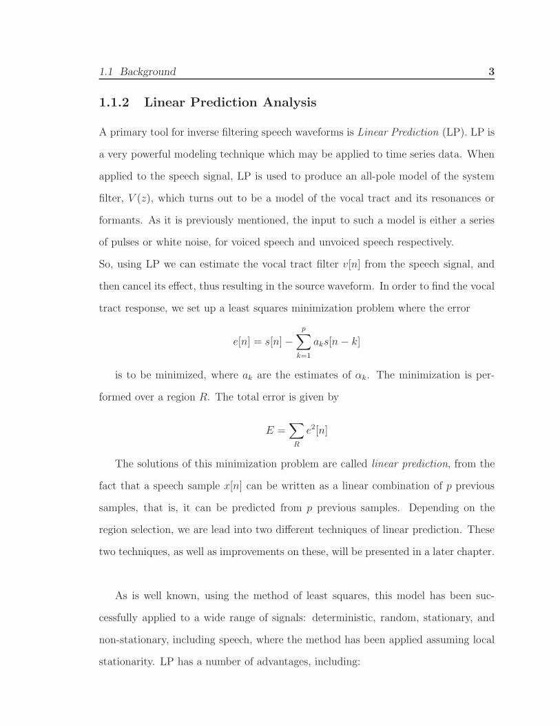
tract response, we set up a least squares minimization problem where the error
e[n] = s[n]−p∑
k=1
aks[n− k]
is to be minimized, where ak are the estimates of αk. The minimization is per-
formed over a region R. The total error is given by
E =∑R
e2[n]
The solutions of this minimization problem are called linear prediction, from the
fact that a speech sample x[n] can be written as a linear combination of p previous
samples, that is, it can be predicted from p previous samples. Depending on the
region selection, we are lead into two different techniques of linear prediction. These
two techniques, as well as improvements on these, will be presented in a later chapter.
As is well known, using the method of least squares, this model has been suc-
cessfully applied to a wide range of signals: deterministic, random, stationary, and
non-stationary, including speech, where the method has been applied assuming local
stationarity. LP has a number of advantages, including:

4 Chapter 1 Introduction
1. Mathematical tractability of the error measure
2. Stability of the model
3. Favorable computational characteristics of the resulting formulations
4. Spectral estimation properties
5. Wide applicability to a range of signal types
1.1.3 Inverse Filtering
The idea behind inverse filtering is to form a computational model for the vocal
tract signal and then to cancel its effect from the speech waveform by filtering the
speech signal through the inverse of the model. When we obtain an estimate, V (z),
of the vocal tract filter V (z), we can cancel its effect by removing the vocal tract
response from the speech signal s[n]. After that, we have an estimate of the driving
function, e[n], which is the combined signal of the glottal flow and the lip radiation.
In frequency domain,
E(z) =S(z)
V (z).
The above equation describes a process called inverse filtering. It is apparent that
inverse filtering is greatly depended on the estimate of the vocal tract filter, V (z).
The problem of robustly and accurately estimation of the vocal tract is often called
spectral estimation in the literature.
A common procedure before linear prediction analysis and inverse filtering is pre-
emphasizing the speech signal. Pre-emphasis is the process of filtering the speech
signal with a single zero high-pass filter:

1.1 Background 5
semph = s[n]− βemphs[n− 1],
where βemph is the pre-emphasis coefficient and its values are between 0.9 and 0.99.
The reason for pre-emphasis is that the pre-emphasized spectrum is a closer repre-
sentation of the vocal tract response, thus allowing linear prediction to better match
the vocal tract response rather than the spectrum of the combined excitation and
vocal tract.
Another common procedure before applying vocal tract LP analysis is applying a
LP analysis of order one to acquire a preliminary estimate for the combined effects
of the glottal flow and the lip radiation effect on the speech spectrum. Then, the es-
timated effects are cancelled from speech by invserse filtering with the corresponding
filter.
1.1.4 The Glottal Flow
The goal of inverse filtering is the estimation of the voice source, e.g. the glottal flow.
The glottal flow is the output of the glottis during voicing and thus it is a periodic
signal. A period of the glottal flow can be divided in two main parts, corresponding
to the state of the glottis:
1. The glottal open phase, where the glottis starts to open, reaches its full openess,
and eventually closes again. The open phase can be further divided into the
opening phase, where the glottal flow increases from baseline at time 0 to its
maximum amplitude Av, also called amplitude of voicing at time Tp, and the
6 Chapter 1 Introduction
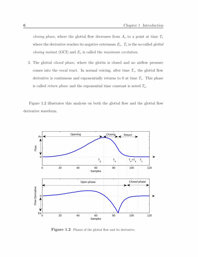
closing phase, where the glottal flow decreases from Av to a point at time Te
where the derivative reaches its negative extremum Ee. Te is the so-called glottal
closing instant (GCI) and Ee is called the maximum excitation.
2. The glottal closed phase, where the glottis is closed and no airflow pressure
comes into the vocal tract. In normal voicing, after time Te, the glottal flow
derivative is continuous and exponentially returns to 0 at time Tc. This phase
is called return phase and the exponential time constant is noted Ta.
Figure 1.2 illustrates this analysis on both the glottal flow and the glottal flow
derivative waveform.
0 20 40 60 80 100 120
0
Av
Samples
Flo
w
0 20 40 60 80 100 120Ee
0
Samples
Flo
w D
eriv
ativ
e
Open phase Closed phase
ReturnClosingOpening
Tp
Te
Te+T
aT
c
Figure 1.2 Phases of the glottal flow and its derivative.

1.1 Background 7
1.1.5 Closed Phase Inverse Filtering
It is advantageous to restrict the linear prediction analysis region to the time inter-
val where the glottis is closed. The reason is that during closed phase, there is no
source/vocal tract interaction [18] and an accurate vocal tract estimate can be calcu-
lated. This estimate can then be used to inverse filter both the open and the closed
phase.
The identification of the glottal closed phase interval from the speech signal is a
difficult task. In the literature, there are several approaches in accurately determin-
ing the closed phase (and consequently, the glottal flow) in a non-invasive manner.
Wong et al [71] proposed the use of the maximum determinant of the covariance
matrix in order to find the closed phase interval. Ananthapadmanabha and Yegna-
narayana [1] studied the linear prediction residual in order to find the closed phase.
In [50], the authors proposed to detect discontinuities in frequency by confining the
analysis around a single frequency. In this latter work, GCIs correspond to the posi-
tive zero-crossings of a filtered signal obtained by successive integrations of the speech
waveform and followed by a mean removal operation. Childers et al have discussed
two systems [16] [15] [37]. The first one is a two-channel analysis approach, using the
electroglottographic (EGG) signal along with the speech signal. The second system
uses weighting on speech samples based on the error in previous analysis windows.
In [28], [17], and [71], it is suggested that an operator driven technique is required
to estimate the closed phase interval. McKenna [46] suggested the use of Kalman
filtering for closed phase identification. Plumpe et al [53] discussed the importance
of an automatic system to find glottal opening and closure, and suggested the use of
a sliding covariance analysis window for calculating the formant trajectories. Then,
the closed phase interval was identified based on first order statistics on the motion
8 Chapter 1 Introduction
of the first formant. This technique is used in this thesis whenever a closed phase
covariance analysis is discussed, as it will be seen in later chapters.
1.1.6 Parametrization of the Source
Parametrization of the voice source has been the target of intensive research during
the past few decades. The goal of parametrization is the expression of the most impor-
tant features of the glottal flow (or its derivative) using few numerical values. In the
past years, a large number of possible parametric representations of glottal flows given
by inverse filtering have been proposed. Although quantitative signal processing mea-
sures such as the Signal to Reconstruction Error Ratio (SRER) can be applied on the
glottal flow estimates, it is also desirable to apply measures that indicate the quality
of IF based on the source-filter theory. Thus, we introduce here some of these metrics.
In time domain, there is a considerable amount of parametrization measures con-
cerning the glottal flow (or its derivative) in the literature. This corresponds to
quantifying the glottal flow using certain quotients between the closed phase, the
opening phase, the closing phase of the glottal volume velocity waveform [31]. Time-
based measures have also been computed using the first derivative of the glottal flow
by applying, for example, the time difference between the beginning of the closing
phase and the instant of the maximal negative peak [64]. The three most common
time-based parameters are: (1) the open quotient (OQ), which is the ration of be-
tween the open phase of the glottal pulse and the length of the fundamental period;
(2) the speed quotient (SQ), which is the ratio between glottal opening and closing
phases; and (3) the closing quotient (CQ), which is the ratio between the glottal clos-
ing phase and the length of the fundamental period. However, the extraction of these
time-based parameters is often problematic due to the presence of noise or formant

1.1 Background 9
ripple in the estimated waveforms. In [7], a more robust time-domain parameter
was introduced, called the Normalized Amplitude Quotient - NAQ, which is defined
as the ratio between the maximum value of the glottal flow, fac, to the product of
the minimum value of the glottal flow derivative, dpeak, and the length of the fun-
damental period, T . The NAQ’s quality over its conventional counterpart, CQ, was
demonstrated in both clean and noisy speech conditions. In addition, the calculation
of NAQ is straightforward and can be computed automatically.
The NAQ is therefore selected as the time-domain parameter for IF evaluation in this
thesis.
In addition, frequency-domain methods have been developed to quantify the voice
source. These are typically based on measuring the decay of the voice source spec-
trum either from the spectral harmonics [33] [15], or from the pitch-synchronously
computed spectrum [10]. This is justified by the fact that the harmonics in the speech
signal below the first formant are often considered important for the perception of
vocal quality [32]. It has also been found that the glottal spectra shows distinctive
amplitude relationships between the fundamental and higher harmonics [15].
A well known technique for frequency domain parametrization is called Parabolic
Spectral Parameter (PSP) [10], is based on fitting a parabolic function to a pitch
synchronously computed spectrum of the estimated voice source. The PSP algorithm
gives a single numerical value that describes how the spectral decay of an obtained
glottal flow behaves with respect to theoretical bounds corresponding to maximal and
minimal spectral tilting.
Another very common frequency domain parametrization measure is called H1H2,
which is defined as the difference in dB between the amplitudes of the fundamental
and the second harmonic of the source spectrum [68]. Finally, another parameter, the

10 Chapter 1 Introduction
Harmonic Richness Factor (HRF), is defined from the spectrum of the glottal flow as
the difference in dB between the sum of the harmonic amplitudes above the funda-
mental frequency and the amplitude of the fundamental [15]. These two frequency
fomain measures are selected for IF evaluation in this thesis. There are two reason for
selecting these two parameters. First, both of them can be computed automatically,
with low complexity, and without any user adjustments. Second, both of them are
known to reflect the spectral decay of the glottal excitation. This means that if, for
example, the glottal flow estimates appear to have the so-called “jags” [71], which
are sharp negative peaks of the glottal flow near glottal closure, then this would be
reflected into the H1H2 and HRF values.
Finally, one category of voice source parametrization methods is represented by
techniques that fit certain predefined mathematical functions to the obtained glot-
tal waveform. In noisy conditions, IF is known to perform poorly, so the glottal
flow estimates (and their derivatives) would be severely distorted. This distortion
can be alleviated if the mathematical function is firstly fit onto the distorted glot-
tal flow derivative, and then calculate time-based or spectral measures using this
mathematical model, instead of the original, distorted derivative. Among them, the
Liljencrants-Fant (LF) [23] model is very popular. Parametrization methods for both
time and frequency domain have been developed for the LF model [35].
LF-waveform parameterization is an intricate process, the complexities and implica-
tions of which are not always fully appreciated. In terms of ’accuracy’, the result of
a parametric fit greatly depends on the optimization algorithm and the cost function
to be minimized. In addition, the results are heavily influenced by the presence of
random or systematic error in the signal to be fitted. Finally, if the model differs
substantially from the process that generated the signal, the concept of accuracy of

1.1 Background 11
the fit looses most of its meaning. A quick closer look at the LF model follows next.
The LF model
In a previous section, we saw that the speech signal can be represented as:
s[n] = e[n] ∗ v[n] ∗ r[n],
where e[n] is the excitation signal, v[n] is the vocal tract impulse response, r[n] is
the lip radiation, and * denotes convolution. The lip radiation can be modelled as a
first order differentiator, r[n] = δ[n]− δ[n− 1].
Re-arranging the terms, we have:
s[n] = e[n] ∗ v[n] ∗ r[n] = e[n] ∗ r[n] ∗ v[n] = e[n] ∗ v[n],
where e[n] is the derivative of the excitation signal, which is the source signal.
Since the source of the speech production system is the glottal flow, e[n] is the deriva-
tive of the glottal flow, the so-called glottal flow derivative. The glottal flow derivative
is often called the driving function.
In the late 1980’s, Liljencrants and Fant suggested a model for the derivative of
the glottal flow, called the LF model [23]. The LF model is a four parameter model,
although in [53], it is extended up to seven parameters, including time instants,
for speaker identification applications. The LF model is described by the following
equations:
xLF (t) =
⎧⎪⎪⎪⎪⎨⎪⎪⎪⎪⎩
E0eat sin(ωgt), 0 ≤ t ≤ Te,
− E0
βTa(e−β(t−Te) − e−β(Tc−Te)), Te ≤ t ≤ Tc
0, elsewhere
,
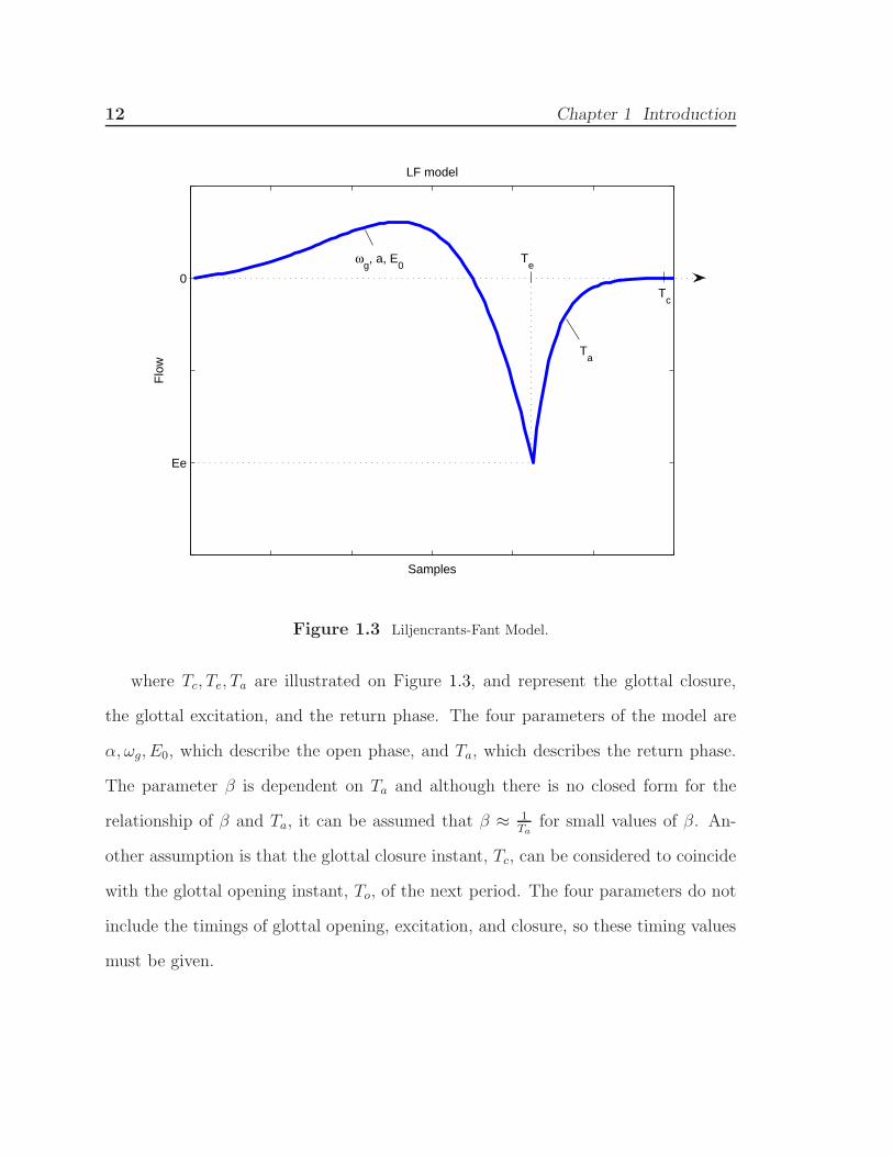
12 Chapter 1 Introduction
Ee
0
Samples
Flo
wLF model
Te
Ta
Tc
ωg, a, E
0
Figure 1.3 Liljencrants-Fant Model.
where Tc, Te, Ta are illustrated on Figure 1.3, and represent the glottal closure,
the glottal excitation, and the return phase. The four parameters of the model are
α, ωg, E0, which describe the open phase, and Ta, which describes the return phase.
The parameter β is dependent on Ta and although there is no closed form for the
relationship of β and Ta, it can be assumed that β ≈ 1Ta
for small values of β. An-
other assumption is that the glottal closure instant, Tc, can be considered to coincide
with the glottal opening instant, To, of the next period. The four parameters do not
include the timings of glottal opening, excitation, and closure, so these timing values
must be given.

1.1 Background 13
Due to the large dependence of E0 on α [53], the parameter Ee, the value of the
waveform at time Te, can be estimated instead of E0. To calculate E0 from Ee the
equation
E0 =Ee
eαTe sin(ωgTe)
is used.
The parameter Ta is the most important parameter in terms of human perception,
as it controls the amount of spectral tilt present in the source. The return phase of
the LF-model is equivalent to a first order lowpass filter [22] with a corner frequency
of
Fa =1
2πTa
The LF-model parameters and their significance is illustrated in Table 1.1.
LF model parameters
Ee The value of the waveform at time Te
α Determines the ratio of Ee to the height of
the positive portion of the glottal flow derivative
ωg Determines the curvature of the left side
of the glottal pulse.
Ta An exponential time constant which determines
how quickly the waveform returns to zero after time Te
Table 1.1 The four parameters of the Liljencrant-Fant model for the glottalflow derivative waveform.
14 Chapter 1 Introduction
1.2 Evaluation of Inverse Filtering Methods
A major obstacle both in developing new IF algorithms and in comparing existing
methods is the complication of assessing the performance of an IF technique. This
happens mostly because the signal to be estimated, the glottal flow, is unavailable.
Therefore, when IF is used to estimate the glottal flow of natural speech, it is actually
never possible to assess in detail how closely the estimated waveform corrseponds to
the true glottal flow generated by the vibrating vocal folds.
However, it is possible to use synthesized speech that has been created using artificial
glottal flow waveforms to assess the accuracy and efficiency of an IF technique. The
success of the algorithm can be judged by quantifying the error between the known
input waveform and the version recovered by the algorithm. Although this approach
is typically used in the literature [5], [6], [45], [65], [70], this kind of evaluation is not
truly objective because speech synthesis and IF analysis are based on similar models of
the human voice production system, such as the source-filter model. An improvement
would be to provide synthesized speech generated by a more sophisticated articulatory
model [34], which allows source-tract interaction [47] [8] [9]. A similar approach will
be followed in this thesis, as it will be presented later.
Once the algorithm has been verified and is being used for inverse filtering real
speech samples, there are two possible approaches to evaluate the results. One is to
compare the waveforms obtained with those obtained by earlier methods. As, typi-
cally, the aim of this is to establish that the new method is superior, the objectivity
of this approach is also doubtful. This approach can be made most objective when
methods are compared using synthetic speech and results can be compared with the
original source, as in [6]. In many works, no comparisons are made, a stance which
is not wholly unjustified because there is not enough data available to say which are
1.3 Physical Modeling of Speech Signals 15
the correct glottal flow waveforms.
On the other hand, using two different methods to extract the glottal flow could
be an effective way to confirm the appearance of the waveform as correct. If new
techniques for glottal inverse filtering produce waveforms which ’look like’ the other
waveforms that have been produced before, then they are evaluated as better than
those which do not: examples of the latter include [4], [19].
In the direction of evaluation of IF methods, a physiological-based model of vocal
folds and vocal tract is used in order to evaluate different IF methods. In this model,
time-varying waveforms of the glottal flow and radiated acoustic pressure are simu-
lated. A detailed description of this model follows next.
1.3 Physical Modeling of Speech Signals
A computational model of the vocal folds and acoustic wave propagation generated the
sound pressure and glottal flow waveforms used in this thesis. In detail, self sustained
vocal fold vibration was simulated with three masses coupled to one another through
stiffness and damping elements [60]. A schematic diagram depicting this model is
shown in Figure 1.4, where the arrangement of the masses was designed to emulate
the body-cover structure of the vocal folds [29].
The input parameters of this model are the lung pressure, prephonatory glottal
half-width (adduction), resulting vocal fold length and thickness, and normalized acti-
vation levels of the cricothyroid (CT) and thyroarytenoid (TA) muscles. These values
were transformed into mechanical parameters of the model, such as mass, stiffness,

16 Chapter 1 Introduction
Figure 1.4 Schematic diagram of the lumped-element vocal fold model. The cover-bodystructure of each vocal fold is represented by three masses that are coupled to each otherby spring and damping elements. Bilateral symmetry was assumed for all simulations.
and damping, acording to [67]. In [66], through aerodynamic and acoustic considera-
tions, the vocal fold model was coupled to the pressures and air flows in the trachea
and vocal tract. Bilateral symmetry was assumed for all simulations such that iden-
tical vibrations occur within both the left and right folds. The modification of the
resting vocal fold length and activation levels of CT and TA muscles resulted into
eight different fundamental frequency values (105, 115, 130, 145, 205, 210, 230, and 255
Hz). These values roughly approximate the range of the fundamental frequency in
adult male and female speech [30]. The input parameters for all nine cases are shown
in Table 1.2.
Acoustic wave propagation in both the trachea and vocal tract was computed in
time synchrony with the vocal fold model. This was performed with a wave-reflection
1.3 Physical Modeling of Speech Signals 17
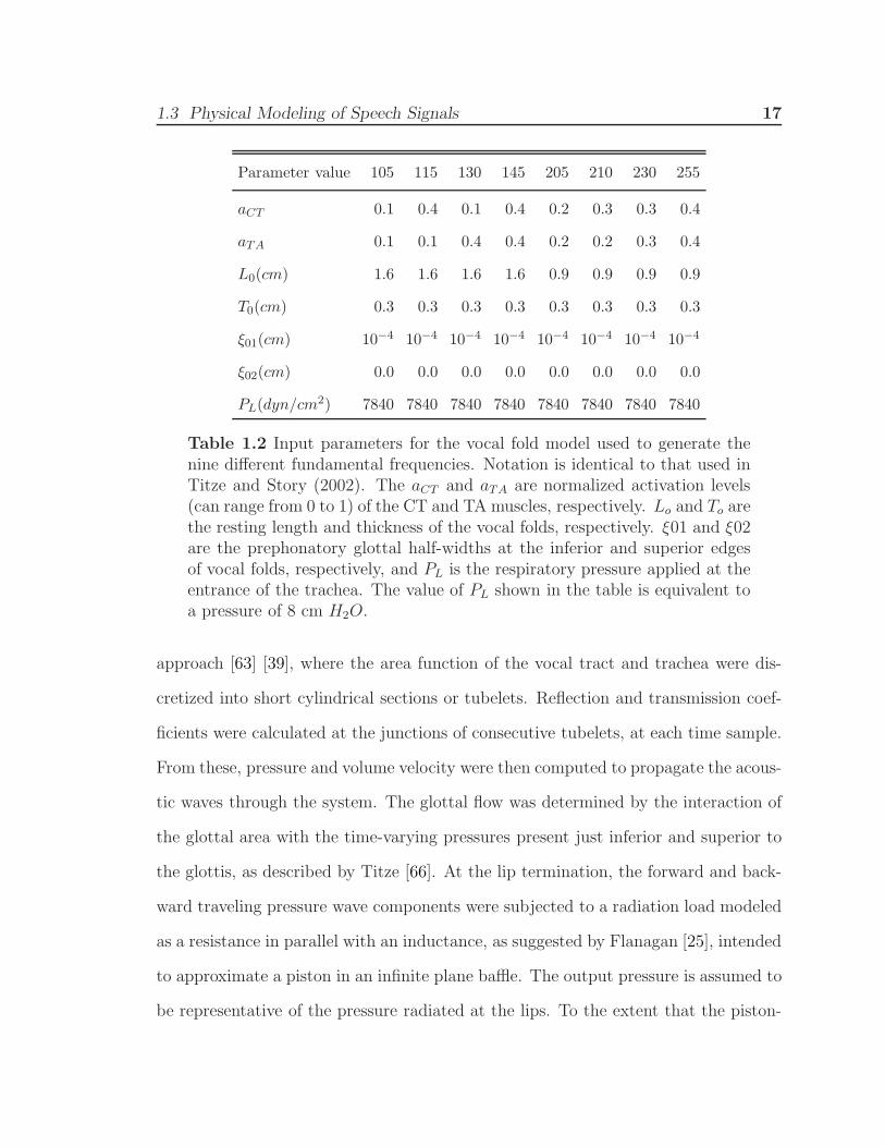
Parameter value 105 115 130 145 205 210 230 255
aCT 0.1 0.4 0.1 0.4 0.2 0.3 0.3 0.4
aTA 0.1 0.1 0.4 0.4 0.2 0.2 0.3 0.4
L0(cm) 1.6 1.6 1.6 1.6 0.9 0.9 0.9 0.9
T0(cm) 0.3 0.3 0.3 0.3 0.3 0.3 0.3 0.3
ξ01(cm) 10−4 10−4 10−4 10−4 10−4 10−4 10−4 10−4
ξ02(cm) 0.0 0.0 0.0 0.0 0.0 0.0 0.0 0.0
PL(dyn/cm2) 7840 7840 7840 7840 7840 7840 7840 7840
Table 1.2 Input parameters for the vocal fold model used to generate thenine different fundamental frequencies. Notation is identical to that used inTitze and Story (2002). The aCT and aTA are normalized activation levels(can range from 0 to 1) of the CT and TA muscles, respectively. Lo and To arethe resting length and thickness of the vocal folds, respectively. ξ01 and ξ02are the prephonatory glottal half-widths at the inferior and superior edgesof vocal folds, respectively, and PL is the respiratory pressure applied at theentrance of the trachea. The value of PL shown in the table is equivalent toa pressure of 8 cm H2O.
approach [63] [39], where the area function of the vocal tract and trachea were dis-
cretized into short cylindrical sections or tubelets. Reflection and transmission coef-
ficients were calculated at the junctions of consecutive tubelets, at each time sample.
From these, pressure and volume velocity were then computed to propagate the acous-
tic waves through the system. The glottal flow was determined by the interaction of
the glottal area with the time-varying pressures present just inferior and superior to
the glottis, as described by Titze [66]. At the lip termination, the forward and back-
ward traveling pressure wave components were subjected to a radiation load modeled
as a resistance in parallel with an inductance, as suggested by Flanagan [25], intended
to approximate a piston in an infinite plane baffle. The output pressure is assumed to
be representative of the pressure radiated at the lips. To the extent that the piston-

18 Chapter 1 Introduction
in-a-baffle reasonably approximates the radiaton load, the calculated output pressure
can also be assumed to be representative of the pressure that would be transduced by
a microphone in a non-reflective environment. The specific implementation of the vo-
cal tract model used for in this thesis was presented in Story [59], and included energy
losses due to viscosity, yielding walls, heat conduction, as well as radiation at the lips.
Figure 1.5 Area function representation of the trachea and vocal tract used to simulatethe male “a”vowel. The vocal fold model of Fig. 1.4 would be located at the 0 cm pointindicated by the dashed vertical line. Examples of the glottal flow and output pressurewaveforms are shown near the locations at which they would be generated.
In this thesis, glottal flow and speech pressure waveforms were generated for 4
vowels (/aa/, /ae/, /eh/, and /ih/) in both male and female configurations. The
area functions were taken from those reported for an adult male in Story et al [61].
For the simulations of male speech, the area functions were used directly with the
exception of the vocal tract length, which was normalized to 17.46 cm. For female
speech simulations, the same male area factors were based on those reported in Fitch

1.4 Thesis Contribution 19
and Giedd [24]. The trachea in all cases was the same as that shown in Figure 1.5.
In summary, the model is a simplified but physically motivated representation of a
speaker. It generates both the signal on which inverse filtering is typically performed
(microphone signal) and the signal that is seeked to be determined (glottal flow).
This provides an idealized test case for inverse filtering algorithms.
1.4 Thesis Contribution
In this thesis, a physiological-based model of the vocal folds and vocal tract is used
in order to evaluate different IF methods. In this model, time-varying waveforms of
the glottal flow and radiated acoustic pressure are simulated. By using this simulated
speech pressure waveform as an input to an IF method, it is possible to determnine
how close the obtained estimate of the glottal flow is to the simulated glottal flow.
This approach differs from using synthetic speech excited by an artificial glottal flow
because the glottal flow waveform results from the interaction of the self-sustained
oscillations of the vocal folds with subglottal and supraglottal pressures, as it would
happen during real speech production. Therefore, this model generates a glottal flow
waveform that is expected to provide a more firm and realistic test of the IF method
than a parametric flow model, where no source-tract interaction is taken into account.
In order to evaluate the different IF techniques, robust time and frequency do-
main parametrization measures are typically used. In this way, the most important
features of the glottal flow (or its derivative) estimates are expressed using a few nu-
merical values. The parametrization measures used in this thesis are the Normalized
Amplitude Quotient (NAQ), the Signal to Reconstruction Error ratio (SRER), the

20 Chapter 1 Introduction
difference in dB between the first two harmonics of the glottal spectrum (H1-H2),
and the Harmonic Richness Factor (HRF), which were previously discussed.
1.5 Thesis Organization
In this chapter, the basic concepts of source-filter voice production system were intro-
duced, and their relation to the inverse filtering process. The problem of evaluation of
IF techniques was illustrated, and a database of physically modeled speech pressure
signals was delineated. This database will greatly help in comparing and evaluating
different methods of IF. In Chapter 2, we will discuss the different vocal tract filter
estimation methods and their properties, as well as the inverse filtering procedure
followed for each method. Chapter 3 covers the results of each IF method, using the
measures introduced in this chapter, and finally Chapter 4 concludes the thesis and
discusses ideas for future directions in related research.
Chapter 2
Vocal Tract Filter Estimation with
Linear Prediction
As discussed in Chapter 1, most of the IF approaches suggest the use of Linear Pre-
diction Analysis in order to estimate the vocal tract filter. In this chapter, we firstly
discuss the linear prediction techniques that are used througout the rest of the thesis.
Next, we describe the inverse filtering procedure that we follow to estimate the glottal
flow waveforms.
2.1 Autocorrelation based methods
2.1.1 Classic Linear Prediction - Autocorrelation Method
If we assume that the speech signal is zero outside an interval 0 ≤ n ≤ N − 1, then
the error signal e[n] will be nonzero in the interval 0 ≤ n ≤ N + p− 1. That interval
is the region R. Since we are trying to predict nonzero samples from zero samples at
the beginning of the interval, this will result in large errors at that point. This is also
21
22 Chapter 2 Vocal Tract Filter Estimation with Linear Prediction
valid for the end of the interval, where zero samples are predicted from nonzero ones.
For this reason, a tapered window (e.g., Hamming) is often used. The forementioned
assumptions result in the autocorrelation method of linear prediction. It can be for-
mulated as follows:
By using Hamming window w[n] with lengthN , we get a windowed speech segment
sN [n], where sN [n] = s[n]w[n]. Then the mean squared prediction error is defined as:
EN =∞∑
n=−∞e2[n] =
∞∑n=−∞
(sN [n]−p∑
k=1
aksN [n− k])2. (2.1)
The values of ak that minimize EN are found by assigning the partial derivatives
of EN with respect to ak to zeros. This follows in the following p equations with p
unknown variables ak:
p∑k=1
ak
∞∑n=−∞
sN [n− i]sN [n− k] =∞∑
n=−∞sN [n− i]sN [n], 1 ≤ i ≤ p. (2.2)
Noticing that the windowed speech signal sN [n] = 0 outside the window w[n], and by
introducing the autocorrelation function
R(i) =
N−1∑n=i
sN [n]sN [n− i], 0 ≤ i ≤ p, (2.3)
equation X becomes
p∑k=1
R(|i− k|)ak = R(i), 1 ≤ i ≤ p. (2.4)
Using matrix notation, the latter equation can be written as
Φ�a = �r, (2.5)
where matrix Φ is called the autocorrelation matrix and its elements are given by
Φi,j = R(|i− j|), 1 ≤ i, j ≤ p. The other two vectors are given by
2.1 Autocorrelation based methods 23
�a = [a1, a2, a3, ..., ap]T and �r = [R(1), R(2), R(3), ..., R(p)]T .
The main advantage of the autocorrelation method is that it always produces a
stable filter with a reasonable computational load and that there are fast algorithms,
such as the Levinson-Durbin recursion algorithm [55], for solving the matrix system.
The effects of the problems at the beggining and end of the analysis region can be
reduced using a non-rectangular window, such as a Hamming window.
2.1.2 Stabilized Weighted Linear Prediction
Stabilized Weighted Linear Prediction (SWLP), introduced by Magi et al [42], is an
all-pole modeling method based on Weighted Linear Prediction (WLP) [41]. WLP
uses time domain weighting of the square of the prediction error signal. This tempo-
ral weighting emphasizes the speech samples which have a high signal-to-noise ratio,
and thus it has been shown that WLP improves the spectral envelope estimation of
noisy speech in comparison to the conventional LP analysis. Moreover, in contrast to
other robust methods of LP [40] [73], the WLP filter parameters can be calculated
without any iterative update. A problem is that the WLP filter is not guaranteed
to be stable. This drawback is dissolved through SWLP, where the weighting is such
that the all-pole model is always stable.
The formulation of WLP is presented next, as well as the SWLP algorithm that en-
sures stability of the all-pole model.

24 Chapter 2 Vocal Tract Filter Estimation with Linear Prediction
Weighted Linear Prediction
As in conventional LP, sample x[n] is estimated by a linear combination of the past
p samples:
x[n] = −p∑
i=1
aix[n− i], (2.6)
where the coefficients ai ∈ �. The prediction error en(a), the residual, is defined
as
en(a) = x[n]− x[n] = x[n] +
p∑i=1
aix[n− i] = aTx[n], (2.7)
where a = [a0a1...ap]T with a0 = 1 and x[n] = [x[n]...x[n − p]]T . The prediction
error energy E(a) in the WLP method is
E(a) =
N+p∑n=1
(en(a))2wn = aT
( N+p∑n=1
wnx[n]xT [n])a = aTRa, (2.8)
where wn is the weight imposed on sample n, N is the length of the signal x[n],
and R =∑N+p
n=1 wnx[n]xT [n]. This problem is a constrained minimization problem,
minimize E(a) subject to aTu = 1,
where u is the vector defined as u = [1 0 ... 0]T . It can be seen that the autocor-
relation matrix R is weighted, in difference to the conventional LP analysis.
Matrix R is symmetric but not Toeplitz, due to the weighting process. However, it
is positive definite, and this makes the minimization problem convex. Using Lagrange
multipliers, it can be shown that a satisfies the linear equation
Ra = σ2u, (2.9)
where σ2 = aTRa is the error energy. Finally, the WLP all-pole model is obtained
as H(z) = 1/A(z), where A(z) is the Z-transform of vector a.

2.1 Autocorrelation based methods 25
Weighting function
The time domain weighting function wn is the key point of both WLP and SWLP.
In [41], the weighting function was chosen to be the Short-Time Energy (STE)
wn =
M−1∑i=0
x2n−i−1, (2.10)
whereM is the length of the STE window. The use of STE window can be justified
as following. The STE function emphasizes the speech samples of large amplitude. It
is well-known that applying LP analysis on speech samples that belong to the glottal
closed phase interval will generally result in a more robust spectral representation of
the vocal tract. So, by emphasizing on these samples that occur during the glottal
closed phase, it is likely to yield more robust acoustical cues for the formants. In
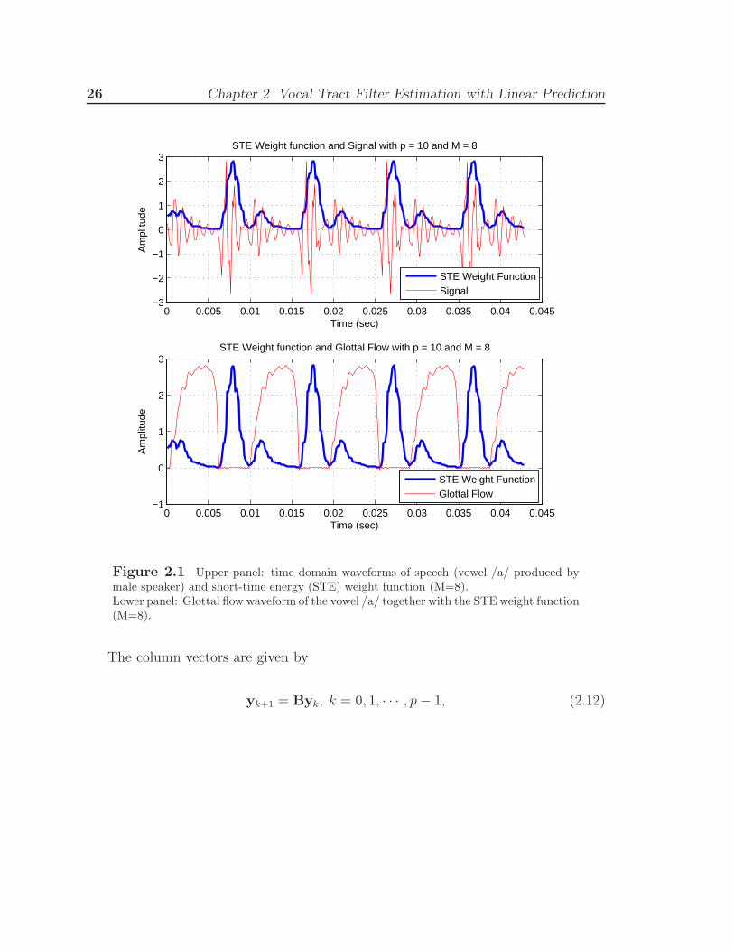
Figure 2.1, the focus on the glottal closed phase of the STE weighting function is
illustrated on a clean vowel.
Stability
However, the WLP method with the STE window does not ensure stability of the
all-pole model. Therefore, in [42], a formula for a generalized weighting function to
be used in WLP is developed in order to guarantee stability. The autocorrelation
matrix R in Eq. X can be expressed as
R = YTY, (2.11)
where
Y = [y0 y1 · · ·yp] ∈ �(N+p)x(p+1)
and
y0 = [√w1x[1] · · ·√wNx[N ] 0 · · ·0]T .
26 Chapter 2 Vocal Tract Filter Estimation with Linear Prediction
0 0.005 0.01 0.015 0.02 0.025 0.03 0.035 0.04 0.045−3
−2
−1
0
1
2
3STE Weight function and Signal with p = 10 and M = 8
Time (sec)
Am
plitu
de
STE Weight FunctionSignal
0 0.005 0.01 0.015 0.02 0.025 0.03 0.035 0.04 0.045−1
0
1
2
3STE Weight function and Glottal Flow with p = 10 and M = 8
Time (sec)
Am
plitu
de
STE Weight FunctionGlottal Flow
Figure 2.1 Upper panel: time domain waveforms of speech (vowel /a/ produced bymale speaker) and short-time energy (STE) weight function (M=8).Lower panel: Glottal flow waveform of the vowel /a/ together with the STE weight function(M=8).
The column vectors are given by
yk+1 = Byk, k = 0, 1, · · · , p− 1, (2.12)
2.2 Covariance based methods 27
where
B =
⎡⎢⎢⎢⎢⎢⎢⎢⎢⎢⎢⎢⎣
0 0 · · · 0 0√w2/w1 0 0 · · · 0
0√w3/w2 0 · · · 0
.... . .
. . .. . .
...
0 · · · 0√wN+p/wN+p−1 0
⎤⎥⎥⎥⎥⎥⎥⎥⎥⎥⎥⎥⎦
So, before forming the matrixY, the elements of the secondary diagonal of the matrix
B are defined for all i = 1, · · · , N + p− 1 as
Bi+1,i =
⎧⎪⎨⎪⎩
√wi+1/wi, if wi ≤ wi+1
1, if wi > wi+1
Finally, the WLP method computed using matrix B is called the Stabilized Weighted
Linear Prediction model, and the stability of the all-pole filter is ensured. For more
information on the stability of SWLP, see [42].
2.2 Covariance based methods
2.2.1 Classic Linear Prediction - Covariance Method
If we assume that the speech signal is zero outside an interval p ≤ n ≤ N − 1, thus
p samples outside the region are available, then the mean squared prediction error is
given by
EN =
N−1∑m=0
e2[m] (2.13)
28 Chapter 2 Vocal Tract Filter Estimation with Linear Prediction
where e[m] = s[m] −p∑
k=1
aks[m − k], 0 ≤ m ≤ N − 1 and the interval [0, N − 1] is
the prediction error interval.
Using a similar approach with the autocorrelation method in minimizing the pre-
diction error, we result in the covariance method of linear prediction, which is given
by the following equation:
Φ�a = �ψ, (2.14)
where the elements of the covariance matrix Φ are given by
φi,j =
N−1∑n=0
s[n− i]s[n− j], (2.15)
where 1 ≤ i ≤ p and 1 ≤ j ≤ p. The other two vectors are given by
�a = [a1, a2, a3, ..., ap]T , �ψ = [φ0,1, φ0,2, φ0,3, ..., φ0,p]
T . (2.16)
Matrix Φ has the properties of a covariance matrix and thus the system can be
efficiently solved using Cholesky Decomposition.
The main advantage of the covariance method is that it always results in the cor-
rect solution for any window length greater than p. Also, if the boundaries of the
window are handled properly, a rectangular window can be used. Finally, the main
disadvantage of this method is that stability of the filter is not always guaranteed.
It should also be noted that in high pitched speakers, the closed phase interval is
typically too short, and thus the estimation of the vocal tract filter is not accurate.
This yields severe distortions on the estimated glottal flow, such as increased ripple
in its closed phase interval.
2.2 Covariance based methods 29
As it was mentioned in Chapter 1, it is advantageous to restrict the analysis re-
gion in the closed phase interval of the glottal flow waveform. This approach is called
Closed Phase (CP) Covariance LP Analysis and it is the covariance technique that
is tested in this thesis.
2.2.2 Constrained Closed Phase Covariance Linear Predic-
tion
Problems with conventional CP covariance analysis
The classic CP covariance LP analysis described in the previous section suffers from
certain shortcomings. Several previous studies [38] [69] [72] [57] indicate that the CP
analysis is very sensitive to the position of the covariance frame, thus giving glottal
flow estimated that vary greatly. This is understandable if we consider that CP length
is typically short, and the amount of data used to define the parametric model of the
vocal tract is sparse. If the position of this frame is misaligned, then this results in
poor modeling of the vocal tract resonances, and thus severe distortion of the glottal
flow estimates. The problem is more apparent in high pitch speakers, where the length
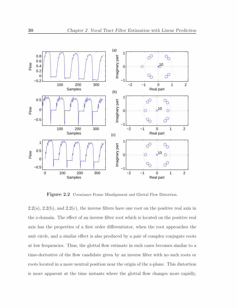
of the CP interval is very short. This type of distortion is demonstrated in Figure 2.2.
In this figure, three glottal flow estimates are shown on the left, which were inverse
filtered from the same token of a male subject uttering the vowel [a], by using a mi-
nor change in the position of the covariance frame. This example shows how a minor
change in the position of the covariance frame has resulted in a major change in the
glottal flow estimates. On the right of this figure, the corresponding pole-root loca-
tions of the glottal flow estimates are shown. It is interesting to notice that in Figs.
30 Chapter 2 Vocal Tract Filter Estimation with Linear Prediction
100 200 300−0.2
00.20.40.60.8
Flo
w
Samples
100 200 300
−0.5
0
0.5
Flo
w
Samples
0 100 200 300
−0.5
0
0.5
1
Flo
w
Samples
−2 −1 0 1 2−1
0
1
10
Real part
Imag
inar
y pa
rt
−2 −1 0 1 2−1
0
1
10
Real part
Imag
inar
y pa
rt
−2 −1 0 1 2−1
0
1
10
Real part
Imag
inar
y pa
rt
(a)
(b)
(c)
Figure 2.2 Covariance Frame Misalignment and Glottal Flow Distortion.
2.2(a), 2.2(b), and 2.2(c), the inverse filters have one root on the positive real axis in
the z-domain. The effect of an inverse filter root which is located on the positive real
axis has the properties of a first order differentiator, when the root approaches the
unit circle, and a similar effect is also produced by a pair of complex conjugate roots
at low frequencies. Thus, the glottal flow estimate in such cases becomes similar to a
time-derivative of the flow candidate given by an inverse filter with no such roots or
roots located in a more neutral position near the origin of the z-plane. This distortion
is more apparent at the time instants where the glottal flow changes more rapidly,
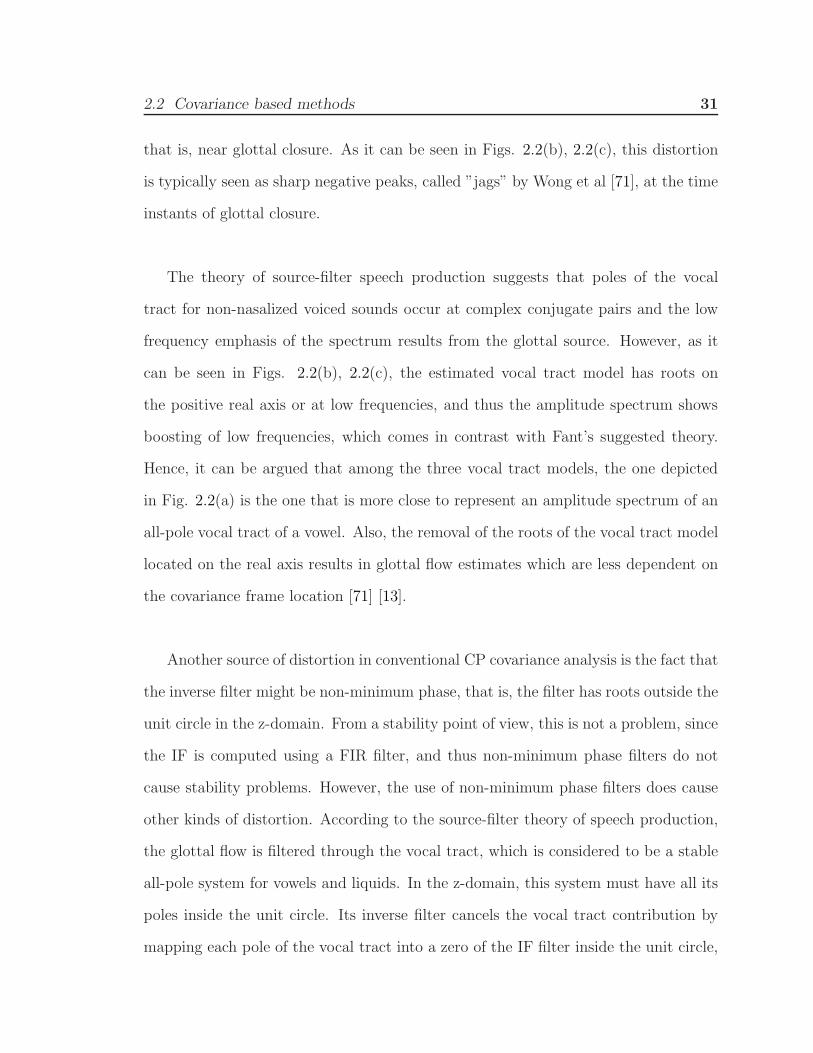
2.2 Covariance based methods 31
that is, near glottal closure. As it can be seen in Figs. 2.2(b), 2.2(c), this distortion
is typically seen as sharp negative peaks, called ”jags” by Wong et al [71], at the time
instants of glottal closure.
The theory of source-filter speech production suggests that poles of the vocal
tract for non-nasalized voiced sounds occur at complex conjugate pairs and the low
frequency emphasis of the spectrum results from the glottal source. However, as it
can be seen in Figs. 2.2(b), 2.2(c), the estimated vocal tract model has roots on
the positive real axis or at low frequencies, and thus the amplitude spectrum shows
boosting of low frequencies, which comes in contrast with Fant’s suggested theory.
Hence, it can be argued that among the three vocal tract models, the one depicted
in Fig. 2.2(a) is the one that is more close to represent an amplitude spectrum of an
all-pole vocal tract of a vowel. Also, the removal of the roots of the vocal tract model
located on the real axis results in glottal flow estimates which are less dependent on
the covariance frame location [71] [13].
Another source of distortion in conventional CP covariance analysis is the fact that
the inverse filter might be non-minimum phase, that is, the filter has roots outside the
unit circle in the z-domain. From a stability point of view, this is not a problem, since
the IF is computed using a FIR filter, and thus non-minimum phase filters do not
cause stability problems. However, the use of non-minimum phase filters does cause
other kinds of distortion. According to the source-filter theory of speech production,
the glottal flow is filtered through the vocal tract, which is considered to be a stable
all-pole system for vowels and liquids. In the z-domain, this system must have all its
poles inside the unit circle. Its inverse filter cancels the vocal tract contribution by
mapping each pole of the vocal tract into a zero of the IF filter inside the unit circle,
32 Chapter 2 Vocal Tract Filter Estimation with Linear Prediction
this resulting in a minimum phase filter. However, it is well-known in the theory of
digital signal processing that a zero of a FIR filter can be mirrored, that is, it can be
replaced by its mirror image partner. A zero at z = z0 can be replaced by a zero at
z = 1/z∗0 , without changing the shape of the amplitude spectrum of the filter. Hence,
from an inverse filtering point of view, there are several inverse filters: one of them
is minimum phase and the others are non-minimum phase, and all of them are con-
sidered equal. These filters, however, are different in terms of phase characteristics.
This difference can cause severe distortion, and it is particularly strong in cases where
zeros of the inverse filter located in the vicinity of the lowest two formants are moved
from inside to outside the unit circle.
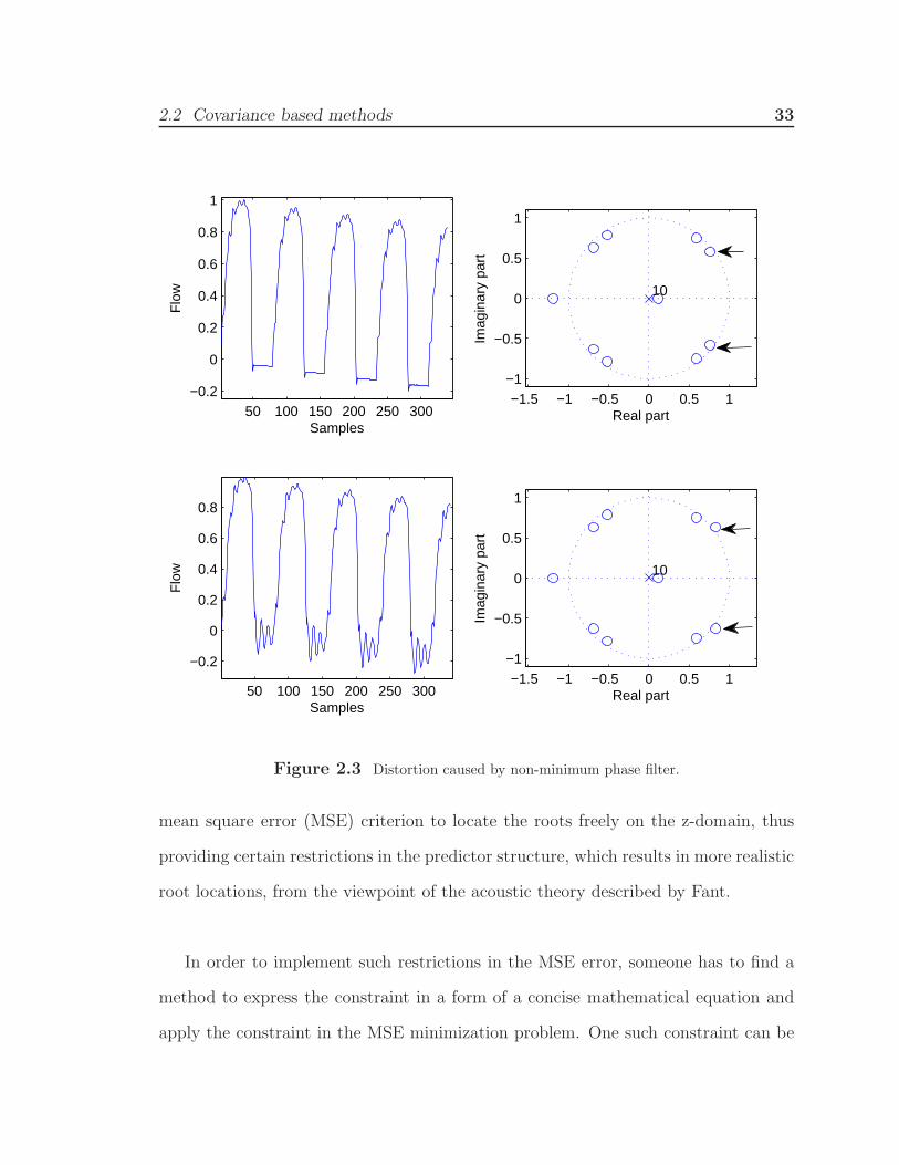
Figure 2.3 demonstrates this distortion caused by IF a vowel waveform with a
minimum and a non-minimum phase FIR filter. In Fig. 2.3(a), the glottal flow es-
timated with a minimum phase filter is shown on the left, and the corresponding
z-plane representation is shown on the right. In Fig. 2.3(b), the complex conjugate
root pair that models the first formant is replaced by its counterpart outside the unit
circle. Even though this slight modification only changed the root radius by 0.04, the
distortion caused in the glottal flow estimate is severe and is displayed as increased
ripple during the closed phase interval of the glottal cycle, as shown in the left panel
of Fig. 2.3(b).
Mathematically Constrained Linear Prediction
The concept of mathematically constrained linear prediction is the modification of
the conventional covariance analysis in order to reduce the distortion which is caused
by unrealistic vocal tract model roots location. This is achieved by not allowing the
2.2 Covariance based methods 33
50 100 150 200 250 300−0.2
0
0.2
0.4
0.6
0.8
1
Flo
w
Samples
−1.5 −1 −0.5 0 0.5 1−1
−0.5
0
0.5
1
10
Real part
Imag
inar
y pa
rt
50 100 150 200 250 300
−0.2
0
0.2
0.4
0.6
0.8
Flo
w
Samples
−1.5 −1 −0.5 0 0.5 1−1
−0.5
0
0.5
1
10
Real part
Imag
inar
y pa
rt
Figure 2.3 Distortion caused by non-minimum phase filter.
mean square error (MSE) criterion to locate the roots freely on the z-domain, thus
providing certain restrictions in the predictor structure, which results in more realistic
root locations, from the viewpoint of the acoustic theory described by Fant.
In order to implement such restrictions in the MSE error, someone has to find a
method to express the constraint in a form of a concise mathematical equation and
apply the constraint in the MSE minimization problem. One such constraint can be

34 Chapter 2 Vocal Tract Filter Estimation with Linear Prediction
expressed with the help of the DC gain of the LP filter. The DC gain can be expressed
as the sum of the predictor coefficients
V (ej0) =
p∑k=0
αk = lDC . (2.17)
where αk are the filter coefficients of the constrained inverse filter and the lDC is a
pre-defined real value for the gain of the filter at DC. The reason for selecting the con-
straint on the DC gain is that, without it, it is possible that the amplitude response
of the vocal tract model shows excessive boost at zero frequency. It is known from
Fant’s suggested source-filter theory, that the amplitude response of voiced sounds
approaches unity at zero frequency [21]. Therefore, if a misplaced and short covari-
ance frame occurs, it might even lead to an amplitude response with larger gain at
zero frequency than at formants, which is a clear violation of the source-filter theory
and its underlying acoustical theory of tube shapes. By imposing this constraint on
the DC gain of the covariance linear prediction analysis, one might expect that the
amplitude response of the resulting vocal tract estimates will better match Fant’s
source-filter theory.
However, it should be noted that this method still leaves the determination of
the exact z-domain root locations of the vocal tract model to the MSE criterion, and
does not bias the root locations prior the optimization. The formulation of the DC-
constrained LP follows.
A mathematically straightforward way to implement such a restriction in the
conventional LP, as it is described in a previous section, is to set a certain pre-defined
value for the frequency response of the all-pole model at zero frequency, as it is written
in Eq. 2.17. Using matrix notation, the DC-constrained minimization problem can
2.2 Covariance based methods 35
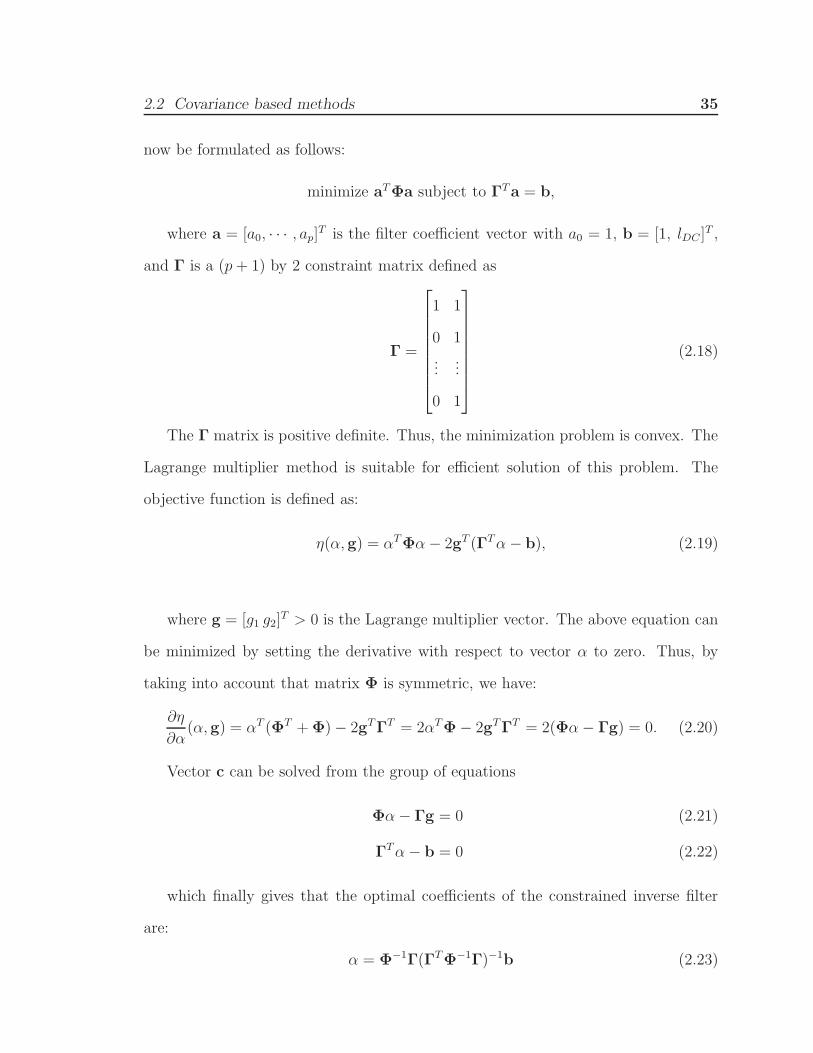
now be formulated as follows:
minimize aTΦa subject to ΓTa = b,
where a = [a0, · · · , ap]T is the filter coefficient vector with a0 = 1, b = [1, lDC ]T ,
and Γ is a (p+ 1) by 2 constraint matrix defined as
Γ =
⎡⎢⎢⎢⎢⎢⎢⎢⎣
1 1
0 1
......
0 1
⎤⎥⎥⎥⎥⎥⎥⎥⎦
(2.18)
The Γ matrix is positive definite. Thus, the minimization problem is convex. The
Lagrange multiplier method is suitable for efficient solution of this problem. The
objective function is defined as:
η(α, g) = αTΦα− 2gT (ΓTα− b), (2.19)
where g = [g1 g2]T > 0 is the Lagrange multiplier vector. The above equation can
be minimized by setting the derivative with respect to vector α to zero. Thus, by
taking into account that matrix Φ is symmetric, we have:
∂η
∂α(α, g) = αT (ΦT +Φ)− 2gTΓT = 2αTΦ− 2gTΓT = 2(Φα− Γg) = 0. (2.20)
Vector c can be solved from the group of equations
Φα− Γg = 0 (2.21)
ΓTα− b = 0 (2.22)
which finally gives that the optimal coefficients of the constrained inverse filter
are:
α = Φ−1Γ(ΓTΦ−1Γ)−1b (2.23)
36 Chapter 2 Vocal Tract Filter Estimation with Linear Prediction
0 0.1 0.2 0.3 0.4 0.5 0.6 0.7 0.8 0.9 1−15
−10
−5
0
5
10
15
20
25
Normalized Frequency (×π rad/sample)
Mag
nitu
de (
dB)
Constr. at ω = 0 and ω = π CP CovarianceConventional CP Covariance
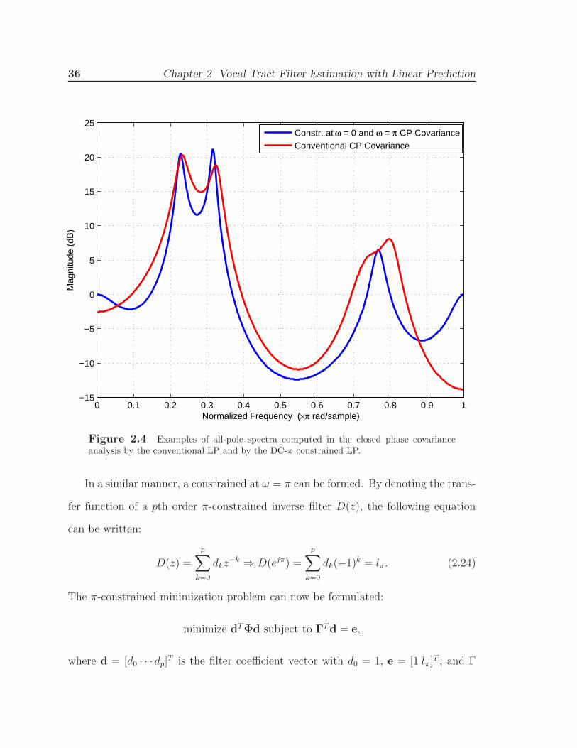
Figure 2.4 Examples of all-pole spectra computed in the closed phase covarianceanalysis by the conventional LP and by the DC-π constrained LP.
In a similar manner, a constrained at ω = π can be formed. By denoting the trans-
fer function of a pth order π-constrained inverse filter D(z), the following equation
can be written:
D(z) =
p∑k=0
dkz−k ⇒ D(ejπ) =
p∑k=0
dk(−1)k = lπ. (2.24)
The π-constrained minimization problem can now be formulated:
minimize dTΦd subject to ΓTd = e,
where d = [d0 · · · dp]T is the filter coefficient vector with d0 = 1, e = [1 lπ]T , and Γ

2.2 Covariance based methods 37
the new (p+ 1) by 2 constraint matrix is defined as:
Γ =
⎡⎢⎢⎢⎢⎢⎢⎢⎢⎢⎢⎢⎢⎢⎢⎣
1 1
0 −1
0 1
0 −1
......
0 1
⎤⎥⎥⎥⎥⎥⎥⎥⎥⎥⎥⎥⎥⎥⎥⎦
(2.25)
It is also possible to assign a third constraint by imposing simultaneously that
the first inverse filter coefficient is equal to unity and that the filter gain at both
ω = 0 and ω = π are equal to lDC and lπ respectively. Then, the constraint equation
becomes ΓTv = h, where v = [v0 · · · vp]T is the filter coefficient vector with v0 = 1,
h = [1 lDC lπ] and the resulting (p+ 1) by 3 constraint matrix is defined as:
Γ =
⎡⎢⎢⎢⎢⎢⎢⎢⎢⎢⎢⎢⎢⎢⎢⎣
1 1 1
0 1 −1
0 1 1
0 1 −1
......
0 1 1
⎤⎥⎥⎥⎥⎥⎥⎥⎥⎥⎥⎥⎥⎥⎥⎦
(2.26)
An example of the vocal tract filter estimations during a closed phase region for
the Constrained Covariance method and the conventional one is depicted in Figure
2.4.
38 Chapter 2 Vocal Tract Filter Estimation with Linear Prediction
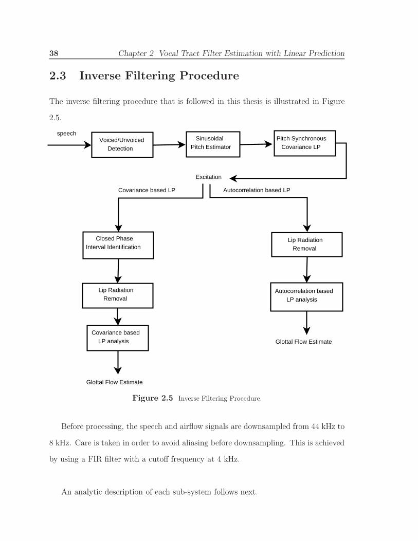
2.3 Inverse Filtering Procedure
The inverse filtering procedure that is followed in this thesis is illustrated in Figure
2.5.
Voiced/Unvoiced Detection
speech Sinusoidal Pitch Estimator
Pitch Synchronous Covariance LP
Excitation
Covariance based LP Autocorrelation based LP
Closed Phase Interval Identification
Autocorrelation based LP analysis
Glottal Flow Estimate
Lip Radiation Removal
Lip Radiation Removal
Covariance based LP analysis
Glottal Flow Estimate
Figure 2.5 Inverse Filtering Procedure.
Before processing, the speech and airflow signals are downsampled from 44 kHz to
8 kHz. Care is taken in order to avoid aliasing before downsampling. This is achieved
by using a FIR filter with a cutoff frequency at 4 kHz.
An analytic description of each sub-system follows next.

2.3 Inverse Filtering Procedure 39
2.3.1 VUS detector
As first, the speech waveforms generated by physical modeling of the vocal tract
are passed through a voiced/unvoiced/silence (VUS) detection algorithm in order to
cut any silent or unvoiced regions. Any VUS detection algorithm can be used at
this point, but one based on energy and zero crossings is preferred here due to its
simplicity, low complexity, and speed. The analysis is performed small segments of
speech, with 30 ms of duration and a 15 ms of overlap between successive segments.
2.3.2 Pitch Estimation
Afterwards, an estimate of the pitch of the voiced parts of the waveform is obtained.
Although any pitch estimator can be used in this part, the sinusoidal pitch estima-
tor [44] is used here. Pitch estimates are calculated on a speech frame of 30 ms with
a 15 ms overlap.
2.3.3 Excitation Instants Detection
According to the pitch estimates generated by the previous algorithm, a pitch-synchronous
covariance-based LP analysis on the waveform is performed, with an order of p = 10,
for speech signals with sampling frequency Fs = 8 kHz. The purpose of this analysis
is not an accurate estimate of the vocal tract or the glottal flow in each frame, but
a rough approximation of the excitation and the glottal excitation instants, which
indicate glottal closure. The reason for this analysis is the identification of pitch pe-
riods throughout the whole speech signal and it is an initial step for CP covariance

40 Chapter 2 Vocal Tract Filter Estimation with Linear Prediction
analysis, as it will be shown later.
After this point, the analysis differs depending on the LP method that is used.
2.3.4 Covariance-based LP Analysis
For CP covariance-based methods, it is necessary to identify the closed phase inter-
val. This is achieved by using the sliding covariance analysis suggested by Plumpe et
al [53], which provides a robust method to extract the glottal closed phase interval
out of the speech signal. Specifically, this method of glottal closed phase estimation
relies on a sliding covariance analysis and uses vocal tract formant modulation which
is predicted by Ananthapadmanabha and Fant [2] to vary more slowly in the glottal
closed phase than in its open phase and to respond quickly to a change in glottal area.
A ”stationary” region of formant modulation gives a closed-phase time interval, over
which we estimate the vocal tract transfer function. A stationary region is present
even when the vocal folds remain partly open [53]. For high pitch speakers, where the
closed phase samples are less than twice the order of the LP analysis, a fixed length
of NCP + order closed phase samples was used.
Then, before inverse filtering, the lip radiation is cancelled using a first order
all-pole filter with its pole at z = 0.999. Having the closed phase intervals for each
period, a covariance-based LP analysis with order p = 10 is set up on the correspond-
ing speech samples. Finally, the vocal tract estimate that is obtained inverse filters
pitch synchronously a speech segment consisting of two pitch periods, and thus the
glottal flow is obtained.
2.4 Summary 41
2.3.5 Autocorrelation-based LP Analysis
For autocorrelation based methods, the analysis is simpler. The lip radiation is can-
celled using a first order all-pole filter with its pole at z = 0.999. Next, using the
glottal pulses identified in a previous step, a pitch-synchronous LP analysis with order
p = 10 is performed over a speech segment of 250 ms. The vocal tract contribution is
then cancelled by inverse filtering over a region of two pitch periods, with an overlap
of one pitch period.
The overall glottal flow is synthesized using the well-known Overlap-Add method
(OLA) [55].
2.4 Summary
In this chapter, four LP-based spectral estimation techniques were discussed and
applied to an inverse filtering process; two of them are well-kwown and widely used:
the conventional autocorrelation and covariance LP. The other two were recently
developed and they are referred to as Stabilised Weighted Linear Prediction and
Constrained Closed Phase Covariance LP. SWLP is suggested for IF since it has the
interesting property of emphasizing the speech samples that typically occur during the
closed phase region. Finally, an automatic system for inverse filtering was described.

42 Chapter 2 Vocal Tract Filter Estimation with Linear Prediction
Chapter 3
Results
In this chapter, we firstly present glottal flow estimates of several vowels of different
frequencies, using the IF techniques described in Chapter 2. Then, parametrization
measures in time and frequency domain are applied on the estimates, in order to
compare and evaluate the performance of different IF techniques. Finally, comments
are presented on both the shape of the glottal flow estimates and the parametrization
measures.
3.1 Glottal Flow Estimates Examples
The database consists of four physically modeled speech waveforms, all vowels (/aa/,
/ae/, /eh/, /ih/), each one in eight different frequencies (105, 115, 130, 145, 205, 210, 230,
and 255 Hz). That is a total of 32 speech signals. For brevity, we present here char-
acteristic examples for each of the five vowels. In each figure (from left to right), we
show first the actual glottal flow waveform, which is encapsulated by a thick-line box.
Then, it follows the estimates using the autocorrelation-based LPC IF technique,
43

44 Chapter 3 Results
the Stabilized Weighted LPC IF technique with parameter M = 8, the Stabilized
Weighted LPC IF technique with parameter M = 24, the covariance-based LPC IF
technique, and finally the constrained covariance-based LPC IF technique.
400 450 500 550 600
0
0.5
1
Actual glottal flow
400 450 500 550 600
0
0.5
1
Autocorr−LPC
400 450 500 550 600
0
0.5
1
SW−LPC, M=8
400 450 500 550 600
0
0.5
1
SW−LPC, M=24
400 450 500 550 600
0
0.5
1
Covariance−LPC
400 450 500 550 600
0
0.5
1
Constr. Covariance−LPC
Figure 3.1 Glottal flow estimates for vowel /aa/, fundamental frequency of 105 Hz.
As it can be seen in the figures, the estimated glottal flow waveforms are, in gen-
eral, close to the original one. However, the best fit is achieved by the CP covariance
methods, because of a more accurate extraction of the vocal tract filter during the
closed phase interval. Also, the SWLP24 waveform, which corresponds to the SWLP

3.2 Parametrization Results 45
400 450 500 550 600
0
0.5
1
Actual glottal flow
400 450 500 550 600
0
0.5
1
Autocorr−LPC
400 450 500 550 600
0
0.5
1
SW−LPC, M=8
400 450 500 550 600
0
0.5
1
SW−LPC, M=24
400 450 500 550 600
0
0.5
1
Covariance−LPC
400 450 500 550 600
0
0.5
1
Constr. Covariance−LPC
Figure 3.2 Glottal flow estimates for vowel /aa/, fundamental frequency of 145 Hz.
with M = 24, is closer to the original one, compared to the autocorrelation method
of LP.
3.2 Parametrization Results
In order to parametrize our results, the previously discussed time and frequency do-
main measures were applied on the glottal flow estimates. In this chapter, the IF
methods are abbreviated as: WLPC8 stands for Stabilized Weighted Linear Predic-

46 Chapter 3 Results
400 500 600 700 800
0
0.5
1
Actual glottal flow
400 500 600 700 800
0
0.5
1
Autocorr−LPC
400 500 600 700 800
0
0.5
1
SW−LPC, M=8
400 500 600 700 800
0
0.5
1
SW−LPC, M=24
400 500 600 700 800
0
0.5
1
Covariance−LPC
400 500 600 700 800
0
0.5
1
Constr. Covariance−LPC
Figure 3.3 Glottal flow estimates for vowel /ae/, fundamental frequency of 145 Hz.
tion with STE window of length M = 8, WLPC24 stands for Stabilized Weighted
Linear Prediction with STE window of length M = 24, LPC stands for the con-
ventional autocorrelation Linear Prediction, CovLPC stands for the conventional CP
covariance Linear Prediction and CLPC stands for the Constrained CP covariance
Linear Prediction.
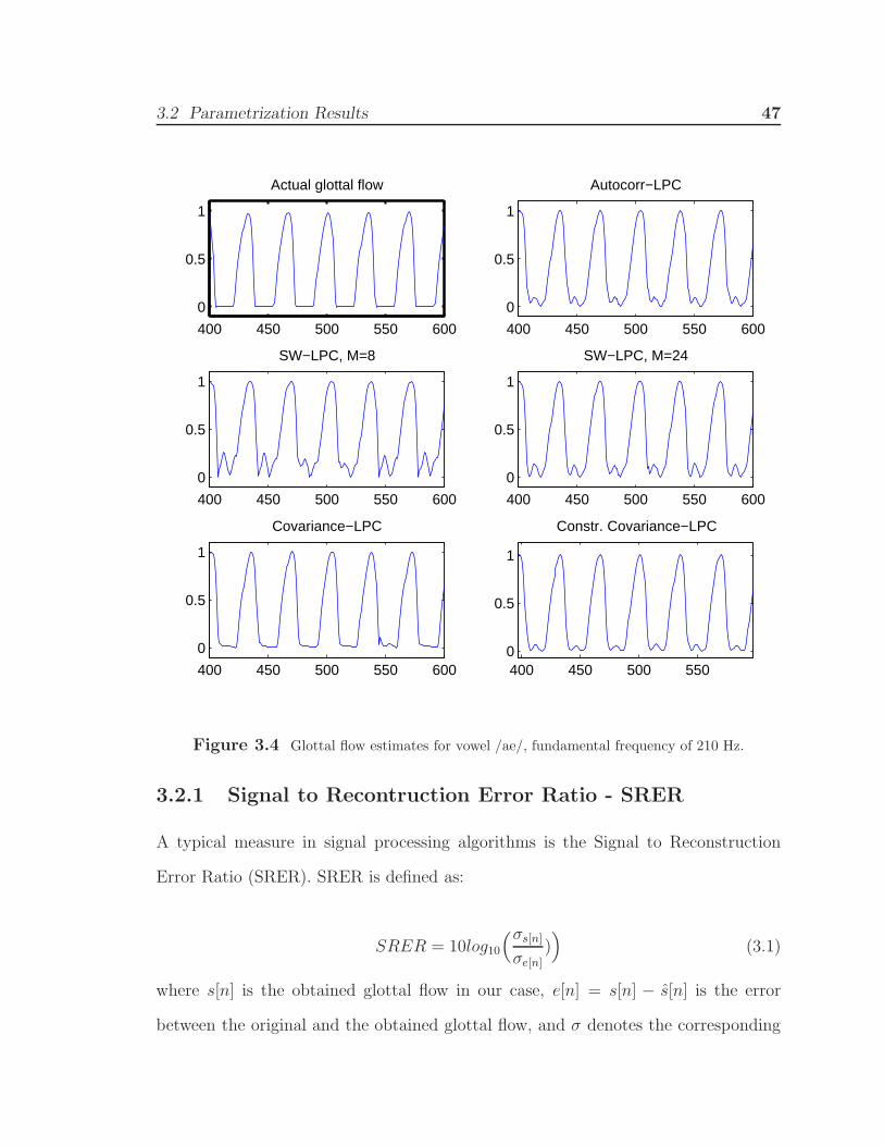
3.2 Parametrization Results 47
400 450 500 550 600
0
0.5
1
Actual glottal flow
400 450 500 550 600
0
0.5
1
Autocorr−LPC
400 450 500 550 600
0
0.5
1
SW−LPC, M=8
400 450 500 550 600
0
0.5
1
SW−LPC, M=24
400 450 500 550 600
0
0.5
1
Covariance−LPC
400 450 500 5500
0.5
1
Constr. Covariance−LPC
Figure 3.4 Glottal flow estimates for vowel /ae/, fundamental frequency of 210 Hz.
3.2.1 Signal to Recontruction Error Ratio - SRER
A typical measure in signal processing algorithms is the Signal to Reconstruction
Error Ratio (SRER). SRER is defined as:
SRER = 10log10
(σs[n]σe[n]
))
(3.1)
where s[n] is the obtained glottal flow in our case, e[n] = s[n] − s[n] is the error
between the original and the obtained glottal flow, and σ denotes the corresponding

48 Chapter 3 Results
400 500 600 700 800
0
0.5
1
Actual glottal flow
400 500 600 700 800
0
0.5
1
Autocorr−LPC
400 500 600 700 800
0
0.5
1
SW−LPC, M=8
400 500 600 700 800
0
0.5
1
SW−LPC, M=24
400 500 600 700 800
0
0.5
1
Covariance−LPC
400 450 500 550 600
0
0.5
1
Constr. Covariance−LPC
Figure 3.5 Glottal flow estimates for vowel /ih/, fundamental frequency of 115 Hz.
standard deviation. SRER is a means to estimate how well the estimated glottal flow
”fits” on the original one. In other words, it is an index of the quality of the pitch
synchronously resynthesized glottal flow waveform.
Table 3.1 shows the mean and the standard deviation of SRER for each IF method
per vowel.
In table 3.1, it is clearly seen that the CP covariance methods outperform the au-
tocorrelation methods in terms of the SRER. However, CP covariance methods shows
a small decrease in performance for the /ih/ vowel. This can be justified by the fact
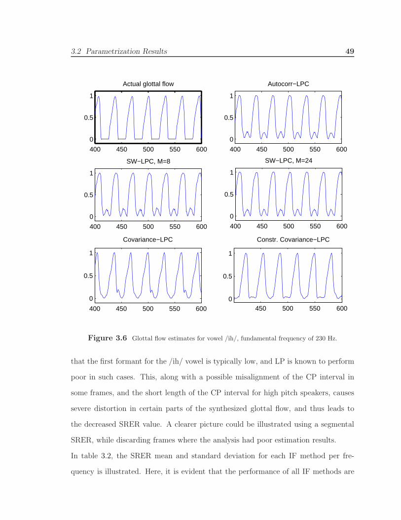
3.2 Parametrization Results 49
400 450 500 550 600
0
0.5
1
Actual glottal flow
400 450 500 550 600
0
0.5
1
Autocorr−LPC
400 450 500 550 600
0
0.5
1
SW−LPC, M=8
400 450 500 550 600
0
0.5
1
SW−LPC, M=24
450 500 550 6000
0.5
1
Constr. Covariance−LPC
400 450 500 550 600
0
0.5
1
Covariance−LPC
Figure 3.6 Glottal flow estimates for vowel /ih/, fundamental frequency of 230 Hz.
that the first formant for the /ih/ vowel is typically low, and LP is known to perform
poor in such cases. This, along with a possible misalignment of the CP interval in
some frames, and the short length of the CP interval for high pitch speakers, causes
severe distortion in certain parts of the synthesized glottal flow, and thus leads to
the decreased SRER value. A clearer picture could be illustrated using a segmental
SRER, while discarding frames where the analysis had poor estimation results.
In table 3.2, the SRER mean and standard deviation for each IF method per fre-
quency is illustrated. Here, it is evident that the performance of all IF methods are
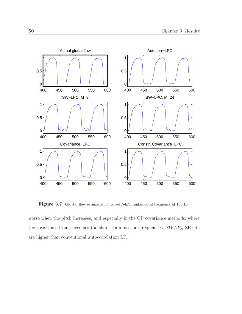
50 Chapter 3 Results
400 450 500 550 600
0
0.5
1
Actual glottal flow
400 450 500 550 600
0
0.5
1
Autocorr−LPC
400 450 500 550 600
0
0.5
1
SW−LPC, M=8
400 450 500 550 600
0
0.5
1
SW−LPC, M=24
400 450 500 550 600
0
0.5
1
Covariance−LPC
400 450 500 550 600
0
0.5
1
Constr. Covariance−LPC
Figure 3.7 Glottal flow estimates for vowel /eh/, fundamental frequency of 105 Hz.
worse when the pitch increases, and especially in the CP covariance methods, where
the covariance frame becomes too short. In almost all frequencies, SWLP24 SRERs
are higher than conventional autocorrelation LP.

3.2 Parametrization Results 51
400 450 500 550 600
0
0.5
1
Actual glottal flow
400 450 500 550 600
0
0.5
1
Autocorr−LPC
400 450 500 550 600
0
0.5
1
SW−LPC, M=8
400 450 500 550 600
0
0.5
1
SW−LPC, M=24
400 450 500 550 600
0
0.5
1
Constr. Covariance−LPC
400 450 500 550 600
0
0.5
1
Covariance−LPC
Figure 3.8 Glottal flow estimates for vowel /eh/, fundamental frequency of 255 Hz.
3.2.2 Normalized Amplitude Quotient - NAQ
For the synthesized glottal flows, the NAQ was estimated for each cycle. In order to
compare the NAQ values of the original and the estimated glottal flows, the ratio of
the NAQ of the actual glottal flow to the estimated one is formed, called NAQrat. The
ratio should be equal to unity when the estimation of the glottal flow has succeeded
perfectly.
Table 3.3 shows the mean and the standard deviation of NAQrat for each IF method
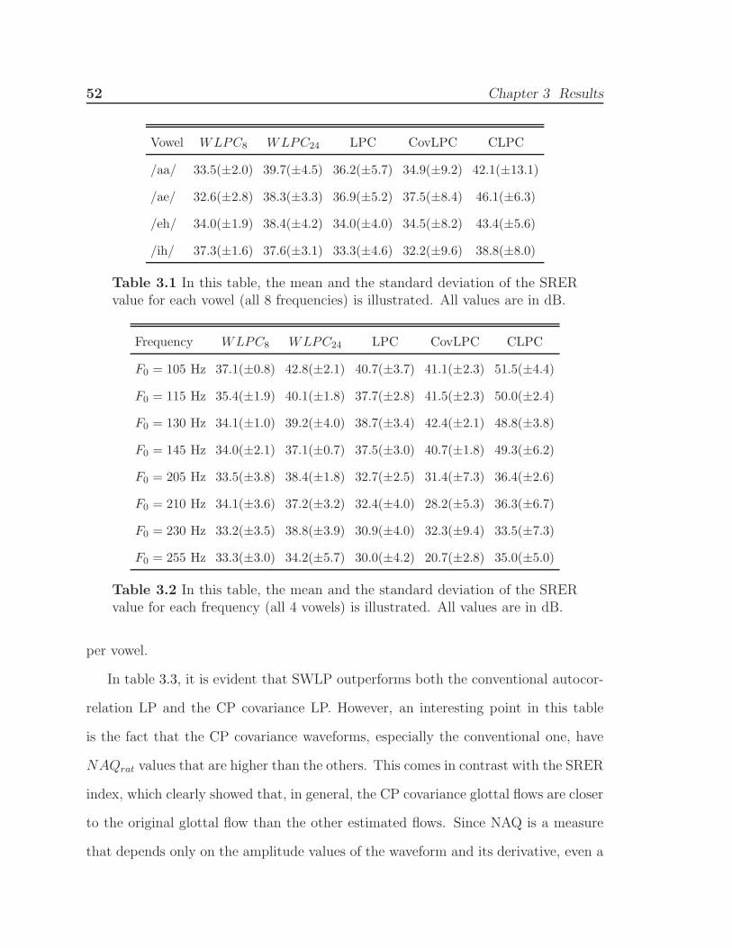
52 Chapter 3 Results
Vowel WLPC8 WLPC24 LPC CovLPC CLPC
/aa/ 33.5(±2.0) 39.7(±4.5) 36.2(±5.7) 34.9(±9.2) 42.1(±13.1)
/ae/ 32.6(±2.8) 38.3(±3.3) 36.9(±5.2) 37.5(±8.4) 46.1(±6.3)
/eh/ 34.0(±1.9) 38.4(±4.2) 34.0(±4.0) 34.5(±8.2) 43.4(±5.6)
/ih/ 37.3(±1.6) 37.6(±3.1) 33.3(±4.6) 32.2(±9.6) 38.8(±8.0)
Table 3.1 In this table, the mean and the standard deviation of the SRERvalue for each vowel (all 8 frequencies) is illustrated. All values are in dB.
Frequency WLPC8 WLPC24 LPC CovLPC CLPC
F0 = 105 Hz 37.1(±0.8) 42.8(±2.1) 40.7(±3.7) 41.1(±2.3) 51.5(±4.4)
F0 = 115 Hz 35.4(±1.9) 40.1(±1.8) 37.7(±2.8) 41.5(±2.3) 50.0(±2.4)
F0 = 130 Hz 34.1(±1.0) 39.2(±4.0) 38.7(±3.4) 42.4(±2.1) 48.8(±3.8)
F0 = 145 Hz 34.0(±2.1) 37.1(±0.7) 37.5(±3.0) 40.7(±1.8) 49.3(±6.2)
F0 = 205 Hz 33.5(±3.8) 38.4(±1.8) 32.7(±2.5) 31.4(±7.3) 36.4(±2.6)
F0 = 210 Hz 34.1(±3.6) 37.2(±3.2) 32.4(±4.0) 28.2(±5.3) 36.3(±6.7)
F0 = 230 Hz 33.2(±3.5) 38.8(±3.9) 30.9(±4.0) 32.3(±9.4) 33.5(±7.3)
F0 = 255 Hz 33.3(±3.0) 34.2(±5.7) 30.0(±4.2) 20.7(±2.8) 35.0(±5.0)
Table 3.2 In this table, the mean and the standard deviation of the SRERvalue for each frequency (all 4 vowels) is illustrated. All values are in dB.
per vowel.
In table 3.3, it is evident that SWLP outperforms both the conventional autocor-
relation LP and the CP covariance LP. However, an interesting point in this table
is the fact that the CP covariance waveforms, especially the conventional one, have
NAQrat values that are higher than the others. This comes in contrast with the SRER
index, which clearly showed that, in general, the CP covariance glottal flows are closer
to the original glottal flow than the other estimated flows. Since NAQ is a measure
that depends only on the amplitude values of the waveform and its derivative, even a

3.2 Parametrization Results 53
Vowel WLPC8 WLPC24 LPC CovLPC CLPC
/aa/ 1.06(±0.12) 1.10(±0.12) 1.23(±0.13) 1.27(±0.18) 1.21(±0.12)
/ae/ 0.99(±0.11) 1.09(±0.11) 1.25(±0.13) 1.23(±0.10) 1.18(±0.08)
/eh/ 1.05(±0.12) 1.13(±0.12) 1.31(±0.14) 1.25(±0.13) 1.18(±0.11)
/ih/ 1.10(±0.12) 1.14(±0.12) 1.32(±0.14) 1.24(±0.16) 1.17(±0.11)
Table 3.3 In this table, the mean and the standard deviation of the ratio,denoted as NAQrat, between the NAQ of the actual glottal flow to the NAQof the estimated one, for each vowel (all 8 frequencies) is illustrated.
small distortion due to an incomplete estimation of the vocal tract filter in the closed
phase might result in sever amplitude changes on the glottal flow. That is the reason
why NAQ is usually not preffered in the literature when the CP covariance method
is examined [8].
In table 3.4, the NAQrat values per frequency are illustrated. The results show no
significant change depending on the frequency.
Frequency WLPC8 WLPC24 LPC CovLPC CLPC
F0 = 105 Hz 1.03(±0.12) 1.12(±0.13) 1.28(±0.14) 1.33(±0.11) 1.20(±0.10)
F0 = 115 Hz 1.07(±0.13) 1.14(±0.14) 1.36(±0.16) 1.33(±0.13) 1.22(±0.12)
F0 = 130 Hz 1.03(±0.11) 1.10(±0.12) 1.27(±0.14) 1.26(±0.12) 1.19(±0.11)
F0 = 145 Hz 1.01(±0.10) 1.05(±0.10) 1.28(±0.12) 1.28(±0.10) 1.15(±0.10)
F0 = 205 Hz 1.03(±0.11) 1.11(±0.10) 1.23(±0.12) 1.20(±0.22) 1.17(±0.09)
F0 = 210 Hz 1.06(±0.13) 1.15(±0.12) 1.23(±0.14) 1.20(±0.22) 1.14(±0.16)
F0 = 230 Hz 1.10(±0.11) 1.13(±0.12) 1.30(±0.14) 1.18(±0.13) 1.16(±0.10)
F0 = 255 Hz 1.09(±0.11) 1.10(±0.11) 1.28(±0.13) 1.26(±0.25) 1.24(±0.07)
Table 3.4 In this table, the mean and the standard deviation of the ratio,denoted as NAQrat, between the NAQ of the actual glottal flow to the NAQof the estimated one, for each frequency (all 4 vowels), is illustrated.

54 Chapter 3 Results
3.2.3 H1-H2
For the synthesized glottal flows, the H1-H2 parameter was estimated for a speech
frame of five periods. In order to compare the H1-H2 values of the original and the
estimated glottal flows, the difference of the H1-H2 of the actual glottal flow to the
estimated one is formed, called H1 −H2dif . The difference should be equal to zero
when the estimation of the glottal flow has succeeded perfectly. H1-H2 is an index
for the spectral tilt of the glottal spectrum.
Table 3.5 shows the mean and the standard deviation of H1 − H2dif for each IF
method per vowel.
Vowel WLPC8 WLPC24 LPC CovLPC CLPC
/aa/ 0.61(±0.03) 0.20(±0.03) 0.54(±0.03) 0.20(±0.15) 0.08(±0.08)
/ae/ 0.19(±0.03) 0.18(±0.02) 0.38(±0.01) 0.18(±0.12) 0.07(±0.04)
/eh/ 0.23(±0.03) 0.32(±0.02) 0.44(±0.01) 0.38(±0.15) 0.15(±0.05)
/ih/ -0.16(±0.01) -0.029(±0.01) 0.26(±0.01) 1.10(±0.34) 0.27(±0.15)
Table 3.5 In this table, the mean and the standard deviation of the differencein dB, denoted as H1−H2dif , between the H1-H2 of the actual glottal flowand the H1-H2 of the estimated one, for each vowel (all 8 frequencies) isillustrated.
The data on Table 3.5 shows that the performance of CP covariance methods
outperforms the autocorrelation methods, except for the /ih/ vowel, where the prob-
lem of estimating the formants and the length of the CP length affects the resulting
waveforms. This is consistent with the theory of CP analysis. However, it is not clear
whether SWLP with M = 8 or M = 24 performs better with this criterion. In any
case, they both outperform conventional autocorrelation LP.
In table 3.6, the H1 −H2dif values per frequency is illustrated. Here, the H1 −

3.2 Parametrization Results 55
H2dif metric performs worse when the frequency increases, which is expected.
Vowel WLPC8 WLPC24 LPC CovLPC CLPC
F0 = 105 Hz 0.13(±0.03) 0.18(±0.01) 0.20(±0.01) 0.20(±0.04) 0.16(±0.03)
F0 = 115 Hz -0.11(±0.04) -0.02(±0.02) -0.03(±0.02) 0.14(±0.04) 0.07(±0.04)
F0 = 130 Hz 0.05(±0.09) 0.09(±0.01) 0.15(±0.01) 0.19(±0.03) 0.11(±0.02)
F0 = 145 Hz -0.12(±0.01) -0.05(±0.01) -0.07(±0.01) 0.15(±0.03) 0.14(±0.04)
F0 = 205 Hz 0.35(±0.01) 0.25(±0.01) 0.53(±0.01) 0.35(±0.19) 0.11(±0.08)
F0 = 210 Hz 0.54(±0.05) 0.36(±0.03) 0.62(±0.04) 0.56(±0.31) 0.18(±0.14)
F0 = 230 Hz 0.33(±0.03) 0.23(±0.02) 0.52(±0.01) 0.60(±0.31) 0.24(±0.21)
F0 = 255 Hz 0.38(±0.02) 0.28(±0.02) 1.32(±0.01) 2.81(±0.56) 0.35(±0.06)
Table 3.6 In this table, the mean and the standard deviation of the differencein dB, denoted as H1−H2dif , between the H1-H2 of the actual glottal flowand the H1-H2 of the estimated one, for each frequency (all 4 vowels) isillustrated.
3.2.4 Harmonic Richness Factor - HRF
For the synthesized glottal flows, the HRF parameter was estimated for a frame of
five glottal periods. HRF is defined as the ratio, in dB, of the sum of the harmonic
amplitudes above the fundamental to the amplitude of the fundamental:
HRFN =
∑Nn≥2Hn
H1
(3.2)
where H1 is the amplitude of the fundamental andHn are the amplitudes of the higher
harmonics. In order to compare the HRF values of the original and the estimated
glottal flows, the difference of the HRF of the actual glottal flow to the estimated one
is formed, called HRFdif . The difference should be equal to zero when the estimation
of the glottal flow has succeeded. The HRF criterion is an extension of the H1-H2,
illustrating the relationship of the fundamental with the higher harmonics. For the

56 Chapter 3 Results
calculation of the HRF, the first eight (N = 8) harmonics were included.
Vowel WLPC8 WLPC24 LPC CovLPC CLPC
/aa/ -0.23(±0.02) -0.16(±0.02) -0.45(±0.04) -0.14(±0.16) -0.19(±0.10)
/ae/ 0.12(±0.01) -0.19(±0.01) -0.44(±0.01) -0.04(±0.08) -0.18(±0.05)
/eh/ 0.01(±0.02) -0.24(±0.02) -0.46(±0.02) -0.02(±0.15) -0.08(±0.05)
/ih/ -0.23(±0.01) -0.29(±0.01) -0.53(±0.02) 0.09(±0.15) -0.03(±0.09)
Table 3.7 In this table, the mean and the standard deviation of the differencein dB, denoted as HRFdif , between the HRF of the actual glottal flow andthe HRF of the estimated one, for each vowel (all 8 frequencies) is illustrated.
Table 3.7 shows the mean and the standard deviation of HRFdif for each IF
method per vowel. It is evident that CP covariance techniques outperforms the auto-
correlation methods, thus proving that the vocal tract estimation in higher formant
regions is more accurate when an accurate CP analysis is applied on the speech sig-
nal. In addition, the SWLP method provides better results than the conventional
autocorrelation LP.
In table 3.8, theHRFdif values per frequency is illustrated. It is interesting to note
that, except for the constrained CP covariance method, all other methods perform
worse when the frequency increases.
3.3 Summary
In this chapter, the resulting waveforms of the IF techniques were parametrized using
well known measures in time and frequency domain. The prevalence of the covariance
methods is depicted, although the required analysis for this method has certain issues,

3.3 Summary 57
Frequency WLPC8 WLPC24 LPC CovLPC CLPC
F0 = 105 Hz -0.024(±0.003) -0.119(±0.003) -0.180(±0.003) -0.112(±0.03) -0.098(±0.03)
F0 = 115 Hz -0.033(±0.006) -0.096(±0.006) -0.195(±0.008) -0.129(±0.025) -0.093(±0.03)
F0 = 130 Hz 0.041(±0.008) -0.118(±0.007) -0.297(±0.005) -0.133(±0.036) -0.107(±0.032)
F0 = 145 Hz 0.019(±0.004) -0.122(±0.004) -0.382(±0.007) -0.165(±0.028) -0.078(±0.025)
F0 = 205 Hz -0.086(±0.017) -0.288(±0.017) -0.630(±0.019) 0.106(±0.243) -0.154(±0.108)
F0 = 210 Hz -0.224(±0.032) -0.427(±0.042) -0.669(±0.061) -0.118(±0.258) -0.143(±0.140)
F0 = 230 Hz -0.202(±0.037) -0.335(±0.034) -0.712(±0.041) 0.072(±0.223) -0.015(±0.167)
F0 = 255 Hz -0.152(±0.033) -0.276(±0.042) -0.711(±0.046) 0.272(±0.267) -0.288(±0.097)
Table 3.8 In this table, the mean and the standard deviation of the differencein dB, denoted as HRFdif , between the HRF of the actual glottal flow andthe HRF of the estimated one, for each frequency (all 4 vowels) is illustrated.
such as the accurate identification of the closed phase region. However, it is interesting
that the IF method based on SWLP with M = 24 performs better, in general and
given a long enough analysis window, than the conventional autocorrelation method.

58 Chapter 3 Results

Chapter 4
Conclusions
4.1 Summary of Findings
In this thesis, an evaluation of inverse filtering techniques for reliably estimating the
glottal flow waveform directly from speech, and to quantify the quality of the es-
timated glottal flows using parametrization measures. The volume velocity airflow
through the glottis, called the glottal flow, is the source for voiced speech. Previous
studes have shown the importance of the glottal flow in several areas of speech sci-
ences.
Four different techniques were examined in this thesis, all of them based on linear pre-
diction analysis. Two of them are widely used in the literature, and they are based on
autocorrelation and covariance method of linear prediction. The covariance analysis
was restricted inside the closed phase region of the glottal cycle. Also, two recently
developed LP techniques were introduced: Stabilized Weighted Linear Prediction and
Constrained Closed Phase Covariance Linear Prediction. SWLP, which was recently
suggested for robust vocal tract filter extraction in noisy conditions, computes the
all-pole model by imposing temporal weighting of the square of the residual signal.
59
60 Chapter 4 Conclusions
This is achieved by using STE as a weighting function. Thus, samples that fit the
underlying speech production model well are emphasized. The performance of SWLP
in inverse filtering depends on the length of the STE window. This property makes
it interesting for IF, and it was our motivation for using it. The Constrained CP
Covariance LP is a modified CP algorithm based on imposing certain predefined val-
ues on the gains of the vocal tract inverse filter at angular frequencies of 0 and/or π
in optimizing filter coefficients. With these constraints, vocal tract models are less
prone to show false low-frequency roots.
A major problem in assessing the performance of IF techniques is the lack of direct
comparison of the estimated glottal flow waveforms with the actual glottal flow, since
the latter is can be obtained only with special equipment and in an invasive man-
ner. To this direction, the performance of the discussed techniques is evaluated on
a database of speech signals which are produced by physical modeling of the human
voice production system. In this way, both the glottal airflow signals and the speech
pressure signals are available and direct comparisons can be made. Several frequen-
cies of different vowels were produced and compared to the inverse filtered estimates.
The glottal flows were estimated in a pitch synchronous manner using a system for
inverse filtering. The system inverse filters each waveform using all diefferent LP
methods, and synthesizes the glottal flow estimate. For CP analysis techniques, the
CP interval was determined using a statistical technique, which eliminates dependence
on a particular type of frequency modulation, and allows the algorithm to adapt to
the degree of glottal closure. In order to compare the resulted glottal flow waveforms
with the original one in a qualitative way, time and frequency domain parametrization
measures were used. In time domain, the Normalized Amplitude Quotient and the
Signal to Reconstruction Error ratio was used. In frequency domain, the difference
in dB between the first two harmonics (H1-H2), and the Harmonic Richness Factor

4.2 Suggestions for Future Work 61
were used.
Inverse filtering experiments showed that SWLP outperforms the conventional au-
tocorrelation LP for a large STE window in our IF system, and shows comparable
performance to the covariance based methods. However, the prevalence of the covari-
ance methods, when the CP region is accurately estimated, is obvious, as expected.
4.2 Suggestions for Future Work
The results of this work demonstrate the different LP-based vocal tract filter estima-
tion techniques, and their effect on inverse filtering. It was shown that robust and
accurate vocal tract filter estimation is crucial in the process of inverse filtering.
The use of more sophisticated all-pole models for inverse filtering could be used, such
as Discrete All-Pole Modeling (DAP) [20]. DAP tries to fit the all-pole model using
only the finite set of spectral locations that are related to the harmonic positions
of the fundamental frequency. Through DAP, it is possible to obtain estimates of
the formant frequencies that are less biased by the harmonic structure of the speech
spectrum. The DAP model uses the discrete Itakura-Saito (IS) error measure and the
optimisation criterion is derived in the frequency domain, where the error function
reaches the minimum only when the model spectrum coincide on all discrete points.
Moreover, the DAP method tries to maximise the error flatness. This could be use-
ful fow high pitch speakers, as in female speech, where the bias of the low formant
frequencies is more intense.
A further problem is that if the order of the original LP method is increased, then
the corresponding envelope overestimates the original voiced speech power spectrum.
This means that the LP envelope is resolving the harmonics and not the spectral enve-
62 Chapter 4 Conclusions
lope. The Minimum Variance Distortionless Response (MVDR) method [49] provides
a smooth spectral envelope even when the model order is increased. In particular, if
one chooses the proper order for the MVDR method, the all-pole envelope obtained
models a set of spectral samples exactly.
In the same sense, nearly any vocal tract filter estimation technique can be used in
order to examine how well the effect of the vocal tract filter can be cancelled on a
speech signal.
Finally, since the CP covariance method is the prevalent method for inverse filtering
and a major problem is the accurate identification of the closed phase, the presented
database can be useful in this direction. The closed phases for each phoneme are
available and a direct comparison of the performance of several CP identification al-
gorithms can be made.
On the parametrization of the glottal flow, the LF model could be used to parametrize
both the estimates and the original glottal flow. Since there can be either time or
frequency domain LF-parametrization, a more robust framework of ”similarity” be-
tween glottal flow waveforms can be established, along with the measures described
in this thesis. Also, the accuracy of quotients or spectral parameters is deteriorated
when the glottal flows are severely affected by noise. The LF model can alleviate this
distortion caused by instantaneous noisy peaks of the flow, especially in the case of
NAQ, where the amplitude values of the glottal flow and the flow derivative may be
distorted. Finally, both time and frequency domain metrics that were discussed here
do not take into account the presence of a ripple component in the closed phase, an
event that happens when there is incomplete cancelling of some of the higher formant
by the inverse filter. Alternatively, this component might be explained by the exis-
tence of nonlinear coupling between the source and the tract, which cannot be taken

4.2 Suggestions for Future Work 63
into account in any analysis based on linear modeling of the voice production system.
In the direction of evaluating the performance of IF, it can be suggested that a
more detailed simulation of the physical model of the human voice production system
will reveal properties and details that are unknown so far. The database selected for
the experiments in this thesis consists of signals that are produced by a simplified
but physically-motivated representation of a speaker. A problem is that these vowels
sound ”unnatural”. An interesting approach is the ”3D Vocal Tract Project” [74],
which is a three-dimensional vocal tract model for articulatory and visual speech syn-
thesis developed within CTT, the Centre for Speech Technology, KTH Royal Institute
of Technology, Sweden. An ideal physical model would provide realistic waveforms in
several midpoints of the vocal tract, such as near the glottis, inside the oral cavity,
and at the lips.
Furthermore, since the area of Voice Care has shown increased interest in non
invasive methods of extracting the glottal flow waveform, it would be interesting to
implement a real-time system of glottal inverse filtering. Recently, a real time voice
pathology detection system based on pitch estimation and short time jitter estimator
was implemented [12]. This system was implemented in Pure Data (PD), which is
a real-time graphical programming environment for audio and graphical processing.
This worked is also based on short time speech analysis, as in the IF system described
in this thesis, and showed that a real time approach in speech analysis is both efficient
and accurate. In addition, the algorithms embedded in the IF system are low in
computational cost, a fact that supports an effort for a real time approach.

64 Chapter 4 Conclusions

Bibliography
[1] Ananthapadmanabha, T. and Yegnanarayana, B., 1979, ”Epoch extraction from
linear prediction residual for identification of closed glottis interval”, IEEE Trans.
Acoust., Speech and Signal Processing, vol. 27, no. 4, pp. 309-319.
[2] Ananthapadmanabha, T. and Fant, G, 1985, ”Calculation of the true glottal flow
and its components”, STL-QPR, 1-30.
[3] Akande, O., and Murphy, P., 2005, ”Estimation of the vocal tract transfer func-
tion with application to glottal wave analysis”, Speech Commun. 46, 15-36
[4] Alkhairy, A, 1999, ”An algorithm for glottal volume velocity estimation”, Proc.
IEEE Int. Conf. Acoustics, Speech and Signal Processing, 1, 233-236.
[5] Alku, P., 1992, ”An automatic method to estimate the time-based parameters
of the glottal pulseform”, Proc. IEEE, Int. Conf. Acoustics, Speech and Signal
Proc. 2, 29-32.
[6] Alku, P., 1992, ”Glottal wave analysis with Pitch Synchronous Iterative Adaptive
Inverse Filtering”, Speech Commun. 11, 109-118.
[7] Alku, P., Backstrom, T., and Vilkman, E., 2002, ”Normalized Amplitude Quo-
tient for parametrization of the glottal flow”, J. Acoust. Soc. Am., 112, 701-710.
65
66 BIBLIOGRAPHY
[8] Alku, P., Magi, C., Yrttiaho, S., Backstrom, T., and Story, B., 2009, ”Closed
Phase Covariance Analysis based on Constrained Linear Prediction for Glottal
Inverse Filtering”, J. Acoust. Soc. Am., 125(5), 3289-3305.
[9] Alku, P., Story, B., and Airas, M., 2006, ”Estimation of the voice source from
speech pressure signals: Evaluation of an inverse filtering technique using phys-
ical modelling of voice production”, Folia Phoniatrica et Logopaedica, 58(2),
102-113.
[10] Alku, P., Strik, H., and Vilkman, E., 1997, ”Parabolic Spectral Parameter - A
new method for quantification of the glottal flow”, Speech Communications, 22,
67-79.
[11] Alku, P., and Vilkman, E., 1996, ”A comparison of glottal voice source quantifi-
cation parameters in breathy, normal, and pressed phonation of female and male
speakers”, Folia Phoniatr. Logop. 48, 240-254.
[12] Astrinaki M., 2010, ”Real Time Voice Pathology Detection Using Autocorrela-
tion Pitch Estimation and Short Time Jitter Estimator”, M.Sc. Thesis, Computer
Science Department, University of Crete.
[13] Childers, D., and Ahn, C., 1995, ”Modeling the glottal volume velocity waveform
for three voice types”, J. Acoust. Society of America, 97, 505-519.
[14] Childers, D., and Hu, H., 1994, ”Speech synthesis by glottal excited linear pre-
diction”, J. Acoust. Society of America, 96, 2026-2036.
[15] Childers, D., Lee, C., 1991, ”Vocal Quality Factors: Analysis, synthesis, and
perception”, J. Acoust. Society of America, 90, 2394-2410.
BIBLIOGRAPHY 67
[16] Childers, D., Principe, J.C., and Ting, Y.T., 1995, ”Adaptive WRLS-VFF for
speech analysis”, IEEE Transactions on Speech and Audio processing, 3(3), 209-
213.
[17] Cummings, K. E., and Clements, M. A., 1995, ”Analysis of the glottal excitation
of emotionally stlyed and stressed speech”, J. Acoust. Society of America, 98,
88-98.
[18] Childers, D., Wong, C.-F., 1994, ”Measuring and modeling vocal source-tract
interaction”, IEEE Trans. Biomed. Eng. 41(7), 663-671.
[19] Deng, H., Beddoes, M. P., Ward, R. K., Hodgson, M, 2003, ”Estimating the
Glottal Waveform and the Vocal-Tract Filter from a Vowel Sound Signal”, Proc.
IEEE Pacific Rim Conf. Communications, Computers and Signal Processing, 1,
297-300.
[20] El-Jaroudi, A. and Makhoul, J., 1991, ”Discrete all-pole modelling”, IEEE Trans-
actions on Signal Processing, 39(2), 411-423.
[21] Fant, G., 1970, Acoustic Theory of Speech Production (Mouton, The Hague).
[22] Fant, G., 1993, ”Some problems in voice source analysis”, Speech Communica-
tion, 13, 7-22.
[23] Fant, G., Liljencrants, J., and Lin, Q., 1985, ”A four parameter model of glottal
flow”, STL-QPSR, 4, 1-13.
[24] Fitch, T., and Giedd, J., 1999, ”Morphology and development of the human vocal
tract: A study using magnetic resonance imaging”, J. Acoust. Soc. America, 106,
1511-1522

68 BIBLIOGRAPHY
[25] Flanagan, J., 1972, Speech Analysis, Synthesis, and Perception, (Springer, New
York)
[26] Frohlich, M., Michaelis, D., and Strube, H., 2001, SIM - Simultaneous inverse
filtering and matching of a glottal flow model for acoustic speech signals”, J.
Acoust. Soc. America, 110, 479-488.
[27] Fu, Q., and Murphy, P., 2006, ”Robust glottal source estimation based on joint
source-filter model optimization”, IEEE Trans. Audio, Speech, Lang. Process.,
14, 492-501.
[28] Gobl, C., 1988, ”Voice source dynamics in connected speech”, STL-QPSR, 1,
123-159.
[29] Hirano, M., 1974, ”Morphological structure of the vocal cord as a vibrator and
its variations”, Folia Phoniatr. Logop., 26, 89-94.
[30] Hollien, H., Dew, D., and Philips, P., 1971, ”Phonational frequency ranges of
adults”, J. Speech Hear. Res., 14, 755-760.
[31] Holmberg, E. B., Hillman, R. E., and Perkell, J. S., 1988, ”Glottal airflow and
transglottal air pressure measurements for male and female speakers in soft,
normal, and loud voice”, J. Acoust. Soc. Am., 84, 511-529.
[32] Holmes, J.N., 1973, ”The influence of glottal waveform on the naturalness of
speech form a parallel formant synthesizer”, IEEE Trans. Audio Electroacoust.,
AU-21, 298-305.
[33] Howell, P., and Williams, M., 1992, ”Acoustic Analysis and perception of vowels
in children’s and teenagers’ stuttered speech”, J. Acoust. Soc. Am., 91, 1697-
1706.

BIBLIOGRAPHY 69
[34] Ishizaka, K., and Flanagan, J. L., 1972, ”Synthesis of voiced sounds from a two
mass model of the vocal cords”, Bell Syst. Tech. J., 51, 1233-1268.
[35] Kane, J., Kane, M., Gobl1, C., 2010, ”A spectral LF model based approach to
voice source parameterisation”, Interspeech, Kyoto, Japan.
[36] Klatt, D., and Klatt, L., 1990, ”Analysis, synthesis, and perception of voice
quality variations among female and male talkers”, J. Acoust. Soc. America, 87,
820-857.
[37] Krishnamurthy, A., and Childers, D., 1986, ”Two-channel speech analysis”,
IEEE Trans. Acoust. Speech, Signal Proc., 34, 730-743.
[38] Larar, J., Alsaka, Y., and Childers, D., 1985, ”Variability in closed phase analysis
of speech”, in Proceedings of the International Conference on Acoustics, Speech
and Signal Processing, Tampa, FL, 1089-1092.
[39] Liljencrants, J., 1985, ”Speech synthesis with a reflection-type line analog”, DS
dissertation, Department of Speech Communication and Music Acoustics, Royal
Institute of Technology, Stockholm, Sweden.
[40] Lim, J., Oppenheim, A., 1978, ”All-pole modeling of degraded speech”, IEEE
Trans. Acoust. Speech and Signal Process., ASSP-26(3), 197-210.
[41] Ma, C., Kamp, Y., Willems, L., 1993, ”Robust signal selection for linear predic-
tion analysis of voiced speech”, Speech Comm. 12 (1), 69-81.
[42] Magi, C., Pohjalainen, J., Backstrom, T., Alku, P., 2009, ”Stabilised Weighted
Linear Prediction”, Speech Communication, doi:10.1016/j.specom.2008.12.005
[43] Makhoul, J., 1975, ”Linear Prediction: a tutorial review”, Proc. IEEE 63(4),
561-580.

70 BIBLIOGRAPHY
[44] McAulay, R.J., Quatieri, T.F., 1990, ”Pitch estimation and voicing detection
based on a sinusoidal speech model”, IEEE International Conference on Acous-
tics, Speech, and Signal Processing, (1), 249-252.
[45] Matausek, M. R., Batalov, V. S., 1980, ”A new approach to the determination of
the glottal waveform”, IEEE Trans. Acoust., Speech, Signal Proc., 28, 616-622.
[46] McKenna, G., 2001, ”Automatic Glottal Closed-Phase Location and Analysis by
Kalman Filtering”.
[47] Milenkovic, P., 1986, ”Glottal inverse filtering by joint estimation of an AR
system with a linear input model”, IEEE Trans. Acoust. Speech, Signal Process.,
34, 28-42.
[48] Miller, R., 1959, ”Nature of the vocal cord wave”, J. Acoust. Soc. Am., 31,
667-677.
[49] Murthi, M.N, and Rao, B.D., 2000, ”All-pole modelling of speech based on
the minimum variance distortionless response spectrum”, IEEE Transactions on
Speech and Audio Processing, 8(3), 221-239.
[50] Murty, K. and Yegnanarayana, B., 2008, ”Epoch Extraction From Speech Sig-
nals”, IEEE Trans. Audio Speech Lang. Processing, 16, 1602-1613.
[51] Naylor, P., Kounoudes, A., Gudnason, J., and Brookes, M., 2007, ”Estimation
of glottal closure instants in voiced speech using the DYPSA algorithm”, IEEE
Trans. Audio, Speech, Lang. Process., 15, 34-43.
[52] Oppenheim, A., and Schafer, R., 1989, Discrete-Time Signal Processing, (Pren-
tice Hall, Englewood Cliffs, NJ).
BIBLIOGRAPHY 71
[53] Plumpe, M., Quatieri, T., and Reynolds, D., 1999, ”Modeling of the glottal flow
derivative waveform with application to speaker identification”, IEEE Trans.
Speech Audio Process., 7, 569-586.
[54] Price, P., 1989, ”Male and female voice source characteristics: inverse filtering
results”, Speech Commun., 8, 261-277.
[55] Quatieri, T., 2001, Discrete Time Speech Signal Processing: Principles and Prac-
tice, Prentice Hall, Englewood Cliffs, NJ.
[56] Rabiner, L., and Schafer, R., 1978, Digital Processing of Speech Signals, (Prentice
Hall, Englewood Cliffs, NJ).
[57] Riegelsberger, E., and Krishnamurthy, A., 1993, ”Glottal source estimation:
methods of applying the LF model to inverse filtering”, in Proceeding of the In-
ternational Conference on Acoustics, Speech and Signal Processing, Minneapolis,
MN, Vol. 2, pp. 542-545.
[58] Rothenburg, M., 1973, ”A new inverse filtering technique for deriving the glottal
air flow waveform during voicing”, J. Acoust. Soc. Am., 53, 1632-1645.
[59] Story, B., 1995, Physiologically-based speech simulation using an enhanced wave-
reflection model of the vocal tract”, Ph.D. dissertation, University of Iowa.
[60] Story, B., and Titze, I., 1995, ”Voice simulation with a body-cover model of the
vocal folds”, J. Acoust. Soc. Am., 97, 1249-1260.
[61] Story, B., Titze, I., and Hoffman, E., 1996, ”Vocal tract area functions from
magnetic resonance imaging”, J. Acoust. Soc. Am., 100, 537-554.
[62] Strube, H., 1974, ”Determination of the instant of glottal closure from the speech
wave”, J. Acoust. Soc. Am., 56, 1625-1629.

72 BIBLIOGRAPHY
[63] Strube, H., 1982, ”Time-varying wave digital filters for modeling analog sys-
tems”, IEEE Trans. Acoust. Speech and Signal Processing, 30, 864-868.
[64] Sundberg, J., Titze, I., and Scherer, R., 1993, ”Phonatory control in male singing:
A study of the effects of subglottal pressure, fundamental frequency, and mode
of phonation on the voice source”, J. Voice, 7, 15-29.
[65] Ting, Y. T., Childers, D. G., 1990, ”Speech Analysis using the Weighted Recur-
sive Least Squares Algorithm with a Variable Forgetting Factor”, Proc. IEEE
Int. Conf. Acoustics, Speech and Signal Processing, 1, 389-392.
[66] Titze, I., 2002, ”Regulating glottal airflow in phonation: Application of the
maximum power transfer theorem to a low dimensional phonation model”, J.
Acoust. Soc. Am., 111, 367-376.
[67] Titze, I., and Story, B., 2002, ”Rules for controlling low-dimensional vocal fold
models with muscle activites”, J. Acoust. Soc. Am., 112, 1064-1076.
[68] Titze, I., and Sundberg, J., 1992, ”Vocal intensity in speakers and singers”, J.
Acoust. Soc. Am., 107, 581-588.
[69] Veeneman, D., and BeMent, S., 1985, ”Automatic glottal inverse filtering from
speech and electroglottographic signals”, IEEE Trans. Acoust. Speech, Signal
Process., 33, 369-377.
[70] Walker, J, 2003, ”Application of the bispectrum to glottal pulse analysis”, Proc.
NoLisp ’03.
[71] Wong, D., Markel, J., and Gray, A., Jr., 1979, ”Least Squares glottal inverse fil-
tering form the acoustic speech waveform”, IEEE Trans. Acoust., Speech, Signal
Process. 27, 350-355.
BIBLIOGRAPHY 73
[72] Yegnanarayana, B., and Veldhuis, N., 1998, ”Extraction of vocal-tract system
characteristics from speech signals”, IEEE Trans. Speech Audio Process., 6, 313-
327.
[73] Zhao, Q., Shimamura, T., Suzuk, J., 1997, ”Linear Predictive Analysis of noisy
speech”, Communications, Computers and Signal Processing, PACRIM’97, Vic-
toria, Canada, August 20-22, (2), 585-588.
[74] ”A three-dimensional vocal tract model for articulatory and visual speech
synthesis developed within CTT, the Centre for Speech Technology, KTH”:
http://www.speech.kth.se/multimodal/vocaltract.html

74 BIBLIOGRAPHY


![IEEE TRANSACTIONS ON AUDIO, SPEECH, AND … · with denoting the Moore-Penrose pseudo-inverse. Since theestimatedconvolutionmatrix isassumedtobeafullrow- ... Channel shortening [14]:](https://static.fdocuments.in/doc/165x107/5ada3a897f8b9afc0f8c349e/ieee-transactions-on-audio-speech-and-denoting-the-moore-penrose-pseudo-inverse.jpg)