On the Indifferentiability of Key-Alternating Ciphers⋆

Elena Andreeva1, Andrey Bogdanov2, Yevgeniy Dodis3, Bart Mennink1, and John P. Steinberger4

1 KU Leuven and iMinds, {elena.andreeva, bart.mennink}@esat.kuleuven.be2 Technical University of Denmark, a.bogdanov@mat.dtu.dk

3 New York University, dodis@cs.nyu.edu4 Tsinghua University, jpsteinb@gmail.com

Abstract. The Advanced Encryption Standard (AES) is the most widely used block cipher. The high levelstructure of AES can be viewed as a (10-round) key-alternating cipher, where a t-round key-alternatingcipher KAt consists of a small number t of fixed permutations Pi on n bits, separated by key addition:

KAt(K,m) = kt ⊕ Pt(. . . k2 ⊕ P2(k1 ⊕ P1(k0 ⊕m)) . . . ),

where (k0, . . . , kt) are obtained from the master key K using some key derivation function.For t = 1, KA1 collapses to the well-known Even-Mansour cipher, which is known to be indistinguishable

from a (secret) random permutation, if P1 is modeled as a (public) random permutation. In this workwe seek for stronger security of key-alternating ciphers — indifferentiability from an ideal cipher — andask the question under which conditions on the key derivation function and for how many rounds t is thekey-alternating cipher KAt indifferentiable from the ideal cipher, assuming P1, . . . , Pt are (public) randompermutations?As our main result, we give an affirmative answer for t = 5, showing that the 5-round key-alternating

cipher KA5 is indifferentiable from an ideal cipher, assuming P1, . . . , P5 are five independent randompermutations, and the key derivation function sets all rounds keys ki = f(K), where 0 ≤ i ≤ 5 and f ismodeled as a random oracle. Moreover, when |K| = |m|, we show we can set f(K) = P0(K) ⊕K, givingan n-bit block cipher with an n-bit key, making only six calls to n-bit permutations P0, P1, P2, P3, P4, P5.Keywords. Even-Mansour, ideal cipher, key-alternating cipher, indifferentiability.

1 Introduction

Block Ciphers. A block cipher E : {0, 1}κ × {0, 1}n → {0, 1}n takes a κ-bit key K and an n-bit input x and returns an n-bit output y. Moreover, for each key K the map E(K, ·) must be apermutation, and come with an efficient inversion procedure E−1(K, ·). Block ciphers are centralprimitives in cryptography. Most importantly, they account for the bulk of data encryption and dataauthentication occurring in the field today, as well as play a critical role in the design of “cryptographichash functions” [13,36,42,50].

Indistinguishability. The standard security notion for block ciphers is that of (computational)indistinguishability from a random permutation, which states that no computationally bounded dis-tinguisher D can tell apart having oracle access to the block cipher E(K, ·) or its inverse E−1(K, ·)for a random key K from having oracle access to a (single) truly random permutation P and itsinverse P−1. This security notion is relatively well understood in the theory community, and isknown to be implied by the mere existence of one-way functions, through a relatively non-trivialpath: from one-way functions to pseudorandom generators [38], to pseudorandom functions (PRFs)[32], to pseudorandom permutations (PRPs) [45], where the latter term is also a “theory synonym”for the “practical notion” of a block cipher. Among these celebrated results, we explicitly note theseminal work of Luby-Rackoff [45], who proved that four (independently keyed) rounds of the Feistelnetwork (L′, R′) = (R, f(K,R) ⊕ L), also known as the “Luby-Rackoff construction”, are enough to

⋆ An extended abstract of this paper appears at CRYPTO 2013.

obtain a PRP E((K1,K2,K3,K4), (L0, R0)) on n-bit inputs/outputs from four n/2-to-n/2-bits PRFsf(K1, R0), . . . , f(K4, R3). In fact, modulo a few exceptions mentioned below, the Luby-Rackoff con-struction and its close relatives were the only theoretically-analyzed ways to build a block cipher.

Is Indistinguishability Enough? Despite this theoretical success, practical ciphers — includingthe current block cipher standard AES — are built using very different means. One obvious reason isthat the theoretical feasibility results above are generally too inefficient to be of practical use (and, asone may argue, were not meant to be). However, a more subtle but equally important reason is thata practitioner — even the one who understands enough theory to know what a PRP is — would notthink of a block cipher as a synonym of a PRP, but as something much stronger!

For example, the previous U.S. block cipher standard DES had the following so called “key com-plementary” property E(K, x) = E(K,x), where y stands for the bitwise complement of the stringy. Although such an equality by itself does not contradict the PRP property, though effectively re-ducing the key space by a half, it was considered undesirable and typically used as an example ofsomething that a “good” block cipher design should definitely avoid. Indeed, AES is not known tohave any simple-to-express relations between its inputs/outputs on related keys. Generally speakingthough, related-key attacks under more complex related-key relations (using nonlinear functions onthe master key) for AES were identified and received a lot of attention in the cryptanalytic communityseveral years ago [6,7,8], despite not attacking the standard PRP security. In fact, the recent bicliquecryptanalysis of the full AES cipher [11] in the single-key setting implicitly uses the similarity of AEScomputation under related keys.

Indeed, one of the reasons that practical block ciphers are meant to have stronger-than-PRPproperties is that various applications (e.g. [10,23,29,33,36,39,40,42,49,50,55]) critically rely on such“advanced properties”, which are far and beyond the basic indistinguishability property. Perhapsthe most important such example comes in the area of building good “hash functions”, as manycryptographic hash functions, including the most extensively used SHA-1/2 and MD5 functions, usethe famous block-cipher-based Davies-Meyer compression function f(K,x) = E(K,x) ⊕ x in theirdesign.5 This compression function f is widely believed to be collision-resistant (CR) if E is a “good-enough” block cipher (see more below), but this obviously does not follow from the basic PRP property.For example, modifying any good block cipher E to be the identity permutation on a single keyK ′ clearly does not affect it PRP security much (since, w.h.p., a random key K 6= K ′), but thenf(K ′, x) = x⊕x = 0 for all x, which is obviously not CR. While the example above seems artificial, wecould instead use a natural and quite popular Even-Mansour (EM) [29] cipher E(K,x) = P (K⊕x)⊕K,where P is some “good-enough” public permutation. As we mention below, the EM cipher is knownto be indistinguishable [29] assuming P is a public “random permutation”, and, yet, the composedDavies-Meyer hash function f(K,x) = E(K,x)⊕ x = P (K ⊕ x)⊕ (K ⊕ x) is certainly not CR, as anypair (K,x) 6= (K ′, x′) satisfying K ⊕ x = K ′ ⊕ x′ yields a collision.

Ideal Cipher Model. Motivated by these (and other) considerations, practitioners view a goodblock cipher as something much closer to an ideal cipher than a mere PRP, much like they view a goodhash function much closer to a random oracle than a one-way (or collision-resistant) function. In otherwords, many important applications of block ciphers (sometimes implicitly) assume that E “behaves”like a family IC of 2κ completely random and independent permutations P1, . . . , P2κ . More formally,an analysis in the ideal cipher model assumes that all parties, including the adversary, can make (abounded number of) both encryption and decryption queries to the ideal block cipher IC, for any givenkey K (not necessarily random!). Indeed, under such an idealistic assumption one can usually prove thesecurity of most of the above mentioned applications of block ciphers [23,29,33,36,39,40,42,49,50,55],

5 Where E is some particular block cipher; e.g., in the case if SHA-1/2, it was called SHACAL [34,35].

2

such as a simple and elegant proof that the Davies-Meyer compression function f(K,x) = E(K,x)⊕xis CR in the ideal cipher model (ICM) [55].

Of course, the ideal cipher model is ultimately a heuristic, and one can construct artificial schemesthat are secure in the ICM, but insecure for any concrete block cipher [9]. Still, a proof in the idealcipher model seems useful because it shows that a scheme is secure against generic attacks, that donot exploit specific weaknesses of the underlying block cipher. Even more important than potentialapplications, the ICM gives the block cipher designers a much “higher-than-PRP” goal that theyshould strive to achieve in their proposed designs, even though this goal is, theoretically-speaking,impossible to achieve. This raises an important question to the theory community if it is possible tooffer some theoretical framework within which one might be able to evaluate the design of importantblock ciphers, such as AES, in terms of being “close” to an ideal cipher or, at least, resisting generic“structure-abusing” attacks.

Indifferentiability. One such framework is the so-called indifferentiability framework of Maureret al. [46], popularized by Coron et al. [16] as a clean and elegant way to formally assess security ofvarious idealized constructions of hash functions and block ciphers. Informally, given a constructionof one (possibly) idealized primitive B (i.e., block cipher) from another idealized primitive A (i.e.,random oracle), the indifferentiability framework allows one to formally argue the security of B interms of (usually simpler) A. Thus, although one does not go all the way to building B from scratch,the indifferentiability proof illustrates the lack of “generic attacks” on B, and shows that any concreteattack must use something about the internals of any candidate implementation of A. Moreover, theindifferentiability framework comes with a powerful composition theorem [46] which means that mostnatural (see [51]) results shown secure in the “ideal-B” model can safely use the construction of Busing A instead, and become secure in the “ideal-A” model.

For example, we already mentioned that the design of popular hash functions, such as SHA-1/2 and MD5, could be generically stated in terms of some underlying block cipher E. Using theindifferentiability framework, one can formally ask if the resulting hash function is indifferentiablefrom a random oracle if E is an ideal cipher. Interestingly, Coron et al. [16] showed a negative answerto this question. Moreover, this was not a quirk of the model, but came from a well-known (andserious) “extension” attack on the famous Merkle-Damgard domain extension [21,47]. Indeed, anattack on indifferentiability usually leads to a serious real-world attack for some applications, and,conversely, the security proof usually tells that the high-level design of a given primitive (in this casehash function) does not have structural weaknesses. Not surprisingly, all candidates for the recentlyconcluded SHA-3 competition were strongly encouraged to come with a supporting indifferentiabilityproof in some model (as we will expand on shortly).

Random Oracle vs. Ideal Cipher. Fortunately, Coron et al. [16] also showed that several sim-ple tweaks (e.g., truncating the output or doing prefix-free input encoding) make the resulting hashfunction construction indifferentiable from a random oracle. Aside from formally showing that theICM model “implies” the random oracle model (ROM) in theory, these (and follow-up [3,14]) positiveresults showed that (close relatives of) practically used constructions are “secure” (in the sense ofresisting generic attacks, as explained above).

From the perspective of this work, where we are trying to validate the design principle behind ex-isting block ciphers, the opposite direction (of building an ideal cipher from a random oracle) is muchmore relevant. Quite interestingly, it happened to be significantly more challenging than building aPRP out of a PRF. Indeed, the most natural attempt is to use the already mentioned Feistel con-struction, that uses the given random oracles f to implement the required round functions.6 However,

6 The most natural modeling would give a single n-to-n-bit permutation from several n/2-to-n/2-bit random oracles.However, by prepending the same κ-bit key K to each such RO, one gets a candidate block cipher. We notice, though,

3

unlike the standard PRF-PRP case, where four rounds were already sufficient [45], in the indifferentia-bility setting even five rounds are provably insecure [15,16,25]. On a high-level, the key issue is that inthe latter framework the distinguisher can have direct access to all the intermediate round functions,which was provably impossible in the more restricted indistinguishability framework. As a step towardsovercoming this difficulty, Dodis and Puniya [25] considered a variant of the indifferentiability frame-work called “honest-but-curious” (HBC) indifferentiability, where the adversary can only query theglobal Feistel construction, and get all the intermediate results, but cannot directly query the roundfunctions. In this model, which turns out to be incomparable to “standard” indifferentiability [15], theyshowed that the Feistel construction with a super-logarithmic number of rounds (with random oracleround functions) is HBC-indifferentiable from a fixed ideal permutation. The elegant work of Coron etal. [15] (and later Seurin [54]) conjectured and attempted a “standard” indifferentiability proof for theFeistel construction with six rounds. Unfortunately, while developing several important techniques,the proof contained some non-trivial flaws. Fortunately, this result was later fixed by Holenstein etal. [37], who succeeded in proving that a fourteen-round Feistel construction can be used to build anideal cipher from a random oracle.

Key-Alternating Ciphers. Despite this great theoretical success showing the equivalence betweenthe random oracle and the ideal cipher models, the above results of [15,37,54] only partially addressour main motivation of theoretically studying the soundness of the design of existing block ciphers.In particular, we notice that (from a high level) there are two major design principles for blockciphers. The “old school” approach is indeed Feistel-based, with many prominent ciphers such asDES, Blowfish, Camellia, FEAL, Lucifer, and MARS. However, it appears that all such ciphers userather weak (albeit non-trivial) round functions, and (in large part) get their security by using manymore rounds than theoretically predicted. So, while the theoretical soundness of the Feistel network isimportant philosophically, it is unclear that random oracle modeling of the round functions is realistic.

In fact, we already mentioned a somewhat paradoxical fact: while, in theory, the random oraclemodel appears much more basic and minimal than the highly structured ideal cipher model (much likea one-way function is more basic than a one-way permutation), in practice, the implication appears tobe totally reversed. In particular, in practice it appears much more accurate to say that hash functions(or “random oracles”) are built from block ciphers (or “ideal ciphers”) than the other way around.Indeed, in addition to the widely used SHA-1/2 and MD5 examples, other prominent block-cipher-based hash functions are recent SHA-3 finalists BLAKE [2] and Skein [30].

Perhaps most importantly for us, the current block cipher standard AES, as well as a few other “newschool” ciphers (e.g., 3-Way, SHARK, Serpent, Present, and Square), are not Feistel-based. Instead,such ciphers are called key-alternating ciphers, and their design goes back to Daemen [18,19,20]. Ingeneral, a key-alternating cipher KAt consists of a small number t of fixed permutations Pi on n bits,separated by key addition:

KAt(K,m) = kt ⊕ Pt(. . . k2 ⊕ P2(k1 ⊕ P1(k0 ⊕m)) . . . ),

where the round keys k0, . . . , kt are derived from the master key K using some key derivation (aka“key schedule”) function. For one round t = 1, the construction collapses to the well-known Even-Mansour (EM) [29] cipher. Interestingly, already in the standard “PRP indistinguishability” model, theanalysis of the EM [29] (and more general key-alternating ciphers [12]) seems to require the modelingof P as a random permutation (but, on the other hand, does not require another computationalassumption such as a PRF). With this idealized modeling, one can show that the Even-Mansour

that unlike the secret-key setting, it is (clearly) not secure to prepend several independent keys to each round function.We will come back to this important point when discussing the importance of key derivation in the indifferentiabilityproofs.

4

cipher is indistinguishable [29], and, in fact, its exact indistinguishablity security increases beyond the“birthday bound” as the number of round increases to 2 and above [12,28].

Our Main Question. Motivated by the above discussion, we ask the main question of our work:

Under which conditions on the key derivation function and for how many rounds t is the key-alternating cipher KAt indifferentiable from the ideal cipher, assuming P1, . . . , Pt are random per-mutations?

As we mentioned, one motivation for this question comes from the actual design of the AES cipher,whose design principles we are trying to analyze. The second motivation comes from the importance ofhaving the composition theorem guaranteed by the indifferentiability framework. Indeed, we alreadysaw a natural example where using the Even-Mansour cipher to instantiate the classical Davies-Meyercompression function gave a totally insecure construction, despite the fact that the Davies-Meyerconstruction was known to be collision-resistant in the ideal cipher model [55], and the EM cipherindistinguishable in the random permutation model [29]. The reason for that is the fact that the EMcipher is easily seen to be not indifferentiable from an ideal cipher. In contrast, if we were to use avariant of the key alternating cipher which is provably indifferentiable, we would be guaranteed that thecomposed Davies-Meyer function remains collision-resistant (now, in the random permutation model).

The third motivation comes from the fact that the direct relationship between the random permu-tation (RP) model and the ideal cipher model is interesting in its own right. Although we know thatthese primitives are equivalent through the chain “IC ⇒ RP (trivial) ⇒ RO [24,26] ⇒ IC [15,37]”, adirect “RP ⇒ IC” implication seems worthy of study in its own right (and was mentioned as an openproblem in [17]).7 More generally, we believe that the random permutation model (RPM) actuallydeserves its own place alongside the ROM and the ICM. The reason is that both the block cipherstandard AES and the new SHA-3 standard Keccak [4] (as well as several other prominent SHA-3finalists Grøstl [31] and JH [56]) are most cleanly described using a (constant number of) permuta-tion(s). The practical reason appears to be that it seems easier to ensure that the permutation designdoes not lose any entropy (unlike an ad-hoc hash function), or would not have some non-trivial re-lationship among different keys (unlike an ad-hoc block cipher). Thus, we find the indifferentiabilityanalyses in the RPM very relevant both in theory and in practice. Not surprisingly, there has been anincreased number of works as of late analyzing various constructions in the RPM [24,52,53,5,26,44,12].

Our Main Result. As our main result, we show the following theorem.

Theorem 1. The 5-round key-alternative cipher KA5 is indifferentiable from an ideal cipher, assum-ing P1, . . . , P5 are five independent random permutations, and the key derivation function sets allrounds keys ki = f(K), where 0 ≤ i ≤ 5 and f is modeled as a κ-to-n-bits random oracle.

A more detailed statement appears in Theorem 3. In particular, our indifferentiability simulatorhas provable security O(q10/2n), running time O(q3), and query complexity O(q2) to answer q queriesmade by the distinguisher. Although (most likely) far from optimal, our bounds are (unsurprisingly)much better than the O(q16/2n/2) and O(q8) provable bounds achieved by following the indirect“random-oracle route” [37].

We also show a simple attack illustrating that a one- or even two-round KAt construction is neverindifferentiable from the ideal cipher . This should be contrasted with the simpler indistinguishabilitysetting, where the 1-round Even-Mansour construction is already secure [29]. Indeed, as was thecase with Merkle-Damgard based hash function design and the “extension attack”, the Davies-Meyer

7 Indeed, our efficiency and security below are much better than following the indirect route through random oracle.

5

composition fiasco of the 1-round EM cipher demonstrated that this lack of indifferentiability indeedleads to a serious real-world attack on this cipher.

Finally, we give some justification of why we used 5 rounds, by attacking several “natural” simu-lators for the 4-round construction.

Importance of Key Derivation. Recall, in the secret-key indistinguishability case, the key deriva-tion function was only there for the sake of minimizing the key length, and having t+ 1 independentkeys k0, . . . , kt resulted in the best security analysis. Here, the key K is public and controlled by theattacker. In particular, it is trivial to see that having t+1 independent keys is like having a one-roundconstruction (as then the attacker can simply fix all-but-one-keys ki), which we know is trivially inse-cure. Thus, in the indifferentiability setting it is very important that the keys are somehow correlated(e.g., equal).

Another important property for the key derivation functions, at least if one wants to optimize thenumber of rounds, appears to be its invertibility. Very informally, this means that the only way tocompute a valid round ki is to “honestly compute” a key derivation function f on some key K first. Inparticular, in our analysis we use a random oracle as such a non-invertible key derivation function. Wegive some evidence of the importance of invertibility for understanding the indifferentiability-securityof key-alternating ciphers by (1) critically using such non-invertibility in our analysis; and (2) showingseveral somewhat surprising attacks for the 3-round construction with certain natural “invertible” keyschedules (e.g., all keys ki equal to K for κ = n). We stress that our results do not preclude the useof invertible key schedules for a sufficiently large number of rounds (say, 10-12), but only indicatewhy having non-invertible key schedules is very helpful in specific analyses (such as ours) and also foravoiding specific attacks (such as our 3-round attacks). Indeed, subsequent to our work, Lampe andSeurin [43] showed that the 12-round key alternating cipher will all keys ki = K (for κ = n) is indeedindifferentiable from an ideal cipher, with security O(q12/2n) and simulator query complexity O(q4) toanswer q queries made by the distinguisher. Although using substantially more rounds and achievingnoticeably looser exact security than this work, their result is closer to the actual design of the AEScipher, whose key schedule f is indeed easily invertible.

Instantiating the Key Derivation Function. Although we use a random oracle as a key deriva-tion function (see above), in principle one can easily (and efficiently!) build the required random oraclefrom a random permutation [24,26], making the whole construction entirely permutation-based. Forexample, the most optimized “enhanced-CBC” construction from [24] will use only a single additionalrandom permutation and make 2κ

n +O(1) calls to this permutation to build a κ-to-n-bit random oraclef .8 Unsurprisingly, this instantiation will result in a cipher making a lot fewer calls to the randompermutation (by a large constant factor) than following the indirect RP-to-RO-to-IC cycle.

Moreover, we can further optimize the most common case κ = n as follows. First, [24] showedthat f(K) = P (K) ⊕ P−1(K) is O(q2/2n)-indifferentiable from an n-to-n-bit random oracle, whichalready results in a very efficient block cipher construction with 7 permutation calls. Second, by closelyexamining our proof, we observe that we do not need the full power of the random oracle f for keyderivation. Instead, our proof only uses the “preimage awareness” [27] of the random oracle9 and thefact that random oracle avoids certain simple combinatorial relations among different derived keys. Inparticular, we observe that the “unkeyed Davies-Meyer” function [24] f(K) = P (K) ⊕ K is enoughfor our analysis to go through. This gives the following result for building an n-bit ideal cipher withn-bit key, using only six random permutation calls.

8 The indifferentiability security of this construction to handle q queries is “only” O(q4/2n), but this is still much smallerthan the bound in Theorem 3, and will not affect the final asymptotic security.

9 Informally, at any point of time the simulator knows the list of all input-output pairs to f “known” by the distinguisher.

6

Theorem 2. The following n-bit cipher with n-bit key is indifferentiable from an ideal cipher:

E(K,m) = k ⊕ P5(k ⊕ P4(k ⊕ P3(k ⊕ P2(k ⊕ P1(k ⊕m))))),

where k = P0(K)⊕K and P0, P1, P2, P3, P4, P5 are random permutations.

Overall, our results give the first theoretical evidence for the design soundness of key-alternativeciphers — including AES, 3-Way, SHARK, Serpent, Present, and Square — from the perspective ofindifferentiability.10

Paper Organization. We establish some notations and define key-alternating ciphers in Section 2,where we also recall the definition of indifferentiability. In Section 3 we show differentiability attackson KAt constructions for t = 1, 2, 3. For t = 1, 2 the attacks apply to any key schedule, while ourattacks for t = 3 presume specific key scheduling properties (in particular, invertibility). We presentour main result on the indifferentiability of KA5 with an RO key schedule in Section 4. Section 4.1describes our simulator at a high level. The simulator’s pseudocode itself, along with pseudocode forother security games, is found in Appendix B. Our choice of 5 rounds is also explained in Section4.1, with some supporting attacks on various “natural” 3- or 4-round simulator candidates beingcatalogued in Appendix A. Section 4.2 highlights the main techniques in our indifferentiability proof;there, emphasis is placed on “what’s novel” instead of on actually explaining the proof. A detailedoverview of the proof appears in Section 4.3 with supporting material in Appendices C and D. Finally,we present the extension of our main result to key scheduling with an unkeyed Davies-Meyer functionf(K) = P0(K)⊕K (Theorem 2) in Appendix E.

2 Preliminaries

For a domain {0, 1}m and a range {0, 1}n, a random oracle R : {0, 1}m → {0, 1}n is a function drawnuniformly at random from the set of all possible functions that map m to n bits. For two sets {0, 1}κ

and {0, 1}n, an ideal cipher IC : {0, 1}κ × {0, 1}n → {0, 1}n is taken randomly from the set of allblock ciphers with key space {0, 1}κ and message and ciphertext space {0, 1}n. A random permutationπ : {0, 1}n → {0, 1}n is a function drawn randomly from the set of all n-bit permutations.

Key-Alternating Ciphers. A key-alternating cipher KAt consists of a small number t of fixedpermutations Pi on n bits separated by key addition:

KAt(K,m) = kt ⊕ Pt(. . . k2 ⊕ P2(k1 ⊕ P1(k0 ⊕m)) . . . ),

where the round keys k0, . . . , kt are derived from the master key K using some key schedule f :(k0, . . . , kt) = f(K). The notion of key-alternating ciphers itself goes back to Daemen [18,19,20] andwas used in the design of AES. However, it was Knudsen [41] who proposed to instantiate multiple-round key-alternating ciphers with randomly drawn, fixed and public permutations (previously, asingle-round key-alternating construction was proposed by Even-Mansour [29]).

Indifferentiability. We use the notion of indifferentiability [46,16] in our proofs to show that if aconstruction CP based on an ideal subcomponent P is indifferentiable from an ideal primitive R, thenCP can replaceR in any system. As noticed in [51] the latter statement must be qualified with some fineprint: since the adversary must eventually incorporate the simulator, the indifferentiability compositiontheorem only applies in settings where the adversary comes from a computational class that is able to“swallow” the simulator (e.g., the class of polynomial-time, polynomial-space algorithms); see [51,22]for more details on the limitations of indifferentiability.

10 We also mention a complementary recent work of [48], who mainly looked at “weaker-than-indistinguishability” prop-erties which can be proven about AES design.

7

Definition 1. A Turing machine C with oracle access to an ideal primitive P is called (tD, tS , q, ε)-indifferentiable from an ideal primitive R if there exists a simulator S with oracle access to R andrunning in time tS, such that for any distinguisher D running in time at most tD and making at mostq queries, it holds that:

AdvindifC,R,S(D) =∣

∣

∣Pr[

DCP ,P = 1]

− Pr[

DR,SR

= 1]∣

∣

∣< ε.

Distinguisher D can query both its left oracle (either C or R) and its right oracle (either P or S). Werefer to CP ,P as the real world, and to R,SR as the simulated world.

3 Attacks on KAt for t ≤ 3

Let P1, P2, . . . , Pt be t randomly chosen permutations of KAt, f(K) = (k0, . . . , kt) be the key derivationfunction and IC be an ideal cipher. Notice, depending on a particular attack below, f may or may notbe idealized.

Let S be any simulator making at most qS queries to its oracle IC. In each of our attacks, we builda distinguisher D which will “fool” any such simulator S with non-negligible probability. Notice, Dhas access to O = (C;O1, . . . , Ot, O

′) where O ∈{

(KAt;P1, . . . , Pt, f), (IC;S1, . . . ,St,S′)}

and O′/S ′

is the oracle/simulator used to instantiate the key derivation function f (e.g., a fresh random oracle, orideal permutation), if present. Of course, when f is non-idealized (e.g., identity function when n = κ),O′/S ′ are simply ignored.

We start with simple attacks for t = 1, 2 which work for any (even idealized) key derivation functionf . We will then describe more specialized attacks for t = 3 which will place some restrictions on thetype of key derivation function f .

3.1 Attack on KA1 With Any Key Schedule

Notice, KA1(K,x) = P1(x⊕ k0)⊕ k1, where f(K) = (k0, k1). We claim that for any x, K and K ′, wehave

KA1(K,x ⊕ k0)⊕ k1 = KA1(K′, x⊕ k′0)⊕ k′1.

Now, we define a distinguisher D as follows. First, for two distinct keys K and K ′ it asks O′(K) →(k0, k1) and O′(K ′)→ (k′0, k

′1). Then, it selects a random x ∈ {0, 1}n and computes u = C(K,x⊕k0)⊕k1

and v = C(K ′, x ⊕ k′0) ⊕ k′1, and accepts if and only if the results are the same. In the “real worldC = KA1” we indeed have u = v with probability 1. On the other hand, we claim that in the “idealworld C = IC”, D accepts only with small probability. Denote by E the event that the simulatorqueried IC on input of (K,x ⊕ k0). Then, Pr[u = v] ≤ Pr[u = v | ¬E] + Pr[E], which is boundedby 1/(2n − qS + 1) + qS/(2

n − qS) ≤ (qS + 1)/(2n − (qS + 1)). Thus, D has an advantage of at least1− (qS + 1)/(2n − (qS + 1)).

3.2 Attack on KA2 With Any Key Schedule

Notice, KA2(K,x) = P2(P1(x⊕ k0)⊕ k1)⊕ k2, where f(K) = (k0, k1, k2). We claim that for any x, Kand K ′, we have

KA−12 (K ′,KA2(K,x ⊕ k0)⊕ k2 ⊕ k′2)⊕ k′0 = KA−1

2 (K,KA2(K′, x⊕ k′0)⊕ k′2 ⊕ k2)⊕ k0.

To show this, we rewrite the right part as

P−11 (P−1

2 (P2(P1(x)⊕ k1))⊕ k′1) = P−11 (P1(x)⊕ k1 ⊕ k′1)

8

and observe that the result is symmetric in k1 and k′1 and, thus, in K and K ′, as claimed.Now, we define a distinguisher D as follows. First, for two distinct keys K and K ′ it asks O′(K)→

(k0, k1, k2) and O′(K ′) → (k′0, k′1, k

′2). Then, it selects a random x ∈ {0, 1}n and computes u =

C−1(K ′, C(K,x⊕ k0)⊕ k2 ⊕ k′2)⊕ k′0 and v = C−1(K, C(K ′, x⊕ k′0)⊕ k′2 ⊕ k2)⊕ k0, and accepts if andonly if the results are the same. In the “real world C = KA2” we indeed have u = v with probability 1.On the other hand, we claim that in the “ideal world C = IC”, D accepts only with small probability.

Indeed, if we let π(x) = IC−1(K ′,IC(K,x⊕k0)⊕k2⊕k′2)⊕k′0, then π−1(x) = IC−1(K,IC(K ′, x⊕k′0)⊕ k′2⊕ k2)⊕ k0, and u = v if and only if π(x) = π−1(x). Denote by E1 the event that the simulatorqueried IC on input of (K,x ⊕ k0), and let E2, E3, E4 be the events that π(x) = x, π(y) = x andπ(x) = y, respectively. Then,

Prπ[π(x) = π−1(x)] ≤ Pr

π[π(x) = π−1(x) | ¬E1] + Pr[E1]

≤ Pr[E2] + Pr[E3 | (E4 ∧ y 6= x)] + Pr[E1]

≤1

2n − qS+

1

2n − (qS + 1)+

qS2n − qS

≤qS + 2

2n − (qS + 1).

Thus, D has an advantage of at least 1− (qS + 2)/(2n − (qS + 1)).

3.3 Attacks on KA3

To describe our specialized attacks on KA3, we first define the property of the key derivation functionf (which may or may not be idealized). We say that f(K) = (k0, k1, k2, k3) is invertible if there existsan efficient procedure f−1

1 which, for any key k1, outputs a key K such that f(K) = (k1, ·). Further,when k0 = k1 = k2 = k3, we say that f is identical everywhere.

Attack on Any Invertible f . This attack on KA3 applies to arbitrary invertible key derivationfunctions that are not idealized, i.e., that can be freely computed by the distinguisher.

1. D queries O1: x1 → y1, x′1 → y′1 and x′′1 → y′′1 .

2. D selects a key K$← {0, 1}n at random and derives (k0, k1, k2, k3) = f(K). Then, it computes a

three-way collision k1 ⊕ y1 = k′1 ⊕ y′1 = k′′1 ⊕ y′′1 =: x2: by the strong invertibility of f , D computesK ′ and K ′′ from k′1 and k′′1 , respectively, together with (k′0, k

′2, k

′3) and (k′′0 , k

′′2 , k

′′3 ).

3. D computes using forward queries to C: y3 = C(K,x1 ⊕ k0) ⊕ k3, y′3 = C(K ′, x′1 ⊕ k′0) ⊕ k′3 and

y′′3 = C(K ′′, x′′1 ⊕ k′′0 )⊕ k′′3 .4. D queries O−1

3 : y3 → x3.

5. D chooses b$← {0, 1}. If b = 0, then D queries O−1

3 on y′3 → x′3, else queries O−13 on y′′3 → x′′3 .

6. D forward queries O2: x2 → y2.7. If y2 = x3 ⊕ k2 = x′3 ⊕ k′2 when b = 0 and y2 = x3 ⊕ k2 = x′′3 ⊕ k′′2 otherwise, D guesses the “real

world” and otherwise the “simulated”.

Now a successful simulator S should satisfy the equation x′3 = (x3 ⊕ k′2 ⊕ k2) if b = 0 and x′′3 =(x3 ⊕ k′′2 ⊕ k2) if b = 1. Notice that when the query x2 → y2 is made by D, S can actually learnthe corresponding key K by simply computing y1 ⊕ x2. If then KA3(K,x1) = y3, S will output(x3⊕ k2) = y2. But a successful simulator should also be prepared to satisfy either x′3 = (k′2⊕ k2⊕x3)or x′′3 = (k′′2 ⊕ k2 ⊕ x3) before the final query to P2 is made (hence, only knowing the query tuples(x1, y1), (x

′1, y

′1), (x

′′1 , y

′′1 ) and (x3, y3)).

We demonstrate that D’s advantage in at least 9 queries is lower bounded by 1/2− qS/(2n − qS),

namely the probability of S to succeed depends on whether of not S guesses correctly either the valueof b or the key K ′ or K ′′. To compute the advantage of D, we argue that D succeeds except when its

9

guess in the last step of the attack is wrong, namely S (after O−13 queries) has already prepared y2,

such as to satisfy (x3 ⊕ k2) = (x′3 ⊕ k′2) and (x3 ⊕ k2) = (x′′3 ⊕ k′′2 ). By construction, this condition isalways satisfied in the “real world”, and D only fails if this equation gets satisfied in the “simulatedworld”.

Let “S succeeds” be the event that the outputs of S are compliant with the condition in step 7.Let (x3, y3) be the query tuple queried in step 5: (x′3, y

′3) or (x′′3 , y

′′3). Denote by E the event that S,

before the query (x3, y3), queries IC on input of (K ′, x1) or (K′′, x′′1), namely identifies the correct key

K ′ or K ′′. We then have

AdvindifKA3,IC,S(D) ≥ 1− Pr[S succeeds] (1)

where the probability of “S succeeds” is lower bound by:

Pr

[

x3 = x3 ⊕ k2 ⊕

{

k′2, if b=0

k′′2 , if b=1

∣

∣

∣¬E

]

− Pr[E].

To compute the probability on E note that by that point the simulator only knows (x1, y1), (x′1, y

′1)

and (x′′1 , y′′1) and the values (k1⊕k′1) and (k1⊕k′′1). To output correct (K ′, x′1) or (K

′′, x′′1) inputs to IC,the simulator best strategy is to guess the correct key K ′ or K ′′. In qS queries to IC, this probabilityis at most 2qS/(2

n − qS). Now, consider the first probability. Recall that the simulator may know thevalues (k1 ⊕ k′1) and (k1 ⊕ k′′1) by simply xor-ing y1 values and deriving the corresponding differences.Assume w.l.o.g. that it also knows the values (k2⊕ k′2) and (k2⊕ k′′2 ) (for linear key deriving functionsthis could be the case). Now, regarding the inverse query y3, as ¬E holds, from the simulator’s pointof view, this value could equally likely correspond to (x′1, y

′1) or (x′′1 , y

′′1), and the best thing it could

do to make x3 satisfied, is to simply guess b. Hence, this probability is bounded by 1/2. Thus, D hasdifferentiating advantage in 9 queries of at least 1/2− 2qS/(2

n − qS).

Attack on Any Identical Invertible f . As opposed to our previous attack, this attack onKA3 applies only to identical invertible key derivation functions (hence, where all round keys arethe same), but can handle f ’s which can be idealized. For ease of presentation, we deviate from theprevious notation, and simply write ki = O′(Ki) (for i = 1, 2, 3, 4), where then all round keys are ki.The attack exhibits the following structural property of the KA3 construction. For all input values xand distinct keys K1 and K2, there exist distinct K3,K4 with K3 6= K2 and K4 6= K1, such that thefollowing holds:

KA−13 (K4,KA3(K1, x⊕ k1)⊕ k1 ⊕ k4)⊕ k4 = KA−1

3 (K3,KA3(K2, x⊕ k2)⊕ k2 ⊕ k3)⊕ k3. (2)

This property (including definitions of K3 and K4 from K1, K2 and any plaintext x = x1) is implicitlyshown in the attack below, and is hard to satisfy for an ideal cipher. Formally:

1. D queries O1 on some arbitrary x1: x1 → y1.

2. For two distinct, arbitrarily chosen keys K1 and K2, D queries O′(K1)→ k1 and O′(K2)→ k2.

3. D queries O2: x2 = (y1 ⊕ k1) → y2 and x′2 = (y1 ⊕ k2) → y′2; O3: x3 = (y2 ⊕ k1) → y3 andx′3 = y′2 ⊕ k2 → y′3 (notice that D’s objective is to compute two distinct values y3 and y′3, namelytwo diverging paths connected only under the O1 evaluation).

4. D sets k3 = y2 ⊕ x′3 and k4 = y′2 ⊕ x3, and queries O′−1(k3)→ K3 and O′−1(k4)→ K4.

5. D computes using inverse queries to C−1: x′1 = C−1(K3, y

′3⊕k3)⊕k3 and x′′1 = C−1(K4, y3⊕k4)⊕k4.

6. If x′1 = x′′1, then D guesses the real world and otherwise the simulated.

Firstly, to show that x′1 = x′′1 in the “real world”, note that by construction (steps 1-3) we have(x2 ⊕ x′2 ⊕ y2 ⊕ y′2 ⊕ x3 ⊕ x′3) = 0 since (x2 ⊕ x′2) = (k1 ⊕ k2) and (y2 ⊕ x3) ⊕ (y′2 ⊕ x′3) = (k1 ⊕ k2).

10

Now, in the “real world”, step 5 results in x′1 = P−11 (x2 ⊕ (y2 ⊕ x′3)) and x′′1 = P−1

1 (x′2 ⊕ (y′2 ⊕ x3)),which gives us x′1 = x′′1 (and hence shows the validity of (2)).

To bound the distinguishing advantage of D we use (1) where by “S succeeds” we denote the eventthat a successful simulator S finds, for given values x,K1,K2, a set of values k1, k2, y1, y2, y

′2, y3, y

′3,K3,K4

such that (2) holds, where k3, k4 are as defined. For the specific adversarial choices of k3, k4 and x3, x′3,

this bound simplifies to:

IC−1(K4,IC(K1, x⊕ k1)⊕ y)⊕ y ⊕ k1 = IC−1(K3,IC(K2, x⊕ k2)⊕ y)⊕ y ⊕ k2,

where we write y = y2 ⊕ y′2 and consider a simulator which tries to find, given x,K1,K2, valuesk1, k2, y,K3,K4 such that this equation holds. We use the wish list methodology of [1]. We considerthe probability of a simulator to make a winning query to IC. Consider (without loss of generality)any query with key input K2 and any query with key input K3 fixed. By construction, this also fixesthe particular values k2, y,K3. The goal of the simulator is to make two queries matching the left handside of the equation. If the last query is the inner one, consider any possible query for the outer ICevaluation: this one fixes the values k1 and IC(K1, x ⊕ k1), and hence the entire input and outputof the inner IC evaluation. Therefore, the simulator succeeds in this case with probability at mostq3S/(2

n − qS). On the other hand, if the last query is the outer one, consider any possible query forthe inner IC evaluation: this one fixes the values k1 and IC(K1, x⊕ k1), and the simulator can makeqS queries (for various values of K4) to obtain a proper outer IC evaluation. Therefore, the simulatorsucceeds with probability at most q4S/(2

n − qS). By symmetry, we obtain the simulator succeeds withtotal success probability at most (2q4S + 2q3S)/(2

n − qS). Thus, D has differentiating advantage in 7queries of at least 1− (2q4S + 2q3S)/(2

n − qS).

4 Indifferentiability of KA5

In this section we discuss our main result, namely that KA5 with an RO key schedule is indifferen-tiable from an ideal cipher. In the statement below, KA5 stands for a 5-round key-alternating cipherimplemented with round functions P1, . . . , P5 and key scheduling function f , with the round functions,their inverses, and the key scheduling function all being available for oracle queries by the adversary(and thus, also, all being implemented as interfaces by the simulator).

Theorem 3. Let P1, . . . , P5 be independent random n-bit permutations, and f be a random κ-to-n-bits function. Let D be an arbitrary information-theoretic distinguisher that makes at most q queries.Then there exists a simulator S such that

AdvindifKA5,IC,S(D) ≤ 320 · 610(

q10

2n+

q4

2n

)

= O

(

q10

2n

)

,

where S makes at most 2q2 queries to the ideal cipher IC and runs in time O(q3).

4.1 Simulator Overview

Our 5-round simulator S is given by the pseudocode in game G1 (see Figures 5–8), and more preciselyby the public functions f, P1, P1−1, P2, P2−1, ..., P5, P5−1 within G1. Here f emulates the keyscheduling random oracle, whereas P1, P1−1 emulate the random permutation P1 and its inverse P−1

1 ,and so on. Since the pseudocode of game G1 is not easy to assimilate, a high-level description of oursimulator is likely welcome. Furthermore, because the simulator is rather complex, we also try to arguethe necessity of its complex behavior by discussing why some simpler classes of simulators might notwork.

11

To describe the simulator-distinguisher interaction we use expressions such as “D makes the queryf(K) → k” to mean that the distinguisher D queries f (which is implemented by the simulator) oninput K, and receives answer k as a result. The set of values k for which the adversary has made aquery of the form f(K) → k for some K ∈ {0, 1}κ is denoted Z (thus Z is a time-dependent set). Iff(K) → k then we also write K as “f−1(k)”; here f and f−1 are internal tables maintained by thesimulator to keep track of scheduled keys and their preimages (see procedure f(K) in Figure 5 for moredetails).

A triple (i, x, y) such that D has made the query Pi(x) → y or Pi−1(y) → x is called an i-query,i ∈ {1, 2, 3, 4, 5}. Moreover, when the simulator “internally defines” a query Pi(x) = y, Pi−1(y) = x wealso call the associated triple (i, x, y) an i-query, even though the adversary might not be aware of thesevalues yet. (While this might seem a little informal, we emphasize that this section is, indeed, meantmainly as an informal overview.) A pair of queries (i, xi, yi), (i+1, xi+1, yi+1) such that yi⊕ k = xi+1

for some k ∈ Z is called k-adjacent. We also say that a pair of queries (1, x1, y1), (5, x5, y5) is k-adjacentif k ∈ Z and E(f−1(k), x1⊕ k) = y5⊕ k, where E(K,x) is the ideal cipher (and E−1(K, y) its inverse).(Since Z is time-dependent, a previously non-adjacent pair of queries might become adjacent later on;of course, this is unlikely.) A sequence of queries

(1, x1, y1), (2, x1, y2), . . . , (5, x5, y5)

for which there exists a k ∈ Z such that each adjacent pair is k-adjacent and such that the first andlast queries are also k-adjacent is called a completed k-path or completed k-chain.

Consider first the simplest attack that a distinguisher D might carry out: D chooses a randomx ∈ {0, 1}n and a random K ∈ {0, 1}κ (where {0, 1}κ is the key space), queries E(K,x) → y (toits left oracle), then queries f(K) → k, P1(x ⊕ k) → y1, P2(y1 ⊕ k) → y2, P3(y2 ⊕ k) → y3, ...,P5(y4 ⊕ k) → y5 to the simulator, and finally checks that y5 ⊕ k = y. The simulator, having itselfanswered the query f(K), can already anticipate the distinguisher’s attack when the query P2(y1⊕ k)is made, since it sees that a k-adjacency is about to be formed between a 1-query and a 2-query.At this point, a standard strategy would be for the simulator to pre-emptively11 complete a k-chainby answering (say) the queries P3(y2 ⊕ k) and P4(y3 ⊕ k) randomly itself, and setting the value ofP5(y4 ⊕ k) to E(f−1(k), x)⊕ k by querying E.

The distinguisher might vary this attack by building a chain “from the right” (by choosing a randomy and querying P5−1(y ⊕ k) → x5, P4

−1(x5 ⊕ k) → x4, etc) or by building a chain “from the inside”(e.g., by choosing a random x3 and querying P3(x3)→ y3, P2

−1(x3⊕ k), P4(y3⊕ k)→ y4, ...) or evenby building a chain “from the left and right” simultaneously (the two sides meeting up somewherein the middle). Given all these combinations, a natural strategy is to have the simulator completechains whenever it detects any k-adjacency. We call this type of simulator naıve. The difficulty withthe naıve simulator is that, as the path-completion strategy is applied recursively to queries createdby the simulator itself, some uncontrollable chain reaction might occur that causes the simulator tocreate a superpolynomial number of queries, and, thus, lead to an unacceptable simulator running timeand to an unacceptably watered-down security bound. Even if such a chain reaction cannot occur, theburden of showing so is on the prover’s shoulders, which is not necessarily an easy task. We refer tothe general problem of showing that runaway chain reactions do not occur as the problem of simulatortermination.12

11 Pre-emption is generally desirable in order for the simulator to avoid becoming “trapped” in an over-constrainedsituation.

12 Naturally, since the simulator can only create finitely many different i-queries, the simulator is, in general, guaranteedto terminate. Thus “simulator termination” refers, more precisely, to the problem of showing that the simulator onlycreates polynomially many queries per adversarial query. We prefer the term “termination” to “efficiency” because itseems to more picturesquely capture the threat of an out-of-control chain reaction.

12

To overcome the naıve simulator’s problematic termination, we modify the naıve simulator to bemore restrained and to complete fewer chains. For this we use the “tripwire” concept. Informally, atripwire is an ordered pair of the form (i, i+1) or (i+1, i) or (1, 5) or (5, 1) (for a 5-round cipher). “In-stalling a tripwire (i, j)” means the simulator will complete paths for k-adjacencies detected betweenpositions i and j and for which the j-query is made after the i-query. (Thus, tripwires are “directed”.)As long as no tripwires are triggered, the simulator does nothing; when a tripwire is triggered, the sim-ulator completes the relevant chain(s), and recurses to complete chains for other potentially triggeredtripwires, etc. The “naıve” simulator then corresponds to a tripwire simulator with all possible trip-wires installed. The tripwire paradigm is essentially due to Coron et al. [15] even while the terminologyis ours.

Restricting ourselves to the (fairly broad) class of tripwire simulators, conflicting goals emerge: toinstall enough tripwires so that the simulator cannot be attacked, while installing few enough tripwires(or in clever enough positions) that a termination argument can be made. Before presenting our own5-round solution to this dilemma, we briefly justify our choice of five rounds.

Firstly, no tripwire simulator with 3 rounds is secure, since it turns out that the naıve 3-roundsimulator (i.e., with all possible tripwires) can already be attacked. Hence, regardless of terminationissues, any 3-round tripwire simulator is insecure. Secondly, we focused on 4-round simulators withfour tripwires, as proving termination for five or more tripwires seemed a daunting task. A particularlyappealing simulator, here, is the 4-tripwire simulator

(1, 4), (4, 1), (2, 3), (3, 2)

whose termination can easily be proved by modifying Holenstein et al. termination argument [37],itself adapted from an earlier termination argument of Seurin [54]. Unfortunately it turns out thissimulator can be attacked, making it useless. This attack as well as the above-mentioned attack on the3-round naıve simulator can be found in Appendix A, where some other attacks on tripwire simulatorsare also sketched.

Ultimately, the only 4-round, 4-tripwire simulator for which we didn’t find an attack is the simulatorwith the (asymmetric) tripwire configuration

(1, 2), (3, 2), (3, 4), (1, 4)

(and its symmetric counterpart). However, since we could not foresee a manageable termination argu-ment for this simulator, we ultimately reverted to five rounds. Our 5-round simulator has tripwires

(2, 1), (2, 3), (4, 3), (4, 5)

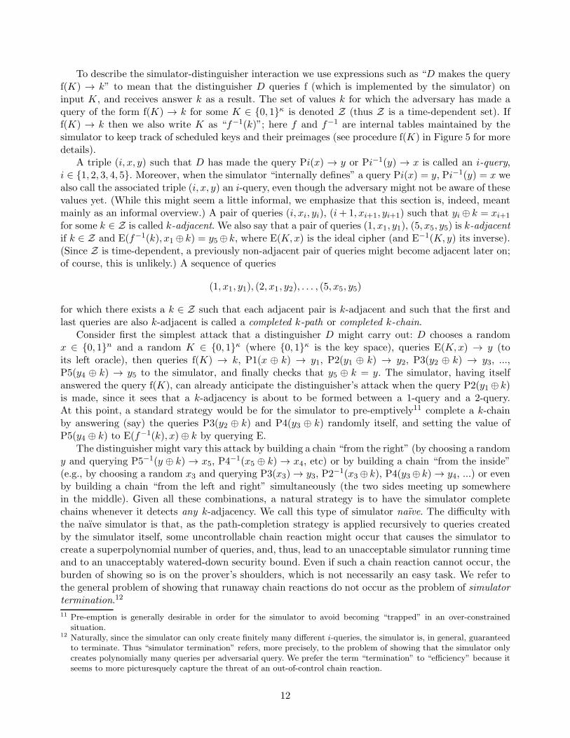
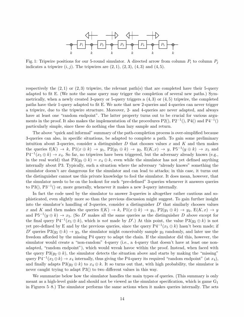
(and no tripwires of the form (1, 5) or (5, 1)), as sketched in Figure 1. This simulator has the advan-tage of having a clean (though combinatorially demanding) termination argument, and, as previouslydiscussed, of having excellent efficiency and also better security than the state-of-the-art in “indiffer-entiable blockcipher” constructions.

Some more high-level description of the 5-round simulator. We have already mentionedthat our 5-round simulator has tripwires

(2, 1), (2, 3), (4, 3), (4, 5).

To complete the simulator’s description it (mainly) remains to describe how the simulator completeschains, once a tripwire is triggered, since there is some degree of freedom as to which i-query is“adapted” to fit E, etc. Quickly and informally, when a newly created 1-query or 3-query triggers

13

k k k k k k

P1 P2 P3 P4 P5

Fig. 1: Tripwire positions for our 5-round simulator. A directed arrow from column Pi to column Pj

indicates a tripwire (i, j). The tripwires are (2, 1), (2, 3), (4, 3) and (4, 5).

respectively the (2, 1) or (2, 3) tripwire, the relevant path(s) that are completed have their 5-queryadapted to fit E. (We note the same query may trigger the completion of several new paths.) Sym-metrically, when a newly created 3-query or 5-query triggers a (4, 3) or (4, 5) tripwire, the completedpaths have their 1-query adapted to fit E. We note that new 2-queries and 4-queries can never triggera tripwire, due to the tripwire structure. Moreover, 2- and 4-queries are never adapted, and alwayshave at least one “random endpoint”. The latter property turns out to be crucial for various argu-ments in the proof. It also makes the implementation of the procedures P2(), P2−1(), P4() and P4−1()particularly simple, since these do nothing else than lazy sample and return.

The above “quick and informal” summary of the path-completion process is over-simplified because3-queries can also, in specific situations, be adapted to complete a path. To gain some preliminaryintuition about 3-queries, consider a distinguisher D that chooses values x and K and then makesthe queries f(K) → k, P1(x ⊕ k) → y1, P2(y1 ⊕ k) → y2, E(K,x) → y, P5−1(y ⊕ k) → x5 andP4−1(x5 ⊕ k) → x4. So far, no tripwires have been triggered, but the adversary already knows (e.g.,in the real world) that P3(y2 ⊕ k) = x4 ⊕ k, even while the simulator has not yet defined anythinginternally about P3. Typically, such a situation where the adversary “already knows” something thesimulator doesn’t are dangerous for the simulator and can lead to attacks; in this case, it turns outthe distinguisher cannot use this private knowledge to fool the simulator. It does mean, however, thatthe simulator needs to be on the lookout for such “pre-defined” 3-queries whenever it answers queriesto P3(), P3−1() or, more generally, whenever it makes a new 3-query internally.

In fact the code used by the simulator to answer 3-queries is altogether rather cautious and so-phisticated, even slightly more so than the previous discussion might suggest. To gain further insightinto the simulator’s handling of 3-queries, consider a distinguisher D′ that similarly chooses valuesx and K and then makes the queries f(K) → k, P1(x ⊕ k) → y1, P2(y1 ⊕ k) → y2, E(K,x) → yand P5−1(y ⊕ k) → x5. (So D′ makes all the same queries as the distinguisher D above except forthe final query P4−1(x5 ⊕ k), which is not made by D′.) At this point, the value P3(y2 ⊕ k) is notyet pre-defined by E and by the previous queries, since the query P4−1(x5 ⊕ k) hasn’t been made; ifD′ queries P3(y2 ⊕ k) → y3, the simulator might conceivably sample y3 randomly, and later use thefreedom afforded by the missing P4 query to adapt the chain. If the simulator did this, however, thesimulator would create a “non-random” 4-query (i.e., a 4-query that doesn’t have at least one non-adapted, “random endpoint”), which would wreak havoc within the proof. Instead, when faced withthe query P3(y2 ⊕ k), the simulator detects the situation above and starts by making the “missing”query P4−1(x5⊕ k)→ x4 internally, thus giving the P4-query its required “random endpoint” (at x4),and finally adapts P3(y2 ⊕ k) to x4 ⊕ k. It so turns out that, with high probability, the simulator isnever caught trying to adapt P3() to two different values in this way.

We summarize below how the simulator handles the main types of queries. (This summary is onlymeant as a high-level guide and should not be viewed as the simulator specification, which is game G1

in Figures 5–8.) The simulator performs the same actions when it makes queries internally. The sets

14

LeftQueue and RightQueue mentioned below are two queues of queries maintained by the simulatorfor the purpose of tripwire detection. When a new i-query is created, i ∈ {1, 3}, that the simulatorbelieves might set off the (2, 1) or (2, 3) tripwire, the simulator puts this i-query into LeftQueue, to bechecked later; similarly for i ∈ {3, 5}, the simulator puts a newly created i-query into RightQueue ifit believes this new query might set off a (4, 3) or (4, 5) tripwire. (The same 3-query might end up inboth LeftQueue and RightQueue.) As evidenced by the procedure EmptyQueue() in Fig. 7, LeftQueueand RightQueue are emptied sequentially and separately, which we choose to do mostly because itoffers conceptual advantages within the proof.

The simulator in pseudocode. The global variables present in game G1 are tables P1, P−11 , P2,

P−12 , . . . , P5, P

−15 as well as a table ETable[K] for each K ∈ {0, 1}κ, the (partially defined) keying

function f and its inverse f−1, the set of subkeys Z (being the image of f), the FIFO queues LeftQueueand RightQueue, the sets LeftFreezer and RightFreezer, as well as “bookkeeping sets” Queries andKeyQueries that we discuss below (the set EQueries is only used in game G2). Finally, there aretwo global variables qnum and Eqnum; these are “query counters” (initially set to 0) that measure,respectively, the size of the set Queries and the number of distinct queries to E or E−1 made internallyby the simulator; for the purpose of counting the latter, an additional table TallyETable, similar toETable, is used by the function TallyEQuery (Figure 8). All global variables are persistent, in thesense that they maintain their state from one distinguisher query to the next. By kZ, we denote thek-fold direct sum Z ⊕ · · · ⊕ Z of Z.

The tables P1, P−11 , P2, P

−12 , . . . , P5, P

−15 are maintained by the simulator and correspond to the

five permutations. Here P1(x) = y, P−11 (y) = x if x maps to y under the first permutation, etc; initially,

every entry in every Pi is ⊥, and the simulator fills in entries as the game progresses. Consistencybetween Pi and P−1

i is always maintained: we have Pi(x) = y if and only if P−1i (y) = x, for all x, y ∈

{0, 1}n; moreover, entries are never overwritten. We let domain(Pi) = {x : Pi(x) 6= ⊥}, range(Pi) ={y : P−1

i (y) 6= ⊥}. Each pair of tables ETable[K], ETable[K]−1 is similarly maintained by the idealcipher E.

Our simulator can abort (“abort”). When the simulator aborts, we assume that the distinguisherD is consequently notified, and that D can then return its own output bit. (Since the “real world”never aborts, there should be little doubt about D’s opinion, in this case, but D can return as itwants.)

Importantly, the simulator and the cipher E take explicit random tapes as randomness sources.The simulator’s random tapes are tables p1, . . . , p5 and rf . Here pi is actually two tables pi(→, ·) andpi(←, ·) defining a uniform random permutation; i.e., for every x, y ∈ {0, 1}n we have pi(→, x) = yif and only if pi(←, y) = x, and pi is selected uniformly at random from all pairs of tables pi(→, ·),pi(←, ·) with this property. Likewise, the random tape pE for E’s use consists of a different randompermutation pE[K] for each K ∈ {0, 1}κ encoded as two tables pE[K](→, ·), pE [K](←, ·). The table rfsimply holds uniform random n-bit values: rf (K) is uniform at random in {0, 1}n for each K ∈ {0, 1}κ.

The simulator uses the table pi when it wants to “lazy sample”, say, Pi(x); instead of doing the

random sampling on its own by a call such as “Pi(x)$← {0, 1}n\range(Pi)”, the simulator will call

the function ReadTape(Pi, x, pi(→, ·)). (Concerning the implementation of ReadTape: we assume that(P−1

i )−1 = Pi, etc.) If all of the previously defined entries in Pi have been sampled via calls to

ReadTape, the effect of calling ReadTape is identical to the instruction Pi(x)$← {0, 1}n\range(Pi),

i.e., the outcomes are identically distributed. But if some entries of Pi have been adapted (i.e., not setvia lazy sampling), then ReadTape might abort if, through bad luck, it hits an adapted value. Hencethe use of ReadTape is not quite equivalent to pure lazy sampling, though the difference is fairly slight.Moreover, this issue does not arise when E uses ReadTape, because E never adapts its queries. (Inthe previous discussion we omitted mentioning ReadTape and the use of “explicit randomness” by the

15

simulator, and we pretended that the simulator did pure lazy sampling; this is not quite the case, butit matters little for that discussion.)

We also note that while the random tapes represent an “unreasonably large” amount of at-handrandomness, the simulator (and ideal cipher E) can simulate access to such random tapes via lazysampling. For example, the simulator just keeps a partially defined copy of pi “in its head” for whichit does (true) lazy sampling whenever it needs to read a new entry. Hence, access to this type ofrandomness can also be efficiently simulated, and we are not “cheating” by giving the simulator accessto such random tapes.

Whenever the simulator defines a new entry in Pi it creates a “bookkeeping record” of this newentry in the set Queries. More precisely, a new entry Pi(x) = y, P−1

i (y) = x is recorded as a tuple(i, x, y, dir, num) added to the set Queries, where dir ∈ {←,→,⊥} is the “direction” of the query andwhere num is the previous value of qnum, incremented by one (we call this the “query number” of thenew tuple). Here dir = → if the new Pi entry is created by a call of the type ReadTape(Pi, x, pi(→, )),and dir = ← if it is created by a call of the type ReadTape(P−1

i , y, pi(←, ·)). In all other cases,dir = ⊥. Queries with dir = ⊥ are called adapted. The set KeyQueries is similarly maintained, but issimpler (see the function ‘AddKeyQuery’ in Figure 8). We note that KeyQueries and Queries bothshare the same “query counter” qnum, so that elements of these lists are totally ordered by their lastcoordinates.

We sometimes omit the last coordinate or last two coordinates of a query (i, x, y, dir, num)—writingsimply (i, x, y, dir) or (i, x, y)—when these coordinates aren’t of interest to the discussion at hand.

4.2 Proof Techniques

A self-contained overview of the indifferentiability proof appears in Section 4.3. Here we mention onlythe “main highlights”(with emphasis on novelties).

Our indifferentiability proof uses a fairly short sequence of games, with only four games in all. Thefirst game implements the “simulated world” while the last game implements the “real world”. A novelfeature of our proof is that we use no “bad events” to bound the distinguishability of adjacent games.In places where a “bad event” flag might traditionally be used, our code simply aborts instead.

In a little more detail, the second game is identical to the first game except that it containseven more abort conditions than the first game. (Some of these new abort conditions involve thesimulator “illegally” examining queries made by the adversary to the ideal cipher, which is why theseabort conditions cannot be incorporated in the original simulated world.) Since the fourth game neveraborts, and since the second game is identical to the first except that it sometimes aborts when thefirst game doesn’t, it suffices to upper bound the distinguishability of the second and fourth games.

The third game changes only the implementation of the ideal cipher, which is no longer “ideal” inthe third game, but is indeed implemented as a key-alternating cipher, where the key-alternating cipheruses the same random tapes (i.e., permutations and key scheduling function) as the simulator uses. Thetransition from the second to third game is the crucial transition, and to be perfectly formal we usethe nice “randomness mapping” technique of Holenstein et al. [37]. This technique links the executionsof two games with explicitly given random coins by exhibiting a partial bijective function from the setof random tapes in one game to the set of random tapes in the other that preserves game behavior,as viewed by the distinguisher. Our randomness mapping argument presents some novelties, however.In particular, we observe that it is sufficient for executions that are paired up by the randomness map(one execution in the second game, one execution in the third game) to have very similar probabilitiesof occurring in each world as opposed to exactly equal probabilities of occurring. This natural relaxationallows us to handle lazy permutation sampling without the complicated workarounds of Holenstein etal. (in particular without use of a “two-sided random function”) and considerably simplifies the whole

16

argument. Our randomness mapping argument also introduces the idea of random footprints and ofexecution trees, of potential independent interest.

The transition from the third game to the fourth game is rather straightforward, as one can show(somewhat similarly to the first and second games) that the third and fourth games proceed identicallyon identical random tapes except for the possibility that the third game might abort while the fourthgame (which is the real world) never aborts. For this transition it thus suffices to upper bound theprobability of the third game aborting, which is easy to do once we have already proved that thesecond game aborts with small probability (establishing the latter is necessary for the randomnessmapping argument) and by the previously established similarity of the second and third games.

Another “syntactic novelty” in our proof, besides the fact that we eschew bad events in favor ofabort conditions, is that our simulator maintains explicit “bookkeeping” data structures in additionto its other data structures. The bookkeeping data structures keep track, among others, of the orderand “direction” (for permutation queries) of queries internally defined by the simulator. There aretwo main advantages here: (1) having an unambiguous timeline and description of events withinthe data structures themselves, which clarifies arguments within the proof; (2) the fact that the“bookkeeping copy” is only updated with new information after a series of checks have been made (ifone of these checks isn’t passed, the simulator aborts) which implies that various “good invariants”(postulated about the bookkeeping data structures instead of about the primary data structures)can be shown to hold unconditionally at any point in any execution. Having such “unconditionalinvariants” considerably simplifies the language in the proof, which is a very non-negligible gain. Onecould theoretically achieve the same effect using only primary data structures, but then one cannot,for example, include an instruction that simultaneously reads from a random tape and updates theprimary data structure with the read value, since the value might momentarily corrupt an invariant(even if this is caught and abort occurs soon after, the invariant no longer holds unconditionally atall points in time). One would need, instead, to check the value after reading it from the random tapebefore using it. By contrast, being able to immediately use a random value and then check its goodnessonly a few lines later, when it comes time to update the bookkeeping data structure, produces muchmore readable code.

Another standard concern of indifferentiability proofs is the issue of simulator termination, alreadymentioned in the previous subsection. For more details on the termination argument we refer to theoutline in Section 4.3 (the termination argument itself appears in Appendix C).

4.3 Proof Overview

In this section we give the backbone of the proof of Theorem 3, our main result: the indifferentiabilityof 5-round key-alternating cipher with RO-scheduled subkeys. Some supporting lemmas are found inAppendices C and D.

The simulator S referred to in the statement of Theorem 3 is, of course, the simulator outlined inSection 4.1, and formally given by the game G1 in Figures 5–8.

We start by noting that Theorem 3 actually consists of three separate claims: (i) the indistin-guishability of the real key-alternating cipher and of its simulated counterpart; (ii) the fact that Snever makes more than 2q2 queries to the ideal cipher IC (renamed as the functions E, E−1 in gameG1) when interacting with a q-query distinguisher D; (iii) the fact that that S’s total running time13

is O(q3) with probability 1. Proofs of (ii) and (iii) can be found in lemmas 9 and 10 at the end of thesection. The rest of our discussion is devoted to (i).

13 For simplicity, every pseudocode instruction is assumed to take unit time. Other models of running time mightintroduce additional factors of order O(n).

17

Our indistinguishability argument uses a sequence of four games. Each game is an environment inwhich the distinguisher D can be run. We start by briefly describing the four games:

• Game G1 (Figures 5–8 in Appendix B) is “the simulated world”. The distinguisher’s left oracleE, E−1 implements an ideal cipher, while the distinguisher’s right oracle, consisting of eleven distinctinterfaces f, P1, P1−1, . . ., P5, P5−1 implements our 5-round simulator as discussed in Section 4.1.

• Game G2 (Figures 5–8 in Appendix B) makes some modest changes to game G1. Essentially, anumber of abort conditions are added to the simulator, and some abort conditions are also added toE/E−1. G2 uses the same random tapes as G1, and two executions of G1 and G2, for the same randomtapes and the same distinguisher queries, will proceed identically except for the possibility that G2

might abort when G1 does not. We note that one of the abort conditions added to the simulator ingame G2 (in the function FreezeLeftValues(), Figure 6) “illegally” examines the private tables ETable[·]maintained by the cipher E, and also that E now examines the simulator’s own tables from within thefunction AddEQuery; however, since this is an intermediate game and not the simulated world, theseidiosyncrasies are of no import.

• Game G3 (Figure 9 in Appendix B) changes the procedures E(K, ·), E−1(K, ·) to directly use thetable rf (in order to compute the key schedule k ofK) and the permutation tables p1, . . . , p5 to computeits answers, treating these tables as the cipher’s underlying permutations. Moreover, a second (shallow)change occurs in game G3, in that the random tables p1, . . . , p5 are actually renamed as q1, . . . , q5,in order to facilitate future comparison between games G2 and G3. However, the simulator-relatedprocedures of game G3 are not rewritten to reflect this change, since this would more or less be awaste of paper. To summarize: game G3 is obtained by changing pi everywhere to qi in game G2, andby replacing the procedures E and E−1 of Figure 5 with those of Figure 9.

• Game G4 (Figure 9 in Appendix B) is the “real world”: the simulator directly answers queriesusing rf and the permutation tables q1, . . . , q5, while E/E−1 are unchanged from game G3.

Proving indifferentiability amounts to showing that games G1 and G4 are indistinguishable. Forthis, it turns out to be helpful if we first “normalize” the distinguisher D. More precisely, we assume(i) that D is deterministic and always outputs either 1 or 0, (ii) that D outputs 1 if the system aborts,and (iii) that D completes all paths, meaning that for every query E(K,x) → y or E−1(K, y) → xmade by D, D eventually makes the (possibly redundant queries)

f(K)→ k, P1(x⊕ k)→ y1, P2(y1 ⊕ k)→ y2, . . ., P5(y4 ⊕ k)→ . . .

in this order, unless it is prevented from doing so because the system has aborted. (Presumably, theoutput of the query P5(y4⊕k) will be y⊕k, but whether this is the case does not concern the definitionof a path-completing distinguisher.) Points (i) and (ii) are obviously without loss of generality, sinceG4 never aborts. Point (iii) is also without loss of generality as long as we give D a few extra queries(or, to be precise, a factor 6 more queries), since D is free to ignore the information that it gatherswhile path-completing. In more detail, we first prove indifferentiability with respect to a “normalized”(i.e., deterministic, path-completing, etc) q-query distinguisher D, and then deduce our main theoremvia a straightforward reduction (with a factor 6 loss in the number of queries).

Thus let D denote a fixed, q-query deterministic distinguisherD that completes all paths. Notationssuch as

DG2 = 1 and DG2(α) = 1

indicate that D outputs 1 after interacting with G2, but the second notation explicitly mentions therandom tape α = (rf , p1, . . . , p5, pE) on which the game is run. It is sufficient and necessary to upperbound

Pr[DG1 = 1]− Pr[DG4 = 1]

18

where the probabilities are computed over the explicit random tapes in each game (and only over theserandom tapes, since D is deterministic). Since game G2 only introduces additional abort conditionsfrom G1 and since D outputs 1 when the game aborts, we have

Pr[DG2 = 1] ≥ Pr[DG1 = 1]

and so it suffices to upper bound

Pr[DG2 = 1]− Pr[DG4 = 1].

For the latter, we apply a standard hybrid argument by upper bounding

Pr[DG2 = 1]− Pr[DG3 = 1] (3)

andPr[DG3 = 1]− Pr[DG4 = 1] (4)

separately.The crux of the proof to upper bound (3), i.e., the game transition from G2 to G3, as the transition

from G3 to G4 turns out to be much less problematic (cf. Lemma 8 below). To upper bound thetransition from G2 to G3 we essentially use a randomness mapping argument a la Holenstein etal. [37]. It seems worthwhile to first give a high-level overview of the randomness mapping argument,which requires a few more definitions.

Randomness mapping (high-level overview). An execution consists of the start-to-finish inter-action of D with either G2 or G3, including all internal actions performed by the simulator (i.e.,performed by the game14). Since D is fixed and deterministic, we note that every tuple of randomtapes in G2 determines a unique G2-execution and likewise every tuple of random tapes in G3 de-termines a unique G3-execution. On the other hand, two different tuples of (say) G2 random tapesmight give rise to the same G2 execution since certain portions of the random tapes might not be read,and thus not affect the execution. (The execution includes everything read from the random tapesbut not the random tapes themselves.) If α = (rf , p1, . . . , p5, pE) is a G2 random tuple, the footprintof α consists of that portion of the random tapes actually read during the execution DG2(α). (Thissomewhat hand-wavy definition is more carefully restated below.) We make a similar definition forG3. By definition, then, there is a bijection between the set of possible G2 executions and the set ofdifferent G2 footprints, and similarly there is a bijection between the set of possible G3 executionsand the set of different G3 footprints. We say a G2 footprint is good if G2 does not abort on thatexecution, and likewise a G3 footprint is good if G3 does not abort on the corresponding execution.

One can observe that not all footprints have the same probability of occurring, even ifD is somehownormalized to always make the same number of queries (which we are not even assuming); for example,if D only makes queries to the key scheduling function f on a certain execution, that execution’sprobability will be a power of (1/2n), which will not be the case for a generic execution.

In a nutshell, the randomness mapping argument upper bounds Pr[DG2 = 1] − Pr[DG3 = 1] byexhibiting a bijection τ between the set of good G2 footprints and good G3 footprints such that (i) τpreserves the output of D (indeed, τ maps G2 executions to G3 executions that look exactly the samefrom D’s viewpoint); (ii) τ maps executions of G2 to executions of G3 of nearly equal probability. Forthe randomness mapping to be effective, one obviously needs, thirdly, the set of good G2 footprints torepresent most of the probability mass of all G2 footprints (since the domain of τ is limited to good

14 In G2 and G3 we use “simulator” and “game” interchangeably. This choice of terminology would make less sense forG1, since the functions E/E−1 are obviously not part of the “original” simulator.

19

footprints), which is exactly the same as saying that one needs the probability of abortion to be lowin G2. One of the main sub-goals of the proof, thus, is to show that G2 aborts with low probability.

We note that our randomness mapping argument has some significant differences with that ofHolenstein et al., from a technical standpoint. Most notably, Holenstein et al.’s randomness map hasthe property that an execution and its image under the map have exactly the same probability insteadof nearly equal probability. To achieve this Holenstein et al. need, in particular, to use random tapesin which each n-bit block is uniformly random and independent from other n-bit blocks in the tape.Such a random tape cannot represent a random permutation which means that Holenstein et al.have to jump through various hoops in order to work with random permutations, thus significantlycomplicating their proof. We believe that relaxing the requirements on the randomness map constitutesa more efficient and natural approach. A second difference is that Holenstein et al. reason directlyabout the “original” probability space consisting of all possible random tapes instead of reasoningabout the “induced” probability space consisting of all possible footprints (which we found to be moreconvenient).

On the other hand, the idea of working with a distinguisher D that completes all paths is lifteddirectly from [37]. Without such a distinguisher, defining the randomness map seems much harder.(Indeed, finding a clean-cut proof that does not require a distinguisher that completes all paths wouldbe a significant technical innovation for such proofs.)

G2 abortion and termination argument. As noted in the outline above, proving that G2 abortswith small probability is a central component of the proof. The following lemma, which upper boundsthis probability, is proved in Appendix C:

Lemma 1. The probability of abortion is at most 160q10/2n in G2. I.e.,

Pr[(rf , p1, . . . , p5, pE) are good for G2] ≥ 1−160q10

2n

for any (q-query, deterministic) distinguisher D.

Because G2 automatically aborts if the simulator makes too many internal queries (see the functionAddQuery in Fig. 7) proving Lemma 1 subsumes the termination issue, i.e., to prove Lemma 1 we inparticular need to prove that “out-of-control” chain reactions either don’t occur or else occur with lowprobability in game G2. (While proving out-of-control chain reactions occur only with low probabilitywould be sufficient, we show in Appendix C that such chain reactions don’t occur at all. Indeed, G2

pre-emptively aborts when any anomalies occur that might eventually lead to such reactions.) Whiletermination is thus the domain of Lemma 1 and of Appendix C we include a (very) high-level outlineof the termination argument here for the curious reader’s sake. We can emphasize at the outset thatour termination argument bears no relation at all to Holenstein et al.’s, as our termination argumentrelies on fine-grained combinatorial observations that are tailored to our simulator and to the settingof key-alternating ciphers.

Let us first recall how a (not out-of-control) “chain reaction” might occur in the first place. Saya distinguisher D makes the queries f(K1) → k1, f(K2) → k2, f(K3) → k3, f(K4) → k4, then choosesa value x12 ∈ {0, 1}

n and makes the queries P2(x12) → y12, P2−1(y22) → x22 where y22 := y12 ⊕ k1 ⊕ k2,

P2(x32) → y32 where x32 := x22 ⊕ k2 ⊕ k3, P2−1(y42) → x42 where y42 := y32 ⊕ k3 ⊕ k2. Let y11 := x12 ⊕ k1,

x123 := y12 ⊕ k1 = y22 ⊕ k2, y231 := x22 ⊕ k2 = x32 ⊕ k3, x

343 := y32 ⊕ k3 = y42 ⊕ k4 and y41 := x42 ⊕ k4. If

the distinguisher queries P1−1(y11) at this point the simulator will create a new 1-query (1, x11, y11,←)

and put this query on LeftQueue; the query is immediately popped from LeftQueue, and the simulatordetects that y11 is k1-adjacent to the pre-existing 2-query (2, x12, y

12 ,→), so the simulator completes a

path of subkey k1 passing through the points y11 and x123 , and in particular creates a new 3-query

20

(3, x123 , y123 ,→) in the process that is put on LeftQueue (in the form of the pair (3−, x123 )); when this 3-query is popped from LeftQueue, a k2-adjacency with the pre-existing 2-query (2, x22, y

22) is uncovered,

leading to the completion of a path of label k2 going through y231 , and so on. In all, the simulatorcreates paths of labels k1, k2, k3 and k4 before LeftQueue is finally emptied.

In our proof, the 2-queries (2, x12, y12), . . ., (2, x

42, y

42) together with the scheduled keys k1, . . . , k4 ∈ Z

gives rise to a connected component of 4 edges in a bipartite graph called B2. (In fact, the way B2 isdefined, the edges have endpoints y11, x

123 , y231 , x343 , y41 and are labeled by the values k1, . . . , k4. Each

2-query gives rise to |Z| different parallel edges of B2.) A similar graph B4 is defined with respectto 4-queries. Essentially, the graphs B2 and B4 are defined such that chain reactions occur withinconnected components of B2 and B4, as in the case above with B2.

The key observation we make is that while a chain reaction is “burning through” a connectedcomponent of B2, no edges are added to B2 (thus not enlarging the size of the maximum connectedcomponent of B2) while the edges that are added to B4 are disconnected15 from previous connectedcomponents of B4 by design; for example, when the new 3-query (3, x123 , y123 ,→) is created above, theset of values y123 ⊕ 4Z is disjoint from the set of left endpoints of edges in B4 with high probabilitybecause the query has direction → (and if it isn’t disjoint the simulator actually aborts; cf. the first“forall” loop of procedure QueryChecks in Fig. 8). In a nutshell, the modifications made to B4 whilea component of B2 is being processed are “random and therefore harmless”, and vice-versa.

To be a little more precise we succeed in showing that the size of the largest maximum connectedcomponent (of a certain “unprocessed” type) in the disjoint union of B2 and B4 grows by at most 2every time the simulator answers an adversarial query. Thus the size of the largest component in B2,B4 grows no faster than linearly in the number of queries, which cinches the termination argument.

Of course, the termination argument is not quite as simple as sketched above. In particular, thefour-query example that we used doesn’t represent the full complexity of cases that can occur. E.g.,the distinguisher might first make a 3-query and then build large connected components in both B2

and B4 on either side of this 3-query without triggering any tripwires before “lighting the fuse” andcausing the components on both sides to be processed. Or the adversary might make matching 1- and5-queries (i.e., via an E-query), attach a B2 component to the 1-query and a B4 component to the5-query without triggering any tripwires, and then cause both these components to be processed bymaking a single query. All possible cases are analyzed in Appendix C, and we refer in particular tothe proof of Lemma 18 for a detailed and leisurely walkthrough. A salient and important feature ofall cases, however, is that at most one pre-existing component of B2 and one pre-existing componentof B4 is affected per distinguisher query.

The transition from G2 to G3, and the rest of the proof. Having given outlines of theproof’s main elements above (randomness mapping and termination) we continue with more details,in particular upper bounding the transition from G2 to G3 and the transition from G3 to G4. Weassume Lemma 1 which is proved in Appendix C.

A tuple of random coins(rf , p1, . . . , p5, pE)

for G2 is called a G2-tuple, whereas a tuple of random coins

(rf , q1, . . . , q5)

for G3 is, likewise, called a G3-tuple. We let R2 be the set of all G2-tuples, and R3 be the set of allG3-tuples. Elements in R2 ∪R3 are simply called random tuples.

15 This oversimplifies. In specific situations one or two edges may be added to unprocessed components of B4. SeeAppendix C for more details.

21

We say a G2-tuple

(rf , p1, . . . , p5, pE) ∈ R2

is good (with respect to our fixed distinguisher D) if the simulator doesn’t abort for this tuple. In this

case, we also say that the interaction of D with G2 constitutes a good execution. We let Rgood2 ⊆ R2

be the set of all good G2-tuples. We emphasize that Rgood2 depends on D, even if this dependency is

not reflected in the notation.

We can view the permutation tables p1, . . . , p5, {pE [K] : K ∈ {0, 1}κ}, q1, . . . , q5 that are presentin random tuples as perfect matchings from {0, 1}n to {0, 1}n. The restriction of such a matching(permutation) p is obtained by removing a subset of the edges (possibly empty); this can still beencoded as a table p by setting relevant entries p(→, x) and p(←, y) to ⊥. Likewise, a restriction of rfis obtained by setting certain entries of rf to ⊥. Finally, the restriction of a G2-tuple (rf , p1, . . . , p5, pE)is obtained by taking arbitrary restrictions of each coordinate (for pE, we mean taking a differentrestriction of pE [K] for each K ∈ {0, 1}κ). We call the result a partial G2-tuple or a restricted G2-

tuple. We let Rpartial2 be the set of all partial G2-tuples, and we define Rpartial

3 similarly. (In particular,

Rj ⊆ Rpartialj for j = 2, 3.)

Running G2 on an element of Rpartial2 doesn’t necessarily make sense, since G2 might access a ⊥-

value. But if G2 doesn’t access any such entries, then the execution, obviously, is well-defined. Similarremarks hold for G3 and for Rpartial

3 .

We say an edge (x, y) of a permutation p of a random tuple is examined during an execution of therelevant game (either G2 or G3, and for our fixed distinguisher D) if the value p(→, x) or p(←, y) isever read; likewise we say an entry rf (x) is examined during an execution, if it is read. The footprint ofa random tuple is the partial tuple obtained by keeping only the edges examined during the executionassociated to that tuple, and by likewise keeping only the entries of rf examined during that tuple.

Thus a footprint for G2 is an element of Rpartial2 , and a footprint for G3 is an element of Rpartial

3 .

Since the only source of randomness is the coins (rf , p1, . . . , p5, pE) in G2 and (rf , q1, . . . , q5) in G3,we note that an execution’s footprint contains all the information necessary to re-create the execution.Thus, there is a bijective correspondence between the set of possible executions and the set of possiblefootprints. (Still, always, for our fixed D.)

We let Rfootj ⊆ Rpartial

j denote the set of Gj-footprints and let Rgood-fj ⊆ Rfoot

j be the set footprints

of good executions in Gj for j = 2, 3. (Note that Rgood-fj 6⊆ Rgood

j due to the fact that Rgood-fj contains

partial tuples, whereas Rgoodj , by definition, contains full tuples.)

The execution tree of a game (say G2) groups all possible executions with distinguisher D asfollows: each time a value is read from one of the random tables (rf , p1, . . . , p5, pE), the tree forks intoas many branches as there are possible answers. (So for example, when a value is read from rf , thiscorresponds to a 2n-wise fork; if a value is read from p1 (in either direction) when two values havealready been read from p1, this gives rise to a (2n−2)-wise fork in the execution tree, and so on.)The leaves of the tree correspond to aborted states or to points at which D decides to return. (Sincein any case D returns 1 after abortion, all leaves, in effect, correspond to return points of D.) Welabel the leaves by the return value of D. (We emphasize that the nodes in the execution tree do notcorrespond to queries made by D; every node in the execution tree corresponds, instead, to randomtape accesses. Indeed, with D being deterministic, these accesses are the only “source of branching”when D interacts with G2.) The execution tree of G3 is defined similarly.

The possible executions of G2 are in bijective correspondence with the leaves in the executiontree of G2 (ditto for G3), and, by the same token, in bijective correspondence with the differentpossible footprints for G2 (ditto for G3). Moreover, the probability that a leaf v is reached (withprobability taken over the uniform choice of (rf , . . . , pE) ∈ R2 in G2 and over the uniform choice of

22

(rf , . . . , q5) ∈ R3 in G3) is∏

u

1

deg(u)

where the product is taken over all nodes u from the root of the tree to v, and where deg(u) is thedegree of u (as is easy to see). We also note that the depth of a leaf v (i.e., the path length from vto the root) is the total number of permutation edges plus the number of rf -entries in the footprintassociated to v.

We also note that the probability of a leaf can be easily computed from the leaf’s footprint,without having to retrace the execution associated to the footprint. More precisely, if we notate by|p| the number of edges in a partial matching p and if we notate by |rf | the number of non-⊥ entries

in rf , then the probability of reaching a leaf v with footprint (rf , p1, . . . , p5, pE) ∈ Rpartial2 in the G2

execution tree is(

1

2n

)|rf |(

5∏

i=1

(2n − |pi|)!

2n!

)

∏

K∈{0,1}κ

(2n − |pE [K]|)!

2n!

.

A similar (but simpler) computation holds for leaves of G3.

Let PrG2[v] denote the probability of reaching a leaf v of the G2 execution tree, and likewise define

PrG3[v] to be the probability of reaching a leaf v in the G3 execution tree. Let lf1(G2) be the set of

1-leaves in the G2 execution tree, and likewise for G3. Then

Pr[DG2 = 1] =∑

v∈lf1(G2)

PrG2[v]

and a similar equation holds for G3.

As already outlined, the basic idea of the randomness mapping argument is to exhibit an injectivemapping τ from the leaves of the G2 execution tree to the leaves of the G3 execution tree such that(i) the domain of τ is all (leaves associated to) non-aborted G2 executions (and, in particular, “almostall” leaves are in the domain of τ , as measured by their total probability mass), (ii) τ maps 1-leaves to1-leaves and 0-leaves to 0-leaves, and (iii) PrG2

[v] is very close to PrG3[τ(v)], for all v in the domain

of τ . Details follow.

We start by defining a map

τ : Rgood2 → Rpartial

3 .

In a second step, we will show that the “restriction” of τ to the footprint of a G2-tuple (rf , . . . , pE)makes sense (so that τ can be defined on the non-aborted leaves of the G2 execution tree, i.e., can be

defined on Rgood-f2 ), and that elements in the image of τ are in fact in Rgood-f

3 , so that the range of τconsists of leaves of the G3 execution tree.

Let α := (rf , p1, . . . , p5, pE) ∈ R2. Then τ(α) is simply defined according to the tuple (f, P1, . . .,P5), as it stands at the end of the execution ofDG2 with randomness α. More precisely, if (r∗f , q1, . . . , q5)is the image of τ(α), then r∗f (K) = f(K) for all K ∈ {0, 1}κ, qi(→, x) = Pi(x) for all x ∈ {0, 1}

n, and

qi(←, y) = P−1i (y) for all y ∈ {0, 1}n. (In this case, we also say that qi is a copy of Pi.) Clearly, τ(β)

is also well-defined for any footprint β, and in particular for any β ∈ Rgood-f2 .

The next proposition (variants of which are also proved in Appendix C) makes a few basic obser-vations that are helpful, in particular, for the subsequent lemma.

Proposition 1. Consider a non-aborting execution of G2. Let (j, x, y, dir, num) be a query (i.e., anelement of Queries) with j = 2 or j = 4. Then dir ∈ {←,→}. Moreover, if (i, xi, yi, diri, numi),

23

(i + 1, xi+1, yi+1, diri+1, numi+1) are k-adjacent queries for some k ∈ Z, with (K, k, numk) the cor-responding element of KeyQueries, then (i) numk < max(numi, numi+1), and (ii) diri =→ impliesnumi < numi+1 whereas diri+1 =← implies numi > numi+1.

Proof. The first assertion is a consequence of the fact that 2-queries and 4-queries are always lazy-sampled (see the code of the procedures P2() and P4()). Point (i) of the second assertion is a directconsequence of the abort condition in the second for-loop of the procedure KeyQueryChecks in Figure8 while point (ii) is a direct consequence of point (i) and of the checks that occur in the first twofor-loops of the procedure QueryChecks (still Figure 8), since Z ⊆ 5Z. ⊓⊔

Lemma 2. Assume that D is a distinguisher that completes all chains, and let P1, . . . , P5, Queries,EQueries and f be the global variables in G2 at the end of a non-aborting (i.e., “good”) executionDG2 . Then for all (K,x, y) ∈ EQueries we have f(K) 6= ⊥ and there exists a corresponding completedpath in Queries, i.e., there exists a 5-tuple

(1, x1, y1), (2, x2, y2), (3, x3, y3), (4, x4, y4), (5, x5, y5)

in Queries such that x1 = x⊕ f(K), y5 = y ⊕ f(K) and such that yi ⊕ f(K) = xi+1 for i = 1, 2, 3, 4.

Proof. Let (K,x, y, dir) ∈ EQueries at the end of the G2 execution (with dir ∈ {←,→}). Then eitherD queried E(K,x) or E−1(K, y) at some point, or else the simulator made one of these queries fromwithin EmptyQueue(), ForcedP3() or CompletedPath() (since these are the only functions in whichthe simulator queries E). If D queried E(K,x) or E−1(K, y), then since D completes all chains D alsoqueries f(K) at some point and there exist five queries

(1, x1, y1, dir1, num1), (2, x2, y2, dir2, num2), . . . , (5, x5, y5, dir5, num5)

in Queries such that x1 = k ⊕ x1 and such that yi ⊕ k = xi+1 for i ∈ {1, 2, 3, 4}. We next argue thaty5 ⊕ k = y.

To see this, note that dir2 ∈ {←,→} by Proposition 1. Say first that dir2 = ←. Then, again byProposition 1, we have that num1 > num2, that f(K) is scheduled before query num1 is created,and that dir1 6= →. When query num1 is created, therefore, it goes onto LeftQueue, and when itis popped from LeftQueue we already have f(K) ∈ Z and y1 ⊕ f(K) = x2 ∈ domain(P2); thesimulator will therefore complete a path, at this point, for the pair of adjacent queries (1, x1, y1),(2, x2, y2), with respect to the cipher key K; since the simulator aborts if it cannot complete thepath successfully (and since the simulator hasn’t aborted), the path must therefore consist of queriesnum1, . . . , num5 above (obviously, one can “uniquely follow” a path from left to right), and we musthave y5 ⊕ f(K) = ETable[K](x), i.e., y5 ⊕ f(K) = y. In the second case, if dir2 = →, then we cansimilarly argue that num3 > num2, that f(K) was scheduled before num3 was created, and thatdir3 6= ←, so that (3−, x3) was placed on LeftQueue when query num3 was created, and so thatwhen this pair is popped from LeftQueue the simulator detects the adjacency y2 ⊕ f(K) = x3, andcompletes a path for queries num2 and num3, which must be the path above.

Next, we consider the case when the simulator made either the query E(K,x) or E−1(K, y) (butthe distinguisher did not make such queries). If the simulator makes (say) the query E(K,x) inEmptyQueue(), then obviously there exists a corresponding completed path in Queries since the simu-lator is in the process of completing this path, and since the simulator doesn’t abort on this execution,by assumption. Now say the simulator makes the query E(K,x) or E−1(K, y) in ForcedP3(i, z)—say, with i = 3−, x3 := z. For this query to be made, there must (already) exist queries (1, x1, y1),(2, x2, y2) ∈ Queries such that x = x1 ⊕ f(K) and y1 ⊕ f(K) = x2, y2 ⊕ f(K) = x3, and f(K) must

24

already be scheduled. If ForcedP3 finds that E(K,x)⊕ f(K) ∈ range(P5) then it completes the corre-sponding path up to the 3-query (3, x3, y3) := (3, x3, x4 ⊕ f(K)), which is left for PrivateP3() to add(and thus complete the path). Otherwise, if E(K,x) ⊕ f(K) /∈ range(P5), then ForcedP3 returns ⊥,but PrivateP3() will add (3−, x3) to LeftQueue, and when this pair is subsequently popped from Left-Queue in EmptyQueue(), the corresponding path will be completed because f(K) is already scheduledand (2, x2, y2) is already in Queries. (Calls to ForcedP3(i, z) with i = 3+ are argued symmetrically.)Finally, for queries to E/E−1 made by the simulator in the function CompletedPath(), the argumentis clear, because CompletedPath() aborts unless the E/E−1 query matches the existing path. ⊓⊔

Lemma 3. τ : Rgood-f2 → Rpartial

3 is one-to-one, and the image under τ of a good G2-footprint is agood G3-footprint of equal label (0 or 1).

Proof. Let α = (rf , . . . , pE) ∈ Rgood-f2 and let β = τ(α) = (r′f , q1, . . . , q5) ∈ Rpartial

3 . Since α is a

footprint, the f -entries defined at the end of the execution DG2(α) are exactly the non-⊥ entries inrf . Hence, by definition of τ , r′f = rf and β = (rf , q1, . . . , q5) where q1, . . . , q5 are copies of the tables

P1, . . . , P5 at the end of the execution DG2(α).We consider parallel executions ofDG2(α) andDG3(β). We note that the only difference between G2

and G3, besides the renaming of the random tapes p1, . . . , p5 and q1, . . . , q5, lies in the implementationof the procedures E, E−1. Thus, when E and E−1 are treated as black boxes, the only differences thatmay arise in the parallel executions of DG2(α) and DG3(β) (if any) must be due to one of: (i) differentanswers returned by the “black boxes” E or E−1; (ii) differences in the tables p1, . . . , p5 and q1, . . . , q5(since rf is the same for α and β, and since pE is only used within E/E−1).

In particular, to show that the two parallel executions don’t “diverge”, it is sufficient to show: (a)that queries to E and E−1 are always answered identically in both executions, and (b) that wheneveran assignment of the type y := Pi(x)← pi(→, x), P−1

i (y)← x or of the type x := P−1i (y)← pi(←, y),

Pi(x) ← y occurs in G2, then we have qi(→, x) = pi(→, x) and (necessarily) qi(←, y) = pi(←, y) inG3. (Indeed, (b) is sufficient since such assignments are the only ways in which the tables p1, . . . , p5,q1, . . . , q5 are used in either game.)

We prove (a) and (b) by induction on the number of steps having occurred in the parallel execution,where calls to E and E−1 are treated in a black-box fashion in order to keep the number of stepscomparable. Firstly, (b) is clear, since values in Pi are never overwritten and since values in Pi transferover to qi by definition of τ . For (a), we note that Lemma 2 implies that at the end of the executionof DG2(α), there exists a unique 5-chain in P1, . . . , P5 for every (distinct16 query to E/E−1 made byD or by the simulator such that the 5-chain is consistent with the E/E−1-query. Since q1, . . . , q5 arethe copies of P1, . . . , P5 at the end of the execution DG2(α), this directly implies (by construction ofE in G3) that queries to E and E−1 in G3 are answered the same as in G2. Hence the two parallelexecutions DG2(α) and DG3(β) are identical when E and E−1 are treated as black boxes.

We next argue that β is the footprint of some good leaf in the G3 execution tree. By the abovethe simulator does not abort in DG3(β) (because α is good) so it suffices to argue that all edges ofq1, . . . , q5 and that all non-⊥ entries of rf are examined during the execution DG3(β). For rf this isclear, since all these entries are examined during the execution DG2(α). If an edge in qi correspondsto a non-adapted value of Pi, i.e. to a value of Pi “downloaded” from pi, then this qi-edge is clearlyexamined during the execution DG3(β), because the corresponding “download” also occurs in theexecution DG3(β). Otherwise, an edge in qi corresponds to an adapted value of Pi in G2; by directinspection of G2 it is obvious that all adapted edges are on some completed path associated to aprevious E or E−1 query made by the simulator (and potentially, before that, by the distinguisher);since this E or E−1 query will also be made in G3, the qi-edge is again, therefore, examined. Thus β

16 More exactly, for every element of EQueries, or for every pair (K,x) such that ETable[K](x) 6= ⊥.

25

is the footprint of some good G3 leaf. Obviously, given that D receives identical answers in G2(α) andin G3(β), the α-leaf in G2 has the same label as the β-leaf in G3.

It finally remains to show that τ is one-to-one on Rgood-f2 . For this we argue by contradiction.

Let α and β be as above, and assume there exists α∗ ∈ Rgood-f2 , α∗ = (r∗f , p

∗1, . . . , p

∗5, p

∗E) 6= α, such

that τ(α∗) = β = (rf , q1, . . . , q5). Then r∗f = rf , and because the executions DG2(α∗) and DG2(α)

are parallel up to the internals of E/E−1 queries, since both these executions are parallel to DG3(β).The latter in particular implies that the set of entries of p1, . . . , p5 and p∗1, . . . , p

∗5 that are examined

during the two executions are identical (and identically-valued) (no lookups to pi’s occur in E or E−1)so that pi = p∗i for i = 1, . . . , 5. However, because the queries made to E and E−1 are identical andidentically-answered in the two executions DG2(α) and DG2(α∗), we also have pE = p∗E (indeed, pEcan be reconstructed from the answers to E/E−1-queries), contradicting α 6= α∗. ⊓⊔

The next lemma (somewhat similar to Lemma 2) establishes that queries made to E/E−1 during agood G2-execution are in one-to-one correspondence with “adapted” i-queries. Its rather technicalproof can be found in Appendix D.

Lemma 4. Assume that D is a distinguisher that completes all chains, and let P1, . . . , P5, Queries,EQueries and f be the global variables in G2 at the end of a non-aborting (i.e., “good”) executionDG2 . Then the number of “adapted” queries in P1, . . . , P5 equals the number of distinct queries madeto E/E−1 by the simulator and the distinguisher combined. More precisely, we have

|{(i, x, y, dir) ∈ Queries : dir = ⊥}| = |EQueries|.

From here, the randomness mapping argument is rather easy to complete.

Lemma 5. τ maps good-execution leaves at depth t in the G2 execution tree to leaves at depth t inthe G3 execution tree (via their associated footprints).

Proof. Let α = (rf , p1, . . . , p5, pE) ∈ Rgood-f2 be the G2 footprint of some good execution, and let

β = τ(α) = (rf , q1, . . . , q5). Then the depth of α in the G2 execution tree is easily seen to be

|rf |+ |p1|+ |p2|+ |p3|+ |p4|+ |p5|+∑

K∈{0,1}κ

|pE[K]|

where |rf | is the number of non-⊥ entries in rf and where |p| is the number of edges in a partialmatching (“partial permutation”) p. Likewise, the depth of β in the G3 execution tree is

|rf |+ |q1|+ |q2|+ |q3|+ |q4|+ |q5|.

Since (q1, . . . , q5) are the copies of the tables (P1, . . . , P5) at the end of the G2 execution DG2(α), it istherefore sufficient and necessary to show that

|P1|+ · · · + |P5| = |p1|+ · · ·+ |p5|+∑

K∈{0,1}κ

|pE [K]| (5)

at the end of the execution DG2(α). Obviously, every edge in pi is also in Pi, since edges read from piare placed into Pi and never modified (and since α is a footprint, every edge in pi is read). And theedges in P1, . . . , P5 that are not copied from p1, . . . , p5 are, precisely, adapted queries. The number ofthese adapted queries being equal to

∑

K∈{0,1}κ |pE [K]| by Lemma 4, this establishes (5), as desired.⊓⊔

26

Lemma 6. Let u and v be leaves of equal depth in, respectively, the G2 and G3 execution trees (relativeto a fixed q-query distinguisher D). Then

PrG3[v]

PrG2[u]≥ 1−

81q4

2n.

Proof. By Corollary 3 (Appendix C) any G2 execution reaches depth at most

|rf |+ |p1|+ |p2|+ |p3|+ |p3|+ |p4|+ |p5|+∑

K∈{0,1}κ

|pE [K]| < 8q2 + q ≤ 9q2,

It is easy to see that the arity of a node at depth d in either the G2 or G3 execution tree lies in theinterval [2n − d, 2n]. It follows that

PrG3[v]

PrG2[u]≥

(

2n − 9q2

2n

)9q2

≥ 1−81q4

2n

as claimed. ⊓⊔

Lemma 7. We have

Pr[DG2 = 1]− Pr[DG3 = 1] ≤ 160q10/2n + 81q4/2n.

Proof. By Lemma 1 we have

Pr[DG2 = 1] ≤ Pr[DG2 = 1 ∧ ¬abort] + PrG2[abort]

≤ Pr[DG2 = 1 ∧ ¬abort] + 160q10/2n.

On the other hand, by Lemmas 3, 5 and 6, we have

Pr[DG3 = 1] ≥ Pr[DG2 = 1 ∧ ¬abort](1− 81q4/2n).

Thus

Pr[DG2 = 1]− Pr[DG3 = 1] ≤ 160q10/2n + Pr[DG2 = 1 ∧ ¬abort]81q4/2n

≤ 160q10/2n + 81q4/2n

as claimed. ⊓⊔

Lemma 8. We have

Pr[DG3 = 1]− Pr[DG4 = 1] ≤ 160q10/2n + 81q4/2n.

Proof. We first argue that when the distinguisher makes a query to one of the Pi’s (or their inverses)in G3, the answer returned is the corresponding entry in qi. For this we prove, more generally andby induction on the number of adapted Pi queries created by the simulator, that whenever an entryof Pi is adapted, it is adapted to the corresponding entry of qi. The latter is clear from the fact thatevery adapted query is adapted to fit a query to E (possibly E−1) that is itself computed using therelevant entry of qi; and while the simulator is itself looking up the four other queries in the path usingthe tables Pi, that might themselves contain previously adapted queries (instead of values directlydownloaded from the qi’s), the Pi’s hold the same values as the qi’s by the induction hypothesis.Hence the claim.

27

It follows that Games G3 and G4 proceed identically for identical random inputs unless G3 aborts(G4 never aborts). Thus, the distinguisher’s advantage is upper bounded by the probability that G3

aborts. By Lemmas 3, 5 and 6, and also by Lemma 19 (Appendix C), we have

PrG3[¬abort] ≥ (1− 81q4/2n)PrG2

[¬abort]

≥ (1− 81q4/2n)(1− 160q10/2n)

≥ 1− 81q4/2n − 160q10/2n

from which the claim follows. ⊓⊔

Corollary 1. Let D be a deterministic q-query information-theoretic that completes all paths. ThenD has advantage at most

320q10/2n + 162q4/2n ≤ 320(q10/2n + q4/2n)

at distinguishing games G1 and G4.

Proof. This follows directly by Lemmas 7 and 8, as well as by our initial observation that Pr[DG2 =1] ≥ Pr[DG1 = 1]. ⊓⊔

Corollary 2. Let D be an arbitrary q-query information-theoretic distinguisher. Then D has advan-tage at most

320 · 610(q10/2n + q4/2n)

at distinguishing games G1 and G4.

Proof. This follows from the previous corollary by fixing the coins of D to their best possible (i.e.,to the value that maximizes Pr[DG1 = 1]− Pr[DG4 = 1]) and by noting that any (arbitrary) q-querydeterministic distinguisher D, there exists a 6q-query deterministic distinguisher D of equal advantagethat completes all paths. ⊓⊔

Theorem 3 follows as a corollary of Corollary 2 and of the last two lemmas below, that bound respec-tively the simulator’s query-complexity and running time.

Lemma 9. The simulator S makes at most 2q2 (distinct) queries to E or E−1 in any execution ofG1, assuming interaction with a q-query distinguisher D.

Proof. Every query to E or E−1 in G1 is followed by a call to TallyEQuery, which specifically enforcesthe desired upper bound via the query counter EQnum. ⊓⊔

Lemma 10. The simulator S has total running time O(q3) in game G1, assuming interaction with aq-query distinguisher D.

Proof. Note the most onerous “forall” loops (that iterate, e.g., over Z×Z) included in G2 are excludedin G1. Also note that S automatically aborts if |Queries| ever grows more than 6q2. From there, it’ssimply a matter of checking that the simulator’s running time is O(|Z| · |Queries|), which is easy todo by inspection. ⊓⊔

28

References

1. Armknecht, F., Fleischmann, E., Krause, M., Lee, J., Stam, M., Steinberger, J.: The preimage security of double-block-length compression functions. In: Advances in Cryptology - ASIACRYPT 2011. Lecture Notes in ComputerScience, vol. 7073, pp. 233–251. Springer, Heidelberg (2011)

2. Aumasson, J., Henzen, L., Meier, W., Phan, R.: SHA-3 proposal BLAKE (2010), submission to NIST’s SHA-3competition

3. Bellare, M., Ristenpart, T.: Multi-Property-Preserving Hash Domain Extension and the EMD Transform. In: ASI-ACRYPT 2006. LNCS, vol. 4284, pp. 299–314. Springer-Verlag, Berlin (2006)

4. Bertoni, G., Daemen, J., Peeters, M., Assche, G.: The KECCAK sponge function family (2011), submission to NIST’sSHA-3 competition

5. Bertoni, G., Daemen, J., Peeters, M., Van Assche, G.: On the Indifferentiability of the Sponge Construction. In:EUROCRYPT 2008. LNCS, vol. 4965, pp. 181–197. Springer-Verlag, Berlin (2008)

6. Biryukov, A., Dunkelman, O., Keller, N., Khovratovich, D., Shamir, A.: Key Recovery Attacks of Practical Complex-ity on AES-256 Variants with up to 10 Rounds. In: Gilbert, H. (ed.) EUROCRYPT. LNCS, vol. 6110, pp. 299–319.Springer (2010)

7. Biryukov, A., Khovratovich, D.: Related-Key Cryptanalysis of the Full AES-192 and AES-256. In: Matsui, M. (ed.)ASIACRYPT. LNCS, vol. 5912, pp. 1–18. Springer (2009)

8. Biryukov, A., Khovratovich, D., Nikolic, I.: Distinguisher and Related-Key Attack on the Full AES-256. In: Halevi,S. (ed.) CRYPTO. LNCS, vol. 5677, pp. 231–249. Springer (2009)

9. Black, J.: The Ideal-Cipher Model, Revisited: An Uninstantiable Blockcipher-Based Hash Function. In: FSE 2006.LNCS, vol. 4047, pp. 328–340. Springer-Verlag, Berlin (2006)

10. Black, J., Rogaway, P., Shrimpton, T.: Black-Box Analysis of the Block-Cipher-Based Hash-Function Constructionsfrom PGV. In: CRYPTO 2002. LNCS, vol. 2442, pp. 320–335. Springer-Verlag, Berlin (2002)

11. Bogdanov, A., Khovratovich, D., Rechberger, C.: Biclique Cryptanalysis of the Full AES. In: Lee, D.H., Wang, X.(eds.) ASIACRYPT. LNCS, vol. 7073, pp. 344–371. Springer (2011)

12. Bogdanov, A., Knudsen, L.R., Leander, G., Standaert, F.X., Steinberger, J., Tischhauser, E.: Key-Alternating Ci-phers in a Provable Setting: Encryption Using a Small Number of Public Permutations. In: EUROCRYPT 2012.LNCS, vol. 7237, pp. 45–62. Springer-Verlag, Berlin (2012)

13. Brachtl, B., Coppersmith, D., Hyden, M., Matyas, S., Meyer, C., Oseas, J., Pilpel, S., Schilling, M.: Data authenti-cation using modification detection codes based on a public one-way encryption function (March 1990), U.S.PatentNo 4.908.861

14. Chang, D., Lee, S., Nandi, M., Yung, M.: Indifferentiable Security Analysis of Popular Hash Functions with Prefix-Free Padding. In: ASIACRYPT 2006. LNCS, vol. 4284, pp. 283–298. Springer-Verlag, Berlin (2006)

15. Coron, J.S., Patarin, J., Seurin, Y.: The Random Oracle Model and the Ideal Cipher Model Are Equivalent. In:CRYPTO 2008. LNCS, vol. 5157, pp. 1–20. Springer-Verlag, Berlin (2008)

16. Coron, J.S., Dodis, Y., Malinaud, C., Puniya, P.: Merkle-Damgard Revisited: How to Construct a Hash Function.In: CRYPTO 2005. LNCS, vol. 3621, pp. 430–448. Springer-Verlag, Berlin (2005)

17. Coron, J.S., Dodis, Y., Mandal, A., Seurin, Y.: A Domain Extender for the Ideal Cipher. In: TCC 2010. LNCS, vol.5978, pp. 273–289. Springer-Verlag, Berlin (2010)

18. Daemen, J., Govaerts, R., Vandewalle, J.: Correlation Matrices. In: Preneel, B. (ed.) FSE. LNCS, vol. 1008, pp.275–285. Springer (1994)

19. Daemen, J., Rijmen, V.: The Wide Trail Design Strategy. In: Honary, B. (ed.) IMA Int. Conf. LNCS, vol. 2260, pp.222–238. Springer (2001)

20. Daemen, J., Rijmen, V.: The Design of Rijndael: AES - The Advanced Encryption Standard. Springer (2002)21. Damgard, I.: A Design Principle for Hash Functions. In: CRYPTO ’89. LNCS, vol. 435, pp. 416–427. Springer-Verlag,

Berlin (1990)22. Demay, G., Gazi, P., Hirt, M., , Maurer, U.: Resource-Restricted Indifferentiability. In: Johansson, T., Nguyen, P.Q.

(eds.) EUROCRYPT. Lecture Notes in Computer Science, vol. 7881, pp. 664–683. Springer (2013)23. Desai, A.: The Security of All-or-Nothing Encryption: Protecting against Exhaustive Key Search. In: CRYPTO 2000.

LNCS, vol. 1880, pp. 359–375. Springer-Verlag, Berlin (2000)24. Dodis, Y., Pietrzak, K., Puniya, P.: A New Mode of Operation for Block Ciphers and Length-Preserving MACs. In:

EUROCRYPT. pp. 198–219 (2008)25. Dodis, Y., Puniya, P.: On the Relation Between the Ideal Cipher and the Random Oracle Models. In: TCC 2006.

LNCS, vol. 3876, pp. 184–206. Springer-Verlag, Berlin (2006)26. Dodis, Y., Reyzin, L., Rivest, R., Shen, E.: Indifferentiability of Permutation-Based Compression Functions and

Tree-Based Modes of Operation, with Applications to MD6. In: Fast Software Encryption 2009. LNCS, vol. 5665,pp. 104–121. Springer, Heidelberg (2009)

27. Dodis, Y., Ristenpart, T., Shrimpton, T.: Salvaging Merkle-Damgard for Practical Applications. In: EUROCRYPT2009. LNCS, vol. 5479, pp. 371–388. Springer-Verlag, Berlin (2009)

29

28. Dunkelman, O., Keller, N., Shamir, A.: Minimalism in Cryptography: The Even-Mansour Scheme Revisited. In:EUROCRYPT 2012. LNCS, Springer-Verlag, Berlin (2012)

29. Even, S., Mansour, Y.: A Construction of a Cipher from a Single Pseudorandom Permutation. In: ASIACRYPT ’91.LNCS, vol. 739, pp. 201–224. Springer-Verlag, Berlin (1991)

30. Ferguson, N., Lucks, S., Schneier, B., Whiting, D., Bellare, M., Kohno, T., Callas, J., Walker, J.: The Skein HashFunction Family (2010), submission to NIST’s SHA-3 competition

31. Gauravaram, P., Knudsen, L., Matusiewicz, K., Mendel, F., Rechberger, C., Schlaffer, M., Thomsen, S.: Grøstl – aSHA-3 candidate (2011), submission to NIST’s SHA-3 competition

32. Goldreich, O., Goldwasser, S., Micali, S.: How to Construct Random Functions. In: 25th Annual Symposium onFoundations of Computer Science, FOCS. pp. 464–479. IEEE Computer Society, West Palm Beach, Florida, USA(1984)

33. Granboulan, L.: Short Signatures in the Random Oracle Model. In: ASIACRYPT 2002. LNCS, vol. 2501, pp. 364–378.Springer-Verlag, Berlin (2002)

34. Handschuh, H., Naccache, D.: SHACAL. Submission to the NESSIE project (2000)35. Handschuh, H., Naccache, D.: SHACAL : A Family of Block Ciphers. Submission to the NESSIE project (2002)36. Hirose, S.: Some Plausible Constructions of Double-Block-Length Hash Functions. In: FSE 2006. LNCS, vol. 4047,

pp. 210–225. Springer-Verlag, Berlin (2006)37. Holenstein, T., Kunzler, R., Tessaro, S.: The equivalence of the random oracle model and the ideal cipher model,

revisited. In: ACM Symposium on Theory of Computing, STOC. pp. 89–98. ACM, San Jose, CA, USA (2011)38. Impagliazzo, R., Levin, L.A., Luby, M.: Pseudo-random Generation from one-way functions. In: ACM Symposium

on Theory of Computing, STOC. pp. 12–24. ACM, Seattle, Washington, USA (1989)39. Jonsson, J.: An OAEP Variant With a Tight Security Proof. Cryptology ePrint Archive, Report 2002/034 (2002)40. Kilian, J., Rogaway, P.: How to Protect DES against Exhaustive Key Search (An Analysis of DESX). Journal of

Cryptology 14(1), 17–35 (2001)41. Knudsen, L.: Block Ciphers - The Basics (May 2011), eCRYPT II Summer School on Design and Security of Cryp-

tographic Algorithms and Devices, Invited talk42. Lai, X., Massey, J.: Hash Function Based on Block Ciphers. In: EUROCRYPT ’92. LNCS, vol. 658, pp. 55–70.

Springer-Verlag, Berlin (1992)43. Lampe, R., Seurin, Y.: How to Construct an Ideal Cipher from a Small Set of Public Permutations. Cryptology

ePrint Archive, Report 2013/255 (2013)44. Lee, J., Hong, D.: Collision Resistance of the JH Hash Function. IEEE Transactions on Information Theory 58(3),

1992–1995 (2012)45. Luby, M., Rackoff, C.: How to construct pseudorandom permutations from pseudorandom functions. SIAM Journal

of Computing 17(2), 373–386 (1988)46. Maurer, U., Renner, R., Holenstein, C.: Indifferentiability, Impossibility Results on Reductions, and Applications to

the Random Oracle Methodology. In: TCC 2004. LNCS, vol. 2951, pp. 21–39. Springer-Verlag, Berlin (2004)47. Merkle, R.: One Way Hash Functions and DES. In: CRYPTO ’89. LNCS, vol. 435, pp. 428–446. Springer-Verlag,

Berlin (1990)48. Miles, E., Viola, E.: Substitution-Permutation Networks, Pseudorandom Functions, and Natural Proofs. In: Safavi-

Naini, R., Canetti, R. (eds.) CRYPTO. Lecture Notes in Computer Science, vol. 7417, pp. 68–85. Springer (2012)49. Phan, D.H., Pointcheval, D.: Chosen-Ciphertext Security without Redundancy. In: ASIACRYPT 2003. LNCS, vol.

2894, pp. 1–18. Springer-Verlag, Berlin (2003)50. Preneel, B., Govaerts, R., Vandewalle, J.: Hash Functions Based on Block Ciphers: A Synthetic Approach. In:

CRYPTO ’93. LNCS, vol. 773, pp. 368–378. Springer-Verlag, Berlin (1993)51. Ristenpart, T., Shacham, H., Shrimpton, T.: Careful with Composition: Limitations of the Indifferentiability Frame-

work. In: EUROCRYPT 2011. LNCS, vol. 6632, pp. 487–506. Springer-Verlag, Berlin (2011)52. Rogaway, P., Steinberger, J.P.: Constructing Cryptographic Hash Functions from Fixed-Key Blockciphers. In: Wag-

ner, D. (ed.) CRYPTO. Lecture Notes in Computer Science, vol. 5157, pp. 433–450. Springer (2008)53. Rogaway, P., Steinberger, J.P.: Security/Efficiency Tradeoffs for Permutation-Based Hashing. In: EUROCRYPT. pp.

220–236 (2008)54. Seurin, Y.: Primitives et protocoles cryptographiques a securite prouvee. Ph.D. thesis, Universite de Versailles Saint-

Quentin-en-Yvelines, France (2009)55. Winternitz, R.S.: A Secure One-Way Hash Function Built from DES. In: IEEE Symposium on Security and Privacy.

pp. 88–90. IEEE Computer Society (1984)56. Wu, H.: The Hash Function JH (2011), submission to NIST’s SHA-3 competition

A Some Attacks on Tripwire Simulators

We recall that a simulator has tripwire (i, j) if it attempts to complete a chain whenever an adjacencywith respect to some previously scheduled key is detected between two queries at positions i and

30

j, with the j-query coming later, with completions being made recursively. (Here i and j are eitheradjacent or at opposite ends of the chain; see Section 4.1.) The “naıve” simulator is the simulator withall possible tripwires.

In this appendix we outline some relevant attacks on 3- and 4-round tripwire simulators, wherethese attacks are valid regardless of the strategy applied by the simulator to complete chains.

x2

b

b

y11

b

x11

b

x1

b

b

y21

b

x21

b

x2

by2

x3

b by3

b

b

y1

y4

x⋆2

b

b

y41

b

x41

b

x4

b

b

y31

b

x31

b

x3

b

y⋆2

x⋆3

b b

y⋆3

b

b

y2

y3

Fig. 2: Attack on the 3-round naıve simulator. Points x and y joined by a dotted line satisfy the relationx ⊕ y = k1, whereas points x, y joined by a dashed line satisfy the relation x ⊕ y = k2. Moreover,E(K(i mod 2), x

i) = yi for i = 1, 2, 3, 4.

Attack on the naıve 3-round simulator. The distinguisher D chooses values x2 ∈ {0, 1}n,

K1,K2 ∈ {0, 1}κ, K1 6= K2, and queries f(K1)→ k1, f(K2)→ k2. Then D queries P1−1(x2⊕k1)→ x11,

P1−1(x2 ⊕ k2) → x21, E(K1, x11 ⊕ k1) → y1, E(K2, x

21 ⊕ k2) → y2, E−1(K2, y

1 ⊕ k1 ⊕ k2) → x4,E−1(K1, y

2 ⊕ k1 ⊕ k2) → x3, P1(x3 ⊕ k1) → y31 , P1(x4 ⊕ k2) → y41. We prove below that in the “real

world”, y31 ⊕ k1 = y41 ⊕ k2 with probability 1 (see Figure 2). However, so far the simulator has onlyanswered queries to f, P1 and P1−1, and so has not yet put any thought into its answers. Therefore,the naıve simulator’s answers will be inconsistent with the real world with overwhelming probability.

Now to prove the claim above, consider the real world (when D interacts with the actual cipherand its components). Let y13 = y1 ⊕ k1, y

23 = y2 ⊕ k2, x

13 = P3−1(y13), x

23 = P3−1(y23), y2 = P2(x2). It

is easy to check that y2 ⊕ k1 = x13 and y2 ⊕ k2 = x23. Let y⋆2 = x13 ⊕ k2 = y2 ⊕ k1 ⊕ k2 = x23 ⊕ k1. Then

it is also easy to check that P2−1(y⋆2) = y11 ⊕ k1 = y21 ⊕ k2, whence the claim.

(The above attack, in fact, also works if the four subkeys are scheduled by independent random oracles,as can easily be checked.)

Before delving into the details of our 5-round tripwire simulator, we further justify our use of 5rounds by attacking a few promising-looking 4-round tripwire simulators (which are, therefore, notpromising at all in the end). The first of these 4-round simulators is especially relevant because ithas an easy termination argument, quite similar to the termination argument for Holenstein et al.’s14-round simulator [37] and originally developed by Seurin [54] for another simulator (but which is,in our case, ultimately useless because the simulator is insecure):

Attack on the 4-Round Tripwire Simulator With Tripwires (1, 4), (4, 1), (2, 3), (3, 2): (SeeFigure 3.) The distinguisher D chooses x3 ∈ {0, 1}

n and values K1,K2 ∈ {0, 1}κ, K1 6= K2. Then D

makes the queries f(K1)→ k1, f(K2)→ k2, P2−1(x3⊕k1)→ x12, P2

−1(x3⊕k2)→ x22, P1−1(x12⊕k1)→

31

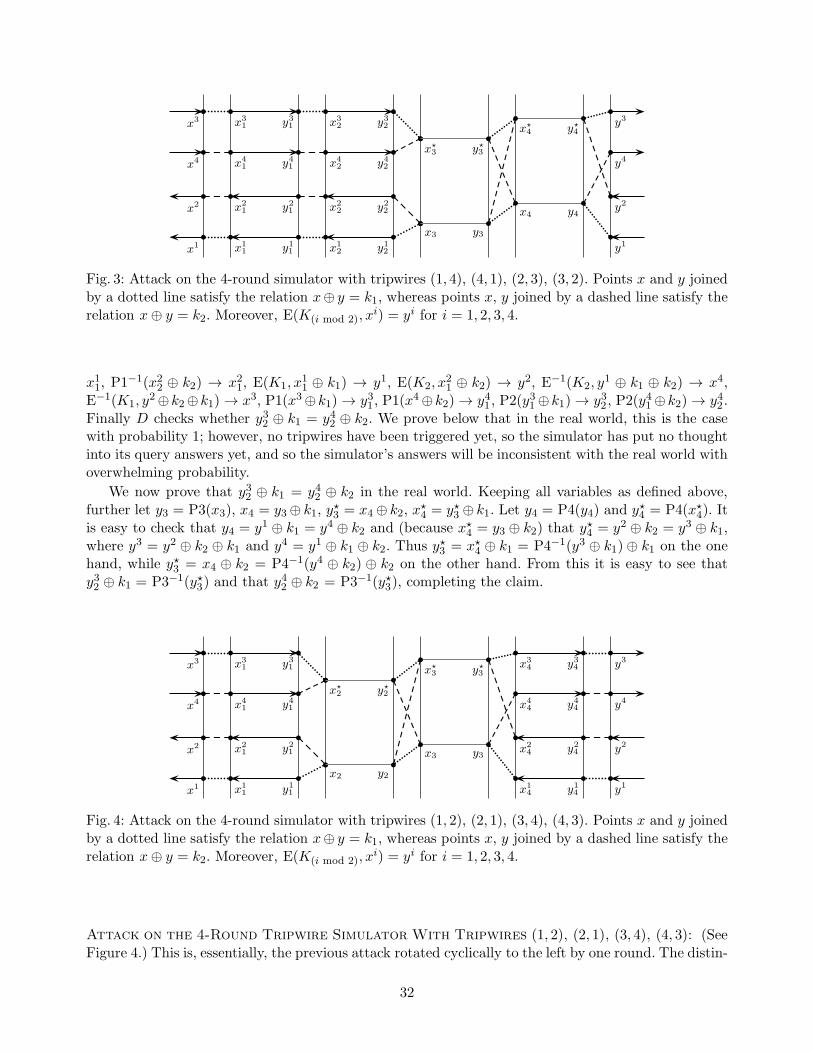
x3

b

b

y12

b

x12

b

y11

b

x11

b

x1

b

b

y22

b

x22

b

y21

b

x21

b

x2

by3

x4

b by4

b

b

y1

y4

x⋆3

b

b

y42

b

x42

b

y41

b

x41

b

x4

b

b

y32

b

x32

b

y31

b

x31

b

x3

b

y⋆3

x⋆4

b b

y⋆4

b

b

y2

y3

Fig. 3: Attack on the 4-round simulator with tripwires (1, 4), (4, 1), (2, 3), (3, 2). Points x and y joinedby a dotted line satisfy the relation x⊕ y = k1, whereas points x, y joined by a dashed line satisfy therelation x⊕ y = k2. Moreover, E(K(i mod 2), x

i) = yi for i = 1, 2, 3, 4.

x11, P1−1(x22 ⊕ k2) → x21, E(K1, x

11 ⊕ k1) → y1, E(K2, x

21 ⊕ k2) → y2, E−1(K2, y

1 ⊕ k1 ⊕ k2) → x4,E−1(K1, y

2⊕k2⊕k1)→ x3, P1(x3⊕k1)→ y31 , P1(x4⊕k2)→ y41 , P2(y

31⊕k1)→ y32 , P2(y

41⊕k2)→ y42 .

Finally D checks whether y32 ⊕ k1 = y42 ⊕ k2. We prove below that in the real world, this is the casewith probability 1; however, no tripwires have been triggered yet, so the simulator has put no thoughtinto its query answers yet, and so the simulator’s answers will be inconsistent with the real world withoverwhelming probability.

We now prove that y32 ⊕ k1 = y42 ⊕ k2 in the real world. Keeping all variables as defined above,further let y3 = P3(x3), x4 = y3⊕ k1, y

⋆3 = x4⊕ k2, x

⋆4 = y⋆3 ⊕ k1. Let y4 = P4(y4) and y⋆4 = P4(x⋆4). It

is easy to check that y4 = y1 ⊕ k1 = y4 ⊕ k2 and (because x⋆4 = y3 ⊕ k2) that y⋆4 = y2 ⊕ k2 = y3 ⊕ k1,

where y3 = y2 ⊕ k2 ⊕ k1 and y4 = y1 ⊕ k1 ⊕ k2. Thus y⋆3 = x⋆4 ⊕ k1 = P4−1(y3 ⊕ k1)⊕ k1 on the one

hand, while y⋆3 = x4 ⊕ k2 = P4−1(y4 ⊕ k2) ⊕ k2 on the other hand. From this it is easy to see thaty32 ⊕ k1 = P3−1(y⋆3) and that y42 ⊕ k2 = P3−1(y⋆3), completing the claim.

x2

b

b

y11

b

x11

b

x1

b

b

y21

b

x21

b

x2

by2

x3

b by3

b

b

x14

x44

b

b

y14

y44

b

b

y1

y4

x⋆2

b

b

y41

b

x41

b

x4

b

b

y31

b

x31

b

x3

b

y⋆2

x⋆3

b b

y⋆3

b

b

x24

x34

b

b

y24

y34

b

b

y2

y3

Fig. 4: Attack on the 4-round simulator with tripwires (1, 2), (2, 1), (3, 4), (4, 3). Points x and y joinedby a dotted line satisfy the relation x⊕ y = k1, whereas points x, y joined by a dashed line satisfy therelation x⊕ y = k2. Moreover, E(K(i mod 2), x

i) = yi for i = 1, 2, 3, 4.

Attack on the 4-Round Tripwire Simulator With Tripwires (1, 2), (2, 1), (3, 4), (4, 3): (SeeFigure 4.) This is, essentially, the previous attack rotated cyclically to the left by one round. The distin-

32

guisher D chooses values x2 and K1, K2, K1 6= K2. ThenD makes the queries f(K1)→ k1, f(K2)→ k2,P1−1(x2⊕k1)→ x11, P1

−1(x2⊕k2)→ x21, E(K1, x11⊕k1)→ y1, E(K2, x

21⊕k2)→ y2, P4−1(y1⊕k1)→ x14,

P4−1(y2 ⊕ k2) → x24, P4(x14 ⊕ k1 ⊕ k2) → y44 , P4(x24 ⊕ k2 ⊕ k1) → y34, E−1(K2, y44 ⊕ k2) → x4,

E−1(K1, y34 ⊕ k1) → x3, P1(x4 ⊕ k2) → y41 , P1(x

3 ⊕ k1) → y31. Finally, the distinguisher checks thaty41⊕k2 = y31⊕k1. No tripwires have been set off, and it is easy to check the attack’s validity by similarobservations as in the last attack (details omitted).

Attack on the 4-Round Tripwire Simulator With Tripwires (1, 2), (2, 3), (3, 2), (4, 3):D chooses values x3 and K1, K2, K1 6= K2. Then D makes the queries f(K1) → k1, f(K2) → k2,P2−1(x3⊕k1)→ x12, P2

−1(x3⊕k2)→ x22, P1−1(x12⊕k1)→ x11, P1

−1(x22⊕k2)→ x21, E(K1, x11⊕k1)→ y1,

E(K2, x21⊕k2)→ y2, P4−1(y1⊕k1)→ x14, P4

−1(y2⊕k2)→ x24. Finally, D checks that x14⊕k1 = x24⊕k2.No tripwires have been set off, and the attack’s validity is easy to check.

Attack on the 4-Round Tripwire Simulator With Tripwires (2, 1), (2, 3), (3, 2), (3, 4):D chooses values x2 and K1, K2, K1 6= K2. Then D makes the queries f(K1) → k1, f(K2) → k2,P1−1(x2⊕k1)→ x11, P1

−1(x2⊕k2)→ x21, E(K1, x11⊕k1)→ y1, E(K2, x

21⊕k2)→ y2, P4−1(y1⊕k1)→ x14,

P4−1(y2⊕k2)→ x24, P3−1(x14⊕k1)→ x13, P3

−1(x24⊕k2)→ x23. Finally, D checks that x14⊕k1 = x24⊕k2.No tripwires have been set off, and the attack’s validity is again easy to check.

Except for the 4-round tripwire simulator with tripwires

(1, 2), (3, 2), (3, 4), (1, 4)

and its symmetric counterpart, other 4-round, 4-tripwire simulators can easily be attacked by variantsof the attacks above (but we omit the case analysis).

B Security Games

See Figures 5–9.

C The Abort Probability of game G2

The main goal of this appendix is the proof of Lemma 1 (stated in Section 4.3) upper bounding theprobability of abortion in game G2. We start with some basic definitions and notations (some of whichare recalled from Section 4). All definitions in this section refer to game G2.

A simulator cycle consists of the execution period starting from when an adversary makes a queryto when the adversary receives an answer. (The answer being, possibly, an abort message.) We alsocount queries to E/E−1 as “simulator cycles”. Hence in G2 the term “simulator” is somewhat liberallyinterpreted as “the code implementing the adversary’s oracle”.

A tuple (i, x, y, dir, num) of the set Queries maintained by the simulator is called an i-query. Weabbreviate i-queries to their first three or four coordinates as convenient. An i-query with dir =→(resp. dir =←) is called random at the right (resp., random at the left). An i-query with dir = ⊥ iscalled adapted. A query (i, x, y, dir, num) is later than a query (i′, x′, y′, dir′, num′) if num > num′;or earlier if num < num′.

We recall that Z is the set of scheduled keys (the image of the table f). Two queries (i, x, y),(i + 1, x′, y′) are adjacent if y ⊕ x′ ∈ Z; we also say two such queries are k-adjacent to mean thaty ⊕ x′ = k ∈ Z.

33

Game G1 G2

Random tapes: p1, . . . , p5, {pE [K] : K ∈ {0, 1}κ}, rf

private procedure ReadTape(Table, x, p)y ← p(x)if (Table(x) 6= ⊥) then abort

if (Table−1(y) 6= ⊥) then abort

Table(x)← yTable−1(y)← xreturn y

public procedure E(K,x)if (ETable[K](x) 6= ⊥) return ETable[K](x)y ← ReadTape(ETable[K], x, pE[K](→, ·))AddEQuery(K,x, y,→) // G2

return y

public procedure E−1(K, y)if (ETable[K]−1(y) 6= ⊥) return ETable[K]−1(y)x← ReadTape(ETable[K]−1, y, pE [K](←, ·))AddEQuery(K,x, y,←) // G2

return x

public procedure f(K)if f(K) 6= ⊥ return f(K)k ← rf (K)KeyQueryChecks(k) // G2

Z ← Z ∪ kf(K)← kf−1(k)← KKeyQueries← KeyQueries ∪ {(K, k,++qnum)}if (qnum > 6q2 + q) then abort

return f(K)

public procedure P1(x)if (P1(x) 6= ⊥) return P1(x)y ← ReadTape(P1, x, p1(→, ·))AddQuery(1, x, y,→)return P1(x)

public procedure P1−1(y)PrivateP1−1(y)Cleanup()return P−1

1 (y)

Game G1 G2 (continued)

private procedure PrivateP1−1(y)if (P−1

1 (y) 6= ⊥) return P−11 (y)

x← ReadTape(P−11 , y, p1(←, ·))

AddQuery(1, x, y,←)FreezeLeftValues(x,⊥)LeftQueue← LeftQueue ∪ (1+, y)return P−1

1 (y)

public procedure P2(x)if (P2(x) 6= ⊥) return P2(x)y ← ReadTape(P2, x, p2(→, ·))AddQuery(2, x, y,→)return P2(x)

public procedure P2−1(y)if (P−1

2 (y) 6= ⊥) return P−12 (y)

x← ReadTape(P−12 , y, p2(←, ·))

AddQuery(2, x, y,←)return P−1

2 (y)

public procedure P3(x)PrivateP3(x)Cleanup()return P3(x)

private procedure PrivateP3(x)if (P3(x) 6= ⊥) return P3(x)y ← ForcedP3(3−, x)if (y 6= ⊥) then

if (y ∈ range(P3)) then abort

P3(x)← yP−13 (y)← x

AddQuery(3, x, y,⊥)RightQueue← RightQueue ∪ (3+, y)

else

y ← ReadTape(P3, x, p3(→, ·))AddQuery(3, x, y,→)

end if

LeftQueue← LeftQueue ∪ (3−, x)return P3(x)

public procedure P3−1(y)PrivateP3−1(y)Cleanup()return P−1

3 (y)

Fig. 5: Games G1 and G2 (first of four sets of procedures). Red lines (commented with ‘// G2’) are ingame G2 only. All other lines belong both to G1 and G2.

A value x3 is called 1-2-joined to a value x1 if there exists a k ∈ Z and 1- and 2-queries (1, x1, y1),(2, x2, y2) such that y1⊕ x2 = y2⊕ x3 = k. (We also say that x1 and x3 are k-1-2-joined, in this case.)Symmetrically, values y3 and y5 are k-4-5-joined if there exists 4- and 5-queries (4, x4, y4), (5, x5, y5)such that y3 ⊕ x4 = y4 ⊕ x5 = k, for some k ∈ Z.

A completed path consists of a 5-tuple of queries (1, x1, y1), . . . , (5, x5, y5) such that there exists avalue k ∈ Z such that (i, xi, yi) is k-adjacent to (i + 1, xi+1, yi+1) for i = {1, 2, 3, 4}, and such thatETable[f−1(k)](x1 + k) = y5 + k. Such a path is also called a k-completed path.

34

Game G1 G2 (continued)

private procedure PrivateP3−1(y)if (P−1

3 (y) 6= ⊥) return P−13 (y)

x← ForcedP3(3+, y)if (x 6= ⊥) then

if (x ∈ domain(P3)) then abort

P3(x)← yP−13 (y)← x

AddQuery(3, x, y,⊥)LeftQueue← LeftQueue ∪ (3−, x)

else

ReadTape(P−13 , y, p3(←, ·))

AddQuery(3, x, y,←)end if

RightQueue← RightQueue ∪ (3+, y)return P−1

3 (y)

public procedure P4(x)if (P4(x) 6= ⊥) return P4(x)y ← ReadTape(P4, x, p4(→, ·))AddQuery(4, x, y,→)return P4(x)

public procedure P4−1(y)if (P−1

4 (y) 6= ⊥) return P−14 (y)

x← ReadTape(P−14 , y, p4(←, ·))

AddQuery(4, x, y,←)return P−1

4 (y)

public procedure P5(x)PrivateP5(x)Cleanup()return P5(x)

private procedure PrivateP5(x)if (P5(x) 6= ⊥) return P5(x)y ← ReadTape(P5, x, p5(→, ·))AddQuery(5, x, y,→)FreezeRightValues(y,⊥)LeftQueue← LeftQueue ∪ (5−, x)return P5(x)

public procedure P5−1(y)if (P−1

5 (y) 6= ⊥) return P−15 (y)

x← ReadTape(P−15 , y, p5(←, ·))

AddQuery(5, x, y,←)return P−1

5 (y)

Game G1 G2 (continued)

private procedure FreezeLeftValues(x1, k⋆)

forall k, k′ ∈ Z do

if (k 6= k′ ∧ x1 ⊕ k ⊕ k′ ∈ domain(P1)) thenabort

end forall // G2

forall k ∈ Z\{k⋆} doif (x1 ⊕ k ∈ LeftFreezer) then abort

forall K ∈ {0, 1}κ do

if (ETable[K](x1 ⊕ k) 6= ⊥) then abort

end forall // G2

LeftFreezer ← LeftFreezer ∪ {x1 ⊕ k}end forall

private procedure FreezeRightValues(y5, k⋆)

... // (symmetric to FreezeLeftValues)

private procedure ForcedP3(i, z)if (i = 3−) then

x3 ← zcandidate← ∅forall k ∈ Z do

if (x3 ⊕ k /∈ range(P2)) continuey1 ← P−1

2 (x3 ⊕ k)⊕ kif (y1 /∈ range(P1)) continuex1 ← P−1

1 (y1)if (x1 ⊕ k ∈ LeftFreezer) continueif (candidate 6= ∅) then abort

candidate← (k, x1 ⊕ k)end forall // (k)if (candidate = ∅) return ⊥(k, x)← candidatey5 ← E(f−1(k), x)⊕ kTallyEQuery(f−1(k), x,→)if (y5 /∈ range(P5)) return ⊥y4 ← P−1

5 (y5)⊕ kreturn P4−1(y4)⊕ k

end if

if (i = 3+) then... // (symmetric to case (i = 3−))

end if

return ⊥

Fig. 6: Games G1 and G2 (second of four sets of procedures).

An execution is the start-to-finish interaction of the distinguisher with G2, including the transcriptof all internal G2 actions. An execution is good or non-aborting if G2 does not abort. We assume, likein Section 4.3, a fixed (deterministic) distinguisher D that completes all chains.

A set of values of the form

{x1 ⊕ k : k ∈ Z, k 6= k∗}

added to LeftFreezer by FreezeLeftValues(x1 , k∗) (where, possibly, k∗ = ⊥) is a left ice tray. We define a

right ice tray similarly. We view ice trays as being “erased” or “removed” at the end of each simulatorcycle (similarly to the erasure of LeftFreezer and RightFreezer at the end of each simulator cycle).

35

Game G1 G2 (continued)

private procedure ExistsPath(i, z, k)if (i = 1+) then

y1 ← zif (y1 /∈ range(P1)) return false

x1 ← P1−1(y1)(ℓ, x)← ProbeForward(2, 5, y1 ⊕ k, k)if (ℓ 6= 5 ∨ x /∈ domain(P5)) return false

if (E(f−1(k), x1 ⊕ k) 6= P5(x)⊕ k) then abort

TallyEQuery(f−1(k), x1 ⊕ k,→)return true

end if

if (i = 3−) thenx3 ← z(ℓ1, y)← ProbeBackward(2, 1, x3 ⊕ k, k)(ℓ2, x)← ProbeForward(3, 5, x3, k)if (ℓ1 6= 1 ∨ y /∈ range(P1)) return false

if (ℓ2 6= 5 ∨ x /∈ domain(P5)) return false

if (E(f−1(k), P−11 (y)⊕k) 6= P5(x)⊕k) then abort

TallyEQuery(f−1(k), P−11 (y)⊕ k,→)

return true

end if

if (i = 3+) then... // (symmetric to case (i = 3−))

end if

if (i = 5−) then... // (symmetric to case (i = 1+))

end if

private procedure ProbeForward(i, j, xi, k)// (i, j ∈ {1, 2, 3, 4, 5}, i < j)while i < j do

if (Pi(xi) = ⊥) breakxi ← Pi(xi)⊕ ki← i+ 1

end

return (i, xi)

private procedure ProbeBackward(i, j, yi, k)// (i, j ∈ {1, 2, 3, 4, 5}, i > j)while i > j do

if (P−1i (yi) = ⊥) break

yi ← P−1i (yi)⊕ k

i← i− 1end

return (i, yi)

Game G1 G2 (continued)

private procedure EmptyQueue()do

while ¬LeftQueue.empty()(i, z)← LeftQueue.pop()if (i = 1+) then ProcessNew1Edge(z)if (i = 3−) then ProcessNew3−Edge(z)

end while

while ¬RightQueue.empty()(i, z)← RightQueue.pop()if (i = 3+) then ProcessNew3+Edge(z)if (i = 5−) then ProcessNew5Edge(z)

end while

while (¬LeftQueue.empty())

private procedure ProcessNew1Edge(y1)forall k ∈ Z

if (ExistsPath(1+, y1, k)) then continue

if (y1 ⊕ k /∈ domain(P2)) then continue

CompletePath1+(y1, k)end forall

private procedure ProcessNew3−Edge(x3)forall k ∈ Z

if (ExistsPath(3−, x3, k)) then continue

if (x3 ⊕ k /∈ range(P2)) then continue

CompletePath3−(x3, k)end forall

private procedure ProcessNew3+Edge(y3)... // (symmetric to ProcessNew3−Edge)

private procedure ProcessNew5Edge(x5)... // (symmetric to ProcessNew1Edge)

private procedure Cleanup()EmptyQueue()LeftFreezer ← ∅RightFreezer ← ∅

private procedure AddQuery(i, x, y, dir)QueryChecks(i, x, y, dir) // G2

Queries← Queries ∪ {(i, x, y, dir,++qnum)}if (qnum > 6q2 + q) then abort

Fig. 7: Games G1 and G2 (third of four sets of procedures).

However, for the time of their existence, ice trays are viewed as “static”, in the sense that removal ofvalues from LeftFreezer or RightFreezer does not affect the ice trays containing those values. (The icetrays are defined as sets, and the sets remain unchanged.) We note that by design, all left ice trayscreated during a simulator cycle are disjoint, and likewise all right ice trays are disjoint, as long as thegame does not abort.

Intuitively, an ice tray holds “certified freshly created random values” that should not have beenqueried before to E (for left ice trays) or E−1 (for right ice trays), under any key. Before queryingthese values to E or E−1 (via EmptyQueue()), such values are carefully removed from LeftFreezer or

36

Game G1 G2 (continued)

private procedure CompletePath1+(y1, k)x1 ← P−1

1 (y1)x3 ← P2(y1 ⊕ k)⊕ kx4 ← PrivateP3(x3)⊕ kx5 ← P4(x4)⊕ kFinishPath1+3−(x1, x5, k)

private procedure CompletePath3−(x3, k)x2 ← P−1

2 (x3 ⊕ k)x1 ← PrivateP1−1(x2 ⊕ k)x4 ← P3(x3)⊕ kx5 ← P4(x4)⊕ kFinishPath1+3−(x1, x5, k)

private procedure FinishPath1+3−(x1, x5, k)if (x1 ⊕ k ∈ LeftFreezer) then

fresh← true

LeftFreezer ← LeftFreezer\{x1 ⊕ k}else

fresh← false

end if

y5 ← k ⊕ E(f−1(k), x1 ⊕ k)TallyEQuery(f−1(k), x1 ⊕ k,→)if (x5 ∈ domain(P5)) then abort

if (y5 ∈ range(P5)) then abort

P5(x5)← y5P−15 (y5)← x5

AddQuery(5, x5, y5,⊥)RightQueue← RightQueue ∪ (5−, x5)if (fresh) then

FreezeRightValues(y5, k)end if

private procedure CompletePath3+(y3, k)... // (symmetric to CompletePath3−)

private procedure CompletePath5−(x5, k)... // (symmetric to CompletePath1+)

private procedure FinishPath5−3+(y5, y1, k)... // (symmetric to FinishPath1+3−)

private procedure TallyEQuery(K, z, dir)if (dir =→) then

if (TallyETable[K](z) = ⊥) then ++EqnumTallyETable[K](z)← t← E(K, z)TallyETable[K]−1(t)← z

end if

if (dir =←) then... // (symmetric to case dir =→)

end if

if (Eqnum > 2q2) then abort

Game G1 G2 (continued)

private procedure AddEQuery(K,x, y, dir) // G2

if (x ∈ LeftFreezer) then abort

if (y ∈ RightFreezer) then abort

if (dir =→) thenforall k, k′ ∈ Z, k 6= k′

if (y ⊕ k ∈ range(P5)) then abort

if (y ⊕ k ⊕ k′ ∈ RightFreezer) then abort

forall K ∈ {0, 1}κ

if ETable[K](y ⊕ k ⊕ k′) 6= ⊥ then abort

end forall

end forall

end if

if (dir =←) then... // (symmetric to case dir =→)

end forall

EQueries← EQueries ∪ {(K,x, y, dir)}

private procedure KeyQueryChecks(k) // G2

if (k ∈ Z) then abort

if ∃ k1, k2, k3, k4 ∈ Z ∪ {k} s.t:(i) k1 ⊕ k2 ⊕ k3 ⊕ k4 = 0(ii) (i 6= j) =⇒ ki 6= kj...then abort

for i = 1 to 4 do

if ∃(xi, yi, xi+1, yi+1) s.t:(i) yi ⊕ xi+1 ∈ (k ⊕ 4Z) ∪ {k}(ii) (i, xi, yi), (i+ 1, xi+1, yi+1) ∈ Queries...then abort

end for

for i = 1 to 5 do

if ∃(xi, yi, x′i, y

′i) s.t:

(i) yi ⊕ y′

i ∈ k ⊕ 5Z ∨ xi ⊕ x′

i ∈ k ⊕ 5Z(ii) (i, xi, yi), (i, x

′

i, y′

i) ∈ Queries(iii) (xi, yi) 6= (x′

i, y′i)

...then abort

end for

private procedure QueryChecks(i, x, y, dir) // G2

if (dir = → ∧ ∃(x′, y′) s.t:(i) (i+ 1, x′, y′) ∈ Queries(ii) y ⊕ x′ ∈ 5Z...) then abort

if (dir = ← ∧ ∃(x′, y′) s.t:(i) (i− 1, x′, y′) ∈ Queries(ii) x⊕ y′ ∈ 5Z...) then abort

if (dir = → ∧ ∃(x′, y′) s.t:(i) (i, x′, y′) ∈ Queries(ii) y ⊕ y′ ∈ 6Z...) then abort

if (dir = ← ∧ ∃(x′, y′) s.t:(i) (i, x′, y′) ∈ Queries(ii) x⊕ x′ ∈ 6Z...) then abort

Fig. 8: Games G1 and G2 (fourth of four sets of procedures). Here, mZ denotes the m-fold direct⊕-sum Z ⊕ · · · ⊕ Z of Z.

37

Game G3

Random tapes: q1, . . . , q5, rf

public procedure E(K,x)k ← rf [K]x1 ← x⊕ kfor i = 1 to i = 4

yi ← qi(→, xi)xi+1 ← yi ⊕ k

end for

return q5(→, x5)⊕ k

public procedure E−1(K, y)k ← rf [K]y5 ← y ⊕ kfor i = 5 to i = 2

xi ← qi(←, yi)yi−1 ← xi ⊕ k

end for

return q5(←, y1)⊕ k

Game G4

Random tapes: q1, . . . , q5, rf

public procedure E(K, x)... // (see G3)

public procedure E−1(K, y)... // (see G3)

public procedure f(K)return rf [K]

public procedure P1(x)return q1(→, x)

public procedure P1−1(y)return q1(←, y)

public procedure P2(x)return q2(→, x)

public procedure P2−1(y)return q2(←, y)

public procedure P3(x)return q3(→, x)

public procedure P3−1(y)return q3(←, y)

public procedure P4(x)return q4(→, x)

public procedure P4−1(y)return q4(←, y)

public procedure P5(x)return q5(→, x)

public procedure P5−1(y)return q5(←, y)

Fig. 9: Left: the functions E and E−1 in game G3 (and renamed randomness for G3); the simulator-related procedures of G3 are the as in G2 (Figures 5-8). Right: game G4.

RightFreezer, such as not to cause abortion. On the other hand we will eventually have to check thatcalls to E and E−1 that occur in ExistsPath (the only procedure in which “unguarded” calls to E, E−1

occur) don’t call E or E−1 on a value in LeftFreezer or RightFreezer respectively. (See Proposition 4far below.)

Invariants. As should be obvious from the functions QueryChecks() and KeyQueryChecks(), amongothers, the simulator of game G2 is a rather “paranoid” simulator that aborts at the first sign oftrouble. This propensity for abortion means good executions are endowed with a certain structure. Welist here five basic invariants (denoted as Inv0 through Inv4) that hold at any point of any execution(good or not) as well as an extra invariant Inv5 that holds at the end of each simulator cycle as longas the simulator has not aborted (Inv5 does not, in general, hold within a simulator cycle); the proofthese invariants hold under the conditions stated is given right below.

Inv0. 2-queries and 4-queries (i.e., queries of the form (j, x, y, dir, num) with j ∈ {2, 4}) have dir ∈{←,→}.

38

Inv1. There does not exist a pair of distinct key queries (K, k, num), (K ′, k′, num′) such that k = k′,nor a 4-tuple of distinct key queries (K1, k1, num1), (K2, k2, num2), (K3, k3, num3), (K4, k4, num4)such that k1 ⊕ k2 ⊕ k3 ⊕ k4 = 0.

Inv2. There does not exist a pair of queries (i, x, y, dir, num), (i+1, x′, y′, dir′, num′) such that either(i) y ⊕ x′ ∈ 5Z, dir =→ and num > num′, or (ii) y ⊕ x′ ∈ 5Z, dir′ =← and num′ > num.

Inv3. There does not exist a pair of queries (i, x, y, dir, num), (i, x′, y′, dir′, num′) such that either: (i)y ⊕ y′ ∈ 6Z, dir = → and num > num′, or (ii) x ⊕ x′ ∈ 6Z, dir = ← and num > num′. [Note thisprecludes the case y ⊕ y′ ∈ 6Z, dir = dir′ =→ as well as the case x⊕ x′ ∈ 6Z, dir = dir′ =←.]

Inv4. If (K,x, y, dir) ∈ EQueries for some K ∈ {0, 1}κ then x /∈ LeftFreezer and y /∈ RightFreezer.

Inv5. The following holds for (i, j) ∈ {(2, 1), (2, 3), (4, 3), (4, 5)}: if (i, xi, yi, dir, num) and (j, xj , yj , dir′,

num′) are two k-adjacent queries such that num′ > num, then these two queries are part of the samek-completed path.

The invariants that we will most frequently appeal to are invariants Inv2, Inv3 and Inv5. In orderto help the reader memorize “which is which” we note that Inv2 concerns the interaction of i-and(i + 1)-queries whereas Inv3 concerns the interaction of i-queries amongst themselves. Inv5 concernsitself with path completion, and states that the tripwires are really “doing their job”.

Lemma 11. Invariants Inv0–Inv4 hold throughout any execution. Invariant Inv5 holds at the end ofeach simulator cycle as long as abort has not occurred.

Proof. We consider each invariant separately:

Inv0: Each time a 2-query or 4-query is created (which occurs only in the procedures P2, P2−1, P4,P4−1), a call to ReadTape occurs and the query is created with direction ← or →. Moreover, querydirections are never modified after creation.

Inv1: This follows from the first two “ifs” in the procedure KeyQueryChecks (the latter procedureis called before each new key scheduling).

Inv2: This follows from the first two “if” blocks in the procedure QueryChecks (this procedurebeing called each time a new query is created) and by the first “for” block of KeyQueryChecks. (Wenote, concerning this for-block, that k /∈ k ⊕ 4Z = ∅ if Z = ∅. The crucial point, here, is that(k⊕ 4Z)∪ {k} ⊇ (5(Z ∪ {k}))\5Z. The latter inclusion is easy to check by considering separately thecases Z = ∅ and Z 6= ∅.)

Inv3: This follows from the second two “if” blocks in QueryChecks and by the second “for” blockin KeyQueryChecks. Here we note that k ⊕ 5Z contains all the elements of 6(Z ∪ {k})\6Z exceptpotentially for the element 0, but 0 has no effect since the fact that Pi is a permutation implies xi 6= x′iand yi 6= y′i for all distinct i-queries (i, xi, yi), (i, x

′i, y

′i).

Inv4: We note that values are added to LeftFreezer, RightFreezer only in procedures FreezeLeft-Values, FreezeRightValues, whereas new tuples are added to EQueries only from within AddEQuery.Thus, Inv4 follows because of the abort condition in the innermost “forall” loop in FreezeLeftValues,FreezeRightValues, and by the two first abort conditions in AddEQuery.

Inv5: We firstly note that when a new key is scheduled (i.e., when a query to f occurs) the newlyscheduled subkey never causes two previously non-adjacent i-, (i + 1)-queries to become adjacent,by the first “for” block in KeyQueryChecks. Thus, by inspection of the procedure EmptyQueue, itis sufficient to show, by symmetry, that (i) whenever a new 1-query (1, x1, y1, dir, num) is createdsuch that there exists an earlier 2-query (2, x2, y2, dir

′, num′) ∈ Queries with y1 ⊕ x2 ∈ Z (Z, here,referring to the set of subkeys already scheduled when the 1-query is created) then (1+, y1) is added

39

to LeftQueue, and (ii) whenever a new 3-query (3, x3, y3, num, dir) is created such that there existsan earlier 2-query (2, x2, y2, dir

′, num′) ∈ Queries with y2 ⊕ x3 ∈ Z (likewise, Z at the momentthe 3-query is created) then (3−, x3) is added to LeftQueue. To prove (i), we note that 1-queriesare only created within the procedures P1, PrivateP1−1 and FinishPath5−3+ (for the latter, see thecorresponding 5-query creation in FinishPath1+3−). For PrivateP1−1 or FinishPath5−3+ the claim isobvious, since the 1-query is automatically added to LeftQueue regardless of anything else. For P1,the new 1-query is not added to LeftQueue, but this 1-query has direction → and causes abortion ifit is k-adjacent to a previous 2-query. The analysis for (ii) is similar: if a new 3-query has direction→ or ⊥ it’s automatically added to LeftQueue, whereas if it has direction ← and it is adjacent to aprevious 2-query it causes abort. ⊓⊔

The Bipartite Graphs B2, B4 and the Graph B

Our next goal is to establish further structural properties of good executions. In particular, we wishto show that certain sets never grow beyond certain bounds in good executions of G2. The relevantmetrics, however, rely on more definitions to be stated.

In particular, we will define an edge-labeled graphB based on the sets Queries andKeyQueries (ormore particularly on Queries and on Z) which conveniently encodes the (most relevant) informationfrom these two sets. Two smaller disjoint graphs B2 and B4 lie at the heart of B, and we describe thesefirst. We emphasize that B as well as B2 and B4 are time-dependent graphs whose contents dependon the state of Queries and Z.

The graphs B2 and B4 are bipartite graphs each of whose two shores is {0, 1}n. B2 depends on Zand on the set of 2-queries, while B4 depends on Z and on the set of 4-queries. For concreteness wedescribe B2. The definition for B4 is entirely analogous.

Edges of B2 are directed and labeled, and constructed as follows: for every 2-query (2, x, y, dir)and every k ∈ Z we construct an edge (x⊕ k, y⊕ k) of label k and of direction dir (i.e., from x⊕ k toy⊕ k if dir =→, the reverse otherwise; by Inv0 this covers all cases). This constitutes all edges of B2.Thus each edge of B2 is associated to a pair comprised of one 2-query and of one element of Z. Wenote that two distinct such pairs cannot give rise to two edges of B2 with the same endpoints by Inv3.(More precisely, if the key value is the same for each pair this is obvious from the fact that P2 is apermutation. If the key values are different are the 2-queries are the same, the endpoints are obviouslydifferent. Finally if the key values are different and the 2-queries are also different, both endpointscannot be the same by Inv0 and Inv3.) Hence, B2 contains no multiple edges. In particular we canassociate a unique 2-query to every pair of nodes joined by an edge in B2, in addition to a unique keyvalue. We also note that edges are added to B2 not only when new queries are created but also whena value is added to Z.

For every 2-query (2, x, y), the set of B2-edges

{(x⊕ k, y ⊕ k) : k ∈ Z}

is called a parallel set of edges, and two edges in this set are called parallel17. Since Z is a set (asopposed to a multiset18) parallel edges have distinct endpoints at either end. We also note that if(x∗, y∗) is an edge of B2 of label k∗, then

{(x∗ ⊕ k∗ ⊕ k, y∗ ⊕ k∗ ⊕ k) : k ∈ Z} (6)

17 As a technical comment, we note that if (x, y), (x′, y′) are parallel edges of B2 then x ⊕ x′ = y ⊕ y′, but the lattercondition is not equivalent to (i.e., does not imply) parallelness. Indeed, two distinct 2-queries (2, x2, y2), (2, x

′2, y

′2)

might have x2 ⊕ x′2 = y2 ⊕ y′

2 without contradicting any of the invariants (even if the existence of such queries isunlikely). Edges are parallel, therefore, if and only if they arise from the same 2-query.

18 Anyway, the same element is never added twice to Z; see Inv1.

40

is the set of parallel edges to (x∗, y∗).

Invariants Inv0–Inv3 imply a number of nice structural properties of B2 and B4, some of whichare collected in the next four lemmas. We emphasize these lemmas state properties that hold at anypoint in any execution.

Lemma 12. Connected components of Bj, j ∈ {2, 4} are directed trees with edges directed away fromthe root. Moreover, the num19 values on the edges of any (necessarily directed) path in Bj are strictlyincreasing.

Proof. By the bracketed remark in Inv3 every vertex of Bj has at most one incoming edge. Next,because queries are totally ordered and edges corresponding to the same query (i.e., parallel edges)don’t share endpoints, two adjacent edges in Bj have different num values and, by Inv3, these num gofrom smaller to larger according to the edge directions. This in particular implies that Bj has no cyclesand, together with the fact that every vertex has indegree at most 1, that connected components ofBj are directed trees. ⊓⊔

Lemma 13. Two parallel edges of Bj , j ∈ {2, 4}, cannot lie on the same directed path. In fact, twoparallel edges cannot lie in the same connected component of Bj.

Proof. The first claim is immediate by Lemma 12. For the second claim, let T be a connected compo-nent of Bj , so that T is a tree with edges directed away from its root. Say that two nodes u, v of T arerelated if u⊕ v ∈ Z ⊕Z, u 6= v, and u and v are either both in an odd level or both in an even level ofT (so that u and v are in the same shore of Bj). Then: (a) T cannot contain a pair of related nodes u,v such that u and v are the heads of edges with different values of num, as this would contradict Inv3,and: (b) T cannot contain a pair of related nodes u, v such that u is the root of T , because then v isat the head of some edge whose num value is greater than the num value of the edge leaving u on thepath towards v, also contradicting Inv3, given that u and v are in the same shore. But if T containstwo parallel edges, then the sources u, v of these edges are related vertices, being in the same shore;in order not to contradict (a) and (b), u and v must be the heads of another pair of parallel edges inT (i.e., edges with equal values of num), which allows to find a new pair of related vertices higher upin the tree; since this regression cannot go on forever (one reaches the root eventually), one concludesthat T cannot contain two parallel edges. ⊓⊔

Lemma 14. Connected components of Bj containing at least one edge never subsequently merge (i.e.,become part of the same connected component of B2 or B4; for j = 2, 4). More precisely, the root of aconnected component of Bj remains forever the root of that component.

Proof. Fix a point in the execution, and let (x, y) be an edge of Bj of label k such that (say) xhas no incoming edges (in particular, the edge (x, y) has direction →) at that point. Assume bycontradiction that, subsequently, a new edge (x, y′) of direction ← appears in Bj. The appearance ofthe new edge (x, y′) can be caused either by the addition of an element to Z or by the creation of anew 2-query. In the latter case the new 2-query has num value greater than the 2-query associatedto (x, y), a contradiction to Inv3. In the former case, let k′ be the newly scheduled subkey and let(j, xj , yj, dirj , numj), (j, x

′j , y

′j , dir

′j , num

′j) be the j-queries respectively associated to the edges (x, y),

(x, y′) of Bj. Then x⊕k = xj , x⊕k′ = x′j, so xj⊕x

′j = k⊕k′ ⊆ k′⊕5(Z\{k′}), which is a contradiction

because it implies the second “for” block of KeyQueryChecks would have aborted before k′ was addedto Z. ⊓⊔

19 Since each edge of Bj is associated to a unique j-query we can unambiguously speak of the “num” value of edges inBj as well as of “earlier” and “later” edges, etc.

41

Here we pause to share some intuition regarding the next lemma, which is maybe a bit more mysteriousthan the previous three. For a change, we give the intuition in terms of the graph B4 (this also fitsbetter with later parts in the proof). We have already noted (Lemma 13) that connected componentsof B2, B4 only contain at most one edge each from every set of parallel edges. On the other hand,note that if (x1, y1), (x2, y2) are two distinct edges in B4 with x1 = x2 and with associated 4-queries(4, x14, y

14), (4, x

24, y

24) and labels k1, k2 then there exists a different component (different component

from the one containing the vertex x1 = x2 = x14⊕ k1 = x24⊕ k2, that is) of B4 that contains a parallelcopy of both of these edges; namely the B4 component containing the two edges

(x14 ⊕ k2, y14 ⊕ k2), (x

14 ⊕ k1, y

24 ⊕ k1)

which indeed lie the same component because x14 ⊕ k2 = x24 ⊕ k1. Hence, every adjacency betweentwo edges in B4 (or B2) is “replicated somewhere else” inside B4 (resp. B2), in the sense that thereexist parallel copies of these two edges that are also adjacent. The content of the following lemma isessentially that a 3-wise adjacency (three edges meeting at a vertex) is, by contrast, never “replicatedsomewhere else” and even, more strongly, that no connected component of B4 contains a parallel copyof all three edges involved in a 3-wise adjacency.

Lemma 15. Let (4, x14, y14), (4, x

24, y

24), (4, x

34, y

34) be three distinct 4-queries such that there exist values

k1, k2, k3 ∈ Z with x14 ⊕ k1 = x24 ⊕ k2 = x34 ⊕ k3. Then no component of B4 contains edges parallelto each of these three 4-queries, except for the component containing the vertex u := x14 ⊕ k1. Thesymmetric statement also applies to the graph B2.

Proof. Let T be a connected component of B4 purportedly containing parallel copies of the 4-queries(4, x14, y

14), (4, x

24, y

24), (4, x

34, y

34), but not containing u. Let ℓ1, ℓ2, ℓ3 ∈ Z be the edge labels on these

parallel copies—i.e., (xi4 ⊕ ℓi, yi4 ⊕ ℓi) is an edge of label ℓi in T for i = 1, 2, 3. Then ℓi 6= ki for all

i since otherwise T would contain u, and ℓi 6= ℓj for i 6= j since xi4 6= xj4. (Indeed, xi4 = xj4 would

also imply yi4 = yj4, as the 4-queries represent a partial permutation.) One can similarly observe thatki 6= kj for i 6= j.

If x14 ⊕ ℓ1 = x24 ⊕ ℓ2 = x34 ⊕ ℓ3 then

ℓi ⊕ ℓj = ki ⊕ kj

for all i, j ∈ {1, 2, 3}, i 6= j. The second half of Inv1 and the fact that ℓi 6= ki, ℓi 6= ℓj then impliesℓi = kj ; but since ℓi = kj for two different j’s, this contradicts the distinctness of k1, k2, k3. We canthus assume without loss of generality that v1 6= v2, where v1 := x14 ⊕ ℓ1, v2 = x24 ⊕ ℓ2.

If neither v1 nor v2 is the root of T then since v1 ⊕ v2 = ℓ1 ⊕ ℓ2 ⊕ k1 ⊕ k2 ∈ 4Z, we obtain acontradiction to Inv3 by considering the two 4-queries associated to the 4-edges whose heads are v1and v2. (These two 4-queries have different values of num by Lemma 13.) On the other hand, a similarcontradiction to Inv3 is obtained if v1 is the root by considering the 4-edge leaving v1 in direction ofv2, and the 4-edge arriving at v2. (These latter two 4-edges are distinct, since v1 and v2 must eitherboth be in even layers, or both be in odd layers of T .) ⊓⊔

We now discuss the graph B, which is a common extension of the graphs B2 and B4 of vertex set({0, 1}n)6. Basically, B is obtained by “gluing” together B2 and B4 with queries of the form (3, x, y),and by gluing extra pendant edges to the left shore of B2 (one for every query of the form (1, x, y))and to the right shore of B4 (one for every query of the form (5, x, y))20. The additional glued edgesare unlabeled, by contrast to the edges of B2 and B4.

20 At this juncture we warn about a potential source of confusion: we often refer to a generic edge of B2 as “(x, y)” whenthe left shore of B2 actually corresponds to “y1 values” (outputs of P1) and the right shore corresponds to “x3 values”

42

More precisely, B has six “shores” equal to {0, 1}n; a copy of B2 is placed between shores 2 and3, whereas a copy of B4 is placed between shores 4 and 5. For i = 1, 3, 5, a query (i, x, y) becomes a(possibly directed) unlabeled edge from node x in shore i to node y in shore i+1. Edge directions areascribed the natural way; for example, query (1, x, y, dir, num) becomes an edge directed from shore1 to shore 2 if dir =→, and so on; queries with dir = ⊥ become undirected edges. Edges also inheritthe “timeline” of their associated queries, so that we can speak of “earlier” and “later” edges of B.(As we know, not all edges of B are comparable this way, since some edges of B2 and B4 correspondto the same query.)

We note that every query of the form (1, x, y), (3, x, y) or (5, x, y) corresponds to exactly one edgein B, by contrast to queries of the form (2, x, y) and (4, x, y) that correspond to |Z| edges in B. Wealso note that a k-completed path of queries corresponds to a path of 5 edges in B, starting in shore1 and ending on shore 6, such that both labeled edges are labeled by k, and such that the endpointsof the path are compatible with Ef−1(k). (The labeled edges being the residents of B2 and B4; forconvenience, we will identify B2 and B4 with their copies in B.) Moreover, every edge of B2 and B4

is in at most one k-completed path, because of its label.

For shorthand, an i-edge of the graph B is an edge between shores i and i + 1; thus i-edgescorrespond to i-queries. However, this correspondence is only 1-to-1 for i = 1, 3, 5. We will occasionally,for the sake of convenience, confuse the notion of “i-edge” and “i-query” for i = 1, 3, 5, but we willcarefully keep the two notions separate for i = 2, 4. We note that the set of all i-edges forms a partialmatching between shores i and i + 1 for i = 1, 3, 5 (because these edges encode the partially definedpermutations P1, P3 and P5). In particular, every node in shore 2 is adjacent to at most one 1-edge,etc.

The notion of “1-2-join” translates as follows into the graph B: a value x3 in shore 3 is “k-1-2-joined” to a value x1 in shore 1 if and only if there is a path of length two (edge directions ignored)from x1 to x3 where the 2-edge of the path has label k. Symmetrically for “4-5-join”.

Invariant Inv5 above translates as follows into the graph language: for (i, j) ∈ {(2, 1), (2, 3), (4, 3),(4, 5)}: if an i-edge and j-edge are adjacent, but not in a completed path, the j-edge must be earlierthan the i-edge. Moreover, the i-edge must therefore be directed “away” from the j-edge, in order notto contradict Inv3.

Invariants Inv2 and Inv3 above imply, in particular, the following: if an edge e of B is adjacentto a {←,→}-directed edge e′ of B, such that e and e′ are adjacent at the “arrow end” of e′ (i.e., the“head” of e′), then e must be a later edge than e′.

We note that each tuple added to LeftQueue and RightQueue is associated to a unique 1-edge,3-edge or 5-edge in the obvious way. We will therefore sometimes speak of a 1-edge (or 3-edge, etc)being “added to LeftQueue” or “popped from LeftQueue” with the obvious intent.

To re-emphasize, and for future reference, the left and right shores of B2 are shores 2 and 3 of Bwhile the left and right shores of B4 are shores 4 and 5 of B.

Pebbling. A node in shore 2, 3, 4 or 5 of B that is adjacent to a 1-edge, 3-edge or 5-edge is said tobe pebbled. In this case we also say the node is pebbled by the relevant 1-, 3- or 5-edge. Note the edgepebbling a node necessarily unique. One can also note that nodes in shore 2 can only be pebbled by1-edges, that nodes in shores 3 and 4 can only be pebbled 3-edges, and that nodes in shore 5 can onlybe pebbled by 5-edges.

The following property of pebbling plays a crucial role in our proof:

(inputs of P3). (Thus x refers to a y1-value while y refers to an x3-value.) Similarly the left and right shores of B4

correspond to y3- and x5-values respectively, even though an edge of B4 is generically called “(x, y)”. Along the samelines, inputs and outputs to the cipher E are generically labeled x, y when more logical names might be y0 and x6,instead.

43

Lemma 16. At any moment of execution such that Inv5 holds the connected components of B2 andB4 are “pebbled upwards”: if a node in a connected component of Bj is pebbled, then so is the parent ofthat node (recall the connected component is a directed tree by Lemma 12). In particular, if any nodeof a component is pebbled, then so is the root.

Proof. Let x3 be, say, a pebbled node in shore 3 such that there exists a 2-query of the form (2, y1 ⊕k, x3⊕ k,→, num) for some k, num; in other words, the vertex x3 has parent y1 in B2 (via an edge oflabel k). Because of the direction y1 → x3 of the edge (y1, x3) in B2, the 3-edge adjacent to x3 mustbe a later edge than the edge (y1, x3) ∈ B2 in order not to contradict Inv3; which means by Inv5 thatthere exists a completed path containing that edge and the edge (y1, x3) ∈ B2. But the presence of apath means y1 is pebbled by a 1-edge. Other cases are symmetric. ⊓⊔

Live trees.We writeBj(v) for the connected component containing a node v in Bj . We will be especiallyinterested in the size of the largest connected component of Bj formed by non-pebbled nodes. We clarifythis with a definition.

Fix a moment in the execution when Inv5 holds. Let v be a non-pebbled vertex of Bj. Then Bj(v)is a directed tree with edges directed away from the root. Let u be the highest non-pebbled node inBj(v) above v (possibly u = v). Then no nodes beneath u are pebbled (or else u would already bepebbled). If u is not the root, let u be the parent of u in Bj(v). Let Bj(v)

− be obtained from Bj(v)by removing all nodes whose (undirected) path to v passes through u, if u exists, but not removing uitself. We define the live tree anchored at v Li(v) to be the tree obtained by “dangling” Bj(v)

− by v,i.e., making v the new root of the tree. One can note that Li(v) is no longer a directed tree in the senseof having all edges directed towards/away from the root (in fact, edge directions will no longer beimportant to us in Li(v)), and that at most one node of Li(v) is pebbled, namely u, which, if present,is a leaf in Li(v).

We note that Li(v) = {v} if v is not adjacent to any edges. For convenience, we also defineLi(v) = {v} if v is a pebbled node.

The above definition of Li(v) presupposes that Inv5 holds. It will be convenient, however, if Li(v) isdefined for all nodes v at all moments of execution. For this we use the following generalized definition:Li(v) is the tree obtained by “dangling” the connected component of Bj containing v by v, such that vis the root, and then pruning all portions of the “dangled” tree that lie beneath a pebbled node (thusa non-leaf node of the tree is never pebbled, and Li(v) reduces to v if v is pebbled). It is easy to seethis definition is indeed a generalization of (i.e., compatible with) the original definition of Li(v).

The size of Li(v) is the number of non-pebbled nodes in Li(v). We define

γ(Bj) = maxv

size(Li(v))

where the max is taken over all vertices of Bj . We also define

γ(B) = max{γ(B2), γ(B4)}.

As we will see, γ(B) is closely related to maximum running time of a simulator cycle.

Fans and brooms. We make a last few special-purpose definitions that will be convenient for the proofsin the next subsection.

A (maximal) connected component of B4 consisting of a single vertex in shore 4 connected to tdifferent vertices in shore 5, with all t edges having direction →, is called a rightward B4-fan of degreet. (We note t ≤ |Z|, for obvious reasons.) The vertex in shore 4 is called the apex of the fan. Theunion of all edges that are parallel to edges in a rightward B4-fan F is called the parallel completion

44

of F . We note that because each edge in a B4-fan has a different label k, different edges of a B4-fan donot undergo the exact same “parallel duplication” process, cf. (6). Thus the parallel completion of aB4-fan of degree t is not simply the disjoint union of |Z| different B4-fans of same degree t. Indeed, it iseasy to see from Inv321, from Lemma 15 and from the remarks preceding that lemma that the parallelcompletion of a B4-fan of degree t consists of

(

t2

)

(disjoint) B4-fans of degree 2, of (|Z| − 1)t − 2(

t2

)

(disjoint) B4-fans of degree 1, and of the original B4-fan of degree t.The parallel completion of is called self-contained if no edges of B4 outside the parallel completion

are adjacent to any edges inside the self-completion. By the above remarks we have

size(Li(v)) ≤ 3

for every vertex v in the parallel completion of a self-contained fan such that v is not in the samecomponent as the fan’s apex.

A natural process for constructing a rightward B4-fan, that will occur many times below, is asfollows: (i) a 3-query (3, x3, y3,→) of direction → is created; (ii) a number of 4-edges of direction →adjacent at the left to y3 are subsequently created; more precisely, the i-th such edge comes about asthe result of a new 4-query (4, y3⊕ki, . . . ,→) being created, for some sequence of values k1, . . . , kt ∈ Z.If the process just described doesn’t cause abort to occur, and if no other queries are created than theones just described, it is easy to see that the resulting B4-fan of degree t that is created is self-containedregardless of the previous state of B4. (This uses, in particular, Inv2; for when we select a randomvertex y3 in shore 4 as the head of the 3-edge and as the fan’s apex, we need y3 to be selected suchthat there do not exist values k, k′, k′′ ∈ Z and x4 ∈ domain(P4) such that

y3 ⊕ k ⊕ k′ = x4 ⊕ k′′.

Indeed, note that the set{y3 ⊕ k ⊕ k′ : k, k′ ∈ Z}

is a superset of the shore 4 vertices in the parallel completion of any fan of apex y3, whereas the set

{x4 ⊕ k′′ : x4 ∈ domain(P4), k′′ ∈ Z}

is the set of all shore 4 vertices already adjacent to an edge in B4. As for adjacencies in shore 5, thesecannot be created because of Inv3 and the fact that the newly created 4-queries all have direction →.)

It is also easy to see (the arguments are the same) that if the above two-step process is interleavedfor several fans at once the resulting set of fans created each have a self-contained parallel completion,presuming abort doesn’t occur. Furthermore, if other non-4-queries are created at the same time thisobviously doesn’t change anything either (as the final condition concerns B4). In fact, new 4-queriescan also be created during the fan creation process without affecting the self-containment of fans aslong as each such newly created 4-query is “anchored in B4”; i.e., as long as x4⊕Z is a shore 4 vertexadjacent to a previous edge of B4 for each new 4-query of the form (4, x4, y4,→) and as long as y4⊕Zis a shore 5 vertex adjacent to a previous edge of B4 for each new 4-query of the form (4, x4, y4,←).(The details all involve Inv2 and Inv3, and the arguments are entirely similar to above.)

A 3-edge of direction → attached to a rightward B4-fan, where each edge of the B4-fan is ad-ditionally attached to a 5-edge of direction ⊥, is called a B4-broom; the parallel completion of thebroom is obtained by adding the parallel completion of the B4-fan to the broom. We say the broom isself-contained if the broom’s fan has a self-contained parallel completion. Importantly, one can notethat

size(Li(v)) ≤ 3

21 Inv3 precludes edges in the parallel completion from having adjacencies in shore 5.

45

for every vertex v of B4 adjacent to an edge in the parallel completion of a self-contained broom, sincethe vertices inside the fan are pebbled (and hence have size(Li(v)) = 0).

Symmetric definitions (leftward fan, broom, etc) hold for B2. For example, the apex of a leftwardB2-fan is a shore 3 vertex.

Inside the Simulator Cycle

In the previous subsection we mainly introduced the graphs B2, B4 and B, the metrics γ(B2), γ(B4)and γ(B) and notions of fans and brooms. In this section our main concern is to bound the maximumper-simulator-cycle growth of γ(B) as well as of the sets Queries, KeyQueries and EQueries. Recallthat a “simulator cycle” is the portion of execution allotted to answering a single adversarial query.The upper bounds we obtain depend on the type of adversarial query, and a schematic summary ofthe results is given in Table 1. (The two γ(B)’s appearing in the last row of this table refer, moreprecisely, to the value of γ(B) at the start of the simulator cycle.)

Unsurprisingly, simulator cycles that answer an adversarial query to f, P1, P2±1, P4±1 or P5−1

are quite easy to analyze whereas all other simulator cycles (namely those answering a query to P1−1,P3±1 and P5) are quite involved to analyze. Hence the upper bounds are proved in two separatelemmas, for the “easy” and “hard” cases. The following lemma covers the “easy” cases of Table 1:

Table 1: Bounds on the growth of key quantities per adversarial query.

adds at most . . . to: γ(B) |KeyQueries| |Queries| |EQueries| Lemma

query to E or E−1 0 0 0 1 17

query to f 0 1 0 0 17

query to P1 or P5−1 0 0 1 0 17

query to P2, P2−1, P4 or P4−1 2 0 1 0 17

query to P1−1, P3, P3−1 or P5 2 0 6γ(B) 2γ(B) 18

Lemma 17. An adversarial query to E, E−1, f, P1, P2, P2−1, P4, P4−1 or P5−1 influences the valuesγ(B), |KeyQueries|, |Queries| and |EQueries| as follows:

– γ(B) is increased by at most 2 in queries to P2, P2−1, P4 or P4−1, and by 0 in other queries.– |KeyQueries| is increased by at most 1 in queries to f, and by 0 in other queries.– |Queries| is increased by at most 1 in queries to P1, P2, P2−1, P4, P4−1 or P5−1, and by 0 in

other queries.– |EQueries| is increased by at most 1 in queries to E or E−1, and by 0 in other queries.

Proof. We examine each quantity separately:

– γ(B). Note that γ(B2) is defined by P2 only. An adversarial query to E, E−1, P1, P4, P4−1 orP5−1 clearly does not add new elements to P2 (particularly as procedure EmptyQueue() is neverevaluated). A query to P2 or P2−1 increases γ(B2) by at most one by Lemmas 13 and 14. (Thisalso holds if B2 is empty to start with, since γ(B2) = 1 if B2 is empty.) Each query to f adds asmany edges to B2 as there are 2-queries (unless abort occurs). However these new edges all go intotheir own isolated component because of the second “for” loop in KeyQueryChecks and, hence,

46

γ(B2) can only augment by 1 as a result. As similar bounds hold for γ(B4) the claims on γ(B)follow.

– KeyQueries. This is obvious: an adversarial query to f results in at most one new element addedto KeyQueries whereas queries to other public functions don’t increase the number of scheduledsubkeys as the simulator never calls f. (Indeed, outside f the simulator only uses the set Z and thetable f−1.)

– Queries. In a query to P1, P2, P2−1, P4, P4−1 or P5−1, procedure EmptyQueue() is never evalu-ated, and at most one element is added to Queries. An adversarial query to E, E−1 or f does notresult in new elements.

– EQueries. An adversarial query to E or E−1 results in at most one new element added to EQueries.Queries to f, P1, P2, P2−1, P4, P4−1 or P5−1 do not result in calls to E or E−1. ⊓⊔

The following lemma proves the “hard part” of Table 1. In many ways, this lemma’s proof constitutesthe heart of our whole analysis (and is therefore worth spending some time on despite its depressinglength).

Lemma 18. An adversarial query to P1−1, P3, P3−1 or P5 affects γ(B), |KeyQueries|, |Queries|and |EQueries| as follows: γ(B) is increased by at most 2, |Queries| increases by at most 6γ(B)(referring to the value of γ(B) at the start of the simulator cycle), and |EQueries| increases by atmost 2γ(B) (ditto). Any of these queries leaves KeyQueries invariant.

Proof. The fact that KeyQueries is left unchanged is obvious, since the simulator doesn’t query finternally. For the remaining statements we only consider queries to P1−1 and P3, which is sufficientby symmetry. We start by considering a query to P1−1.

Assume the adversary makes a query P1−1(y∗1). If y∗1 is adjacent to a 1-edge then the simulator

returns immediately, so we can assume that y∗1 is not adjacent to a 1-edge when the query P1−1(y∗1)is made, i.e. that y∗1 is unpebbled at that moment. We let Ty∗1

be the live tree Li(y∗1) as it stands atthe start of the simulator cycle. (The purpose of “renaming” Li(y∗1) as Ty∗1

is to avoid ambiguity, sinceLi(y∗1), technically, changes during the simulator cycle; by our definition, Ty∗1

is a specific “snapshot”of Li(y∗1).) We note that Ty∗1

has at least one non-pebbled node, namely y∗1 itself, and that y∗1 is theroot of Ty∗1

. If y∗1 is the unique vertex of Ty∗1then “nothing happens” when the query P1−1(y∗1) is

made (more precisely, a 1-edge of direction ← is lazy-sampled, added to LeftQueue, then LeftQueue isemptied with nothing happening, and the simulator returns). We will therefore assume that Ty∗1

hasat least two nodes in what follows.

Recall that Ty∗1has either one or zero pebbled leaves, since Inv5 holds at the beginning of the

simulator cycle (see the original definition of a live tree). We divide the analysis into three casesaccording to whether Ty∗1

has a pebbled leaf or not, and if so in which shore.

Case 1: Ty∗1has no pebbled leaf. G2 starts by adding an edge (1, x∗1, y

∗1 ,←, num) where x∗1 is chosen

randomly. At this point the values {x∗1⊕k : k ∈ Z} are added to LeftFreezer (which in fact consists onlyof those values, since LeftFreezer starts out empty). (If abort does not occur22 then we are guaranteed,in particular, that ETable[K](x∗1 ⊕ k) = ⊥ for every K ∈ {0, 1}κ and every k ∈ Z, by the checksmade in FreezeLeftValues.) The pair (1+, y∗1) is finally added to LeftQueue. Before this LeftQueue, likeRightQueue, is empty. Then EmptyQueue is called.

[Some handy vocabulary: In a nutshell, now, the new 1-edge (1, x1∗, y∗1 ,←) will be popped from

LeftQueue, and the simulator will complete a path for every child of y∗1 in Ty∗1; these children of y∗1

22 While the lemma still holds for simulator cycles during which abort occurs we will tacitly carry out the analysisassuming abort doesn’t occur. Checking that nothing extraordinary happens if abort occurs (which isn’t importantanyway for the rest of the proof) is left to the reader.

47

will therefore become pebbled by 3-edges, and these 3-edges are added to LeftQueue; when each 3-edge is popped from LeftQueue, third-level nodes of the tree become pebbled by 1-edges that are alsoadded to LeftQueue, and so on. As a convention, we say that a node of the tree is processed whenthe 1- or 3-edge containing it is popped from LeftQueue and the relevant call to ProcessNew1Edgeor ProcessNew3−Edge is made (i.e., the call containing the node’s name); during that same call, wesay that the node’s children are pre-processed. For example, when the first element (1+, y∗1) is poppedfrom LeftQueue and ProcessNew1Edge(y∗1) is called, we say that y∗1 is processed and that the childrenof y∗1 in Ty∗1

are pre-processed by the call.]

Let x13, . . . , xℓ3 be the children of y∗1 in Ty∗1

(these are “second-level” nodes of the tree) and let kj be

the label on the 2-edge (y∗1, xj3). We assume the children x13, . . . , x

ℓ3 are ordered such that k1 < . . . < kℓ,

and that a loop of the type “forall k ∈ Z” iterates from the smallest value of k ∈ Z to the largest.(We will make similar ordering assumptions without mention in the future.)

As per our convention above, y∗1 is “processed” when the pair (1+, y∗1) is popped off LeftQueue andProcessNew1Edge(y∗1) is called. Within that call, the first child x13 of y∗1 is “pre-processed” when the“forall” loop in ProcessNew1Edge iterates with k = k1. At this point, CompletePath1+(y∗1, k

1) is called,and PrivateP3(x13) is called from within the latter function. Because Ty∗1

has no pebbled leaves to startwith, P3(x

13) = ⊥ at this point. Moreover, the only value x1 that x13 is k-1-2-joined to for some k ∈ Z

is x1 = x∗1, with k = k1, and we have x∗1 ⊕ k1 ∈ LeftFreezer. Thus ForcedP3(x13) will return ⊥ when itis called by PrivateP3(x13), and PrivateP3(x13) creates a new 3-edge (3, x13, y

13,→) by calling ReadTape.

This new 3-edge is added to LeftQueue. Then CompletePath1+ creates a new 4-query (4, y13⊕k1, y14,→)

(indeed, this query will be new because otherwise its adjacency to the newer query (3, x13, y13) would

contradict Inv2), removes x∗1⊕k1 from LeftFreezer, and finally creates a new 5-query (5, y14⊕k1, y15 ,⊥)where y15 = Ef−1(k1)(x

∗1 ⊕ k1) ⊕ k1. (We note in passing that since Ef−1(k1)(x

∗1) is randomly sampled

at this point, y15 /∈ range(P5) or else E would abort from within AddEQuery. Moreover y14 ⊕ k1 cannotbe in domain(P5), either, without contradicting Inv2, the 4-query (4, y13 ⊕ k1, y14,→) being new.)

The new 3-query (3, x13, . . .) and the new 5-query (5, x15, . . .) each correspond to a new 3-edge and5-edge of directions → and ⊥ respectively that are added to B, while the new 4-query (4, x14, . . .)becomes a collection of |Z| different parallel 4-edges added to B4 ⊆ B, where only one of these 4-edges(i.e., the one with label k1) is adjacent to the newly created 3-edge and 5-edge; the other newly created|Z| − 1 4-edges are, by Inv2 and Inv3, not adjacent to any previous edges of B. Thus, the parallelcompletion of a self-contained “degree 1 B4-broom” (i.e., broom whose fan has degree 1) is added toB.

The pre-processing of subsequent second-level nodes of Ty∗1(via the same call ProcessNew1Edge) is

not affected by the degree 1 B4-broom added by the pre-processing of x13, or by the removal of x∗1⊕ k1

from LeftFreezer, since each such second-level node is connected to y∗1 by a 2-edge of different label.Thus, since Ty∗1

has ℓ second-level nodes, ℓ parallel completions of degree 1 brooms are sequentiallyadded to B as the game pre-processes the second-level nodes of Ty∗1

and all these parallel completionsare self-contained.

Let (xj3, yj3) be the 3-edge (broom “handle”) containing xj3. We also point out (since this will shortly

play a role), that the sets{yj3 ⊕ k : k ∈ Z} and {yi3 ⊕ k : k ∈ Z} (7)

are disjoint from one another for i 6= j, by Inv3, and also that

{yj3 ⊕ k : k ∈ Z, k 6= kj} ∩ domain(P4) = ∅ (8)

after the pre-processing of second-level nodes, by Inv2.We also note that while the newly created 5-edges are placed on RightQueue, they will later be

“innocuously popped” from the queue, being adjacent to a single 4-edge with whom they are part

48

of a completed path. (The fact that these newly created 5-edges indeed remain adjacent to a single4-edge—i.e., that new adjacent 4-edges aren’t added—will follow by Inv2 and by the analysis below.)

To describe the processing of second-level nodes of Ty∗1, let x3 be the first second-level node with

at least one child and let y11, . . . , yt1 be the t third-level children of x3 in Ty∗1

(these are nodes in shore

2 of B). Let kj be the label on the 2-edge from x3 to yj1 (note that above, we used kj , not kj—thuswe are not (yet) overwriting our definitions), and let k∗ be the label on the 2-edge from x3 to y∗1. Wenote k∗ 6= k1, . . . , kt since all these are labels of distinct 2-edges adjacent at the same node x3 of B2.(Confusingly, we also note that k∗ = kj for some j, because k1, . . . , kℓ are the labels of the 2-edgesleaving y∗1.) Also, let (x3, y3) be the 3-edge containing x3.

When (3−, x3) is popped from LeftQueue, ProcessNew3−Edge(x3) is called and iterates its “forall”loop. When the “forall” loop iterates with k = kj an adjacency with a 2-edge is detected and, since yj1 isunpebbled (in particular, not in any completed path), CompletePath3−(x3) is called. CompletePath3−

starts by creating a new query (1, xj1, yj1,←), and the values {xj1 ⊕ k : k ∈ Z} become a new ice tray.

Then CompletePath3− makes the call P4(P3(x3) ⊕ kj) (equivalent to P4(y3 ⊕ kj)), which resultsin the creation of a new 4-query (4, x4,j , y4,j ,→) with x4,j = y3 ⊕ kj . The query (4, x4,j , y4,j,→)is new, indeed, because y3 ⊕ kj /∈ domain(P4), as per the remarks above (cf. (7) and (8)), given

that kj 6= k∗. Next xj1 ⊕ kj is removed from LeftFreezer (indeed, no modification of LeftFreezer has

occurred since the (recent) creation of the edge (1, xj1, yj1,←)) and the value y5,j = Ef−1(kj)(x

j1 ⊕ kj)

is computed. Again, since xj1 ⊕ kj is a “fresh” call to Ef−1(kj) that involves calling AddEQuery,y5,j /∈ range(P5) or else AddEQuery would abort, and since the 4-query (4, x4,j , y4,j ,→) is new we alsohave y4,j ⊕ kj /∈ domain(P5) by Inv2. Thus, with high probability23, the game adds a new 5-query(5, y4,j ⊕ kj , y5,j,⊥) without aborting. We note that (y3, y4,j ⊕ kj) becomes a new 4-edge in B4, alongwith its attendant parallel edges.

Carrying out the above process for j = 1, . . . , t has the effect of creating a B4-broom of degree t+1,where the, “handle” of the broom is the query (3, x3, y3,→) and where edge labels on the broom’s fanare k∗, k1, . . . , kt. The broom is self-contained, as it follows the canonical “two-step creation process”described in our introduction to brooms. We can also note that the broom’s degree is exactly equalto the degree of the second-level node x3 in Ty∗1

(edge to parent included). Hence, the net effect ofprocessing the new 3-edge (3, x3, y3,→) in ProcessNew3−Edge is the creation of a self-contained B4-broom whose degree is the same as that of x3 in B2. We note again that the new 5-edges of direction⊥ created (the “broom hairs”) are adjacent to only one 4-edge, with whom they lie on a completedpath.

While the above assumed for simplicity that x3 was the first second-level child of y∗1 with third-levelchildren, nothing substantive changes when processing subsequent second-level nodes: each second-levelnode gives rise to a self-contained broom of degree equal to its own degree in Ty∗1

.

The processing of level 3 nodes is similar to the processing of the level 1 node y∗1. More precisely,let yj1 be a level 3 node (as in the third-to-last paragraph), with associated 1-edge (1, xj1, y

j1,←) added

(as just described) during the processing of x3 and during the pre-processing of yj1. Then level 4 nodes

beneath yj1 are pre-processed the same way with respect to the (newly created) 1-edge (xj1, yj1) as level

2 nodes were pre-processed with respect to the (then newly created) 1-edge (x∗1, y∗1). In particular, the

presence of the 2-edge (yj1, x3) of label kj1 has no effect because this edge is in a completed kj1-path, and

is therefore ignored by ProcessNew1Edge(yj1). Subsequently, level 4 nodes are processed similarly tolevel 2 nodes, and so on. The interleaved, “breadth-first search” aspect of the Ty∗1

traversal obviouslymakes no difference either.

23 But we emphasize that the probability of abortion is not this lemma’s topic. Phrases such as “with high probability”are only included for readability (to remind that abort might have occurred, and in which case we basically don’tcare) and have no mathematical intent.

49

In summary, as a result of the game answering the query P−11 (y∗1), no new edges are added to B2,

while some new edges are added to B4. The edges added to B4 are in (the parallel completions of)self-contained B4-brooms; each B4-broom is associated to an even-level node in Ty∗1

, and the degree ofthe broom equals, exactly, the degree of that node in Ty∗1

. Because

size(Li(v)) ≤ 3

for every shore 4 and shore 5 vertex v in the completion of a self-contained broom, we therefore seeγ(Bj), j = 2, 4, increase by at most 2 (i.e., from 1 to 3) as a result of the game answering the queryP−11 (y∗1).

Each odd-level node in Ty∗1causes the game to create one new 1-query (including y∗1 itself), whereas

each even-level node of degree t (edge to parent included) causes the game to create one new 3-query, tnew 4-queries, and t new 5-queries (all part of the same broom). Thus, some simple accounting showsthat the total number of queries created by the game is

|V (Ty∗1)|+ 2|E(Ty∗1

)|

where V (Ty∗1) is the vertex set of Ty∗1

and E(Ty∗1) is the edge set of Ty∗1

. Since a tree with m verticeshas (at most) m− 1 edges, the number of queries created by the game is therefore at most

|V (Ty∗1)|+ 2(|V (Ty∗1

)| − 1) ≤ 3 · size(Ty∗1) = 3 · sizeLi(y∗1) ≤ 3γ(B)

since size(Ty∗1) = |V (Ty∗1

)|, where the last two quantities refer to the start of the simulator cycle.Finally, the number of calls to E is one for each edge of Ty∗1

, so the simulator makes at most size(Ty∗1)

calls to E. This concludes our analysis of case 1.

Case 2. Ty∗1has a pebbled leaf at an even-level node (i.e., a node in shore 3). Let x◦3 = u be the

pebbled leaf of Ty∗1and let (x◦3, y

◦3) be the 3-edge adjacent to that leaf. Let y◦1 be the odd-level parent

of x◦3 in Ty◦3(possibly y◦1 = y∗1), and let k◦ be the label of the edge (y◦1 , x

◦3) in B2. We consider two

different subcases, according to whether y◦3 is or is not adjacent to a 4-edge of label k◦ at the start ofthe simulator cycle.

Subcase 2.1. y◦3 is adjacent to a 4-edge of label k◦. Let (y◦3, x◦5) be the 4-edge of label k◦ and let

Tx◦5= Li(x◦5) as this tree stands at the start of the simulator cycle. We first argue that x◦5 cannot be

in a 5-edge (x◦5, y◦5) when the adversary makes the query P−1

1 (y∗1). Indeed, if this were the case, thenbecause the 4-edge (y◦3 , x

◦5) has a direction (← or →) either the 5-edge (x◦5, y

◦5) or the 3-edge (x◦3, y

◦3)

would have to be later than the 4-edge (y◦3, x◦5), placing all three edges (x◦3, y

◦3), (y

◦3, x

◦5) and (x◦5, y

◦5)

on a common k◦-completed path, together also with the 2-edge (y◦1, x◦3) of label k

◦; but then y◦1 wouldhave to be adjacent to a 1-edge, a contradiction to the fact that x◦3 is the only vertex of Ty∗1

adjacentto a 3-edge or 1-edge. Thus, x◦5 is not adjacent to a 5-edge, and Tx◦

56= {x◦5}; in fact we know the tree

Tx◦5has a pebbled leaf, this being y◦3, as y

◦3 is adjacent to a 3-edge at the start of the simulator cycle,

and as (y◦3 , x◦5) is a 4-edge.

When G2 processes the tree Ty∗1, at some point an edge (1, x◦1, y

◦1 ,←) is created and put onto the

queue (maybe right away, if y◦1 = y∗1). When the edge (1, x◦1, y◦1,←) is popped from the queue and

y◦1 is processed, the game eventually executes the body of the “forall” loop in ProcessNew1Edge(y◦1)with k = k◦. ProcessNew1Edge() will call PrivateP3(x◦3) to learn y◦3 (and to no other effect, since the3-query (3, x◦3, y

◦3) already exists) and will then call P4(y◦3 ⊕ k◦) to compute the value x◦5 (and to no

other effect). As already argued, x◦5 /∈ domain(P5) (the technical reason this hasn’t changed since thegame started processing the tree Ty∗1

is that all 5-edges that have been added have been adjacent to a

50

new 4-edge of direction →, and Inv3). We also claim that x◦1⊕ k◦ ∈ LeftFreezer, at this point. Indeed,since the creation of the 1-query (1, x◦1, y

◦1 ,←), the only values in the left ice tray

{x◦1 ⊕ k : k ∈ Z}

that have been removed from LeftFreezer are values of the form x◦1⊕ k for k 6= k◦ (k the label of someother 2-edge incident to y◦1—either the edge to the parent of y◦1 in Ty∗1

, or to an “earlier” child of y◦1).Thus Ef−1(k◦)(x

◦1 ⊕ k◦) is a “fresh” (i.e., fresh = true) query to Ef−1(k◦) and so the 5-edge (x◦5, y

◦5)

where y◦5 := Ef−1(k◦)(x◦1 ⊕ k◦) ⊕ k◦ is created without causing an abortion, with high probability.

(Namely, AddEQuery doesn’t abort w.h.p., and the latter also implies y◦5 /∈ range(P5).) At this point,the 5-edge (x◦5, y

◦5) is added to RightQueue. This concludes the processing of key value k◦ in the “forall”

loop associated to LeftQueue element y−1 . We note that (x◦3, y◦3) is neither added to LeftQueue or to

RightQueue, since this is not a new edge. In particular, we note that x◦3 might be a pebbled leaf onanother live tree Li(v), where the intersection of Li(v) and Ty∗1

is just x◦3; vertices in such a tree Tv

will not be affected (i.e., not become pebbled) by the processing of Ty∗1. (Likewise, y◦3 might be the

“pebbled leaf common intersection” of Tx◦5with some other live tree Li(u), for u in shore 4 or 5.)

The rest of the processing of Ty∗1is not affected by the presence of the edge (x◦3, y

◦3). When LeftQueue

is emptied, the nodes of Ty∗1have been pebbled. A self-contained B4-broom of degree t is added, like in

Case 1, for every shore 3 vertex of Ty∗1of degree t, except for vertex x◦3. Here x◦3 is only “responsible”

for the addition of a single 5-edge, namely the 5-edge (x◦5, y◦5), and for no new 4-edges.

Later, when the 5-edges on the “broom hairs” are popped from RightQueue, they cause no effect,being only adjacent to a single 4-edge, with which they form a completed path (as already discussed inCase 1). When the 5-edge (x◦5, y

◦5) is popped from RightQueue, however, the tree Tx◦

5is processed and

pebbled like the tree Ty∗1in Case 1 (just as if the adversary had just made the query P5−1(x◦5), resulting

in a new query (x◦5, y◦5)). In particular, when the element (5−, x◦5) is popped from RightQueue, and

when the “forall” loop executes with k = k◦, k◦ is ignored because (x◦5, y◦5) is already on a k◦-completed

path. Thus, here, the presence of the “pebbled leaf” y◦3 on the tree Tx◦5is, effectively, ignored, and Tx◦

5

is processed like a Case 1 tree.After the processing of Tx◦

5, B2-brooms of degree t have been added for every shore 4 vertex in Tx◦

5of

degree t. The 1-edges on these brooms have been added to LeftQueue, but they are innocuously poppedoff LeftQueue, being adjacent to a single 2-edge with which they form completed path. Subsequently,both LeftQueue and RightQueue are empty, and EmptyQueue() terminates.

In summary, because the only edges added to B2 and B4 are in brooms, γ(B2), γ(B4) increase by atmost 2 each during the simulator cycle (i.e., from 1 to 3). Similar accounting as in Case 1 shows the totalnumber of new queries created during this simulator cycle is at most 3size(Ty∗1

)+ 3size(Tx◦5) ≤ 6γ(B).

(In particular, we note that the pebbled leaves x◦3 and y◦3 of Ty∗1and Tx◦

5don’t contribute any brooms,

and indeed contribute no queries at all (since we “bill” the 5-query (x◦5, y◦5) to x◦5 itself).) As before,

the number of calls made to E and E−1 is at most the total number of edges in Ty∗1and Tx◦

5, which

is at most size(Ty∗1) + size(Tx◦

5) ≤ 2γ(B) since size(Ty∗1

), size(Tx◦5) are exactly equal to the number of

edges in these trees (as the two pebbled vertices don’t count in the size). This concludes the analysisof subcase 2.1.

Subcase 2.2: y◦3 is not adjacent to a 4-edge of label k◦. (The definitions of x◦3, y◦3, y

◦1, k

◦ remain asoutlined in Case 2.) Again, when the game processes Ty∗1

at some point an edge (1, x◦1, y◦1 ,←) is created

and put onto the LeftQueue. When this edge is popped from the queue and k = k◦ is processed inthe “forall” loop of ProcessNew1Edge() then, again, PrivateP3(x◦3) is queried to no effect, since theedge (x◦3, y

◦3) already exists. At this point P4(y◦3 ⊕ k◦) will still be undefined since the only 4-queries

that have been created since the start of the processing of Ty∗1are left-adjacent to new 3-edges of

direction →. After the new 4-query (4, x◦4, y◦4 ,→) has been created by P4, where x◦4 = y◦3 ⊕ k◦ and y◦4

51

was selected by ReadTape, the situation is indistinguishable from subcase 2.1, except that the 4-query(4, x◦4, y

◦4,→, num) now has a larger value of num; but since this value of num played no role in our

analysis of subcase 2.1, the remainder of simulator cycle proceeds as in subcase 2.1, with x◦5 := y◦4⊕k◦

and Tx◦5:= Li(x◦5) as the tree Li(x◦5) stands after the creation of the 4-edge (y◦3 , x

◦5). In this case, in

particular, since Tx◦5reduces to the single edge (y◦3, x

◦5), nothing happens when the edge (x◦5, y

◦5) is

popped from RightQueue, and the “right-hand side” of EmptyQueue immediately terminates.

The main difference with subcase 2.1 is only in the final accounting: in the current subcase, anew edge (and its parallel attendants) is added to B4 that is not part of a broom, namely the edge(y◦3 , x

◦5). The edge (y◦3 , x

◦5) does not increase the size(Li(v)) for any v in shore 4 or 5 at the end of the

simulator cycle because nodes y◦3 and x◦5 are pebbled, but the parallel edges to (y◦3 , x◦5) might cause

size(Li(v)) to increase for certain v’s. Since parallel edges go into distinct connected components of B4

by Lemma 13, size(Li(v)) can only increase by 1 for every v in shore 4 or 5 as a result of the paralleledges to (y◦3 , x

◦5), and, moreover, connected components in the parallel completion of one of the new

B4 brooms aren’t affected by these parallel edges, as is easy to see by Inv2, Inv3. Thus, like in theprevious case, γ(B4) increases by at most 2 during the simulator cycle, and likewise for γ(B2). Despitethe new “non-broom” 4-edge added to B4, basic accounting (distinguishing between the cases whensize(Ty∗1

) = 1 and size(Ty∗1) > 1) will again show that the game creates at most 3size(Ty∗1

) ≤ 3γ(B)new queries. Finally, the simulator makes at most size(Ty∗1

) ≤ γ(B) calls to E because the number ofthese calls is (again) the number of edges in Ty∗1

.

Case 3: Ty∗1has a pebbled leaf at an odd-level node. Let y◦1 = u (in shore 2) be the pebbled leaf of Ty∗1

,and let (x◦1, y

◦1) be the 1-edge containing y◦1 . Let x

◦3 be the parent of y◦1 in Ty∗1

, and let y′1 be the parentof x◦3 in Ty∗1

(possibly, y′1 = y∗1). Let k◦ be the label on the 2-edge (y◦1 , x◦3) and let k′ be the label on

the 2-edge (y′1, x◦3).

As the game processes the tree Ty∗1, at some point a 1-query of the form (1, x′1, y

′1,←) is added,

pebbling y′1, and the pair (1+, y′1) is added to LeftQueue. When this pair is popped from LeftQueue, the“forall” loop in ProcessNew1Edge() is eventually executed with k = k′; at this point PrivateP3(x◦3)is called. ForcedP3(x◦3) will create a candidate consisting of the pair (k◦, x◦1 ⊕ k◦); this will be theonly candidate, since x′1 ⊕ k′ is still in LeftFreezer at this point (using disjointness of left ice trays),and since y◦1 is the only pebbled node in Ty∗1

(meaning, in particular, that x◦3 has no other pebbledchildren aside from y◦1 in the original tree Ty∗1

). After the “forall” loop, ForcedP3(x◦3) evaluates y◦5 :=Ef−1(k◦)(x

◦1 ⊕ k◦)⊕ k◦. We now distinguish several subcases:

Subcase 3.1. y◦5 ∈ range(P5), and P−15 (y◦5) ⊕ k◦ ∈ range(P4). Let x◦5 = P−1

5 (y◦5), y◦4 = x◦5 ⊕ k◦,x◦4 = P−1

4 (y◦4), y◦3 = x◦4 ⊕ k◦.

We start by claiming that the query Ef−1(k◦)(x◦1 ⊕ k◦) is “new” when ForcedP3() makes this

query if and only if the same query is “new” at the beginning of the simulator cycle; i.e., thatETable[f−1(k◦)](x◦1 ⊕ k◦) = ⊥ at the beginning of the simulator cycle if and only if it holds inForcedP3(x◦3). Indeed, the only values z for which ETable[K](z) has become defined during this sim-ulator cycle for some key K are values in the left ice trays that have been created since the start ofthe simulator cycle. By design, these left ice trays cannot contain a value of the form x◦1 ⊕ k for anyk ∈ Z, since x◦1 ∈ domain(P1) at the start of the cycle (see the first “forall” loop in FreezeLeftValues).Hence the claim.

We next claim that the 4- and 5-queries (4, x◦4, y◦4), (5, x

◦5, y

◦5) already existed at the beginning of

the current simulator cycle, before the processing of Ty∗1began. Indeed, the previous claim directly

implies that the query Ef−1(k◦)(x◦1 ⊕ k◦) cannot be a new query when ForcedP3(x◦3) makes this query

(otherwise E would abort, given that y◦5 ∈ range(P5)), i.e., ETable[f−1(k◦)](x◦1⊕k◦) is already definedat the start of the simulator cycle. Secondly, all 5-queries added since the beginning of the processing

52

of Ty∗1have been created with fresh = true (the first time that fresh = false will occur is when

(3−, x◦3) will be popped from LeftQueue and processed; however this has not occurred yet; indeed,(3−, x◦3) has not even been added to LeftQueue yet). Let (5, x5, y5) be such a new 5-query, createdinside FinishPath1+3−. Then, because if fresh = true when this query is created, either: (i) k = k◦

when this query is created in FinishPath1+3−, and having y5 = y◦5 is impossible because then y5⊕k =y◦5 ⊕ k◦ would already have been in the range of ETable[f−1(k)] = ETable[f−1(k◦)] at the start ofthe simulator cycle, contradicting the freshness of the query “E(f−1(k), x1 ⊕ k)” in FinishPath1+3−

(more particularly a contradiction to Inv4), or else (ii) k 6= k◦ in FinishPath1+3−, and having y5 = y◦5would cause FreezeRightValues(y5 , k) to abort, given that y◦5 ⊕ k◦ ∈ range(ETable[f−1(k◦)]) (we havey◦5 ⊕ k◦ = ETable[f−1(k◦)](x◦1 ⊕ k◦)). Thus, either way, y5 6= y◦5, and so the 5-query (5, x◦5, y

◦5) already

existed at the start of the simulator cycle. Since all 4-queries added since the start of the simulatorcycle have add direction→, this also implies the 4-query (4, x◦4, y

◦4) existed at the start of the simulator

cycle.

We thirdly claim that y◦3 /∈ range(P3). Firstly, it is clear that y◦3 /∈ range(P3) before the processing

of Ty∗1starts (i.e., at the beginning of the current simulator cycle), because otherwise, given that the

4- and 5-queries (4, x◦4, y◦4), (5, x

◦5, y

◦5) existed at the start of the simulator cycle, these queries would

have been part of a k◦-completed path by invariant Inv5. Moreover, because all 3-queries createdsince the start of this simulator cycle have direction →, having one of these newly created queriesend at y◦3 would contradict Inv2, given that y◦3 ⊕ k◦ = x◦4, where (4, x◦4, y

◦4) is an older 4-query. Thus

y◦3 /∈ range(P3) when ForcedP3(x◦3) returns y◦3 to PrivateP3(x◦3), and the latter procedure creates anew 3-query (3, x◦3, y

◦3 ,⊥) without aborting. Since this query is adapted it is put both into LeftQueue

and into RightQueue by PrivateP3().

After PrivateP3(x◦3) returns, x′5 := x5 := P4(y◦3 ⊕ k′)⊕ k′ is computed by ProcessNew1Edge (still

during the processing of y′1, and during the pre-processing of x◦3) where the call P4(y◦3 ⊕ k′) may ormay not create a new 4-query (i.e., the 4-query (4, y◦3 ⊕ k′, x′5 ⊕ k′) might be pre-existing, which isfine). FinishPath1+3− sets fresh to true , because x′1 ⊕ k′ ∈ LeftFreezer, given that (1, x′1, y

′1,←) is

a 1-edge newly created this simulator cycle. Then y′5 := y5 := k′ ⊕ Ef−1(k′)(x′1 ⊕ k′) is computed (a

“fresh” query to E, as we had x′1 ⊕ k′ ∈ LeftFreezer). Clearly y′5 /∈ range(P5), or else E would abort.We also claim x′5 /∈ domain(P5). If the P4-call P4(y◦3 ⊕ k′) results in the creation of a new 4-query,this is obvious, so assume the 4-query (4, y◦3 ⊕ k′, x′5 ⊕ k′) pre-existed. It is easy to see, then, that this4-query already existed at the start of the simulator cycle. Now consider the connected componentTy◦3

of B4, where Ty◦3is a snapshot of the live tree Li(y◦3) at the start of the simulator cycle (notice,

among others, that the value y◦3 is “already defined” at the start of the simulator cycle, in the currentsubcase). Note Li(y◦3) contained a pebbled leaf at the start of the simulator cycle, this being x◦5, sothe node x′5, also in Ty◦3

(connected to y◦3 by a 4-edge of label k′, more precisely) could not also bepebbled at the start of the simulator cycle. Moreover, given that 5-queries created so far have all beenattached to newly created 4-edges of direction→ (in newly created B4-brooms), x′5 remains unpebbleduntil now; thus, x′5 /∈ domain(P5), and the new 5-query (5, x′5, y

′5) is added by FinishPath1+3− without

causing abort, completing a k′-path (x′1, y′1, x

◦3, y

◦3 , x

′5, y

′5) in B. As usual, the new 5-edge (5, x◦5, y

◦5) is

added to RightQueue. (We note this edge is preceded on RightQueue by the edge (3, x◦3, y◦3), added to

RightQueue by PrivateP3(x◦3).)

The “next interesting thing” to happen in the processing of Ty∗1is the popping of the 3-edge

(3, x◦3, y◦3) from LeftQueue. As keys k are iterated through such that x◦3 is adjacent to a 2-edge of label

k (the values k = k′ and k = k◦ are skipped because already part of a completed path), potentiallynew 4-edges are added at y◦3, each connected to a new 5-edge (indeed, it is easy to see the relevantvalue x1⊕k will be in LeftFreezer, thus resulting in a “fresh” value y5; arguing that the correspondingvalue x5 is not already in domain(P5) when the new 5-edge is ready to be created can be done asabove, when we argued x′5 /∈ domain(P5)). Each newly added 4-edge adjacent to y◦3 adds size at most

53

1 to size(Li(v)) for every v in shores 4 and 5, because of that edge’s parallel copies by Lemma 13.Moreover, by Lemma 15, size(Li(v)) can only increase by at most 2 as the result of all newly created4-edges (including, if it was new, the 4-edge (4, y◦3 ⊕ k′, x′5⊕ k′) from above), for any v in shores 4 and5. We also have that the parallel completions of the new B4-brooms created by the processing of Ty∗1can make size(Li(v)) increase by at most 2 for each v. As a necessary technicality, we note that thetwo increases (from parallel copies of the newly created 4-edges and parallel completions of brooms)do not add up: the shore 4 v’s adjacent to an edge in the parallel completion of a B4-broom cannotalso receive parallel copies of the new 4-edges created adjacent to y◦3, by Inv2 and by the fact thatthe 4-edge (4, x◦4, y

◦4) exists at the start of the simulator cycle; the same statement is true, and easier

to see, for shore 5 v’s by Inv3. (The former use of Inv2 applies, for once, the “full force” of Inv2,i.e., uses the fact that Inv2 is stated for 5Z and not for 3Z: one needs, for every new broom handle(3, x3, y3,→), that the equation y3 ⊕ k1 ⊕ k2 = x◦4 ⊕ k◦ ⊕ k3 ⊕ k4 have no solution k1, k2, k3, k4 ∈ Z.)Thus γ(B4) increases by at most 2 as the result of the creation of these new 4-edges and of the newB4-brooms.

After (3−, x◦3) has been popped from LeftQueue and processed, the subsequent processing of Ty∗1occurs like in Case 1. In particular: (i) no new edges are added to B2; (ii) the 1-edge (x◦1, y

◦1), being

an old edge that already existed at the start of the simulator cycle, is never put onto LeftQueue; (iii)the 2-edge (y◦1 , x

◦3) doesn’t reappear in the processing of Ty∗1

.Subsequently, at some point, the 3-edge (3+, y◦3) is popped from RightQueue. At this point the tree

Ty◦3is processed. In the meanwhile since the start of the simulator cycle, extra 4-edges have potentially

been tacked on to y◦3 (these are the “new 4-edges” discussed above) with attendant 5-edges; however,since these new 4-edges are already in completed paths, they have no effect when y◦3 is processed.(Also note the 5-edges on these paths are already in RightQueue, ready to be processed later. Fornewly added 4-edges adjacent to y◦3 these 5-edges are adjacent to nothing else, and they are poppedinnocuously from RightQueue, whereas for non-new 4-edges adjacent to y◦3 already at the start of thesimulator cycle, this processing can be viewed as part of the processing24 of Ty◦3

.) Moreover, the 4-edge(y◦3 , x

◦5) to the “original pebbled leaf” x◦5 of Ty◦3

is also in a completed path, now, so has no effect either.Altogether, therefore, the processing of Ty◦3

unfolds like a Case 1 processing (albeit “starting” on shore4), contributing nothing to γ(B4) and contributing at most 1 to γ(B2) (which might increase from 2 to3). After RightQueue has been emptied, LeftQueue is “innocuously” emptied one last time (potentiallycontaining the 1-edges in leftward B2-brooms created by the processing of Ty◦3

), and EmptyQueue()returns.

Basic accounting (that we skip) shows that the total number of queries created by the gameduring this cycle is at most 3 · size(Ty∗1

) + 3 · size(Ty◦3) ≤ 6γ(B). Finally, the simulator makes at most

size(Ty∗1) + size(Ty◦3

) calls to E, where we note the extra call to E made during the call ForcedP3(x◦3)can be “billed” to the edge (y◦1, x

◦3) of Ty∗1

, so that at most one call to E occurs per edge of Ty∗1/Tx◦

3.

Subcase 3.2. y◦5 ∈ range(P5), and P−15 (y◦5) ⊕ k◦ /∈ range(P4). In this case, when ForcedP3(x◦3) calls

P4−1(y◦4) with y◦4 := P−15 (y◦5) ⊕ k◦, a new 4-query (4, x◦4, y

◦4 ,←) is created, and ForcedP3() returns

y◦3 := x◦4⊕k◦. We note that, by the “newness” of (4, x◦4, y

◦4 ,←), the node y◦3 is connected to x◦5 = y◦4⊕k

◦

in B4, and to nothing else, at this point.Subsequently, PrivateP3(x◦3) creates the 3-query (3, x◦3, y

◦3). The subsequent processing of Ty∗1

re-sembles subcase 3.1. Attentive readers might have noted that the analysis of subcase 3.1 does use inone place (when it comes to upper bounding the total increase so size(Li(v)) for B4 vertices v) thefact that the 4-query (4, x◦4, y

◦4) exists at the start of the simulator cycle, but this argument is easily

24 The “original pebbled leaf” on Ty◦

3is x◦

5. When these 5-edges are popped the edge to y◦3 is ignored because on a

completed path, and so the subtree attached to the 5-edge is “cut off” from its original pebbled leaf, and now simplyprocessed as a Case 1 subtree.

54

replaced by an application of Inv2; readers who have made it this far should be able to fill in thedetails, which we skip.

We also note that while the node x◦5 was potentially in a large component of B4 to start with,the pebbling of this node prevents the game from ever processing that component (because the edge(5, x◦5, y

◦5) is never placed on RightQueue). Thus, no pre-existing B4 component is processed in this

case (i.e., RightQueue empties innocuously, with nothing happening, like in Case 1), and the gamecreates at most 3 · size(Ty∗1

) ≤ 3γ(B) new queries before returning. Exactly size(Ty∗1) ≤ γ(B) calls to

E are made, or one for every edge of Ty∗1, and γ(B2) increases by at most 1 while γ(B4) increases by

at most 2 like in subcase 3.1.

Subcase 3.3. y◦5 /∈ range(P5). In this case ForcedP3(x◦3) returns⊥, despite the pre-existing edge (x◦1, y

◦1).

Then PrivateP3() creates a new 3-edge (3, x◦3, y◦3,→), ProcessNew1Edge() calls P4(y◦3 ⊕ k′) and thus

creates a new 4-edge (4, x′4, y′4,→) with x′4 := y◦3 ⊕ k′, and then creates a new 5-edge (with fresh =

true ) (5, x′5, y′5) with x′5 := y′4 ⊕ k′ and y′5 = Ef−1(k′)(x

′1 ⊕ k′).

Later, when (3−, x◦3) is popped from LeftQueue, and with k = k◦ in the “forall” loop of pro-cedure ProcessNew3−Edge(), a particularity occurs in that, since x◦1 ⊕ k◦ /∈ LeftFreezer, the valuey◦5 = Ef−1(k◦)(x

◦1 ⊕ k◦) is computed with fresh = false (this value is indeed non-random), and

FreezeRightValues(y◦5 , k◦) is not called. On the other hand, the value y◦4 = P4(y◦3 ⊕ k◦) is randomly

chosen at this point (by Inv2 and by the random choice of y◦3), so the new 5-edge (5, x◦5, y◦5) with

x◦5 = y◦4 ⊕ k◦ is only adjacent to one 4-edge, namely the 4-edge (y◦3 , x◦5) of label k

◦. Hence, even whilethe set of values {y◦5 ⊕ k : k ∈ Z} is non-random (and not in RightFreezer), this makes no differencewhen RightQueue is emptied because vertex x◦5 is only adjacent to one 4-edge, that is in a completedpath with the 5-edge (5, x◦5, y

◦5) (obviously, no 4-edges with endpoint x◦5 have been created in the mean-

while). Thus, in this case, nothing happens when RightQueue is emptied of its 5-edges, as in subcase3.2.

Altogether, γ(B2), γ(B4) increase by at most 1 and 2 respectively like in subcase 3.2. While thequery bean-counting is slightly different than in subcase 3.2 (e.g., the 5-query (5, x◦5, y

◦5) is now billed

to the current query cycle), the game still creates at most 3 · size(Ty∗1) ≤ 3γ(B) new queries during the

query cycle, as can be checked using accounting similar to Case 1. Again the simulator makes exactlysize(Ty∗1

) ≤ γ(B) distinct calls to E (even while it makes one “wasted” call to E in ForcedP3(x◦3): thesame call is made again later, anyway), as in subcase 3.2.

Case 3 concludes our analysis of a query to P1−1 (or to P5, by symmetry).

Assume now the adversary makes a query P3(x∗3), where x∗3 is not adjacent to a 3-edge (or the

query returns immediately and there is nothing to discuss). We define Tx∗3= Li(x∗3) at the start of

the simulator cycle. We divide our analysis into the similar cases and subcases according to whetherTx∗

3has a pebbled leaf, etc. (The analysis is altogether very similar to the case of P1−1-queries, and,

essentially, there is nothing new, but we review the cases and subcases for completeness.)

Case 4: Tx∗3has no pebbled leaf. At the first-level node x∗3 of the tree (the root), the game adds an edge

(3, x∗3, y∗3,→, num) where y∗3 is chosen randomly. Indeed, because Tx∗

3has no pebbled leaves to start

with, P3(x∗3) = ⊥ at this point, and ForcedP3(x∗3) will return ⊥ when it is called by PrivateP3(x∗3).

The pair (3−, x∗3) is added to LeftQueue (before this LeftQueue, like RightQueue, is empty). We pointout (since this will shortly play a role), that

{y∗3 ⊕ k : k ∈ Z} ∩ domain(P4) = ∅

after the processing of this first-level node, by Inv2.

55

The second-level nodes of the tree Tx∗3are pre-processed when the pair (3−, x∗3) is popped off of

LeftQueue in EmptyQueue(). Let y11, . . . , yℓ1 be the children of x∗3 in Tx∗

3(these are the “second-level”

nodes) and let kj be the label on the 2-edge (yj1, x∗3). We assume the children y11, . . . , y

ℓ1 are ordered

such that k1 < . . . < kℓ, and that a loop of the type “forall k ∈ Z” iterates from the smallest value ofk ∈ Z to the largest.

When the “forall” loop iterates with k = k1, ExistsPath(3−, x∗3, k1) returns false since y11 is still

unpebbled, and CompletePath3−(x∗3) is called, which starts by calling PrivateP1−1(y11). Because Tx∗3

has no pebbled leaves to start with, P−11 (y11) = ⊥ at this point. Thus PrivateP1−1(y11) creates a

new 1-edge (1, x11, y11 ,←) by calling ReadTape. At this point the ice tray {x11 ⊕ k : k ∈ Z} is added to

LeftFreezer. Then ProcessNew3−Edge() creates a new 4-query (4, y∗3⊕k1, y14,→) (indeed, this query will

be new because otherwise its adjacency to the newer query (3, x∗3, y∗3) would contradict Inv2), removes

x11⊕ k1 from LeftFreezer, and finally creates a new 5-query (5, y14 ⊕ k1, y15,⊥) where y15 = Ef−1(k)(x

11⊕

k1)⊕ k1. We note that since Ef−1(x∗1, k1) is randomly sampled at this point, y15 has negligible chance

of being in range(P5), and y14 ⊕ k1 cannot be in domain(P5), either, without contradicting Inv2.

As in case 1, the new 3-query (3, x∗3, . . .), the |Z| different parallel 4-edges corresponding to(4, x14, . . .), and the new 5-query (5, x15, . . .) form the parallel completion of a self-contained “degree 1B4-broom”.

ProcessNew3−Edge(x∗3) pre-processes the other nodes y21 , . . . , y

ℓ1 in its “forall” loop similarly. When

the forall loop iterates with k = kj, it starts by creating a new query (1, xj1, yj1,←). At this point the

ice tray {xj1 ⊕ k : k ∈ Z} is added to LeftFreezer (which does not overlap with previously added icetrays by Inv3). Then it makes the call P4(P3(x

∗3)⊕ kj), which results in the creation of a new 4-query

(4, xj4, yj4,→) with xj4 = y∗3 ⊕ kj . Next xj1 ⊕ kj is removed from LeftFreezer (indeed, no modification

of LeftFreezer has occurred since the (recent) creation of the edge (1, xj1, yj1,←)) and the value yj5 =

Ef−1(kj)(xj1⊕ kj) is computed. Since xj1⊕ kj is a “fresh” lookup in ETable, yj5 /∈ range(P5) probability

1 (or else AddEQuery would have aborted), and since the 4-query (4, xj4, yj4,→) is new, we have

yj4⊕ kj /∈ domain(P5) by Inv2. Thus the game adds a new 5-query (5, yj4⊕ kj, yj5,⊥) without aborting,w.h.p..

Carrying out the above process for j = 1, . . . , ℓ has the effect of creating a B4-broom of degree ℓ,where the, “handle” of the broom is the query (3, x∗3, y

∗3 ,→) and where edge labels on the broom’s fan

are k1, . . . , kℓ; it is quite easy to check that the broom is self-contained with high probability from thefact that all 3-queries and 4-queries created while processing level 2 and level 3 nodes have direction→. We can also note that the broom’s degree is exactly equal to the degree of the first-level node x∗3in Tx∗

3.

We also note that while the newly created 5-edges are placed on RightQueue, they will later be“innocuously popped” from the queue, being adjacent to a single 4-edge with whom they are part ofa completed path.

Subsequently, even-level nodes (in shore 2) are processed like odd-level nodes in Case 1, and odd-level nodes (in shore 3) are processed like even-level nodes in Case 1. As in Case 1, the net result is thecreation of a degree t self-contained B4-broom for every node in shore 3 of degree t. In addition, a new1-query is created for every shore 2 node. Nothing happens when RightQueue is emptied, given thatevery 5-edge in RightQueue is attached to a single 4-edge on an already-completed path. The sameedge- and vertex-based accounting as in Case 1 shows that the game creates at most 3·size(Tx∗

3) ≤ γ(B)

new queries. As in Case 1, also, γ(B2) doesn’t increase while γ(B4) increases by at most 2, while atmost size(Tx∗

3) ≤ γ(B) calls are made to E.

We next analyze the cases in which the adversary makes a query P3(x∗3) for x

∗3 in shore 3 not adjacent

to a 3-edge, but where the tree Tx∗3= Li(x∗3) contains a pebbled leaf. There are two main cases to

56

consider, since the pebbled leaf might be either in an odd or even level of Tx∗3. If the pebbled leaf is in

an even level, then it is a shore 2 node, and in if it is in an odd level, then it is a shore 3 node.

Case 5. Tx∗3has a pebbled leaf at an odd-level node (i.e., a node in shore 3). Let x◦3 = u be the pebbled

leaf of Tx∗3and let (x◦3, y

◦3) be the 3-edge adjacent to that leaf. Note that x◦3 6= x∗3 as x∗3 is not adjacent

to a 3-edge when it is queried. Let y◦1 be the even-level parent of x◦3 in Ty◦3, and let k′ be the label

of the edge (y◦1 , x◦3) in B2. Here the analysis is exactly the same as case 2. One can show that when

a 4-edge (y◦3, x◦5) of label k

′ is assumed to exist (“subcase 5.1” for future reference), the game createsat most 3 · size(Tx∗

3) + 3 · size(Tx◦

5) ≤ 6γ(B) new queries, where Tx◦

5= Li(x◦5) at the start of the

simulator cycle, and that the simulator makes at most size(Tx∗3) + size(Tx◦

5) ≤ 2γ(B) calls to E. As

before, γ(Bj), j = 2, 4 increase by at most 2 (in fact, γ(B2) increases by at most 1 in the current case,since now γ(B2) ≥ 2 to start with). In subcase 5.2, where such an edge is assumed not to exist, atmost 3size(Tx∗

3) ≤ 3γ(B) new queries are made and the simulator makes at most size(Tx∗

3) ≤ γ(B)

calls to E. As in subcase 5.1, γ(B4) increases by at most 2 while γ(B2) increases by at most 1 duringthe simulator cycle.

Case 6: Tx∗3has a pebbled leaf at an even-level node. Let y◦1 = u (in shore 2) be the pebbled leaf of

Tx∗3, and let (x◦1, y

◦1) be the 1-edge containing y◦1. Let x

◦3 be the parent of y◦1 in Tx∗

3(possibly, x◦3 = x∗3).

Let k◦ be the label on the 2-edge (y◦1 , x◦3).

On the one hand, suppose that x◦3 = x∗3. Then, at this first-level node of the tree (the root),PrivateP3(x◦3) is called. ForcedP3(x

◦3) will create a candidate consisting of the pair (k◦, x◦1 ⊕ k◦); this

will be the only candidate, since y◦1 is the only pebbled node in Tx∗3. On the other hand, suppose

that x◦3 6= x∗3. Let y′1 be the parent of x◦3 in Tx∗3, and let k′ be the label on the 2-edge (y′1, x

◦3). As

the game processes the tree Tx∗3, at some point a 1-edge of the form (1, x′1, y

′1) is added, pebbling y′1,

and the pair (1+, y′1) is added to LeftQueue. When this pair is popped from LeftQueue, the “forall”loop in ProcessNew1Edge is eventually executed with k = k′; at this point PrivateP3(x◦3) is called.ForcedP3(x◦3) will create a candidate consisting of the pair (k◦, x◦1⊕k

◦); this will be the only candidate,since x′1 ⊕ k′ is still in LeftFreezer at this point (using disjointness of left ice trays), and since y◦1 isthe only pebbled node in Tx∗

3. In both cases, after the “forall” loop, ForcedP3(x◦3) evaluates y◦5 :=

Ef−1(k◦)(x◦1 ⊕ k◦)⊕ k◦.

From this point on the analysis proceeds exactly the same as in Case 3, and we can in particularsubdivide the analysis into subcases 6.1, 6.2 and 6.3 analogous to subcases 3.1, 3.2 and 3.3. In subcase6.1, where a 5-edge (x◦5, y

◦5) and a 4-edge (y◦3 , x

◦5) of label k

◦ are assumed to exist, the game creates atmost 3 · size(Tx∗

3)+ 3 · size(Ty◦3

) ≤ 6γ(B) new queries and makes at most size(Tx∗3)+ size(Ty◦3

) ≤ 2γ(B)calls to E, while γ(B4) and γ(B2) increase by at most 2 during the simulator cycle (the latter a slightdeparture from subcase 3.1, since now γ(B2) might initially be 1, i.e., is no longer at least 2 at thestart of the simulator cycle). In subcases 6.2 and 6.3, where at least the 4-edge (y◦3, x

◦5) of label k

◦ isassumed not to exist at the start of the simulator cycle, at most 3size(Tx∗

3) ≤ 3γ(B) new queries are

created, at most size(Tx∗3)γ(B) calls to E are made and, as ever, γ(B2), γ(B4) increase by at most

2. ⊓⊔

Corollary 3. In any execution, we have, for j ≥ 0,

– γ(B) ≤ 2j + 1;

– |KeyQueries| ≤ j;

– |Queries| ≤ 6j2;

– |EQueries| ≤ 2j2.

after the j-th query is answered.

57

Proof. The bound on |KeyQueries| is trivial (see Lemma 17). The bound on γ(B) follows from Lemma18, and from the fact that γ(B) = 1 after 0 queries. The bounds on |Queries| and |EQueries| followfrom the same lemmas and the facts that

∑ji=1 6(2(i−1)+1) = 12

∑ji=1 i−6j = 12(j+1)j/2−6j = 6j2,

∑ji=1 2(2(i − 1) + 1) = 2j2. ⊓⊔

Crucially, we note that the proof of Corollary 3 does not depend on the presence of the abort conditionsin TallyEQuery and AddQuery related respectively to the growth of the query counters Eqnum andqnum, as we have completely ignored the existence of those abort conditions until now. The boundson |Queries| and |EQueries| are trivial to prove when these abort conditions are taken into accountbut we have not, so far, made any use of these abort conditions. In fact, it is precisely because theproof of Corollary 3 doesn’t rely on these abort conditions that we know these abort conditions occurwith probability zero in game G2. (They may occur, however, with nonzero probability in game G1,which lacks some of the structure25 of game G2.)

Bounding The Abort Probability of G2

To upper bound the probability of abortion we prove individual upper bounds on the probabilityof various types of abortions, and then apply a union bound. All abort probabilities assume G2 isinteracting with a q-query distinguisher D.

Proposition 2. The probability that G2 aborts inside the procedure ReadTape is at most 36q4/(2n −6q2).

Proof. By design (and by direct inspection of the simulator’s code) ReadTape(Table, x, p) is nevercalled with arguments x, Table such that Table(x) 6= ⊥, so the procedure’s first abort never occurs.

The probability that Table−1(y) 6= ⊥ where y = p(x) is zero when Table = ETable[K], sinceETable[K] contains no “adapted” entries (all entries of ETable[K] come straight from the randomtape pE[K], which encodes a permutation).

When Table = Pi for some i, the probability that y ∈ range(Pi) is upper bounded by |Queries|/(2n−|Queries|), which is at most 6q2/(2n − 6q2) by Corollary 3. In turn, the total number of times thatReadTape is called with Table = Pi for some i is also upper bounded by the final size of Queries. Tak-ing a union bound over all these calls, we therefore find that the probability of aborting in ReadTapeis upper bounded by

6q26q2

2n − 6q2

as claimed. ⊓⊔

Proposition 3. The probability that G2 aborts inside a call to E or E−1 not made from within theprocedure ExistsPath is at most (52q8 + 26q6 + 12q5 + 26q4)/(2n − 2q2).

Proof. E and E−1 can only abort from within the subcall to AddEQuery. We note that AddEQuery iscalled each time after a “fresh” value is downloaded by ReadTape from pE[K] or pE [K]−1, and thatthis value comes uniformly at random from a set of size at least 2n − |EQueries|, which is at least2n − 2q2 by Corollary 3.

25 The reader may be confused about why these abort conditions are introduced in the first place, if they play no role ingame G2. To wit, these abort conditions unambiguously bound the simulator’s running time and query complexity ingame G1. A query sequence and set of random tapes that leads to the triggering of one of these abort conditions inG1 will also lead to abortion in G2 (since G2 executes like G1, only with possibly more abortions) albeit the abortionwill occur at a different, earlier point in G2.

58

If the query to E/E−1 is made by the adversary then LeftFreezer, RightFreezer are empty andthe probability of abortion is zero. Since we are not considering calls to E/E−1 made from withinExistsPath (see this lemma’s statement) this leaves calls to E/E−1 made within FinishPath1+3−,FinishPath5−3+.

Recall that LeftFreezer, RightFreezer are emptied after each simulator cycle. The total number oftimes the procedures FreezeLeftValues, FreezeRightValues are called during a simulator cycle is atmost the number of 1- and 5-queries created during that simulator cycle, which is upper bounded by6γ(B) ≤ 6(2q + 1) = 12q + 6 ≤ 13q by Corollary 3. Each such call adds at most |Z| ≤ q elements toLeftFreezer, RightFreezer so the maximum size that LeftFreezer and RightFreezer can grow during asimulator cycle is upper bounded by 13q2.

If E is called from within FinishPath1+3−, therefore, the probability that y ∈ RightFreezer is atmost 13q2/(2n−2q2) (and the probability that x ∈ LeftFreezer is zero, since FinishPath1+3− explicitlyremoves this value from the freezer before the call), and similarly the probability that x ∈ LeftFreezerfor a call to E−1 made from within FinishPath5−3+ is at most 13q2(2n − 2q2) (and the probabilitythat y ∈ RightFreezer is zero). Either way, therefore, the probability that one of the first two abortconditions is triggered is at most 13q2/(2n − 2q2) per call to AddEQuery.

By similar considerations, the second abort condition in the “forall” loop has probability at most|Z|213q2/(2n−2q2) ≤ 13q4/(2n−q2) of occurring, while the innermost abort condition has probabilityat most |Z|2|EQueries|13q2/(2n − 2q2) ≤ 26q6/(2n − 2q2) since there are at most |EQueries| pairs(K, z) such that ETable[K](z) 6= ⊥ and since |EQueries| ≤ 2q2 by Corollary 3.

Lastly, the first abort condition in the forall loop has probability at most |Z||Queries|/(2n−2q2) ≤6q3/(2n − 2q2) of causing abort.

Since at most 2q2 calls to AddEQuery occur altogether during an execution, a union boundsgives that the probability of ever aborting while calling E or E−1 from within one of the FinishPathprocedures is at most

2q2( 26q6

2n − 2q2+

13q4

2n − 2q2+

6q3

2n − 2q2+

13q2

2n − 2q2

)

as claimed. ⊓⊔

Proposition 4. The probability that G2 aborts inside a call to E or E−1 made from within the proce-dure ExistsPath is zero.

Proof. We note that ExistsPath is called from within ProcessNew1Edge, ProcessNew3−1Edge, etc;more specifically, ExistsPath is called each time an edge is popped from the queue, and for everyk ∈ Z for that edge (so |Z| calls to ExistsPath occur per edge popped from the queues).

In a nutshell, to summarize the argument’s general idea before going into details, when (say) a 1-edge (1, x1, y1,←) is popped from LeftQueue this occurs as part of the breadth-first-search processingof a live tree of B2 in which y1 is a node, for each value k ∈ Z one of three things will happen: (i)y1 ⊕ k /∈ domain(P2), and ExistsPath(1+, y1, k) will return without making any calls to E/E−1, (ii)x2 := y1 ⊕ k ∈ domain(P2) and x3 := P2(x2) ⊕ k is the (necessarily already pebbled) parent of y1in the live tree being processed by EmptyQueue, and by design the 2-edge (2, y1, x3) is already on ak-completed path26 created during the processing of x3 (and, more exactly, during the pre-processingof y1) so that ExistsPath returns true without aborting (more specifically, the call to E made fromwithin ExistsPath is already in ETable, so AddEQuery is never called), (iii) x3 := P2(y1 ⊕ k) ⊕ kis a child of y1 in the tree being processed and therefore not yet not pebbled, i.e. not adjacent to a

26 We emphasize that the definition of “k-completed path” includes the existence of (and consistence of) the relevantcalls to E/E−1. See the definition at the beginning of this appendix.

59

3-edge, and ExistsPath returns false without ever calling E because a 3-edge is missing. With respectto (ii) it can be useful to note that the FinishPath procedures really do complete well-formed paths:if a call FinishPath1+3−(x1, x5, k) returns without aborting, then after the call returns there exists ak-completed path containing the vertices x1 in shore 1 and x5 in shore 5.

We proceed to check that whenever an edge is popped from LeftQueue or RightQueue then (theanalogue of) (i), (ii) or (iii) occurs for each k ∈ Z. Basically (since (i), (ii), (iii) were stated above forthe case of a 1-edge): (i) the value of k leads nowhere (no k-adjacency to a 2-edge for the case of theleft queue, no k-adjacency to a 4-edge in a right queue); (ii) the k-adjacent 2-edge or 4-edge is alreadyon a k-completed path, or (iii) the k-adjacent 2-edge or 4-edge leads to an unpebbled node. We relyon the case analysis of Lemma 18 as a backdrop and assume familiarity with the vocabulary therein.

In the case when a “broom hair” 1-edge is popped off LeftQueue (as will be created when a livetree of B4 is processed, cf. Lemma 18) the broom hair is only adjacent to one 2-edge and this 2-edgeis on a completed path, so (i) or (ii) occur. If a 1-edge or 3-edge is popped as part of the processing ofa “Case 1” tree (referring, here and later, to the numbering of Lemma 18) it is also obvious that (i),(ii) or (iii) occur.

In Case 1 (cf. Lemma 18) it is obvious that (i), (ii) or (iii) occur each time a 1-edge or a 3-edge ispopped off of LeftQueue, for each k ∈ Z. Moreover, when a “broom hair” 5-edge is later popped off ofRightQueue the broom hair is only adjacent to one 4-edge and this 4-edge is on a completed path, so(i) or (ii) occur in this case. The same holds for broom hairs in other cases of Lemma 18.

In subcase 2.1 the only edge of additional interest to be popped is the 5-edge (x◦5, y◦5), which is

popped off of RightQueue when RightQueue is emptied. But since (y◦3, x◦5) is on a k◦-completed path

and since y◦3 is the “original pebbled node” of Li(x◦5) and since Li(x◦5) (in particular the pebblingthereof) hasn’t been affected since the start of the simulator cycle (except for the pebbling of x◦5), heretoo it is easy to see that one of (i), (ii) or (iii) occur for every k ∈ Z. Subcase 2.2 offers nothing newover subcase 2.1.

In subcase 3.1, when the 3-edge (x◦3, y◦3) is popped from LeftQueue it is adjacent to two pebbled

nodes in shore 2 of B, but both of these 2-edges are on completed paths. When the same edge is laterpopped from RightQueue y◦3 is, potentially, adjacent to many different pebbled nodes in shore 5 butthe relevant 4-edges are all on completed paths, since the nodes in shore 5 were either x◦5 (obviously ona completed path with y◦3) or else were pebbled during this simulator cycle as part of the completionof a path using the edge (x◦3, y

◦3). Other edges popped from LeftQueue or RightQueue are subsumed

by previous cases.

Subsequent cases and subcases behave similarly to either Case 1, subcase 2.1 or subcase 3.1. ⊓⊔

Proposition 5. The probability that G2 aborts inside a call to f (including the subcall to procedureKeyQueryChecks) is at most (72q10 + 36q9 + 36q5 + q4 + q2)/2n.

Proof. By Corollary 3 qnum never grows larger than 6q2 + q, so the last “if” in procedure f actuallynever causes an abort. (See the comments after Corollary 3.)

It remains to examine the probability that KeyQueryChecks aborts.

The probability that k ∈ Z is obviously at most |Z|/2n ≤ q/2n, so the first line of KeyQueryCheckscauses abort with probability at most q/2n for each query to f.

Since a nontrivial solution to k1⊕k2⊕k3⊕k4 = 0, ki 6= kj , must involve the newly scheduled subkeyk, it is easy to see the second abort condition of KeyQueryChecks has chance at most |Z|3/2n ≤ q3/2n

of causing abort (for each query to f).

The second abort condition has chance at most |Queries|2(q4+1)/2n ≤ 36q4(q4+1)/2n of causingabort, as is easy to see. Finally, it is also easy to see that the third abort condition of KeyQueryCheckshas chance at most 2|Queries|2q5/2n ≤ 72q9/2n per query to f.

60

Adding the above upper bounds and multiplying by q to account for the q total possible queriesto f, we find that the overall probability that an abort occurs within f is at most

q(72q9 + 36q8 + 36q4 + q3 + q)/2n

as claimed. ⊓⊔

Proposition 6. The probability that G2 aborts inside a call to AddQuery is at most (36q10+36q9)/(2n−6q2).

Proof. By Corollary 3 |Queries| + |KeyQueries| never grows larger than 6q2 + q in G2, so the lastline of AddQuery never causes abort (see the comments after Corollary 3). It remains to upper boundthe probability that QueryChecks aborts each time it is called.

Assuming a query of direction →, the probability that the first abort condition of QueryChecks istriggered is at most |Queries||Z|5/(2n − |Queries|) ≤ 6q7/(2n − 6q2) (since y is chosen uniformly atrandom from a set of size at least 2n − |range(Pi)| ≥ 2n − |Queries|) while the probability that thethird abort condition is triggered is at most |Queries||Z|6/(2n−|Queries|) ≥ 6q8/(2n−6q2). The caseof a query of direction ← is symmetric, whereas a query of direction ⊥ cannot cause abort. Therefore,since AddQuery is called at most 6q2 times per execution, the total probability of abort occurring inAddQuery is at most

6q2(6q8 + 6q7)/(2n − 6q2)

as claimed. ⊓⊔

Proposition 7. The probability that G2 aborts inside a call to FreezeLeftValues or FreezeRightValuesis at most 90q5/(2n − 6q2).

Proof. We note that PrivateP1−1 (resp. PrivateP5) selects the argument x (resp. y) for FreezeLeftVal-ues (resp. FreezeRightValues) uniformly from a set of size at least 2n − |Queries| ≥ 2n − 6q2, whereasFinishPath1+3− (resp. FinishPath5−3+) only calls FreezeRightValues (resp. FreezeLeftValues) whenfresh = true in which case E (resp. E−1) returns a value sampled uniformly at random from a set ofsize at least 2n − |EQueries| ≥ 2n − 2q2. Hence, in all cases, the argument x or y to FreezeLeftValuesand FreezeRightValues comes uniformly at random from a set of size at least 2n − 6q2. We now lookin more detail at the probability of abortion of FreezeLeftValues.

The probability that FreezeLeftValues aborts because x1 ∈ (Z\{k⋆}) ⊕ LeftFreezer is at most|Z|13q2/(2n − 6q2) ≤ 13q3/(2n − 6q2).

Finally, since there are at most |EQueries| ≤ 2q2 pairs (K,x) such that ETable[K](x) 6= ⊥ (and inparticular at most 2q2 values x such that ETable[K](x) 6= ⊥ for some K), the probability of abortingin the innermost forall loop is at most |Z|2q2/(2n − 6q2) ≤ 2q3/(2n − 6q2).

Taking into account that FreezeLeftValues, FreezeRightValues are only called after the creation ofa new i-query, and since |Queries| ≤ 6q2, the overall probability of aborting inside one of these twofunctions is therefore at most

6q2(13q3 + 2q3)/(2n − 6q2)

per execution. ⊓⊔

Proposition 8. The probability that G2 aborts inside a call to ForcedP3 (not counting within subrou-tine calls to E/E−1 and TallyEQuery) called by ForcedP3) is zero.

Proof. We note, in passing, that the probability of aborting in the call to TallyEQuery is zero byCorollary 3 and that the probability of aborting within calls to E/E−1 is accounted for by propositions3 and 4, but these calls are not the topic of this proposition.

61

We can assume without loss of generality that i = 3− in the call to ForcedP3. We note the onlyabort condition internal to ForcedP3 is the “if (candidate 6= ∅) ...” abort condition. In a nutshell,the reason two distinct candidates are never created is that (#1) x3 will only be k-1-2-adjacent to atmost two values x1 in shore 1 because, more particularly, it is adjacent to at most two pebbled shore2 vertices of B, these being, if present, (a) its pebbled parent, and (b) the “original pebbled leaf”y◦1 of the live tree being processed (notation of Lemma 18), and (#2) the relevant value of x1 ⊕ kis in LeftFreezer for the 1-2-adjacency through the pebbled parent, so there only remains, at most,the 1-2-adjacency through the original pebbled leaf. To check all this occurs as just described onecan revisit the case analysis of Lemma 18 and note, in particular, that ForcedP3 only ever returns anon-⊥ value in Case 3 and Case 6 and that in these cases, moreover, exactly one call to ForcedP3 persimulator cycle returns a non-⊥ value. (Even more: exactly one call to ForcedP3 per Case 3 or Case6 simulator cycle results in the creation of a candidate.) The details of checking this are left to thereader. ⊓⊔

Proposition 9. The probability that G2 aborts inside a call to PrivateP3 or PrivateP3−1 is zero.

Proof. We consider a call to PrivateP3. We note that abort can only occur at one place in PrivateP3,namely if ForcedP3 returns a non-⊥ value already in range(P3). However, as noted in the previousproposition, there is only at most one call to PrivateP3 per simulator cycle for which ForcedP3 returnsa non-⊥ value, this being in subcases 3.1, 3.2, 6.1 and 6.2 of Lemma 18 (and for the case of anadversarial query to P1−1 or P3, no calls to PrivateP3−1 result in a non-⊥ value being returned byForcedP3−1), and the fact that the values returned by ForcedP3 do not cause abort in these specificcalls is actually argued in detail within the proof of Lemma 18. Hence the proposition follows fromthe proof of Lemma 18. ⊓⊔

Proposition 10. The probability that G2 aborts inside of FinishPath1+3− or FinishPath5−3+ (sub-routine calls excluded) is zero.

Proof. We consider FinishPath1+3−. The issue is to show that as long as the call to E does not causeabort we have x5 /∈ domain(P5) and y5 /∈ range(P5). In fact, this has already been argued in detailwithin the case analysis of Lemma 18. Specifically, if the query to E is fresh then y5 /∈ range(P5) by theabort condition in AddEQuery, and if the call to P4 in CompletePath1+ or CompletePath3− definingx5 is new then x5 /∈ domain(P5) by Inv2. Cases when the call to E isn’t fresh occur in subcase 3.3and subcase 6.3 of Lemma 18 and are analyzed there (one can note that at most one such “non-fresh”path completion occurs per simulator cycle); cases when the call to P4 doesn’t result in a new 4-queryoccur in subcases 2.1, 3.1, 5.1 and 6.1 of Lemma 18 and are analyzed there. In all events, we refer thereader back to the case analysis of Lemma 18. ⊓⊔

A quick inspection of G2 shows that propositions 2–10 cover all possible types of abortion in thatgame. Hence, by a simple union bound, we arrive at a final upper bound for the abort probability ofG2:

Lemma 19. The probability that G2 aborts while interacting with a q-query distinguisher D is at most

160q10/2n

for all q ≥ 1.

Proof. Taking the sum of the upper bounds in propositions 2–10 while noting that (2n − 6q2)−1 ≥(2n − 2q2)−1 ≥ (2n)−1, we find that the abortion probability is upper bounded by

(108q10 + 72q9 + 52q8 + 26q6 + 138q5 + 63q4 + q2)/(2n − 6q2).

62

For q ≥ 3 it’s easy to check this quantity is at most 150q10/(2n − 6q2). Moreover for q = 1 it iseasy to check by inspection that G2 has, in fact, probability 0 of aborting, and similarly G2 abortswith probability 1/2n only for q = 2, so that in all cases the probability of abortion is at most150q10/(2n − 6q2).

Finally, one can note that

150q10/(2n − 6q2) ≤ 160q10/2n

as long as 160q10 ≤ 2n (using 6q2 ≤ 6q10 ≤ 6 · 2n/160, 2n − 6q2 ≥ 2n(1 − 6/160) ≥ 2n(15/16)), whichimplies the stated bound. ⊓⊔

D Proof of Lemma 4

Proposition 11. While LeftQueue is being emptied, every connected component in the graph B4

remains “pebbled upward”27. Similarly, every connected component of B2 remains “pebbled upward”while RightQueue is being emptied. In particular, an unpebbled node in the left (resp. right) shore of B4

is never adjacent to more than one pebbled node in the right (resp. left) shore of B4 while LeftQueueis being emptied, and symmetrically for B2 while RightQueue is being emptied.

Proof. This follows by inspecting the case analysis in the proof of Lemma 18 (Appendix C), thatdescribes in detail how LeftQueue is emptied. However, in order not to simply “dump” the task ofrevisiting this case analysis on the reader’s shoulders, we re-summarize here the main observationsthat relate to the current proposition. Case numbers below correspond to the case numbers in Lemma18 (while we briefly re-summarize the premise each case, the reader is referred to the proof of Lemma18 for a more complete description):

Case 1: A query P1−1(y∗1) where Ty∗1has no pebbled leaves. The only changes that occur to B4 as the

result of the emptying of LeftQueue are the addition of “B4-brooms” and their attendant paralleledges. The connected components in the parallel completions of these brooms are either completelypebbled or not pebbled at all (for the degree 2 or degree 1 brooms created by parallel edges), inaccordance with the proposition’s conclusion. Moreover, since the broom’s apex is pebbled from thestart and since the broom’s edges are rightward, it is easy to check that each broom remains pebbledupward while edges are added to it.

Subcase 2.1: Ty∗1has an even-level pebbled leaf x◦3, and the 3-edge (x◦3, y

◦3) is adjacent to a 4-edge

(y◦3 , x◦5) of label k

′, where k′ is the label on the 2-edge from x◦3 to its parent in Ty∗1. We can first observe

that the 4-edge (y◦3, x◦5) has direction →; indeed, if it had direction ←, then the 3-edge (x◦3, y

◦3) would

have to be a later edge by invariant Inv2, and, by invariant Inv5, these two edges would already beon a common k′-completed path at the start of the simulator cycle. Thus when the 5-edge (x◦5, y

◦5)

is added, the B4 component containing x◦5 remains upward pebbled because x◦5 is right beneath thealready-pebbled node y◦3 in this component. Nothing else of “of note” happens to B4 while LeftQueuefinishes emptying (in particular, no further changes occur to the connected component containing x◦5).And as explained in Lemma 18, when (5−, x◦5) is later popped off of RightQueue, Tx◦

5is processed in

case 1 fashion, so that the subsequent emptying of RightQueue falls under case 1.

Subcase 2.2: As subcase 2.1, but (x◦3, y◦3) is not adjacent to any 4-edge of label k′. The only difference

with subcase 2.1 is that the 4-edge (y◦3 , x◦5) of direction → and label k′ is created on-the-fly by the

27 Spelled out in full: if k ∈ S and (4, x4, y4, dir) is a 4-query, then (dir = → ∧ y4 ⊕ k ∈ domain(P5)) implies x4 ⊕ k ∈range(P3), and (dir = ← ∧ x4 ⊕ k ∈ range(P3)) implies y4 ⊕ k ∈ domain(P5).

63

simulator; the connected component then containing x◦5 and y◦3 is then still obviously pebbled upward,since the newly added unpebbled node x◦5 is a leaf of this component, and parallel copies of this edgealso leave their respective components upward pebbled, since each of these only adds a new leaf to thecomponent. Apart from this, subcase 2.2 is identical to subcase 2.1.

Subcase 3.1: (See Lemma 18 for details.) We observe that the 4-edges (y◦3, x◦5) has direction←. Indeed,

if (y◦3, x◦5) had direction → this would imply the 5-edge (5, x◦5, y

◦5) is later than the 4-edge (y◦3 , x

◦5) by

invariant Inv2, implying that these two edges are already in a k◦-completed path at the start of thesimulator cycle, a contradiction. Hence, when node y◦3 becomes pebbled by the addition of the 3-edge(x◦3, y

◦3), the B4 connected component containing y◦3 and x◦5 remains pebbled upward, sine y◦3 is a child

of the already-pebbled node x◦5 in this component. The ←-direction of the 4-edge (y◦3 , x◦5) also im-

plies that the (potentially newly created) 4-edge (y◦3 , x′5) has direction →. Thus when x′5 subsequently

becomes pebbled, the same connected component of B4 (now potentially augmented with x′5) is stillupward pebbled because x′5 is below the already-pebbled node y◦3 in this component. When (3−, x◦3)is popped from LeftQueue more 4-edges adjacent to y◦3 of direction → are potentially created (if notalready present), and a path is completed for each; since the nodes in shore 5 that become pebbledas a result are, like x′5, children of the already-pebbled y◦3, the connected component of B4 that isinvolved (which is always the component containing y◦3) remains pebbled upward during this processas well. The subsequent emptying of LeftQueue unfolds as in case 1. The subsequent emptying ofRightQueue also occurs as in case 1, as sketched in Lemma 18.

Subcase 3.2: (See Lemma 18 for details.) This case is subsumed by subcase 3.1 in the sense that af-ter the creation of the 4-edge (4, y◦3 , x

◦5) (of direction←) we can fall back on the analysis of subcase 3.1.

Subcase 3.3: (See Lemma 18 for details.) In this case all 4-edges created during the emptying ofLeftQueue are, again, rightward, and in B4-brooms. While the B4-broom attached to y◦3 has the par-ticularity of having a “non-random” vertex in shore 6, this changes nothing as far as B4 is concerned,and this case is similar to case 1 (see Lemma 18 for more details).

Cases 4, 5 and 6 present no significant changes from, respectively, cases 1, 2 and 3 above, and we leavetheir verification to the curious reader. ⊓⊔

Proposition 12. Consider a good execution DG2. Then a 1-query of direction ← never completes ak-chain for k ∈ S (referring to the set S at the time of the 1-query’s creation), and likewise a 5-queryof direction → never completes a k-chain for k ∈ S.

Proof. We prove the proposition for 1-queries, the proof for 5-queries being similar. Consider the onlytimes that 1-queries of direction ← are created: when the adversary makes a query P1−1(y1), andwhen PrivateP1−1(y1) is called from within ProcessNew1Edge() or ProcessNew3−Edge(). Obviously,the former type of query cannot complete a k-chain for k ∈ S, since the 4 other queries in the chainwould already be there at the start of the simulator cycle, contradicting Inv5.

For the second type of 1-query of direction ←, say (1, x1, y1,←) is a 1-query created by a callPrivateP1−1(y1) issued when LeftQueue is being emptied. For simplicity, assume first that RightQueuehas never been emptied, i.e., that LeftQueue is nonempty when EmptyQueue() is called, and thatthe 1-query (1, x1, y1) is created while LeftQueue is emptied for the first time. Then there exists avertex v in shore 2 or 3 of the graph B such that the adversary’s query, at this simulator cycle, waseither P1−1(v) (if v is in shore 2) of P3(v) (if v is in shore 3), and such that the tree Tv of root v (as itstands at the beginning of the simulator cycle) contains y1. (We note that v 6= y1, since otherwise the

64

adversary queried P1−1(y1), and we are in the first case above.) It is sufficient to show that when the1-edge (1, x1, y1,←) is created, there does not exist a path consisting of a 2-edge, a 3-edge, a 4-edgeand a 5-edge in B, where the 2-edge and 4-edge have the same label k ∈ S, and where the 2-edge isincident to y1. For shortness, we call such a path a “4-path from y1”.

When EmptyQueue() starts emptying LeftQueue, the only element in LeftQueue is the newlycreated edge adjacent at v, and the only pebbled nodes in the tree Tv are v and, potentially, a leafof Tv. We let x3 be the parent of y1 in Tv (possibly, v = x3) and let k′ be the label on the 2-edge(y1, x3). Let y

11, . . . , y

ℓ1 be the other nodes besides y1 incident to x3 in Tv, if any (if x3 6= v, then one

of these nodes is actually the parent of x3 in Tv), and let kj be label on the 2-edge (yj1, x3). Let u bethe “original pebbled leaf” of Tv, if such existed, and, if y1 is adjacent to u, let ku be the label on the2-edge (y1, u).

When the 1-edge (1, x1, y1,←) is created, the only pebbled nodes in shore 3 that y1 is adjacent toare x3 and, potentially, u. Thus any 4-path from y1 must either pass through u or x3. We first arguethat such a 4-path cannot pass through u, if u exists and is adjacent to y1. Indeed, let (u, y

u3 ) be the

3-edge pebbling u (i.e., (3, u, yu3 ) ∈ Queries), since such an edge exists by assumption. Then at thestart of EmptyQueue(), yu3 might be the endpoint of a 4-edge (yu3 , x

u5 ) of label ku, but x

u5 cannot be in

domain(P5), as is easy to argue from invariant Inv5, since otherwise there would already be a completedku-path going through y1, a contradiction to the fact that y1 is initially not pebbled. Moreover, theconnected component of B4 containing yu3 does not28 change from the start of the simulator cycleuntil the parent of u (which is y1) has an edge created, and this edge is popped from the stack andprocessed; hence when the edge (1, x1, y1,←) is created, this component is still intact and there is no4-path from y1 using the 2-edge (y1, u).

Next, it remains to argue that a 4-path going through x3 and starting at y1 cannot exist whenthe edge (1, x1, y1,←) is created. We note that at some point during this simulator cycle, the callPrivateP3(x3) was made to create a 3-edge (x3, y3). We distinguish two additional cases, according towhether ForcedP3(x3) returned ⊥ or not inside this call to PrivateP3(x3).

If ForcedP3(x3) returned ⊥ then the 3-edge (x3, y3) has direction →, and it is easy to see that theonly 4-edges adjacent to y3, if any, at the moment the query (1, x1, y1,←) is created, have edge labelsin the set {k1, . . . , kℓ}. Since this set does not contain k′, a 4-path starting at y1 and going throughx3 cannot exist.

For the second case, assume ForcedP3(x3) returned y3 6= ⊥ when PrivateP3(x3) was called. Thenone of the x3-neighbors y11, . . . , y

ℓ1 had to be initially pebbled, i.e., u had to be one of the nodes

y11, . . . , yℓ1. (To be more precise, if yj1 was not initially pebbled, and if a 1-edge (xj1, y

j1) exists when

ForcedP3(x3) is called, then xj1 ⊕ kj ∈ LeftFreezer when ForcedP3(x3) is called, since all 1-queriescreated during the emptying of LeftQueue have direction ←, and since “left ice trays” are disjoint;hence, the edge (xj1, y

j1) could not cause ForcedP3(x3) to return a non-⊥ value.) For simplicity, assume

without loss of generality that u = y11. Let y15 = EK(y11 ⊕ k1) ⊕ k1; then y15 was in range(P5) whenForcedP3(x3) was called. Let (x

15, y

15) be the corresponding 5-edge. Then either ForcedP3(x3) created

a 4-query (4, x14, y14 ,←) with y14 := x15⊕ k1, x14 = y3⊕ k1 (the latter being how y3 becomes defined), or

this 4-query already exists. (If it already exists its direction will also be←, since otherwise it would bein a k1-completed path, given the (necessarily later) 5-query (x15, y

15).) If the 4-query (4, x14, y

14 ,←) is

created on-the-fly in ForcedP3(x3) then no other 4-edge adjacent at y3 will exist except for the 4-edge(y3, x

15) = (x14⊕k1, y14⊕k1) of label k1, and in particular no 4-edge of label k′ adjacent at y3 will exist;

it is also easy to verify that no such 4-edge will be added until the moment the query (1, x1, y1,←)is created. (All 4-edges adjacent to y3 that are created in the meanwhile will have labels in the set{k1, . . . , kℓ}.) Thus, no 4-path starting at y1 and going through x3 will exist in this case, and we can

28 See subcases 2.1 and 2.2 in Lemma 18.

65

assume the 4-query (4, x14, y14 ,←) was pre-existing in ForcedP3(x3) and, moreover, that there already

existed a 4-edge (y3, x′5) of label k′ adjacent at y3 (since no 4-edge of label k′ adjacent at y3 will

otherwise be added before the creation of (1, x1, y1,←)). While such a 4-edge may exist, it must havedirection →, being the opposite direction of the 4-edge (y3, x

15), and so x′5 cannot be already adjacent

to a 5-edge without the edge (y3, x15) being in a k′-completed path at the start of the simulator cycle

(this would be a contradiction, among others, to the fact that PrivateP3(x3) requires y3 /∈ range(P3)in order not to abort). Once again, it is easy to argue that x′5 remains non-adjacent to any 5-edgesuntil (1, x1, y1,←) is created (the only changes that occur to the B4 component containing y3 are theaddition of 4-edges whose labels, again, are in the set {k1, . . . , kℓ}—while the endpoints of these edgesin shore 5 become pebbled, these endpoints do not include x′5). Hence, in this case as well a 4-pathstarting at y1 and passing through x3 cannot exist when the edge (1, x1, y1,←) is created.

This completes our analysis of the case in which RightQueue has never been emptied prior to theemptying of LeftQueue in which the 1-edge (1, x1, y1,←) is created. However, when LeftQueue isbeing emptied after RightQueue, the components of B2 being processed by EmptyQueue() are severaldisjoint trees whose processing also unfolds disjointly, and if an edge (1, x1, y1,←) is added at y1 theny1 is (obviously) a vertex in one of these disjoint trees. (For more details, see subcases 2.1 and 3.2 inLemma 18, as well as subcases 5.1 and 6.2. These are all cases when the emptying of RightQueue afterLeftQueue will potentially cause new queries to be created; here we are considering the symmetricversion of these cases, with LeftQueue and RightQueue reversed.) From this, it is easy to see thatthis case offers no novelties, and can be analyzed similarly to the previous one. ⊓⊔

Proof (Proof of Lemma 4). By Lemma 2, for every pair (K,x) such that ETable[K](x) 6= ⊥ at theend of the (non-aborting) execution, there exists a 5-tuple of queries

(1, x1, y1, dir1, num1), (2, x2, y2, dir2, num2), . . . , (5, x5, y5, dir5, num5) (9)

that consists of a completed path for E(K,x). We note that K must have been scheduled (i.e., thatthe query f(K) must have been made) before the path is completed, since otherwise the simulatorwould abort.

We first argue that the query with the largest value of numi is adapted. Note that a query withdir ∈ {←,→} in the above chain cannot be flanked on either side with queries with lower values onnum without contradicting invariant Inv2. Therefore, since a non-adapted query has dir ∈ {←,→},the queries (2, x2, y2), (3, x3, y3) and (4, x4, y4) cannot be simultaneously the last query added to thechain and also be non-adapted. But if (1, x1, y1) or (5, x5, y5) are the last query added to the chainthey are adapted by Proposition 12, so this proves the claim (i.e., that the query with the largest valueof numi is adapted).

Now let (K ′, x′) 6= (K,x) be a second pair such that ETable[K](x) 6= ⊥, and let

(1, x′1, y′1, dir

′1, num

′1), (2, x

′2, y

′2, dir

′2, num

′2), . . . , (5, x

′5, y

′5, dir

′5, num

′5) (10)

be the corresponding completed path. We argue that the last query in (10) cannot equal the last queryin (9). This is equivalent to showing that every adapted query completes at most one path.

First, say that a 5-query is adapted; then, this occurs when LeftQueue is being emptied. ByProposition 11, if the adapted 5-query is (5, x5, y5), then x5 is adjacent to at most one pebbled nodein shore 4 of the graph B right before the query is created. Since the relevant 4-edge has a uniquelabel k, this directly implies the new 5-query can only be completing one path. Adapted 1-queries aretreated symmetrically.

The other case to consider is when a 3-query is adapted. Say (3, x3, y3) is the new adapted 3-query.If this 3-query is adapted while LeftQueue is being emptied, then Proposition 11 implies that right

66

before the query is created, y3 is adjacent via a 4-edge to at most one pebbled node in shore 5, andhence, the edge (3, x3, y3) can be on at most one new completed path. A similar observation can bemade if the query (3, x3, y3) is created as a direct result of an adversarial query P3(x3) (though, inthis case, the same observation could be made as well for x3). Obviously, a symmetric argument canbe made if the 3-query is adapted while RightQueue is being emptied, so this completes the proofthat an adapted query cannot be the last query of two distinct completed paths.

Since every adapted query is obviously the last query on some completed path (this is easy todirectly see from the simulator), this establishes a bijection between adapted queries and completedpaths (whereby an adapted query corresponds to the unique path that it completes). Finally, thereis a bijection between completed paths and pairs (K,x) such that ETable[K](x) 6= ⊥ by Lemma 2,which completes the lemma. ⊓⊔

E Indifferentiability of KA5 with a Permutation-Based Key Derivation

Game G′1 G′

2

Random tapes: p0, p1, . . . , p5, {pE[K] : K ∈ {0, 1}κ}

public procedure P0(K)if P0(K) 6= ⊥ return P0(K)k ← ReadTape(P0,K, p0(→, ·))⊕KKeyQueryChecks(k) // G′

2

Z ← Z ∪ kf−1(k)← KKeyQueries← KeyQueries ∪ {(K, k,++qnum)}if (qnum > 6q2 + q) then abort

return P0(K)

public procedure P0−1(Q)if P−1

0 (Q) 6= ⊥ return P−10 (Q)

k ← ReadTape(P−10 , Q, p0(←, ·))⊕Q

KeyQueryChecks(k) // G′2

Z ← Z ∪ kf−1(k)← Q⊕ kKeyQueries← KeyQueries ∪ {(K, k,++qnum)}if (qnum > 6q2 + q) then abort

return P−10 (Q)

Game G′4

Random tapes: p0, q1, . . . , q5

public procedure P0(K)return p0(→,K)

public procedure P0−1(Q)return p0(←,Q)

Fig. 10: Defining the games G′1, G

′2, G

′3, G

′4. At left the procedures P0 and P0−1 in games G′

1 andG′

2, which replace the procedure f of G1 and G2, and the random tapes for G′1 and G′

2. At right, theprocedures P0, P0−1 in G′

4 and the random tapes for G′3, G

′4. Game G′

3 is identical to G3 except theprocedure f of G3 is replaced in G′

3 by the procedures P0, P0−1 of G′2 above.

In this appendix we outline how the results of Section 4 can be modified to cover the case when thekey scheduling function f is instantiated via a Davies-Meyer transform, i.e., f(K) = P0(K)⊕K whereP0 is an independent random permutation and where, in this case, we assume the key space is {0, 1}n.We note that in this case the simulator does not provide an interface to f ; it provides, instead, aninterface to P0 and P−1

0 (these procedures are denoted P0 and P0−1 in our code).

Theorem 4. Let P0, . . . , P5 be independent random n-bit permutations. Let D be an arbitraryinformation-theoretic distinguisher that makes at most q queries. Then there exists a simulator S

67

such that

AdvindifKA5,IC,S(D) ≤ 320 · 610(

q10

2n+

q4

2n

)

= O

(

q10

2n

)

,

where S makes at most 2q2 queries to the ideal cipher IC and runs in time O(q3).

We note the bounds of Theorem 4 are exactly the same as those of Theorem 3 (see the reason for thisbelow).

The modified simulator is given by game G′1 in Figure 10. More precisely, G′

1 is identical to G1

except that procedure f is replaced by the two new procedures P0, P0−1; moreover the random oracletape rf of G1 is replaced by a random permutation tape p0 in G′

1, and G′1 has a new pair of tables

P0, P−10 (that hold a partially defined permutation, similarly to P1, P

−11 , etc). While the table f does

not appear in G′1 we note that f−1 still appears in G′

1 as a means of mapping subkeys back to masterkeys. The subsequent games G′

2, G′3 and G′

4 follow straightforward modifications of G2, G3 and G4,as outlined in Figure 10.

With these changes in place it is easy to adapt the proof of indifferentiability outlined in Section4.3. While upper bounding the abort probability of G′

2, the only affected portion of Appendix C isProposition 5, which must be replaced by the following statement:

Proposition 13. The probability that G′2 aborts inside a call to P0 or P0−1 (including the subcalls to

KeyQueryChecks) is at most (72q10 + 36q9 + 36q5 + q4 + q2)/(2n − q).

The proof of Proposition 13 is entirely parallel to that of Proposition 5, and simply relies on the factthat when a fresh lookup is made in the tables p0(→, ·) or p0(←, ·) the answer comes uniformly atrandom from a set of size at least 2n − q.

Since anyway 1/2n is upper bounded by 1/(2n−6q2) in the proof of Lemma 19, and since 1/(2n−q)is likewise upper bounded by 1/(2n − 6q2), the slight difference between the bounds of propositions5 and 13 makes no difference for the final abort bound. Namely, the probability of abortion in G′

2 isstill upper bounded by 160q10/2n, like G2.

Since the explicit randomness has changed form (going from rf to p0) the randomness mapping τof Section 4.3 must be modified, but the modification is trivial: while τ was defined as the identity onrf here we use a map τ ′ that is the same as τ except that τ ′ is the identity on p0. Other necessarychanges to the lemmas and propositions of Section 4.3 are similarly superficial, and a quick revisitationof the proof will show that everything essentially carries through “as-is”, with no change in the finalindistinguishability bounds, simulator efficiency or query-complexity.

68